


Languages
Pages
Legal


Empirical Musicology Review Vol. 6, No. 1, 2011
2
The Standard, Power, and Color Model of Instrument
Combination in Romantic-Era Symphonic Works
RANDOLPH JOHNSON
School of Music, The Ohio State University
ABSTRACT: The Standard, Power, and Color (SPC) model describes the nexus
between musical instrument combination patterns and expressive goals in music.
Instruments within each SPC group tend to attract each other and work as a functional
unit to create orchestral gestures. Standard instruments establish a timbral groundwork;
Power instruments create contrast through loud dynamic climaxes; and Color
instruments catch listeners’ attention by means of their sparing use. Examples within
these three groups include violin (Standard), piccolo (Power), and harp (Color). The
SPC theory emerges from analyses of nineteenth-century symphonic works.
Multidimensional scaling analysis of instrument combination frequencies maps
instrument relationships; hierarchical clustering analysis indicates three SPC groups
within the map. The SPC characterization is found to be moderately robust through the
results of hypothesis testing: (1) Color instruments are included less often in
symphonic works; (2) when Color instruments are included, they perform less often
than the average instrument; and (3) Color and non-Color instruments have equal
numbers of solo occurrences. Additionally, (4) Power instruments are positively
associated with louder dynamic levels; and (5) when Power instruments are present in
the musical texture, the pitch range spanned by the entire orchestra does not become
more extreme.
Submitted 2009 August 11; accepted 2011 March 13.
KEYWORDS: orchestration theory, instrument combination, musical gesture
MUTUAL instrument-family membership implies that certain instruments have a similar timbre,
but studies suggest that shared family does not always correlate with common, perceived timbre. John Grey
(1977) investigated listeners’ perception of timbre similarities between instruments: he observed that
acoustical properties of instruments can ―override the tendency for instruments to cluster by family‖ (p.
1276). The questions and methods of Grey’s study extend through several decades of timbre research (e.g.,
Caclin, McAdams, Smith, & Winsberg, 2005; McAdams, Winsberg, Donnadieu, De Soete, & Krimphoff,
1995). These studies explore the perceptual dimensions of timbre: spectral centroid and attack time are
well-established timbral elements. The remaining dimensions are generally acknowledged to be types of
spectral or spectral-temporal cues (Caclin et al., 2005). Despite the importance of these findings, they have
yet to be fully applied to music analysis and the study of orchestration. A timbre-based perspective on
instrument similarity and dissimilarity has important applications to understanding orchestration.
For example, Grey’s study demonstrated that mutes drastically alter tone color: the oboe and
muted trombone were heard as similar. Additionally, instruments can have fluctuating timbre
characteristics depending on register: a high-range bassoon tone was judged as similar to a brass tone.
These observations suggest that acoustic parameters might influence the instrument groupings used in real
musical situations, where instruments change roles flexibly according to their manner of performance.
In contrast to the timbre model, the instrument-family model classifies instruments according to
their physical attributes and mode of sound production (e.g., bowed or struck); this is an important
taxonomy, but families do not automatically translate into the ideal groups to be used in a composition.
Despite orchestration manuals’ pedagogical soundness with regard to instrumentation topics (e.g., range,
dynamics, fingerings), the some chapter titles can have a hindering implication for orchestration: that the
family membership of instruments largely determines combination choices to be made in orchestration.[1]
This could discourage the use of combinations between instrument families. The present study hopes to

Empirical Musicology Review Vol. 6, No. 1, 2011
3
encourage expressive orchestration through an investigation of this aspect of orchestration theory—
instrument combination patterns.
Both family and timbre comparisons commonly explain instrument-combination choices in
orchestration, but which interpretation more precisely describes instrument combination patterns? Are there
other accounts of instrument combination patterns that reveal the fundamental, expressive principles behind
orchestration?
The answer might come in a form that fuses traditional orchestration studies with recent
psychological research. Walter Piston expressed his desire to merge scientific inquiry with the art of
orchestration when he discussed the advantages of organizing the musical variables involved in
orchestration (Piston, 1955, p. viii). Traditionally, orchestration has been learned through extensive score
study and hands-on experience; new teaching and study techniques should still embrace these valuable
endeavors, but also enhance them with applications gleaned from timbre research.
Along these lines, the current study proposes another explanation of instrument combination:
grouping according to the goals of orchestral gestures. This gestural model explores the basic groups of
instruments that composers choose to deploy during their works. Supposing that a composer wanted to use
a homogenous tone-color mixture: she would then combine instruments with similar timbre. This goal of
―blend,‖ see Sandell (1991), is common (especially in Romantic-era compositions) and timbre similarity
likely influences instrument combination choices. In an alternative example, timbre similarity might not
correlate with instrument combination choices: sometimes composers create an impression of a multi-part
dialogue between ―characters‖ in the orchestra. In this case, contrasting instruments are obvious
combination choices because dissimilarity promotes voice independence.
Instrument-family classification is a commonly used instrument categorization, but it does not
fully describe the phenomenon of instrument combination. Timbre theory makes a major step forward
through its consideration of instruments’ perceptual similarities, which parallel acoustic attributes (Caclin
et al., 2005). The present study combines timbre theory with a theory of orchestral gestures. For the
purposes of this study, orchestral gestures are defined as devices that composers use to repeat, vary, and
connect phrases. Gestures range in length from several measures to a whole section of a piece. The
―Rossini crescendo‖ and Stravinsky’s sudden changes of block textures are examples of orchestral gestures.
Gestures not only function as articulators of musical form, but they also carry qualities such as a ―smooth
build‖ (Rossini) and ―sudden interruption‖ (Stravinsky). A model of orchestration that combines theories of
timbre and gesture has the potential to richly characterize the instrument combination patterns in
symphonic works.
In brief, the current study constructs a new model of instrument combination based on patterns of
instrument use in a corpus of nineteenth-century symphonies. Several exploratory statistical techniques
show actual instrument groupings without filtering the results through an a priori model of orchestration.
The results are incorporated into a new model called the Standard, Power, Color (SPC) model of instrument
combination. In the last stage of the study, the SPC model is used to produce a number of hypotheses
related to orchestration. The hypotheses are then tested using new samples from nineteenth-century
symphonies.
EXPLORATORY MODEL
Research questions and methods from timbre studies sparked phase one of the present study.
Multidimensional scaling models have been used for several decades to visualize timbre space. The current
study used a similar method, but it was applied to new data: the combination frequencies of instruments.
The model proposed here is the Standard, Power, and Color model (hereafter, the SPC model). The SPC
model is driven by an interest in function—with emphasis on the questions of ―why‖ and ―how‖
instruments combine and lead to musical gestures.
The population encompassed by the scope of the present study consisted of Romantic-era
symphonic works for orchestra. Pieces that feature a solo instrument (e.g., concertos) or voices were
excluded. It was impractical to study every work in the Romantic tradition; therefore, a representative
sample sufficed. The idea of a musical ―canon‖ has been hotly contested in musicological discussions over
the past two decades. Without endorsing some concept of musical ―greatness,‖ it nevertheless was useful to
sample a representative group of works from the commonly accepted central orchestral repertoire. The
present study operationally defined ―nineteenth-century symphonic works‖ as the compositions listed in
―Part IV – The Romantic Age‖ of David Dubal’s The Essential Canon of Classical Music (2001). Included

Empirical Musicology Review Vol. 6, No. 1, 2011
4
pieces were those listed as ―orchestral works‖ or those identified as a ―symphonic poem‖ in their titles or
descriptions. Two hundred thirty pieces (n = 230) met these criteria.
Since orchestration techniques in the twentieth century became highly diversified, exploratory,
and strongly tied to individual composers, the present treatment of orchestration is limited to the nineteenth
century in the interest of studying a manageable number of variables. This time period witnessed fruitful
advances in instrument construction technology that led to an expanding palette of instrument colors. The
Romantic-period symphony is often considered the culmination of the Classical symphony and the bridge
to the Modern symphony.
Method
Fifty orchestral sonorities (harmonic snapshots in time) made up a chord database: a single sonority was
sampled randomly from each of 50 randomly-selected symphonic works from the canon. (50 works were
sampled from a total of 230 works so that later hypothesis tests could draw on a reserve data set.) A random
number generator was used to determine the piece selected from the canon; the page number within each
piece; and the page location (ruler measurement) of each sonority. (New random page and ruler
measurement numbers were used for each piece.) Each entry in the chord database contained the names of
instruments that sustained or articulated pitches at the sampled moment.
After the sample was completed, custom-programmed computer scripts helped to sort through all
of the possible instrument-pair combinations and calculate the frequency that each instrument pair
performed together; frequencies ranged from 0.0 (the two instruments never played at the same time) to 1.0
(the two instruments always performed in tandem). These frequencies were then subtracted from 1: this
transformed them into abstract ―distance‖ values between instruments. Greater distance between two
instruments represented their infrequent combination; smaller distance represented more frequent
combination. Percussion instruments (other than the timpani) were not included in this model due to their
insufficient representation in the sample.
Results
A multidimensional scaling (MDS) analysis used the abstract distance values between instruments as
dissimilarity measures.[2] In the current study, stress is a measure of how well the MDS model organizes
the observed distances between instrument pairs. Although adding more and more dimensions can
continually reduce the stress on a MDS model, there is a point of diminishing returns. Statisticians
recommend that the number of dimensions just before the point of diminishing returns should be adopted as
the best balance between lower stress and easier interpretability. For the current data set, the ideal balance
between low stress and fewer dimensions occurred with the three-dimensional (3D) solution. Although the
3D solution was ideal, it is possible to display one of the most interpretable angles of the 3D solution in a
two-dimensional (2D) depiction. Table 1 summarizes the instruments examined, gives their abbreviations,
and indicates their membership in the categories of the SPC model. For visual clarity, Figure 1 collapses
the 3D solution into a 2D solution.

Empirical Musicology Review Vol. 6, No. 1, 2011
5
Classification Instrument Abbreviation
Standard
Instruments
Clarinet clar
Flute flt
Bassoon fagot
Oboe oboe
Viola viola
Violin violn
String bass cbass
Violoncello cello
Power
Instruments
Horn cor
Trumpet tromp
Timpani timpa
Trombone tromb
Tuba tuba
Piccolo picco
Color
Instruments
Bass clarinet bclar
English horn cangl
Harp arpa
Cornet cornt
Contrabasson fag_c
Table 1. Instruments investigated, abbreviations, and classification in the Standard, Power, and Color
model.
Figure 1. Multidimensional scaling map of instruments’ proximity according to frequency of combination;
dimensions are abstract and interpretable in different ways.
Key:
○= Standard
●= Power
*= Color

Empirical Musicology Review Vol. 6, No. 1, 2011
6
The MDS model’s dimensions are not specified automatically by the statistical calculation—
dimensional interpretation in this case came from reconciling the abstract map with the researcher’s music
experience.
In the map’s center is a nucleus containing very similar (i.e., frequently combined) instruments:
violoncello, string bass, viola, clarinet, violin, bassoon, flute, and oboe. (The horn is a bit further away from
the center, but could conceivably be a part of the nucleus.) In terms of the instrument family model, this
nucleus is the string section plus the core woodwind instruments. The present study’s new instrument
combination terminology will refer to this central group of instruments as ―Standard‖ instruments.
Their qualities are listed below:
STANDARD INSTRUMENTS
Perform for the majority of the time
Cover a broad pitch range from the lows of the string bass to the highs of the violin and upper
woodwinds
Assume roles flexibly in both melody and accompaniment
Are dynamically moderate
Another group is located on the upper right side of Figure 1; this group contains the brass section,
timpani, and, surprisingly, the piccolo. These instruments are not as closely spaced as the Standard
instruments, but they occupy a region distinct from the rest of the orchestra. This is suggested by the gap on
the map. The word, ―Power,‖ best encapsulates the traits of this group:
POWER INSTRUMENTS
Are dynamically intense in their idiomatic usage
Cover the middle and extremes of the pitch spectrum without sacrificing loud dynamic levels
The third group emerging from the map is the most diffuse of all in terms of the instruments’
proximity to each other, but they all share the extreme-left periphery on the map. These instruments are
deemed ―Color‖ instruments:
COLOR INSTRUMENTS
Perform more softly than other instruments
Are modified versions (different bore type or instrument length) of more common instruments
Are used less commonly
Work well as unique soloists (especially the harp and English horn)
Dimension 1 on the map can be interpreted as the dynamic potential of the instruments:
characteristically louder instruments are at the right side of the map. Dimension 2 is more difficult to
interpret, and is perhaps a product of the particular rotation of the MDS output. The groups of instruments
and the distances between groups are more important than assigning a label to dimension 2.
To assist further with the analysis, a hierarchical clustering analysis (Figure 2) bolstered the
interpretation of groups within the MDS model.
The clustering analysis (divisive method) began with all instruments in one group and then
gradually split the group into smaller groups until each instrument became its own category. The ideal
balance between fewer numbers of groups and the stress on the model occurred at case 12, where the stress
experienced a large reduction followed by minimal reductions at smaller case numbers. After this point,
further splits into smaller categories did not account for very large differences between instruments. The
vertical line at case 12 intersects three branches of the dendrogram; this suggests three instrument groups in
the clustering analysis and MDS map.

Empirical Musicology Review Vol. 6, No. 1, 2011
7
Figure 2. Dendrogram of hierarchical clustering analysis; the three-group solution can be observed at case
number ―12.‖
The MDS map and hierarchical clustering analysis highlighted three instrument deployment
groups in a new model of instrument combination in orchestration—the Standard, Power, and Color model.
This classification scheme emphasizes the function of instruments rather than their physical form or
common manner of acoustic activation.
Conclusion – The SPC Model
Instrument combination frequency is an important consideration in orchestration. At the simplest level, an
orchestrator might want quick solutions in the form of heuristics that address the questions, ―What
instruments will sound like they belong together?‖ or ―What other instrument can I combine with this
instrument to produce an odd or uncommon tone mixture?‖ More deeply, combination frequencies might
indicate underlying gestures that are important in orchestration.
Standard instruments were so-named because they form the nucleus of the orchestra through their
frequent inclusion in symphonic works. Power instruments all have an ability to perform at high
amplitudes; thus, it is predicted that they are used especially to support loud dynamic levels. The Power
group includes some instruments that occupy pitch extremes (e.g., piccolo and tuba), so it is predicted that
the group might also have associations with the overall pitch range of the orchestra. One important attribute
of Color instruments would be their relatively rare use in symphonic works; if they were held in reserve,
then the moments when they enter would bring fresh and unexpected tone colors. Consequently, one could
predict that Color instruments are included in works the least; used sparingly when included; and given
more solo opportunities.
Although the names of the SPC groups are related to important predictions about their functions,
the names are not intended to suggest that a group has only one gesture. The name simply refers to a salient
gesture—each group might have multiple functions. The SPC model is a new and goal-oriented way to
conceive of instrument combination: it is a broad division of instruments into three groups (Standard,
Power, and Color), with each group having specific expressive characteristics.

Empirical Musicology Review Vol. 6, No. 1, 2011
8
TESTING THE SPC MODEL
Introduction
The next stage of the study tests five predictions of the SPC model (using new samples for each hypothesis)
to determine the strength and musical relevance of SPC group descriptions:
(1) Symphonic works include Color instruments less often than other instruments;
(2) If a Color instrument is part of the instrumentation, then the Color instrument tends to be used
sparingly;
(3) Non-Color instruments do not solo with the same frequency as Color instruments;
(4) The deployment of Power instruments is positively associated with the loudness of dynamic markings;
and
(5) If Power instruments are present in the musical texture, then the range utilized for the orchestra is wider
than when Power instruments are absent.
The first three hypotheses explored the use of Color instruments: bass clarinet, contrabassoon,
English horn, harp, and cornet. Since the sample used in the exploratory modeling of the present study was
relatively small (n = 50 symphonic works) compared to the sheer number and variety of orchestral
instruments, the Color group was limited to the above instruments. Although some of the pieces in the
sample contained other rare instruments (e.g., serpent, ophecleide, Wagner tuba, tenor tuba, and bass
trumpet), there were very few occurrences of these instruments – not enough to make inferences about their
membership in a SPC group. Percussion instruments other than the timpani were also excluded from the
study for the same reason. Relative rareness might be one trait of Color instruments, but it is not the sole
determinant of Color function; it would be a mistake to include all rare instruments in the Color group at
this point in time because they could function as extensions of other instrument groups.
Hypothesis 1
Symphonic works include Color instruments less often than other instruments.
METHOD
This hypothesis test used all Romantic-era symphonic works listed in Dubal (2001): n = 230.
Instrumentation lists in David Daniels’ (2005) Orchestral Music: A Handbook was used to calculate the
inclusion frequencies for each of the instruments investigated in the present study.
RESULTS
Figure 3 shows a frequency distribution for all 19 instruments; the average instrument had a probability of
being included in the instrumentation 75.2% of the time (173 instances out of 230 total); the standard
deviation of instrument inclusion frequency was equal to 74.6 instances.

Empirical Musicology Review Vol. 6, No. 1, 2011
9
Figure 3. Number of inclusions of each instrument in 230 symphonic works; maximum = 230, minimum =
28; SD = 74.6 inclusions.
Table 2 compares each instrument’s inclusion frequency relative to the average rate of inclusion.
These z-scores show the standard deviation of each instrument’s inclusion frequency relative to the mean.
The distribution in Figure 3 suggests that many of the Color instruments lie at the low end of the inclusion
continuum, but the z-scores in Table 2 make this more apparent—all Color instruments are more than one
standard deviation below the mean inclusion frequency.
Instrument z-Score Instrument z-Score
Viola 0.76 Trumpet 0.55
Violoncello 0.76 Trombone 0.24
String bass 0.76 Piccolo -0.05
Violin 0.75 Tuba -0.47
Horn 0.75 Harp -1.11
Flute 0.75 English horn -1.19
Oboe 0.75 Bass clarinet -1.64
Clarinet 0.72 Contrabassoon -1.65
Bassoon 0.72 Cornet -1.94
Timpani 0.70
Table 2. Instrument inclusion frequency relative to the average expressed as z-scores. Color instruments
are shaded grey and their z-scores are shown in bold font.
Empirical Musicology Review Vol. 6, No. 1, 2011
10
A formal test of the hypothesis examined the possibility of a significant difference between the
inclusion frequencies of the Color group compared to average inclusion frequency. The null hypothesis
assumed an equal probability of inclusion for all instruments in a symphonic work; the test hypothesis
predicted that Color instruments are included less often than the average instrument. A one-tailed t-test
compared the mean Color instrument inclusion frequency (60.6 inclusions; SD = 25.9) with the mean
average instrument inclusion rate (173 inclusions; SD = 74.6): the calculated t-score equaled -9.71 and was
well beyond the critical t-value, which was -1.53 (α = 0.10, one-tailed test). Thus, the null hypothesis that
there is no difference between Color instruments and the average instrument was rejected. These results are
consistent with the notion that Color instruments are included less often in symphonic works.
CONCLUSION
Although these results seem merely to support the obvious, the empirical confirmation of Color
instruments’ rarity is an important foundation for the SPC model. Infrequently used instruments become
marked through their notable inclusions in certain pieces. However, the key point here is not so much the
instruments themselves (although they might have some inherently contrasting qualities), but the effect of
rarity. Tutti violin section performance is very common in symphonies, but the rest of the section does not
double a concertmaster’s violin solo—this context for violin takes on a quality of contrast by virtue of
being an infrequent occurrence. Thus, one can take the fact that Color instruments lie more than one
standard deviation below the average instrument inclusion frequency, and generalize the overall Color
gesture to other instruments.
Hypothesis 2
If a Color instrument is part of the instrumentation, then the Color instrument tends to be used sparingly.
Hypothesis 1 naturally suggests this follow-up prediction based upon the idea of limited scoring of Color
instruments: when Color instruments are included in a piece, they are peppered throughout the work and
held on reserve for special moments. Minimal, yet noticeable, performance time would be a characteristic
of a musical function that acts to interrupt, divert, and offset the main tone colors of a piece of music.
METHOD
Hypothesis 1 revealed that the average instrument is included in the instrumentation 75.2% of the time. The
current hypothesis calculated the probability that the average instrument actually performs when it is
included in a piece. The average instrument’s probability of performance was calculated by randomly
sampling 300 measures: twenty measures from fifteen different works. In each of the sampled measures,
the number of instrument timbres was counted (totaling 2513). In addition, the total number of
opportunities available for an average instrument timbre to perform was calculated for the piece (totaling
5060).[3]
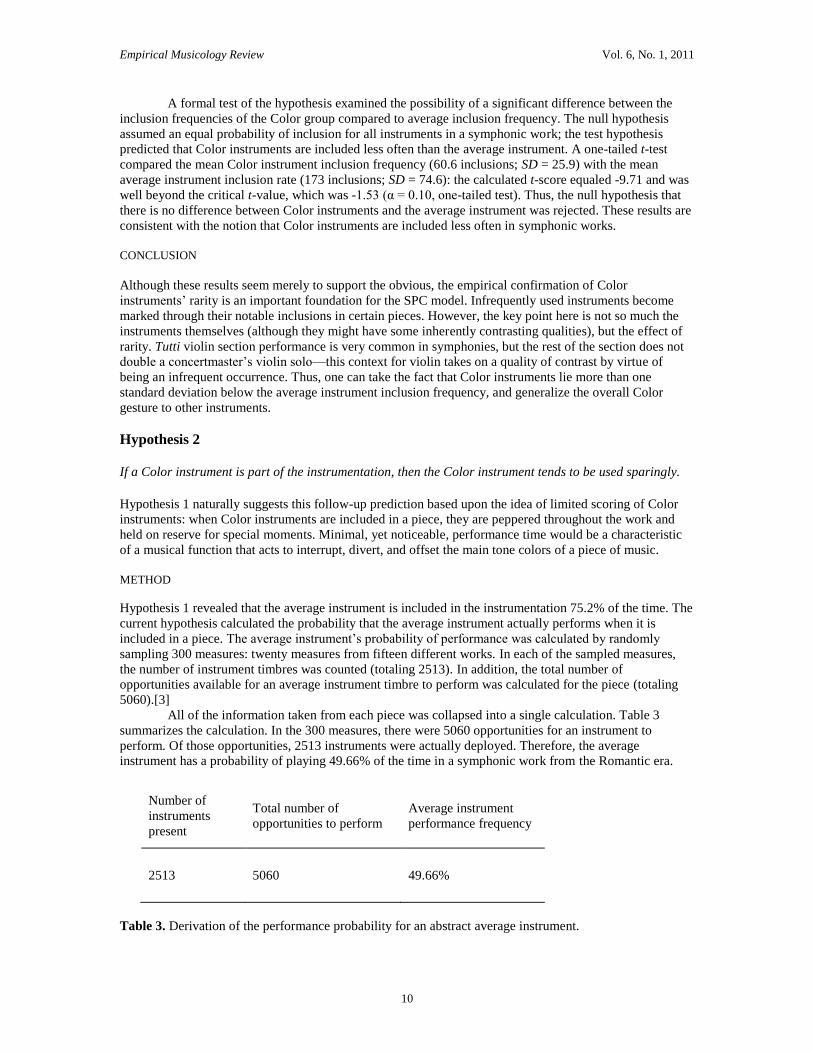
All of the information taken from each piece was collapsed into a single calculation. Table 3
summarizes the calculation. In the 300 measures, there were 5060 opportunities for an instrument to
perform. Of those opportunities, 2513 instruments were actually deployed. Therefore, the average
instrument has a probability of playing 49.66% of the time in a symphonic work from the Romantic era.
Number of
instruments
present
Total number of
opportunities to perform
Average instrument
performance frequency
2513 5060 49.66%
Table 3. Derivation of the performance probability for an abstract average instrument.

Empirical Musicology Review Vol. 6, No. 1, 2011
11
Next, the investigation turned to individual Color instruments. For each instrument, eight pieces
were randomly sampled from the total number of pieces that include the specific Color instrument. Within
each piece, fifteen bars (non-contiguous) were randomly sampled. Then, the presence or absence of the
Color instrument was recorded for each bar. The total number of bars that the Color instrument plays was
then used to calculate a probability that the Color instrument would play in the piece. This process was
repeated for all eight pieces and then the average probability was calculated for each instrument.
RESULTS
Table 4 shows the average performance probabilities for each Color instrument. In addition, the table
shows t-scores for each instrument relative to the average instrument’s inclusion (7.46 performing
moments/15 opportunities).[4] One-tailed t-tests were conducted for all Color instruments (α = 0.10). The
null hypothesis assumed no difference between the frequency of performance of Color instruments and the
average instrument. The hypothesis proposed that Color instruments perform significantly less than the
average. The critical t-score was equal to -1.415.
Instrument Performance frequency average
(out of 15 total opportunities) Percentage Sample size
number of occurrences % n
Bass clarinet 6.63 44.17 8
Contrabassoon 4.88 32.53 8
Cornet 4.75 31.67 8
English horn 4.00 26.67 8
Harp 2.71 18.10 7
Instrument Standard deviation t-Score
SD t
Bass clarinet 2.39 -0.98
Contrabassoon 2.30 -3.17
Cornet 3.54 -2.17
English horn 3.38 -2.90
Harp 3.63 -3.46
Table 4. Performance frequencies and t-scores of Color instruments from samples of eight different works
per instrument.
The one-tailed t-test results show that nearly all of the Color instruments’ performance rates are located
more than two standard deviations away from the mean. The only exception is the bass clarinet. Therefore,
in the case of the harp, English horn, cornet, and contrabassoon, the null hypothesis (that Color instruments
play the same amount as other instruments) was rejected. The results are consistent with the notion that
when Color instruments are included in a work’s instrumentation, they perform significantly less than the
average instrument.
CONCLUSION
Through less performance time, Color instruments would gain an advantage of low listener habituation: if
―auditory fatigue‖ is related to habituation and attention span, then Color instruments could serve to refresh
the orchestral texture and maintain listener engagement with the music. In the case of the bass clarinet, the
null hypothesis failed to be rejected. The mean frequency of bass clarinet performance was not significantly
lower than the mean performance frequency of the average instrument, but it was skewed in the predicted
direction of infrequent use. Taken alone, this result might suggest that the bass clarinet is not a Color
instrument, but a member of another SPC group; alternatively, it could have some Color attributes
combined with some traits from other SPC model groups.
Empirical Musicology Review Vol. 6, No. 1, 2011
12
Hypothesis 3
Non-Color instruments do not solo with the same frequency as Color instruments.
This hypothesis tested one important prediction of Color function: if a Color instrument’s sparing use is
indeed intended to give it an ear-catching contrasting quality, then a Color instrument’s appearance would
align with solo moments in music more so than other instruments. On one hand, composers might prefer to
give solos to Color instruments rather than other instruments because Color instruments’ generally sparing
use lends them an automatic timbral contrast; and their softer tones are best heard in contexts that minimize
masking. On the other hand, solos might be a fairly common occurrence—composers potentially prefer
timbral variety rather than timbral contrast.
METHOD
Defining a ―solo‖ proved to be the most challenging element of this hypothesis test. The spectrum of solo-
like moments includes many types of musical configurations; for example:
A lead voice within a texture of multiple duplications of a melodic line
A unique and melodically prominent, yet accompanied line
An instrument that plays completely alone
The present study hoped to identify solos that are a combination of the second and third bullet
points above, but it was difficult to identify solos using an objective decision process. Due to this difficulty,
solo moments were identified via the expertise of four other musicians who had no knowledge of the
hypothesis currently under investigation. At the time of this study they were graduate students in music
theory, composition, and conducting at Ohio State University. Each musician was given a detailed
instruction sheet that included a definition of a solo: ―One might argue that it is possible to perceive
multiple, simultaneous solo lines, but the present study will exclude this option and consider a true solo as a
line of primary importance that is used in only a single instrument color. The solo will be defined as a line
that does not have to compete with any simultaneous, rival lines. The solo usually has support from lines of
significantly less prominence; sometimes it occurs completely alone.‖ Seventy randomly-selected pages
from the sampled works were given to each musician. Then, the participants used a marker to highlight the
soloing instrument for the complete duration of its solo.
Once the identified solos were collected from the musicians, each highlighted solo passage was
matched with a randomly-selected measure from the same page that contained no solos. This step preserved
the independence of each observed solo, while balancing the moment with a non-solo passage with the
same potential for instrumentation.
The pairing technique defined a ―solo reserve coefficient.‖ This metric is a scale ranging from 0.5
to 1.0—a hypothetical instrument used only for solo moments would have, for example, 10 solo moments
and 0 non-solo moments. The total number of solo measures divided by the total number of measures
performed would be 10/10 = 1.0. The converse situation would be an instrument that played in non-solo
sonorities just as often as it soloed. In this case, there might be 20 solo measure and 20 appearances in non-
solo measures. The ratio of solo measures to the total number of appearances would be 20/40 = 0.5.
Empirical Musicology Review Vol. 6, No. 1, 2011
13
RESULTS
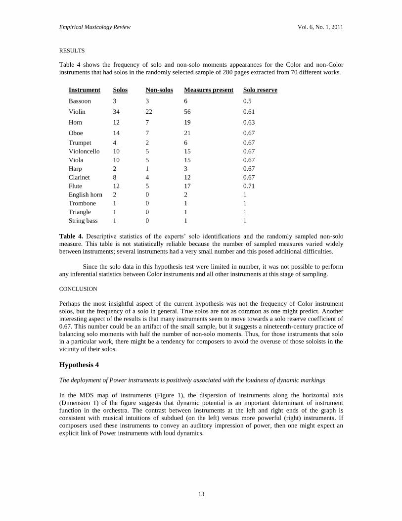
Table 4 shows the frequency of solo and non-solo moments appearances for the Color and non-Color
instruments that had solos in the randomly selected sample of 280 pages extracted from 70 different works.
Instrument Solos Non-solos Measures present Solo reserve
Bassoon 3 3 6 0.5
Violin 34 22 56 0.61
Horn 12 7 19 0.63
Oboe 14 7 21 0.67
Trumpet 4 2 6 0.67
Violoncello 10 5 15 0.67
Viola 10 5 15 0.67
Harp 2 1 3 0.67
Clarinet 8 4 12 0.67
Flute 12 5 17 0.71
English horn 2 0 2 1
Trombone 1 0 1 1
Triangle 1 0 1 1
String bass 1 0 1 1
Table 4. Descriptive statistics of the experts’ solo identifications and the randomly sampled non-solo
measure. This table is not statistically reliable because the number of sampled measures varied widely
between instruments; several instruments had a very small number and this posed additional difficulties.
Since the solo data in this hypothesis test were limited in number, it was not possible to perform
any inferential statistics between Color instruments and all other instruments at this stage of sampling.
CONCLUSION
Perhaps the most insightful aspect of the current hypothesis was not the frequency of Color instrument
solos, but the frequency of a solo in general. True solos are not as common as one might predict. Another
interesting aspect of the results is that many instruments seem to move towards a solo reserve coefficient of
0.67. This number could be an artifact of the small sample, but it suggests a nineteenth-century practice of
balancing solo moments with half the number of non-solo moments. Thus, for those instruments that solo
in a particular work, there might be a tendency for composers to avoid the overuse of those soloists in the
vicinity of their solos.
Hypothesis 4
The deployment of Power instruments is positively associated with the loudness of dynamic markings
In the MDS map of instruments (Figure 1), the dispersion of instruments along the horizontal axis
(Dimension 1) of the figure suggests that dynamic potential is an important determinant of instrument
function in the orchestra. The contrast between instruments at the left and right ends of the graph is
consistent with musical intuitions of subdued (on the left) versus more powerful (right) instruments. If
composers used these instruments to convey an auditory impression of power, then one might expect an
explicit link of Power instruments with loud dynamics.

Empirical Musicology Review Vol. 6, No. 1, 2011
14
METHOD
An ordinal scale was assigned to eight common dynamic markings. The scale shown in Table 5 represents
the loudness hierarchy of dynamic markings and preserves the variance of dynamic markings without
dichotomizing dynamic levels into only two categories, loud and soft.
Dynamic: ppp pp p mp mf f ff fff
Loudness Rank: 1 2 3 4 5 6 7 8
Table 5. Ordinal scale of dynamic strength ratings.
Forty works containing all SPC functional category types were sampled. Within each piece, every
dynamic marking was considered a valid sampling point, but only if there was no dynamic marking
discrepancy between instruments. For example, if the oboe was marked ff and the clarinet was marked mf,
then that point in the music was not included. Each sampling point was a complete measure containing
equal dynamic markings in all instruments. Any marking other than those in the ordinal scale were not used
in the sample.
The dynamic strength and number of Power instruments playing in the sampled measure was
recorded. For example, sampled measure x was selected because there was a consensus between all
instruments on a dynamic marking of mf. This marking was coded as ―5‖ and then the presence of the
trombone, timpani, and trumpet was recorded as ―3‖ Power instruments. Therefore, sampled measure x was
represented by the number pair ―5 – 3.‖
RESULTS
A Spearman rank correlation coefficient established the relationship between the ordinal rank of dynamic
level and the number of Power instruments present in the sampled sonorities. In a total of 1162 measures
the correlation between numbers of Power instruments and dynamic strength was rs = 0.504 (p < 0.01).
This moderate, positive correlation suggests that there is a relationship between dynamic strength and the
number of Power instruments present in a texture. The results are consistent with the hypothesis that the
presence of a Power instrument is associated positively with dynamic loudness levels.
CONCLUSION
Although Power instruments’ order of entry during increases in dynamic strength was not specifically
tested in this hypothesis, it was observed that the horn is nearly ubiquitous at all dynamic levels. During the
score scanning process, it was evident that if only a single Power instrument was present in a texture, then
it was most likely to be the horn. It was usually the first Power instrument added during a large-scale
crescendo and it was commonly the last Power instrument to be removed from the orchestration during a
decrescendo. Nevertheless, the Power group as a whole is associated with louder dynamics.
Hypothesis 5
If Power instruments are present in the musical texture, then the range utilized for the orchestra is wider
than when Power instruments are absent:
Treble instruments will have higher pitch height when Power instruments are used
OR
Bass instruments will have lower average pitch height when Power instruments are used
The results of the previous hypothesis test supported the idea that Power instruments tend to play at louder
dynamic levels. In addition, Power instruments possibly influence the orchestra’s use of pitch extremes. It

Empirical Musicology Review Vol. 6, No. 1, 2011
15
seems counter-intuitive to include the piccolo and tuba into the same functional group; however, the Power
instruments share not only loud dynamics, but also extreme register (both high and low pitch heights).
Although it would be most compelling if Power instruments pushed the pitch range outward in both the
high and low directions, it is possible that Power instruments might expand overall pitch range in one
direction: down or up. Hence, two sub-hypotheses (bulleted under the general hypothesis statement) were
tested to understand the precise direction of pitch range expansion.
METHOD
The initial method, considered for this hypothesis test, planned to 1) sample random sonorities from scores;
2) calculate the pitch height for all performing treble and bass instruments; and 3) average all instruments’
pitch heights together to produce an average treble and bass pitch height for every sonority. While this
approach would have precision, it lacks control over the number of instruments playing in the sampled
sonorities: the sheer number of instruments (regardless of type) could influence the calculated average pitch
range. The following sampling method was used to eliminate the potential confound caused by different
numbers of instruments playing at any given point in time of a symphonic work.
The range fluctuations of two instruments (violin and violoncello) were used as the gauge from
which inferences about the composite range of the orchestra could be made. These instruments were chosen
because of their Standard classification: it was likely that they would perform frequently. The violin
represented the treble range instruments, while the violoncello represented the bass range instruments. If
the addition of Power instruments into the texture has an association with wider pitch range, then one
would expect to see a rise in the violin’s average pitch height, or a falling of the violoncello’s average pitch
height.
The present study collected both of its samples using two different criteria: 1) no Power
instruments present (―non-Power‖ sonorities) and 2) one or more Power instruments present (―Power‖
sonorities). The non-Power sample comprised up to three sonorities randomly sampled from 32 randomly-
selected works (n = 84 sonorities).[5] Each page was scanned from beginning to end, stopping at the first
sonority that contained violin, violoncello, and no Power instrument. If nothing on the page met these
criteria, then successive pages were searched in turn until a non-Power sonority was found. Steps were
taken to prevent accidental re-sampling of any previously sampled sonority. The semitone distances
between each sampled pitch and D4 were averaged together to determine the mean pitch height (Table 6)
for the violin and violoncello in non-Power contexts.[6] The second comparison distribution contained only
sonorities using one or more Power instruments and the violin and violoncello. The sampling technique and
mean pitch-height calculation (Table 6) mirrored the non-Power stage outlined above.
Non-Power Sonorities
Mean (semits) Standard Deviation (semits) n
Violin height 11.50 8.60 84
Violoncello height -10.79 7.58 84
Power
Mean (semits) Standard Deviation (semits) n
Violin height 13.02 9.21 86
Violoncello height -10.52 8.70 86
Table 6. Descriptive statistics for average pitch height, in relation to D4, of violin and violoncello in non-
Power and Power sonorities.

Empirical Musicology Review Vol. 6, No. 1, 2011
16
RESULTS
The hypothesis test used two t-tests (one-tailed) to compare fluctuations of average pitch height in Power
and non-Power sonorities:
The treble range sub-hypothesis predicted that the sonorities containing Power instruments would
have a higher average pitch those without Power instruments. The first t-test compared the range of the
violin between the Power and non-Power samples. The critical t value using an alpha level of 0.10 was tcrit
= 1.292 (df = 80). The calculated t value was t = 1.11, which was smaller than the critical t value—there
was no significant difference of the violin’s average pitch height in non-Power sonorities versus Power
sonorities.
The bass range hypothesis predicted that Power instruments contribute to a downward push of
pitch-height in the orchestra’s bass instruments—represented by the violoncello. Again, the critical t value
was equal to 1.292. The calculated t score for the violoncello was t = 0.210. This also did not meet the
criteria for statistical significance: the presence of Power instruments does not seem to lead to a significant
lowering of violoncello pitch height.
CONCLUSION
Since there was not a statistically significant shift of violoncello or violin pitch height between non-Power
and Power sonorities, there was no support for the overall hypothesis that the presence of Power
instruments is associated with a widening of the average orchestral pitch range. The data collection process
and score study informally reinforced that there is no discernible change of pitch height in Power compared
to non-Power sonorities. Of course, this all rests upon the assumption that the violin and violoncello are
representative of other instruments’ pitch height. A future test of this hypothesis should collect pitch-height
data from all orchestral instruments; it also should make a distinction between the number of Power
instruments present in a texture. The ―one or more‖ sampling criterion was convenient, but could be
imprecise if the number of Power instruments significantly affects pitch range expansion. Power
instruments are indeed dynamically forceful (Hypothesis 4), but they do not seem to function as both power
and range expansion agents.
General Conclusion
Formal tests supported three out of five hypotheses based upon the SPC model; these are mixed results, but
the moderate robustness of the SPC model warrants further investigation. Considering that these five
hypotheses are a subset of a larger number of predictions that could be made by the SPC model, it is
appropriate to reserve judgment about the degree of the model’s accuracy until future studies are
conducted.
Color instruments had a lower likelihood of inclusion and performance in orchestral works—they
are held on reserve. Although they do not appear to have more solos than other instruments, Color
instruments still could stand out from the rest of the orchestra if they have an inherently distinctive timbre,
capable of projecting through, under, or above other groups of instruments.
Power instruments exhibited their namesake characteristic: dynamic strength and numbers of
Power instruments present in the musical texture were moderately correlated. The intuition that Power
instruments also function to expand the range of the orchestra did not gain empirical support. Power
instruments seem to have little effect on the pitch height of other instruments; perhaps Power instruments
themselves are the pitch register ―icing on the cake‖ and solely contribute to a wider orchestral pitch
range—this question was not tested in hypothesis 5 and could be tested in a future study. Hypothesis 5 also
assumed that the violin and violoncello were adequate representatives of the orchestra: this might be false,
so judgment should be suspended until the pitch range test is repeated with more precise measures of the
whole orchestra’s pitch range.
No hypotheses were tested for the Standard instruments. A few predictions were formulated, but
none were deemed important given the restricted scope of the present, exploratory study.

Empirical Musicology Review Vol. 6, No. 1, 2011
17
DISCUSSION
Although the present study puts forward a model of instrument combination in orchestration, this approach
is descriptive and should not be interpreted as a prescription of orchestration patterns. Nor should the study
of orchestration in the Romantic period be construed as a radical effort to reinstate ―ideal‖ principles of
composition. Rather, this approach intends to open up new insights into existing orchestration practices and
possibly to inspire the creation of original, artistic ideas. The terms ―Standard,‖ ―Power,‖ and ―Color‖ were
chosen from several alternatives because SPC best encapsulates some important musical gestures in the
nineteenth-century style of orchestration.
SPC NAME ALTERNATIVES
Examples of alternative names for the SPC groups: 1) Patterns of instruments in groups could be seen to
reflect a historical progression of instrument use in symphonic music. One might use terms like ―Old‖,
―Newer‖, and ―Newest‖ (ONN)—these adjectives refer mainly to the time of instruments’ adoption into the
orchestra and not their absolute age. The Standard instruments (plus the trumpet, horn, and timpani)
comprise the complete orchestra used in the Classical period. The Power group contains instruments like
the trombone, which existed long before the nineteenth century (i.e., the sackbut), but were newer additions
to the symphonic genre and gained more freedom of expression via major technological advances in the
Romantic period (e.g., valves for trumpets and horns). The Color group has instruments that either did not
exist until the nineteenth century (e.g., the cornet) or were significantly improved in the nineteenth century
to warrant their use in the orchestra. The ONN group names were not used because they only loosely reflect
instrument timelines; plus, it is unlikely that composers would distribute instruments solely based upon
their ―age‖ in the orchestra. 2) Alternatively, SPC groups might be called ―Most Frequent,‖ ―Less
Frequent,‖ and ―Least Frequent‖ (MLL) in reference to instrumentation frequency; Figure 3 suggests this
stratification—with exception to the horn—but the MLL explanation is weaker than the SPC model. MLL
does not suggest a goal-oriented element in instrument use—for example, that Power instruments are well
suited to loud dynamics or that Color instruments are lower or warmer variants of other instruments.
LIMITATIONS AND PROMISES OF THE SPC MODEL
By no means does the SPC motto preclude other large-scale functions or confine instruments into a single
category; rather, the SPC model suggests that composers sometimes combine entire instrument families
(Standard = Woodwinds + Strings), or combine instruments between instrument families. The resulting
combinations look to be aligned with three purposes: 1) Establish a tone-color foundation and reference
point (Standard); 2) Provide loud dynamic contrasts and climaxes (Power); and 3) Create timbral contrast
using rarer, lower, or more mellow instruments (Color). It would be very exciting to see other functions
emerge from further study of both the nineteenth century and other time periods; an important place to start
is with percussion instruments, which were excluded from the SPC model.
The present study used only snapshots in time as representatives for orchestration patterns—
patterns that are, in reality, continuously in flux during performances of symphonic works. Future studies
could look at temporal variables such as instrument entrances and exits from the texture during crescendi
and decrescendi, for example. Additionally, it would be important to show that orchestral gestures are
primary and the instruments in those groups are secondary: if this is true, then one might expect to see a
stable repertoire of gestures, but with instruments that can assume alternative roles as they dissolve away
from one group and join another group. Instrument fluidity in conjunction with gestural stability seems to
be one characteristic of twentieth-century orchestration, which combines instruments quite flexibly and
imaginatively; instrument combinations appear to fulfill a number of roles depending upon the use of
extended techniques (e.g., multiphonics; altissimo effects; key slaps) or the use of mutes.
The SPC model has broad applications for the development of new musical analysis techniques
and also for the continued construction of orchestration theory; there are fruitful insights that lie ahead.
Despite orchestration’s vast importance, it has eluded many musical analysis techniques. As a consequence,
music-theoretic approaches generally have not treated concerns of orchestration in as great of depth as
other primary musical parameters (e.g., harmony, melody). This is not surprising considering western art
music’s notation, which explicitly specifies pitch and rhythm, but imprecisely represents other vital sound
characteristics like tone quality and balance (Palmer, 1997). Orchestration treatises largely discuss the first-

Empirical Musicology Review Vol. 6, No. 1, 2011
18
order properties of individual instruments, but these issues are more appropriately thought of as
―instrumentation‖ issues. Orchestration involves the higher-order processes of instrument combination,
instrument orderings, pitch distribution among instruments, and many other elements—ones that could lead
to bountiful musical discoveries if future studies examine them in detail. The SPC theory not only describes
the impetus of gesture on instrument combination, but the method also shows how a hybrid artistic-
empirical approach can take the multi-faceted contributions from diverse fields of inquiry and bridge them
with orchestration theory.
NOTES
[1] Typical chapter subheadings are organized around instrument families. For example: ―Scoring for
Strings‖ and ―Scoring for Woodwinds,‖ see Blatter (1997) and other orchestration texts (Piston, 1955;
Rimsky-Korsakov, 1964[1913]). While headings concerning combinations across instrument families do
occur, the treatment of this topic is minimal when compared to the treatment of scoring within families.
[2] The Proxcal 1.0 algorithm by the Data Theory Scaling System Group (DTSS) of the Faculty of Social
and Behavioral Sciences, Leiden University, The Netherlands, was used for this analysis. The present study
used 10 random starts for the initial configuration of the instruments; interval transformation was used for
the dissimilarity measures.
[3] Percussion instruments were included in this calculation. The percussion section might operate as a
single entity in some cases, but at the same time, the section is composed of many different timbres. The
calculation considered each different percussion instrument as a separate timbre opportunity.
[4] The value of 7.46 came from the average instrument’s performance frequency (49.66%) relative to 15
performance opportunities.
[5] The non-Power sonority sample was slightly smaller than the expected n = 96 because it was overly
time-consuming to search for non-Power sonorities that had a nearly constant presence of one or more
Power instruments: sometimes pieces appeared to have less than three instances of a non-Power sonority.
These examples were usually shorter symphonic pieces, but this observation is nevertheless a challenge to
the notion that Power instruments provide contrast to the prevailing orchestration – Power instruments are
sometimes quite prevalent.
[6] D4 represents the average notated pitch of western classical music; see Huron (2001).
REFERENCES
Blatter, A. (1997). Instrumentation and Orchestration (2nd ed.). New York: Schirmer Books.
Caclin, A., McAdams, S., Smith, B.K., & Winsberg, S. (2005). Acoustic correlates of timbre space
dimensions: A confirmatory study using synthetic tones. Journal of the Acoustic Society of America, Vol.
118, No. 1, pp. 471-482.
Daniels, D. (2005). Orchestral Music: A Handbook (4th ed.). Lanham, MD: Scarecrow Press.
Dubal, D. (2001). The Essential Canon of Classical Music. New York: North Point Press.
Grey, J. (1977). Multidimensional perceptual scaling of musical timbres. Journal of the Acoustical Society
of America, Vol. 61, No. 5, pp. 1270-1277.
Huron, D. (2001). Tone and voice: A derivation of the rules of voice-leading from perceptual principles.
Music Perception, Vol. 19, No. 1, pp. 1-64.
Empirical Musicology Review Vol. 6, No. 1, 2011
19
McAdams, S., Winsberg, S., Donnadieu, S., De Soete, G., & Krimphoff, J. (1995). Perceptual scaling of
synthesized musical timbres: Common dimensions, specification and latent subject classes. Psychological
Research, Vol. 58, pp. 177-192.
Palmer, C. (1997). Music performance. Annual Review of Psychology, Vol. 48, pp. 115-138.
Piston, W. (1955). Orchestration. New York: Norton.
Rimsky-Korsakov, N. (1964). Principles of Orchestration (M. Steinberg, Ed. & E. Agate, Trans.). New
York: Dover. (Original work published 1913).
Sandell, G.J. (1991). Concurrent Timbres in Orchestration: A Perceptual Study of Factors Determining
“Blend”. Ph.D. dissertation. Northwestern University.
Top Related