


Languages
Pages
Legal


1
The Real Impact of Improved Access to Finance:
Evidence from Mexico
MIRIAM BRUHN AND INESSA LOVE *
Article forthcoming in The Journal of Finance
ABSTRACT
This paper provides new evidence on the impact of access to finance on poverty. It
points out an important channel through which access affects poverty – the labor
market. The paper exploits the opening of Banco Azteca in Mexico, a unique
“natural experiment” in which over 800 bank branches opened almost
simultaneously in pre-existing locations of Elektra stores. Importantly, the bank has
focused on previously underserved low-income clients. Our key finding is the
sizeable effect of access to finance on labor market activity and income levels,
especially among low income individuals and those located in areas with lower pre-
existing bank penetration.
Keywords: Finance and Development; Entrepreneurship; Banking.
JEL codes: G12, O12
* Miriam Bruhn is at the World Bank, Inessa Love is at the University of Hawaii at Manoa and the World Bank. We
thank the Knowledge for Change Program for supporting this project with funding and Kiyomi Cadena for
providing excellent research assistance. We are also grateful to David McKenzie and to James Vickery for their very
useful comments. The views expressed in this paper do not necessarily represent those of the World Bank, its
Executive Directors, or the countries they represent. Corresponding author: Miriam Bruhn, The World Bank, MSN
MC 3-307, 1818 H Street, NW, Washington, DC 20433, USA. Phone: 202-458-2732, Fax: 202-522-1155,

2
It has been well recognized that financial development is important for economic growth
(Levine, 2005). In addition, several recent papers have found a positive correlation between
access to finance and poverty alleviation at the country level (Beck, Demirguc-Kunt and Levine,
2007, Honohan, 2004, and World Bank, 2008). However, these papers tend to face identification
issues, implying that they do not necessarily establish a causal relationship between access to
finance and economic outcomes. Similarly, while the microfinance industry has grown
exponentially in the past few decades and many researchers have written on the topic,1 there is
still little systematic evidence on the casual impact of microfinance on economic activity
(Harford, 2008, and Karlan and Morduch, 2009). This paper seeks to fill this gap and to add new
evidence on the impact of access to finance on poverty.
Such evidence is especially important given that several recent randomized evaluations
have questioned the large role previously attributed to microfinance in poverty alleviation.2
These studies have intensified the debate on the role of finance in reducing poverty and have
highlighted the importance of measuring plausible magnitudes of the effect. This paper adds to
the debate by providing estimates that suggest that improving access to finance for low income
individuals can play an important role in poverty alleviation.
In addition, there is little evidence on the channels through which finance may help to
reduce poverty. This paper offers evidence on one such channel: the labor market channel. The
role of finance in the labor market has come to be seriously questioned after the recent financial
crisis, which resulted in enormous job losses, particularly in countries with more developed
financial sectors (Pagano and Picca, 2012). In contrast, we find that there is a significant and

3
positive impact of financial access on labor market outcomes. These results suggest that finance
may alleviate poverty, at least partially, through its labor market effects.
Finally, this paper provides new insights that may influence the effectiveness of
microfinance institutions (MFIs). We study the impact of a new bank for low income individuals,
that has been able to leverage its relationship with a large retail chain to reduce transaction costs,
acquire effective information, and enforce loan repayment. We discuss how these features can
solve several problems that constrain standard MFIs and allow them to play a larger role in
poverty alleviation. The paper offers concrete suggestions on how policymakers can spur access
to finance.
Specifically, we use a unique event – the opening of Banco Azteca in Mexico in October
2002 – to evaluate the effect of increased access to financial services for low-income individuals
on entrepreneurial activity, employment, and income. This event was unique in that Banco
Azteca opened branches in all of the existing stores of its parent company – a large retailer of
consumer goods, Grupo Elektra. Almost overnight, Banco Azteca established the second largest
network of branches in the country. This set a world record of a bank opening more than 800
branches at once.
An important feature of Banco Azteca was that from the start it catered to low and
middle-income groups which had mostly been excluded from the commercial banking sector3.
Capitalizing on Grupo Elektra’s decades of experience in making small installment loans for its
merchandize, rich data, and established information and collection technology, the bank was
uniquely positioned to target this segment of the population, which it estimated to comprise over

4
70% of all households. Many of these households were part of the informal economy – operating
small informal businesses that lacked the documentation necessary for obtaining bank loans. The
nature of Azteca’s operations, including low documentation requirements and the motorcycle-
riding loan officers that come to the borrower’s house, as well as the size of the loans offered
make it comparable to MFIs that operated in Mexico at the time of Azteca opening. However,
there are also important differences with MFIs that we discuss later.
We use the predetermined nature of the branch locations – which were opened in all
stores of its parent company, Grupo Elektra – to identify the casual impact of Azteca opening on
economic activity through a difference-in-difference strategy. Specifically, we compare the
changes in outcome variables before and after Azteca opening across municipalities with pre-
existing Grupo Elektra stores and those without stores at the time of the bank opening. Our
analysis controls for the possibility that time trends in outcome variables may be different in
municipalities that had Grupo Elektra stores and those that did not. Using the Mexican Labor
Market Survey, ENE, we study the impact of this event on individuals’ employment choices and
income levels.
We have five main findings. First, the new bank opening led to an increase in the
proportion of informal businesses by 7.6%%, but to no change in formal businesses. This is
consistent with anecdotal evidence suggesting that Azteca targeted lower-income individuals and
also with Azteca’s low documentation requirements. In contrast, formal business owners have
easier access to commercial bank credit, and likely prefer it because of higher interest rates
charged by Azteca4.

5
Second, the new bank opening led to an increase in income levels by about 7% on
average over two years. Similarly to this result, Burgess and Pande (2005) find that the
expansion of bank branches in rural India had a significant impact on alleviating poverty,
although Kochar (2005) and Panagariya (2006) cast doubt on their findings.
While Burgess and Pande do not examine the channel through which increased bank
presence alleviates poverty, we are able to investigate the effect of Banco Azteca opening in
more detail, by considering how the impact varies with pre-event occupation. We find that the
increased availability of financial services helped existing informal business owners to continue
their operations instead of closing their business and transitioning to being the wage-earners or
not employed. This is consistent with evidence suggesting that micro entrepreneurs have very
high rates of return on capital, and hence would benefit from increased access to finance (See
McKenzie and Woodruff, 2008, and De Mel, McKenzie, and Woodruff, 2008)5.
Third, Banco Azteca opening led to a reduction in the proportion of not employed
individuals by about 1.4% and increased income for this segment of the population.6 This is
because some previously not employed individuals opened informal business and others were
more likely to work as wage earners after Banco Azteca opening. These results on employment
and income mirror’s Karlan and Zinman (2010) finding that increased availability of consumer
credit has a range of positive outcomes on the household well-being, including an increased
ability to retain employment and increased income. Karlan and Zinman’s analysis includes only
individuals that work as wage earners. Our study, however, shows that increased access to
finance has positive effects on self-employment, as well as on wage work.

6
Fourth, we find that the impact was heterogeneous across different segments of the
population by performing two sample splits. First, consistent with the fact that Azteca targeted
the low to middle income population, we find that its impact was larger for individuals with
below median income levels. Second, we find that the impact was larger in municipalities that
were relatively underserved by the formal banking sector before Azteca opened (measured by
demographic bank branch penetration). These results confirm that the channel through which
Banco Azteca had an impact on real activity was operating through an increased access to
financial services.
Finally, we show that real GDP per capita growth rates have also increased following the
introduction of Banco Azteca. These growth results further illustrate the positive effect that
access to finance for low income individuals has on economic activity and on income.
Our paper is related to a literature on US banking deregulation, which exploits the natural
experiment of gradual relaxation of restrictions on state-wide branching and on entrance by out
of state banks. This relaxation of restrictions resulted in increased presence of banks in different
states, which is somewhat akin to the entry of Banco Azteca. Some of the results of this literature
parallel ours: Jayarathne and Strahan (1996) find an increase in the economic growth rate by
0.51-1.19%. Black and Strahan (2002) find an increase in new firm incorporations by up to 8%.
Also closely related to our work, Beck, Levine and Levkov (2007) find that banking
deregulation resulted in a reduction in income inequality through the impact on labor market
conditions. While we do not test for this directly in this paper, the entrance of Banzo Azteca has
likely led to increased bank competition, similar to what Cetorelli and Strahan (2006) find in the

7
US: they argue that deregulation has led to increased competition and a larger presence of small
firms. Despite some similarities with previous research, the unique feature of Banco Azteca,
namely the targeting of low income, previously unbanked individuals, make it an important case
for studying the real effects of bank expansion.
The rest of the paper is organized as follows. Section I offers a detailed background on
Banco Azteca opening and its impact on the financial sector, as well as a comparison between
Azteca and MFIs. Section II lays out our empirical strategy. Section III describes the data.
Section IV presents our regression results, and Section V concludes.
I. Background on Banco Azteca
I.A. Characteristics of Banco Azteca
In March 2002, one of Mexico’s largest retailers for electronics and household goods,
Grupo Elektra, received a banking license. In October 2002, Grupo Elektra launched Banco
Azteca, opening a total of 815 branches in all pre-existing Grupo Elektra stores. From the outset,
Banco Azteca targeted low and middle income customers, historically underserved by the
traditional banking industry. As the New York Times reports: “The bank was the first and only
all-Mexican-owned franchise to be licensed by the Finance Ministry since 1994. It is also the
first bank to aim at Mexico's middle and working classes: the 73 million people who live in
households with combined family incomes of $250 to $4,000 a month, a mass market largely
neglected by Mexico's banking system.”7

8
Banco Azteca benefited from synergies with their retail operations, which provided a rich
source of data on their customers. With Elektra's 48 years of know-how in selling goods on
installment to lower-income consumers, Banco Azteca had information on about 4 million
borrowers. Many of these borrowers buy Elektra's products, develop film at its stores or receive
money transfers from the United States through Western Union. “We know this segment of
Mexican society better than anyone else,” says Banco Azteca President Carlos Septien.8 “The
sophisticated technology and collection systems already in place at Grupo Elektra will provide us
with invaluable data about our customers’ buying habits and financial needs, allowing us to
succeed.” The fact that Azteca branches are located in Elektra stores where clients make other
purchases and transactions also has marketing benefits since it brings the bank closer to
individuals who may otherwise be reluctant to approach a traditional commercial bank for a loan.
The bank also inherited a 3,000-strong army of motorcycle-riding loan agents. These
agents carry handheld computers loaded with Elektra's rich database, which includes customers’
credit histories and even names of neighbors who might help track down delinquent debtors.9
“The difference between Elektra and more established banks is that Elektra has a much better
collection system,” said Joaquin Lopez-Doriga, an analyst with Deutsche-Ixe. “If you want to
address the market that Elektra is addressing, you have to know it very well. That's very labor
intensive.” 10
Azteca also requires less documentation than traditional commercial banks, often taking
collateral and co-signers instead of valid documents. For example, Business Week11
reported an
account of an informal carpenter with no proof of income obtaining an Azteca loan using as

9
collateral the items he bought on credit from Elektra stores in the past three years. Despite the
high interest rate (48% per annum), the carpenter reported: “I don’t really have any other
options.” Even today, many of Azteca customers are informal business owners who do not have
the proof of income required by other banks.
In summary, its unique information and collection technology and synergies with Elektra’s
retail operations have allowed Banco Azteca to extend credit to segments of the low-income
population that were previously un-bankable.
I.B. Increase in Availability of Financial Services
Azteca began its operations by offering savings accounts targeted to low-income customers
that could be opened with as little as $5. Within the first month, 157,000 accounts were opened,
increasing to 250,000 accounts by the end of December 2002. At its opening in October 2002,
Banco Azteca also took over the issuance of installment loans, which were previously issued by
Elektrafin, the financing unit of Grupo Elektra’s retail stores. These loans had an average amount
of $250. Although these loans were tied to merchandize, they could be used for business
purposes. For example, purchasing a new sewing machine or a fridge might allow a person to
start or to sustain their micro business. In 2003, Azteca started offering $500 consumer loans not
tied to the merchandize, with an average term of one year (Grupo Elektra’s 2003 and 2004
Annual Reports). Towards the end of 2003, Azteca also expanded into the mortgage and
insurance business.

10
Although Grupo Elektra was disbursing installment loans before opening Banco Azteca,
Banco Azteca’s new savings accounts allowed its loan portfolio to expand significantly. Figure 1
plots Grupo Elektra’s loan portfolio within Mexico over time, showing a steep increase from the
fourth quarter of 2002 on. The loan portfolio increased from around 2 billion Mexican pesos at
the time of opening Banco Azteca to 10 billion Mexican pesos in the last quarter of 2004.
Although this portfolio size is small compared to the total commercial bank credit to the private
sector, which was about 550 billion Mexican pesos in the fourth quarter of 2002, it is large
compared to the credit disbursed by smaller institutions which cater to low-income households.
The combined portfolio of the largest microfinance institutions in Mexico stood at only 0.5
billion Mexican pesos in the fourth quarter of 2004. In this same quarter, the total amount of
outstanding loans from credit unions was 8.7 billion Mexican pesos.
Figure 2 shows the relative difference in the number of savings accounts in municipalities
with Azteca, vs. municipalities without Azteca. Data on savings accounts comes from the
Mexican bank supervisory body, the Comisión Nacional Bancaria y de Valores (CNBV). There
is a clear rapid growth in savings accounts in municipalities with Azteca after December 200212
.
These effects are also significant in a regression framework that controls for municipality-
specific time trends.
In a related paper Ruiz (2011) shows that individuals in municipalities where Banco Azteca
opened were three times more likely to use bank credit and 46% less likely to obtain pawn-shop
credit. Thus, the opening of Banco Azteca had a non-trivial impact on availability of financial
services in municipalities where the branches were present.
Figure 1
about here
Figure 2
about here
11
I.C. Comparison of Azteca and Microfinance Institutions
Banco Azteca was similar to microfinance organizations (MFIs) in several respects. First,
as noted above, Azteca offered loans of $250-$500. This is comparable in size to loans offered
by several microfinance organizations, which in 2002 amounted to about $360.13
The second
similarity lies in the type of client served by Azteca and MFIs. As discussed above, Azteca had
low documentation requirements and hence was able to extend loans to informal businesses.
Furthermore, it explicitly targeted low income segments of the population, similar to MFIs.
However, there are several important differences between Azteca and MFIs. First, Azteca
was able to accept deposits, which reduced its cost of funds and enhanced its growth
opportunities, while MFIs are usually funded by donor funds or other capital. Second, Banco
Azteca was regulated and supervised as any other commercial bank and hence it had to comply
with CNBV reporting requirements and has participated in the deposit insurance program. In
contrast, MFIs are not regulated as banks, they cannot take deposits and they are not required to
comply with reporting requirements. As a result, accounting information reported by MFIs is
often deemed less reliable than that of regulated banks. In particular, MFIs usually underestimate
non-performing loans (NPL’s) and are more lenient with restructuring loan terms. Third, Azteca
was uniquely positioned to take advantage of economies of scale due to the synergies with its
parent company, Grupo Elektra. As a result, it had a significant advantage in information
technology and collection mechanisms. These differences allowed Azteca to reduce operating
costs despite the small loan size.

12
We present a comparison of Azteca and MFI operating costs, interest rates and default rates
in a Table AI of the Internet Appendix. The data on Azteca come from the CNBV and the data
on MFIs come from MIXmarket.org. Because Compartamos was unique among Mexican MFIs
in many respects (such as going public with a controversial initial public offering in 2007, as
discussed in Cull et al. 2009), we present data separately for Compartamos and the rest of
Mexican MFIs.14
Operating costs are measured as non-interest expenses over assets, the interest
rate is given by the ratio of interest income and fee income on loans to total loans, and the NPL
is the ratio of problem loans to total loans, which is a commonly used measure of the default rate.
The interest rate captures the average effective interest rate on loans.
Table AI of the Internet Appendix shows that Azteca has lower operating costs than MFIs.
Compartamos has lower operating costs than the average MFI, but higher costs than Azteca.
With respect to interest rates, Azteca was able to charge lower rates than MFIs. On average, the
rates were about 40% for Azteca, in the 70% to 90% range for Compartamos, which is well
known for its high interest rates, and about 60% to 70% for other MFIs. Again, Azteca’s lower
operating costs were likely a factor that allowed it to charge lower interest rates than MFIs.
Finally, in terms of default rates, Azteca has lower default rates than reported by most MFIs, but
higher than those of Compartamos.15
To summarize, these comparisons confirm the assertions made above that Azteca’s
information and collection technology and synergies with Elektra’s retail business have indeed
contributed to its lower operating costs and have allowed it to charge lower interest rates. The
Azteca model may offer several solutions to the drawbacks of standard MFIs, specifically the

13
methods to reduce operating costs. In the conclusion (Section V), we discuss the policy
implications derived from Banco Azteca’s features and experience and suggest specific measures
that can spur access to finance for low income individuals.
II. Identification Strategy
In order to identify the effect of Banco Azteca opening on economic activity, we exploit
the cross-municipality and cross-time variation in Azteca branches. As discussed above, Banco
Azteca opened in October 2002, only in the municipalities that had pre-exiting Grupo Elektra
stores. This allows us to estimate the following difference-in-difference regression, which
compares municipalities with and without Banco Azteca before and after Azteca opening:
ictictcttcict ZAztecay ** ,
where i denotes individuals, c denotes municipalities, and t denotes quarters. ß is a set of
municipality fixed effects, γ is a set of quarter fixed effects and Z is a matrix of individual
control variables and y is one of our outcome variables, such as an indicator for employment
status (formal or informal business owner, wage earner or not employed) or income level
(described in more details in the next section). Our main variable of interest is the Azteca
dummy, which is the interaction between a post third quarter of 2002 dummy and a dummy that
equals one for municipalities that had at least one Azteca branch in the fourth quarter of 2002
and that equals zero for all other municipalities in our sample. The coefficient δ is our estimate
of the effect of Banco Azteca opening. We cluster standard errors at the municipality level.16
14
The assumption needed to guarantee that this identification strategy is valid is that, in the
absence of Banco Azteca opening, the average difference between outcome variables across
municipalities with and without Azteca would have been the same post-October 2002 as pre-
October 2002. That is, outcome variables can differ in levels across municipalities with and
without Azteca, but they cannot differ in changes.
This assumption would be violated if, for example, the number of informal businesses
were on a steeper growth path in municipalities with Azteca than in municipalities without
Azteca. If this were the case, we could detect a positive effect of Banco Azteca opening on the
number of informal businesses, when there was actually no effect.
While the identification assumption is fundamentally untestable since we do not observe
the counterfactual of Banco Azteca not having opened, we verify whether the assumption is
likely to hold in three different ways. First, as is common in the literature, we test for parallel
pre-event trends in outcome variables across municipalities with and without Azteca. If the
changes were the same in the pre-period, they are likely to have remained the same in the post-
period in the absence of Azteca opening.
Second, we run regressions that control for the possibility of municipalities with and
without Azteca having different linear time trends. If our estimated effects are driven entirely by
differences in trends, then these effects should disappear once we control for time trends in the
regressions. We do this in three ways: First, we allow all municipalities with Azteca branch to
have the same time trend, and all municipalities without Azteca branch to have a different time
trend. Second, we allow each municipality to have its own time-trend (i.e. municipality-specific

15
time-trends). Third, we investigate the selection process for Elektra and include additional
municipality characteristics interacted with time trends to account for the possibility that such
characteristics might be driving our results.
Finally, we examine graphically whether the estimated change in outcome variables in
municipalities with Banco Azteca coincides with the time of Banco Azteca opening.
III. Data
All of our main outcome variables come from the Mexican National Employment Survey
(ENE). The ENE is the survey that the Mexican government relies on for calculating
unemployment statistics and for measuring the size of the informal sector. It has been conducted
quarterly since 2000-II and covers a random sample of approximately 150,000 households each
quarter. Households remain in the survey for five consecutive quarters. We use data for 2000-II
to 2004-IV (19 quarters in total). After 2004-IV, the ENE was changed to a new survey17
.
We chose to use the ENE data in our analysis for the following reasons. First, it includes
detailed questions about a person's economic activity (including self-employment), and it also
reports a person’s income from their main occupation. Second, it captures and distinguishes
between formal and informal self-employment and firms, making it possible to investigate the
effect of Banco Azteca on informal firms. This is important since many of the Banco Azteca
clients are likely to be informal business owners, as discussed above. Third, the ENE covers a
wide range of municipalities for ten quarters before Banco Azteca opened and nine quarters
after, allowing us to implement the identification strategy described above18
. Fourth, the panel
16
structure of the ENE allows us to describe the effect of Banco Azteca more precisely by looking
at the impact on different pre-reform occupation groups.
The ENE covers a total of 1,222 municipalities, but we drop the ones that do not have
any bank (i.e. neither an Azteca branch, nor any other bank branch) since Azteca opened almost
exclusively in municipalities that already had a branch of a different bank.19
We determine which
municipalities had a bank branch in the fourth quarter of 2002 and which had an Azteca branch
by referring to data from the Mexican bank supervisory body, the Comisión Nacional Bancaria y
de Valores (CNBV). Our final sample includes 576 municipalities, of which 249 had an Azteca
branch in fourth quarter of 2002, and 327 did not have an Azteca branch, but had a branch of a
different bank. Figure 3 shows a map of Mexico where municipalities that had an Azteca branch
in the fourth quarter of 2002 are marked in dark blue, and municipalities that had a different bank
branch, but no Azteca branch, are marked in light blue. Both types of municipalities are
distributed throughout Mexico.
Since our analysis applies to potential Banco Azteca clients who could be economically
active, we keep only individuals of working age (between the ages of 20 and 65) in our sample.
We then construct three of our main outcome variables by creating dummy variables for each
person in the sample, indicating whether the person a) owns an informal business, b) owns a
formal business, and c) is a wage earner.20
These are the three possible occupations for
somebody who is employed. People who do not fall into either of these categories are not
employed (they are either unemployed or not in the labor force).
Figure 3
about here

17
All dummies are defined for the whole sample, meaning that they denote the percentage
of all individuals in the sample who fall into each category. For example, a value of 0.08 of the
formal business owner dummy means that 8% of all people between the ages of 20 and 65 own a
formal business.
Finally, we also use monthly income as an outcome variable. While the dummy variables
are defined for everybody in our sample, income is available only for the gainfully employed and
is missing for the unemployed, for individuals who are out of the labor force, and for unpaid
workers. Unfortunately, the income data from the ENE is probably not as reliable as the
occupation data since it is not the focus of the survey. The survey only includes one question on
income, asking for the earnings from the individual’s main occupation. 4.2% of employed
individuals do not answer this question. These individuals are then asked to report their income
in terms of bins of the minimum wage. About 60% of the people who did not report their income
in the first question report it in terms of the minimum wage (2.4% of the total sample). Taking
these responses into account, we create a dummy variable indicating whether an individual earns
above minimum wage21
. We use this as an additional outcome variable.
The upper panel of Table I, Panel A, includes summary statistics for the outcome
variables split up by municipalities that had at least one Azteca branch in the fourth quarter of
2002 and by municipalities that didn’t have any Azteca branch at that time, but that had at least
one branch from a different bank. The data in Table I are for the pre-Banco Azteca period,
including only observations between 2000-II and 2002-III. The averages in Columns 1 and 2 of
Table I show that, in municipalities with Azteca, 8.2% of people in the sample owned an
Table I
about here

18
informal business in the pre-Azteca period. This number was higher for municipalities without
Azteca, 13.8%. There is a somewhat smaller percentage of formal business owners, 7.9 in
municipalities with Azteca and 6.6 in other municipalities. Another 50% (44%) of our sample
worked as wage earners in municipalities with (without) Azteca. The remaining 34% (36%) of
the sample were not employed.
The third column of Table I, Panel A, reports the differences in pre-reform averages for
municipalities with and without Azteca and their statistical significance. Individuals who live in
municipalities with Azteca are more likely to be employed, more likely to work as wage earners,
and more likely to own a registered business. However, they are less likely to own an informal
business. Moreover, individuals in municipalities with Azteca have a higher average monthly
income than individuals in municipalities without Azteca.
The fact that pre-Azteca outcomes were different across our group of treatment and
control municipalities does not per se invalidate the identification strategy, but differences in
levels may be correlated with differences in changes. As discussed in Section II, the
identification strategy assumes that changes in outcome variables (not levels) are the same in
municipalities with and without Azteca. The lower part of Table I, Panel A, compares pre-period
changes in outcome variables across Azteca and non-Azteca municipalities. There was no
statistically significant difference in average changes across these municipalities for the informal
and formal business owner dummies. The fraction of wage earners, however, decreased in
Azteca municipalities in the pre-Azteca period, while it increased in non-Azteca municipalities.
This is also reflected in the fact that the fraction of people who are not employed increased in
19
Azteca municipalities while it decreased in non-Azteca municipalities. These differences in
changes are statistically significant and would bias our results against finding a positive effect on
the fraction of wage earners. Similarly, the fraction of people who earn above minimum wage
and also log income increased more in non-Azteca municipalities than in Azteca municipalities,
which could also bias our results against finding a positive effect on these income variables. In
our regressions, we control for different linear time trends in Azteca and non-Azteca
municipalities to correct for these biases. Overall, there is no indication that differences in trends
across municipalities could lead us to find a positive effect that is not actually there, implying
that our estimates are on the conservative side.
To further investigate pre-Azteca differences across municipalities, in Table I, Panel B,
we report GDP per capita levels and growth rates for Azteca and non-Azteca municipalities. This
data comes from the 1994 and 1999 Economic Census, as well as the 1995 and 2000 Population
Censuses (municipal level GDP is only available every five years). The table shows that Azteca
municipalities had higher average GDP per capita than non-Azteca municipalities in 1993 and
1998. However, non-Azteca municipalities had a higher average GDP per capita growth rate
from 1993 to 1998. This pattern suggests that income was converging across Azteca and non-
Azteca municipalities in the pre-Azteca period22
and it is consistent with what we reported in
Panel A using labor market survey (ENE) data. The lower growth rates in Azteca municipalities
prior to Azteca opening may bias our analysis against finding a positive impact of Azteca
opening. Thus, it is important to control for pre-existing trends in our regressions, which is our
preferred specification.

20
We also use a number of individual background variables from the ENE as control
variables in the regressions. These variables include age, gender, marital status, and education
dummies. Summary statistics for these background variables and their pre-period changes are in
Internet Appendix Table AIII.
IV. Results
IV. A. Business Owners
We first investigate the impact of Banco Azteca opening on entrepreneurial activity. Table
II presents the results for the informal and formal business owner dummies as dependent
variables. We find that the opening of Banco Azteca had a positive and statistically significant
impact on the fraction of informal business owners. The coefficient on our variable of interest
remains statistically significant and similar in size when we include a separate time trend for the
group of Azteca and non-Azteca municipalities in the regressions (Column 2). The coefficient is
also similar when including municipality specific time trends (Column 3). Overall, the results
suggest that the opening of Banco Azteca increased the fraction of informal business owners by
0.0062, which corresponds to 7.6% of the pre-Azteca fraction of 0.082.
The effect on registered business owners is negative in the specification without time
trends, but this effect is not robust to including time trends in the regression. It is perhaps not
surprising that the fraction of formal business owners did not increase due to Banco Azteca
opening. In contrast to informal business owners, formal business owners typically have access
to commercial banks, since they have the necessary documentation, and commercial banks tend
Table II
about here

21
to offer lower interest rates. While not statistically significant in our preferred specifications, the
negative result for formal business owners could be due to increased competition from informal
businesses. It is also plausible that increased access to finance for informal businesses may
reduce incentives for business formalization, particularly since gaining access to finance is one
of the reasons why businesses become formal. This may not be socially desirable because of a
reduction in the tax base and lowered opportunities for growth and expansion of the business.
Policymakers may reduce any potentially negative impact on formal firms by making it easier
and less expensive to register formal businesses and by reducing the tax burden on formal
businesses.
Figure 4 is a graphic illustration of the effect of Banco Azteca opening on informal
business owners. It displays the fraction of informal business owners in municipalities with and
without an Azteca branch in 2002-IV over time. We observe a steep increase in the fraction of
informal business owners only in Azteca municipalities after Banco Azteca opened, while there
were no differences in the two trends before Azteca opening.
Thus, our first set of results suggests that the opening of a new bank geared towards low
income individuals has benefitted informal entrepreneurs. This is perhaps not surprising, as
Banco Azteca targeted exactly this segment of the population.
Next, we exploit the panel structure of the ENE data to split up the impact of Banco
Azteca opening by the four different possible pre-event occupations: informal business owner,
formal business owner, wage-earner and not employed (which includes the unemployed and
those out of labor force). In other words, we study how the transition between these four
Figure 4
about here

22
categories changed due to Banco Azteca opening. Column 1 of Table III reports our results for
the informal business owner dummy as the outcome variable. To save space, only coefficients on
the interaction term Azteca*Post Sep 2002 are reported, along with their standard errors. The
regressions include individual control variables and municipality specific time trends.
Column 1 shows that the increase in informal business is due to the fact that those that
had an informal business before Azteca opened are more likely to continue operating an informal
business after Azteca opened. Moreover, the other coefficients in Row 1 show that pre-event
informal business owners were less likely to be not employed or wage-earners after Banco
Azteca opened. This suggests that the increased availability of financial services helped existing
informal business to continue their operations, rather than closing the business and transitioning
into wage-earner or not employed status.
IV. B. Wage Earners and Employment
In Table IV we investigate the impact of Azteca opening on wage earners. We find that
while the coefficients in our preferred specifications (with group time trends or municipality
specific time trends) are positive, they are not statistically significant at conventional levels.
Thus, we do not observe any impact of the bank opening on the number of wage earners.
However, we observe a reduction in the percentage of the not employed population,
which includes the unemployed and those out of labor force. The effects in Columns 5 and 6
correspond to an increase in employment of about 1.4% over the pre-event level.
Table III
about here
Table IV
about here

23
When examining the effect of Banco Azteca opening on the fraction of wage earners and
on employment by pre-event occupation (Table III), we find that the not employed are less likely
to remain not employed after Azteca opening. Those previously not employed transitioned to
working as informal business owners or wage-earners. However, these effects are only
marginally statistically significant (p-value of 0.11 for the informal business owner dummy and
of 0.14 for the wage-earner dummy).
IV. C. Income
Next, we investigate the impact of Banco Azteca opening on household income23
. Table
V presents our results using log of income +1 as the outcome variable. We chose this
transformation of income since it allow us to include zero incomes. That is, it allows us to
examine the impact of Banco Azteca on the income of the complete sample, including the not
employed that have zero income. It is important to include the not employed in the income
analysis since we find an increase in employment due to Banco Azteca opening24
.
The results in Column 1 of Table V are negative and not statistically significant.
However, this is the specification without time trends. Our analysis of pre-event changes in
Section IV suggests that we may underestimate the effect of Banco Azteca on income if we do
not control for different time trends across municipalities. The specifications with time trends in
Columns 2 and 3 show a statistically significant increase in income by about 7%.
We also examine the fraction of individuals earning above minimum wage as an outcome
variable. This allows us to capture the 4.2% of employed individuals that do not report their
Table V
about here

24
income directly, but that report it in terms of bins relative to the minimum wage. However, we
do not find any statistically significant impact on the proportion of people receiving income
above the minimum wage (although the coefficients have the right sign – i.e. positive). It could
be that the increase in income happened for low income individuals (which we confirm in the
next section) and that it was insufficient to raise them above the minimum wage level.
Nevertheless, we observe an overall positive increase in income, which suggests that an increase
in the availability of financial services for low income individuals can help some individuals
improve their living standards, even if such an improvement is not enough to raise them
completely out of poverty.
Finally, in Table III (Column 5) we explore the impact on income levels for the four pre-
event occupation groups. We find that only those in the previously not employed category
experienced a significant increase in income. This mirrors our finding that the previously not
employed transition into being either informal business owners or wage earners. The impact on
income for previous informal business owners is also positive, amounting to an increase of about
7%. However, this effect is not statistically significant since the standard error is quite big. It is
possible that there is a lot of noise in this estimate since informal business owners may be
reluctant to report their true income.
IV. D. Sample Splits
We now explore whether the opening of Banco Azteca had heterogeneous effects on
different segments of the population. We consider two sample splits. First, as discussed above,

25
Banco Azteca was targeting low to middle income individuals. In addition, low documentation
requirements made it an attractive source of credit for informal businesses and people who would
otherwise be excluded from the formal banking sector (such as low and middle income
individuals). Therefore, the impact of Banco Azteca opening should be more pronounced for this
segment of the population. To test this, we split the sample based on individual income levels.25
Results of the income splits are given in Table VI. We find no significant results for the
sample with above median income levels (although the impact on informal business owners is
positive with a t-statistic of 1.3). All prior results are coming from the sample of individuals with
below median income levels: we observe a statistically significant increase in informal
businesses and wage earners (which is significant for this sub-sample, while not significant in the
overall sample), an increase in employment and an increase in income. These results support our
hypothesis that opening a bank aimed at serving the low and middle-income segment of the
population would have an impact on exactly this segment of the population.
Second, the opening of Banco Azteca should have a larger impact in areas that were
relatively more underserved by the existing banking sector. To test this hypothesis, we split the
sample based on the municipality levels of bank penetration, measured by number of branches
per population in the quarter before Azteca opening. We split the sample into individuals living
in municipalities with above and below the 75th
percentile of bank branches per 100,000 people
in 2002-III (the quarter before Azteca opened). We chose the 75th
percentile since most
municipalities in our sample have a relatively low ratio of bank branches per 100,000 people26
.
Table VI
about here

26
Moreover, this sample split gives similar sample sizes in both groups since the municipalities
with above 75th
percentile bank branches per 100,000 people are also the most populated ones.
Table VII illustrates that our main results are driven by municipalities that had a low
number of bank branches per 100,000 people before Azteca opened. The estimated effects of
Azteca opening on the fraction of informal business owners, the fraction of not employed
individuals, and on income are of slightly larger magnitude than in the complete sample and are
highly statistically significant. The corresponding coefficients in the sample of municipalities
with a high number of bank branches per 100,000 people, on the other hand, are smaller in size
and are not statistically significant. These results offer additional evidence that the impact of
Banco Azteca opening was due to the increase in financial services it provided to underserved
populations.
IV. E. Elektra Location and Growth Rates
One potential concern with our results is that the location of Elektra stores is non-random
and fundamental differences between Elektra and non-Elektra locations may drive our results. In
order to better understand the selection process for Elektra, we looked at Elektra’s annual reports
(2001 and 2002), which include a section describing Elektra’s strategy for choosing locations.
The reports state that Elektra stores have traditionally been located in areas where the middle
class lives. In addition, the area needs to have a minimum amount of foot traffic (200 people per
hour during main sales hours). The report further states that, historically, most Elektra stores
have been opened in metropolitan areas. Based on this information, we collected data on the size
Table VII
about here

27
of the population, the share of the middle class in each municipality, and the share of the
population living in urban areas, from the Mexican Statistical Institute’s (INEGI) 2000
Population Census. Next, we examine empirically how these three variables predict whether a
municipality has an Elektra store (i.e. Azteca branch) in December 2002. In addition, we
examine to which extent log GDP and GDP per capita growth rates predict Azteca locations, as
there is a difference in these variables in Azteca vs. non-Azteca municipalities, as presented in
Table I, Panel B.
Table VIII displays marginal effects from Probit regressions of the Azteca dummy on
several explanatory variables. The results in Column 1 indicate that population and the middle
class share are indeed strong predictors of where Elektra stores are located (both variables are
statistically significant at the 0.001 percent level). Together, these two variables explain 45.9%
of the variation in Elektra locations. In Column 2, we add the share of population living in urban
areas, to proxy for the metropolitan focus of Elektra’s strategy. However, this variable is not
statistically significant when the other two variables are included in the regression. Column 3
shows that log GDP does not significantly predict where Elektra locates, conditional on
population and the middle class share. However, municipalities with a lower GDP per capita
growth rate are more likely to have an Elektra store (Columns 4 and 5). This last finding is in
line with the differences reported in Table I, Panel B, which show a lower pre-Azteca GDP per
capita growth rate in Azteca municipalities.
In order to examine whether the selection process for Elektra identified in Table VIII can
account for our results, we add log of population, log of the middle class share, and GDP per
Table VIII
about here

28
capita growth rates, each interacted with a time trend to our main regressions. Note that the level
of these variables is already controlled for by municipality specific fixed effects.27
Table IX
shows that our results are robust to the addition of these interactions. Thus, even if the areas
where Azteca is more likely to locate (i.e. in areas with a large population, a high middle class
share and lower growth rates) experience different time trends, this does not drive our results.
The coefficients on the trend interactions indicate that areas with a higher middle class share in
2000 display flatter time trends of wage employment and income. In addition, areas with higher
GDP per capita growth experienced lower informal business formation rates and lower levels of
income growth. This is in line with the convergence hypothesis discussed above, that areas with
lower income are catching up with areas of higher income.
To further investigate the relationship between Azteca locations and growth rates, we
collected additional data on GDP per capita growth rates for periods 1993-1998, 1998-2003 and
2003-2008. Unfortunately, municipality-level GDP and population data are available only every
5 years (from INEGI’s Economic and Population Censuses). Figure 5 presents average growth
rates for Azteca and non-Azteca municipalities for these three time periods (we removed the 1%
outliers on the top and bottom of the growth rate distribution). For comparability, we use the
same municipalities as in the previous analysis, i.e. ENE municipalities with at least one Azteca
or non-Azteca bank branch. The first period in Figure 5 contains the same data points as Table I,
Panel B, and shows a lower average growth rate for Azteca municipalities than for non-Azteca
municipalities in the pre-Azteca period. The average growth rate in the 1998-2003 period is
again lower for Azteca municipalities than for non-Azteca municipalities, but the difference is
Table IX
about here
Figure 5
about here

29
now smaller since this period already includes one year after Azteca opening. Most importantly,
in the post-Azteca period, the average growth rate for Azteca municipalities is higher than for
non-Azteca municipalities, thus reversing the differences of the prior periods.
We test this finding more formally using difference-in-difference regressions with the
real GDP per capita growth rate as the dependent variable (see Table X). As in previous
regressions, the effect of Banco Azteca opening is given by the coefficient on the interaction of
the Azteca dummy with a post Azteca dummy. Table X first shows the regressions for the
sample of ENE municipalities with an Azteca or non-Azteca bank branch (Columns 1 through
4). The results indicate that Azteca opening had a positive impact on growth rates, significant at
the 1 percent level. This effect is robust to controlling for municipality fixed effects and time
dummies (Columns 3 and 4). In Columns (5) and (6), we reproduce the same regressions for the
full sample of ENE municipalities, including municipalities that did not have a bank branch in
2002-IV. The results are even stronger when we use the full sample. Since the growth rate for the
1998-2003 period is a “mixed” period, i.e. it contains one year after Azteca opening (2003), in
Columns (2), (4) and (6) we classify this period as pre-Azteca (since this stacks the cards against
finding an effect) while in Columns (1), (3), and (5), we classify it as post-Azteca. We find a
positive and significant effect of Azteca opening on growth rates in all specifications. Thus, our
results imply that Azteca opening has reversed, or at least mitigated the negative trajectory (i.e.
slower growth) that Azteca municipalities had pre-Azteca.
While the novelty and the main contribution of our paper lies in the micro-level results
presented earlier, these growth regressions provide further support for our conclusions on the
Table X
about here
30
positive impact of Azteca opening and strengthen our case. Furthermore, the growth results are
in line with the vast literature that finds a positive impact of increased access to finance on
growth.
IV.F. Additional Robustness Checks
In this section we address several additional questions and present some further
robustness checks. First we discuss whether the opening of Azteca had a gradually increasing
impact on economic activity. For example, the impact may be stronger in later years as Azteca
increased the menu of financial services offered and as its competitors have had time to respond
to the new entrant. Unfortunately, our data only include two years of post-Azteca data (i.e. 2003
and 2004). Therefore, it is difficult to properly measure a gradual effect in our data.
Nevertheless, we ran a test using our preferred specification by adding an interaction term with a
year 2004 dummy to the regression (the results are available in the Internet Appendix Table
AIV). For most of our measures there is some indication that the effect is stronger in 2004 than it
is in 2003, but the difference is not statistically significant. However, for the not employed
dummy the regression shows a significant difference and the effect in the later year is stronger
(i.e. we observe a larger reduction in non-employment due to Azteca in 2004 than in 2003).
Furthermore, as we have shown above, the growth rates in the 2003-2008 period clearly show a
positive impact of Azteca, which suggests that the positive impact has continued (and possibly
intensified) post our sample period.

31
A related concern is that Azteca later opened branches in municipalities that did not have
Elektra stores in 2002-IV. In this case, our results would understate the true effect of Azteca
opening since some municipalities in our “control group” also receive Azteca. On the other hand,
if Azteca later opened more branches in municipalities that had an Elektra store in 2002-IV, this
would already be reflected in our estimates because we estimate the average impact of having
any Azteca branch. We do not use later branch openings in our estimation because their opening
is not exogenous, as it is in the case of the initial roll-out when branches were opened in all
Elektra stores. In addition, differences in the size of Azteca branches across municipalities could
also be endogenous - i.e. Azteca may open larger branches in municipalities where the effect is
expected to be larger. Again, we are unable to estimate such differences because we lack a
proper instrument for identifying branch size.
Finally, we performed several “falsification” tests to check whether the results we
attribute to the opening of Banco Azteca are due to pre-existing differences across Azteca and
non-Azteca municipalities. We use only pre-Azteca data (from 2000-II to 2002-III) and run our
preferred specification (controlling for differential time trends) with several alternative Azteca
opening dates in the middle of this period (i.e. in 2, 3 and 4rth quarters of 2001). Since Azteca
had not actually opened yet in these quarters, we should find no effect of being an Azteca
municipality in these regressions. The results of these tests are available in the Internet
Appendix, Table AV. Most of the coefficients are not statistically significant. The only exception
is that the coefficient on the not employed dummy shows a positive impact of being an Azteca
municipality in one of the tests and a negative impact in another test, significant at the 10 percent
32
level. Since these tests involve 18 regressions in total (three different opening dates for six
different outcome variables), it is not surprising that two of them are statistically significant at
the 10 percent level.
V. Conclusion
This paper shows that expanding access to finance to low income individuals can have a
sizeable positive effect on economic activity. We examine the case of Banco Azteca in Mexico,
which opened over 800 branches overnight in 2002, targeting their savings account and loan
services mainly to low income individuals and informal business owners.
Our results suggest that Banco Azteca helped informal business owners to keep their
business running instead of transitioning to being wage earners or not employed. The fraction of
informal business owners increased by 7.6%, and overall employment increased by about 1.4%
as a result of Azteca opening. This rise in informal businesses and employment also led to an
increase in income of about 7% on average.
In addition, we find that the impact was more pronounced for individuals with below
median income levels, which was the population targeted by Banco Azteca, and in municipalities
that were underserved by the formal banking sector prior to Azteca opening. This finding serves
as evidence that the impact on real activity was due to increased access to financial services.
Finally, we show that real GDP per capita growth rates have also increased following the
introduction of Banco Azteca, which further strengthens the case for the positive impact of
access to financial services on economic activity.

33
It is important to point out that our paper does not establish whether the new bank
opening had a direct impact, which it might have had given its large scale of the operations, or an
indirect one – i.e. via improvement in the competition in the local financial sector. Azteca was
probably competing for clients with existing microfinance organizations and credit unions. Thus,
the impact on the economic outcomes we observe could have stemmed from the access to credit
and savings provided by Azteca, or by a number of other financial institutions.28
Nevertheless,
our evidence suggests that improving access to low income households has a significant impact
on the labor market and on income levels.
Overall, these findings indicate that access to finance can contribute significantly to
poverty alleviation. They also shed new light on the channels through which increased access to
finance for low-income individuals promotes economic development, namely by fostering the
survival and creation of informal businesses and by increasing employment.
Moreover, our results add to the evidence on the effects of microfinance since Banco
Azteca’s target population and loan sizes resemble those of microfinance institutions. Despite
these similarities, Azteca’s model is unique due to the synergies with its parent company, Grupo
Elektra and its history. Nevertheless, Azteca’s experience can potentially solve some of the
drawbacks often faced by standard MFIs, specifically high operating costs resulting from costly
enforcement and lack of information.
Azteca’s model and experience offer specific policy recommendations. First, Azteca has
benefited from a proprietary information system accumulated by Elektra over the years.
Policymakers can support availability of credit information by establishing public credit

34
registries or supporting private bureaus that will collect detailed information on loan
performance (i.e. positive and negative information). Policies can also encourage retailers and
service providers such as utility companies to participate in credit registries and bureaus. Second,
Azteca was able to save on enforcement costs by employing its own in-house enforcement
mechanisms. Policymakers should focus on reducing the fixed costs of enforcement through
more efficient legal systems. Third, Azteca has demonstrated that flexible lending practices, such
as alternative documentation and collateral requirements are important in expanding access to
low income individuals. Policymakers can encourage undocumented businesses to formalize by
reducing the regulatory burden and costs of business registration and can further support access
to finance by improving collateral laws and establishing collateral registries. Finally, Azteca’s
experience demonstrates that a good case could be made for allowing or even encouraging large
retailers to obtain banking licenses as this can create significant synergies and economics of
scale.
35
References
Banerjee, Abhijit and Esther Duflo, 2012, Do firms want to borrow more? Testing credit
constraints using a directed lending program, mimeo, MIT.
Banerjee, Abhijit, Esther Duflo, Rachel Glennerster, and Cynthia Kinnan, 2010, The miracle
of microfinance? Evidence from a randomized evaluation, mimeo, MIT.
Beck, Thorsten, Asli Demirguc-Kunt, and Ross Levine, 2007, Finance, inequality and the
poor, Journal of Economic Growth 12, 27-49.
Beck, Thorsten, Ross Levine, and Alexey Levkov, 2007, Big bad banks? The impact of US
branch deregulation on income distribution, NBER Working Paper 13299.
Black, Sandra and Philip Strahan, 2002, Entrepreneurship and bank credit availability,
Journal of Finance 57, 2807-2833.
Bruhn, Miriam, 2008, License to sell: The effect of business registration reform on
entrepreneurial activity in Mexico, Policy Research Working Paper WP4538, World Bank.
Bruhn, Miriam and Love, Inessa, 2011, Gender differences in the impact of banking services:
Evidence from Mexico, Small Business Economics 37, 493-512.
Burgess, Robin and Rohini Pande, 2005, Can rural banks reduce poverty? Evidence from the
Indian social banking experiment, American Economic Review 95, 780-795.
Burgess, Robin and Rohini Pande, and Grace Wong, 2005, Banking for the poor: Evidence
from India, Journal of European Economic Association 3, 268-278.
Cetorelli, Nicola and Philip Strahan, 2006, Finance as a Barrier to Entry: Bank Competition
and Industry Structure in Local U.S. Markets, Journal of Finance 61, 437-461.

36
Coleman, Brett, 1999, The impact of group lending in northeast Thailand, Journal of
Development Economics 45, 105-141.
Cull, Robert, Asli Demirgüç-Kunt, and Jonathan Morduch, 2009, Microfinance meets the
market, Journal of Economic Perspectives 23, 167–192.
De Mel, Suresh, David McKenzie, and Christopher Woodruff, 2008, Returns to capital:
Results from a randomized experiment, Quarterly Journal of Economics 123, 1329-1372.
Jayaratne, Jith and Philip Strahan, 1996, The finance-growth nexus: Evidence from bank
branch deregulation, Quarterly Journal of Economics 111, 639-670.
Harford, Tim, 2008, The battle for the soul of microfinance, The Financial Times, December
6, 2008.
Honohan, Patrick, 2004, Financial development, growth and poverty: How close are the
links? Policy Research Working Paper WP3203, World Bank.
Kaboski, Joseph and Robert Townsend, 2005, Policies and impact: An analysis of village-
level microfinance institutions, Journal of the European Economic Association 3, 1-50.
Karlan, Dean and Jonathan Morduch, 2009, Access to finance, in Dani Rodrik and Mark
Rosenzweig, eds.: Handbook of Development Economics (Elsevier Science).
Karlan, Dean and Jonathan Zinman, 2010, Expanding credit access: Using Randomized
Supply Decisions to Estimate the Impacts, Review of Financial Studies 23, 433-464.
Karlan, Dean and Jonathan Zinman, 2011, Microcredit in theory and practice: Using
randomized credit scoring for impact evaluation, Science 332, 1278-1284.
37
Kochar, Anjini, 2005, Social Banking and Poverty: A Micro-empirical Analysis of the Indian
Experience, mimeo, Stanford Center for International Development, Stanford University.
Levine, Ross, 2005, Finance and growth: Theory and evidence, in Philippe Aghion and Steven
Durlauf, eds.: Handbook of Economic Growth (Elsevier Science).
McKenzie, David and Christopher Woodruff, 2008, Experimental evidence on returns to
capital and access to finance in Mexico, World Bank Economic Review 22, 457-482.
McKernan, Signe-M, 2002, The impact of microcredit programs on self-employment profits:
Do noncredit program aspects matter? Review of Economics and Statistics 84, 93-115.
Pagano, Marco and Giovanni Pica, 2012, Finance and employment, Economic Policy January
2012, 5-55.
Pitt, Mark and Shahidur Khandker,1998, The impact of group-based credit programs on poor
households in Bangladesh: Does the gender of participants matter? Journal of Political Economy
106, 958-996.
Pitt, Mark M., Shahidur Khandker , Omar Haider Chowdhury , and Daniel L. Millimet, 2003,
Credit programs for the poor and the health status of children in rural Bangladesh, International
Economic Review 44, 87-118.
Panagariya, Arvind, 2006, Bank branch expansion and poverty reduction: A comment,
mimeo, Columbia University.
Ruiz, Claudia, 2012, From pawn shops to banks: The impact of Banco Azteca on households’
credit and saving, mimeo, World Bank.

38
Thomas, Duncan, Elizabeth Frankenburg, Jed Friedman, Jean, Pierre Habicht, Mohammed
Akimi, Nathan Jones, Christopher Mckelvey et al. 2013, Iron deficiency and the well-being of
older adults: Early results from a randomized nutrition intervention,” paper presented at the
Population Association of America Annual Meetings, Minneapolis, April 2003 and the
International Studies in Health and Economic Development Network meeting, San Francisco,
May 2003.
World Bank, 2008, Finance for all? Policies and pitfalls in expanding Access, Policy
Research Report.

39
1 See for example Pitt and Khandker (1998), Coleman (1999), Kaboski and Townsend (2005), McKernan (2002),
and Pitt, Khandker, Chowdury, and Millimet (2003b).
2 Banerjee, Duflo, Glennerster and Kinnan (2010), and Karlan and Zinman (2011).
3 In fact, Banco Azteca’s motto is “We changed banking, now it’s your time to change” (“Cambiamos la banca,
cambia tú también”).
4 Azteca charged interest rates of about 40%per annum, while commercial banks at the time charged rates of 20% to
40%. However, commercial banks rejected all but the most creditworthy customers (The Dallas Morning News, 31
October 2002.) The inflation rate was comparatively low during the time when Azteca opened, 3.6%in 2003 and
4.5% in 2004 (based on the consumer price index from the Mexican Statistical Institute, INEGI), implying that
Azteca’s real interest rates were about 35% per annum.
5 Our findings are also consistent with Banerjee and Duflo (2012) who use an exogenous change in regulation that
made credit more available to some firms to show that this increase credit led to an increase in firms’ sales and
profits. The firms in their sample are, however, larger firms, receiving credit from traditional banks.
6 Our results on income are not as strong as our results on employment choices because of the nature of the data. The
dataset we use is designed to measure labor market participation rather than household income or consumption. This
implies that the quality of the labor market participation data is likely to be higher than the quality of income data
available in the survey.
7 The New York Times, 31 December 2002.
8 Business Week, 13 January 2003
9 Business Week, 13 January 2003
10 Reuters News, 21 September 2003
11 BusinessWeek 54, 13 January 2003, Number 3815
40
12 Unfortunately, we cannot perform the same regression analysis for loans since we do not have date on loans pre-
and post-Azteca opening at the municipality level.
13 Microfinance loan size is average for all microfinance institutions available on MIXmarket.org
14 Data for MFI’s are not available before 2004. For this reason, we start the comparison in 2004.
15 The caveat noted above about reporting requirements implies that NPLs reported by MFIs may underestimate true
problem loans, suggesting that the differences in NPLs are even larger than they appear in Internet Appendix Table
AI.
16 Without clustering our results are statistically significant at the 0.001 percent level.
17 There are two reasons why we do not use data from the new survey. First, the question that distinguishes informal
from formal business owners is different in the new survey, implying that one of our main outcome variables is not
consistent across the two surveys. Second, Banco Azteca started opening new branches after initially establishing
branches in all pre-existing Elektra stores. This means that our identification strategy is less valid for later years.
18 It is important to point out that the way the ENE sample is constructed implies that a municipality-year average is
not necessarily representative of the municipality in that year. The sample selection procedure randomly selects
households at a small geographic unit, the AGEB (Basic Geo-Statistical Area). All AGEBs within a state are first
stratified by socioeconomic characteristics. Within each stratum, a certain number of AGEBs is chosen at random.
Then, households are chosen at random within the AGEB. This procedure implies that it could happen that only
some socioeconomic groups get selected in a given municipality in a given year. However, since the strata are
randomly chosen, this remains in expectation a random sample of the households in a municipality, so that the
estimate should remain unbiased.
19 Only 6 out of the 249 Azteca municipalities in the ENE did not have a bank branch before Azteca opened, while
slightly more than half of all ENE municipalities did not have a bank branch. For the whole of Mexico only 28% of
all 2,451 municipalities had a bank branch at that time. The ENE is representative for cities, but only includes a
random sample of rural municipalities. Out of all 696 municipalities with a bank branch in Mexico, 120 are not in

41
the ENE, while only 8 municipalities with Azteca are not covered by the ENE. The municipalities without a bank
branch in the ENE tend to be rural with few inhabitants, and while comprising a little over half of the municipalities,
they only contain 12% of individuals in the ENE. Dropping these municipalities reduces our sample size by 12%. At
the same time, reducing the number of municipalities from over 1,200 to close to 600 has computational advantages
since it allows us to control for municipality specific time trends. In order to assess whether dropping municipalities
without banks influences our results, we ran our main regressions with Azteca group time trends in the full sample
of municipalities. The results are similar to those reported in the paper and are presented in the Internet Appendix
Table AII.
20 A detailed description of how these variables were constructed is available in Bruhn (2008).
21 We convert the incomes of the 95.8% individuals who reported them as amounts to multiples of the minimum
wage using information on the minimum wage from the National Commission for Minimum Wages (Comision
Nacional de Salarios Minimos, CONASAMI, http://www.conasami.gob.mx).
22 We also ran a regression of GDP per capita growth rates on base year GDP per capita and find that municipalities
that had higher GDP per capita in 1993 had a statistically significantly lower growth rate from 1993 to 1998
(significant at the 2.1 percent level).
23 The income data is in nominal terms. Our regressions control for overall inflation by including quarter fixed
effects. The impact estimate for nominal income will thus be the same as for real income, unless inflation varied
across Azteca and non-Azteca municipalities. In order to assess whether this was the case, we would need price
indices at the municipality level, which are unfortunately not available.
24 We also ran the analysis using the fourth root of income as an alternative outcome variable. The fourth root of
income mimics the logarithmic function well for positive numbers (see Thomas et al, 2003, who choose the fourth
root of income instead of log to include zero and negative yields). When using the fourth root of income, the results
are similar to the ones obtained with log of income + 1.

42
25 In a related paper Bruhn and Love (2011) investigate gender differences of increased availability of financial
services and find that men were more likely to become informal business owners, while women were more likely to
become wage earners.
26 In the municipalities in our sample, the 75th percentile of branches per 100,000 people is 9.38, whereas high
income countries have a median of 30 branches per 100,000 people (World Bank, 2008).
27 The variables which are not statistically significant in predicting Elektra locations – share of urban population and
GDP per capita levels – are not included in these regressions.
28 We have not been able to examine the market response to Azteca opening by microfinance institutions and credit
unions since we do not have data on these institutions at the municipality level.

43
Figure 1: Grupo Elektra’s Loan Portfolio within Mexico over Time
-
2,000
4,000
6,000
8,000
10,000
12,000
Gru
po
Ele
ktr
a's
loan
port
foli
o(m
illi
on
s o
f p
esos)
Quarter
Figure 2: Effect of Banco Azteca Opening on Savings Accounts over Time
-4,000
-2,000
0
2,000
4,000
6,000
8,000
10,000
12,000
14,000
16,000
Co
eff
icie
nts
on A
zte
ca
mu
nic
ipali
ties
in
D
ec 2
00
2* Q
uar
ter d
um
mie
s
Quarter

44
Figure 3: Map of Municipalities with Banco Azteca Branches and Other Bank Branches

45
Figure 4: Average of Informal Businesses Owner Dummy for Municipalities with and
without Banco Azteca over Time
0.076
0.078
0.080
0.082
0.084
0.086
0.088
0.090
0.120
0.125
0.130
0.135
0.140
0.145
0.150
Av
era
ge in
form
al b
usi
ness
du
mm
y
Quarter
Municipalities without Azteca Municipalities with Azteca
Figure 5: Real GDP per Capita Growth Rates
0
5
10
15
20
25
30
35
40
45
50
1993 - 1998 1998 - 2003 2003 - 2008Av
g. G
DP
per
cap
ita g
row
th r
ate
(%
)
Start and end year for growth rate
Municipalities with Azteca Municipalities without Azteca

46
Table I: Pre-Azteca Comparison of Municipality Characteristics
Panel A. Pre-Azteca Averages of Individual Level Variables (ENE Data)
Municipalities
with an Azteca
branch in Dec
2002
Municipalities
without Azteca, but
with other branch in
Dec 2002
Difference
(Azteca –
non-Azteca)
Outcome Variables Levels (1) (2) (3)
Informal business owner dummy 0.0821 0.1380 -0.0560***
(0.2745) (0.3449) (0.0087)
Formal business owner dummy 0.0790 0.0656 0.0134***
(0.2697) (0.2475) (0.0033)
Wage earner dummy 0.4969 0.4403 0.0566***
(0.5000) (0.4964) (0.0111)
Not Employed dummy 0.3417 0.3560 -0.0143**
(0.4743) (0.4788) (0.0067)
Above minimum wage dummy 0.5827 0.4763 0.1064***
(0.4931) (0.4994) (0.0161)
Log(1 + monthly income) 4.9999 4.4705 0.5294***
(3.9346) (3.8103) 0.0918
Outcome Variables Changes
Informal business owner change -0.0023 -0.0010 -0.0013
(0.0388) (0.0551) 0.0021
Formal business owner change 0.0049 0.0055 -0.0005
(0.0264) (0.0360) (0.0014)
Wage earner change -0.0038 0.0031 -0.0068***
(0.0486) (0.0690) (0.0026)
Not Employed change 0.0012 -0.0075 0.0087***
(0.0467) (0.0649) (0.0025)
Above minimum wage change 0.0001 0.0059 -0.0059**
(0.0516) (0.0650) (0.0026)
Log monthly income change 0.0311 0.0982 -0.0671***
(0.3612) (0.4593) (0.0182)
Columns (1) and (2) report group means for each variable with standard errors in parentheses. Column (3)
reports the t-test for differences in the means, with standard errors clustered at the municipality level. The
employed include wage earners and self-employed/business owners. Changes are changes in ENE
municipality averages from one quarter to the same quarter of the next year, using data from 2000-II to
2002-III Significance levels: * 10%, ** 5%, *** 1%
47
Panel B. Pre-Azteca GDP per Capita Level and Growth (Census Data)
Municipalities with
an Azteca branch in
Dec 2002
Municipalities
without Azteca, but
with other branch in
Dec 2002
Difference
(Azteca –
non-Azteca)
Variable (1) (2) (3)
Average 1993 GDP per capita (Pesos) 26,359 12,354 14,005***
(26,163) (20,777) (2,037)
Average 1998 GDP per capita (Pesos) 30,450 15,910 14,539***
(28,134) (27,353) (2,360)
Average 1993 to 1998 GDP per capita 24 44 -20***
growth rate (%) (45) (67) (5)
Columns (1) and (2) report group means for each variable with standard errors in parentheses. Column (3) reports
the t-test for differences in the means. All values are real (converted to 2011 Pesos using the GDP deflator from the
World Development Indicators database). 1993 (1998) GDP per capita is calculated as a municipality’s 1993
(1998) value added, divided by its 1995 (2000) population. To reduce noise in the data, we dropped top and bottom
1% outliers. Significance levels: * 10%, ** 5%, *** 1%
48
Table II: Impact on Entrepreneurial Activity
Dependent variable:
Informal business
owner dummy
Formal business
owner dummy
(1) (2) (3) (4) (5) (6)
Azteca*Post
Sep 2002 0.0062** 0.0057** 0.0067** -0.0039* -0.0014 -0.0003
(0.0027) (0.0027) (0.0027) (0.0022) (0.0021) (0.0021)
R-squared 0.069 0.069 0.069 0.051 0.051 0.052
No. of
observations 4,728,268 4,728,268 4,728,268 4,728,268 4,728,268 4,728,268
Group time
trend No Yes No No Yes No
Municipality
time trend No No Yes No No Yes
Reported are coefficients on interaction term between the Azteca dummy and a post September
2002 dummy. Standard errors in parentheses (clustered at municipality level). Regressions include
quarter and municipality fixed effects, as well as individual level control variables. Individual level
control variables are gender, age, marital status, and education dummies. Significance levels: *
10%, ** 5%, *** 1%

49
Table III: Impact on Dependent Variable by Pre-Event Occupation
Dependent variable:
Informal Formal Wage-
earners
Not
employed
Log
(1+ income)
(1) (2) (3) (4) (5)
Pre-Event
Occupation
Informal 0.0394*** 0.0016 -0.0280** -0.0130* 0.0721
(0.0148) (0.0084) (0.0116) (0.0078) (0.0648)
Formal -0.0017 -0.0204 0.0117 0.0103 -0.0116
(0.0107) (0.0195) (0.0130) (0.0104) (0.1143)
Wage Earners 0.0019 0.0015 -0.0019 -0.0015 -0.0028
(0.0034) (0.0020) (0.0054) (0.0043) (0.0451)
Not Employed 0.0053 0.0023 0.0088 -0.0165** 0.0868*
(0.0033) (0.0019) (0.0059) (0.0069) (0.0492)
Reported are coefficients on interaction term between the Azteca dummy and a post
September 2002 dummy. Standard errors in parentheses (clustered at municipality level).
Regressions include quarter and municipality fixed effects, municipality-specific time
trends, as well as individual level control variables. Individual level control variables are
gender, age, marital status, and education dummies. Significance levels: * 10%, ** 5%, ***
1%

50
Table IV: Impact on Wage Earners and Employment
Dependent variable:
Wage earner dummy Not Employed dummy
(1) (2) (3) (4) (5) (6)
Azteca*Post Sep
2002 -0.0042 0.0046 0.0034 0.0019 -0.0089*** -0.0098***
(0.0035) (0.0038) (0.0038) (0.0032) (0.0034) (0.0034)
R-squared 0.140 0.140 0.141 0.230 0.230 0.230
No. of
observations 4,728,268 4,728,268 4,728,268 4,728,268 4,728,268 4,728,268
Group time
trend No Yes No No Yes No
Municipality
time trend No No Yes No No Yes Reported are coefficients on interaction term between the Azteca dummy and a post September 2002
dummy. Standard errors in parentheses (clustered at municipality level). Regressions include quarter and
municipality fixed effects, as well as individual level control variables. Individual level control variables are
gender, age, marital status, and education dummies. Significance levels: * 10%, ** 5%, *** 1%
Table V: Impact on Income
Dependent variable:
Log (1+ income) Above minimum wage dummy
(1) (2) (3) (4) (5) (6)
Azteca*Post
Sep 2002 -0.0283 0.0739** 0.0762*** -0.0077* 0.0042 0.0033
(0.0240) (0.0274) (0.0275) (0.0042) (0.0032) (0.0032)
R-squared 0.279 0.280 0.280 0.270 0.270 0.271
No. of
observations 4,533,848 4,533,848 4,533,848 4,644,097 4,644,097 4,644,097
Group time
trend No Yes No No Yes No
Municipality
time trend No No Yes No No Yes Reported are coefficients on interaction term between the Azteca dummy and a post September
2002 dummy. Standard errors in parentheses (clustered at municipality level). Regressions include
quarter and municipality fixed effects, as well as individual level control variables. Individual level
control variables are gender, age, marital status, and education dummies. Significance levels: *
10%, ** 5%, *** 1%

51
Table VI: Sample Split by Median Income Level
Dependent variable:
Informal
business
owner
dummy
Formal
business
owner
dummy
Wage-
earner
dummy
Not
employed
dummy
Log (1+
income)
Income (1) (2) (3) (4) (5)
Above median 0.0050 0.0011 -0.0060 (i) 0.0029
(No. of obs. 2,302,575) (0.0039) (0.0036) (0.0044)
(0.0056)
Below median 0.0107*** -0.0029 0.0111** -0.0188*** 0.1333***
(No. of obs. 2,231,273) (0.0034) (0.018) (0.0050) (0.0058) (0.0337)
The median income is 1,720 pesos. Reported are coefficients on interaction term between the Azteca
dummy and a post September 2002 dummy. Standard errors in parentheses (clustered at municipality
level). Regressions include quarter and municipality fixed effects, municipality-specific time trends,
as well as individual level control variables. Individual level control variables are gender, age, marital
status, and education dummies. Significance levels: * 10%, ** 5%, *** 1%
(i) Everybody is employed.
Table VII: Sample Split by Pre-Event Bank Branches
Dependent variable:
Informal
business
owner
dummy
Formal
business
owner
dummy
Wage-
earner
dummy
Not
employed
dummy
Log (1+
income)
Pre-Azteca branches per
100,000 people (2002-III) (1) (2) (3) (4) (5)
Above 75th percentile -0.0025 -0.0016 0.0013 0.0030 0.0237
(No of obs. 2,644,793) (0.0058) (0.0040) (0.0102) (0.0095) (0.0833)
Below 75th percentile 0.0086*** 0.0001 0.0031 -0.0117*** 0.0892***
(No. of obs. 2,083,475) (0.0030) (0.0024) (0.0044) (0.0041) (0.0317)
The 75th percentile of bank branches per 100,000 people across municipalities in our sample in 2002-III is
9.38. Reported are coefficients on interaction term between the Azteca dummy and a post September
2002 dummy. Standard errors in parentheses (clustered at municipality level). Regressions include quarter
and municipality fixed effects, municipality-specific time trends, as well as individual level control
variables. Individual level control variables are age, marital status and education dummies. Significance
levels: * 10%, ** 5%, *** 1%

52
Table VIII: Predicting Azteca Locations
Dependent variable:
Dummy = 1 if municipality had an Azteca branch in Dec 2002
(1) (2) (3) (4) (5)
Log(population in
2000) 0.5053*** 0.4958*** 0.5095*** 0.5115*** 0.3707***
(0.0642) (0.0648) (0.7722) (0.0658) (0.0652)
Log(middle class
share in 2000) 0.4391*** 0.3378*** 0.4404*** 0.4260*** 0.2984***
(0.0764) (0.1213) (0.0975) (0.0774) (0.0838)
Log(1+ share of
population
0.4436
living in urban areas
in 2000)
(0.3527)
Log GDP in 1998
0.0116
0.0144
(0.0330)
(0.0339)
GDP per capita
growth 1993-98
-0.0013*** -0.0013***
(0.0005) (0.0005)
R-squared 0.459 0.463 0.468 0.468 0.469
Observations 576 576 564 562 562
Reported are marginal effects from Probit regressions. Population, middle class share, and urban
areas data from 1995 and 2000 Population Census. Middle class share is fraction of the population
whose income lies between 3 and 10 multiples of the minimum salary. GDP data from 1994 and
1999 Economic Censuses. GDP and growth variables exclude top and bottom 1% outliers, which is
why the sample size drops in Columns (3), (4), and (5). Significance levels: * 10%, ** 5%, *** 1%.
53
Table IX: Robustness Checks – Controlling for Elektra’s Selection Process
Dependent variable:
Informal
business
owner
dummy
Formal
business
owner
dummy
Wage-
earner
dummy
Not
employed
dummy
Log (1+
income)
(1) (2) (3) (4) (5)
Azteca*Post Sep 2002 0.0061** -0.0015 0.0039 -0.0084** 0.0712***
(0.0027) (0.0021) (0.0038) (0.0034) (0.0277)
Log(population)*trend 0.0001 -0.0001 -0.0001 0.0001 -0.0002
(0.0001) (0.0001) (0.0002) (0.0002) (0.0018)
Log(middle class share) 0.0004 0.0001 -0.0011** 0.0006 -0.0098***
*trend (0.0003) (0.0002) (0.0005) (0.0005) (0.0036)
GDP per capita growth -0.0005*** 0.0001 -0.0005 0.0006 -0.0045
1993-98*trend (0.0002) (0.0001) (0.0003) (0.0004) (0.0029)
R-squared 0.069 0.051 0.140 0.229 0.279
Observations 4,718,314 4,718,314 4,718,314 4,718,314 4,524,172
Reported are coefficients on interaction terms. Standard errors in parentheses (clustered at municipality
level). Population and middle class share data from 2000 Population Census. Middle class share is
fraction of the population whose income lies between 3 and 10 multiples of the minimum salary. GDP
data from 1994 and 1999 Economic Censuses. GDP per capita growth excludes top and bottom 1%
outliers. Regressions include quarter and municipality fixed effects, as well as individual level control
variables and the Azteca dummy interacted with a time trend. Individual level control variables are
gender, age, marital status, and education dummies. Significance levels: * 10%, ** 5%, *** 1%
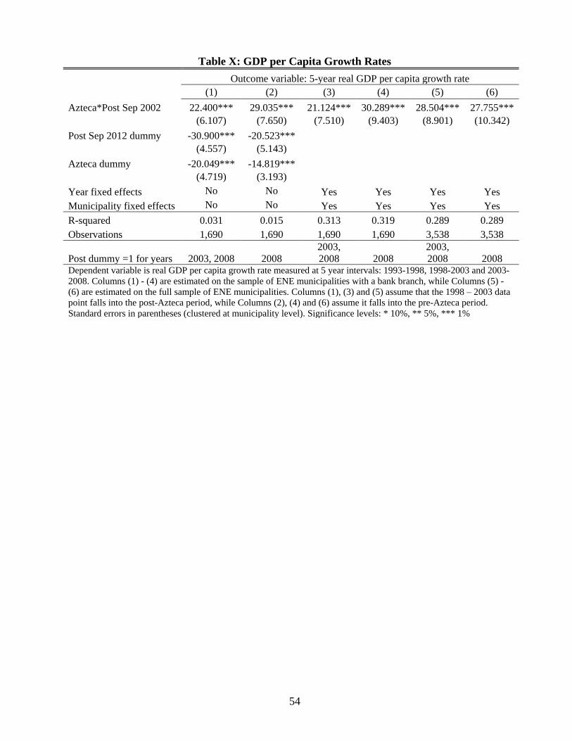
54
Table X: GDP per Capita Growth Rates
Outcome variable: 5-year real GDP per capita growth rate
(1) (2) (3) (4) (5) (6)
Azteca*Post Sep 2002 22.400*** 29.035*** 21.124*** 30.289*** 28.504*** 27.755***
(6.107) (7.650) (7.510) (9.403) (8.901) (10.342)
Post Sep 2012 dummy -30.900*** -20.523***
(4.557) (5.143)
Azteca dummy -20.049*** -14.819***
(4.719) (3.193)
Year fixed effects No No Yes Yes Yes Yes
Municipality fixed effects No No Yes Yes Yes Yes
R-squared 0.031 0.015 0.313 0.319 0.289 0.289
Observations 1,690 1,690 1,690 1,690 3,538 3,538
Post dummy =1 for years 2003, 2008 2008
2003,
2008 2008
2003,
2008 2008 Dependent variable is real GDP per capita growth rate measured at 5 year intervals: 1993-1998, 1998-2003 and 2003-
2008. Columns (1) - (4) are estimated on the sample of ENE municipalities with a bank branch, while Columns (5) -
(6) are estimated on the full sample of ENE municipalities. Columns (1), (3) and (5) assume that the 1998 – 2003 data
point falls into the post-Azteca period, while Columns (2), (4) and (6) assume it falls into the pre-Azteca period.
Standard errors in parentheses (clustered at municipality level). Significance levels: * 10%, ** 5%, *** 1%

55
Internet Appendix for “The Real Impact of Improved Access to Finance: Evidence
from Mexico”#
Table AI. Comparison of Financial Ratios for Banco Azteca and MFIs in Mexico
2004 2005 2006 2007 2008 2009 2010 2011 Average
Azteca
NPL 2.5 3.5 4.0 9.9 10.0 9.3 6.2 4.1 6.2
Interest rate 38.3 39.5 38.1 39.1 41.5 44.7 40.8 41.5 40.4
Operating
expenses 11.3 10.2 9.7 9.1 11.0 11.4 11.6 16.2 11.3
Compartamos
NPL 0.6 1.2 1.1 2.7 1.7 2.3 2.0 3.9 1.9
interest rate 88.3 85.7 80.8 78.4 81.9 72.8 71.1 71.3 78.8
Operating
expenses 29.8 30.1 29.3 28.9 30.2 25.6 27.6 29.4 28.8
Other MFI
NPL 3.8 8.6 6.7 5.5 8.5 9.7 6.7 6.5 7.0
Interest rate 58.3 63.2 66.3 63.4 76.2 68.4 71.2 75.9 67.9
Operating
expenses 33.5 35.1 35.4 34.7 39.7 38.4 37.6 39.3 36.7
The data on Azteca come from the CNBV and the data on MFI’s come from
MIXmarket.org. Operating expenses are measured as non-interest expenses over assets,
interest rate is the ratio of interest income and fee income on loans to total loans, and NPL is
the ratio of problem loans to total loans. Microfinance loan size is average for all
microfinance institutions available on MIXmarket.org. All data represent percentages.
# Citation format: Bruhn, Miriam and Inessa Love, 2013, Internet Appendix to “The Real Impact of Improved
Access to Finance: Evidence from Mexico,” Journal of Finance [vol #], [pages],
http://www.afajof.org/IA/[year].asp. Please note: Wiley-Blackwell is not responsible for the content or
functionality of any supporting information supplied by the authors. Any queries (other than missing material)
should be directed to the authors of the article.

56
Table AII: Results for the Full Sample of Municipalities
Table below presents our main results using the full sample of municipalities (i.e. including
those without any bank branch, which were excluded in the main analysis).
Dependent variable:
Informal
business
owner
dummy
Formal
business
owner
dummy
Wage-
earner
dummy
Not
employed
dummy
Log (1+
income)
(1) (2) (3) (4) (5)
Full sample 0.0070*** -0.0018 0.0013 -0.0064** 0.0409*
(No. of obs. 5,395,191) (0.0019) (0.0015) (0.0027) (0.0026) (0.0220)
Sample split by income
Above median income 0.0064** -0.0036 -0.0028 (i) -0.0013
(No. of obs. 2,631,723) (0.0027) (0.0028) (0.0034)
(0.0046)
Below median income 0.0092*** -0.0013 0.0054* -0.0133*** 0.092***
(No. of obs. 2,549,033) (0.0026) (0.0011) (0.0032) (0.0040) (0.0229)
Sample split by pre-Azteca bank branches per 100,000 people (2002-III)
Above 75th
percentile -0.0030 -0.0007 -0.0006 0.0044 0.0111
(No of obs. 2,647,366) (0.0064) (0.0041) (0.0102) (0.0090) (0.0823)
Below 75
th percentile 0.0082*** -0.0019 0.0009 -0.0072** 0.051*
(No of obs. 2,747,825) (0.0022) (0.0018) (0.0033) (0.0033) (0.0267)
Full sample regressions include all 1,218 municipalities that are covered in the labor market survey
(ENE). The median income is 1,505 pesos. The 75th percentile of bank branches per 100,000 people
across municipalities in 2002-III is 9.37. Reported are coefficients on the interaction term between the
Azteca dummy and a post September 2002 dummy. Standard errors in parentheses (clustered at
municipality level). Regressions include quarter and municipality fixed effects, as well as individual level
control variables, and the Azteca dummy interacted with a time trend. Individual level control variables
are gender, age, marital status, and education dummies. Significance levels: * 10%, ** 5%, *** 1%.
(i) Everybody is employed.

57
Table AIII: Pre-Azteca Comparison of Control Variables
Municipalities
with an Azteca
branch in Dec
2002
Municipalities
without Azteca, but
with other branch in
Dec 2002
Difference
(Azteca –
non-Azteca)
Control Variables Levels (1) (2) (3)
Female dummy 0.5318 0.5326 -0.0008
(0.4990) (0.4989) (0.0036)
Married dummy 0.6837 0.7230 -0.0392***
(0.4650) (0.4475) (0.0069)
Age 37.0602 37.6065 -0.5462***
(12.0026) (12.2543) (0.1552)
Primary education dummy 0.2277 0.2573 -0.0296***
(0.4194) (0.4372) (0.0086)
Secondary education dummy 0.2355 .2017132 0.0338***
(0.4243) .4012799 (0.0095)
High school education dummy 0.2309 0.1473 0.0836***
(0.4214) (0.3544) (0.0132)
University education dummy 0.1404 0.0780 0.0624***
(0.3474) (0.2682) (0.01111)
Control Variables Changes
Female change 0.0005 -0.0033 0.0038***
(0.0246) (0.0362) (0.0014)
Married change -0.0037 0.0007 -0.0044**
(0.0432) (0.0570) (0.0022)
Age change 0.2804 0.2426 0.0378
(1.0331) (1.3591) (0.0534)
Primary education change -0.0006 0.0021 -0.0027
(0.0369) (0.0544) (0.0021)
Secondary education change 0.0073 0.0062 0.0012
(0.0416) (0.0484) (0.0020)
High school education change 0.0027 0.0030 -0.0003
(0.0328) (0.0399) (0.0016)
University education change 0.0044 0.0012 0.0031**
(0.0263) (0.0333) (0.0013)
Columns (1) and (2) report group means for each variable with standard errors in parentheses. Column
(3) reports the t-test for differences in the means, with standard errors clustered at the municipality
level. The employed include wage earners and self-employed/business owners. Changes are changes in
ENE municipality averages from one quarter to the same quarter of the next year, using data from
2000-II to 2002-III Significance levels: * 10%, ** 5%, *** 1%

58
Table AIV: Gradual Effect of Azteca Opening
Table below reproduces our main results with an additional interaction term with a dummy
for year 2004 to test whether the effect in 2004 is larger than the effect in 2003.
Dependent variable:
Informal
business
owner
dummy
Formal
business
owner
dummy
Wage-
earner
dummy
Not
employed
dummy
Log (1+
income)
(1) (2) (3) (4) (5)
Azteca*Post Sep 2002 0.0060** -0.0014 0.0060 -0.0106*** 0.0806***
(0.0028) (0.0021) (0.0040) (0.0036) (0.0293)
Azteca*Post Sep 2002* 0.0020 -0.0001 0.0076 -0.0095** 0.0369
Year 2004 (0.0030) (0.0025) (0.0047) (0.0042) (0.0316)
R-squared 0.069 0.051 0.140 0.230 0.280
No. of observations 4,728,268 4,728,268 4,728,268 4,728,268 4,533,848 Reported are coefficients on the interaction term between the Azteca dummy and a post September 2002
dummy. Standard errors in parentheses (clustered at municipality level). Regressions include quarter and
municipality fixed effects, as well as individual level control variables, and the Azteca dummy interacted
with a time trend. Individual level control variables are gender, age, marital status, and education dummies.
Significance levels: * 10%, ** 5%, *** 1%.

59
Table AV: Falsification Test using Pre-Azteca Data Only
Table below assumes different placebo opening dates using pre-Azteca data.
Dependent variable:
Informal
business
owner
dummy
Formal
business
owner
dummy
Wage-
earner
dummy
Not
employed
dummy
Log (1+
income)
(1) (2) (3) (4) (5)
Assumed quarter of
Azteca opening
2001-II -0.0031 -0.0003 -0.0033 0.0067** -0.0366
(0.0024) (0.0016) (0.0036) (0.0033) (0.0244)
2001-III -0.0035 0.0012 -0.0012 0.0036 0.0077
(0.0028) (0.0012) (0.0040) (0.0041) (0.0300)
2001-IV 0.0043 -0.0002 0.0036 -0.0076* 0.0387
(0.0030) (0.0019) (0.0043) (0.0042) (0.0299)
Observations 2,785,598 2,785,598 2,785,598 2,785,598 2,686,266 Regressions include only pre-Azteca data, from 2000-II to 2002-III. We ran our main regressions
assuming that Azteca opened in different quarters about a year before Azteca actually opened. Reported
are coefficients on interaction term between the Azteca dummy and a post Azteca opening dummy.
Standard errors in parentheses (clustered at municipality level). Regressions include quarter and
municipality fixed effects, as well as individual level control variables and a time trend interacted with the
Azteca dummy. Individual level control variables are gender, age, marital status, and education dummies.
Significance levels: * 10%, ** 5%, *** 1%.
Top Related