


Languages
Pages
Legal


1
The Pragmatic Theory solution to the Netflix Grand Prize
Martin Piotte
Martin Chabbert
August 2009
Pragmatic Theory Inc., Canada
Table of Contents 1 Introduction ............................................................................................................................................................................ 3
2 Common Concepts .................................................................................................................................................................. 4
2.1 Time variables ............................................................................................................................................................... 4
2.2 Baselines ........................................................................................................................................................................ 4
2.2.1 Baseline1 .................................................................................................................................................................. 5
2.2.2 Baseline2 .................................................................................................................................................................. 5
2.3 Non-linear envelopes .................................................................................................................................................... 6
2.4 Parameter selection ...................................................................................................................................................... 7
2.4.1 Nelder-Mead Simplex Method ................................................................................................................................. 8
2.4.2 Assisted manual selection ........................................................................................................................................ 8
2.4.3 APT2 .......................................................................................................................................................................... 8
2.4.4 Manual selection with hint ....................................................................................................................................... 8
2.4.5 Manual .................................................................................................................................................................... 10
2.4.6 Blend optimization.................................................................................................................................................. 10
2.5 Regularized metrics ..................................................................................................................................................... 10
2.6 Iterative training .......................................................................................................................................................... 11
3 Models .................................................................................................................................................................................. 12
3.1 BK1/BK2 integrated models ........................................................................................................................................ 12
3.2 BK3 integrated model .................................................................................................................................................. 15
3.3 BK4 integrated model .................................................................................................................................................. 17
3.4 BK5 SVD++ model ........................................................................................................................................................ 24
3.5 Other integrated model variants ................................................................................................................................. 26
3.6 Matrix Factorization 1 model ...................................................................................................................................... 30
3.7 Matrix Factorization 2 model ...................................................................................................................................... 35
3.8 Usermovie model ........................................................................................................................................................ 38
3.9 SVDNN model .............................................................................................................................................................. 39
3.10 BRISMF ........................................................................................................................................................................ 39
3.11 Restricted Boltzmann Machines .................................................................................................................................. 39
3.11.1 Basic RBM models .............................................................................................................................................. 39
3.11.2 Time RBM models .............................................................................................................................................. 40
3.11.3 Decomposed RBM models ................................................................................................................................. 41
3.11.4 Split RBM model ................................................................................................................................................ 42
3.12 Asymmetric models ..................................................................................................................................................... 42
3.12.1 Asymmetric 1 model .......................................................................................................................................... 42
3.12.2 Asymmetric 3 model .......................................................................................................................................... 43
3.12.3 Asymmetric 4 model .......................................................................................................................................... 44
3.12.4 Milestone model ................................................................................................................................................ 44
3.13 Global Effects ............................................................................................................................................................... 46
3.14 Basic statistics .............................................................................................................................................................. 47

2
3.15 Non-linear post-processing model .............................................................................................................................. 47
3.16 Clustering model ......................................................................................................................................................... 48
3.17 Classification models ................................................................................................................................................... 49
3.17.1 Logistic transformation models ......................................................................................................................... 50
3.17.2 Blending classification models ........................................................................................................................... 51
3.17.3 Making predictions using classification ............................................................................................................. 51
3.18 Per-user linear regression ........................................................................................................................................... 52
3.19 KNN1 ........................................................................................................................................................................... 53
3.19.1 Proximity measures ........................................................................................................................................... 53
3.19.2 Weight measure................................................................................................................................................. 56
3.19.3 Selected combinations ....................................................................................................................................... 56
3.20 KNN2-5 ........................................................................................................................................................................ 58
3.20.1 Weight computation .......................................................................................................................................... 58
3.20.2 KNN2 .................................................................................................................................................................. 59
3.20.3 KNN3 .................................................................................................................................................................. 60
3.20.4 KNN4 .................................................................................................................................................................. 60
3.20.5 KNN5 .................................................................................................................................................................. 61
3.21 Older movie neighbourhood models ........................................................................................................................... 62
3.21.1 Movie ................................................................................................................................................................. 62
3.21.2 Movie2 ............................................................................................................................................................... 62
3.21.3 Movie3 ............................................................................................................................................................... 63
3.21.4 Movie4 ............................................................................................................................................................... 64
3.21.5 Movie6 ............................................................................................................................................................... 64
3.21.6 Movie8 ............................................................................................................................................................... 65
3.21.7 Movie5 ............................................................................................................................................................... 65
3.22 User neighbourhood models ....................................................................................................................................... 66
3.22.1 User2 model....................................................................................................................................................... 66
3.22.2 Flipped model .................................................................................................................................................... 68
4 Blending ................................................................................................................................................................................ 70
4.1 Set selection ................................................................................................................................................................ 70
4.2 Neural network blending ............................................................................................................................................. 71
4.3 Multi-stage blending ................................................................................................................................................... 73
4.3.1 Multi-linear classifier .............................................................................................................................................. 74
4.3.2 Per-movie Linear classifier ...................................................................................................................................... 74
4.3.3 Neural-Network classifier ....................................................................................................................................... 75
4.3.4 Tree (or GAM) classifier .......................................................................................................................................... 75
4.3.5 Clipping ................................................................................................................................................................... 76
4.3.6 Variants ................................................................................................................................................................... 76
4.4 Variable multiplications ............................................................................................................................................... 79
5 Towards a better recommendation system .......................................................................................................................... 80
6 Acknowledgments ................................................................................................................................................................. 81
7 List of predictors ................................................................................................................................................................... 82
8 References ............................................................................................................................................................................ 92

3
1 Introduction Recommender systems give companies a way to effectively target their products and services, thus
improving their potential for revenue. These systems are also interesting from the customer standpoint
because they are presented with alternatives focused on their likes and dislikes, thus lowering the
number of unwanted propositions. One of the keys to building a good recommender system is to find
meaningful and systematic patterns in the data, in order to identify the concrete tastes of customers.
When Netflix sought out to improve their Cinematch recommender system, this is the part of their
solution that they targeted. They put together an open, online, competition where participants are given
a set of their customers’ movie ratings and are asked to predict the ratings that these customers would
give on a different set of movies. While this is not the only component that controls the quality of their
recommender system, improving the accuracy of these predicted ratings will certainly indicate that the
customers’ tastes are better captured.
Team BellKor’s Pragmatic Chaos was the first to achieve a prediction accuracy improvement of more
than 10% over Cinematch. This team is an international coalition comprised of teams BellKor, Big Chaos
and Pragmatic Theory. The joined team includes three participants from BellKor: Yehuda Koren, Robert
Bell and Chris Volinsky; two participants from Big Chaos: Andreas Töscher and Michael Jahrer; and two
participants from Pragmatic Theory, the authors of this document: Martin Piotte and Martin Chabbert.
The complete solution, as included in the winning July 26th
2009 submission which yielded a 0.8554 quiz
set RMSE, is described over three papers, one for each of the joined teams. This document presents the
solution from team Pragmatic Theory. It includes all methods and techniques, from the most innovative
and complex aspects to some of the more naive early efforts. As the name of our team implies, our
strategy in this competition was to try anything and everything; to leave no stone unturned. Although
we have always tried to choose our methods logically, some of the resulting predictors may not have a
proper theoretical or psychological grounding; they were instead selected for their contribution to the
blended prediction accuracy. Also, because of this pragmatic approach, not all of the concepts
presented here will be usable in a real world recommender system. Still, we believe that our approach
has allowed us to find original and creative ideas and to bring known algorithms to a new level, which
should, in turn, allow for significant improvement to recommendation engines.
The first section presents some general concepts that are used across multiple models. The second
section gives detailed explanations on all of the models that were included as part of the final blend,
focusing on the more crucial and innovative models. When relevant, the parameter values that were
used for each predictor instance are given. The third section presents the different blending techniques
that were used. The final section discusses how the models and techniques presented here can be used
to build a more accurate and efficient recommender system. Note that the list of all predictors, with
their respective RMSE, is provided in an annex section.
It is assumed the reader is familiar with and understands the content of the Progress Prize papers for
2007 and 2008.

4
2 Common Concepts This section describes concepts, methods and results that are reused across multiple models and
algorithms we have developed. To avoid repetition, these elements are described once here, while the
following sections simply refer to the appropriate element when needed.
2.1 Time variables
It has become obvious over the duration of the Netflix Prize competition that the date data contained
useful information for the generation of accurate models. However, values derived from the date are
often more useful than the raw date itself.
One derived value that we found most useful is the number of ratings a user has made on a given day.
We call this measure frequency, as it measures a number of events occurring in fixed amount of time.
We speculate that the usefulness of this measure comes from the fact that Netflix subscribers use the
rating interface in two different ways. Users are initially invited to rate movies they have seen in the
past to enable the recommender to learn their preference. After this initial period, users will often only
rate movies they have just seen. We believe that ratings provided immediately after having seen the
movie and ratings provided months or years afterwards have different characteristics. When a user
selects a rating, we cannot know how long ago he has seen this movie. However, the number of ratings
provided on a given day provides a hint: a large number of ratings clearly indicates that at least some of
the movies have not been seen in the immediate past1. Similarly, users initializing the system are
unlikely to rate only one movie at a time, so single ratings are a good hint that the movie was seen in the
recent past.
In addition to the frequency measure, we also use the following time related variables in different
models:
• Elapsed time between a given rating and the first rating of the user;
• Elapsed time between a given rating and the mean rating date of the user;
• Elapsed time between a given rating and the median rating date of the user;
• Elapsed time between a given rating and the first rating of the movie;
• Elapsed time between a given rating and the mean rating date of the movie;
• Elapsed time between a given rating and the median rating date of the movie;
• Absolute date value.
Time is always measured in number of days.
2.2 Baselines
Some models require a simple approximation of the ratings as an element of the model. We developed
two such simple approximations, which we called baseline1 and baseline2.
1 There is an instance in the dataset of a user rating 5446 movies in a single day. It is clearly not possible that all
these movies have been seen by a single person in the recent past.

5
2.2.1 Baseline1
In Baseline1, a rating is approximated as:
���������(, �) = � + ����������,�(�) + ����������,�() (1)
Where:
• u is the user;
• m is the movie
• baseline1 is the value of the baseline
• � is the global mean
• bbaseline1,m is a movie bias
• bbaseline1,u is a user bias
bbaseline1,m and bbaseline1,u are chosen to minimize the following expression over the training set:
� � (� − ���������(, �))� + � � + !�"�(�)# ����������,�� (�) � $�%�& �' �� + � � + !�"�()# ����������,�� ()
(2)
Where:
• r is a rating from the training set;
• �, !�, and ! are regularization parameters;
• Nm is the number of ratings of movie m;
• Nu is the number of ratings of user u.
The model is trained using alternating least squares regression for three iterations, starting with the user
parameters. This method is described in [12] Section 4. The regularization parameters were chosen
using the assisted manual selection (see Section 2.4.2) to minimize the error on the probe set:
� 0.0987708 !� 4.65075 � 0 !� 0
Note that the zero values for � and !� actually means that no regularization is applied to the movie
coefficients.
2.2.2 Baseline2
Baseline2 is similar to baseline1; however the movie bias term is multiplied by a user scale factor to
model the user rating variance:
���������(, �) = � + ����������,�(�)(1 + ����������()* + ����������,�() (3)
Where:

6
• u is the user;
• m is the movie
• baseline2 is the value of the baseline
• � is the global mean
• bbaseline2,m is a movie bias
• bbaseline2,u is a user bias
• 1+sbaseline2 is the scale applied to the movie bias
The +1 offset in the scale factor ensures the scale remains close to 1 for users with very few ratings.
sbaseline2 , bbaseline1,m and bbaseline1,u are chosen to minimize the following expression over the training set:
(� − ���������(, �))� + � � + !�"�(�)# ����������,�� (�) + � � + !�"�()# ����������,�� ()+ � � + !�"�()# ����������� ()
(4)
Where:
• r is a rating from the training set;
• �, !�, �, !�, and ! are regularization parameters;
• Nm is the number of ratings of movie m;
• Nu is the number of ratings of user u.
The model is trained using alternating least squares regression for three iterations, starting with the
movie parameters. The regularization parameters were optimized using Nelder-Mead simplex method
to minimize the error on the probe set:
� 0.00234879 !� 0.0610418 � 0.0903385 !� 4.91299 � 0.0753211 !� 3.11288
2.3 Non-linear envelopes
Model accuracy can often be improved by transforming the output through a non-linear transformation
that limits output between 1 and 5. Such a transformation has been suggested in [3], where the
transformation is a sigmoid type function limited between 1 and 5.
The principal problem with this function is that its inflection point occurs at the middle of the range, i.e.
at 3. However, this is significantly below the training data average. Better accuracy can be achieved by
shifting the inflection point, as in the following function:

7
+,(-) =./0/1 1 + 2(+3 − 1)
1 + �4�(,456)564� �7 - < +32+3 − 5 + 2(5 − +3)
1 + �4�(,456):456�7 - ≥ +3
< (5)
Where:
• +0 is a parameter defining the level of the inflection point.
+- has the following properties:
• +-(+0) = +0
• +′-(+0) = 1
• +"-(+0) = 0
We define variants by selecting different expressions for +0:
+3(-) +3 = 3 Symmetrical sigmoid type function +�(-) +3 = � Inflection point shifted to the global average �. +�(-) +3 = � + ����������,�() Inflection point shifted to a user-specific bias
based on Baseline1. +B(-) +3 = � + ����������,�(�)< ����������()< + ����������,�() Inflection point shifted to a sample specific
bias based on Baseline2.2 +C(-) +3 = ���������(, �) Inflection point shifted to Baseline2.
It is interesting to note that any "linear" model can be transformed by wrapping it through one of the
proposed envelope functions. Often, regularization that was optimized for the linear model is still
adequate for the non-linear version. For models learned through various type of gradient descent, the
increase in program complexity required to compute the derivative of the envelope function is very
small.
2.4 Parameter selection
All statistical models used in our solution require some form of meta-parameter selection, often to
reach proper regularization. We used the following methodology to select these meta-parameters.
We train all our models twice. The first time, we train our model on the training data set where the
probe set has been removed. When a model uses feedback from movies with unknown ratings, we use
the probe set and a random half of the qualifying set for the feedback. We select meta-parameters to
optimize the accuracy on the probe set.
The second pass involves retraining the model with the selected meta-parameters, after including the
probe set in the training data. The complete qualifying set is used for feedback from rated movies with
unknown ratings.
2 The intent was to use Baseline2, but the expression provided was used by mistake. +C(-) corrects this error.

8
Every time parameter selection or validation on the probe set is mentioned in this document, it always
refers to optimizing the probe set accuracy of a model or combination of models trained on data
excluding the probe set.
We experimented with several approaches to determine optimal meta-parameters.
2.4.1 Nelder-Mead Simplex Method
The simplest and most successful way of selecting meta-parameters has been to use the Nelder-Mead
Simplex Method (see [13] and [14]). It is a well known multivariable unconstrained optimization method
that does not require derivatives. The algorithm suggests meta-parameter vectors to be tested, the
model is then evaluated and the accuracy measured on the probe set. The Nelder-Mead algorithm
requires only the measured accuracy on the probe set as feedback. This is repeated until no more
significant improvement in accuracy is observed.
2.4.2 Assisted manual selection
While the Nelder-Mead Simplex Method is very simple to use and very powerful, it requires many model
evaluations, typically ten times the number of meta-parameters being selected which leads to long
execution time for large and complex models. We used different ways to manually shorten the meta-
parameter selection time:
• We reused meta-parameters values between similar models (which could be slightly sub-
optimal);
• We evaluated meta-parameters on models with smaller dimension, then reused the value found
for the larger models;
• We used some of the meta-parameters from another model, while running the Nelder-Mead on
the remaining meta-parameters.
• We used the Nelder-Mead algorithm to select a few multiplication constants we applied to the
meta-parameters selected for a different variant.
This was used only as a time saving measure. Better results can always be obtained by running the
Nelder-Mead algorithm on all meta-parameters simultaneously.
2.4.3 APT2
We also used the APT2 automatic parameter tuning described in [4] in one instance.
2.4.4 Manual selection with hint
Another approach that we experimented with applies only to models defined as a sum of multiple
terms:
�̂ = � 7�(, �, E)��F� (6)
For one such model, it is possible to extend it by multiplying each term by a factor:

9
�′G = � �1 + �� + ��"� + H�"�# 7�(, �, E)��F� (7)
Where:
• �̂ is the initial estimate
• �′G is the extended estimate
• "�is the number of movies rated by user u
• "�is the number of users rating movie m
• u, m, d are the user, movie and date
• a, b, c are coefficients assigned to each term f
The values of a, b, c are estimated by computing a linear regression to minimize the error of �′G over the
probe set. The values of a, b and c are then used as a hint on how to manually adjust the regularization
parameters used to estimate the terms 7�(, �, E).
The idea is that for the correct regularization, the values of a, b, c should be close to zero. If different
from zero, the sign of a, b, c suggests the direction the regularization should change, and gives some
idea of the change magnitude.
We can use the following example to illustrate the methodology, using the following simple model:
�̂(, �) = � I(, �)J(�, �)� (8)
Where:
• �̂(, �) is the predicted rating;
• p(u) is a vector representing latent features for each user;
• q(m) is a vector representing latent features for each movie.
The model is trained by minimizing the following error function over the rated user-movie pairs in the
dataset.
���K� = � � LM�(, �) − � I(, �)J(�, �)� N� + O � I(, �)�� + P � J(�, �)�
� Q� $�%�& �' �� (9)
When trained using alternating least squares (see [1]), we found that the best accuracy is achieved by
making Oand Pvary according to the number of observations of a given parameter:
O = !O"� + RO (10)
P = !P"� + RP (11)

10
Where:
• ! is the part that varies inversely with the number of observations;
• R is a fixed value
N is the number of observations using the parameter. In this example "�is the number of movies rated
by u, while "�is the number of users having rated m.
For the example above, the regularization hints work in the following way:
• �� > 0 suggests to decrease the value of RO and RP
• �� < 0 suggests to increase the value of RO and RP
• �� > 0 suggests to decrease the value of !O
• �� < 0 suggests to increase the value of !O
• H� > 0 suggests to decrease the value of !P
• H� < 0 suggests to increase the value of !P
Overall, we found that the Nelder-Mead algorithm is simpler to use and converges faster, but we
included a description of the hint method since it was used in part of the final submission.
2.4.5 Manual
For most of the early models, the meta-parameters were simply chosen through trial and error to
optimize (roughly) the probe set accuracy.
2.4.6 Blend optimization
The ultimate goal of the Netflix Prize competition is to achieve highly accurate rating predictions. The
strategy we have followed, which has been followed by most participants, is to blend multiple
predictions into a single, more accurate prediction. Because of this, the quality of a model or prediction
set is not determined by its individual accuracy, but by how well it improves the blended results.
Accordingly, during automatic parameter selection with the Nelder-Mead simplex method, we
sometimes used as objective function the result of a linear regression of the model being optimized with
the set of our best predictors. This induced the parameter selection algorithm to find parameters that
might not provide the best model accuracy, but would lead a better blending result. This is most helpful
with the neighbourhood models.
When this technique was used, we indicate it in the appropriate section. When not indicated,
optimization was made on the individual model accuracy.
2.5 Regularized metrics
Several of our algorithms use an estimate of a user's (or movie's) metrics, like the rating average or
standard deviation. Because of sparseness, using the user statistic without regularization is often
undesirable. We estimate a regularized statistic by adding, to the user rating set, the equivalent to n

11
ratings taken from the training set population. If we take the rating average and rating standard
deviation as example, we obtain:
�̂ = ���� + ���� + � (12)
+T = U�����VVV + ���VVV�� + � − �̂�
(13)
Where:
• �̂ is the regularized average
• +T is the regularized standard deviation;
• nu is the number of movies rated by user u;
• n is the regularization coefficient, i.e. the equivalent of drawing n typical samples from the
global population;
• �� is the average rating of the user u;
• � is the average rating of the training set;
• ���VVVis the average of the user ratings squared;
• ��VVV is the average of the training set ratings squared.
The same methodology can be used to compute regularized higher moments, like the skew, or the
fraction of ratings given as 1, 2, 3, 4 or 5, etc.
2.6 Iterative training
Model parameters are typically learned through an iterative process: gradient descent or alternating
least squares.
Typically, model parameters are seeded with zero values. If this causes a singularity (zero gradient), then
small random values are used instead. When some special seeding procedure was used, it is described in
the appropriate section.
Typically, training is performed until maximum accuracy on the probe set is obtained. When a different
stopping rule is used, for example a fixed number of iterations, it is indicated in the appropriate section.
Unless specified otherwise, L2 regularization is used for all models. It is often described as weight decay
as this is how it appears when the model is trained using gradient descent. When the method described
in Section 2.5 is used, it is referred to explicitly. Special regularization rules are specified with each
model when appropriate.

12
3 Models This section of the document describes each model included in the solution one by one. Many of these
models are very similar. Also, some of them are early versions that were naive, poorly motivated or even
simply incorrect. However, it was in the nature of the competition that the best winning strategy was to
include many of these deficient models, even if to obtain only a very small marginal improvement. We
would expect a commercial recommender system to use only the best fraction of the model presented
here, and to achieve almost the same accuracy. Note that we have not described our failed attempts.
This explains some missing algorithms in numbered model families.
3.1 BK1/BK2 integrated models
This model is an integrated model based on the model described in Section 2.3 of [2]. 3
In [2], the user latent features have a time component that varies smoothly around the average rating
date for a user. We augment this smooth variation by a parameter h(u, t) that allows for per day
variation of the time component, which can give a user-specific correction to the time-dependent latent
feature. Interestingly, it also helps to model a user that is in reality a group of two persons sharing an
account. If we assume that only one person enters ratings on a given day, then h(u, t) can act as a
selector between which of the persons is actually providing the ratings on that day.
In some instances we also added a non-linear envelope which improves accuracy, as described in the
Common Concepts section.
The model is described by the following equations:
E�W(, X)Y = Z�(X − X�[ )\] − E�W�VVVVVV
(14)
^(, �, X) = � + ��(�, XB3) + ��() + ���()E�W(, X)Y + Z����(X)+ � J�(�) LI�() + I��()(E�W(, X)Y + ℎ(, X)) + Z:I��(, X) + 1`|"()| � b�(c)d∈f(�) Q�
�+ 1`|g\(�; )| � (�(, c) − ���������(, c))d∈ij(�;�) k�,d + 1`|"\(�; )| � H�,dd∈fj(�;�)
(15)
�̂(, �, X) = l ^(, �, X) ������ �KE��+�(^(, �, X)) �K�-������ �KE��< (16)
Where:
• E�W(, X)Y is the time varying function described in [2] to model time-dependent ratings;
• k1 is a scaling factor used to stabilize the regularization, and thus allows the same regularization
parameters for similar terms of the model;
• t is the date of the rating;
3 The acronym BK was chosen as the name of a number of integrated model variants because they were inspired
from the model described by team BellKor in [2].

13
• X�[ is the mean rating date for user u;
• k4 is an exponent applied to the date deviation;
• E�W�VVVVVV is an offset added to make the mean value of E�W(, X)Y equals to zero (but in some
experiments we left devqVVVVVV = 0)
• � is the global rating average in the training data;
• t30 is the date value mapped to an integer between 1 and 30 using equal time intervals;
• bm is the movie bias (same as bi in [2]);
• bu is the user time independent bias (same as in [2]);
• bu1 is the time-dependent part of the user bias (same as bu(1)
in [2]);
• bu2 is the per-day user bias (same as bu(2)
in [2]);
• n is the length of the latent feature vectors;
• q is the movie latent feature vector of length n;
• p is the time independent user latent feature vector of length n;
• p1 is the time-dependent user latent feature vector of length n;
• p2 is the per-day user latent feature vector of length n;
• h is a per user and per day correction to E�W(, X)Y for user latent features;
• y(j) is the implicit feedback vector of length n for movie j rated by user u as in [2];
• N(u) is the set of movies rated by u, including movies for which the rating is unknown;
• Rk(m; u) is the subset of movies with known ratings by u that are among the k neighbours of
movie m;
• Nk(m; u) is the subset of movies rated by u (rating known or not) that are among the k
neighbours of movie m;
• r(u, j) is the rating given by user u to movie j;
• Baseline1 is defined in the Common Concepts section;
• wm,j is the weight given to the rating deviation from the baseline for the movie pair (m, j);
• cm,j is an offset given to the movie pair (m, j).
• +� is a non-linear function described in the Common Concepts section.
The neighbouring movies of movie m are selected as the set of movies that maximize the following
expression:
r�,d��,d��,d + !s (17)
Where:
• r�,d is the Pearson’s correlation between the ratings of movies m and j computed over users
having rated both;
• nm,j is the number of occurrences of movies m and j rated by the same user;
• !s is a shrinkage coefficient set to 100.

14
The parameters are learned through stochastic gradient descent by minimizing the squared error over
the training set. The training samples for each user are sorted by date, so that earlier dates are
evaluated first during training. bm, bu, bu1 and bu2 are trained using a learning rate t� and a weight decay
of u. q, p, p1, p2 and y are trained using a learning rate t� and a weight decay of v. w and c are trained
using a learning rate tB and a weight decay of w. h is trained using a learning rate tx and a weight decay
of x. t values are decreased by a factor Δt at each iteration, i.e. t values are multiplied by (1 - Δt). All
the meta-parameters are selected by validation on the probe set. The values were selected using a
combination of manual selection, APT2 (described in [4]) and Nelder-Mead Simplex Method. During the
selection of the meta-parameters, the maximum number of iterations is limited to 30.
The following table shows the combinations used in the solution. Many of these models differ only in
their regularization parameters, because they were intermediate steps in the search for optimal meta-
parameters. We found that keeping some of these intermediate attempts provided a small
improvement to the blend. Note that, in all these variants, p2 is forced to zero.
Variant n k +� E�W�VVVVVV k1 k2 k4 k5 Δt
bk1-a504 50 n/a no 0 0.0363636 0.909091 0.4 1 0.0785714
bk1-a50-2 50 n/a no 0 0.0363636 0.909091 0.4 1 0.0785714
bk1-a200 200 n/a no 0 0.0363636 0.909091 0.4 1 0.0785714
bk1-a1000 1000 n/a no mean 0.0363636 0.909091 0.4 1 0.0785714
bk1-b200-1 200 300 no 0 0.04 1 0.4 1 0.1
bk1-b200-2 200 300 no 0 0.0363636 0.909091 0.4 1 0.0785714
bk1-b200-5 200 300 no mean 0.0341776 1.07444 0.4 1 0.085444
bk1-b200-6 200 300 no mean 0.0362749 0.951543 0.4 1 0.0845112
bk1-b1000 1000 300 no mean 0.0362749 0.951543 0.4 1 0.0845112
bk1-c200 200 1000 no mean 0.0362749 0.951543 0.4 1 0.0845112
bk2-b200h 200 300 no mean 0.0425157 0.994899 0.4 1 0.0918146
bk2-b200hz 200 300 yes mean 0.0425157 0.994899 0.4 1 0.0918146
Variant u v w x t� t� tB tx
bk1-a50 0 0.015 0 0 0.007 0.007 0 0
bk1-a50-2 0 0.015 0 0 0.007 0.007 0 0
bk1-a200 0 0.015 0 0 0.007 0.007 0 0
bk1-a1000 0 0.015 0 0 0.007 0.007 0 0
bk1-b200-1 0.005 0.015 0.015 0 0.007 0.007 0.001 0
bk1-b200-2 0 0.015 0.015 0 0.007 0.007 0.001 0
bk1-b200-5 0.0042722 0.0138561 0.0218166 0 0.00598108 0.0074641 0.00085444 0
bk1-b200-6 0.000330738 0.0159766 0.031863 0 0.00753674 0.00774446 0.000152311 0
bk1-b1000 0.000330738 0.0159766 0.031863 0 0.00753674 0.00774446 0.000152311 0
bk1-c200 0.000330738 0.0159766 0.031863 0 0.00753674 0.00774446 0.000152311 0
bk2-b200h 0.00342766 0.0141807 0.0256555 0.000373603 0.00765716 0.00770752 0.000134346 0.0406664
bk2-b200hz 0.00342766 0.0141807 0.0256555 0.000373603 0.00765716 0.00770752 0.000134346 0.0406664
Learning p2 simultaneously with all other parameters requires a huge amount of memory storage.
Typically, this cannot be done in a home computer main memory, and disk storage must be used.
Instead of doing this, we used the following alternative. We first train the model without the p2 term.
After convergence, the model is retrained using the movie parameters learned during pass #1 and
learning only the user parameters including p2 this time in pass #2. The idea is that during pass #2, the
4 Due to a bug, sorting of the training sample per date was incorrect for this variant.

15
users become independent from each other (since the movie parameters are now fixed), and thus is
necessary to store the p2 values only for one user at a time.
The following table shows the retraining parameters for the sets included in the solution:
Variant Pass #1 k5 Δt x t� t� tx
bk1-a50-2x bk1-a50-2 0.901726 0.0743765 0.00219152 0.00861301 0.00636511 0.0235341
bk1-a200x bk1-a200 0.901726 0.0743765 0.00219152 0.00861301 0.00636511 0.0235341
bk1-a1000x bk1-a1000 0.901726 0.0743765 0.00219152 0.00861301 0.00636511 0.0235341
bk1-b200-5x bk1-b200-5 0.85359 0.0837099 0.00265673 0.00805462 0.00595674 0.0209891
bk1-b200-6x bk1-b200-6 0.89084 0.0699494 0.00239747 0.00798123 0.00615092 0.021551
bk1-c200x bk1-c200 0.850717 0.0728293 0.00240786 0.00831418 0.00639189 0.0205951
3.2 BK3 integrated model
This model extends BK1/BK2 by including movie latent features that are time-dependent. The movie
bias is also modified to include a time invariant bias and a frequency dependent correction. The
frequency measure is defined in the Common Concepts section.
The model is described by the following equations:
E�W(, X)Y = Z�(X − X�[ )\] − E�W�VVVVVV (18) ^(, �, X) = � + ��(�) +��%(�, XB3) +��z(�, 7B3) + ��() + ���()E�W(, X)Y + Z����(X)+ �{J�(�) + J%,�(�, Xw) + Jz,�(�, 7w)| LI�() + I��()(E�W(, X)Y + ℎ(, X))�
�+ 1`|"()| � b�(c)d∈f(�) } + 1`|g\(�; )| � (�(, c) − ���������(, c))d∈ij(�;�) k�,d
+ 1`|"\(�; )| � H�,dd∈fj(�;�)
(19)
�̂(, �, X) = l ^(, �, X) ������ �KE��+�(^(, �, X)) �K� − ������ �KE��< (20)
Where:
• E�W(, X)Y is the time varying function described in [2] to model time-dependent ratings;
• k1 is a scaling factor used to stabilize the regularization, and thus allow the same regularization
parameters for similar terms of the model;
• t is the date of the rating;
• X�[ is the mean rating date for user u;
• k4 is an exponent applied to the date deviation;
• E�W�VVVVVV is an offset added to make the mean value of E�W(, X)Y equals to zero;
• � is the global rating average in the training data;
• t30 (t8) is the date value mapped to an integer between 1 and 30 (8): mapping boundaries are
selected so that each one contains roughly the same number of samples from the data set;

16
• f30 (f8) is the frequency value mapped to an integer between 1 and 30 (8): mapping boundaries
are selected so that each one contains roughly the same number of samples from the data set;
• bm is the movie bias;
• bmt is the date dependent movie bias correction;
• bmf is the frequency dependent movie bias correction;
• bu is the user time independent bias;
• bu1 is the time-dependent part of the user bias;
• bu2 is the per-day user bias;
• q is the movie latent feature vector of length n;
• qt is the date dependent correction vector of length n for the movie latent features;
• qf is the frequency dependent correction vector of length n for the movie latent features;
• p is the time independent user latent feature vector of length n;
• p1 is the time-dependent user latent feature vector of length n;
• h is a per-day correction to E�W(, X)Y for user latent features;
• y(j) is the implicit feedback vector of length n for movie j rated by a user;
• N(u) is the set of movies rated by u, including movies for which the rating is unknown;
• Rk(m; u) is the subset of movies with known ratings by u that are among the k neighbours of
movie m;
• Nk(m; u) is the subset of movies rated by u (rating known or not) that are among the k
neighbours of movie m;
• r(u, j) is the rating given by user u to movie j;
• Baseline1 is defined in the Common Concepts section;
• wm,j is the weight given to the rating deviation from the baseline for the movie pair (m, j);
• cm,j is an offset given to the movie pair (m, j).
• +� is a non-linear function described in the Common Concepts section.
The neighbouring movies are selected as in BK1/BK2.
The parameters are learned through stochastic gradient descent by minimizing the squared error over
the training set. The training samples for each user are sorted by date. bm, bmt, bmf, bu, bu1 and bu2 are
trained using a learning rate t� and a weight decay of u. q, p, p1, p2 and y are trained using a learning
rate t� and a weight decay of v. qt is trained using a learning rate t�� and a weight decay of ��. qf is
trained using a learning rate t�� and a weight decay of ��. w and c are trained using a learning rate tB
and a weight decay of w. h is trained using a learning rate tx and a weight decay of x. t values are
decreased by a factor Δt at each iterations. All the meta-parameters are selected by validation on the
probe set. The values were selected using a combination of manual selection and the Nelder-Mead
Simplex Method. During the selection of the meta-parameters, the maximum number of iterations is
limited to 30.
The following table shows the combinations used in the solution.

17
Variant n k +� k1 k2 k4 Δt
bk3-a0z 0 n/a yes 0.0362749 0.951543 0.4 0.0845112
bk3-a50 50 n/a no 0.042979 1.0 0.4 0.11587
bk3-b200 200 300 no 0.042979 1.0 0.4 0.11587
bk3-c50 50 n/a no 0.036 1.0 0.4 0.085121
bk3-c50x5 50 n/a no 0.0362749 0.951543 0.4 0.0845112
bk3-c1006 100 n/a no 0.0362749 0.951543 0.4 0.0845112
bk3-d200 200 300 no 0.0362749 0.951543 0.4 0.0845112
bk3-d200z 200 300 yes 0.0362749 0.951543 0.4 0.0845112
Variant u v w t� t� tB
bk3-a0z 0.000330738 0 0 0.00753674 0 0
bk3-a50 0.00138669 0.0092125 0 0.00790541 0.00525646 0
bk3-b200 0.00138669 0.0092125 0.030711 0.00790541 0.00525646 0.000199005
bk3-c50 0.0010603 0.0192911 0 0.00747126 0.00733103 0
bk3-c50x 0.000330738 0.0192911 0 0.00753674 0.00733103 0
bk3-c100 0.000330738 0.0192911 0 0.00753674 0.00733103 0
bk3-d200 0.000330738 0.0192911 0.031863 0.00753674 0.00733103 0.000152311
bk3-d200z 0.000330738 0.0192911 0.031863 0.00753674 0.00733103 0.000152311
Variant x �� �� tx t�� t��
bk3-a0z 0 0 0 0 0 0
bk3-a50 0.000373603 0.0092125 0 0.0406664 0.00525646 0
bk3-b200 0.000373603 0.0092125 0 0.0406664 0.00525646 0
bk3-c50 0.000373603 0.040012 0.0216398 0.0406664 1.48091x10⁻⁵
0.000106117
bk3-c50x 0.000373603 0.040012 0.0216398 0.0406664 1.48091x10⁻⁵
0.000106117
bk3-c100 0.000373603 0.040012 0.0216398 0.0406664 1.48091x10⁻⁵
0.000106117
bk3-d200 0.000373603 0.040012 0.0216398 0.0406664 1.48091 x10⁻⁵
0.000106117
bk3-d200z 0.000373603 0.040012 0.0216398 0.0406664 1.48091 x10⁻⁵
0.000106117
3.3 BK4 integrated model
This model is our most sophisticated time-dependent integrated model. It uses a very rich time
modeling and precise regularization.
One of the significant differences of this model compared to the BK1/BK2/BK3 is that several time
effects are modeled as low rank matrix factorizations. For example, a time-dependent user bias bu(u, t)
can be approximated as the inner-product of a user vector and a time vector.
Another significant difference is the introduction of a time-dependent scale factor s(u, t) inspired from
[9]. Scaling is important to capture the difference in rating behaviour from different users. Some users
will rate almost all movies with the same rating, while other will use the full scale more uniformly. Terms
in the model that include only movie and time cannot reflect this spectrum of behaviour unless they are
scaled by a user-specific parameter. These include the movie bias, the implicit feedback contribution to
5 This variant uses the 2006 ratings from the KDD cup
(http://www.netflixprize.com/community/viewtopic.php?pid=6555) 6 This variant is not used in the solution, but it is included here because it is referred to in the Logistic
Transformation section.

18
the latent features and the implicit feedback contribution of the neighbourhood model. It is important
to note that the same scale value is used for all three. The other terms do not require explicit scaling as
they already contain an implicit per-user scaling factor.
The time-dependent latent features are weighted by a sigmoid function in this model, which offers the
advantage of being restricted to [0, 1]. This sigmoid function is offset for each user so that the
expression has a mean of zero for the user or movie it applies to. The sigmoid captures the main time-
dependent correction, but it is used in conjunction with a finer grain correction term. It is interesting to
note that even the implicit feedback vector y also becomes date dependent in the model (see also
Section 3.12.4 Milestone).
The neighbourhood part is modified to underweight ratings far apart in time.
The model is defined by the following equations:
^(, �, X) = � + ��(, X) + ��(�, X) �(, X)+ �<J�(�, X)< LI�(, X) + �(, X)`|"()| � b�(c, X)d∈f(�) Q�
�+ � k~(�, c)(�(, c) − ���������(, c))d∈ij(�;�)
k�,d+ � k�(�, c)�(, X)H�,dd∈fj(�;�)
(21)
��(, X) = ��3() + � ���,�()���� {��z,�(7) + ��%,�(X�)| + ���(, X) (22)
��(�, X) = ��3(�) + � ���,�(�)���� {��z,�(7) + ��%,�(X�)| (23)
�(, X) = 1 + �3() + � ��,�()���� {�z,�(7) + �%,�(X�)| + ��(, X) (24)
J(�, X) = J3(�) + J�(�){+(7!P + RP* + J%(�, XBu) + Jz(�, 7Bu)| (25) I(, X) = I3() + I�(){+(X�!O + RO* + I�(, X)| (26) b(c, X) = b3(c) + b�(c){+(7!' + R'* + b%(c, XBu) + bz(c, 7Bu)| (27) +(-) = 11 + �4, (28)
k~(�, c) = 11 + R~X∆(�, c)U∑ � 11 + R~X∆(�, �)#��∈ij(�;�)
(29)
k�(�, c) = 11 + R~X∆(�, c)U∑ � 11 + R~X∆(�, �)#��∈fj(�;�)
(30)

19
�̂(, �, X) = .01 ^(, �, X) ������ �KE��+�(^(, �, X))+B(^(, �, X)) �K� − ������ �KE���K� − ������ �KE��+C(^(, �, X)) �K� − ������ �KE��
< (31)
Where:
• ^(, �, X) is the linear approximation of the user u rating for movie m at time t;
• � is the global rating average in the training data;
• bu(u, t) is the time-dependent user bias;
• bm(m, t) is the time-dependent movie bias;
• s(u, t) is the time-dependent scale factor for user u;
• q(m, t) is the time-dependent movie latent feature vector of length n;
• p(u, t) is the time-dependent user latent feature vector of length n;
• y(j, t) is the time-dependent implicit feedback vector of length n for movie j;
• N(u) is the set of all movies rated by u, including movies for which the rating is unknown;
• Rk(m; u) is the subset of movies with known ratings by u that are among the k neighbours of
movie m;
• Nk(m; u) is the subset of movies rated by u (rating known or not) that are among the k
neighbours of movie m;
• ww(m, j) is the weight associated with the neighbourhood relation between movies m and j
rated by user u;
• r(u, j) is the rating provided by u for movie j;
• baseline2 is described in the Common Concepts section;
• wm, j is the weight given to the movie pair (m, j) to the rating deviation from the baseline;
• cm,j is an offset given to the movie pair (m, j).
• bu0(u) is the time independent user bias;
• bu1(u) is a vector of length nbu which form the user part of the low rank matrix factorization of
the time-dependent part of the user bias;
• buf and but are vectors of length nbu which form the time part of the low rank matrix factorization
of the time-dependent part of the user bias: buf is selected based on frequency, but based on the
deviation from the median date;
• f is the frequency (see the Common Concepts section for a definition);
• tu is the difference in days between the current day and the median day for the user;
• bu2 is a per user and per day user bias correction, as explained in [2];
• bm0(u) is the time independent movie bias;
• bm1(u) is a vector of length nbm which form the movie part of the low rank matrix factorization of
the time-dependent part of the movie bias;
• bmf and bmt are vectors of length nbm which form the time part of the low rank matrix
factorization of the time-dependent part of the movie bias: bmf is selected based on frequency,
bmt based on the deviation from the median date;
• tm is the difference in days between the current day and the median rating day for the movie;

20
• s0(u) is the time independent user scale;
• s1(u) is a vector of length nsu which form the user part of the low rank matrix factorization of the
time-dependent part of the user scale;
• sf and st are vectors of length nsu which form the time part of the low rank matrix factorization
of the time-dependent part of the user scale: sf is selected based on frequency, st based on the
deviation from the median date;
• s2 is a per user and per day user scale correction, similar in concept to b2;
• q0 is a vector of length n representing the time independent movie latent features;
• q1 is a vector of length n representing the time-dependent movie latent features;
• +(7!P + RP* is the weight given to q1 based on the frequency (!P and RP are constants found
by validation on the probe set), the sigmoid value is offset per movie to have a zero mean over
the movie ratings.
• qt is an adjustment to the q1 weight for a given movie within a certain date range identified by
t36;
• qf is an adjustment to the q1 weight for a given movie within a certain frequency range identified
by f36;
• t36 identifies one of 36 time intervals chosen uniformly between the first and last date of the
training data;
• f36 identifies one of 36 frequency intervals according to a logarithmic scale between 1 and 5446
(the maximum of ratings made by one user on a single day in the training data);
• p0 is a vector of length n representing the time independent user latent features;
• p1 is a vector of length n representing the time-dependent user latent features;
• +(X�!O + RO* is the weight given to p1 based on the date deviation from the user median date
(!O and RO are constants found by validation on the probe set) ), the sigmoid value is offset per
user to have a zero mean over the user ratings;
• p2 is an adjustment to the p1 weight for a given user on a given day (note that p2 is the same as h
in BK3: it is not a vector, but a weight scaling a vector, which keeps the number of free
parameters smaller);
• y0(j) is a vector of length n representing the time independent implicit feedback for movie j;
• y1(j) is a vector of length n representing the time-dependent implicit feedback for movie j;
• +(7!' + R'* is the weight given to y1 based on the frequency (!' and R' are constants found
by validation on the probe set) , the sigmoid value is offset per movie to have a zero mean over
the movie ratings;
• yt is an adjustment to the y1 weight for a given movie within a certain date range identified by t36
(the date considered here is the date of movie j);
• yf is an adjustment to the y1 weight for a given movie within a certain frequency range identified
by f36 (the date considered here is the date of movie j);
• X∆ is the absolute value of the number of days between the ratings of movies m and j (or l) in
the neighbourhood model;

21
• R~ is a constant that determines how the neighbour weight decays when X∆ increases (R~is
determined by validation on the probe set);
• +�, +B and +C are non-linear envelope functions described in the Common Concepts section.
The neighbouring movies of movie m are selected as the set of k movies that maximize the following
expression:
r�,d��,d��,d + !s (32)
Where:
• r�,d is the similarity measure described in Appendix 1 of [7];
• nm,j is the number of occurrences of movies m and j rated by the same user;
• !s is a shrinkage coefficient determined through validation on the probe set.
The parameters are learned through stochastic gradient descent by minimizing the squared error over
the training set. In some instances, the training data was sorted by date, in others it was in random
order. This model uses a very extensive number of meta-parameters to control learning rate and weight
decay (regularization). Learning rates are decreased by a factor Δt at each iteration. All the meta-
parameters are selected by validation on the probe set. The values were selected using a combination of
manual selection and the Nelder-Mead Simplex Method. During the selection of the meta-parameters,
the maximum number of iterations is limited to 30.
Parameter Learning rate Weight decay Parameter Learning rate Weight decay
bu0 t� � q0 t�: �:
bu1 t� � p0 t�u �u
but tB B y0 t�v �v
buf tC C q1 t�w �w
bu2 t: : p1 t�x �x
bm0 tu u y1 t�3 �3
bm1 tv v wm, j t�� ��
bmt tw w cm, j t�� ��
bmf tx x p2 t�B �B
s0 t�3 �3 qt t�C �C
s1 t�� �� qf t�: �:
st t�� �� yt t�u �u
sf t�B �B yf t�v �v
s2 t�C �C
We also used this model to post-process the residual of other models. In these instances, � takes the
value of the baseline model, instead of the global average.
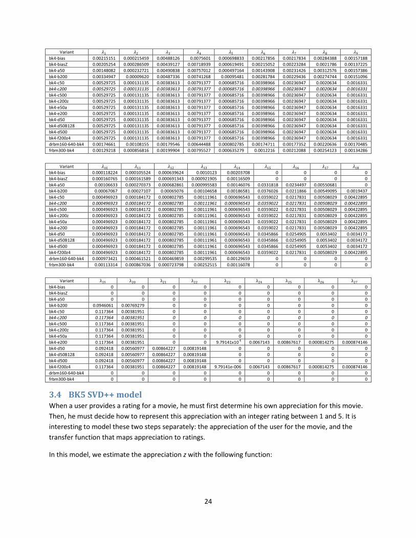
The following tables show the combinations used in the solution.

22
Variant Baseline n nbu nbm nsu k envelope sorted Δt
bk4-bias n/a 0 4 20 4 0 no no 0.0857
bk4-biasZ n/a 0 4 20 4 0 +B no 0.0857
bk4-a50 n/a 50 4 20 4 0 no no 0.0857
bk4-b200 n/a 200 4 20 4 0 no no 0.085
bk4-c50 n/a 50 4 20 4 0 no yes 0
bk4-c2008 n/a 200 4 20 4 0 no yes 0
bk4-c500 n/a 500 4 20 4 0 no yes 0
bk4-c200z n/a 200 4 20 4 0 +� yes 0
bk4-e50a n/a 50 4 20 4 0 no yes 0
bk4-e200 n/a 200 4 20 4 0 no yes 0
bk4-d50 n/a 50 4 20 4 445 no yes 0
bk4-d50B1289 n/a 50 4 20 4 445 no yes 0
bk4-d500 n/a 500 4 20 4 445 no yes 0
bk4-f200z4 n/a 200 4 20 4 445 +C yes 0
drbm160-640-bk4 drbm160-64010
0 4 20 4 0 no no 0.0857
frbm300-bk4 frbm30010
0 4 20 4 0 no no 0.0857
Variant !P !O !' RP RO R' !s R~
bk4-bias n/a n/a n/a n/a n/a n/a n/a n/a
bk4-biasZ n/a n/a n/a n/a n/a n/a n/a n/a
bk4-a50 n/a n/a n/a n/a n/a n/a n/a n/a
bk4-b200 0.121418 0.00792848 0.17656 -8.89293 220.309 11.8247 n/a n/a
bk4-c50 0.0602044 0.00689306 0.118019 -6.42095 253.658 7.21242 n/a n/a
bk4-c200 0.0602044 0.00689306 0.118019 -6.42095 253.658 7.21242 n/a n/a
bk4-c500 0.0602044 0.00689306 0.118019 -6.42095 253.658 7.21242 n/a n/a
bk4-c200z 0.0602044 0.00689306 0.118019 -6.42095 253.658 7.21242 n/a n/a
bk4-e50a 0.0602044 0.00689306 0.118019 -6.42095 253.658 7.21242 n/a n/a
bk4-e200 0.0602044 0.00689306 0.118019 -6.42095 253.658 7.21242 n/a n/a
bk4-d50 0.0539445 0.00597875 0.131885 -5.65647 228.851 7.91665 556.041 0.00147446
bk4-d50B128 0.0539445 0.00597875 0.131885 -5.65647 228.851 7.91665 556.041 0.00147446
bk4-d500 0.0539445 0.00597875 0.131885 -5.65647 228.851 7.91665 556.041 0.00147446
bk4-f200z4 0.0602044 0.00689306 0.118019 -6.42095 253.658 7.21242 556.041 0.00147446
drbm160-640-bk4 n/a n/a n/a n/a n/a n/a n/a n/a
frbm300-bk4 n/a n/a n/a n/a n/a n/a n/a n/a
7 Δtis applied only to � ... x in this variant.
8 This variant is not used in the solution, but it is included here because it is referred to in section 3.17.1 Logistic
transformation models. 9 Same as bk4-d50, but training passed the optimal score by 4 iterations to optimize blend.
10 Described later.

23
Variant t� t� tB tC t: tu tv tw tx
bk4-bias 0.00927732 0.00383994 0.00413388 0.00112172 0.00785357 0.000565172 0.00348556 0.00135257 0.000550582
bk4-biasZ 0.00949966 0.00423486 0.00408419 0.00145721 0.00893363 0.00065001 0.00399963 0.00132472 0.000584056
bk4-a50 0.00928386 0.00390146 0.00455574 0.00105276 0.00790387 0.000560385 0.00333075 0.00180471 0.000663343
bk4-b200 0.00926881 0.00386355 0.00395821 0.00110231 0.00791167 0.00062045 0.00348421 0.00144601 0.00047121
bk4-c50 0.000977427 0.00246524 0.00247907 0.00024348 0.00255845 0.000249488 0.000801197 0.000488952 0.000283411
bk4-c200 0.000977427 0.00246524 0.00247907 0.00024348 0.00255845 0.000249488 0.000801197 0.000488952 0.000283411
bk4-c500 0.000977427 0.00246524 0.00247907 0.00024348 0.00255845 0.000249488 0.000801197 0.000488952 0.000283411
bk4-c200z 0.000977427 0.00246524 0.00247907 0.00024348 0.00255845 0.000249488 0.000801197 0.000488952 0.000283411
bk4-e50a 0.000977427 0.00246524 0.00247907 0.00024348 0.00255845 0.000249488 0.000801197 0.000488952 0.000283411
bk4-e200 0.000977427 0.00246524 0.00247907 0.00024348 0.00255845 0.000249488 0.000801197 0.000488952 0.000283411
bk4-d50 0.000977427 0.00246524 0.00247907 0.00024348 0.00255845 0.000249488 0.000801197 0.000488952 0.000283411
bk4-d50B128 0.000977427 0.00246524 0.00247907 0.00024348 0.00255845 0.000249488 0.000801197 0.000488952 0.000283411
bk4-d500 0.000977427 0.00246524 0.00247907 0.00024348 0.00255845 0.000249488 0.000801197 0.000488952 0.000283411
bk4-f200z4 0.001051047 0.00265092 0.00266579 0.00026182 0.00275115 0.000268279 0.000861543 0.00052578 0.000304758
drbm160-640-
bk4
6.81554x10⁻⁵
0.00637472 0.00742226 0.00075181 0.00621834 0.000762552 0.00436458 0.00284615 0.000612556
frbm300-bk4 0.00327814 0.00637155 0.0070985 0.000263037 0.00638937 0.000652377 0.00410398 0.00275532 0.000545367
Variant t�3 t�� t�� t�B t�C t�: t�u t�v t�w
bk4-bias 0.00069273 0.00195445 0.000242657 0.00258124 0.00125313 0 0 0 0
bk4-biasZ 0.000721524 0.00218922 0.000276723 0.00260608 0.002015 0 0 0 0
bk4-a50 0.000723742 0.00192782 0.000380401 0.00201626 0.00126792 0.000579691 0.0126334 0.00134527 0
bk4-b200 0.00314745 0.00530448 0.00029168 0.00422727 0.00251472 0.00196582 0.0313884 0.00438109 0.00125546
bk4-c50 0.000756619 0.00215928 0.000134043 0.00311735 0.00111064 0.000630419 0.0111556 0.00145574 0.000583831
bk4-c200 0.000756619 0.00215928 0.000134043 0.00311735 0.00111064 0.000630419 0.0111556 0.00145574 0.000583831
bk4-c500 0.000756619 0.00215928 0.000134043 0.00311735 0.00111064 0.000630419 0.0111556 0.00145574 0.000583831
bk4-c200z 0.000756619 0.00215928 0.000134043 0.00311735 0.00111064 0.000630419 0.0111556 0.00145574 0.000583831
bk4-e50a 0.000756619 0.00215928 0.000134043 0.00311735 0.00111064 0.000630419 0.0111556 0.00145574 0.000583831
bk4-e200 0.000756619 0.00215928 0.000134043 0.00311735 0.00111064 0.000630419 0.0111556 0.00145574 0.000583831
bk4-d50 0.000756619 0.00215928 0.000134043 0.00311735 0.00111064 0.00059987 0.0122602 0.0013921 0.00062067
bk4-d50B128 0.000756619 0.00215928 0.000134043 0.00311735 0.00111064 0.00059987 0.0122602 0.0013921 0.00062067
bk4-d500 0.000756619 0.00215928 0.000134043 0.00311735 0.00111064 0.00059987 0.0122602 0.0013921 0.00062067
bk4-f200z4 0.000813608 0.00232192 0.000144139 0.00335215 0.001194293 0.000680015 0.0120332 0.00157026 0.00062976
drbm160-640-bk4 0.00164907 0.0018943 0.000674635 0.00232701 0.00113583 0 0 0 0
frbm300-bk4 0.00104467 0.00215025 0.000637943 0.00187727 0.000460018 0 0 0 0
Variant t�x t�3 t�� t�� t�B t�C t�: t�u t�v
bk4-bias 0 0 0 0 0 0 0 0 0
bk4-biasZ 0 0 0 0 0 0 0 0 0
bk4-a50 0 0 0 0 0 0 0 0 0
bk4-b200 0.0132871 0.0050094 0 0 0 0 0 0 0
bk4-c50 0.0109737 0.00186232 0 0 0 0 0 0 0
bk4-c200 0.0109737 0.00186232 0 0 0 0 0 0 0
bk4-c500 0.0109737 0.00186232 0 0 0 0 0 0 0
bk4-c200z 0.0109737 0.00186232 0 0 0 0 0 0 0
bk4-e50a 0.0109737 0.00186232 0 0 0.01319 1.48766x10⁻⁵
3.86391x10⁻⁶
0.0011758 0.000688992
bk4-e200 0.0109737 0.00186232 0 0 0.01319 1.48766x10⁻⁵
3.86391x10⁻⁶
0.0011758 0.000688992
bk4-d50 0.00984111 0.00216959 8.09761x10⁻⁵
0.000112904 0 0 0 0 0
bk4-d50B128 0.00984111 0.00216959 8.09761x10⁻⁵
0.000112904 0 0 0 0 0
bk4-d500 0.00984111 0.00216959 8.09761x10⁻⁵
0.000112904 0 0 0 0 0
bk4-f200z4 0.011837 0.00200883 7.44038x10⁻⁵
0.00010374 0.01319 1.48766x10⁻⁵
3.86391x10⁻⁶
0.0011758 0.000688992
drbm160-640-bk4 0 0 0 0 0 0 0 0 0
frbm300-bk4 0 0 0 0 0 0 0 0 0
24
Variant � � B C : u v w x
bk4-bias 0.00215151 0.000215459 0.00488126 0.0075601 0.000698833 0.00217856 0.00217834 0.00284388 0.00157188
bk4-biasZ 0.00205254 0.000286509 0.00439127 0.00718939 0.000619491 0.00215052 0.00223284 0.0021786 0.00137225
bk4-a50 0.00148082 0.000232721 0.00490838 0.00757012 0.000497164 0.00143908 0.00231426 0.00312576 0.00157386
bk4-b200 0.00334947 0.00009620 0.00487336 0.00741268 0.00095481 0.00281784 0.00229436 0.00274744 0.00151096
bk4-c50 0.00529725 0.000131135 0.00383613 0.00791377 0.000685716 0.00398966 0.00236947 0.0020634 0.0016331
bk4-c200 0.00529725 0.000131135 0.00383613 0.00791377 0.000685716 0.00398966 0.00236947 0.0020634 0.0016331
bk4-c500 0.00529725 0.000131135 0.00383613 0.00791377 0.000685716 0.00398966 0.00236947 0.0020634 0.0016331
bk4-c200z 0.00529725 0.000131135 0.00383613 0.00791377 0.000685716 0.00398966 0.00236947 0.0020634 0.0016331
bk4-e50a 0.00529725 0.000131135 0.00383613 0.00791377 0.000685716 0.00398966 0.00236947 0.0020634 0.0016331
bk4-e200 0.00529725 0.000131135 0.00383613 0.00791377 0.000685716 0.00398966 0.00236947 0.0020634 0.0016331
bk4-d50 0.00529725 0.000131135 0.00383613 0.00791377 0.000685716 0.00398966 0.00236947 0.0020634 0.0016331
bk4-d50B128 0.00529725 0.000131135 0.00383613 0.00791377 0.000685716 0.00398966 0.00236947 0.0020634 0.0016331
bk4-d500 0.00529725 0.000131135 0.00383613 0.00791377 0.000685716 0.00398966 0.00236947 0.0020634 0.0016331
bk4-f200z4 0.00529725 0.000131135 0.00383613 0.00791377 0.000685716 0.00398966 0.00236947 0.0020634 0.0016331
drbm160-640-bk4 0.00174661 0.00108155 0.00179546 0.00644488 0.000802785 0.00174711 0.00177352 0.00220636 0.00170485
frbm300-bk4 0.00129218 0.000856816 0.00199904 0.00795527 0.000635279 0.0012216 0.00212088 0.00254123 0.00134286
Variant �3 �� �� �B �C �: �u �v �w
bk4-bias 0.000118224 0.000105524 0.000639624 0.0010123 0.00203708 0 0 0 0
bk4-biasZ 0.000160765 0.000161589 0.000691343 0.000921905 0.00116509 0 0 0 0
bk4-a50 0.00106633 0.000270373 0.000682861 0.000995583 0.00146076 0.0331818 0.0234497 0.00550681 0
bk4-b200 0.00067067 0.00027107 0.00065076 0.00104658 0.00186581 0.0376026 0.0211866 0.00549095 0.0019437
bk4-c50 0.000496923 0.000184172 0.000802785 0.00111961 0.000696543 0.0359022 0.0217831 0.00508029 0.00422895
bk4-c200 0.000496923 0.000184172 0.000802785 0.00111961 0.000696543 0.0359022 0.0217831 0.00508029 0.00422895
bk4-c500 0.000496923 0.000184172 0.000802785 0.00111961 0.000696543 0.0359022 0.0217831 0.00508029 0.00422895
bk4-c200z 0.000496923 0.000184172 0.000802785 0.00111961 0.000696543 0.0359022 0.0217831 0.00508029 0.00422895
bk4-e50a 0.000496923 0.000184172 0.000802785 0.00111961 0.000696543 0.0359022 0.0217831 0.00508029 0.00422895
bk4-e200 0.000496923 0.000184172 0.000802785 0.00111961 0.000696543 0.0359022 0.0217831 0.00508029 0.00422895
bk4-d50 0.000496923 0.000184172 0.000802785 0.00111961 0.000696543 0.0345866 0.0254905 0.0053402 0.0034172
bk4-d50B128 0.000496923 0.000184172 0.000802785 0.00111961 0.000696543 0.0345866 0.0254905 0.0053402 0.0034172
bk4-d500 0.000496923 0.000184172 0.000802785 0.00111961 0.000696543 0.0345866 0.0254905 0.0053402 0.0034172
bk4-f200z4 0.000496923 0.000184172 0.000802785 0.00111961 0.000696543 0.0359022 0.0217831 0.00508029 0.00422895
drbm160-640-bk4 0.000973421 0.000461521 0.000469859 0.00299535 0.00129659 0 0 0 0
frbm300-bk4 0.00113314 0.000867036 0.000723798 0.00252515 0.00116078 0 0 0 0
Variant λ�x λ�3 λ�� λ�� λ�B λ�C λ�: λ�u λ�v
bk4-bias 0 0 0 0 0 0 0 0 0
bk4-biasZ 0 0 0 0 0 0 0 0 0
bk4-a50 0 0 0 0 0 0 0 0 0
bk4-b200 0.0946061 0.00769279 0 0 0 0 0 0 0
bk4-c50 0.117364 0.00381951 0 0 0 0 0 0 0
bk4-c200 0.117364 0.00381951 0 0 0 0 0 0 0
bk4-c500 0.117364 0.00381951 0 0 0 0 0 0 0
bk4-c200z 0.117364 0.00381951 0 0 0 0 0 0 0
bk4-e50a 0.117364 0.00381951 0 0 0 0 0 0 0
bk4-e200 0.117364 0.00381951 0 0 9.79141x10⁻⁶
0.0067143 0.00867617 0.000814275 0.000874146
bk4-d50 0.092418 0.00560977 0.00864227 0.00819148 0 0 0 0 0
bk4-d50B128 0.092418 0.00560977 0.00864227 0.00819148 0 0 0 0 0
bk4-d500 0.092418 0.00560977 0.00864227 0.00819148 0 0 0 0 0
bk4-f200z4 0.117364 0.00381951 0.00864227 0.00819148 9.79141e-006 0.0067143 0.00867617 0.000814275 0.000874146
drbm160-640-bk4 0 0 0 0 0 0 0 0 0
frbm300-bk4 0 0 0 0 0 0 0 0 0
3.4 BK5 SVD++ model
When a user provides a rating for a movie, he must first determine his own appreciation for this movie.
Then, he must decide how to represent this appreciation with an integer rating between 1 and 5. It is
interesting to model these two steps separately: the appreciation of the user for the movie, and the
transfer function that maps appreciation to ratings.
In this model, we estimate the appreciation z with the following function:

25
^ = ��(�) + � J�(�) LI�() + 1`|"()| � b�(c)d∈f(�) Q�� (33)
Where:
• ��(�) is a bias for movie m which represents the basic quality of a movie, independently from
user preferences;
• q(m) is a vector of length n representing the movie latent features;
• p(u) is a vector of length n representing the user latent features;
• N(u) is the set of all movies rated by u, including movies for which the rating is unknown;
• y(j) is a vector of length n for movie j representing the implicit feedback associated with user u
rating movie j.
We then estimate the user rating using a third degree polynomial. This allows the model to capture non-
linearity in the scale that the user chooses to express his appreciations.
�̂(, �) = �3() + (��() + 1)^ + ��()^� + �B()^B (34)
It is important to note that the +1 in (��() + 1)^ allows this term to approach z when there is
insufficient ratings for a given user to learn ��() properly.
The model is trained by minimizing the following error function through stochastic gradient descent,
using � to w as weight decays:
min�6,��,��,��,��,P,O,' �(�(, �) − �̂(, �))��,� + ���� (�) + ��J(�)�� + B�I()�� + C�b(c)�� + :�3�()+ u���() + v���() + w�B�()
(35)
The learning rates are chosen as t�for ��(�), t�for J(�), tBfor I(), tCfor b(c), t:for �3(), tufor ��(), tvfor ��()and twfor �B(). The learning rate is fixed during training. The dataset is sorted by
date for each user. All the values of and t are selected using a combination of manual selection and
Nelder-Mead simplex method. During the selection of the meta-parameters, the maximum number of
iterations is limited to 30.
We used the following parameters: n=200, t� = 0.00221326, t� = 0.00460091, tB = 0.00308307, tC = 0.000336822, t: = 0.00670341, tu = 0.00262918, tv = 0.00106459, tw = 0.000239104, � = 0.000690139, � =0.00321717, B = 0.000390205, C = 0.00153138, : = 0.000628539, u = 0.00041564, v = 0.00128092 and w = 0.00337095.
Two variants are included in the blend, which differ only by the number of iterations used.
Variant Number of iterations Comment
bk5-b200 12 Optimal score on probe set
bk5-b200B089 21 Optimal score on blended results

26
3.5 Other integrated model variants
This model is an earlier type of integrated model that proved inferior to the BKx models. It is
documented here because some variants are included in the solution. Similarly to BK4, it uses a matrix
factorization approach to model the time variant user and movie biases. It uses four time variables: the
absolute date, the elapsed time from the first rating of the user, the elapsed time from the first rating of
the movie and the frequency (number of ratings from the user on that day). All four variables are used
for both the user and movie bias, although some correlations are weak, like the impact of the elapsed
time from the first rating of the movie on the user bias.
Latent user and movie features are kept time independent, which is probably the major weakness of this
model. The neighbourhood part of the integrated model uses the factored neighbourhood approach
described in [10].
^(, �, X) = � + ��(, X) + ��(�, X) + � J�,�(�)I�,�()��� + � �J�,�(�) ��()`|"()| � b�(c)d∈f(�) ���
�+ � �JB,�(�) �B()`|g()| � k�(c)(�(, c) − ���������(, c)d∈i(�) ���
�
(36)
��(, X) = ��3() + � I�(, �)-�(X� , �)i��F� + � I�(, �)-�(X�, �)i�
�F� + � I3(, �)-3(X3, �)i6�F�
+ � Iz(, �)-z(7, �)i��F�
(37)
��(�, X) = ��3(�) + � J�(�, �)b�(X� , �)���F� + � J�(�, �)b�(X�, �)��
�F� + � J3(�, �)b3(X3, �)�6�F�
+ � Jz(�, �)bz(7, �)���F�
(38)
�̂(, �, X) = � ^ ������ �KE��+3(^) �K� − ������ �KE��+�(^) �K� − ������ �KE��<
Where:
• �̂ is the estimate for user rating movie �;
• z is the linear estimate for rating �;
• � is the global rating mean;
• bU(u, t) is the time-dependent user bias;
• bM(m, t) is the time-dependent movie bias;
• X� is the number of days between the day rated � and the first rating of ;
• X� is the number of days between the day rated � and the first movie of �;
• X3 is the absolute date of the rating;

27
• 7 is the number of ratings (frequency) made by on day X3;
• ��3() is a bias specific to ;
• ��3(�) is a bias specific to �;
• I�() is a vector of length g� for user ;
• -�(X�) is a vector of length g� for time interval X�;
• I�() is a vector of length g� for user ;
• -�(X�) is a vector of length g� for time interval X�;
• I3() is a vector of length g3 for user ;
• -3(X3) is a vector of length g3 for date X3;
• Iz() is a vector of length gz for user ;
• -z(7) is a vector of length gz for frequency 7;
• J�(�) is a vector of length �� for movie � ;
• b�(X�) is a vector of length �� for time interval X�;
• J�(�) is a vector of length �� for movie � ;
• b�(X�) is a vector of length �� for time interval X�;
• J3(�) is a vector of length �3 for movie � ;
• b3(X3) is a vector of length �3 for date X3;
• Jz(�) is a vector of length �z for movie � ;
• bz(7) is a vector of length �z for frequency 7;
• q1, q2 and q3 are the movie latent feature vectors, respectively of length n1, n2 and n3 (3 sets of
movie latent feature are used, one for regular matrix factorization, one for implicit feedback
and one for factored neighbourhood);
• p1 is the user latent feature vector of length n1;
• y(j) is the implicit feedback vector of length n for movie j;
• w(i) is the vector used in conjunction with p3 to obtain the neighbourhood weights;
• N(u) is the set of movies rated by u, including movies for which the rating is unknown;
• R(u) is the set of movies rated by u for which the rating is known;
• r(u, j) is the rating given by user u to movie j;
• Baseline1 is defined in the Common Concepts section;
• s2(u) is a scaling factor for the implicit feedback: depending on the variant, it is either chosen as
a) 1.0; b) the standard deviation of user u ratings, regularized as described in the Common
Concepts section with a population weight of 50 (σu); or c) learned through gradient descent;
• s3(u) is a scaling factor for the neighbourhood term: depending on the variant, it is either chosen
as a) 1.0; or b) learned through gradient descent;
• M(m) is the set of users having rated the movie m (used below).
The model was trained using stochastic gradient descent. The weight decay parameters
(regularization) were chosen to vary linearly with the number of movies rated by a user, or the
number of users having rated a movie, as shown below. The learning rate was changed dynamically
using the following algorithm:

28
• For each parameter, we compute the inner-product of the parameter variation during the
last two iterations. The inner-product is then normalized by dividing it by the product of the
vector lengths.
• If the result is greater than 0.5, meaning the variations were mostly collinear, than the
learning rate is increased by 20%.
• If the result is smaller than 0.5, meaning the variations were not collinear, than the learning
rate is decreased by 20%.
When the envelope is not used, convergence is accelerated by computing a least square regression on
the user parameters at each iteration. This makes a hybrid approach where the movie and time factors
are learned through gradient descent, but the user factors through linear regression.
In some variants described below, some model parameters are forced to be non-negative.
Training stopped when best accuracy was achieved on the probe set, or after 100 iterations.
Parameter Initial learning rate Weight decay Parameter Initial learning rate Weight decay ��3() 0.01 � + !�|"()| -3(X3, �) 0.000111
��
��3(�) 0.001 � + !�|�(�)| I�(, �) 0.000111
�B + !�B|"()| I�,�() 0.01 B + !B|"()| -�(X� , �) 0.000111
�B
J�,�(�) 0.001 B + !C|�(�)| I�(, �) 0.000111
�C + !�C|"()| ��() when learned 0.0001 : + !:|"()| -�(X�, �) 0.000111
�C
J�,�(�) 0.0001 : + !u|�(�)| Jz(�, �) 0.000111
�: + !�:|�(�)| b�(c) 0.0001 : + !v|�(c)| bz(7, �) 0.000111
�:
�B() when learned 0.0001 w + !w|"()| J3(�, �) 0.000111
�u + !�u|�(�)| JB,�(�) 0.0001 w + !x|�(�)| b3(X3, �) 0.000111
�u
k�(c) 0.0001 w + !�3|�(c)| J�(�, �) 0.000111
�v + !�v|�(�)| Iz(, �) 0.000111
�� + !��|"()| b�(X�, �) 0.000111
�v
-z(7, �) 0.000111
�� J�(�, �) 0.000111
�w + !�w|�(�)| I3(, �) 0.000111
�� + !��|"()| b�(X�, �) 0.000111
�w
The meta-parameters were selected using the manual selection with hint methodology described in the
Common Concepts section.
11
0.001 if non-linear envelope is used

29
Variant Envelope Non-negative n1 n2 n3 R0 RU RM Rf S0 SU SM Sf
integ0-0-0TZ σ1 n/a 0 0 0 2 2 2 4 20 20 20 40
integ0-100-100TZ σ1 n/a 0 100 100 3 3 1 6 60 20 60 120
integ0-200-200NT n/a w and q3 0 200 200 1 1 1 2 2 2 2 5
integ0-200-200TZ σ1 n/a 0 200 200 1 1 1 2 2 2 2 5
integ20-100-100NT n/a w and q3 20 100 100 1 1 1 2 2 2 2 5
integ40-200-0ST σ0 n/a 40 200 0 1 1 1 2 2 2 2 5
integ40-200-0T n/a n/a 40 200 0 1 1 1 2 2 2 2 5
integ60-0-0TS σ0 n/a 60 0 0 1 1 1 2 2 2 2 5
integ80-80-0TZM σ1 q1 80 80 0 1 1 1 2 2 2 2 5
Variant s2(u) s3(u) � !� � !� B !B !C : !: !u !v
integ0-0-0TZ n/a n/a 0.005 8 0 1 n/a n/a n/a n/a n/a n/a n/a
integ0-100-100TZ σu 1 0 6.3 0 1 n/a n/a n/a 0.005 n/a 50 0
integ0-200-200NT learned learned 0.015 5.2 0 6.7 n/a n/a n/a 0.022 0 150 75
integ0-200-200TZ σu 1 0 6.3 0 1 n/a n/a n/a 0.005 n/a 50 0
integ20-100-100NT learned learned 0.034 5.4 0 6 0.028 3 40 0.025 0 100 1012
integ40-200-0ST learned n/a 0.02 5 0 0 0.027 1.5 20 0.001 0 50 112
integ40-200-0T learned n/a 0.011 5.17 0 1.6 0.03 3 20 0.036 0 100 10012
integ60-0-0TS n/a n/a 0 6.4 0 0 0.0235 2 8 n/a n/a n/a n/a
integ80-80-0TZM 1 n/a 0.011 9 0 0 0.03 1 12 0.001 n/a 33 0
Variant w !w !x !�3 �� !�� �� !�� �B !�B
integ0-0-0TZ n/a n/a n/a n/a 0.02 2.5 0.042 0 0.023 3
integ0-100-100TZ 0.035 n/a 10 0 0.02 2.5 0.042 0 0.023 3
integ0-200-200NT 0.18 0 115 95 0.027 3.25 0.043 0.85 0.018 3.75
integ0-200-200TZ 0.035 n/a 10 0 0.01 1 0.02 1 0.01 1
integ20-100-100NT 0.165 0 100 100 0.029 3.5 0.047 1 0.022 4
integ40-200-0ST n/a n/a n/a n/a 0.011 0 0.027 0 0.012 0
integ40-200-0T n/a n/a n/a n/a 0.028 2.8 0.045 0.7 0.024 2.5
integ60-0-0TS n/a n/a n/a n/a 0.011 0.5 0.03 0 0.014 0
integ80-80-0TZM n/a n/a n/a n/a 0.012 0 0.032 0 0.013 0
Variant �C !�C �: !�: �u !�u �v !�v �w !�w
integ0-0-0TZ 0.029 4 0.001 0 0.01 1 0.01 0 0.002 60
integ0-100-100TZ 0.029 5 0.002 0 0.01 5 0.01 1 0.003 50
integ0-200-200NT 0.025 3.5 0.0003 0 0.0007 0.5 0.009 0 0.0008 20
integ0-200-200TZ 0.02 4 0.001 0 0.001 1 0.01 0 0.001 10
integ20-100-100NT 0.03 4 0.001 0 0.001 1 0.015 0 0.001 50
integ40-200-0ST 0.022 2.8 0 0 0.006 20 0.009 0 0.002 1
integ40-200-0T 0.034 2 0.001 2 0.001 10 0.013 1 0.001 20
integ60-0-0TS 0.013 8 0.001 0 0.005 5 0.008 0 0.001 0
integ80-80-0TZM 0.023 2.8 0 0 0.006 20 0.009 0 0.002 1
With this model, we experimented with a number of concepts in order to facilitate the selection of
meta-parameters (especially learning rate and regularization):
12
A value of 0 is used by mistake for movies for which the rating is unknown.

30
• By making the learning adaptable, we expected that the initial learning rate would have little
impact on the final outcome. This was relatively successful.
• The manual regularization with hints was intended to evolve into a fully automated
regularization, but we were never able to achieve this.
With hindsight, we believe that the methodology used in models BK1 to BK5 is superior:
• Select meta-parameters using the Nelder-Mead Simplex Method.
• Use a fixed learning rates, or learning rates with constant decay factors: when combined with
early stopping, this makes the usage of the αx regularization parameters unnecessary, thus
reducing the total number of parameters to be selected.
However, in this section, we documented the actual methodology used, as some of the predictions sets
were included in the solution.
3.6 Matrix Factorization 1 model
This section describes a matrix factorization method that we used earlier in the competition. It is based
on the alternating least squares matrix factorization method described in [12], but contains a number of
extensions.
The principal extension is the addition of time-dependent bias terms c, d and f. They form the equivalent
of a matrix factorization of the user-time and movie-time interaction, where the matrix rank is limited to
1.
Another extension is that we augment the user latent features with a number of fixed properties y.
These are multiplied by learned parameters z for each movie. This gives a model with a richer movie
parameterization than the user, which is desirable because movies have greater support in the data set
than users.
In this model, a rating is approximated by the following equation:
�T(, �, X) = � + �� + (H0() + E0(�)*70(X) + (H() + E(�)*7(X) + (H�() + E�(�)*7�(X�)+ �H7() + E7(�)� 77(784* + � I�()J�(�)�1
�+ � b�()^�(�)�2
�
(39)
Where:
• �̂ is the rating estimate;
• u, m and t are respectively the user, the movie and the date of the rating;
• bu is a user bias;
• bm is a movie bias;
• f0 is a function that associates each date with a learned value (the function is learned
simultaneously with the other parameters during training);

31
• c0 is the weight given to f0 for user u, which allows the model to capture the fact that ratings
may be affected by certain specific dates, like holidays;
• d0 is the weight given to f0 for movie m;
• tu is the number of days elapsed since the first rating of the user;
• fu is a function that associates each tu with a learned value (typically initialized as `X�� and
updated during training);
• cu is the weight given to fu for user u;
• du is the weight given to fu for movie m;
• tm is the number of days elapsed since the first rating of this movie;
• fm is a function which associates each tm with a learned value (typically initialized as `X�� and
updated during training);
• cm is the weight given to fm for user u;
• dm is the weight given to fm for movie m;
• f84 is the number of ratings provided by u on day t (frequency f), regrouped in 84 bins according
to a logarithmic progression (f84 takes value between 1 for a frequency of 1, and 84 for the
maximum frequency observed of 5446);
• ff is a function which associates each f84 with a learned value (typically initialized as `7� and
updated during training);
• cf is the weight given to ff for user u;
• df is the weight given to ff for movie m;
• p is a vector of length n1 representing the user latent features;
• q is a vector of length n1 representing the movie latent features;
• y is a vector of length n2 capturing a number of properties of user u. These properties are
selected before the training starts and have fixed values. We will explain below how we select
the values;
• z is a vector of length n2 that captures the weight given to each property for movie m.
The intent behind the y properties is to allow the model to have a richer representation of the movies,
which have larger support in the training date. To this end, we optionally added n2 = 59 properties to
each user y1, ..., y59 as follows:
• The square root of the user number of ratings;
• The average, variance and skew of the user ratings, regularized as described in the Common
Concepts section and using a population weight of 40;
• The fraction of the user ratings that are respectively a 1, 2, 3, 4 or 5, also regularized as
described in the Common Concepts section and using a population weight of 40;
• 50 values taken from the hidden units of the RBM model trbm50 described in Section 3.11.2
Time RBM.
The model is trained using alternating least squares regression in the following order:
1. Update user coefficients;

32
2. Update movie coefficients;
3. Update frequency function;
4. Update calendar (absolute date) function;
5. Update elapsed time from first user rating function;
6. Update elapsed time from first movie rating function.
In some variants, the time functions are left at their initial values and steps 3 to 6 are omitted. Results
are generated when there is no more accuracy improvement measured on the probe set. Training stops
after step 2 or step 6.
Regularization is best explained by using the user coefficient update as an example. When updating the
user coefficients for a specific user, all the ratings of the user are considered. Let's call X the vector
composed of the collection of all the user coefficients (bu, c0, cu, cm, cf, and p). X is found by solving the
linear problem ATAX=A
TB where A and B are determined from the non-user coefficients frozen at a
constant value during this step.
First we compute an approximation ¡ of the average of the diagonal elements of ATA over the whole
training set. All non-diagonal elements of ¡ are zero. We also compute the weighted average ¢V of X for
all users before the update is computed, where the weight corresponds to the number of ratings of each
user in the probe or qualifying set. The regularized solution for X is computed as:
¢ = ( £ + k ¡)4�( £¤ + k ¡¢V) (40)
k =∝ + �" (41)
Where α and λu are regularization constants, and N is the number of training samples included in the
evaluation of X (the number of ratings by user u for the user coefficient updates).
The same process is repeated for the movie, frequency, calendar, elapsed from first user rating and
elapsed from first movie rating coefficients. The value of w is computed similarly at all steps, the only
difference being the value of λm, λf, λ0, λtu and λtm used instead of λu for the movie, frequency, calendar,
elapsed time from first user rating and elapsed time from first movie rating respectively.
In some variants, we force all coefficients to be non-negative (see [12] figure 1 for an example of a non-
negative solver). In some others, we invert ratings (1 with 5, 2 with 4) before computing a non-negative
solution, which leads to different prediction distribution characteristics. In some variants, the bias (bu
and bm) are not used (forced to zero), as well as the values of ff, f0, fu and fm. This model is sometimes
evaluated on the residual error of another model, which is useful to introduce a time correction to
models that are not date aware.
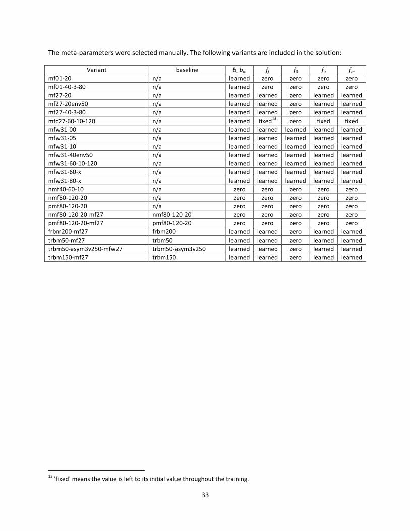
33
The meta-parameters were selected manually. The following variants are included in the solution:
Variant baseline bu bm ff f0 fu fm
mf01-20 n/a learned zero zero zero zero
mf01-40-3-80 n/a learned zero zero zero zero
mf27-20 n/a learned learned zero learned learned
mf27-20env50 n/a learned learned zero learned learned
mf27-40-3-80 n/a learned learned zero learned learned
mfc27-60-10-120 n/a learned fixed13
zero fixed fixed
mfw31-00 n/a learned learned learned learned learned
mfw31-05 n/a learned learned learned learned learned
mfw31-10 n/a learned learned learned learned learned
mfw31-40env50 n/a learned learned learned learned learned
mfw31-60-10-120 n/a learned learned learned learned learned
mfw31-60-x n/a learned learned learned learned learned
mfw31-80-x n/a learned learned learned learned learned
nmf40-60-10 n/a zero zero zero zero zero
nmf80-120-20 n/a zero zero zero zero zero
pmf80-120-20 n/a zero zero zero zero zero
nmf80-120-20-mf27 nmf80-120-20 zero zero zero zero zero
pmf80-120-20-mf27 pmf80-120-20 zero zero zero zero zero
frbm200-mf27 frbm200 learned learned zero learned learned
trbm50-mf27 trbm50 learned learned zero learned learned
trbm50-asym3v250-mfw27 trbm50-asym3v250 learned learned zero learned learned
trbm150-mf27 trbm150 learned learned zero learned learned
13
'fixed' means the value is left to its initial value throughout the training.

34
Variant n1 n2 non-negative final step α λu λm λf λ0 λtu λtm
mf01-20 20 0 no 2 50 0.01 0.01 0.01 0.01 0.01 0.01
mf01-40-3-80 40 0 no 2 80 0.03 0.03 0.03 0.03 0.03 0.03
mf27-20 20 0 no 6 50 0.01 0.01 0.01 0.01 0.01 0.01
mf27-20env50 20 59 no 6 50 0.01 0.01 0.01 0.01 0.01 0.01
mf27-40-3-80 40 0 no 6 80 0.03 0.03 0.03 0.03 0.03 0.03
mfc27-60-10-120 60 0 no 2 120 0.1 0.1 0.1 0.1 0.1 0.1
mfw31-00 0 0 no 2 50 0.01 0.01 0.01 0.01 0.01 0.01
mfw31-05 5 0 no 2 50 0.01 0.01 0.01 0.01 0.01 0.01
mfw31-10 10 0 no 2 50 0.01 0.01 0.01 0.01 0.01 0.01
mfw31-40env50 40 59 no 2 80 0.03 0.03 0.03 0.03 0.03 0.03
mfw31-60-10-120 60 0 no 2 120 0.1 0.1 0.1 0.1 0.1 0.1
mfw31-60-x 60 0 no 2 80 0.20 0.10 0.20 0.60 0.20 0.30
mfw31-80-x 80 0 no 2 90 0.40 0.17 0.21 1.00 0.14 0.10
nmf40-60-10 60 0 yes 2 60 0.1 0.1 0.1 0.1 0.1 0.1
nmf80-120-20 80 0 yes 2 120 0.2 0.2 0.2 0.2 0.2 0.2
pmf80-120-20 80 0 inverted 2 120 0.2 0.2 0.2 0.2 0.2 0.2
nmf80-120-20-mf27 80 0 yes 6 50 0.01 0.01 0.01 0.01 0.01 0.01
pmf80-120-20-mf27 80 0 inverted 6 50 0.01 0.01 0.01 0.01 0.01 0.01
frbm200-mf27 0 0 no 6 50 0.01 0.01 0.01 0.01 0.01 0.01
trbm50-mf27 0 0 no 6 50 0.01 0.01 0.01 0.01 0.01 0.01
trbm50-asym3v250-mfw27 0 0 no 2 50 0.01 0.01 0.01 0.01 0.01 0.01
trbm150-mf27 0 0 no 6 50 0.01 0.01 0.01 0.01 0.01 0.01
We also implemented a neighbourhood aware model as described in Section 4.4 of [12]. The idea
consists of re-computing the user coefficients for each prediction being made, while giving more weight
to ratings most similar to the rating being predicted. We defined two different movie proximity
measures used when re-computing user coefficients.
We also used the same logic while transposing users and movies, such that for each prediction being
made, movie coefficients are recomputed according to a user proximity measure.
The proximity measures are described by the following equations:
¦�(��, ��) = 1(1 + 0.0045§X�� − X��§* ∑ (J�(��) − J�(��)*�
J�̈VVV���
(42)
¦�(��, ��) = 1(1 + 0.0055§X�� − X��§*����(��, ��) (43)
¦B(�, �) = 1∑ (I�(�) − I�(�)*�
I�̈VVV���
(44)
���(��, ��) = 100 ���VVVVVV + ∑ (�(, ��) − �(, ��)*�� $�%��© �� ��& ��100 + ���,�� (45)
Where:
• The functions P1 and P2 represent the weight to be given to the rating of m2 when predicting m1;

35
• t«� − t«�is the time difference between the ratings of m1 and m2;
• q�VVV is the average of the squared value of the corresponding movie latent feature over all
movies;
• mse(m1, m2) is the average squared difference between the ratings of m1 and m2 rated by a
same user, the value is shrunk toward the average mean squared error (���VVVVVV ≅ 1.94).
• n«�,«� is the number of users having rated both m1 and m2;
• P3 represents the weight to be given to the rating of u2 when predicting u1.;
• I�VVV is the average of the squared value of the corresponding movie latent feature over all users.
The proximity functions P1 and P3 are based on the distance between the latent feature vectors. The
proximity function P2 is based on the mean squared error between movie ratings.
The following variants were computed. The same parameters are used as when training the regular
model, except for mfw31-80-x-m which uses α = 130 instead of α = 90.
Variant Baseline Proximity function
mf27-20-u mf27-20 P3
mf27-20env50-m mf27-20env50 P1
mfc27-60-10-120-m mfc27-60-10-120 P1
mfw31-05-m mfw31-05 P1
mfw31-40env50-m mfw31-40env50 P1
mfw31-40env50-m2 mfw31-40env50 P2
mfw31-60-10-120-m mfw31-60-10-120 P1
mfw31-80-x-m mfw31-80-x P1
nmf80-120-20-m nmf80-120-20 P1
pmf40-60-10-m pmf40-60-10 P1
drbm100-500-mfw31-m drbm100-500-mfw31 P1
frbm100-mf27-m frbm100-mf27 P1
trbm150-mf27-m trbm150-mf27 P1
3.7 Matrix Factorization 2 model
This section describes a matrix factorization method that is similar and simpler than Matrix Factorization
1. It is based on the alternating least squares matrix factorization method described in [12], but contains
a number of extensions. In this model, a rating is approximated by the following equation:
�T(, �, X) = � H�(, �, X)b�()6�=1
+ � E�(, �, X)^�(�)6�=1
+ � I�()J�(�)��
(46)
Where:
• �̂ is the rating estimate;
• u, m and t are respectively the user, the movie and the date of the rating;
• c1 is set to 1.0, so that y1 acts as a user bias;
• c2 is set to the cubic root of the time interval between t and the first rating of user u;
• c3 is set to the cubic root of the time interval between t and the first rating of movie m;
• c4 is set to the cubic root of the frequency (number of ratings made by user u on day t);

36
• c5 is set to the cubic root of the number of ratings of movie m;
• c6 is set to the average rating of m in the training data, regularized toward the global mean with
a population weight of 40 as explained in the Common Concepts section;
• y is a vector of length 6 which holds the weight given to constants c1 to c6 for user u;
• d1 is set to 1.0, so that z1 acts as a movie bias;
• d2 is set to the cubic root of the time interval between t and the first rating of user u;
• d3 is set to the cubic root of the time interval between t and the first rating of movie m;
• d4 is set to the cubic root of the frequency (number of ratings made by user u on day t);
• d5 is set to the cubic root of the number of ratings of user u;
• d6 is set to the average rating of u in the training data, regularized toward the global mean with
a population weight of 40 as explained in the Common Concepts section.
• z is a vector of length 6 which holds the weight given to constants d1 to d6 for movie m;
• p is a vector of length n representing the user latent features;
• q is a vector of length n representing the movie latent features.
The model is trained using alternating least squares regression for 30 iterations in the following order:
1. Update user coefficients;
2. Update movie coefficients.
Regularization is best explained by using the user coefficient update as an example. When updating the
user coefficients for a specific user, all the ratings of the user are considered. Let's call X the vector
composed of the collection of all the user coefficients (y and p). X is found by solving the linear problem
ATAX=A
TB where A and B are determined from the non-user coefficient frozen at a constant value during
this step.
First we compute ¡ and ¤V , the average of ATA and A
TB over the whole training set. All entries of ¡
except the diagonal entries associated with p and q are forced to zero. The regularized solution for X is
computed as:
¢ = ( £ + ! ¡ + "¯)4�( £¤ + !¤V) (47)
Where α and λ are regularization constants, and N is the number of training samples included in the
evaluation of X (the number of ratings by user u for the user coefficient updates). J is an identity matrix
where the entries corresponding to the values of y are set to zero.14
The same process is repeated for the movies (in which case N is the number of ratings of movie m).
In some variants, we force all coefficients to be non-negative. In others, some of the c or d parameters
are not used. This model is sometimes evaluated on the residual error of another model, which is useful
to introduce a time correction to models that are not date aware.
14
We are simply reporting here the regularization method used in this model. With hindsight, we find
regularization used in other models more appropriate.

37
The regularization parameters were selected manually to α = 50 and λ = 0.05. The following variants are
included in the solution:
Variant baseline Use c1d1 Use c2d2c3d3 Use c4d4 Use c5d5c6d6 n non-negative
nnmf40 n/a no no no no 40 yes
nnmf80 n/a no no no no 80 yes
ssvd-04-00 n/a yes no no no 0 no
ssvd-04-10 n/a yes no no no 10 no
ssvd-04-40 n/a yes no no no 40 no
ssvd-07-30-215
n/a yes yes no no 30 no
ssvd-31-00 n/a yes yes no yes 0 no
ssvd-31-10 n/a yes yes no yes 10 no
ssvd-31-20 n/a yes yes no yes 20 no
ssvd-31-60 n/a yes yes no yes 60 no
ssvd-39-00 n/a yes yes yes no 0 no
ssvd-39-05 n/a yes yes yes no 5 no
ssvd-39-10 n/a yes yes yes no 10 no
ssvd-63-00 n/a yes yes yes yes 0 no
ssvd-63-30 n/a yes yes yes yes 30 no
rbm100-ssvd-07-00 rbm100 yes yes no no 0 no
crbm100-ssvd-07-00 crbm100 yes yes no no 0 no
crbm100-ssvd-07-20 crbm100 yes yes no no 20 no
crbm100x-ssvd-03-00 crbm100x no yes no no 0 no
crbm200-ssvd-07-00 crbm200 yes yes no no 0 no
trbm50-ssvd-39-00 trbm50 yes yes yes no 0 no
trbm100-ssvd-31-00 trbm100 yes yes no yes 0 no
trbm150-ssvd-07-00 trbm150 yes yes no no 0 no
trbm150-ssvd-39-00 trbm150 yes yes yes no 0 no
nnmf40-ssvd-07-00 nnmf40 yes yes no no 0 no
nnmf80-ssvd-39-00 nnmf80 yes yes yes no 0 no
We also implemented a neighbourhood aware model as described in Section 4.4 of [12]. Like in Section
3.6 Matrix Factorization 1, the idea consists of re-computing the user coefficients for each prediction
being made, while giving more weight to ratings most similar to the rating being predicted. We defined
one movie proximity measure used when re-computing user coefficients. We also used the same logic
while transposing users and movies, such that for each prediction being made movie coefficients are
recomputed according to a user proximity measure.
¦�(��, ��) = 10.001 + ∑ (J�(��) − J�(��)*�
J�̈VVV��
(48)
¦�(�, �) = 10.001 + ∑ (I�(�) − I�(�)*�
I�̈VVV��
(49)
Where:
15
This variant uses α = 16 and λ = 0.02.

38
• The functions P1 represents the weight to be given to the rating of m2 when predicting m1;
• q�VVV is the average of the squared value of the corresponding movie latent feature over all
movies;
• P2 represents the weight to be given to the rating of u2 when predicting u1.;
• I�VVV is the average of the squared value of the corresponding movie latent feature over all users.
The proximity functions P1 and P2 are based on the distance between the latent feature vectors.
The following variants were computed. The same parameters are used as when training the regular
model.
Variant Baseline Proximity function
ssvd-04-10-m ssvd-04-10 P1
ssvd-04-40-m ssvd-04-40 P1
ssvd-31-10-m ssvd-31-10 P1
ssvd-31-20-m ssvd-31-20 P1
ssvd-31-20-u ssvd-31-20 P2
3.8 Usermovie model
This is a very early and simple model where the rating is modeled as the sum of a user and a movie bias
(bu and bm). The values are initialized to zero and updated using the following equations for two
iterations.
�̂(, �) = �� + ��
(50)
�� = ∑ (�(, �) − ��)�∈f(�) + !� ��VVVV(|"(�)| + !�)
(51)
�� = ∑ (�(, �) − ��)�∈f(�) + !���VVV(|"()| + !�)
(52)
Where:
• �̂(, �) is the estimated rating for user u and movie m;
• �� is the movie bias for movie m;
• �� is the user bias for user u;
• N(m) is the subset of users that have rated movie m;
• αm=20 is the movie shrinkage coefficient;
• N(u) is the subset of movies rated by user u;
• αu=8.3 is the user shrinkage coefficient;
• ��VVVV is the average of (�(, �) − ��) over the complete training set;
• �VVV is the average of (�(, �) − ��) over the complete training set.
The following table shows the variant selected in the solution:

39
Variant
usermovie
3.9 SVDNN model
This model is an early and plain version of a Matrix Factorization model (as described in [1]) where NN
represents the number of latent features used. Training is done by alternating least squares regression.
Regularization is similar to Section 3.7 Matrix Factorization 2. Let's call X the vector composed of the
user coefficients. X is found by solving the linear problem ATAX=A
TB where A and B are determined from
the movie coefficients frozen at a constant value during this step.
First we compute ¡, the average of ATA over the whole training set. All non-diagonal entries of ¡ are
forced to zero. The regularized solution for X is computed as:
¢ = ( £ + ! ¡ + "°)4� < £¤< (53)
Where α and λ are regularization constants, and N is the number of training samples included in the
evaluation of X (the number of ratings by user u for the user coefficient updates). I is the identity matrix.
The same process is repeated for the movies (in which case N is the number of ratings of movie m).
The variants that were selected in the solution were trained on the residual errors of the usermovie
model. Note that the svdNNx variant also runs an additional pass of the usermovie model on the
residuals of the svdNN model.
The following table shows the predictors selected in the solution.
Variant
svd02x
svd05x
3.10 BRISMF
We implemented the BRISMF model as described in [11]. We reused all given parameters including
number of epochs and regularization. The following table indicates the variants that were used in the
solution.
Variant Comment
brismf40 Based on BRISMF#1UM in [11]
brismf250 Based on BRISMF#250UM in [11]
brismf760 Based on BRISMF#1000UM in [11], but with rank limited to K=760.
brismf760n Based on SemPosMF#800 in [11], but with rank limited to K=760.
3.11 Restricted Boltzmann Machines
3.11.1 Basic RBM models
We implemented all the RBM types described in [5]. The following variants were included in the
solution:

40
Variant Description
rbm100 Ordinary RBM from Section 2 of [5], with 100 softmax hidden units. The model is trained using mini-
batches of 1000 users, a learning rate of 2x10⁻⁵
, a weight decay of 0.02 and a momentum of 0.9.
crbm100 Conditional RBM from Section 4 of [5], with 100 softmax hidden units. The model is trained using
mini-batches of 1000 users, a learning rate of 2x10⁻⁵
, a weight decay of 0.02 and a momentum of 0.9.
crbm100x Conditional RBM from Section 4 of [5], with 100 softmax hidden units. The model is trained using
mini-batches of 1000 users, a learning rate of 2x10⁻⁵
, a weight decay of 0.02 and a momentum of 0.9.
The learning rate is progressively reduced by a factor of 8 over the last 6 iterations.
crbm200 Conditional RBM from Section 4 of [5], with 200 softmax hidden units. The model is trained using
mini-batches of 1000 users, a learning rate of 2x10⁻⁵
, a weight decay of 0.02 and a momentum of 0.9.
drbm100-500 Conditional Factored RBM from Section 5 of [5], with a factorization of rank 100 and 500 softmax
hidden unit. The initial learning rate is set to 0.0005 for the hidden unit biases and the rank reducing
matrices, 0.005 for all others. The learning rate is reduced exponentially by a factor of 1000 over 100
iterations. Update occurs by batches of 1 user, with no weight decay or momentum.
drbm160-640 Conditional Factored RBM from Section 5 of [5], with a factorization of rank 160 and 640 softmax
hidden unit. The same training parameters were used as drbm100-500.
urbm20-1000 Conditional Factored RBM from Section 5 of [5], with a factorization of rank 20 and 1000 softmax
hidden unit. In this variant, the role of the users and the movies is reversed: each movie is modeled
by a number of units, and weights connect the hidden units to the users. The initial learning rate is
set to 4.51005x10⁻⁷
for the hidden unit biases and the rank reducing matrices, 6.21418x10⁻⁵
for all
others. The learning rate is reduced by a factor of 0.0315713 per iteration. Update occurs by batches
of 1 user, with a weight decay of 0.0946444 on all parameters except the hidden unit biases, and no
momentum. The meta-parameters were selected using the Nelder-Mead Simplex Method. During
the selection of the meta-parameters, the maximum number of iterations is limited to 100.
integ0-0-0TZ-grbm200 RBM with 200 Gaussian visible units as described in [7], running on residuals of integ0-0-0TZ. The
model is trained using mini-batches of 1000 users, an initial learning rate of 8.18119x10⁻⁵
which
decreased by a factor 0.000390623 at each iteration. A weight decay of 0.00012058 + 0.0569244/N is
used where N is the support of the respective parameter. Momentum is set to zero. The meta-
parameters were selected using the Nelder-Mead Simplex Method. During the selection of the meta-
parameters, the maximum number of iterations is limited to 100.
mfw31-10-grbm200 RBM with 200 Gaussian visible units as described in [7], running on residuals of mfw31-10. The same
training parameters were used as integ0-0-0TZ-grbm200.
3.11.2 Time RBM models
We developed a new RBM variant that we called Time RBM which takes into account the dates of the
ratings. The Time RBM is based on the Conditional RBM, except that the weights are the product of a
movie factor by a time factor.
±�d\ = �d\ ¤dz (54)
The �d\ are akin to typical RBM weights: they capture the relation between item i and hidden unit j for
rating k. The ¤dz capture the relationship between the hidden unit j and the number of ratings of this
user on that day (frequency f). The update rule becomes:
Δ �d\ = ²(³¤dzW�\ℎd´&�%� − ³¤dzW�\ℎd´�µ&��* (55)
Δ¤dz = ² M³¶� �d\ W�\�\ · ℎd´&�%� − ³¶� �d\ W�\�\ · ℎd´�µ&��N (56)

41
The biases and the conditional part do not depend on the date and are computed as in [5]. The weight
decay for the ¤dz is made toward 1.0 instead of the usual 0.0. The model is trained using mini-batches of
1000 users, a learning rate of 2x10⁻⁵, a weight decay of 0.02 and a momentum of 0.9.
Instead of using the rating frequency, we also tried using the raw date in the same way. The following
variants are included in the solution:
Variant Description
frbm100 Time RBM using frequency, with 100 softmax hidden units.
frbm200 Time RBM using frequency, with 200 softmax hidden units.
frbm200x Time RBM using frequency, with 200 softmax hidden units. Instead of using one iteration of the
mean field equation to make predictions, we use the expression defined in equation (7) of [5].
frbm300 Time RBM using frequency, with 200 softmax hidden units.
frbm300x Time RBM using frequency, with 200 softmax hidden units. Instead of using one iteration of the
mean field equation to make predictions, we use the expression defined in equation (7) of [5].
trbm50 Time RBM using date, with 50 softmax hidden units.
trbm100 Time RBM using date, with 100 softmax hidden units.
trbm150 Time RBM using date, with 150 softmax hidden units.
3.11.3 Decomposed RBM models
To generate a prediction, the classic RBM actually computes the probability that a given rating is a 1, 2,
3, 4 or 5. Typically, the prediction is selected as:
�̂ = I(� = 1) + 2I(� = 2) + 3I(� = 3) + 4I(� = 4) + 5I(� = 5) (57)
Where:
• �̂ is the prediction;
• p(r=x) is the probability that the rating takes the value x.
However, under certain circumstances, it may be better to let the blending algorithm select optimized
weights rather than the expected 1, 2, 3, 4 and 5 values. To that end, we also produce the following
expressions and generate them as prediction sets. Their individual accuracy is very poor, but they blend
well with each other and with the rest. ¸� = I(� = 2) + I(� = 3) + I(� = 4) + I(� = 5) (58) ¸� = I(� = 3) + I(� = 4) + I(� = 5) (59) ¸B = I(� = 4) + I(� = 5) (60) ¸C = I(� = 5) (61)
We included the following variants in the blend:
Variant Baseline Expression
drbm160-640g1 drbm160-640 g1
drbm160-640g2 drbm160-640 g2
drbm160-640g3 drbm160-640 g3
drbm160-640g4 drbm160-640 g4
frbm300g1 frbm300 g1
frbm300g2 frbm300 g2
frbm300g3 frbm300 g3
frbm300g4 frbm300 g4

42
3.11.4 Split RBM model
We described in the previous section (3.11.3 Decomposed RBM) that we can produce separate
prediction sets from a RBM, each set representing the probability of the rating being above a certain
threshold 1, 2, 3 or 4, using expressions g1, g2, g3 and g4. We also experimented with a variant that
tried to directly estimate one of g1, g2, g3 or g4.
We replaced the visible units with a single softmax unit per rating. The visible unit is interpreted as the
probability that the correct rating is greater than g, where g one is 1, 2, 3 or 4. The rest of the model
works as the Time RBM model using frequency.
The initial learning rate is set to γ and reduced by a factor Δγ per iteration. Update occurs by batches of
1 user, with no weight decay or momentum. The meta-parameter were selected using the Nelder-Mead
Simplex Method. During the selection of the meta-parameters, the maximum number of iterations is
limited to 100.
This provided results much inferior to the Decomposed RBMs, and they are described here only because
some variants were included in the solution:
Variant γ Δγ Comment
frbm2-100g1 0.00106641 0.0570313 Time RBM with frequency, 100 hidden units and g=1.
frbm2-100g2 0.00246875 0.0351563 Time RBM with frequency, 100 hidden units and g=2.
frbm2-100g3 0.00140625 0.00546875 Time RBM with frequency, 100 hidden units and g=3.
frbm2-100g4 0.0021875 0.0265625 Time RBM with frequency, 100 hidden units and g=4.
3.12 Asymmetric models
Asymmetric models are from a family of models that do not directly model user latent features, but
instead infer the user tastes by the movie that he rated. This was first described in [6] as NSVD1. The
name Asymmetric was used in [7] which also introduced several variations. We describe here our own
variations.
One difference in our implementation compared to Paterek's is that we don't use a bias term. Instead,
we always run the model on the residual of another model: time-dependent biases, a low rank matrix
factorization or a Restricted Boltzmann Machine.
3.12.1 Asymmetric 1 model
This variant differs from NSVD1 in [6] by an extra factor in the expression that accounts for the value of
the rating.
�̂(, �) = 1`|"()| � J�(�) � b�(c)d ∈f(�)�
�F� H(c, �d) (62)
Where:
• �̂ is the predicted rating for user u and movie m;
• N(u) is the set of ratings provided by user u, whether or not the rating is known;
• q is a vector of length n representing the movie latent features;

43
• y(j) is a vector of length n representing the implicit feedback from knowing that movie j was
rated by u;
• rj is the rating given to movie j; if not known, then rj takes the value zero;
• c is a correction factor applied according to the rating of movie j, it is a table of dimension
6xnumber of movies.
This model was trained using gradient descent with mini-batch of 1000 users, starting with a learning
rate of 0.001 which decreased by a factor of 0.25 at each iteration until the rate reached 5x10⁻⁶
. It used a
weight decay of 0.01 and a momentum of 0.9.
This model was not very successful, but it is documented here as the following variant was included in
the solution:
Variant Baseline n
ssvd-31-00-asym1-20 ssvd-31-00 20
3.12.2 Asymmetric 3 model
This variant is much closer to NSVD1 in [6]. The main difference is the introduction of a user-specific
scale s(u).
�̂(, �) = �()`|"()| � J�(�) � b�(c)d ∈f(�)�
�F� (63)
Where:
• �̂ is the predicted rating for user u and movie m;
• N(u) is the set of ratings provided by user u, whether or not the rating is known;
• q is a vector of length n representing the movie latent features;
• y(j) is a vector of length n representing the implicit feedback from knowing that movie j was
rated by u;
• s(u) is a user-specific scale, which is either the constant 1, or the value of the user ratings
standard deviation regularized with a population weight of 40 as described in the Common
Concepts section.
The model was trained using gradient descent with mini-batches of 1000 users and a learning rate which
decreased by a factor of 0.21 at each iteration, until the rate reached 10-3
of the initial value. It used a
weight decay of 0.01 and a momentum of 0.9.
In one variant, we re-compute s(u) after training as follows:
• For each user, we compute, through linear regression, the value of s(u) that would minimize the
prediction error on the training set;
• We then compute a weighted average between the old value and the new value of s(u), where
the old value gets a weight of 40, and the new value a weight equal to the number of known
ratings of user u.

44
The following variants were included in the final blend:
Variant Baseline n s(u) initial learning rate
mfw31-05-asym3v250 mfw31 250 standard deviation 0.0004
ssvd-31-00-asym3-20 ssvd-31-00 20 1.0 0.0005
ssvd-31-00-asym3-100 ssvd-31-00 100 1.0 0.0005
ssvd-31-00-asym3-200 ssvd-31-00 200 1.0 0.0005
ssvd-31-00-asym3v-300 ssvd-31-00 300 standard deviation 0.0004
ssvd-31-00-asym3w-200 ssvd-31-00 200 post-processed 0.0004
trbm50-asym3v250 trbm50 250 standard deviation 0.0004
3.12.3 Asymmetric 4 model
This variant was inspired from the sigmoid variants found in [7].
�̂(, �) = �() � J�(�)+ ��� + � b�(c)d ∈f(�) ���F� (64)
+(-) = 11 + �4, (65)
Where:
• �̂ is the predicted rating for user u and movie m;
• N(u) is the set of ratings provided by user u, whether or not the rating is known;
• q is a vector of length n representing the movie latent features;
• y(j) is a vector of length n representing the implicit feedback from knowing that movie j was
rated by u;
• b is a vector of length n representing a bias in the sigmoid function σ;
• s(u) is a user-specific scale, which is either the constant 1, or the value of the user ratings
standard deviation regularized with a population weight of 40 as described in the Common
Concepts section.
The model was trained using gradient descent with mini-batches of 1000 users and an initial learning
rate of 0.0005 which decreased by a factor of 0.21 at each iteration, until the rate reached 10-3
of the
initial value. It used a weight decay of 0.01 and a momentum of 0.9.
The following variants were included in the solution:
Variant Baseline n s(u)
ssvd-31-00-asym4-200 ssvd-31-00 200 1.0
ssvd-31-00-asym4v-200 ssvd-31-00 200 standard deviation
3.12.4 Milestone model
We named our most successful variant milestone although the name is an abuse of language. A
prediction is generated using the following model:

45
�̂(, �) = �()`"() � J(�, �) � {k(, 7d*b�(c, �) + (1 − k(, 7d*)b�(c, �)|d $�%�& �' ��� (66)
Where:
• �̂ is the predicted rating for user u and movie m;
• fj is the frequency, i.e. the number of ratings made by user u the day he rated movie j;
• s(u) is a user-specific scale, which is the value of the user ratings standard deviation regularized
with a population weight of 40 as described in the Common Concepts section;
• N(u) is the number of movies rated by u, whether or not the score is known;
• q is a vector of length n representing the movie latent features;
• y1 and y2 are also vectors of length n representing the implicit feedback of having user u rating
the associated movie;
• w is the date dependent weight applied to y1 and y2 to produce the user factors.
While Paterek in [6] created user latent factors by summing a vector for each movie rated by the user,
instead we add a linear combination of two vectors y1 and y2, weighted by w. Paterek's idea was that the
user tastes could be inferred by the identity of the movies rated by the user, without looking at the
individual score. We extended this approach by assuming that the contribution of each movie rated by
the user was a function of the date at which the rating was provided, as captured by w. The values of q,
y1 and y2 are learned through gradient descent. The values of w are chosen as one among the following
alternatives:

46
#0 k = l0 �7 7 = 11 �7 7 > 1< #3 k varies linearly from 0 to 1 over the range of frequencies observed for u.
#4
k =.//0//1
0 �7 7 = 11 4¹ �7 7 = 21 2¹ �7 7 = 33 4¹ �7 7 = 41 �7 7 > 4<
#5 k = �7 − 19 �7 7 < 101 �7 7 ≥ 10< #6 k = 11 + 110 (7 − 1)
#7 k = 11 + 120 (7 − 1)
#9 k = 11 + 1400 (7 − 1)�
The model was trained using gradient descent with mini-batches of 1000 users, with an initial learning
rate of 0.0004 which decreased by a factor of 0.21 at each iteration, until the rate reached 10-3
of the
initial value. It used a weight decay of 0.01 and a momentum of 0.9.
The following variants are included in the solution:
Variant Baseline n w
mfw31-00milestone3-100 mfw31-00 100 #3
mfw31-00milestone4-100 mfw31-00 100 #4
mfw31-00milestone5-100 mfw31-00 100 #5
mfw31-00milestone6-100 mfw31-00 100 #6
mfw31-00milestone7-100 mfw31-00 100 #7
mfw31-00milestone9-100 mfw31-00 100 #9
mfw31-10-milestone0-150 mfw31-10 150 #0
mfw31-10-milestone5-150 mfw31-10 150 #5
trbm50-milestone0-150 trbm50 150 #0
trbm50-milestone9-150 trbm50 150 #9
In our opinion, this variant of asymmetrical model supersedes the other variants presented in this
document. The other forms were described essentially because some old results were included in the
solution. The astute reader will also notice the similitude between the milestone model and the implicit
feedback component in the BK4 model.
3.13 Global Effects
We implemented Global Effects (GE) and Global Time Effects (GTE) as described in [4]. The various
parameters used were also the ones noted in [4]. The following table shows the base predictors that
were included in the solution. Note that all of these use the first 14 effects, in the order described in [4].

47
Variant Comment
globalEffect14 Global Effects.
gte14b Global Time Effects. The basic user and movie effects were run only once (as opposed
to twice, which is suggested in [4]).
3.14 Basic statistics
The basic statistics do not attempt to model the prediction, but simply reflect measures of the user and
movie statistical properties. These properties have a weak correlation with the ratings and can be useful
inputs for blending.
The main categories of statistics that were computed are support (count), mean, standard deviation and
skew. The probabilities of the ratings 2, 3, 4 and 5 were also computed. These 8 statistics were
computed both for each user and for each movie for a total of 16 predictors. Note that none of these
are regularized in any way; they are just straight statistics.
The following table indicates the predictors that were used in the solution:
Variant Comment
mmean Movie mean
mp5 Probability of the movie being rated 5
mskew Movie skew
ucount User support (number of ratings)
uskew User skew
up2 Probability of the user rating a 2
up3 Probability of the user rating a 3
up4 Probability of the user rating a 4
up5 Probability of the user rating a 5
3.15 Non-linear post-processing model
User rating distributions are most often asymmetrical. This is easy to verify by computing the skew for
the rating distribution of each user. The skew varies from very positive for users with many 1's and a few
higher ratings, to the very negative for users with many 5's and a few lower ratings. On the other hand,
most models have an essentially symmetrical formulation, which makes the predictions inaccurate in
certain rating ranges. We propose to post-process a model using a third degree polynomial to correct for
this effect.
�̂(, �) = -(, �) + �3() + ��()(-(, �) − ��) + ��()(-(, �) − ��)� + �B() (-(, �) − ��)B+ �3(�) + ��(�)(-(, �) − ��) + ��(�)(-(, �) − ��)� + �B(�) (-(, �) − ��)B (67)
Where:
• �̂(, �) is the generated prediction for user u and movie m;
• x is the model prediction being post-processed;
• a0, a1, a2, a3, b0, b1, b2 and b3 are the coefficients of the polynomial transformation learned
during training;
• �� is the average ratings of user u;

48
• �� is the average ratings of movie m;
The transformation parameters a0, a1, a2, a3, b0, b1, b2 and b3 are learned by alternating least squares
regression, starting with the movies, for two iterations.
Regularization is computed by adding the expression α + λN to the diagonal elements of the regression
matrix. α and λ are constants selected through validation on the probe set automatically, using the
Nelder-Mead Simplex Method. N is the number of training samples in this particular regression matrix
(number of movies rated by user u for the a factors, numbers of users having rated movie m for the b
factors). The values of α and λ are selected independently for each a and b, so a total of 16 meta-
parameters are trained using the Nelder-Mead algorithm.
The following variants are present in the solution:
Variant Baseline
bk1-a1000-nlpp1 bk1-a1000
bk3-d200z-nlpp1 bk3-d200z
bk4-f200z4-nlpp1 bk4-f200z4
bk3-200gx-nlpp1B10516
bk3-200gx
bk5-b200B089-nlpp1B10816
bk5-b200B089
3.16 Clustering model
Another post-processing method we developed was based on user and movie clusters. We randomly
divided the users in 256 bins. We also randomly divided the movies in 256 bins, creating 256x256=65536
clusters. We then minimize the intra-cluster rating variance by moving users and movies between bins,
while keeping the bin sizes roughly equal. This is repeated greedily, until the intra-cluster variance no
longer improves significantly. Note that the intra-cluster variance is computed on the residual error from
the ssvd-04-00 model described previously, which basically centers the data.
The idea is that the average value of the cluster is a predictor for all user/movie pairs in the cluster.
However, some of the 65536 clusters have fewer known ratings, making the cluster average value
imprecise. To improve the prediction accuracy, we redo the same clustering algorithm using only 128
movie and user bins, thus obtaining larger clusters. Similarly, we also computed 64, 32, 16, 8, 4, 2 and 1
bin clusters. The final prediction for a movie/user pair is a weighted average of the mean rating in each
cluster the movie/user pair belongs to:
�̂(, �) = � k���w
�F3 (68)
kw = "w"w + ! (69)
k� = �1 − � kdw
dF�º� � "�"� + ! , 7K� 0 < � < 8 (70)
16
This set used direct optimization of the blended score.

49
k3 = �1 − � kdw
dF� � (71)
Where:
• �̂(, �) is the prediction for user u and movie m;
• �, is the average of the cluster with 2x bins which contains the pair (u,m);
• w are the weights given to each cluster the pair (u, m) belongs to;
• Nx is the number of ratings in the cluster using 2x bins;
• α is a regularization parameter set to 20000.
The following variants are present in the solution:
Variant Baseline
ssvd-31-20-cluster ssvd-31-20
This is the only attempt at clustering that was kept in the solution. In general, we found that clustering
could not improve the more accurate models (like BK4), and had virtually no impact on the accuracy of
the final blend.
3.17 Classification models
Typically, models used for collaborative filtering attempt to fit a real-valued function to minimize the
prediction error. Most models do not exploit the knowledge that ratings take discrete values between 1
and 5 in the Netflix dataset17
.
In order to use this fact, we recast the problem into four distinct classification problems:
• What is the probability that the rating is above 1?
• What is the probability that the rating is above 2?
• What is the probability that the rating is above 3?
• What is the probability that the rating is above 4?
If we call p1, p2, p3 and p4 the respective probability, then we can estimate the probability that a rating r
takes a specific value between 1 and 5 as:
• p(r = 1) = 1 - p1;
• p(r = 2) = p1 - p2;
• p(r = 3) = p2 - p3;
• p(r = 4) = p3 - p4;
• p(r = 5) = p4;
Also, a combined prediction can be generated as:
17
Restricted Boltzmann Machines are an exception to this, as they estimate distinct probabilities for each possible
rating outcome.

50
• r = (1 - p1) + 2(p1 - p2) + 3(p2 - p3) + 4(p3 - p4) + 5 p4 = 1 + p1 + p2 + p3 + p4.
Recasting the collaborative filtering into a classification problem offers a number of advantages:
• It allows the use of a huge body of knowledge and methods related to classification problems.
Although we only experimented with logistic transformation, there are a lot of interesting
opportunities in exploring other alternatives.
• It allows the use of specialized models to address hard to predict ratings, like the 1's in the
dataset.
3.17.1 Logistic transformation models
A simple classification algorithm that can be used is the logistic transformation. In the logistic model, the
probability of the rating being above the value g is estimated as:
I© = I(� > ¸) = +(^(, �, X)) (72)
+(-) = 11 + �4, (73)
Where:
• pg is the probability that the rating is above g = 1, 2, 3 or 4.
• σ is the logistic function (sigmoid);
• z is the logit (see [15]).
In many applications, the logit z is chosen as a linear regression of a number of explanatory variables. In
our application, we use some of our pre-existing models as logit. So z in equation (72) can be the
expression of z from equation (19), equation (21) or any other suitable model. Interestingly, when recast
as logistic transformation, these same models capture different trends in the data, as evidenced by the
contribution to the blended accuracy.
Training is done in the same way as the linear version of the model. The output of the logistic function is
the probability of this rating being above the value g. The error term is the squared difference between
the real outcome (0 if false, 1 if true) and the estimated probability. This allows transforming a linear
model into a logistic model with minimum code changes.
When recast as a logistic transformation, regularization must be re-adjusted. In order to speed up the
process, we simply multiplied all learning rate parameters by a factor α and all weight decays by a factor
β. The values of α and β were selected using a combination of manual selection and the Nelder-Mead
Simplex Method.
The following variants are included in the solution:

51
Variant logit g α β
bk3-200g1 bk3-d200 1 18.4308 0.0295088
bk3-200g2 bk3-d200 2 9.68684 0.057215
bk3-200g3 bk3-d200 3 7.10457 0.0816571
bk3-200g4 bk3-d200 4 10.4069 0.0830019
bk3-100ga1 bk3-c100 1 18.4308 0.0295088
bk3-100ga2 bk3-c100 2 9.68684 0.057215
bk3-100ga3 bk3-c100 3 7.10457 0.0816571
bk3-100ga4 bk3-c100 4 10.4069 0.0830019
bk3-100g1 bk3-c100 1 3.70845 0.00214961
bk3-100g2 bk3-c100 2 5.25 0.01875
bk3-100g3 bk3-c100 3 7.84473 0.0932007
bk3-100g4 bk3-c100 4 5.14063 0.028125
bk4-c200g1 bk4-c200 1 18.43080 0.0295088
bk4-c200g2 bk4-c200 2 9.68684 0.0572150
bk4-c200g3 bk4-c200 3 7.10457 0.0816571
bk4-c200g4 bk4-c200 4 10.40690 0.0830019
bk4-f200g1 bk4-f200 1 18.43080 0.0295088
bk4-f200g2 bk4-f200 2 9.68684 0.0572150
bk4-f200g3 bk4-f200 3 7.10457 0.0816571
bk4-f200g4 bk4-f200 4 10.40690 0.0830019
3.17.2 Blending classification models
Let's assume we have classification models fg,i, i=1, 2, …, N and g=1, 2, 3 or 4. We create a combined
classification model Fg using a linear combination of the logit.
»© = + M� �©,�+4�(7©,�*f�F� N (74)
The values of bg,i are selected to minimize the RMSE of the classification error over the probe set. The
process is entirely automated using the Nelder-Mead Simplex Method.
One interesting point is that we can easily include Decomposed RBMs or Split RBMs into the mix.
The following variants are included in the solution:
Variant g Components
blend2-gb1 1 bk3-200g1 bk3-100ga1 bk3-100g1 frbm2-100g1 bk4-c200g1 bk4-f200g1 frbm300g1 drbm160-640g1
blend2-gb2 2 bk3-200g2 bk3-100ga2 bk3-100g2 frbm2-100g2 bk4-c200g2 bk4-f200g2 frbm300g2 drbm160-640g2
blend2-gb3 3 bk3-200g3 bk3-100ga3 bk3-100g3 frbm2-100g3 bk4-c200g3 bk4-f200g3 frbm300g3 drbm160-640g3
blend2-gb4 4 bk3-200g4 bk3-100ga4 bk3-100g4 frbm2-100g4 bk4-c200g4 bk4-f200g4 frbm300g4 drbm160-640g4
blend2-ga1 1 bk3-200g1 bk3-100ga1 bk3-100g1 frbm2-100g1
blend2-ga2 2 bk3-200g2 bk3-100ga2 bk3-100g2 frbm2-100g2
blend2-ga3 3 bk3-200g3 bk3-100ga3 bk3-100g3 frbm2-100g3
blend2-ga4 4 bk3-200g4 bk3-100ga4 bk3-100g4 frbm2-100g4
3.17.3 Making predictions using classification
We already discussed that a prediction can be obtained by summing the layers:

52
�̂3 = 1 + � 7©C
©F� (75)
Instead, we used a different expression that yields slightly more accurate results. The expression
evaluates a linear regression of the different layers.
�̂ = �3 + � �©7©C
©F� (76)
The values of a are computed using a linear regression to minimize the error over the training set. No
regularization is used.
The following variants are included in the solution:
Variant Components
bk3-200g bk3-200g1 bk3-200g2 bk3-200g3 bk3-200g4
bk3-100ga bk3-100ga1 bk3-100ga2 bk3-100ga3 bk3-100ga4
bk4-c200g bk4-c200g1 bk4-c200g2 bk4-c200g3 bk4-c200g4
3.18 Per-user linear regression
We developed a method where we blend a small number of prediction sets using a linear regression
model specific to each user. Given that there are 480189 users in the Netflix dataset, we compute
480189 such linear regressions.
Initially, we compute a simple linear regression of the basic predictions over the probe set. This is a
single linear regression (R0) computed over the 1408395 samples from the probe set. We then train a
linear model specific to each user using ridge regression, which minimizes the expression:
���k � LM�� − �(�) − � k�� I�(�)N� + � �k��� Q� $�%�& �' � (77)
Where:
• u is the user and m the movie being predicted;
• l(m) is the prediction of R0 (the global linear regression) for movie m;
• pi is the prediction set i;
• wi is the weight given predictor i;
• � is the ridge regression coefficient, computed as a function of the number of ratings Nu made
by u.
� = !�"� + R� (78)
The parameters !�and R� are the same for all users and selected by validation on the probe set, using
the Nelder-Mead Simplex Method. The final prediction is:

53
�̂(�) = �(�) + � k�� I�(�) (79)
The following variants are included in the solution:
Variant Components
blend2b frbm300 integ80-80-0TZM
blend3 bk1-b1000x bk3-d200z frbm100-mf27
blend5 bk1-b1000x bk3-d200z frbm100-mf27 bk1-a200 brismf760n
Interestingly, this method can also be used to combine together different layers of a classification
model. The following are included in the blend:
Variant Components
bk3-100gx bk3-100g1 bk3-100g2 bk3-100g3 bk3-100g4
bk3-200gx bk3-200g1 bk3-200g2 bk3-200g3 bk3-200g4
bk4-c200gx bk4-c200g1 bk4-c200g2 bk4-c200g3 bk4-c200g4
bk4-f200gx bk4-f200g1 bk4-f200g2 bk4-f200g3 bk4-f200g4
drbm160-640gx drbm160-640g1 drbm160-640g2 drbm160-640g3 drbm160-640g4
frbm2-100gx frbm2-100g1 frbm2-100g2 frbm2-100g3 frbm2-100g4
frbm300gx frbm300g1 frbm300g2 frbm300g3 frbm300g4
3.19 KNN1
This section describes a series of movie Nearest-Neighbour models in which various proximity measures
are used both to select neighbours and to compute the weight for each neighbour.
3.19.1 Proximity measures
When predicting the rating for a specific movie, the first step of a neighbourhood model consists of
selecting a set of similar movies. We propose five methods to select neighbours. In each case, we
compute a proximity z between the movie m being rated and a neighbour i rated by user u.
3.19.1.1 Common Support
The first method evaluates z as:
^(�, �) = ���,�¼���� # � 11 + ½∆X# ¾ ��,���,� + !¿ (80)
Where:
• z is the proximity;
• nm,i is the number of users having rated both m and i;
• nm is the number of users having rated m;
• ni is the number of users having rated i;
• U is the total number of users (480189);
• ∆X is the number of days between the rating of m and i;
• ! and ½ are parameters learned through validation on the probe set.

54
The first factor of the equation measures the preference of m and i to appear together. If m and i are
independent, the value is one. Like the Set Correlation suggested in [4] Section 12, this measure is
independent from the ratings and depends only on who rated what. However, the expression above
gives better results than [4] when nm and ni are widely different. Note that this is usually evaluated over
all movies rated by the user, including those for which we don't know the rating. In some instances, only
the known ratings were used.
The second factor decreases the proximity as the time interval between the ratings increase. Such
decrease in proximity for movies rated at different dates has been proposed by many authors, usually in
the form �4À∆%. Our experiments show that equation (80) gives more accurate results. It follows the
intuition that while two movies rated on the same day are much better indicators than movies rated one
year apart for example, movies rated respectively five and six years apart should have more similar
weights.
The third factor penalizes movie pairs with sparse data.
3.19.1.2 Pearson’s correlation
The second method uses a proximity based on Pearson's correlation coefficient:
^(�, �) = ¾ Á�1 − Á�¿ � 11 + ½∆X# (81)
Á = r�,� ¾ ��,���,� + !¿ (82)
Where:
• z is the proximity;
• r�,� is Pearson's correlation coefficient between movies m and i ratings, measured over users
having rated both, which can be pre-computed for each movie pair;
• Á is Pearson's correlation coefficient penalized for sparse data;
• nm,i is the number of users having rated both m and i;
• ∆X is the number of days between the rating of m and i;
• ! and ½ are parameters learned through validation on the probe set.
The first factor was suggested in [7]. The second factor is identical to the one in the first method above.
3.19.1.3 Mean Square Error
The third method uses a proximity based on the Mean Square Error (MSE) between the ratings:
^(�, �) = � 11 + ½∆X# ¾ ��,� + !��,�Â� + �¡�¿ (83)
Where:
• z is the proximity;

55
• Â� is the MSE between ratings from movie m and i measured over users having rated both,
which can be pre-computed for each movie pair;
• ¡� is the mean MSE average over all movie pairs in the training set;
• ∆X is the number of days between the rating of m and i;
• ! and ½ are parameters learned through validation on the probe set.
The first factor is the same time factor used in the first two methods. The second factor is the inverse of
the MSE, shrunk toward the global MSE.
3.19.1.4 Common Support vs. user support
The fourth method is similar to the first one, except that it penalizes movie pairs for users that have high
support. The logic here is that if a user has only made a few ratings, the probability of correlation
between the movies he has rated is stronger than for a user that has rated a high number of movies.
The proximity measure is defined as:
^(�, �) = ���,�¼���� # � 11 + ½∆X# ¾ ��,���,� + !¿ (84)
��,� = � 1��� ∈f(�,�) (85)
�, = � 1��� ∈f(,) (86)
Where:
• z is the proximity;
• N(m, i) is the subset of users which have rated movies m and i;
• su is the number of movies that user u has rated (including the ratings for which we don’t have a
value);
• N(x) is the subset of users that have rated movie x;
• U is the total number of users (480189);
• ∆X is the number of days between the rating of m and i;
• ! and ½ are parameters learned through validation on the probe set.
Here, the different factors of z are the same as in the first method. ! and ½ are parameters learned
through validation on the probe set.
3.19.1.5 Latent feature distance
The fifth method uses the latent features from an integrated model to determine the correlation
between movies. In this case, the BK5 model was used with n=100 to produce a set of latent features. All
the other parameters and the training procedure are as described in Section 3.4 BK5 SVD++ model.
Then, the sum of the square of the difference between the latent feature values is computed for all
movie pairs. Finally, we calculate z as follows:

56
^(�, �) = � 11 + ½∆X# � 1Ã(�, �)� + !# (87)
Ã(�, �) = � �Jd(�) − Jd(�)���d (88)
Where:
• z is the proximity;
• J(�) is the vector of movie latent factors for movie m;
• ∆X is the number of days between the rating of m and i;
• ! and ½ are parameters learned through validation on the probe set.
The first factor of z is the same time factor used in all the above methods. The second term is the
squared inverse of the latent feature square-error.
3.19.2 Weight measure
Once the proximity measure is computed for all movies rated by a user, the neighbours with the top K
proximity values are kept. K is chosen through validation on the probe set. Once the neighbours are
selected, weights must be chosen for each neighbour.
In the kNN1 series of models, weights are derived directly from the proximity measure as suggested in
[4] Section 12.3:
k(�) = +(t + Ä^) (89) +(-) = 11 + �4, (90)
�̂ = ∑ k(�)��� �� %µO Å∑ k(�)� �� %µO Å (91)
Where:
• z is the proximity;
• k(�) is the weight given each rating in the chosen nearest K movies;
• +(-) is the sigmoid function;
• t and Ä are selected through validation on the probe set;
• �̂ is the predicted score for movie m. More exactly, it is the predicted residual error for movie m,
since the model is computed on residual errors.
3.19.3 Selected combinations
The basic name of this model is knn1. The second digit in the predictor name indicates the selected
proximity measurement in the order described above (e.g. knn1-1 uses the common support
measurement; knn1-2 uses Pearson’s correlation; etc.). Note that the proximity measurement calculated
with equation (80) but computed without the movies with unknown ratings is called knn1-0. This model
is always run on the residual errors of another model. The various parameters, including K, are
optimized automatically using the Nelder-Mead approach. The parameters are either selected to
optimize the probe set score or the blending improvement on a linear regression of our selected

57
predictors. The parameters are seeded with different values depending on the proximity measure used.
The following table indicates the initial parameter values for each method.
Proximity
method
Æ Ç È É Ê
val min max val min max val min max val min max val min max Common
support (1) 80 10 n/a 15000 1 n/a 0.02 0.0 n/a -4 n/a n/a 1 0 n/a
Pearson’s
correlation (2) 80 10 n/a 200 1 n/a 0.02 0.0 n/a -3 n/a n/a 20 0 n/a
Mean Square
Error (3) 80 10 n/a 20 1 n/a 0.005 0.0 n/a -5 n/a n/a 4 0 n/a
Common
support w/
user (4)
80 10 n/a 15000 1 n/a 0.02 0.0 n/a -4 n/a n/a 1 0 n/a
Latent feature
distance (5) 80 10 n/a 30 0 n/a 0.05 0.0 n/a -5 n/a n/a 250 0 n/a
The following tables indicate all the instances of this model that were used in the solution. The first
column identifies the predictor and the second column indicates if the parameters were optimized on
the probe set (P) or on the blend (B).
3.19.3.1 Common support
Variant Opt. Variant Opt. Variant Opt.
bk1-a200-knn1-1 P bk4-e200-knn1-1B170 B frbm200-mf27-flip20-knn1-1B067 B
bk1-a200x-knn1-1 P bk4-e50a-knn1-1B188 B frbm300-bk4-knn1-1B045 B
bk1-a50-2-knn1-1 P bk4-f200gx-knn1-1B223 B frbm300-knn1-1B068 B
bk1-a50-2-knn1-1B059 B bk4-f200z4-nlpp1-knn1-1B204 B frbm300gx-knn1-1B177 B
bk1-a50-knn1-1B058 B bk5-b200-knn1-1B095 B gte14b-knn1-1B048 B
bk1-b200-1-knn1-1 P bk5-b200B089-knn1-1B091 B integ0-0-0TZ-grbm200-knn1-1B056 B
bk1-b200-5-knn1-1B060 B blend2-gax-knn1-1B052 B integ0-0-0TZ-knn1-1B046 B
bk1-b200-6x-knn1-1B054 B blend2-gb-knn1-1B213 B integ0-100-100TZ-knn1-1B069 B
bk1-b200-6x-knn1-1B061 B blend2-gb1-knn1-1B196 B integ0-200-200TZ-knn1-1 P
bk1-c200-knn1-1B062 B blend2-gb2-knn1-1B203 B integ0-200-200TZ-knn1-1B070 B
bk1-c200x-knn1-1B063 B blend2-gb3-knn1-1B205 B integ40-200-0ST-knn1-1B071 B
bk2-b200hz-knn1-1 P blend2-gb4-knn1-1B244 B mf27-20-knn1-1B072 B
bk3-100ga-knn1-1B064 B blend5-knn1-1B047 B mfw31-05-asym3v250-knn1-1B073 B
bk3-200gx-knn1-1B065 B brismf760n-knn1-1 P mfw31-10-milestone0-150-knn1-1B053 B
bk3-d200-knn1-1B049 B brismf760n-knn1-1B050 B mfw31-10-milestone5-150-knn1-1B074 B
bk4-b200-knn1-1B100 B drbm160-640-bk4-knn1-1B055 B mfw31-60-10-120-knn1-1B057 B
bk4-c200gx-knn1-1B162 B drbm160-640-knn1-1B066 B ssvd-31-00-asym1-20-knn1-1B075 B
3.19.3.2 Pearson’s correlation
Variant Opt. Variant Opt. Variant Opt.
bk4-f200gx-knn1-2B216 B blend2-gb-knn1-2B238 B blend2-gb3-knn1-2B240 B
bk4-f200z4-knn1-2B234 B blend2-gb1-knn1-2B194 B blend2-gb4-knn1-2B230 B
bk4-f200z4-nlpp1-knn1-2B202 B blend2-gb2-knn1-2B215 B
3.19.3.3 Mean Square Error
Variant Opt. Variant Opt. Variant Opt.
bk1-a1000x-knn1-3 P bk4-e50a-knn1-3B166 B frbm200-mf27-flip20-knn1-3B036 B
bk1-a200-knn1-3 P bk4-f200gx-knn1-3B190 B frbm300-bk4-knn1-3B014 B

58
bk1-a50-2-knn1-3B028 B bk4-f200z4-knn1-3B242 B frbm300-knn1-3B037 B
bk1-a50-knn1-3B027 B bk5-b200-knn1-3B094 B frbm300gx-knn1-3B160 B
bk1-b200-5-knn1-3B029 B bk5-b200B089-knn1-3B090 B gte14b-knn1-3B017 B
bk1-b200-5x-knn1-3 P blend2-gax-knn1-3B021 B integ0-0-0TZ-grbm200-knn1-3B025 B
bk1-b200-6x-knn1-3B030 B blend2-gb-knn1-3B212 B integ0-0-0TZ-knn1-3B015 B
bk1-c200-knn1-3B031 B blend2-gb1-knn1-3B233 B integ0-100-100TZ-knn1-3B038 B
bk1-c200x-knn1-3B032 B blend2-gb2-knn1-3B206 B integ0-200-200TZ-knn1-3 P
bk3-a50-knn1-3 P blend2-gb3-knn1-3B208 B integ0-200-200TZ-knn1-3B039 B
bk3-b200-knn1-3 P blend2-gb4-knn1-3B231 B integ40-200-0ST-knn1-3B040 B
bk3-d200-knn1-3B018 B blend5-knn1-3B016 B mf27-20-knn1-3B041 B
bk4-b200-knn1-3B099 B brismf760n-knn1-3 P mfw31-10-milestone0-150-knn1-3B022 B
bk4-c200z-knn1-3B176 B brismf760n-knn1-3B019 B mfw31-10-milestone5-150-knn1-3B043 B
bk4-c500-knn1-3B126 B drbm160-640-bk4-knn1-3B024 B ssvd-31-00-asym1-20-knn1-3B044 B
bk4-e200-knn1-3B163 B drbm160-640-knn1-3B035 B urbm20-1000-knn1-3 P
urbm20-1000-knn1-3B020 B
3.19.3.4 Common support vs. User support
Variant Opt. Variant Opt. Variant Opt.
bk1-a1000x-knn1-4B145 B bk4-f200z4-nlpp1-knn1-4B221 B drbm160-640-bk4-knn1-4B150 B
bk3-d200z-knn1-4B146 B bk5-b200-knn1-4B147 B drbm160-640-knn1-4B149 B
bk4-c500-knn1-4B143 B blend2-gb-knn1-4B210 B frbm300-bk4-knn1-4B152 B
bk4-d500-knn1-4B144 B blend2-gb1-knn1-4B237 B frbm300-knn1-4B151 B
bk4-f200gx-knn1-4B241 B blend2-gb3-knn1-4B195 B integ0-200-200NT-knn1-4B154 B
bk4-f200z4-knn1-4B224 B brismf760n-knn1-4B148 B integ80-80-0TZM-knn1-4B155 B
3.19.3.5 Latent feature distance
Variant Opt. Variant Opt. Variant Opt.
bk1-a1000x-knn1-5B131 B bk4-f200z4-nlpp1-knn1-5B207 B drbm160-640gx-knn1-5B174 B
bk4-c200gx-knn1-5B164 B bk5-b200-knn1-5B133 B frbm300-knn1-5B137 B
bk4-c200z-knn1-5B182 B blend2-gb-knn1-5B214 B frbm300gx-knn1-5B184 B
bk4-c500-knn1-5B129 B blend2-gb1-knn1-5B232 B integ0-0-0TZmilestone6-200-knn1-
5B139 B
bk4-d500-knn1-5B130 B blend2-gb3-knn1-5B245 B integ0-200-200NT-knn1-5B140 B
bk4-e200-knn1-5B180 B blend2-gb4-knn1-5B229 B integ80-80-0TZM-knn1-5B141 B
bk4-e50a-knn1-5B159 B brismf760n-knn1-5B134 B mfw31-10-grbm200-knn1-5B142 B
bk4-f200gx-knn1-5B198 B drbm160-640-bk4-knn1-5B136 B
bk4-f200z4-knn1-5B197 B drbm160-640-knn1-5B135 B
3.20 KNN2-5
This section describes a series of movie Nearest-Neighbour models where the same proximity measures
(as described in the previous section) are used to select the list of K neighbours, but where the weight
measure is obtained by using a regression model, as described in [1]. This approach yields more accurate
results than the ad-hoc transformation of the proximity measure used in kNN1.
3.20.1 Weight computation
In [1], the vector of weights w is computed as:
Ëk = �Ì (92)
Where Ë and �Ì are defined in [1]. In our implementation, we modified this equation to:

59
(- �Í + (1 − -) �Í*k = -��G + (1 − -)��Í (93)
�Í and ��Í are computed similarly to [1], except that the residual rating error is used instead of the raw
ratings. �Í and ��Í are also computed similarly to [1], except that the value r' is used instead of the raw
ratings, and r' is defined by:
�Î = � − ���������(, �) (94)
In other words, r' is the raw rating from which we have subtracted the bias value baseline1 described in
the Common Concepts section. The values of w are obtained by solving the linear system subject to non-
negativity constraint like in [1]. Shrinkage toward the mean is used for the diagonal elements and other
elements are shrunk toward zero.
By mixing weight selection between the residual error and a simple bias model, we are able to
significantly improve the accuracy of the model. While weights from the residual errors seem the best
approach in theory, artefacts from the base model cause inaccuracy in the weight evaluation. Weights
from the simple bias model are immune to this, but do not reflect the actual task which is to estimate
the residual error. The compromise between the two is controlled by x, which is selected by validation
on the probe set.
Note that the meta-parameters for models kNN2 to kNN5 are automatically tuned using the Nelder-
Mead method (described in the Common Concepts section) for each base model. This model specific
optimization is key to the achieved accuracy.
3.20.2 KNN2
The basic implementation of the method described above is called the knn2 model. In this model, the
number of neighbours (K) is fixed, but selected through validation on the probe set.
Again, for the sake of conciseness only the seed values of the meta-parameters are provided and not the
final values for each base model. The following table shows these seed values (as well as the minimum
and maximum values) for the different proximity measures.
Proximity
method
Æ Ç È É Ï
val min max val min max val min max val min max val min max
Common
support (1)
40 10 60 15000 1 n/a 0.01 n/a n/a 500 n/a n/a 0.9 n/a 1.0
Pearson’s
correlation
(2)
30 10 60 150 1 n/a 0.02 n/a n/a 500 n/a n/a 0.9 n/a 1.0
This model is always run on the residual errors of another model. The following table presents the
combinations of this model that were used in the final blend. For all of the selected combinations the
parameters were trained for probe set accuracy.

60
Variant Proximity Variant Proximity
bk1-c200-knn2-1 1 frbm2-100gx-knn2-1 1
bk3-200g-knn2-1 1 frbm200-mf27-knn2-2 2
bk3-c50-knn2-1 1 integ0-0-0TZ-flip20-knn2-1 1
blend2-ga-knn2-1 1 integ0-0-0TZmilestone6-200-knn2-1 1
blend3-knn2-1 1 integ0-200-200TZ-knn2-1 1
3.20.3 KNN3
In another variant, the number of neighbours is limited by selecting only the neighbours for which the
proximity measure exceeds a certain threshold. This threshold was selected manually through validation
on the probe set. Note that we also limit the number of neighbours to a low and high limit. The low limit
is also selected through validation on the probe set. The high limit is fixed at 60 to limit running time to
about 1 minute on a Core i7-920 processor. Weights and proximity are computed identically to knn2 and
we always use the first proximity measure. Thus, this model is called knn3-1. Interestingly, this variant is
our most accurate neighbourhood model.
The selected proximity value threshold is 0.25. The following table presents the seed and limit values
that are used when optimizing the meta-parameters (using the Nelder-Mead technique).
ÆÐÑÒ Ç È É Ï
val min max val min max val min max val min max val min max
10 1 30 20000 1 n/a 0.01 n/a n/a 200 n/a n/a 0.8 n/a 1.0
This model is always run on the residual errors of another model. The following table presents the
different combinations that were selected for the solution. The second column indicates if the meta-
parameters were selected to optimize the probe accuracy (P) or the blend accuracy (B).
Variant Opt. Variant Opt. Variant Opt.
bk1-a200-knn3-1 P bk4-f200z4-knn3-1B199 B drbm160-640-knn3-1 P
bk1-b200-6x-knn3-1B010 B bk4-f200z4-nlpp1-knn3-1 P drbm160-640gx-knn3-1B168 B
bk3-100ga-knn3-1 P bk4-f200z4-nlpp1-knn3-1B219 B frbm300-bk4-knn3-1 P
bk3-c50-knn3-1 P bk5-b200-knn3-1B096 B frbm300-bk4-knn3-1B001 B
bk3-d200-knn3-1B005 B bk5-b200B089-knn3-1B092 B frbm300-knn3-1 P bk3-d200z-nlpp1-knn3-1B109 B blend2-gax-knn3-1B008 B frbm300gx-knn3-1B179 B
bk4-b200-knn3-1B101 B blend2-gb-knn3-1B217 B gte14b-knn3-1B004 B
bk4-c200gx-knn3-1B167 B blend5-knn3-1 P integ0-0-0TZ-grbm200-knn3-1B012 B
bk4-c200z-knn3-1B165 B blend5-knn3-1B003 B integ0-0-0TZ-knn3-1B002 B
bk4-c500-knn3-1B123 B brismf760n-knn3-1 P integ0-200-200TZ-knn3-1 P
bk4-e200-knn3-1B169 B brismf760n-knn3-1B006 B mfw31-10-milestone0-150-knn3-1B009 B
bk4-e50a-knn3-1B175 B drbm160-640-bk4-knn3-1 P mfw31-60-10-120-knn3-1B013 B
bk4-f200gx-knn3-1B193 B drbm160-640-bk4-knn3-1B011 B
3.20.4 KNN4
We have also implemented a variant of knn2 for which we limit the neighbour list to the movies rated
on the same day. Also, in this variant, when evaluating the coefficient in the weight model, we limit the

61
data to pairs of movies also rated on the same day. While the accuracy of this model is not as good, it
does make a nice contribution to the blended results. We called this model knn4-1.
The following table presents the seed and limit values that are used when optimizing the meta-
parameters (using the Nelder-Mead technique).
Ç É Ï
val min max val min max val min max
30000 n/a n/a 100 1 n/a 0.8 n/a 1.0
This model is always run on the residual errors of another model. The following table presents the
different combinations that were selected for the solution. The second column indicates if the meta-
parameters were selected to optimize the probe accuracy (P) or the blend accuracy (B).
Variant Opt. Variant Opt. Variant Opt.
bk1-b200-6x-knn4-1B085 B blend5-knn4-1 P integ0-0-0TZ-grbm200-knn4-1B087 B
bk3-d200-knn4-1B080 B blend5-knn4-1B078 B integ0-0-0TZ-knn4-1B077 B
bk3-d200z-knn4-1 P brismf760n-knn4-1B081 B mfw31-10-milestone0-150-knn4-1B084 B
bk4-b200-knn4-1B102 B drbm160-640-bk4-knn4-1B086 B mfw31-60-10-120-knn4-1B088 B
bk5-b200-knn4-1B097 B drbm160-640-knn4-1 P urbm20-1000-knn4-1B082 B bk5-b200B089-knn4-1B093 B frbm300-bk4-knn4-1B076 B
blend2-gax-knn4-1B083 B gte14b-knn4-1B079 B
3.20.5 KNN5
Finally, a variant of knn4 was devised in which the “same day” concept is extended to a set of
contiguous days. For example, all movies rated within an 8 day window are considered for neighbour
selection and weight computation. The K nearest movies are selected within this subset of movies. K is
selected through validation on the probe set. Note that, in this variant, we also changed the definition of
r’ to use baseline2 instead of baseline1 as follows:
�Î = � − ���������(, �) (95)
This model is called knn5. The following table presents the seed and limit values that are used when
optimizing the meta-parameters (using the Nelder-Mead technique).
K Ç É Ï
val min max val min max val min max val min max
40 10 60 250 n/a n/a 150 n/a n/a 0.7 n/a n/a
This model is always run on the residual errors of another model. The following table presents the
different combinations that were selected for the solution. The second column indicates the number of
days that were considered for the neighbourhood. Note that the parameters for this model were always
optimized for blend improvement.

62
Variant Days Variant Days Variant Days
bk1-a1000x-knn5-8B111 8 bk4-f200z4-knn5-1B218 1 frbm300-bk4-knn5-8B117 8
bk4-c200z-knn5-1B183 1 bk4-f200z4-nlpp1-knn5-1B192 1 frbm300gx-knn5-1B171 1
bk4-c500-knn5-1B125 1 blend2-gb-knn5-1B191 1 integ0-0-0TZmilestone6-200-knn5-8B118 8
bk4-e200-knn5-1B185 1 drbm160-640-bk4-knn5-8B115 8 integ0-200-200NT-knn5-8B119 8
bk4-e50a-knn5-1B161 1 drbm160-640-knn5-8B114 8 integ80-80-0TZM-knn5-8B120 8
bk4-f200gx-knn5-1B228 1 drbm160-640gx-knn5-1B186 1 mfw31-10-grbm200-knn5-8B121 8
3.21 Older movie neighbourhood models
This section describes a number of older movie neighbourhood models because some variants were
included in the solution. These methods are superseded by the new movie kNN described earlier.
3.21.1 Movie
This is our earliest neighbourhood model. It is a direct implementation of the model described in [1]. To
predict the rating r(u, m) of user u for movie m, we select the k=20 movies rated by u with the highest
similarity score:
^(�, �) = r�,���,���,� + ! (96)
Where:
• z(m, i) is the similarity measure between movies m and i;
• r�,� is the Pearson's correlation coefficient between the raw ratings of movie m and movie i
amongst users having rated both m and i;
• nm, i is the number of users having rated both m and i;
• α=400 is the shrinkage coefficient.
The regression model described in [1] is used on the raw ratings to determine the neighbour weight. The
regularization coefficient β=400 is used to build the regression model. While the model described in [1]
requires a non-negative least square solver, we used a simple heuristic instead to generate a similar but
slightly sub-optimal solution:
1. Solve the regression problem without the non-negative constraint;
2. Pin all negative variables to zero;
3. Re-compute the remaining variables with the pinned variables forced to zero;
4. Repeat 2 and 3 until all variables are non-negative.
This model is applied to the residual error of other models. One variant is present in the solution:
Variant Baseline
ssvd-31-00-movie ssvd-31-00
3.21.2 Movie2
This model is very similar to Movie. The first difference is the similarity measure:

63
^(�, �) = ��,� ∑ �Ó,��Ó,� Ó∈f(�)∩f(�)(��,� + !*Õ(∑ �Ó,�� Ó∈f(�)∩f(�) *(∑ �Ó,�� Ó∈f(�)∩f(�) *
(97)
Where:
• z(m, i) is the similarity measure between movies m and i;
• ev,m (ev,i) is the residual error of model ssvd-04-00 for user v and movie m (i);
• N(m) (N(i)) is the set of users having rated movie m (i);
• ��,� = |"(�) ∩ "(�)| is the number of users having rated both m and i;
• α is the shrinkage coefficient.
The k neighbours with the highest proximity are kept.
The regression model used to determine weights is computed using the residual of the model ssvd-04-
00. The weights themselves are then applied to the residual of the actual baseline model.
The values of α and k were chosen manually around the values giving the best result on average: 500
and 40 respectively.
The following variants are present in our solution.
Variant Baseline α k
crbm100-movie2 crbm100 400 40
crbm100-ssvd-07-00-movie2 crbm100-ssvd-07-00 400 40
rbm100-ssvd-07-00-movie2 rbm100-ssvd-07-00 500 30
ssvd-07-30-2-movie2 ssvd-07-30-2 600 40
ssvd-31-00-asym3-200-movie2 ssvd-31-00-asym3-200 500 40
ssvd-31-00-asym3v-300-movie2 ssvd-31-00-asym3v-300 500 40
ssvd-31-00-asym3w-200-movie2 ssvd-31-00-asym3w-200 600 30
ssvd-31-20-cluster-movie2 ssvd-31-20-cluster 500 40
ssvd-31-20-movie2 ssvd-31-20 500 40
trbm100-movie2 trbm100 550 35
trbm100-ssvd-31-00-movie2 trbm100-ssvd-31-00 550 35
3.21.3 Movie3
This model is strictly identical to Movie2, except that we implemented a proper non-negative solver (see
[12] figure 1 for an example of a non-negative solver), resulting in slightly more accurate result than the
heuristic used in Movie and Movie2.
The following variants are present in our solution:
Variant Baseline α k
mf01-20-movie3 mf01-20 500 40
nmf40-60-10-movie3 nmf40-60-10 500 40
nnmf40-ssvd-07-00-movie3 nnmf40-ssvd-07 500 40

64
3.21.4 Movie4
This model is strictly identical to Movie3, except that ssvd-39-00 is used in the residuals that determine
the proximity and the weights.
The following variants are present in our solution:
Variant Baseline α k
mf01-40-3-80-movie4 mf01-40-3-80 500 40
mf27-20-movie4 mf27-20 500 40
mf27-20env50-movie4 mf27-20env50 500 40
nmf80-120-20-mf27-movie4 nmf80-120-20-mf27 500 40
nnmf80-ssvd-39-00-movie4 nnmf80-ssvd-39-00 400 50
pmf80-120-20-mf27-movie4 pmf80-120-20-mf27 500 40
ssvd-39-05-movie4 ssvd-39-05 400 30
ssvd-39-10-movie4 ssvd-39-10 400 30
ssvd-63-00-movie4 ssvd-63-00 500 40
ssvd-63-30-movie4 ssvd-63-30 500 40
trbm150-mf27-movie4 trbm150-mf27 500 40
trbm150-ssvd-07-00-movie4 trbm150-ssvd-07-00 500 40
3.21.5 Movie6
This model is similar to Movie3 and Movie4. It uses mfw31-00 for the residuals that determine the
proximity and the weights.
The proximity measure is enhanced to take into account the dates at which the ratings were made.
When predicting the rating for user u and movie m, we consider the proximity for movie i to be smaller
if m and i are rated far apart in time.
^3(�, �) = ��,� ∑ �Ó,��Ó,� Ó∈f(�)∩f(�)(��,� + !*Õ(∑ �Ó,�� Ó∈f(�)∩f(�) *(∑ �Ó,�� Ó∈f(�)∩f(�) *
(98)
^(�, �) = ^3�(�, �)(1 + ½|X� − X�|)(1 − ^3�(�, �)*
Where:
• z(m, i) is the similarity measure between movies m and i;
• z0(m, i) is a component of the similarity measure between movies m and i (identical to the
similarity measure of Movie2, Movie3 and Movie4);
• ev,m (ev,i) is the residual error of model mfw31-00 for user v and movie m (i);
• N(m) (N(i)) is the set of users having rated movie m (i);
• ��,� = |"(�) ∩ "(�)| is the number of users having rated both m and i;
• α=500 is the shrinkage coefficient
• tm and ti are the dates at which user u has rated movies m and i respectively;
• τ is selected manually as 0.03;
• the neighbourhood size is fixed to k=40.

65
The following variants are included in the solution:
Variant Baseline
brismf760n-movie6 brismf760n
integ0-0-0TZ-movie6 integ0-0-0TZ
integ0-0-0TZmilestone6-200-movie6 integ0-0-0TZmilestone6-200
integ0-100-100TZ-movie6 integ0-100-100TZ
integ80-80-0TZM-movie6 integ80-80-0TZM
mfw31-00-movie6 mfw31-00
mfw31-00milestone3-100-movie6 mfw31-00milestone3-100
mfw31-00milestone7-100-movie6 mfw31-00milestone7-100
mfw31-00milestone9-100-movie6 mfw31-00milestone9-100
mfw31-05-asym3v250-movie6 mfw31-05-asym3v250
mfw31-60-10-120-movie6 mfw31-60-10-120
ssvd-31-00-asym1-20-movie6 ssvd-31-00-asym1-20
trbm50-asym3v250-movie6 trbm50-asym3v250
trbm50-milestone0-150-movie6 trbm50-milestone0-150
3.21.6 Movie8
This model is identical to Movie6, except that τ=0.
The following variant is included in the solution:
Variant Baseline
frbm300-movie8 frbm300
3.21.7 Movie5
This model is very different from the MovieN models presented so far, as it does not rely on the method
described in [1]. Instead, it uses a heuristic function to determine the weights directly from the
proximity measure:
^(�, �) = R + |"(�) ∩ "(�)|1.94R + ∑ Ö�(W, �) − �(W, �)×�Ó∈(f(��)∩f(��)) (99)
k(�, �) = ^C(�, �)1 + ½|X� − X�| (100)
Where:
• z is the proximity measure between movies m and i;
• w(m, i) is the weight given to movie i when predicting movie m;
• r(v, m) is the rating given to movie m by user v, r(v, i) is the rating given to movie i by user v;
• N(m) and N(i) are the sets of users having rated movie m and i respectively;
• β=100 is a regularization factor, which pulls the expression toward the mean square between
arbitrary pairs of movies (1.94);
• tm and ti are the dates at which user u has rated movies m and i respectively;
• τ=1/60 is selected manually;
• the neighbourhood includes the k=50 neighbours with the highest weights w.

66
The following variants are included in the solution:
Variant Baseline
bk1-a50-movie5 bk1-a50
brismf250-movie5 brismf250
brismf40-movie5 brismf40
brismf760-movie5 brismf760
brismf760n-movie5 brismf760n
globalEffect14-movie5 globalEffect14
integ0-200-200TZ-movie5 integ0-200-200TZ
integ60-0-0TS-movie5 integ60-0-0TS
integ80-80-0TZ-movie5 integ80-80-0TZ
mf27-20-movie5 mf27-20
mf27-20env50-movie5 mf27-20env50
mf27-40-3-80-movie5 mf27-40-3-80
mfw31-00milestone4-100-movie5 mfw31-00milestone4-100
mfw31-00milestone5-100-movie5 mfw31-00milestone5-100
mfw31-10-milestone0-150-movie5 mfw31-10-milestone0-150
mfw31-10-milestone5-150-movie5 mfw31-10-milestone5-150
ssvd-31-00-asym4v-200-movie5 ssvd-31-00-asym4v-200
ssvd-31-00-movie5 ssvd-31-00
trbm150-movie5 trbm150
trbm50-asym3v250-mfw27-movie5 trbm50-asym3v250-mfw27
trbm50-asym3v250-movie5 trbm50-asym3v250
trbm50-milestone9-150-movie5 trbm50-milestone9-150
3.22 User neighbourhood models
We implemented two variants of user neighbourhood models. The idea is to identify user pairs having
similar taste and rating habits, in order to infer unknown ratings from the ratings of these neighbours.
Overall, we found user neighbourhood models much less useful than movie neighbourhood models.
3.22.1 User2 model
This variant is a very naive neighbourhood model. For each rating that we wish to predict, we select the
100 most similar users that have rated the movie being predicted. The prediction is the weighted sum of
the 100 similar ratings, where the weight varies linearly between 1.0 and 0.6 according to the rank
among the 100 neighbours.
The distance measure used is the mean squared error between pairs of user ratings, computed over the
common rated movies. Movies most similar to the movie being predicted are given a greater weight
when computing the user distance. The distance measure is computed as:
E�(�, �, �) = 2! + Ø k(�, �)Ö�(�, �) − �(�, �)×��∈(f(��)∩f(��))! + ∑ k(�, �)�∈(f(��)∩f(��)) (101)
! = 5 Ø k(�, �)�∈(f(��)∩f(��))|"(�) ∩ "(�)| (102)

67
k(�, �) = ¶1.94R + Ø Ö�(W, �) − �(W, �)×�Ó∈(f(�)∩f(�))R + |"(�) ∩ "(�)| ·C (103)
Where:
• du is the distance between users u1 and u2 when predicting movie m;
• α is a regularization factor, which pulls du toward 2.0 for pair of users with few common movies,
the value of α is chosen as 5.0 times the average weight;
• w is the distance measure between two movies, used to weigh the movie when comparing
users, the value is pre-computed and kept in computer memory for all movie pairs;
• r(u, m) is the rating given to movie m by user u;
• N(u) is the set of movies rated by user u;
• N(m) is the set of users having rated movie m;
• β is a regularization factor, which pulls the expression toward the mean square between
arbitrary pairs of movies (1.94), β is chosen as 100.
Computing this expression for all users and all predictions would take an excessive amount of time. To
accelerate processing, we use pre-filtering steps that prune the most unlikely candidates, with virtually
no impact on the final model accuracy:
1. When searching for the best 100 neighbours of user u for movie m, we first identify all users v≠u
having rated m;
2. We discard all users v having provided few ratings, keeping only the 1228818
users with the most
ratings;
3. We sort the remaining 12288 v users using the Euclidean distance between the users latent
features of a rank=8 simple matrix factorization model. We then keep the top 1280 candidate v.
4. Finally we sort the remaining 1280 candidates using the du formula described above and discard
all v except the top 100.
18
A nice round number... in hexadecimal!

68
This model is always computed on the residual error of another model. The following variants are
included in the solution:
Variant Baseline
brismf760-user2 brismf760
brismf760n-user2 brismf760n
drbm100-500-user2 drbm100-500
integ0-200-200NT-user2 integ0-200-200NT
integ0-200-200TZ-user2 integ0-200-200TZ
integ60-0-0TS-user2 integ60-0-0TS
mfc27-60-10-120-user2 mfc27-60-10-120
mfw31-05-asym3v250-user2 mfw31-05-asym3v250
mfw31-80-x-user2 mfw31-80-x
ssvd-31-00-user2 ssvd-31-00
trbm100-ssvd-31-00-user2 trbm100-ssvd-31-00
trbm50-asym3v250-user2 trbm50-asym3v250
3.22.2 Flipped model
The second user neighbourhood model that we implemented is directly inspired from Section 4.1 of
[10]. Neighbourhood models are most useful between movies, thus the name flipped when applied to
users.
In [10], Koren describes a neighbourhood model where the weights are approximated by a low rank
matrix factorization. We used the same approach, adding the implicit feedback of movies for which the
rating is not known. Also, since we only compute this model on the residual error of another model, the
bias terms are unnecessary.
The model uses the following expression:
�̂(, �) = � I�() L 1`|g(�)| � �(W, �)J�(W)Ó∈i(�) + 1`|"(�)| � b�(W)Ó∈f(�) Q��F� (104)
Where:
• �̂ is the estimated residual error for user u and movie m;
• e(v, m) is the residual error for the prediction of user v and movie m;
• p is a vector of length n representing the latent features of user u;
• q is a vector of length n such that pTq is the approximation of the weight given to user v;
• y is a vector of length n such that pTy is the approximation of the implicit feedback given to user
v;
• R(m) is the set of users providing known ratings for movie m;
• N(m) is the set of users providing ratings (known or not) for movie m;

69
The model is trained using stochastic gradient descent. p and q are trained using a learning rate γ1 and
weight decay λ1. y is trained using a learning rate γ2 and weight decay λ2. γ1 and γ2 are reduced by a
factor Δγ at each iteration. Training stops when maximum accuracy is achieved on the probe set.
The values of γ1, γ2, λ1, λ2 and Δγ are selected automatically using the Nelder-Mead Simplex Method to
optimize the probe set accuracy.
The following variants are included in the solution:
Variant Baseline n
frbm200-mf27-flip20 frbm200-mf27 20
integ0-0-0TZ-flip20 integ0-0-0TZ 20

70
4 Blending During our participation in the Netflix Prize competition, we followed the strategy used by most
participants which consists of developing multiple models to predict the ratings, and then combining
these multiple predictions into a single solution using various blending methods.
One of the keys to achieving a 10.09% improvement on the quiz set was the complex blending scheme
that combined the many results from the individual teams. This important component was handled by
our colleagues from Big Chaos. Thus, this part will not be described here. Nevertheless, we will describe
our blending techniques, as a few partial blends have been included in the solution.
In general, a blending method involves selecting a number of parameters that determine how the
various prediction sets should be combined. Our strategy has been to optimize these parameters on the
probe set, using models trained on data excluding the probe set. Then, the same parameters are reused
to blend together corresponding models that were trained including the probe set. This methodology
has no theoretical grounding because the probe set is not statistically equivalent to the rest of the
training data, but it works well in practice. Note that it is critical for the two versions of each model
(computed with and without the probe set) to be precisely equivalent.
Finally, when investigating blending methods, an approach we have followed is to split the probe set in
two subsets. Then the blending method is trained on one subset, keeping the other subset to obtain an
objective evaluation of the success of the method.
4.1 Set selection
Over time, we produced a large number of prediction sets. Unfortunately, most of them are highly
collinear with the others and do not contribute to the blend. Furthermore, these collinear sets, if used,
are likely to actually degrade the accuracy on the test set, due to overfitting. Consequently, we routinely
discarded predictors that showed little or no contribution to the blend result.
We used a simple algorithm to help us in this task, known as backward selection:
1. Compute a linear regression of all prediction sets over the probe set;
2. For each set, compute a linear regression of the collection without the current set;
3. Remove the set with the smallest contribution and repeat from step 1.
This algorithm allowed us to rank predictors from the worst to the best in a greedy fashion, in term of
contribution to a linear regression. It was useful to determine which prediction sets to include or not in
the blend. Typically we excluded prediction sets that contributed less than 2 or 3x10⁻⁶
to the blend
accuracy.

71
4.2 Neural network blending
We have generated four neural network blends in the solution, using a strategy directly inspired from
[4]. Each neural network consists of a multi-layer perceptron with one hidden layer. Each neuron uses a
hyperbolic tangent activation function. Inputs are scaled to zero mean and unit variance.
The input variables are augmented by two values: the log of the user support and the log of the movie
support. Weights are learned through gradient descent (back prop). Weight decay is set to 1x10⁻⁵
for the
first layer, and zero for the second. Learning rates are set initially to 0.0008 for the first layer, and
0.0003 for the second layer. Learning rates are decreased to zero linearly over 500 iterations. Between
12 and 20 runs are executed with different seeds, and the most accurate is kept.
The following variants are included in the solution:
Variant Number of sets Number of hidden nodes
nnblend-top212 212 9
nnblend-top100 100 18
nnblend-top50 50 35
nnblend-bottom95 95 18
The following tables show the list of predictors used in each case:
nnblend-top212
bk1-a1000x-knn1-3 bk1-a200-knn3-1 bk1-a200x-knn1-1 bk1-a50
bk1-a50-2x bk1-a50-movie5 bk1-b1000 bk1-b200-1
bk1-b200-1-knn1-0 bk1-b200-1-knn1-1 bk1-b200-2 bk1-b200-5
bk1-b200-6x bk1-c200-knn2-1 bk1-c200x bk2-b200hz-knn1-1
bk3-100g1 bk3-100g2 bk3-100g4 bk3-100ga-knn3-1
bk3-100ga4 bk3-100gax bk3-100gx bk3-200g1
bk3-200g3 bk3-200g4 bk3-200gx bk3-a0z
bk3-b200-knn1-3 bk3-c50 bk3-c50-knn2-1 bk3-d200
bk3-d200-knn1-1B049 bk3-d200-knn1-3B018 bk3-d200-knn3-1B005 bk3-d200z
bk3-d200z-knn4-1 bk4-biasZ blend2-ga-knn2-1 blend2-ga1
blend2-ga4 blend2-gax blend2-gax-knn1-1B052 blend2-gax-knn1-3B021
blend2b blend5-knn1-1B047 blend5-knn3-1 blend5-knn4-1
brismf250 brismf250-movie5 brismf40-movie5 brismf760-movie5
brismf760n brismf760n-knn1-1 brismf760n-knn1-1B050 brismf760n-knn1-3
brismf760n-knn1-3B019 brismf760n-knn3-1 brismf760n-knn4-1B081 crbm100-movie2
crbm100-ssvd-07-00-movie2 crbm100-ssvd-07-20 crbm100x-ssvd-03-00 crbm200
crbm200-ssvd-07-00 drbm100-500 drbm100-500-user2 drbm160-640
drbm160-640-bk4-knn3-1 drbm160-640-bk4-knn3-1B011 drbm160-640-knn3-1 drbm160-640-knn4-1
frbm100-mf27-m frbm2-100g3 frbm2-100g4 frbm200
frbm200-mf27-flip20 frbm200-mf27-knn2-2 frbm200x frbm300
frbm300-bk4-knn3-1 frbm300-knn1-1B068 frbm300-knn3-1 frbm300x
integ0-0-0TZ integ0-0-0TZ-flip20-knn2-1 integ0-0-0TZ-grbm200-knn1-
3B025
integ0-0-0TZ-knn1-1B046
integ0-0-0TZ-knn1-3B015 integ0-0-0TZ-knn3-1B002 integ0-0-0TZ-movie6 integ0-0-0TZmilestone6-200-
movie6
integ0-100-100TZ integ0-100-100TZ-movie6 integ0-200-200NT integ0-200-200NT-user2
integ0-200-200TZ integ0-200-200TZ-knn1-1 integ0-200-200TZ-knn1-3B039 integ0-200-200TZ-knn3-1
integ0-200-200TZ-movie5 integ0-200-200TZ-user2 integ20-100-100NT integ40-200-0ST-knn1-1B071
integ40-200-0T integ60-0-0TS integ60-0-0TS-movie5 integ60-0-0TS-user2
integ80-80-0TZ-movie5 integ80-80-0TZM integ80-80-0TZM-movie6 mf01-20-movie3
mf01-40-3-80-movie4 mf27-20 mf27-20-knn1-1B072 mf27-20-movie4
mf27-20-movie5 mf27-20-u mf27-20env50-m mf27-20env50-movie4
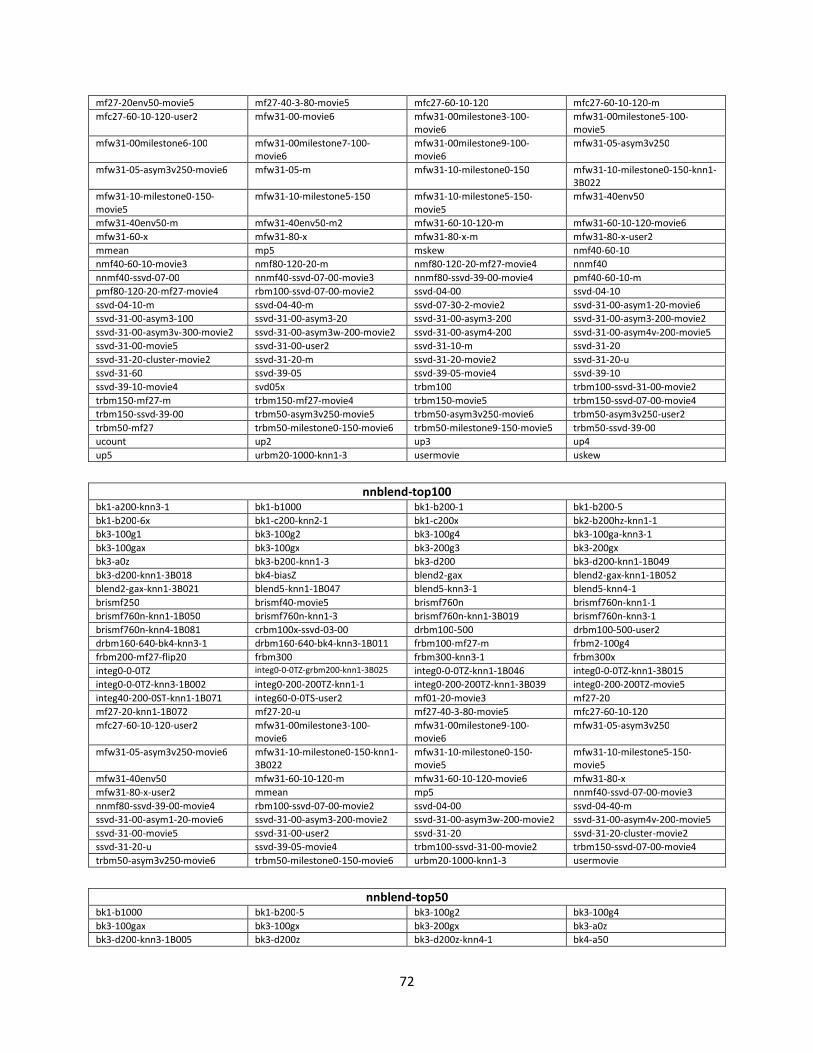
72
mf27-20env50-movie5 mf27-40-3-80-movie5 mfc27-60-10-120 mfc27-60-10-120-m
mfc27-60-10-120-user2 mfw31-00-movie6 mfw31-00milestone3-100-
movie6
mfw31-00milestone5-100-
movie5
mfw31-00milestone6-100 mfw31-00milestone7-100-
movie6
mfw31-00milestone9-100-
movie6
mfw31-05-asym3v250
mfw31-05-asym3v250-movie6 mfw31-05-m mfw31-10-milestone0-150 mfw31-10-milestone0-150-knn1-
3B022
mfw31-10-milestone0-150-
movie5
mfw31-10-milestone5-150 mfw31-10-milestone5-150-
movie5
mfw31-40env50
mfw31-40env50-m mfw31-40env50-m2 mfw31-60-10-120-m mfw31-60-10-120-movie6
mfw31-60-x mfw31-80-x mfw31-80-x-m mfw31-80-x-user2
mmean mp5 mskew nmf40-60-10
nmf40-60-10-movie3 nmf80-120-20-m nmf80-120-20-mf27-movie4 nnmf40
nnmf40-ssvd-07-00 nnmf40-ssvd-07-00-movie3 nnmf80-ssvd-39-00-movie4 pmf40-60-10-m
pmf80-120-20-mf27-movie4 rbm100-ssvd-07-00-movie2 ssvd-04-00 ssvd-04-10
ssvd-04-10-m ssvd-04-40-m ssvd-07-30-2-movie2 ssvd-31-00-asym1-20-movie6
ssvd-31-00-asym3-100 ssvd-31-00-asym3-20 ssvd-31-00-asym3-200 ssvd-31-00-asym3-200-movie2
ssvd-31-00-asym3v-300-movie2 ssvd-31-00-asym3w-200-movie2 ssvd-31-00-asym4-200 ssvd-31-00-asym4v-200-movie5
ssvd-31-00-movie5 ssvd-31-00-user2 ssvd-31-10-m ssvd-31-20
ssvd-31-20-cluster-movie2 ssvd-31-20-m ssvd-31-20-movie2 ssvd-31-20-u
ssvd-31-60 ssvd-39-05 ssvd-39-05-movie4 ssvd-39-10
ssvd-39-10-movie4 svd05x trbm100 trbm100-ssvd-31-00-movie2
trbm150-mf27-m trbm150-mf27-movie4 trbm150-movie5 trbm150-ssvd-07-00-movie4
trbm150-ssvd-39-00 trbm50-asym3v250-movie5 trbm50-asym3v250-movie6 trbm50-asym3v250-user2
trbm50-mf27 trbm50-milestone0-150-movie6 trbm50-milestone9-150-movie5 trbm50-ssvd-39-00
ucount up2 up3 up4
up5 urbm20-1000-knn1-3 usermovie uskew
nnblend-top100
bk1-a200-knn3-1 bk1-b1000 bk1-b200-1 bk1-b200-5
bk1-b200-6x bk1-c200-knn2-1 bk1-c200x bk2-b200hz-knn1-1
bk3-100g1 bk3-100g2 bk3-100g4 bk3-100ga-knn3-1
bk3-100gax bk3-100gx bk3-200g3 bk3-200gx
bk3-a0z bk3-b200-knn1-3 bk3-d200 bk3-d200-knn1-1B049
bk3-d200-knn1-3B018 bk4-biasZ blend2-gax blend2-gax-knn1-1B052
blend2-gax-knn1-3B021 blend5-knn1-1B047 blend5-knn3-1 blend5-knn4-1
brismf250 brismf40-movie5 brismf760n brismf760n-knn1-1
brismf760n-knn1-1B050 brismf760n-knn1-3 brismf760n-knn1-3B019 brismf760n-knn3-1
brismf760n-knn4-1B081 crbm100x-ssvd-03-00 drbm100-500 drbm100-500-user2
drbm160-640-bk4-knn3-1 drbm160-640-bk4-knn3-1B011 frbm100-mf27-m frbm2-100g4
frbm200-mf27-flip20 frbm300 frbm300-knn3-1 frbm300x
integ0-0-0TZ integ0-0-0TZ-grbm200-knn1-3B025 integ0-0-0TZ-knn1-1B046 integ0-0-0TZ-knn1-3B015
integ0-0-0TZ-knn3-1B002 integ0-200-200TZ-knn1-1 integ0-200-200TZ-knn1-3B039 integ0-200-200TZ-movie5
integ40-200-0ST-knn1-1B071 integ60-0-0TS-user2 mf01-20-movie3 mf27-20
mf27-20-knn1-1B072 mf27-20-u mf27-40-3-80-movie5 mfc27-60-10-120
mfc27-60-10-120-user2 mfw31-00milestone3-100-
movie6
mfw31-00milestone9-100-
movie6
mfw31-05-asym3v250
mfw31-05-asym3v250-movie6 mfw31-10-milestone0-150-knn1-
3B022
mfw31-10-milestone0-150-
movie5
mfw31-10-milestone5-150-
movie5
mfw31-40env50 mfw31-60-10-120-m mfw31-60-10-120-movie6 mfw31-80-x
mfw31-80-x-user2 mmean mp5 nnmf40-ssvd-07-00-movie3
nnmf80-ssvd-39-00-movie4 rbm100-ssvd-07-00-movie2 ssvd-04-00 ssvd-04-40-m
ssvd-31-00-asym1-20-movie6 ssvd-31-00-asym3-200-movie2 ssvd-31-00-asym3w-200-movie2 ssvd-31-00-asym4v-200-movie5
ssvd-31-00-movie5 ssvd-31-00-user2 ssvd-31-20 ssvd-31-20-cluster-movie2
ssvd-31-20-u ssvd-39-05-movie4 trbm100-ssvd-31-00-movie2 trbm150-ssvd-07-00-movie4
trbm50-asym3v250-movie6 trbm50-milestone0-150-movie6 urbm20-1000-knn1-3 usermovie
nnblend-top50
bk1-b1000 bk1-b200-5 bk3-100g2 bk3-100g4
bk3-100gax bk3-100gx bk3-200gx bk3-a0z
bk3-d200-knn3-1B005 bk3-d200z bk3-d200z-knn4-1 bk4-a50

73
bk4-b200-knn3-1B101 bk4-biasZ bk5-b200-knn1-1B095 bk5-b200B089
blend2-gax blend2-gax-knn1-1B052 blend5-knn3-1 brismf760n-knn1-1
brismf760n-knn1-1B050 drbm160-640-bk4-knn3-1 drbm160-640-bk4-knn3-1B011 frbm2-100g4
frbm200-mf27-flip20 frbm300 frbm300-knn3-1 frbm300x
integ0-0-0TZ integ0-0-0TZ-grbm200-knn1-
3B025
integ0-0-0TZ-knn1-3B015 integ0-0-0TZ-knn3-1B002
integ0-200-200TZ-knn1-3B039 integ0-200-200TZ-movie5 integ40-200-0ST-knn1-1B071 mf27-20
mf27-20-knn1-1B072 mf27-20-u mfc27-60-10-120 mfw31-05-asym3v250-movie6
mfw31-10-milestone0-150-
movie5
mfw31-10-milestone5-150-
movie5
mfw31-60-10-120-m nnmf80-ssvd-39-00-movie4
ssvd-04-00 ssvd-04-40-m ssvd-31-00-asym1-20-movie6 trbm50-asym3v250-movie6
urbm20-1000-knn1-3 usermovie
nnblend-bottom95
bk1-a200-knn1-1 bk1-a200-knn3-1 bk1-a200x-knn1-1 bk1-a50-2-knn1-1
bk1-b1000 bk1-b200-1 bk1-b200-2 bk1-b200-5x-knn1-3
bk1-b200-6 bk3-100g1 bk3-200g3 bk3-200gx-nlpp1B105
bk3-a50-knn1-3 bk3-c50 bk3-c50x bk4-b200-knn4-1B102
bk5-b200B089-nlpp1B108 blend2-ga1 blend2-ga4 blend2b
blend3-knn2-1 brismf250-movie5 brismf760-movie5 brismf760-user2
brismf760n-knn1-3B019 brismf760n-user2 crbm100 crbm100-ssvd-07-00
crbm200 crbm200-ssvd-07-00 drbm100-500-user2 frbm200-mf27-knn2-2
frbm300-bk4-knn3-1-X-bk3-
b200-knn1-3
frbm300-knn1-1B068 frbm300-movie8 globalEffect14-movie5
gte14b integ0-0-0TZ-flip20-knn2-1 integ0-0-0TZmilestone6-200 integ0-0-0TZmilestone6-200-
knn2-1
integ0-0-0TZmilestone6-200-
movie6
integ0-200-200TZ integ0-200-200TZ-knn1-3 integ0-200-200TZ-knn3-1
integ0-200-200TZ-user2 integ20-100-100NT integ60-0-0TS-movie5 integ80-80-0TZM
integ80-80-0TZM-movie6 mf27-20-movie4 mf27-20-movie5 mf27-20env50-m
mf27-20env50-movie4 mf27-20env50-movie5 mfc27-60-10-120-m mfc27-60-10-120-user2
mfw31-00 mfw31-00-movie6 mfw31-05-asym3v250 mfw31-05-asym3v250-user2
mfw31-10-milestone5-150 mfw31-40env50-m2 mfw31-60-x mfw31-80-x
mskew nmf40-60-10 nmf40-60-10-movie3 nmf80-120-20-m
nmf80-120-20-mf27-movie4 nnmf40-ssvd-07-00 pmf40-60-10-m pmf80-120-20-mf27-movie4
ssvd-04-00 ssvd-07-30-2-movie2 ssvd-31-00-asym3-200 ssvd-31-00-movie
ssvd-31-10-m ssvd-31-20-m ssvd-31-60 ssvd-39-05
ssvd-39-05-movie4 ssvd-39-10 ssvd-39-10-movie4 svd02x
svd05x trbm100-movie2 trbm100-ssvd-31-00 trbm100-ssvd-31-00-movie2
trbm100-ssvd-31-00-user2 trbm150-mf27-movie4 trbm50-asym3v250 trbm50-asym3v250-mfw27-
movie5
trbm50-asym3v250-movie5 trbm50-milestone9-150-movie5 urbm20-1000-knn1-3B020
4.3 Multi-stage blending
Prior to implementing the complete and efficient Neural Network mechanism described above (which
yields better results) we had devised a number of blending techniques to try to capture various aspects
of the data and improve the overall result. These classifiers were used in a stack; each one being trained
on the residual error of the previous with the resulting predictor being the sum of the output of each
classifier. The following subsections describe each classifier (or stage) in this complex blending
mechanism. The final subsection presents the details of the variants that were included in the solution.

74
4.3.1 Multi-linear classifier
This classifier is actually a set of simple linear classifiers trained on a subset of the probe set. The probe
set is divided into n buckets of equal size (number of samples) using user support. The prediction for
each user-movie pair is the output of the linear classifier corresponding to that user’s support.
To refine the training of each classifier, data from neighbouring buckets on both sides is used. If
insufficient buckets are available on one side (for buckets near the start of the end), extra buckets are
taken from the other side to have a constant number of buckets. The samples are given a weight value
which decays linearly with the distance of the sample user’s support to that of the trained bucket
support. This is illustrated in the example chart below, which shows the sample weight per user support
for each bucket. Notice how the bucket starting at 1 has a different weight slope, as all extra buckets are
taken to the right. The number of buckets (N) as well as the width of the base of each bucket (i.e. % of
the total samples used for the training of each bucket) was optimized through validation on the probe
set.
4.3.2 Per-movie Linear classifier
This classifier is another set of simple linear classifiers. This time one classifier is trained for each movie,
using the residual errors from the previous step. First, we compute the regularized mean of each movie
over the probe set as follows:
�� = ∑ �(�)� ∈Ù(�) + ! Ú|¦(�)| + !
Where:
• ¦(�) is the set of ratings for movie m in the probe set;
• �(�) is the rating for item i;
0
0.2
0.4
0.6
0.8
1
1.2
1 11 21 31 41 51 61 71
Sa
mp
le w
eig
ht
User Support

75
• ! is a regularization parameter found through validation on the probe set;
• Ú is the global mean, 3.6043.
Then, the linear equation is solved through Ridge Regression, with each sample being the difference
between the predicted output of the previous stage and ��; optimized towards the difference between
the actual probe rating and ��. Sparseness being an issue, the proper Ridge Regression regularization is
necessary and found manually through validation on the probe set.
4.3.3 Neural-Network classifier
We experimented with using a Neural Network to estimate the residual error after the previous
blending steps. This Neural Network is very similar to the one described in Section 4.2 Neural network
blending, with the following differences:
• Like in [4], a neural network with 12 hidden nodes, and one with 13 hidden nodes are chosen
and then linearly combined;
• The output layer has a linear activation function;
• Weight decay is 0.00012 for both layers;
• Initial learning rate is 0.00012 for both layers;
• Learning rates are decreased linearly to zero over 1000 iterations.
4.3.4 Tree (or GAM) classifier
Prior to implementing the more complex Neural-Network step, we had implemented a Generalized
Additive Model (GAM) classifier to capture non-linearities in the predictor sets. Even after having
implemented the Neural-Network classifier, this classifier still proved useful when trained on the
residual error of that stage.
We define a classifier step function as follows:
�̂(, �) = �$��(, �) + ! l�� �7 I� (, �) < - �� �7 I� (, �) ≥ - < (105)
Where:
• u is the user and m the movie being predicted;
• �$��(, �) is the residual error of the previous classifier for that user-movie pair;
• I� (, �) is the value of predictor � for that user-movie pair;
• �� is the average of all samples in the probe set for which I� < -;
• �� is the average of all samples in the probe set for which I� ≥ -;
• ! is a correction ratio optimized through validation on the probe set.
We find the optimal - and � to minimize the residual error on the probe set. We can generalize this
function to a tree function with two levels:

76
�̂(, �) = �$��(, �) + ! ./0/1Û�� �7 I� (, �) < - ��E Id (, �) < b�� �7 I� (, �) < - ��E Id (, �) ≥ b<
l�� �7 I� (, �) ≥ - ��E I\ (, �) < ^�&�7 I� (, �) ≥ - ��E I\ (, �) ≥ ^< < (106)
Where:
• I� (, �), Id (, �) and I\(, �) are the values of predictors �, c ��E Z for that user-movie pair;
• �� is the average of all samples in the probe set for which I� < - ��E Id < b;
• �� is the average of all samples in the probe set for which I� < - ��E Id ≥ b;
• �� is the average of all samples in the probe set for which I� ≥ - ��E I\ < ^;
• �& is the average of all samples in the probe set for which I� ≥ - ��E I\ ≥ ^;
Because of processing issues, we first find - and � as in the step function above. Then, we find b, ^, c and Z to minimize the residual error on the probe set.
Finally, we define the GAM classifier as a stacking of n of these tree functions trained on the residual
error of the previous ones. The value of n is optimized through validation on the probe set. Note that to
avoid overfitting, the number of samples which fall in a particular quadrant is limited to a minimum
value and the correction in each tree function limited by multiplying the output by a certain ratio. Each
of these meta-parameters was optimized manually through validation on the probe set.
4.3.5 Clipping
The final step in our multi-stage classifier is the clipping stage. The minimum threshold X��� is chosen as
the highest value for which the predicted output is lower than the average of the probe set scores that
have a predicted output below X���. All values below that threshold are clamped to X���. The maximum
clamping threshold X��, is found similarly.
4.3.6 Variants
Two predictors produced with this multi-stage blending approach were included in the solution. The
following tables indicate the parameters used in these blends. Note that the Neural-Network
parameters are described in the corresponding section above.
Variant Multi-Linear Movie-Linear Neural-Network
Used? N Base offset slope !
pragmatictheory-20090316 50 50% 1200 350 1 Y
pragmatictheory-20090527 50 50% 1200 350 1 N
Variant Tree Clipping Number of sets
nb tree min samples corr. ratio X��� X��,
pragmatictheory-20090316 221 5000 0.10 1.0398 4.9616 233
pragmatictheory-20090527 142 5000 0.25 1.0599 4.9659 208
The following tables show the list of predictors used in each case:

77
pragmatictheory-20090316
bk1-a1000x brismf760n-knn1-1 integ80-80-0TZM ssvd-31-00-asym1-20-movie6
bk1-a1000x-knn1-3 brismf760n-knn1-3 integ80-80-0TZM-movie6 ssvd-31-00-asym3-100
bk1-a200-knn1-1 brismf760n-knn3-1 integ80-80-0TZ-movie5 ssvd-31-00-asym3-20
bk1-a200-knn1-3 brismf760n-movie5 mf01-20-movie3 ssvd-31-00-asym3-200
bk1-a200-knn3-1 brismf760n-movie6 mf01-40-3-80-movie4 ssvd-31-00-asym3-200-movie2
bk1-a200x-knn1-1 brismf760n-user2 mf27-20 ssvd-31-00-asym3v-300-movie2
bk1-a50 brismf760-user2 mf27-20env50-m ssvd-31-00-asym3w-200-movie2
bk1-a50-2 crbm100 mf27-20env50-movie4 ssvd-31-00-asym4-200
bk1-a50-2-knn1-1 crbm100-movie2 mf27-20env50-movie5 ssvd-31-00-asym4v-200-movie5
bk1-a50-2x crbm100-ssvd-07-00 mf27-20-movie4 ssvd-31-00-movie
bk1-a50-movie5 crbm100-ssvd-07-00-movie2 mf27-20-movie5 ssvd-31-00-movie5
bk1-b1000 crbm100-ssvd-07-20 mf27-20-u ssvd-31-10-m
bk1-b200-1 crbm100x-ssvd-03-00 mf27-40-3-80-movie5 ssvd-31-20
bk1-b200-1-knn1-0 crbm200 mfc27-60-10-120 ssvd-31-20-cluster-movie2
bk1-b200-1-knn1-1 crbm200-ssvd-07-00 mfc27-60-10-120-m ssvd-31-20-m
bk1-b200-2 drbm100-500 mfc27-60-10-120-user2 ssvd-31-20-movie2
bk1-b200-5 drbm100-500-mfw31-m mfw31-00 ssvd-31-20-u
bk1-b200-5x drbm100-500-user2
mfw31-00milestone3-100-
movie6 ssvd-31-60
bk1-b200-5x-knn1-3 drbm160-640
mfw31-00milestone4-100-
movie5 ssvd-39-05
bk1-b200-6 drbm160-640-knn3-1
mfw31-00milestone5-100-
movie5 ssvd-39-05-movie4
bk1-b200-6x drbm160-640-knn4-1 mfw31-00milestone6-100 ssvd-39-10
bk1-c200-knn2-1 frbm100-mf27-m
mfw31-00milestone7-100-
movie6 ssvd-39-10-movie4
bk1-c200x frbm200
mfw31-00milestone9-100-
movie6 ssvd-63-00
bk2-b200hz-knn1-1 frbm200-mf27-flip20 mfw31-00-movie6 ssvd-63-00-movie4
bk3-100g1 frbm200-mf27-knn2-2 mfw31-05-asym3v250 ssvd-63-30
bk3-100g2 frbm200x mfw31-05-asym3v250-movie6 ssvd-63-30-movie4
bk3-100g4 frbm2-100g3 mfw31-05-asym3v250-user2 svd02x
bk3-100ga1 frbm2-100g4 mfw31-05-m svd05x
bk3-100ga4 frbm2-100gx-knn2-1 mfw31-10-milestone0-150 trbm100
bk3-100ga-knn3-1 frbm300
mfw31-10-milestone0-150-
movie5 trbm100-movie2
bk3-100gax frbm300-knn3-1 mfw31-10-milestone5-150 trbm100-ssvd-31-00
bk3-100gx frbm300-movie8
mfw31-10-milestone5-150-
movie5 trbm100-ssvd-31-00-movie2
bk3-200g1 frbm300x mfw31-40env50 trbm100-ssvd-31-00-user2
bk3-200g3 globalEffect14-movie5 mfw31-40env50-m trbm150-mf27-m
bk3-200g4 gte14b mfw31-40env50-m2 trbm150-mf27-movie4
bk3-200g-knn2-1 integ0-0-0TZ mfw31-60-10-120-m trbm150-movie5
bk3-200gx integ0-0-0TZ-flip20-knn2-1 mfw31-60-10-120-movie6 trbm150-ssvd-07-00-movie4
bk3-a50-knn1-3 integ0-0-0TZ-grbm200 mfw31-60-x trbm150-ssvd-39-00
bk3-b200-knn1-3 integ0-0-0TZmilestone6-200 mfw31-80-x trbm50-asym3v250
bk3-c50
integ0-0-0TZmilestone6-200-
knn2-1 mfw31-80-x-m
trbm50-asym3v250-mfw27-
movie5
bk3-c50-knn2-1
integ0-0-0TZmilestone6-200-
movie6 mfw31-80-x-user2 trbm50-asym3v250-movie5
bk3-c50-knn3-1 integ0-0-0TZ-movie6 mmean trbm50-asym3v250-movie6
bk3-c50x integ0-100-100TZ mp5 trbm50-asym3v250-user2
bk3-d200 integ0-100-100TZ-movie6 mskew trbm50-mf27
bk3-d200z integ0-200-200NT nmf40-60-10 trbm50-milestone0-150-movie6
bk3-d200z-knn4-1 integ0-200-200NT-user2 nmf40-60-10-movie3 trbm50-milestone9-150-movie5
blend2b integ0-200-200TZ nmf80-120-20-m trbm50-ssvd-39-00
blend2-ga1 integ0-200-200TZ-knn1-1 nmf80-120-20-mf27-movie4 ucount
blend2-ga4 integ0-200-200TZ-knn1-3 nnmf40 up2
blend2-ga-knn2-1 integ0-200-200TZ-knn2-1 nnmf40-ssvd-07-00 up3
blend2-gax integ0-200-200TZ-knn3-1 nnmf40-ssvd-07-00-movie3 up4
blend3-knn2-1 integ0-200-200TZ-movie5 nnmf80-ssvd-39-00-movie4 up5
blend5-knn3-1 integ0-200-200TZ-user2 pmf40-60-10-m urbm20-1000

78
blend5-knn4-1 integ20-100-100NT pmf80-120-20-mf27-movie4 urbm20-1000-knn1-3
brismf250 integ40-200-0ST rbm100-ssvd-07-00-movie2 usermovie
brismf250-movie5 integ40-200-0T ssvd-04-00 uskew
brismf40-movie5 integ60-0-0TS ssvd-04-10-m
brismf760-movie5 integ60-0-0TS-movie5 ssvd-04-40-m
brismf760n integ60-0-0TS-user2 ssvd-07-30-2-movie2
pragmatictheory-20090527
bk1-a200-knn3-1 brismf760n-knn1-3B019 integ60-0-0TS-user2 nnmf80-ssvd-39-00-movie4
bk1-a200x-knn1-1 brismf760n-knn3-1 integ80-80-0TZ-movie5 pmf40-60-10-m
bk1-a50 brismf760n-knn4-1B081 integ80-80-0TZM pmf80-120-20-mf27-movie4
bk1-a50-2-knn1-1 brismf760n-user2 integ80-80-0TZM-movie6 rbm100-ssvd-07-00-movie2
bk1-a50-2x crbm100 mf01-20-movie3 ssvd-04-00
bk1-a50-movie5 crbm100-movie2 mf01-40-3-80-movie4 ssvd-04-10-m
bk1-b1000 crbm100-ssvd-07-00 mf27-20 ssvd-04-40-m
bk1-b200-1 crbm100-ssvd-07-00-movie2 mf27-20-knn1-1B072 ssvd-07-30-2-movie2
bk1-b200-1-knn1-0 crbm100-ssvd-07-20 mf27-20-movie4 ssvd-31-00-asym1-20-movie6
bk1-b200-1-knn1-1 crbm100x-ssvd-03-00 mf27-20-movie5 ssvd-31-00-asym3-100
bk1-b200-2 crbm200-ssvd-07-00 mf27-20-u ssvd-31-00-asym3-20
bk1-b200-5 drbm100-500 mf27-20env50-m ssvd-31-00-asym3-200
bk1-b200-6x drbm100-500-user2 mf27-20env50-movie4 ssvd-31-00-asym3-200-movie2
bk1-c200-knn2-1 drbm160-640 mf27-20env50-movie5 ssvd-31-00-asym3v-300-movie2
bk1-c200x drbm160-640-bk4-knn3-1 mf27-40-3-80-movie5 ssvd-31-00-asym3w-200-movie2
bk2-b200hz-knn1-1 drbm160-640-bk4-knn3-1B011 mfc27-60-10-120 ssvd-31-00-asym4-200
bk3-100g1 drbm160-640-knn3-1 mfc27-60-10-120-m ssvd-31-00-asym4v-200-movie5
bk3-100g2 drbm160-640-knn4-1 mfc27-60-10-120-user2 ssvd-31-00-movie
bk3-100g4 frbm100-mf27-m mfw31-00 ssvd-31-00-movie5
bk3-100ga-knn3-1 frbm2-100g3 mfw31-00-movie6 ssvd-31-10-m
bk3-100ga4 frbm2-100g4
mfw31-00milestone3-100-
movie6 ssvd-31-20
bk3-100gax frbm200
mfw31-00milestone4-100-
movie5 ssvd-31-20-cluster-movie2
bk3-100gx frbm200-mf27-flip20
mfw31-00milestone5-100-
movie5 ssvd-31-20-m
bk3-200g1 frbm200-mf27-knn2-2 mfw31-00milestone6-100 ssvd-31-20-movie2
bk3-200g3 frbm200x
mfw31-00milestone7-100-
movie6 ssvd-31-20-u
bk3-200g4 frbm300
mfw31-00milestone9-100-
movie6 ssvd-31-60
bk3-200gx frbm300-bk4-knn3-1 mfw31-05-asym3v250 ssvd-39-05
bk3-a50-knn1-3 frbm300-knn1-1B068 mfw31-05-asym3v250-movie6 ssvd-39-05-movie4
bk3-b200-knn1-3 frbm300-knn3-1 mfw31-05-asym3v250-user2 ssvd-39-10
bk3-c50 frbm300x mfw31-05-m ssvd-39-10-movie4
bk3-c50-knn2-1 integ0-0-0TZ mfw31-10-milestone0-150 svd05x
bk3-d200 integ0-0-0TZ-flip20-knn2-1
mfw31-10-milestone0-150-knn1-
3B022 trbm100
bk3-d200z
integ0-0-0TZ-grbm200-knn1-
3B025
mfw31-10-milestone0-150-
movie5 trbm100-ssvd-31-00-movie2
bk3-d200z-knn4-1 integ0-0-0TZ-knn1-1B046 mfw31-10-milestone5-150 trbm150-mf27-m
bk4-biasZ integ0-0-0TZ-knn1-3B015
mfw31-10-milestone5-150-
movie5 trbm150-mf27-movie4
blend2-ga-knn2-1 integ0-0-0TZ-knn3-1B002 mfw31-40env50 trbm150-ssvd-07-00-movie4
blend2-ga1 integ0-0-0TZ-movie6 mfw31-60-10-120-m trbm150-ssvd-39-00
blend2-ga4 integ0-0-0TZmilestone6-200 mfw31-60-10-120-movie6 trbm50-asym3v250-movie5
blend2-gax
integ0-0-0TZmilestone6-200-
movie6 mfw31-60-x trbm50-asym3v250-movie6
blend2-gax-knn1-1B052 integ0-100-100TZ mfw31-80-x trbm50-asym3v250-user2
blend2b integ0-100-100TZ-movie6 mfw31-80-x-m trbm50-mf27
blend5-knn1-1B047 integ0-200-200NT mfw31-80-x-user2 trbm50-milestone0-150-movie6
blend5-knn3-1 integ0-200-200NT-user2 mmean trbm50-milestone9-150-movie5
blend5-knn4-1 integ0-200-200TZ mp5 trbm50-ssvd-39-00
brismf250 integ0-200-200TZ-knn1-1 mskew ucount

79
brismf250-movie5 integ0-200-200TZ-knn3-1 nmf40-60-10 up2
brismf40-movie5 integ0-200-200TZ-user2 nmf40-60-10-movie3 up3
brismf760-movie5 integ20-100-100NT nmf80-120-20-m up4
brismf760n integ40-200-0ST nmf80-120-20-mf27-movie4 up5
brismf760n-knn1-1 integ40-200-0T nnmf40 urbm20-1000-knn1-3
brismf760n-knn1-1B050 integ60-0-0TS nnmf40-ssvd-07-00 usermovie
brismf760n-knn1-3 integ60-0-0TS-movie5 nnmf40-ssvd-07-00-movie3 uskew
4.4 Variable multiplications
In the late stages of the competition, we used a final blending step consisting of a linear regression
blending done directly on quiz sets, as described in [7]. Since this type of blending is linear in nature, it
can only capture certain relationships between predictors. In order to try to capture non-linear aspects,
we introduced new predictors which consist of simple arithmetic multiplications of pairs of base
predictors. This technique is suggested in [6].
In order to find the best pairs of predictors to multiply, we constructed a baseline using a linear
regression of the 233 sets in the pragmatictheory-20090316 blend. Then, we added, in turn, each
possible pair of predictors multiplied together and compute the linear blend again. Finally, the pair
which improves the blend result the most is selected. This new predictor is added to the baseline and
the algorithm is run again. This method is known as forward selection. The following table presents the
predictors that were introduced to the solution using this technique.
Name Base predictor 1 Base predictor 2
bk3-200g3-X-bk3-100ga4 bk3-200g3 bk3-100ga4
nnmf80-ssvd-39-00-movie4-X-blend2-ga4 nnmf80-ssvd-39-00-movie4 blend2-ga4
ucount-X-drbm100-500 ucount drbm100-500
ucount-X-nmf80-120-20-m ucount nmf80-120-20-m
frbm300-bk4-knn3-1-X-bk3-b200-knn1-3 frbm300-bk4-knn3-1 bk3-b200-knn1-3

80
5 Towards a better recommendation system The solution presented in this document was exclusively aimed at building a system that would predict
subscriber ratings with the highest possible accuracy. Although highly accurate predictions are an
important part of a recommender system, these alone cannot ensure good recommendations.
Moreover, the solution is based on a huge amount of models and predictors which would not be
practical as part of a commercial recommender system. However, this result is a direct consequence of
the nature and goal of the competition: obtain the highest possible accuracy at any cost, disregarding
completely the complexity of the solution and the execution performance.
On the other hand, we believe that a real life recommender system can benefit from some of the
techniques and algorithms proposed in this document. In our opinion, the following are our most
worthwhile innovations:
• The use of the frequency measure leads to higher accuracy. Frequency was most useful for
movie related coefficients. This variable is especially useful because it can be used even with
new customers that have a short history of ratings.
• The classification view of linear models using logistic transformation allows for increased blend
accuracy, using the same basic algorithm.
• The non-linear envelope allows greater model accuracy with virtually no increase in model
complexity.
• We presented an extension to Koren's integrated model that achieves very high accuracy (bk4-
f200z4-nlpp1-knn3-1 has a quiz RMSE of 0.8713). One innovative contribution is to use a low
rank matrix factorization to capture time-dependent biases.
• We also presented an extension to Bell and Koren's neighbourhood approach that has been
successful at improving virtually any model (kNN3). One innovative contribution was to
estimate neighbour weights by combining the residual error and a simple baseline.
• We demonstrated the use of automatic parameter tuning across multiple model types using the
Nelder-Mead Simplex Method, which greatly reduces the manual effort required to adjust
model meta-parameters.
We believe the methods presented here will allow the creation of higher accuracy recommendation
systems or, at the very least, simpler ones with equivalent accuracy. For example, the 2007 Progress
Prize was won with an entry consisting of 107 predictors with a quiz set accuracy of 0.8712. Currently,
we can achieve accuracy within 0.0001 of this milestone using a single predictor (bk4-f200z4-nlpp1-
knn3-1). This illustrates the progress made in collaborative filtering algorithms over the past two years.

81
6 Acknowledgments We would like to take this opportunity to acknowledge all the people who assisted us throughout the
competition.
First, special thanks are given to Yehuda Koren for his numerous publications that have been an
inspiration to us and for his insightful comments.
We also thank Andreas Töscher and Michael Jahrer for their help with Neural Network blending and for
their suggestion to optimize model parameters directly on the blended score.
We would also like to express our gratitude to all the teams and individuals who offered their assistance
throughout the competition, especially during the hectic last day. In addition, acknowledgments go out
to everyone who shared insight through publications, blogs or the Netflix Prize forum during the course
of the competition.
Finally, we would like to extend our sincere thanks to Netflix who had the vision and courage to harness
the power of the community.

82
7 List of predictors
The following table lists all predictors that were included in the final quiz blend, sorted alphabetically.
Name Probe RMSE Quiz RMSE
bk1-a1000-nlpp1B107 0.8891 0.8815
bk1-a1000x 0.8876 0.8794
bk1-a1000x-knn1-3 0.8855 0.8766
bk1-a1000x-knn1-5B131 0.8888 0.8803
bk1-a200-knn1-1 0.8873 0.8787
bk1-a200-knn1-3 0.8865 0.8776
bk1-a200-knn3-1 0.8847 0.8762
bk1-a200x-knn1-1 0.8861 0.8773
bk1-a50 0.8917 0.8844
bk1-a50-2 0.8917 0.8844
bk1-a50-2-knn1-1 0.8889 0.8803
bk1-a50-2x 0.8898 0.8819
bk1-a50-movie5 0.8887 0.8797
bk1-b1000 0.8863 0.8781
bk1-b200-1 0.8877 0.8792
bk1-b200-1-knn1-0 0.8872 0.8777
bk1-b200-1-knn1-1 0.8871 0.8776
bk1-b200-2 0.8880 0.8795
bk1-b200-5 0.8872 0.8789
bk1-b200-5-knn1-1B060 0.8868 0.8777
bk1-b200-5x 0.8865 0.8778
bk1-b200-5x-knn1-3 0.8858 0.8766
bk1-b200-6 0.8865 0.8784
bk1-b200-6x 0.8854 0.8768
bk1-c200-knn2-1 0.8840 0.8755
bk1-c200x 0.8855 0.8770
bk2-b200h 0.8868 0.8785
bk2-b200hz-knn1-1 0.8851 0.8761
bk3-100g1 1.0426 1.0411
bk3-100g2 0.9725 0.9698
bk3-100g4 0.9717 0.9684
bk3-100ga1 1.0411 1.0395
bk3-100ga4 0.9697 0.9663
bk3-100ga-knn3-1 0.8821 0.8747
bk3-100gax 0.8879 0.8818
bk3-100gx 0.8895 0.8836
bk3-200g1 1.0385 1.0366
bk3-200g3 0.9140 0.9092
bk3-200g3-X-bk3-100ga4 0.9616 0.9577
bk3-200g4 0.9669 0.9631
bk3-200g-knn2-1 0.8812 0.8738
bk3-200gx 0.8851 0.8785
bk3-a0z 0.9610 0.9555
bk3-a50-knn1-3 0.8901 0.8817
bk3-b200-knn1-3 0.8901 0.8814
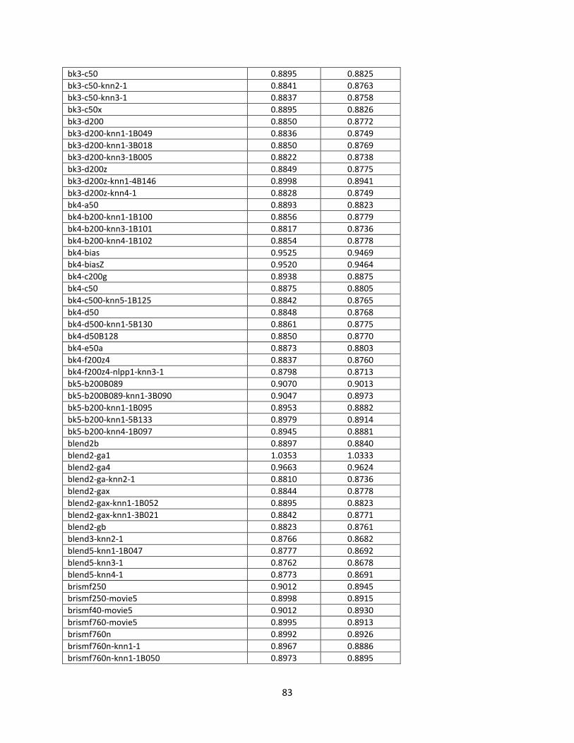
83
bk3-c50 0.8895 0.8825
bk3-c50-knn2-1 0.8841 0.8763
bk3-c50-knn3-1 0.8837 0.8758
bk3-c50x 0.8895 0.8826
bk3-d200 0.8850 0.8772
bk3-d200-knn1-1B049 0.8836 0.8749
bk3-d200-knn1-3B018 0.8850 0.8769
bk3-d200-knn3-1B005 0.8822 0.8738
bk3-d200z 0.8849 0.8775
bk3-d200z-knn1-4B146 0.8998 0.8941
bk3-d200z-knn4-1 0.8828 0.8749
bk4-a50 0.8893 0.8823
bk4-b200-knn1-1B100 0.8856 0.8779
bk4-b200-knn3-1B101 0.8817 0.8736
bk4-b200-knn4-1B102 0.8854 0.8778
bk4-bias 0.9525 0.9469
bk4-biasZ 0.9520 0.9464
bk4-c200g 0.8938 0.8875
bk4-c50 0.8875 0.8805
bk4-c500-knn5-1B125 0.8842 0.8765
bk4-d50 0.8848 0.8768
bk4-d500-knn1-5B130 0.8861 0.8775
bk4-d50B128 0.8850 0.8770
bk4-e50a 0.8873 0.8803
bk4-f200z4 0.8837 0.8760
bk4-f200z4-nlpp1-knn3-1 0.8798 0.8713
bk5-b200B089 0.9070 0.9013
bk5-b200B089-knn1-3B090 0.9047 0.8973
bk5-b200-knn1-1B095 0.8953 0.8882
bk5-b200-knn1-5B133 0.8979 0.8914
bk5-b200-knn4-1B097 0.8945 0.8881
blend2b 0.8897 0.8840
blend2-ga1 1.0353 1.0333
blend2-ga4 0.9663 0.9624
blend2-ga-knn2-1 0.8810 0.8736
blend2-gax 0.8844 0.8778
blend2-gax-knn1-1B052 0.8895 0.8823
blend2-gax-knn1-3B021 0.8842 0.8771
blend2-gb 0.8823 0.8761
blend3-knn2-1 0.8766 0.8682
blend5-knn1-1B047 0.8777 0.8692
blend5-knn3-1 0.8762 0.8678
blend5-knn4-1 0.8773 0.8691
brismf250 0.9012 0.8945
brismf250-movie5 0.8998 0.8915
brismf40-movie5 0.9012 0.8930
brismf760-movie5 0.8995 0.8913
brismf760n 0.8992 0.8926
brismf760n-knn1-1 0.8967 0.8886
brismf760n-knn1-1B050 0.8973 0.8895
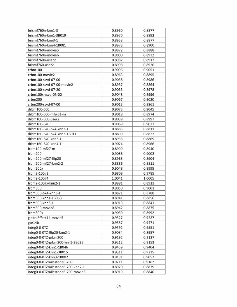
84
brismf760n-knn1-3 0.8960 0.8877
brismf760n-knn1-3B019 0.8970 0.8892
brismf760n-knn3-1 0.8953 0.8877
brismf760n-knn4-1B081 0.8973 0.8900
brismf760n-movie5 0.8972 0.8888
brismf760n-movie6 0.9000 0.8932
brismf760n-user2 0.8987 0.8917
brismf760-user2 0.8998 0.8926
crbm100 0.9096 0.9051
crbm100-movie2 0.8963 0.8895
crbm100-ssvd-07-00 0.9038 0.8986
crbm100-ssvd-07-00-movie2 0.8937 0.8864
crbm100-ssvd-07-20 0.9033 0.8978
crbm100x-ssvd-03-00 0.9048 0.8996
crbm200 0.9067 0.9020
crbm200-ssvd-07-00 0.9013 0.8961
drbm100-500 0.9073 0.9045
drbm100-500-mfw31-m 0.9018 0.8974
drbm100-500-user2 0.9039 0.8997
drbm160-640 0.9069 0.9027
drbm160-640-bk4-knn3-1 0.8885 0.8811
drbm160-640-bk4-knn3-1B011 0.8899 0.8822
drbm160-640-knn3-1 0.8936 0.8869
drbm160-640-knn4-1 0.9024 0.8966
frbm100-mf27-m 0.8999 0.8940
frbm200 0.9056 0.9002
frbm200-mf27-flip20 0.8965 0.8904
frbm200-mf27-knn2-2 0.8886 0.8811
frbm200x 0.9048 0.8995
frbm2-100g3 0.9809 0.9785
frbm2-100g4 1.0041 1.0005
frbm2-100gx-knn2-1 0.8991 0.8911
frbm300 0.9050 0.9001
frbm300-bk4-knn3-1 0.8871 0.8788
frbm300-knn1-1B068 0.8941 0.8856
frbm300-knn3-1 0.8913 0.8841
frbm300-movie8 0.8942 0.8875
frbm300x 0.9039 0.8992
globalEffect14-movie5 0.9327 0.9227
gte14b 0.9537 0.9471
integ0-0-0TZ 0.9592 0.9551
integ0-0-0TZ-flip20-knn2-1 0.9034 0.8957
integ0-0-0TZ-grbm200 0.9192 0.9137
integ0-0-0TZ-grbm200-knn1-3B025 0.9212 0.9153
integ0-0-0TZ-knn1-1B046 0.9459 0.9404
integ0-0-0TZ-knn1-3B015 0.9311 0.9235
integ0-0-0TZ-knn3-1B002 0.9131 0.9052
integ0-0-0TZmilestone6-200 0.9211 0.9162
integ0-0-0TZmilestone6-200-knn2-1 0.8920 0.8839
integ0-0-0TZmilestone6-200-movie6 0.8919 0.8840

85
integ0-0-0TZ-movie6 0.9079 0.9003
integ0-100-100TZ 0.8981 0.8921
integ0-100-100TZ-movie6 0.8911 0.8837
integ0-200-200NT 0.9057 0.8996
integ0-200-200NT-user2 0.9037 0.8972
integ0-200-200TZ 0.8969 0.8906
integ0-200-200TZ-knn1-1 0.8931 0.8845
integ0-200-200TZ-knn1-3 0.8924 0.8836
integ0-200-200TZ-knn1-3B039 0.8949 0.8869
integ0-200-200TZ-knn2-1 0.8891 0.8814
integ0-200-200TZ-knn3-1 0.8889 0.8811
integ0-200-200TZ-movie5 0.8920 0.8829
integ0-200-200TZ-user2 0.8963 0.8895
integ20-100-100NT 0.9003 0.8946
integ40-200-0ST 0.8995 0.8939
integ40-200-0ST-knn1-1B071 0.8982 0.8914
integ40-200-0T 0.8999 0.8936
integ60-0-0TS 0.9048 0.8988
integ60-0-0TS-movie5 0.8998 0.8912
integ60-0-0TS-user2 0.9014 0.8948
integ80-80-0TZM 0.8989 0.8927
integ80-80-0TZM-movie6 0.8909 0.8831
integ80-80-0TZ-movie5 0.8907 0.8817
mf01-20-movie3 0.9038 0.8974
mf01-40-3-80-movie4 0.9044 0.8984
mf27-20 0.9078 0.9020
mf27-20env50-m 0.8984 0.8915
mf27-20env50-movie4 0.8988 0.8919
mf27-20env50-movie5 0.8985 0.8904
mf27-20-knn1-1B072 0.9064 0.8993
mf27-20-movie4 0.8995 0.8922
mf27-20-movie5 0.9005 0.8917
mf27-20-u 0.9071 0.9014
mf27-40-3-80-movie5 0.8990 0.8900
mfc27-60-10-120 0.9072 0.9017
mfc27-60-10-120-m 0.8996 0.8918
mfc27-60-10-120-user2 0.9051 0.8991
mfw31-00 0.9708 0.9665
mfw31-00milestone3-100-movie6 0.8961 0.8876
mfw31-00milestone4-100-movie5 0.9036 0.8935
mfw31-00milestone5-100-movie5 0.9031 0.8932
mfw31-00milestone6-100 0.9289 0.9235
mfw31-00milestone7-100-movie6 0.8954 0.8869
mfw31-00milestone9-100-movie6 0.8954 0.8869
mfw31-00-movie6 0.9124 0.9040
mfw31-05-asym3v250 0.9083 0.9024
mfw31-05-asym3v250-movie6 0.8919 0.8838
mfw31-05-asym3v250-user2 0.9031 0.8963
mfw31-05-m 0.9176 0.9091
mfw31-10-milestone0-150 0.9055 0.8994

86
mfw31-10-milestone0-150-knn1-3B022 0.9049 0.8977
mfw31-10-milestone0-150-movie5 0.8972 0.8874
mfw31-10-milestone5-150 0.9049 0.8989
mfw31-10-milestone5-150-movie5 0.8966 0.8869
mfw31-40env50 0.9017 0.8966
mfw31-40env50-m 0.8961 0.8887
mfw31-40env50-m2 0.8948 0.8874
mfw31-60-10-120-m 0.8965 0.8883
mfw31-60-10-120-movie6 0.8978 0.8906
mfw31-60-x 0.9027 0.8968
mfw31-80-x 0.9031 0.8973
mfw31-80-x-m 0.8965 0.8890
mfw31-80-x-user2 0.9012 0.8948
mmean 1.0516 1.0520
mp5 1.0648 1.0657
mskew 1.0687 1.0691
nmf40-60-10 0.9138 0.9089
nmf40-60-10-movie3 0.9068 0.9005
nmf80-120-20-m 0.9069 0.8997
nmf80-120-20-mf27-movie4 0.9012 0.8942
nnmf40 0.9156 0.9088
nnmf40-ssvd-07-00 0.9122 0.9050
nnmf40-ssvd-07-00-movie3 0.9056 0.8971
nnmf80-ssvd-39-00-movie4 0.9019 0.8933
nnmf80-ssvd-39-00-movie4-X-blend2-ga4 0.9639 0.9597
pmf40-60-10-m 0.9102 0.9033
pmf80-120-20-mf27-movie4 0.9024 0.8957
rbm100-ssvd-07-00-movie2 0.8949 0.8878
ssvd-04-00 0.9891 0.9872
ssvd-04-10 0.9278 0.9236
ssvd-04-10-m 0.9160 0.9099
ssvd-04-40-m 0.9136 0.9073
ssvd-07-30-2-movie2 0.9263 0.9197
ssvd-31-00-asym1-20-movie6 0.9063 0.8987
ssvd-31-00-asym3-100 0.9279 0.9227
ssvd-31-00-asym3-20 0.9311 0.9262
ssvd-31-00-asym3-200 0.9275 0.9223
ssvd-31-00-asym3-200-movie2 0.8990 0.8909
ssvd-31-00-asym3v-300-movie2 0.8984 0.8902
ssvd-31-00-asym3w-200-movie2 0.8986 0.8905
ssvd-31-00-asym4-200 0.9254 0.9201
ssvd-31-00-asym4v-200-movie5 0.9055 0.8959
ssvd-31-00-movie 0.9166 0.9091
ssvd-31-00-movie5 0.9323 0.9234
ssvd-31-00-user2 0.9290 0.9230
ssvd-31-10-m 0.9124 0.9049
ssvd-31-20 0.9185 0.9124
ssvd-31-20-cluster-movie2 0.9047 0.8971
ssvd-31-20-m 0.9100 0.9020
ssvd-31-20-movie2 0.9059 0.8982

87
ssvd-31-20-u 0.9172 0.9112
ssvd-31-60 0.9165 0.9102
ssvd-39-05 0.9282 0.9239
ssvd-39-05-movie4 0.9061 0.8991
ssvd-39-10 0.9215 0.9169
ssvd-39-10-movie4 0.9053 0.8985
ssvd-63-00 0.9593 0.9545
ssvd-63-00-movie4 0.9138 0.9058
ssvd-63-30 0.9148 0.9086
ssvd-63-30-movie4 0.9046 0.8971
svd02x 0.9496 0.9461
svd05x 0.9376 0.9336
trbm100 0.9087 0.9036
trbm100-movie2 0.8956 0.8884
trbm100-ssvd-31-00 0.9043 0.8989
trbm100-ssvd-31-00-movie2 0.8948 0.8874
trbm100-ssvd-31-00-user2 0.9017 0.8955
trbm150-mf27-m 0.8986 0.8926
trbm150-mf27-movie4 0.8921 0.8849
trbm150-movie5 0.8944 0.8860
trbm150-ssvd-07-00-movie4 0.8939 0.8869
trbm150-ssvd-39-00 0.9003 0.8946
trbm50-asym3v250 0.9112 0.9072
trbm50-asym3v250-mfw27-movie5 0.8931 0.8845
trbm50-asym3v250-movie5 0.8957 0.8872
trbm50-asym3v250-movie6 0.8929 0.8863
trbm50-asym3v250-user2 0.9073 0.9021
trbm50-mf27 0.9077 0.9026
trbm50-milestone0-150-movie6 0.8936 0.8869
trbm50-milestone9-150-movie5 0.8955 0.8871
trbm50-ssvd-39-00 0.9079 0.9030
ucount 1.1264 1.1277
ucount-X-drbm100-500 1.1266 1.1279
ucount-X-nmf80-120-20-m 1.1264 1.1276
up2 1.0947 1.0936
up3 1.1004 1.1001
up4 1.1271 1.1285
up5 1.0813 1.0799
urbm20-1000 0.9366 0.9311
urbm20-1000-knn1-3 0.9253 0.9167
usermovie 0.9823 0.9802
uskew 1.1059 1.1050
The following table lists additional predictors that were not included as part of the final quiz blend, but
were included in the solution through probe-based blending. The quiz RMSE for these predictors is not
available.
Name Probe RMSE
bk1-a1000x-knn1-4B145 0.8875
bk1-a1000x-knn5-8B111 0.8865
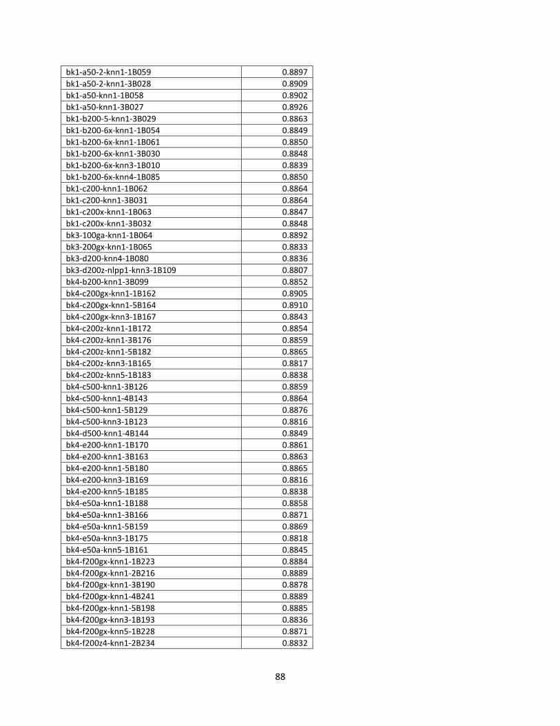
88
bk1-a50-2-knn1-1B059 0.8897
bk1-a50-2-knn1-3B028 0.8909
bk1-a50-knn1-1B058 0.8902
bk1-a50-knn1-3B027 0.8926
bk1-b200-5-knn1-3B029 0.8863
bk1-b200-6x-knn1-1B054 0.8849
bk1-b200-6x-knn1-1B061 0.8850
bk1-b200-6x-knn1-3B030 0.8848
bk1-b200-6x-knn3-1B010 0.8839
bk1-b200-6x-knn4-1B085 0.8850
bk1-c200-knn1-1B062 0.8864
bk1-c200-knn1-3B031 0.8864
bk1-c200x-knn1-1B063 0.8847
bk1-c200x-knn1-3B032 0.8848
bk3-100ga-knn1-1B064 0.8892
bk3-200gx-knn1-1B065 0.8833
bk3-d200-knn4-1B080 0.8836
bk3-d200z-nlpp1-knn3-1B109 0.8807
bk4-b200-knn1-3B099 0.8852
bk4-c200gx-knn1-1B162 0.8905
bk4-c200gx-knn1-5B164 0.8910
bk4-c200gx-knn3-1B167 0.8843
bk4-c200z-knn1-1B172 0.8854
bk4-c200z-knn1-3B176 0.8859
bk4-c200z-knn1-5B182 0.8865
bk4-c200z-knn3-1B165 0.8817
bk4-c200z-knn5-1B183 0.8838
bk4-c500-knn1-3B126 0.8859
bk4-c500-knn1-4B143 0.8864
bk4-c500-knn1-5B129 0.8876
bk4-c500-knn3-1B123 0.8816
bk4-d500-knn1-4B144 0.8849
bk4-e200-knn1-1B170 0.8861
bk4-e200-knn1-3B163 0.8863
bk4-e200-knn1-5B180 0.8865
bk4-e200-knn3-1B169 0.8816
bk4-e200-knn5-1B185 0.8838
bk4-e50a-knn1-1B188 0.8858
bk4-e50a-knn1-3B166 0.8871
bk4-e50a-knn1-5B159 0.8869
bk4-e50a-knn3-1B175 0.8818
bk4-e50a-knn5-1B161 0.8845
bk4-f200gx-knn1-1B223 0.8884
bk4-f200gx-knn1-2B216 0.8889
bk4-f200gx-knn1-3B190 0.8878
bk4-f200gx-knn1-4B241 0.8889
bk4-f200gx-knn1-5B198 0.8885
bk4-f200gx-knn3-1B193 0.8836
bk4-f200gx-knn5-1B228 0.8871
bk4-f200z4-knn1-2B234 0.8832

89
bk4-f200z4-knn1-3B242 0.8833
bk4-f200z4-knn1-4B224 0.8845
bk4-f200z4-knn1-5B197 0.8850
bk4-f200z4-knn3-1B199 0.8803
bk4-f200z4-knn5-1B218 0.8824
bk4-f200z4-nlpp1-knn1-1B204 0.8839
bk4-f200z4-nlpp1-knn1-2B202 0.8831
bk4-f200z4-nlpp1-knn1-4B221 0.8832
bk4-f200z4-nlpp1-knn1-5B207 0.8834
bk4-f200z4-nlpp1-knn3-1B219 0.8802
bk4-f200z4-nlpp1-knn5-1B192 0.8820
bk5-b200-knn1-3B094 0.8959
bk5-b200-knn1-4B147 0.8949
bk5-b200-knn3-1B096 0.8924
bk5-b200B089-knn1-1B091 0.9065
bk5-b200B089-knn3-1B092 0.9047
bk5-b200B089-knn4-1B093 0.9056
blend2-gax-knn3-1B008 0.8796
blend2-gax-knn4-1B083 0.8834
blend2-gb-knn1-1B213 0.8816
blend2-gb-knn1-2B238 0.8790
blend2-gb-knn1-3B212 0.8788
blend2-gb-knn1-4B210 0.8801
blend2-gb-knn1-5B214 0.8818
blend2-gb-knn3-1B217 0.8772
blend2-gb-knn5-1B191 0.8793
blend2-gb1-knn1-1B196 1.0023
blend2-gb1-knn1-2B194 1.0063
blend2-gb1-knn1-3B233 0.9850
blend2-gb1-knn1-4B237 0.9974
blend2-gb1-knn1-5B232 1.0091
blend2-gb2-knn1-1B203 0.9645
blend2-gb2-knn1-2B215 0.9524
blend2-gb2-knn1-3B206 0.9513
blend2-gb3-knn1-1B205 0.9392
blend2-gb3-knn1-2B240 0.9265
blend2-gb3-knn1-3B208 0.9274
blend2-gb3-knn1-4B195 0.9370
blend2-gb3-knn1-5B245 0.9432
blend2-gb4-knn1-1B244 0.9716
blend2-gb4-knn1-2B230 0.9486
blend2-gb4-knn1-3B231 0.9414
blend2-gb4-knn1-5B229 0.9654
blend5-knn1-3B016 0.8859
blend5-knn3-1B003 0.8765
blend5-knn4-1B078 0.8773
brismf760n-knn1-4B148 0.9011
brismf760n-knn1-5B134 0.9148
brismf760n-knn3-1B006 0.8963
drbm160-640-bk4-knn1-1B055 0.8971

90
drbm160-640-bk4-knn1-3B024 0.8983
drbm160-640-bk4-knn1-4B150 0.9012
drbm160-640-bk4-knn1-5B136 0.9011
drbm160-640-bk4-knn4-1B086 0.8962
drbm160-640-bk4-knn5-8B115 0.8949
drbm160-640-knn1-1B066 0.9101
drbm160-640-knn1-3B035 0.9072
drbm160-640-knn1-4B149 0.9046
drbm160-640-knn1-5B135 0.9041
drbm160-640-knn5-8B114 0.9007
drbm160-640gx-knn1-1B181 0.9029
drbm160-640gx-knn1-5B174 0.8969
drbm160-640gx-knn3-1B168 0.8918
drbm160-640gx-knn5-1B186 0.8976
frbm200-mf27-flip20-knn1-1B067 0.8925
frbm200-mf27-flip20-knn1-3B036 0.8924
frbm300-bk4-knn1-1B045 0.8933
frbm300-bk4-knn1-3B014 0.8928
frbm300-bk4-knn1-4B152 0.8962
frbm300-bk4-knn3-1B001 0.8888
frbm300-bk4-knn4-1B076 0.8948
frbm300-bk4-knn5-8B117 0.8925
frbm300-knn1-3B037 0.8967
frbm300-knn1-4B151 0.8961
frbm300-knn1-5B137 0.8998
frbm300gx-knn1-1B177 0.8951
frbm300gx-knn1-3B160 0.9006
frbm300gx-knn1-5B184 0.8971
frbm300gx-knn3-1B179 0.8915
frbm300gx-knn5-1B171 0.8979
gte14b-knn1-1B048 0.9394
gte14b-knn1-3B017 0.9411
gte14b-knn3-1B004 0.9167
gte14b-knn4-1B079 0.9459
integ0-0-0TZ-grbm200-knn1-1B056 0.9173
integ0-0-0TZ-grbm200-knn3-1B012 0.9022
integ0-0-0TZ-grbm200-knn4-1B087 0.9140
integ0-0-0TZ-knn4-1B077 0.9467
integ0-0-0TZmilestone6-200-knn1-5B139 0.9142
integ0-0-0TZmilestone6-200-knn5-8B118 0.9146
integ0-100-100TZ-knn1-1B069 0.8972
integ0-100-100TZ-knn1-3B038 0.8964
integ0-200-200NT-knn1-4B154 0.9003
integ0-200-200NT-knn1-5B140 0.9020
integ0-200-200NT-knn5-8B119 0.8989
integ0-200-200TZ-knn1-1B070 0.8964
integ40-200-0ST-knn1-3B040 0.8972
integ80-80-0TZM-knn1-4B155 0.8957
integ80-80-0TZM-knn1-5B141 0.8957
integ80-80-0TZM-knn5-8B120 0.8923

91
mf27-20-knn1-3B041 0.9018
mfw31-05-asym3v250-knn1-1B073 0.9032
mfw31-10-grbm200-knn1-5B142 0.9083
mfw31-10-grbm200-knn5-8B121 0.9026
mfw31-10-milestone0-150-knn1-1B053 0.9019
mfw31-10-milestone0-150-knn3-1B009 0.8926
mfw31-10-milestone0-150-knn4-1B084 0.9005
mfw31-10-milestone5-150-knn1-1B074 0.8996
mfw31-10-milestone5-150-knn1-3B043 0.8995
mfw31-60-10-120-knn1-1B057 0.9030
mfw31-60-10-120-knn3-1B013 0.8956
mfw31-60-10-120-knn4-1B088 0.8995
ssvd-31-00-asym1-20-knn1-1B075 0.9213
ssvd-31-00-asym1-20-knn1-3B044 0.9157
urbm20-1000-knn1-1B051 0.9286
urbm20-1000-knn4-1B082 0.9332
Finally, the following table lists the probe blends that were included as part of the final quiz blend. The
second column reports the quiz set RMSE.
Name Quiz RMSE
nnblend-top50 0.8602
nnblend-top100 0.8597
nnblend-top212 0.8598
nnblend-bottom95 0.8617
pragmatictheory-20090316 0.8599
pragmatictheory-20090527 0.8599

92
8 References [1] Bell, R., Koren, Y., Scalable Collaborative Filtering with Jointly Derived Neighborhood
Interpolation Weights, IEEE International Conference on Data Mining (ICDM 2007), 2007.
[2] Bell, R., Koren, Y., Volinsky, C., The BellKor 2008 Solution to the Netflix Prize, 2008.
[3] Salakhutdinov, R., Mnih, A., Bayesian Probabilistic Matrix Factorization using Markov Chain
Monte Carlo, Proceedings of the 25th international conference on Machine learning (ICML
2008), 2008.
[4] Töscher, A., Jahrer, M., The BigChaos Solution to the Netflix Prize 2008, 2008.
[5] Salakhutdinov, R., Mnih, A., Hinton, G., Restricted Boltzmann Machines for Collaborative
Filtering, Proceedings of the 24th international conference on Machine learning (ICML 2007),
2007.
[6] Paterek, A., Improving regularized singular value decomposition for collaborative filtering, KDD
Cup and Workshop 2007.
[7] Bell, R., Koren, Y., Volinsky, C., The BellKor solution to the Netflix Prize, 2007.
[8] Koren, Y., Factorization Meets the Neighborhood: a Multifaceted Collaborative Filtering Model,
ACM Int. Conference on Knowledge Discovery and Data Mining (KDD'08), 2008.
[9] Koren, Y., Collaborative Filtering with Temporal Dynamics, Proceedings of the 15th ACM
SIGKDD international conference on Knowledge discovery and data mining (KDD 2009), 2009.
[10] Koren, Y., Factor in the Neighbors: Scalable and Accurate Collaborative Filtering, Transactions
on Knowledge Discovery from Data (TKDD), 2009.
[11] Takacs, G., Pilasky, I., Nemeth, B., Investigation of Various Matrix Factorization Methods for
Large Recommender Systems, Proceedings of the 2008 IEEE International Conference on Data
Mining Workshops (ICDMW 2008),2008
[12] R. Bell, Y. Koren and C. Volinsky, Modeling Relationships at Multiple Scales to Improve
Accuracy of Large Recommender Systems, Proceedings of the 13th ACM Int. Conference on
Knowledge Discovery and Data Mining (KDD 2007), 2007.
[13] "Nelder-Mead method." Wikipedia, The Free Encyclopedia. 29 Jul 2009, 14:19 UTC. 29 Jul 2009
<http://en.wikipedia.org/w/index.php?title=Nelder-Mead_method&oldid=304884132>.
[14] Saša Singer and John Nelder (2009), Nelder-Mead algorithm. Scholarpedia, 4(7):2928
[15] "Logistic regression." Wikipedia, The Free Encyclopedia. 23 Jul 2009, 11:57 UTC. 23 Jul 2009
<http://en.wikipedia.org/w/index.php?title=Logistic_regression&oldid=303721280>
Top Related