


Languages
Pages
Legal


THE OPTIMIZATION OF WELL SPACING IN A COALBED
METHANE RESERVOIR
A Thesis
by
PAHALA DOMINICUS SINURAT
Submitted to the Office of Graduate Studies of Texas A&M University
in partial fulfillment of the requirements for the degree of
MASTER OF SCIENCE
December 2010
Major Subject: Petroleum Engineering

THE OPTIMIZATION OF WELL SPACING IN A COALBED
METHANE RESERVOIR
A Thesis
by
PAHALA DOMINICUS SINURAT
Submitted to the Office of Graduate Studies of Texas A&M University
in partial fulfillment of the requirements for the degree of
MASTER OF SCIENCE
Approved by:
Chair of Committee, Robert A. Wattenbarger Committee Members, Bryan Maggard Yuefeng Sun Head of Department, Stephen Holditch
December 2010
Major Subject: Petroleum Engineering

ABSTRACT
The Optimization of Well Spacing in a Coalbed Methane Reservoir. (December 2010)
Pahala Dominicus Sinurat, B.S., Institut Teknologi Bandung, Indonesia
Chair of Advisory Committee: Dr. Robert A. Wattenbarger
Numerical reservoir simulation has been used to describe mechanism of methane
gas desorption process, diffusion process, and fluid flow in a coalbed methane reservoir.
The reservoir simulation model reflects the response of a reservoir system and the
relationship among coalbed methane reservoir properties, operation procedures, and gas
production. This work presents a procedure to select the optimum well spacing scenario
by using a reservoir simulation.
This work uses a two-phase compositional simulator with a dual porosity model
to investigate well-spacing effects on coalbed methane production performance and
methane recovery. Because of reservoir parameters uncertainty, a sensitivity and
parametric study are required to investigate the effects of parameter variability on
coalbed methane reservoir production performance and methane recovery. This thesis
includes a reservoir parameter screening procedures based on a sensitivity and
parametric study. Considering the tremendous amounts of simulation runs required, this
work uses a regression analysis to replace the numerical simulation model for each well-
spacing scenario. A Monte Carlo simulation has been applied to present the probability
function.
iii

iv
Incorporated with the Monte Carlo simulation approach, this thesis proposes a
well-spacing study procedure to determine the optimum coalbed methane development
scenario. The study workflow is applied in a North America basin resulting in distinct
Net Present Value predictions between each well-spacing design and an optimum range
of well-spacing for a particular basin area.

v
DEDICATION
This work is dedicated to
My lovely wife, Nova Kristianawatie, for her unconditional love and support

vi
ACKNOWLEDGEMENTS
First of all, I would like to thank the Almighty God for His grace in my life and
for showing me the true face of love around me.
I owe immeasurable gratitude to Dr. Robert A. Wattenbarger, for all his
kindness. It is truly an honor to be one of his students. I am eternally grateful to him. I
would like to acknowledge the suggestions and contributions of my thesis committee
members, Dr. Bryan Maggard and Dr. Yuefeng Sun. My gratitude is also due to Dr.
William Bryant for his generous help by participating in my thesis defense.
I wish to acknowledge the eternal supports of my parents, wife, brother, and
sister.

vii
TABLE OF CONTENTS
Page
ABSTRACT .......................................................................................................... iii
DEDICATION....................................................................................................... v
ACKNOWLEDGEMENTS ................................................................................... vi
TABLE OF CONTENTS....................................................................................... vii
LIST OF TABLES................................................................................................. x
LIST OF FIGURES ............................................................................................... xi
CHAPTER
I INTRODUCTION............................................................................. 1
1.1 Background ..................................................................................... 1 1.2 Problem Description ........................................................................ 12 1.3 Objectives........................................................................................ 13 1.4 Organization of this Thesis .............................................................. 13
II LITERATURE REVIEW .................................................................. 15
2.1 Introduction ..................................................................................... 15 2.2 Dual Porosity Model........................................................................ 16 2.3 Coalbed Methane Reservoir Modeling ............................................. 19 2.4 Coalbed Methane Reservoir Sensitivity Study.................................. 24 2.5 Well Spacing Effect ......................................................................... 27
III COALBED METHANE RESERVOIR MODELING ........................ 29
3.1 Introduction ..................................................................................... 29 3.2 Gas Storage in Coalbed Methane Reservoir ..................................... 30 3.3 Gas Transport Mechanism ............................................................... 32

viii
CHAPTER Page
3.4 Adsorption Isotherm ......................................................................... 38 3.5 Coalbed Methane Reservoir Porosity ................................................ 41 3.6 Coalbed Methane Reservoir Permeability ......................................... 42 3.7 Coalbed Methane Reservoir Saturation ............................................. 43 3.8 Coalbed Methane Reservoir Permeability Anisotropy ....................... 43 3.9 Numerical Reservoir Model.............................................................. 45 3.10 Sensitivity Study............................................................................... 49 3.10.1 One-Factor-A-Time Approach ............................................... 50 3.10.2 Plackett-Burman Approach .................................................... 50 3.10.3 Box Behnken Approach ......................................................... 52 3.11 Monte Carlo Simulation.................................................................... 53
IV WELL SPACING STUDY RESULTS AND ANALYSIS ................. 56
4.1 Introduction ..................................................................................... 56 4.2 Sensitivity Study.............................................................................. 57 4.3 Economic Model ............................................................................. 66
V CONCLUSIONS AND RECOMMENDATIONS............................. 80
5.1 Conclusions ..................................................................................... 80 5.2 Recommendations ........................................................................... 81
NOMENCLATURE .............................................................................................. 82
REFERENCES ...................................................................................................... 84
APPENDIX A CMG BASE CASE DATA FILE............................................... 89 APPENDIX B ONE-FACTOR-AT-A-TIME METHOD CALCULATION....... 94
APPENDIX C SIMULATION RESULTS FOR PLACKETT-BURMAN
METHOD................................................................................. 100
APPENDIX D ECONOMIC MODEL CALCULATION RESULTS FOR ONE
FACTOR AT A TIME METHOD............................................. 104

ix
Page
APPENDIX E ECONOMIC MODEL CALCULATION RESULTS FOR
BOX BEHNKEN METHOD ..................................................... 105
APPENDIX F ECONOMIC MODEL CALCULATION RESULTS FOR
WELL SPACING STUDY ........................................................ 107
VITA..................................................................................................................... 111

x
LIST OF TABLES
TABLE Page
3.1 Example of One-Factor-A-Time approach............................................... 51
3.2 Plackett-Burman design generator ........................................................... 51
4.1 Data set for base case .............................................................................. 59
4.2 Parameter range....................................................................................... 62
4.3 Single well economic parameters............................................................. 68 4.4 Data set for One-Factor-A-Time regression model................................... 68
4.5 Data set for Box Behnken method ........................................................... 71
4.6 Net present value (US $).......................................................................... 74

xi
LIST OF FIGURES
FIGURE Page
1.1 World energy consumption by fuel type, 1990-2035................................ 1
1.2 Energy consumption in US, 1980-2035 ................................................... 2
1.3 Natural gas supply in US, 1990-2035....................................................... 4
1.4 Schematic cleat characteristics................................................................. 7
1.5 Typical coalbed methane production behavior ......................................... 10
2.1 Schematic of dual porosity model............................................................ 17
2.2 Langmuir isotherm curve......................................................................... 21
3.1 Structure of coal cleat system .................................................................. 30
3.2 Methane flow dynamics........................................................................... 34
3.3 Sorption isotherm, gas content as a function of pressure .......................... 39
3.4 Typical coalbed methane production performance behavior..................... 41
3.5 Idealized coal seam model based on the dual porosity concept................. 47
3.6 Illustration of three-level full factorial design .......................................... 52
3.7 Illustration of Box Behnken design.......................................................... 53
3.8 Typical Monte Carlo simulation result ..................................................... 54
3.9 Triangle distribution for a value less than medium, (xi ≤ xm) ................ 55
3.10 Triangle distribution for a value more than medium, (xi ≤ xm) .............. 55

xii
FIGURE Page
4.1 Geometrically spaced radial grid system for 31 grid blocks ..................... 60
4.2 Reservoir simulation result of base case data set ...................................... 61
4.3 One-Factor-A-Time sensitivity study result ............................................. 64
4.4 Plackett-Burman sensitivity study result .................................................. 67
4.5 Regression model calibration for One-Factor-A-Time method................. 70
4.6 Probability density function and cumulative distribution function for One-
Factor-A-Time method ............................................................................ 71
4.7 Regression model calibration for Box Behnken method........................... 73
4.8 Probability density function and cumulative distribution function for
Box Behnken method .............................................................................. 74
4.9 Comparison of probability density function and cumulative distribution
function ................................................................................................... 76
4.10 Well-spacing study work flow ................................................................. 78
4.11 Comparison of distribution function ........................................................ 79
1
CHAPTER I
INTRODUCTION
1.1 Background
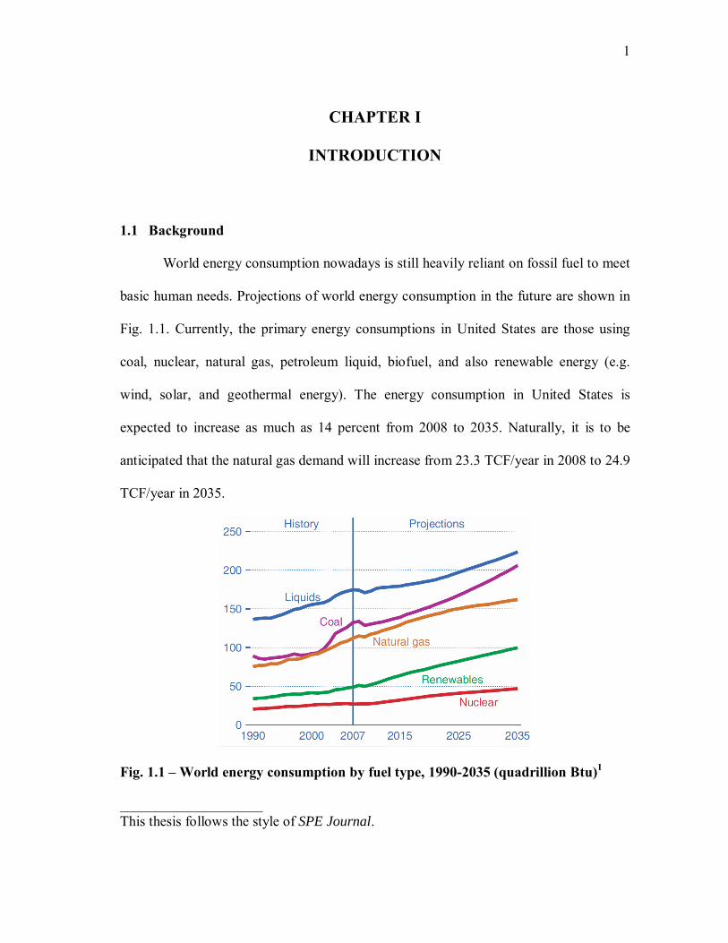
World energy consumption nowadays is still heavily reliant on fossil fuel to meet
basic human needs. Projections of world energy consumption in the future are shown in
Fig. 1.1. Currently, the primary energy consumptions in United States are those using
coal, nuclear, natural gas, petroleum liquid, biofuel, and also renewable energy (e.g.
wind, solar, and geothermal energy). The energy consumption in United States is
expected to increase as much as 14 percent from 2008 to 2035. Naturally, it is to be
anticipated that the natural gas demand will increase from 23.3 TCF/year in 2008 to 24.9
TCF/year in 2035.
Fig. 1.1 – World energy consumption by fuel type, 1990-2035 (quadrillion Btu)1 ____________________ This thesis follows the style of SPE Journal.

2
To meet the demand, natural gas production needs to be intensified from 20.6
TCF/year in 2008 to 23.3 TCF/year in 20352. The unconventional gas reservoirs (tight
gas, shale gas and coalbed methane) have evolved into important sources for the total
natural gas production in United States, and, therefore, will also be dominating the
natural gas sources by 2035 (Fig. 1.2).
Fig. 1.2 – Energy consumption in US, 1980-2035 (quadrillion Btu)2
Unconventional gas reservoirs have contributed a significant amount of gas
production in United States. These unconventional reservoirs, such as tight gas, shale gas
and coalbed methane in terms of reservoir occurrence, are different from the
conventional reservoirs (e.g. sandstone, carbonate). One of its distinctions is that the
source rock of unconventional reservoir also acts as reservoir rock3. Another explanation
of unconventional reservoirs is the application of production technology enhancement
such as massive hydraulic fracturing in tight gas, horizontal well and multiple hydraulic

3
fracturing in shale gas, and steam injection in heavy oil reservoir. The point of such
practice is to achieve reservoir production at an economical flow rate at which it will not
be so economical to use the conventional production method4. Another distinction is its
occurrence. In some cases it is also referred to as a basin-centered continuous
accumulation where the hydrocarbon distribution is found in a large area. However, it is
very difficult to determine the water oil contact in an unconventional reservoir and it
tends to be abnormally pressured5.
Initially, coalbed methane came up as a safety issue in coal mining industry6. To
minimize risks caused by gas existence, a gas releasing mechanism was taken as an
operating procedure in coal mining industry. To produce gas before underground mining
operation is commenced, the mining operation utilized a well that was placed in the coal
seam.
The United States government’s policy then encouraged early unconventional
gas development including a coalbed methane reservoir. For instance, the Section 29 tax
credit3 that was initiated in 1980 and took place until 2002 has evoked investments in
early coalbed methane development. The tax credit improved the economic value of
coalbed methane development by implementing a subsidy of US$ 3 for each barrel (oil
equivalent). On the other side, the gas price increment since 1970 also actuated the early
coalbed methane reservoir development. A prediction of coalbed methane reservoir
contribution on natural gas supply in US is shown in Fig. 1.3.

4
Fig. 1.3 – Natural gas supply in US, 1990-2035 (trillion cubic feet)2
Gas in a coalbed methane reservoir is generated during coalification3 (a process
of coal formation from organic matures). During a coalification process, methane,
carbon monoxide, and other gases are produced and accumulated on the surfaces area of
the internal coal micropores system. The coal seam has the ability to adsorb methane for
a large quantity to have an economic value to be produced.
Based on gas generation mechanism, a coalbed methane reservoir is classified as
thermogenic and biogenic3. Gas generation by a thermogenic process is governed by
temperature effects during an organic matter transformation. On the other side, gas
generation by a biogenic process is a result of a microorganism activity during a
coalification process. Microorganisms transported by water are the source of organic
matters during the transformation process.

5
One advantage of coal as reservoir rock is its capacity to store gas on the internal
surface area of coal matrix. The ability of coal to store gas is much higher than a
conventional reservoir at an equal rock volume due to extensive surface in the
micropores of a coal matrix. Because of its characteristic of storing a larger amount of
gas in the adsorption state, coalbed methane has become attractive to be produced by
drilling well into the coal seam. A greater storage potential of a coal seam is achieved by
higher reservoir pressure. A higher reservoir pressure provides more capacity of coal
seam to hold the gas in the adsorption state on the surface area of internal micropores
system inside the coal seams. The sorption capacity of coal seam varies based on several
factors, such as rank of the coal, coal composition, micropores structure, reservoir
pressure, molecular properties of gas adsorbed on the internal surface of coal seam, and
reservoir temperature3,7.
An idealized model of coalbed methane reservoir consists of a matrix system and
a fracture system. A matrix system represents the storage of gas inside the coal seam and
a fracture system represents the fluid flow path in the coal seam. The behavior of
adsorbed gas inside the micropores is modeled by gas inside the matrix system. The
mechanics of fluid flow in the coalbed methane reservoir are governed by a cleat system,
a natural fracture developed during coalification. The cleat system consists of face cleats
network and the butt cleat network. Both natural fracture systems are interconnected and
act as fluid flow media outside the matrix system that deliver gas that has been released
from the matrix system to the production well. The gas released form the matrix system
is strongly related to pressure distribution inside the matrix system. Therefore, the

6
releasing mechanism of all the gas adsorbed inside the matrix system on the internal
surface area depends on the pressure at any time. Since a coalbed methane reservoir
modeling concept consists of matrix and fracture systems, the existing dual porosity
model concept is commonly applied in the coalbed methane reservoir modeling.
However, the fluid flow fundamentals in a matrix system of coalbed methane reservoir is
not governed by a potential gradient (Darcy’s law), it is more common to model fluid
flow inside a coalbed methane matrix system by a gas concentration gradient (Fick’s
law).
A mathematical model of a dual porosity system that is commonly applied in the
oil and gas industry is presented by Warren and Root8. The dual porosity model
represents fluid flow performance inside two different medias; the matrix and fracture
systems. With some modifications, the Warren and Root mathematical model has also
been adapted in unconventional gas reservoir, including the coalbed methane reservoir.
The main fluid flow path in the coalbed methane reservoir is the cleat system. An
idealized model of a cleat system in the coalbed methane reservoir as presented in Fig.
1.4 consists of the face cleats system and the butt cleats system. In the coal natural
fracture system, the fracture density depends on the thickness and ash content. Greater
fracture density occurs more commonly in thin coal than in thick coal. Ash content in
coal seam also influences the fracture density, bulk density and coal rank7. The stress
distribution available in the field during a coalification process influences the generated
fracture direction. The direction of continuous cleat or face cleat in the coal seam is
governed by stress orientation. Face cleat orientation tends to be perpendicular to the

7
minimum stress direction. Permeability anisotropy in the coalbed methane reservoir is
related to the developed cleat system.
Fig. 1.4 – Schematic cleat characteristics3 Methane production from a coal matrix can be achieved by lowering the
reservoir pressure or the partial pressure of adsorbed gas in a coal matrix. Gas desorption
occurs after the pressure declines until it reaches below the desorption pressure.
Therefore, coalbed methane production methods depend on how to reduce overall
pressure within the reservoir body by producing the formation water.
Water treatment technology in a coalbed methane operation was developed by
modifying conventional gas production facility. For instance, a separator design in
coalbed methane operation is prepared for formation water handling and separation of
solid content from coal mines. The main difference of water production characteristics in

8
coalbed methane is that it has a lower total of dissolved solids or in other words, it is
fresher than the conventional gas water production.
As water is produced from the wellbore, the pressure reduction starts to occur
around the wellbore. Pressure reduction disperses through a reservoir body until the
hydrostatic pressure reaches below the adsorption pressure, and at this condition
methane gas desorption starts to take place. After desorption occurs, methane gas starts
to migrate through permeable strata, especially the cleat system to the lower pressure
area toward the wellbore area. In the near-surface area, coal outcrops may experience
hydrostatic pressure reduction followed by desorption and gas migration through porous
media to the surface or are entrapped with groundwater.
Different with conventional gas production characteristics, coal bed methane
reservoir production performance has a unique production trend. At the beginning, when
the reservoir pressure is higher than the desorption pressure, no gas will be produced.
After the reservoir pressure declines and falls below desorption the pressure by
producing formation water, then gas starts to desorb. During this initial stage, the gas
production will increase until it achieves its peak production. After such peak
production, the production performance will be similar with the conventional gas
production. Conventional gas reservoir gas production behavior is related with pressure-
depletion in the reservoir, so after peak production it will decline until it does not have
any pressure or production pressure constraint. While the desorption process in a coalbed
methane reservoir is governed by pressure reduction in the reservoir, the driving
mechanism of gas methane flow in the cleat system is influenced by the difference of the

9
reservoir pressure and the wellbore pressure. The energy of a gas methane flow is
derived from the reservoir pressure. On the other side, the reservoir pressure reduction
helps gas methane to desorb from the matrix surface area. Coalbed methane reservoir
production strategy through pressure depletion is quite common in the industry and
about 50 percent of gas in place could be economically recovered by implementing the
depletion strategy9.
Gas in a coalbed methane reservoir is stored by adsorption mechanism. The gas
is attached on the internal surface area of the coal matrix. After the reservoir pressure
declines until it reaches below desorption pressure, gas starts to desorb from the internal
surface area of the coal matrix. The gas drainage mechanism may be explained better by
molecular diffusion (Fick’s law) rather than the fluid flow derived from the pressure
difference (Darcy’s law). The process of gas drainage according to the diffusion process
is related with sorption time. Sorption time is a value that represents a characteristic of a
drainage process which is the required time to desorb methane gas for a constant
pressure and temperature condition. A typical production performance of a coalbed
methane reservoir is presented in Fig. 1.5.
As shown in Fig. 1.5., the first stage of production profile is the dewatering
process. The dewatering process is a mandatory procedure in a coalbed methane
reservoir with higher reservoir pressure than the desorption pressure. Therefore, during
the initial production stage, the only fluid produced from the wellbore is formation
water. The fundamental of a fluid flow in this initial stage is exactly similar with
conventional gas reservoir, the water flows through the cleat system or any permeable

10
strata governed by Darcy’s law. Since water production has been initiated, reservoir
pressures start to decline. After the declining pressure reaches the desorption pressure,
methane gas starts to desorb.
Fig. 1.5 – Typical coalbed methane production behavior
As shown in Fig. 1.5., the first stage of production profile is the dewatering
process. The dewatering process is a mandatory procedure in a coalbed methane
reservoir with higher reservoir pressure than the desorption pressure. Therefore, during
the initial production stage, the only fluid produced from the wellbore is formation
water. The fundamental of a fluid flow in this initial stage is exactly similar with
conventional gas reservoir, the water flows through the cleat system or any permeable
strata governed by Darcy’s law. Since water production has been initiated, reservoir

11
pressures start to decline. After the declining pressure reaches the desorption pressure,
methane gas starts to desorb.
The gas resulted from desorption process causes a concentration gradient within
the matrix system. At this stage, Fick’s law is more appropriate to be used as a
fundamental equation of gas methane drainage phenomenon. Because reservoir fluid has
been recovered, the reservoir pressure declines and water production will also decrease.
As the water production decreases caused by lower reservoir pressure, gas production
increases resulting from the desorption process.
The gas rate will keep increasing until it achieves peak production. In this early
time, the gas production behavior is strongly related to the diffusion process. Eventually,
after reservoir pressure depletion becomes a more significant factor, the gas production
behavior will follow Darcy’s law. Therefore, gas starts to decline and the production
performance will be governed by the pressure gradient. Pressure reduction will also
influence permeability and porosity because a coal matrix tends to shrink at a lower
pressure condition. In this case, the porosity value will be lower and it will change the
reservoir permeability as well.
The gas production profile is different in the dry coal system. In this system, the
initial formation water does not exist in the reservoir. Therefore, gas production occurs
from the early well life and a dewatering process is no longer required. The production
profile is almost similar with a conventional gas reservoir. However, a desorption
process is still an important mechanism of the depletion strategy. One should consider a
desorption process after the reservoir pressure reaches a lower value than the desorption

12
pressure. At this stage, gas desorbs from the internal surface of the coal matrix and gas
drainage within the coal matrix starts to take place due to the gas concentration
difference (diffusion process). Afterward, gas starts to flow through the permeable strata
and the cleat system into the welbore. There are several papers available explaining the
production performance behavior in a coalbed methane reservoir considering the
complex relationships among adsorption, diffusion, and matrix shrinkage along the
reservoir life cycle.
1.2 Problem Description
In coalbed methane reservoir development plan, well spacing scenario is an
important issue to estimate overall project feasibility. In the other side, there are several
uncertainties in reservoir properties that should be taken into account during the decision
making process. The uncertainties include the coal density, permeability or gas content
as parameters of coal properties. Each coalbed methane reservoir property will govern
production performance in a certain degree. Some parameters strongly influence
production behavior, for instance coal matrix gas content or coal system effective
permeability. However there are also other parameters with less contribution than the
others on the alteration of overall gas production performance.
Economic calculation of each well spacing scenario depends on the prediction of
future production performance. Instead of randomly considering variation of possible
parameters, it is often necessary to perform a sensitivity analysis and parametric study to

13
select the most influential factors in the reservoir model that will determine future
production performance.
1.3 Objectives
This work intends to investigate the effects of coalbed methane reservoir
properties to reservoir development scenario especially the well spacing strategy.
Coalbed methane reservoir production performance is modeled by a reservoir
simulation. A reservoir simulator will be utilized to investigate and document the effects
of coalbed methane reservoir properties on the selection of well spacing scenario. A
parametric study and sensitivity analysis are performed on numerous combinations of
reservoir parameters. A screening procedure is also provided to guide parameters
selection in the sensitivity analysis and parametric study process. The effect of each
parameter variation is investigated to determine the influence of parameter uncertainty to
the gas flow behavior in the coalbed methane reservoir simulation model.
1.4 Organization of this Thesis
The study is divided into five chapters. The outline and the organization of this
thesis are as follows:
Chapter I presents an overview of coalbed methane reservoir. The research
problem is also described in this chapter as well as the project objectives.
Chapter II presents a literature review. This chapter gives the existing overview
about coalbed methane reservoir occurrence and development, fundamentals of the fluid

14
flow in a coalbed methane reservoir, coalbed methane reservoir modeling, and economic
modeling.
Chapter III presents fundamentals of coalbed methane reservoir engineering and
sensitivity study. The reservoir engineering approaches include gas storage mechanism,
the fluid flow in a coalbed methane reservoir, and the reservoir simulation. This chapter
also provides fundamentals of a sensitivity analysis and Monte Carlo simulation.
Chapter IV presents simulation results on a specific data set, the sensitivity study,
and an economic model. The evaluation includes well spacing effects. This chapter gives
insights about the decision making procedure, especially well spacing determination.
Chapter V presents the conclusions and future recommendations.

15
CHAPTER II
LITERATURE REVIEW
2.1 Introduction
It is common to consider a coalbed methane reservoir as a dual porosity or
naturally fractured reservoir. A coalbed methane reservoir is a naturally fractured
reservoir with a coal matrix that has the potency as methane gas storage. Storage
mechanism in a coalbed methane reservoir could be explained by an adsorption process.
An adsorption process enables gas to be attached on the internal surface area of the coal
matrix. On the contrary, with a desorption process, methane gas is released and gas
drainage occurs, which allows gas to be transported through permeable media or a
fracture system. A fracture system in the coalbed methane reservoir is strongly related
with the cleat system. The fracture system, in this case the face cleat and butt cleat, acts
as a porous medium and cause reservoir anisotropy. The face cleat is more continuous
and longer than the butt cleat, and it tends to exist continuously through the reservoir
body. On the other side, the butt cleat is a perpendicular fracture that is shorter and
discontinuous. The butt cleat is discontinuous because during natural fracture formation
it is intersected by face cleats. Face cleats tend to be more continuous because they are
first-formed fractures and are more systematic. The butt cleat is a secondary natural
fracture system and is less systematic during its development than the face cleats, so this
natural fracture system contributes to the reservoir anisotropy. The face cleats also
provide a larger interface area with the matrix system than the butt cleats do. This

16
phenomenon makes the face cleats more important in the fluid flow mechanism. It is
common to assume the face cleat direction as the maximum permeability direction.
However in some cases, this is not a correct assumption, such as in the case of Bowen
basin, Australia11.
The storage capacity of a coal matrix can be considered as a economic resource;
however the coal matrix permeability is very low. The coal fracture system, particularly
the cleat system, provides media for fluid flow in the coal system. The cleat system
contributes to overall formation permeability. Methane gas resulting from desorption
process flows through the cleat system or natural fractures into the wellbore. The
permeability anisotropy is related to the formation of face cleats and butt cleats, in this
case the anisotropy creates a preferential flow. It is more common to find the maximum
permeability orientation parallel with the face cleat direction. Furthermore, the drainage
pattern will also be determined by permeability anisotropy.
2.2 Dual Porosity Model
The first dual porosity model was introduced by Barenblatt, G.I., Zheltov, I.P.,
and Kochina, I.N.10. A further development of a dual porosity model was then presented
by Warren and Root8, who proposed the application of a dual porosity model in well
testing interpretation. The Warren and Root dual porosity model later became a basic
concept in the development of naturally-fractured reservoir characterization techniques.
Most unconventional reservoirs for gas such as tight gas, shale gas, and coalbed methane
are classified as naturally-fractured reservoirs. As shown in Fig. 2.1, Warren and Root

17
proposed a conceptual model for a naturally-fractured reservoir by modeling a
homogeneous matrix block that is separated by fractures. The matrix block serves as
storage for adsorbed gas and the fracture system provides media for the fluid flow within
the reservoir body, from the matrix to the fracture system, which is followed by the fluid
flow from the matrix system to the wellbore. The overall formation permeability is
strongly related with a fracture or cleat system.
Fig. 2.1 – Schematic of dual porosity model8
The dual porosity concept proposed by Warren and Root is also applicable in a
coalbed methane reservoir. The dual porosity concept provides an idealized model of
reservoir performance in two different types of media. The first medium is storage that
contributes to the pore volume but with very low flow capacity. The second medium is a
fracture system which contributes to fluid flow. Warren and Root classified porosity into

18
two categories. The first one is the primary porosity controlled by deposition and
lithification. The second type of porosity is the secondary porosity; a porosity that is
controlled by water solution, natural fracturing, and jointing. A mathematical model for
this description is presented for the application of a pressure build-up analysis. The
idealized model is derived at an unsteady state condition and presented with two
additional parameters to characterize the dual porosity system. The two additional
parameters are ω and λ. The first parameter, ω, serves as a model fluid capacitance. This
parameter is introduced as storativity, a measure of fracture system storage capacity. The
second parameter, λ, refers to the heterogeneity exists in the dual porosity system. This
parameter is introduced as an interporosity flow parameter or flow capacity. The
mathematical model presented by Warren and Root is derived at a pseudosteadystate
condition (semisteadystate or quasistedystate). An equation for this interporosity flow
from the matrix system to the fracture system in a mathematical point is presented as
fmm ppkq
An application of the mathematical model was prepared for pressure buildup analysis.
Pressure buildup data show parallel lines on a semilog plot. The parallel lines are
separated by a transition with S-shaped. The first line represents the fluid flow in the
fracture system. After the transition period occurs, the second line appears as a
representation of the total system behavior (both of matrix and fracture system).

19
2.3 Coalbed Methane Reservoir Modeling
Previous studies have investigated the effect of coalbed methane properties
variance on the production performance. David, Turgay, Wonmo and Gregory11
presented a mathematical model to simulate methane and water flows through the coal
seam and the effect of coalbed methane reservoir properties on gas drainage. This work
uses single and multiple well systems. Olufemi, Turgai, Duane, Grant, Neal et al.12
conducted numerical reservoir simulations to study the effects of coal seam properties
variability in an enhanced coalbed methane project. They used a numerical simulation
model to show the most influential parameters that affect recovery in an enhanced
coalbed methane reservoir project. However, most of these works did not cover the
development of fundamentals of the fluid flow and adsorption-desorption phenomenon
in numerical modeling.
Cervik13, in 1967, presented a basic concept of transport phenomenon for gas at a
free gas and desorption state. This work showed gas dependency of gas desorption
phenomenon to the coal particle size, equilibrated pressure and diffusivity coefficient. It
showed that smaller particle tends to provide more gas. He proposed three classifications
of gas transport phenomena. The first one was principally Fick’s law while the second
one was a combination of Fick’s and Darcy’s law, and the third one was predominantly
Darcy’s law. Base on the results, it was not recommended to use the same basic concept
for conventional gas reservoir engineering in a coalbed methane reservoir model, since
the Darcy’s law and Fick’s law govern overall mass transport phenomenon.

20
By using a numerical simulator, Zuber, M.D., Sawyer, W.K., Schraufnagel, R.A.,
and Kuuskaraa, V.A.14 illustrated the procedure to determine coalbed methane reservoir
properties by using a history-matching analysis. The numerical simulator was modified
to adjust the flow and storage mechanism in a coalbed methane reservoir. In the history-
matching process, a two-phase dual porosity simulator was used to model reservoir
performance based on production data, geological data, and laboratory data.
Another work conducted by Seidle15 presented a methodology to utilize a
conventional reservoir simulator with some input data modification to model a coalbed
methane reservoir. This work assumed an instantaneous desorption that occurred from
the matrix block to the cleat system by using the analogy of dissolved gas in immobile
oil for a conventional reservoir simulator as adsorption gas on the internal surface of a
coal matrix. This work showed that the rate of diffusion in the matrix system was much
higher than the fluid flow in the cleat system. Therefore, this work analogizes gas
adsorption as saturated gas in immobile oil. In this case, the solution gas oil ratio is
determined by the Langmuir isotherm equation.
Fig. 2.2 shows the correlation between gas content and pressure. A modification
relative permeability curve is proposed to account the pseudo oil. The modification of
input data is applied on porosity and relative permeability curves (gas-water systems)
considering the existence of the immobile oil. However, this work did not modify basic
equation in the simulator. The works were verified by comparing a commercial
simulator for black oil with a coalbed methane reservoir simulator.

21
0
50
100
150
200
250
300
350
400
450
500
- 1,000 2,000 3,000 4,000 5,000 6,000 7,000 8,000 9,000 10,000
Pressure, psi
Gas
Sto
rage
Cap
acity
, scf
/ton
Lagmuir Volume, VL, saturated monolayer
Fig. 2.2 – Langmuir isotherm curve
Another work on conventional gas reservoir engineering adapted to coalbed
methane reservoir was presented by King16. His work showed a modification of material
balance concept for reserve estimation and prediction of future production performance
in unconventional gas reservoirs. This work utilized fundamentals of conventional gas
reservoir engineering for material balance techniques in a coalbed methane reservoir
with the effects of gas desorption and diffusion in consideration. The material balance
analysis assumed an equilibrium state of gas and adsorbed gas in the coal system. A
pseudo-steady state condition was also assumed to be applied during the sorption
process. This work provided a procedure of gas in place estimation by using the p/z
method and prediction of future production performance based on the existing material
balance techniques.

22
A modification of King’s method was presented by Seidle17 with more advanced
techniques in material balance. His work provided fundamentals of a mathematical
model, simulation studies, and examples of field application. The modified method
improved material balance techniques by eliminating mathematical problems and
suggesting more accurate reserve estimation for a coalbed methane reservoir.
Other numerical reservoir simulation studies were presented by David, H. and
Law, S.18, Hower, T.L.19, and Jalal, J. and Shahab, D.M.20. They showed the application
of a compositional simulator in coalbed methane reservoir modeling. The numerical
compositional simulator was equipped with some additional features for coalbed
methane reservoir modeling. David and Law’s work showed coalbed methane enhanced
the recovery model by using a compositional numerical simulator. The enhanced
recovery method is the CO2 injection. The compositional simulator was able to model
more than two components. This work assumed instantaneous process of gas diffusion
from the matrix system to the fracture system.
Aminian, K., Ameri, S., Bhavsar, A., Sanchez, M., and Garcia, A.21 presented
another approach of predicting coalbed methane gas production performance by using a
type curve matching based on gas and water rates. This method used dimensionless rate
and time. It also showed the application of the type curve matching for determining the
matrix and cleat porosity based on production- history matching. Based on the matching
results, future production performance could be estimated to evaluate the coalbed
methane reservoir prospect. This study also provided a correlation of the peak gas rate to
predict future production performance.

23
A later work by Reeves, S. and Pekot, L.22 presented a mathematical model for a
desorption-controlled reservoir. They introduced the model as a triple-porosity dual-
permeability model. This mathematical model was a modification of Warren and Root’s
model. This work showed the erroneous result of the previously existing dual-porosity
single-permeability model in predicting coalbed methane reservoir performance. An
overestimation of gas and water production tended to appear with the inconsistency of
the model result and field data. In fact, gas production was found much higher than the
gas predicted form the model in later time. To model this phenomenon, a set of porosity
and permeability was added to the system. The third porosity was introduced in the
matrix block system to provide free gas and water storage capacity for the modification
of material balance techniques. This work also provided decoupled models of a
desorption process from a matrix block and the diffusion process through a micro-
permeability matrix so that mass transport could be explicitly determined. A comparison
of the existing model result and the proposed model result was shown with a higher
water rate and lower gas rate which were more accurate and matched with field data.
This work also introduced a new coalbed methane simulator, COMET2 with some
modifications in the fundamentals of the fluid flow and desorption process.
A modification of Seidle15 approach was presented by Thomas, Tan.23, in 2002.
His work also used a commercial simulator to model coalbed methane reservoir
performance with independent implementation. He also showed a comparison of his
result in a paper by Paul, G.W., Sawyer, W.K,. and Dean, R.H.24. This work illustrated
pressure dependent porosity and permeability phenomenon with some comparative runs.

24
The result was not consistent with Seidle’ paper, but, as reported, it was an excellent
match for Paul’s paper. Tan’s work also suggested the dual grid approach to gain a more
accurate result in a matrix-fracture model.
In 2003, Xiao Guo, Zhimin Du, and Shilun Li25 presented a more sophisticated
numerical simulator with 3 dimensional and two-phase flow calculation capability. The
new simulator improved coalbed methane reservoir characterization by including
transport phenomena in the coal micropores and fracture system. The gas resulting from
the desorption process was calculated with a sorption isotherm curve from the
experiments and calculation. Therefore, an equilibrium state of desorption process was
necessary to be considered.
2.4 Coalbed Methane Reservoir Sensitivity Study
David, Turgay, Wonmo and Gregory11 investigated the relationship between the
peak gas rate and the ability of a matrix system to desorb gas. They performed a
sensitivity study to observe the consistency of new reservoir simulator results. The study
included an investigation of absolute permeability, sorption time for the gas diffusion
rate, and relative permeability effects on methane recovery for various well spacing
scenarios. The sensitivity study incorporated the effects of reservoir property variation
on the drainage efficiency of gas in the coal matrix system. This work used a single well
model.
Another work by Olufemi, Turgai, Duane, Grant, Neal, et al12 investigated the
effect of coalbed methane reservoir properties on production performance in a enhanced

25
coalbed methane project. A reservoir simulator was used to model reservoir performance
and select most influential parameters affecting gas recovery. It showed that reservoir
permeability, coal density, and Langmuir volume were the most significant factors in
methane recovery of a CO2 sequestration study.
Derickson, J.P., Horne, J.S., Fisher, R.D., and Stevens, S.H.26 presented a
sensitivity study result for coalbed methane reservoir production performance in
Huaibei, China. This work investigated the effects of some fundamental coal properties
variation on the production rate. They concluded that coal permeability, gas content,
initial water saturation, and coal thickness were the most influential factors related to gas
production.
Roadifer, R.D., Moore, T.R., Raterman, K.T., Farnan, R.A., and Crabtree, B.J.27
conducted a comprehensive study with more than 100,000 simulation runs. The study
was aimed to perform a parametric study incorporated with a Monte Carlo simulation
analysis. Numerous combinations of reservoir properties, geological data, completion
and operation constraint were prepared in the simulation runs to investigate the effects
on production performance. Relative importance of each parameter and inter-parameter
relationship were identified. Rank correlation was developed based on simulation results
considering several production constraints, such as the peak gas rate, dewatering times,
and cumulative gas production. Core sample acquisition in coal seams was difficult due
to its tendency to be extremely friable. This friability complicated the reservoir
properties measurement especially for permeability, porosity, compressibility and
relative permeability data. This paper explained the differences between a sensitivity

26
study and a parametric study based on basic concepts. The sensitivity study was
performed by changing one value while keeping the other values at the base value. On
the other side, a parametric study was conducted by preparing all possible combinations
of each parameter at every value (e.g. minimum, most likely, and maximum).
Stevenson, M.D., Pinczewski, W.V., and Downey, R.A.28 conducted a sensitivity
study for a nitrogen-enhanced coalbed methane study. This work investigated the effects
of reservoir parameter variation on the project economics based on predicted gas
production. The reservoir parameters that were identified as the most significant factors
were permeability, relative permeability, compressibility, layering and capillary
pressure. For each parameter, the minimum, most likely, and maximum values were
taken into account. San Juan basin data were chosen to be used in performing the
sensitivity study.
Reeves, S.R. and Decker, A.D.29 performed a discrete parametric study for a
wide range of the reservoir depth, pressure gradient, Langmuir volume, and permeability
as a function of pressure and depth. Young, G.B.C., McElhiney, J.E., Paul, G.W., and
McBane, R.A.30 presented a distinct parametric study for San Juan basin area. This work
divided San Juan basin into three areas for a discrete parametric study based on reservoir
properties variations. For instance, in Area 1 the sensitivity study covered permeability,
porosity and drainage variation. In Area 2 permeability, porosity, drainage area and
fracture half-length were investigated for a particular range. In Area 3, a sensitivity study
was performed for the coal compressibility, gas content, Langmuir parameter and
relative permeability ratio.

27
2.5 Well Spacing Effect
In a coalbed methane reservoir, well interference effect improves the pressure
reduction process by dewatering formation fluid from a cleat system. Interference
between coalbed methane wells causes the decline of reservoir pressure and helps the
initiation of the gas desorption process. Unlike a conventional gas reservoir, well
interference in a coalbed methane reservoir is an advantageous condition. David,
Turgay, Wonmo, and Gregory11 performed a parametric study to investigate well
interference effect in a coalbed methane reservoir. They used a multiple-well system to
observe gas and water production performance related to well interference. This work
concluded that interference between coalbed methane wells improved the gas methane
desorption process from the matrix to the cleat system by adding the pressure drawdown
in the coal matrix system. On the other side, water production performance tended to
show similar behavior for well interference effect in a conventional gas reservoir.
Another well-spacing study was conducted by Young, G.B.C., McElhiney, J.E.,
Paul, G.W., and McBane, R.A.31 by using a numerical reservoir simulation for Fruitland
coals in Northern San Juan Basin. This work showed the increment of methane gas
recovery factor in a reservoir model with smaller well-spacing. This work also included
fracture half-length as a variable in determining the most optimum development
scenario. The optimum well-spacing and fracture half-length depended on coalbed
methane reservoir variability. Young, G.B.C., McElhiney, J.E., Paul, G.W., and
McBane, R.A.31 continued their study with an investigation on well spacing effects on
the early peak production and gas decline rate. The study showed that the initial peak gas

28
rate tended to be higher in smaller well-spacing. On the other side, the gas decline rate
was higher in a smaller well-spacing scenario.
Another well-spacing study was conducted by Wicks, D.E., Schewerer, F.C.,
Militzer, M.R., and Zuber, M.D.32 in Warrior basin coalbed methane reservoir. To
investigate the effects of well spacing on methane recovery, they compared production
performance of 8 wells in 160 acres with 1 well in the same area. Their study found that
smaller well-spacing (8 wells in 160 acres) yielded 85 percent methane gas recovery
while 1 well in 160 acres only gave 25 percent methane gas recovery. However, this
work did not include economic factors on selecting the most optimum well-spacing
scenario.
Chaianansutcharit, T., Her-Yuan Chen and Teufel, L.W.33 also presented well
interference effects in coalbed methane reservoir production performance. They used a
numerical simulator to model coalbed methane reservoir performance for various well-
spacing scenarios. Their study showed that methane gas recovery tended to be higher in
a two-well system than a one-well system. This means that, unlike in a conventional gas
reservoir, interference effects would accelerate gas production.

29
CHAPTER III
COALBED METHANE RESERVOIR MODELING
3.1 Introduction
To characterize a coalbed methane reservoir, a dual porosity reservoir concept
can be applied. A coalbed methane reservoir consists of a matrix system and a fracture
system. The matrix system basically provides gas storage capacity in the internal surface
of coal micropores. During the coalification process, methane gas is adsorbed on the
internal surface area of coal. Due to the adsorption phenomena and low pressure system,
the fundamentals of characterizing a coalbed methane reservoir are different from that of
a conventional gas reservoir.
The fracture system is a conduit of a fluid flow after methane gas is desorbed
from coal matrix. A coalbed methane reservoir facture system is categorized into two
major natural fracture systems. The longest and a more continuous natural fracture
system is the face cleat. The shorter and more discontinuous fracture system is the butt
cleat system. The butt cleat system direction is perpendicular to the face cleat direction
and therefore intersected by the face cleat system. Since the face cleat contact area to
matrix system is larger, the gas drainage process is more prominent in face cleat contact
area. Therefore, the face cleats contribute more on the methane gas fluid flow. An
example of a coal cleat system is shown in Fig. 3.1.

30
Fig. 3.1 - Structure of coal cleat system4
To develop an adequate coalbed methane reservoir model, it is necessary to have
understanding about physical properties of a coalbed methane reservoir parameter and its
relationship on the desorption mechanism, diffusion process and fluid flow inside the
coal cleat system. This chapter will introduce the fundamental theories that govern the
coalbed methane reservoir performance behavior.
3.2 Gas Storage in Coalbed Methane Reservoir
The gas storage mechanism in a coalbed methane reservoir is different from the
one in a conventional gas reservoir. The methane gas is formed during the coalification
process, coal formation from plant material conversion. During the coalification process,
methane occurs as a byproduct and is adsorbed into the internal surface of the coal
micropore system. Therefore, a coalbed methane reservoir is also considered as both
source rock and reservoir rock.
Most of the gas is stored in a coalbed methane reservoir by an adsorption
process. The main driving force of an adsorption process is molecular attraction (Van

31
Der Walls forces). The physical of an adsorption process is governed by intermolecular
attraction between gas molecules and solid surfaces of the coal micropore system. Gas
methane is also present in a coalbed methane reservoir in several different ways. It can
be free gas compressed in the micropores system. Gas can also exist as free gas in the
pore system (where the pores are bigger than micropores) and the fracture system.
Another way of gas storage is dissolved in formation water.
As free gas, the methane gas is stored in the pore spaces. A normal gas law
principle can be applied in this condition; therefore, the amount of free gas can be
estimated by knowing the porosity and pressure value. The amount of free methane gas
is very small compared the adsorbed gas.
The coalbed methane storage capacity is much higher than that of a conventional
gas reservoir at an equivalent pressure and temperature condition. This characteristic
makes a coalbed methane reservoir is attractive to be exploited. The internal surface area
of the coal matrix micropore system is very large, and, thus, it enables more gas to be
stored at adsorption condition. For some coal types, the internal surface area of the
micropore system can reach hundreds of square meters per gram of solid12. The coal
seam capacity to store gas is 6 to 7 times higher than that of sandstone at the same
equivalent depth7.
The coal seam gas storage capacity is a function of pressure within the micropore
system. The amount of adsorbed gas is controlled by the free internal surface area of the
coal micropore system. The Langmuir adsorption isotherm curve can be used as a
function to estimate the adsorbed gas at a given pressure with a constant temperature

32
condition. The Langmuir adsorption isotherm curve is a reservoir parameter that
represents the amount of gas that will be desorbed if the reservoir decreases until it
reaches a value below the desorption pressure. Each time the gas is released, the gas
concentration at a given point will decrease and there will be an equilibrium state
between the pressure and the amount of adsorbed gas. Theoretically, at the zero pressure,
all the adsorbed gas will be released from the surfaces area of the internal coal
micropores system.
3.3 Gas Transport Mechanism
At the initial condition, most of the methane gas is adsorbed on the internal
surface area of the coal matrix micropore system. Generally, the fracture system is only
saturated with formation water with negligible soluble gas. Unlike a conventional gas
reservoir, only a very small amount of gas is stored as free gas in the pore system.
Therefore, to release adsorbed gas, the pressure inside the coal seams system
should be reduced until it reaches a lower value than the desorption pressure. The first
stage of coalbed methane production is initiated by producing formation water only. This
procedure is often named as a dewatering process. By producing formation water from
the cleat system, reservoir pressure will be decreased in proportion to the volume of
water removed from the cleat system.
After the matrix pressure system reaches a value lower than the desorption
pressure, the adsorbed gas on the internal surface area of the coal matrix micropore
system starts to desorb into the cleat system. The volume of released gas follows the

33
Langmuir isotherm curve and alters gas concentration at a given point. Because of the
presence of a gas concentration gradient, the diffusion process from the matrix system to
the fracture system begins to occur. Once the released gas enters the natural fracture
system, it flows through the cleat system into the wellbore. To summarize, there are
three main processes of gas transport phenomena in the coalbed methane reservoir
system. The first process is desorption when gas is released from the surfaces area of the
internal coal micropores system. Afterwards, the diffusion process takes place. Governed
by a concentration gradient, the desorbed gas flows from the coal matrix into the cleats
system. Finally, the gas flows through the permeable strata and the cleat system, which
is governed by the pressure gradient.
The gas transport phenomenon in a coalbed methane reservoir is measured by
two main parameters; the coal permeability and diffusivity. As the reservoir decreases,
the adsorbed gas is released from the surfaces area of the internal coal micropores
system. The releasing mechanism follows the desorption process. Since the micropore
size is very small, the gas is transported at a very slow rate and is governed by the
difference of gas concentration. In a very small micropore system, the gas flow rate
follows the diffusion rate rather than the fluid flow mechanism explained by Darcy’s
law. The main reason of this phenomenon is the existence of drag force which is very
high in the very small pore throat size. The diffusivity term represents the gas diffusion
rate at a given point. The coal permeability determines gas the flow rate through
permeable strata or the cleat system.

34
Fig. 3.2. shows three main processes in the coalbed methane transport
phenomena. The matrix is the micropore system while the fracture is the macropore
system. The fluid flow in each system follows different mechanisms. The desorption
process occurring in coal particles releases methane gas from the internal surface area of
the coal matrix. The diffusion process enables gas to be transported through the
micropore system. Eventually, fluid flows occur within cleat system which is governed
by the pressure gradient of the well being produced.
Fig. 3.2 - Methane flow dynamics11
Gas transport phenomena at diffusion state can be calculated using Fick’s law34.
At this stage, the gas is transported from the coal matrix micropore system into the
fracture system. The coal matrix micropore system is the primary porosity system. In
this system the main driving force of the diffusion process is the gas concentration
gradient. In the secondary porosity system or fracture system, the fluid flow is governed
Desorption from coal particle
Diffusion in micropores
Laminar flow in cleat system

35
by Darcy’s law or the pressure gradient. These two transport phenomena are different
from each other and yet they are interdependent on each other.
Jochen, V.A., Lee, W.J., and Semmelback, M.E.35 presented the fundamental
equation of the transport phenomena in the secondary porosity system or the macropore
system. In the macropore system or the cleat system, the transport phenomena of water
and gas are quantified using the following equation:
g
gg
gg
g
BS
tq
rp
rB
Krr
1
whereas the flow rate (q) is formulated as:
tCFq g
3.1
In this equation, q represents the pseudo-steady state diffusion rate at two given points.
The diffusion rate is determined by Fg, a dimensionless shape factor. Each shape factor
value represents a different micropore matrix geometry. The diffusion rate is the rate of
released gas flows to the fracture system; this phenomenon is governed by the gas
concentration gradient. The gas concentration gradient could be expressed by the
following equation:
fs pCCDFtC __
3.2
In this equation, __
C is the gas concentration (average in the coal matrix system) and the
C(pf) is the gas concentration (in the fracture system). The gas concentration at a

36
particular time step is calculated by using a material balance equation. Combining Eqn.
3.1 and Eqn. 3.2, the diffusion rate terms can be illustrated by the following equation:
fsg pCCFDFq
__
where Fs is shape factor for the primary porosity system. In this equation the product
FgDFs also represents the desorption time or the time constant for the pseudo-steady
state condition, written as τ. The desorption time is formulated as:
sg FDF1
By using the desorption time term, the equation for diffusion or desorption state is:
fpCCq
__1
The desorption time is a value representing a characteristic of a drainage process which
is the required time to desorb 63.2% of the ultimate drainage for a constant pressure and
temperature condition36. This parameter, (τ), represents the required time for gas to be
released from the surfaces area of the internal coal micropores system and transported to
the fracture (macropore system). In coalbed methane reservoir modeling, it is more
common to quantify the diffusion rate using the desorption time rather than the
diffusivity value. Practically, desorption time data could be determined by a laboratory
test called the canister test. In this test, coal core samples are placed in a desorption
canister equipment and equilibrated to a given temperature while measuring the
desorbed gas as the pressure system is decreased at any consecutive time.

37
Another expression of the diffusion process is presented by using a shape factor.
The drainage rate governed by Fick’s law can be quantified using the following
equation.
fc CCDq
__* ..
where q* is the drainage rate per volume of the reservoir. The relationship between the
desorption time (τ), shape factor (σ) and diffusivity coefficient (Dc) can be expressed by
the following equation:
cD.1
3.3
After the desorbed gas is released and transported to the fracture system
(macropores), the fluid flow is then governed by Darcy’s law. The fluid flow within this
fracture system can be described as the following equation:
dLdpAkq
As shown in this equation, the main driving force of fluid flow through fracture system
is the pressure gradient. This is the main difference between the transport phenomena in
the matrix system (micropores) and the fracture system (macropores). Although the gas
transported from the matrix system follows the concentration gradient (Fick’s law), the
amount of gas desorbed depends on the system pressure. The amount of gas released at
every pressure value follows the Langmuir isotherm curve.

38
3.4 Adsorption Isotherm
Methane gas is stored in the coal matrix by an adsorption process. The amount of
gas adsorbed on the internal surface area of the coal matrix micropore system can be
very large since the coal is able to provide a tremendous internal surface area. An
analogy for the adsorption process is dust attached to a surface area of wood or glass.
The adsorption is governed by the weak attraction forces between molecules. Therefore
adsorption process is reversible. Absorption is a different process; it is less reversible
than the adsorption process. An example of an absorption process is when water soaks a
sponge. The adsorption process may be explained with the Langmuir isotherm curve.
The Langmuir isotherm theory perceives gas molecules attached on the surface area as a
single layer (monolayer).
The basic concept of Langmuir isotherm theory is that the rate of gas molecules
arriving and adsorbing on a solid surface area is proportional to the rate of gas molecules
leaving the solid surface area. The Langmuir isotherm curve is useful to predict the
amount of gas released at a given pressure lower than desorption pressure. For a gas
storage mechanism, Kohler, E.T. and Ertekin, T.37 presented the relationship between
storage capacity and the adsorption isotherm curve. In an adsorption phenomenon
conceptual model, the Langmuir isotherm curve theory is applicable in an
unconventional gas reservoir, including a coalbed methane reservoir. An example of a
Langmuir isotherm curve is shown in Fig. 3.3.
As the system pressure declines, the storage capacity decreases and a certain
amount of gas will be released from the matrix system. The maximum storage capacity

39
is the Langmuir volume, a saturated monolayer volume. At this value, all surface area
has been adsorbed by methane gas or the gas content at an infinity pressure value. The
Langmuir pressure is a pressure value at half of the Langmuir volume.
0
50
100
150
200
250
300
350
400
450
500
- 1,000 2,000 3,000 4,000 5,000 6,000 7,000 8,000 9,000 10,000
Pressure, psi
Gas
Sto
rage
Cap
acity
, scf
/ton
Langmuir Volume, V L , saturated monolayer
1/2 Langmuir Volume, 1/2 V L
Langmuir Pressure, P L , pressure at 1/2 Langmuir Volume
Fig. 3.3 - Sorption isotherm, gas content as a function of pressure
The amount of gas adsorbed on the internal surface area of the coal matrix
micropore system could be quantified using the Langmuir equation. The Langmuir
isotherm equation is described as the following:
L
L pppVpV
where V(p) is the gas content at any given pressure (scf/ft3), pL is the Langmuir pressure
(psi), p is the pressure in the matrix system (psi) and VL is the Langmuir volume (scf/ft3).

40
The Langmuir volume can be estimated since it asymptotically increases at higher
system pressure value. The Langmuir pressure is the pressure value at a condition when
the amount of adsorbed gas reaches half of its maximum storage capacity. The Langmuir
pressure determines the curvature of the Langmuir isotherm curve. At a lower Langmuir
pressure value, the isotherm curve will be lower. However, at any Langmuir pressure
values, all curves will coincide at the same value, which is the maximum mono-saturated
value.
The Langmuir isotherm equation quantifies the amount of gas released at a given
pressure. The gas concentration at a certain pressure is assumed in an equilibrium state.
Therefore, in the Langmuir isotherm equation the change of methane gas concentration
depends only on pressure reduction. The pressure reduction allows gas to be desorbed
and transported through the diffusion process in the micropore system. There is a
pressure value when the gas starts to desorb, which is called the critical desorption
pressure. If the pressure value is higher than the desorption pressure, the gas desorption
process will never be initiated. To reduce the matrix system pressure, formation water
should be removed from the fracture system by making a coalbed methane well.
Initially, the only produced fluid is formation water. The amount of water being
produced is proportional to pressure reduction. After the reservoir pressure system
achieves a lower value than the critical desorption pressure, gas starts to be produced at
an early low rate and it reaches the peak gas production after several years. This
phenomenon is different from a conventional gas reservoir, where the gas production
declines without having to wait for the dewatering process.

41
Fig.3.4. shows a typical coalbed methane production performance. The
production profile is typical for an undersaturated coalbed methane reservoir system. An
undersaturated coalbed methane reservoir has a higher initial reservoir pressure than the
critical desorption pressure. Therefore, a depressurizing stage is necessary to allow the
desorption process to initiate. After the desorption process occurs, gas desorbs until it
achieves critical gas saturation. At this time gas and formation water flow through the
natural fracture system into the wellbore.
Fig. 3.4 - Typical coalbed methane production performance behavior4 3.5 Coalbed Methane Reservoir Porosity
In coalbed methane reservoir, coal formation is considered as both source rock
and reservoir rock. During coalification, methane gas is formed and stored in the same
media. Unlike in a conventional gas reservoir, where gas migrates from source rock to

42
reservoir rock, in this unconventional gas reservoir the methane gas is trapped at the
same place where it is originated from. In a conventional gas reservoir, the gas is stored
in the pore system or void between solid particles. On the other hand, coal is a solid
substance with micropore systems inside the coal matrix, surrounded by the natural
fracture system or cleat system. In a coalbed methane reservoir, only a small amount of
gas is stored as free gas in the pore system. Most of the gas stored as adsorbed gas in the
matrix micropore system. The coal micropore system provides a tremendous surface
area for methane gas to be stored during the adsorption process.
Basically there are three types of the coal pore system. The first type is the
natural fracture system or the cleat system, including the face cleats and butt cleats. This
pore system allows gas to be transported from the coal matrix into the wellbore with the
pressure gradient as a driving force. Another type is the interstitial pore space in the coal
matrix system. In this pore type, gas is stored as free gas inside the pore throat. The coal
matrix also has another type of porosity, the micropore system. The micropores are very
small in size yet able to provide a large amount of surface area to attach gas molecules.
3.6 Coalbed Methane Reservoir Permeability
A coalbed methane reservoir is commonly identified as a naturally-fractured
reservoir. Coal seams consist of the matrix system and fracture system. The matrix
system is the main methane gas storage but with very low permeability. Since the
permeability value is very low, it is often neglected in the modeling concept. Even when
gas transport phenomena occur in the matrix system, the gas drainage rate is very slow

43
and is dominated by the diffusion process (Fick’s law) instead of the fluid flow through
permeable media (Darcy’s law). Therefore, in a coalbed methane reservoir the
permeability concept is only applied in the fracture system. The coal permeability in the
fracture system determines how fast the depressurizing process will take place by
removing formation water from the fracture system.
3.7 Coalbed Methane Reservoir Saturation
In coalbed methane reservoir modeling, a gas and water saturation concept is
only applied in the coal micropore system. A coalbed methane reservoir consists of a
macropore system (fracture or cleats) and a micropore system (coal matrix). Initially, the
fracture system is fully saturated with water. It is common to neglect gas presence in this
early stage. After the desorption process begins, gas saturation in the fracture system
increases until it reaches the critical gas saturation. After achieving gas saturation value
higher than the critical gas saturation, methane gas starts to flow from the fracture
system into the wellbore and is exploited through surface facilities. Therefore, in a
coalbed methane reservoir, saturation terms refer only to the fracture or cleat system.
3.8 Coalbed Methane Reservoir Permeability Anisotropy
There are numerous authors who have introduced the existence of permeability
anisotropy in a coalbed methane reservoir. The main path for the fluid flow inside the
coal seam is the cleat system. Since there are two kinds of cleat systems in a coalbed
methane reservoir, the direction of permeability is complicated. The face cleat is more
continuous and it contributes a larger surface area for a gas drainage process from the

44
matrix system to the fracture system. The face cleat direction is perpendicular to the butt
cleat direction. The butt cleat system is the shorter natural fracture system intersected by
face cleat systems. Therefore the existence of face cleats system and butt cleats system
yield permeability anisotropy in the coalbed methane reservoir system. The well pattern
should consider permeability anisotropy in order to obtain the most optimum drainage
within a reservoir body.
Some authors have presented the significance of permeability anisotropy in
drainage pattern. Wicks, D.E., Schewerer, F.C., Militzer, M.R., and Zuber, M.D.32
presented a drainage pattern and methane gas recovery in a coalbed methane reservoir.
Based on their result, the rectangular drainage pattern increases methane gas recovery up
to 15 percent compared to the square pattern. Bumb, A.C. and McKee, C.R.38 also
presented the beneficial effect of designing a well pattern with the permeability
anisotropy in consideration. They showed that an appropriate well pattern would
increase the effectiveness of dewatering process.
Sung, W., Ertekin, T., and Schewerer, F.C.39 used a numerical reservoir
simulator to study the effect of well trajectory direction to methane recovery. They
proposed to drill a vertical well in the face cleat direction to improve methane recovery.
Another study by Young, G.B.C., McElhiney, J.E., Paul, G.W., and McBane, R.A.30
showed the importance of a permeability anisotropy study in developing a coalbed
methane reservoir in Cedar Hill Field, Northern San Juan Basin. Following their study
result, methane gas recovery can be improved by designing well placement with the

45
permeability anisotropy in consideration. They used a numerical simulator to model
permeability anisotropy and coalbed methane reservoir production performance.
Chaianansutcharit, T., Her-Yuan Chen, and Teufel, L.W.33 also studied the
permeability anisotropy effect on methane recovery in a coalbed methane reservoir.
They also introduced the dual peak gas rate behavior caused by boundary effects. The
dual peak gas rate occurs in a coalbed methane reservoir system with several boundaries
with different required times to achieve the boundary effect. They also suggested using
a rectangular drainage pattern in a coalbed methane reservoir development strategy.
3.9 Numerical Reservoir Model
Naturally fractured reservoir model consists of two different sub-systems: the
matrix system, which contributes to pore volume, and the fracture system, which is the
main path for the fluid flow. These two sub-systems are dependent on and
interconnected with each other. This concept is known as a dual porosity model. The
matrix system and fracture system have distinct characteristics, as presented by Warren
and Root in 19638. They introduced an idealized model for the dual porosity system.
However, there is a distinguished concept in a coalbed methane reservoir. Unlike in a
conventional gas reservoir, the matrix system has very low permeability.
The gas transport phenomenon in a coalbed methane matrix system is different
from the fluid flow mechanism in the fracture system. The gas drainage rate is very low
and dominated by the diffusion process. Therefore, to accommodate these unique
characteristics the Warren and Root model should be modified in coalbed methane
reservoir modeling. The modified dual porosity model should take into account the

46
diffusion process from the matrix system to the fracture system. This physical process
can be quantified by Fick’s law. Unlike the dual porosity model in a conventional
reservoir, the dominant driving force in matrix system is the gas concentration gradient.
In a conventional gas reservoir, the fluid flow mechanism in the matrix system
depends on the matrix pressure and the gas saturation in the matrix system. However, the
gas releasing mechanism in a coalbed methane reservoir depends on pressure. As the
matrix pressure declines, more gas will be released from the internal surface of the
matrix micropore system.
Even though the dual porosity concept is applicable in a coalbed methane
reservoir, the fundamental is different. Referring to the dual porosity concept, the matrix
system also contributes to the fluid flow although the porosity and permeability value is
very low. In a coalbed methane reservoir, the porosity and permeability concept is not
appropriate to be used in the matrix system. The effective permeability and porosity in
the coal matrix system is negligible. However, the matrix system is the main source of
methane gas. The drainage process refers to methane transport phenomena in the matrix
system depending on gas concentration gradient. The gas concentration depends on
system pressure. Considering that the matrix system only contributes in gas source
terms, a coalbed methane reservoir can be modeled by the single porosity system
coupled with the pressure-dependent gas source term.
An idealized model of a coalbed methane reservoir system is shown in Fig. 3.5.
A picture of an actual coal seam is presented in the left side. A face cleat is a continuous
fracture system longer than a butt cleat. The butt cleats are shorter and intersected by

47
face cleats. To build a reservoir model the cleats system is presented by a systematic
array of matrix blocks surrounded by fractures.
Fig. 3.5- Idealized coal seam model based on the dual porosity concept. (a) an actual coal seam and (b) an idealized coal system model 4
The matrix block permeability is very low but it has a high gas storage capacity
at the adsorption state. The matrix storage capacity is very large due to its ability to
provide a tremendous amount of internal surface area for methane gas to be adsorbed.
The adsorption process depends on the matrix system pressure. The fracture system
permeability is much higher, provides the main path for the fluid flow, and has
negligible gas saturation.
This work uses CMG GEM, a two-phase compositional simulator to model
coalbed methane reservoir performance under various well-spacing scenarios. This
simulator is suitable for the gas diffusion model in the matrix system. A dual-porosity
model is used to calculate the mass transport phenomena between the matrix system and
the fracture system. In the matrix system, the desorption process is quantified by using

48
the Langmuir sorption isotherm theory. The fluid flow in the fracture system is modeled
by Darcy’s law. Instead of Darcy’s law, the matrix-to-fracture flow model uses the
diffusion theory. By understanding this concept, the permeability value in the matrix
system is redundant. On the other side, the matrix relative permeability data are also
redundant in the matrix system.
In CMG GEM, the dual-porosity model uses Gilman and Kazemi finite
difference equation40. The diffusion process is quantified by the gas concentration
gradient based on the Langmuir isotherm model. The gas drainage through the diffusion
process is calculated using the Fick’s law. On the other hand, the gas concentration
depends on the system pressure. Therefore, an equilibrium condition between gas
concentration at any given pressure and the drainage rate is calculated during the
iteration process or each time step. This simulator has also incorporated coal shrinkage
and compaction effect during the reservoir life.
The mass transport phenomenon from the matrix system to the fracture system or
diffusion process is unique for each coal type. A parameter called the desorption time (τ)
determines how fast the drainage process during diffusion process. The desorption time
could be calculated based on the diffusion coefficient, cleat spacing, and shape factor.
CMG uses Kazemi’s concept to calculate the shape factor. For a very low value of
desorption time, the diffusion process will be faster and the equilibrium state can be
achieved within a shorter time.
Even permeability and relative permeability data are not required for the matrix
system; the simulator needs input data for the dual-porosity model. The dual porosity

49
model consists of two different porosity systems. The primary porosity is the matrix
system and the secondary porosity is the fracture system. In coalbed methane reservoir
modeling, it is necessary to understand that the concepts of permeability and relative
permeability are only applied in the fracture system. The matrix system only provides
the gas source and the amount of released gas during the desorption process depends on
matrix pressure at a given time.
CMG GEM as a compositional simulator is able to provide a numerical
simulation model for a coalbed methane reservoir. However, one should be careful in
utilizing the dual-porosity concept in this simulator since it is different from its use in a
conventional gas reservoir. The mass transport phenomenon in the matrix system is
different from the conventional simulator where the permeability and relative
permeability values determine the fluid flow in the matrix system.
3.10 Sensitivity Study
To investigate and mitigate the risks in coalbed methane reservoir development,
one should have adequate understanding about relationship between the uncertainty of
reservoir properties and their impact on production performance. A sensitivity study is
widely used in the procedures of finding the relative importance of each parameters and
their inter-relationship. The main purpose of conducting this study is to build a rank
correlation between the parameters and the expected outcome (e.g. cumulative gas
production, recovery factor, original gas in place). There are several methods commonly

50
taken to perform sensitivity study, such as the One-Factor-A-Time method, the Placket
Burman method, and the Box Behnken method.
3.10.1 One-Factor-A-Time Approach
A sensitivity study is performed by changing one factor at a time while keeping
the other factors constant during calculation. This method has been quite popular
because of its simplicity and tendency to avoid mistakes during calculation. However,
this method is limited in term of its capability to investigate all extremities of input
parameters.
The extreme condition for some cases occurs when a combination of input
parameters is introduced. For example, gas production will increase with higher fracture
system permeability. The maximum effect of changing fracture permeability cannot be
observed only by changing the fracture permeability alone without changing other input
data. For this case, higher gas production can be obtained by maximizing the fracture
permeability and reservoir thickness. Table 3.1 shows an example of the One-Factor-A-
Time approach.
3.10.2 Plackett-Burman Approach
The Placket-Burman approach is categorized as a two-level factorial design. In a
two-level factorial design, there are two values of each parameter that will be taken into
account in a sensitivity analysis. Those values are the minimum value and maximum
value. For a complete combination, the n factor requires 2n experimental runs to consider

51
all possible combinations among all the factors. For example, to make sensitivity
analysis for 3 factors, one should prepare 8 experimental runs. The advantage of using
the Plackett-Burman design is to reduce the amount of experimental runs. The Plackett-
Burman design introduces a single generating vector to construct a certain number of
experimental runs. Table 3.2 shows generators used in Plackett-Burman design. The
minimum condition is symbolized by -1, while 1 means maximum condition41.
Parameter Minimum Most Likely MaximumThickness, ft 25 30 40
Matrix porosity, fraction 0.0125 0.005 0.2Fracture porosity, fraction 0.0025 0.001 0.04
Experiment Thickness, ft Matrix porosity Fracture porosity1 30 0.005 0.0012 25 0.005 0.0013 40 0.005 0.0014 30 0.0125 0.0015 30 0.2 0.0016 30 0.005 0.00257 30 0.005 0.04
Table 3.1 - Example of one factor at a time appoach
Number of Factors Number of Runs Generator4 - 7 8 1 1 1 -1 1 -1 -18 - 11 12 1 1 -1 1 1 1 -1 -1 -1 1 -1
12 - 15 16 1 1 1 1 -1 1 -1 1 1 -1 -1 1 -1 -1 -116 - 19 20 1 1 -1 -1 1 1 1 1 -1 1 -1 1 -1 -1 -1 -1 1 1 -120 -23 24 1 1 1 1 1 -1 1 -1 1 1 -1 -1 1 1 -1 -1 1 -1 1 -1 -1 -1 -1 -132 - 35 36 -1 1 -1 1 1 1 -1 -1 -1 1 1 1 1 1 -1 1 1 1 -1 -1 1 -1 -1 -1 -1 1 -1 1 -1 1 1 -1 -1 1 -1
Table 3.2 - Plackett-Burman design generator

52
3.10.3 Box Behnken Approach
When there are three conditions available in one parameter, a three-level factorial
design is required. Examples of the three conditions are the minimum value, the most-
likely value, and the maximum value. The Box Behnken method is one approach that is
categorized as a three-level factorial design. A three-level factorial design uses all
combinations among three factors. For a complete design, one needs to prepare 3n
Fig. 3.6 - Illustration of Three-level full factorial design experimental runs for n factor. For instance, 3 factors will need 27 experimental runs to
have a full factorial design. A graphical illustration of full factorial design is presented in
Fig. 3.6.
One of the advantages of using the Box Behnken method is that the required
experimental runs will be much less than a three-level full factorial design. The Box
Behnken method is also very useful in selecting fewer experimental runs to provide
responses of the main effect from each parameter. This method also considers

53
relationship between a parameter and all quadratic effects. The disadvantage of Box
Behnken method is its inability to investigate the extreme condition. Fig. 3.7 shows an
illustration of the Box Behnken approach.
Fig. 3.7 - Illustration of Box Behnken design
3.11 Monte Carlo Simulation
The Monte Carlo simulation has been widely used to accommodate uncertainties
in reservoir engineering. Each parameter has uncertainty. It is common to provide
reservoir data in a range of more than a single value. The Monte Carlo simulation can be
used to transform the uncertainty from a selected parameter to produce a distribution
function. Each parameter has a distribution function and when all the distribution
functions are combined, the result will be different. To sample a number of input data,
random numbers are generated. A graphical presentation is shown in Fig 3.8 to illustrate
distribution functions as a result from the Monte Carlo simulation.
There is a concession in the cumulative distribution function to have a
description about the expected value. The P10 (also being known as proven) value

54
represents a certain value where there is 10% possibility to acquire values less than the P
10 value. The same concept applies for P 50 (probable) and P 90 (possible).
Fig. 3.8 - Typical Monte Carlo simulation result The uncertainty of each parameter is defined as a distribution function. For three
values (including the minimum, maximum, and most likely value), a triangle distribution
is usually applied in the input data. Examples of a triangle distribution are presented in
the following figures. Fig. 3.9 illustrates any data smaller than the most likely value and
Fig 3.10 represents any data bigger than most likely value.
0
1
Cum
ulat
ive
Dis
trib
utio
n Fu
nctio
n
Xmin (Minimum Value) Xmax (Maximum Value)
0.9
0.5
0.1P 10
P 50
P 90
0
1
Cum
ulat
ive
Dis
trib
utio
n Fu
nctio
n
Xmin (Minimum Value) Xmax (Maximum Value)
0.9
0.5
0.1P 10
P 50
P 90

55
Fig. 3.9 - Triangle distribution for a value less than medium, (xi ≤ xm)
The formula to calculate the value between the minimum value and the most
likely value is:
nmi Rxxxxxx )( minminmaxmin
Fig. 3.10 - Triangle distribution for a value more than medium, (xi ≤ xm)
The formula to calculate the value between the minimum value and the most
likely value is:
nmlmi Rxxxxxx )(minmaxmax
xmin xmaxxmedxi
f (x)
xmin xmaxxmedxi
f (x)
xmin xmaxxmedxi
f (x)
xmin xmaxxmedxi
f (x)

56
CHAPTER IV
WELL SPACING STUDY RESULTS AND ANALYSIS
4.1 Introduction
A coalbed methane reservoir has very distinct characteristics in terms of the
dewatering process. A dewatering stage needs to be done to reduce reservoir pressure.
As the reservoir pressure decreases at a certain stage, gas desorbs from the coal matrix.
However, in a dry coal reservoir system, the dewatering phase is not necessary. The
uncertainty of a dewatering phase plays an important role in the feasibility of a coalbed
methane reservoir development plan.
In the early stage of coalbed methane reservoir development, it is very important
to have an initial estimation about the initial cost and the total revenue. An economic
model gives an illustration about a project feasibility. In a very limited data situation, a
sensitivity study provides understanding about the influence of reservoir properties to the
economic model. A sensitivity study also gives illustration about the influence of each
reservoir property to the prediction of gas production. Another importance of performing
a sensitivity study is to find the most influential factors that govern the overall project
economic calculation.
To evaluate a coalbed methane reservoir development project, one of the most
important sequences is to forecast the methane production performance. Different from a
conventional reservoir, a coalbed methane reservoir has a dewatering stage and it is
difficult to estimate gas production based only on the decline curve analysis. The best
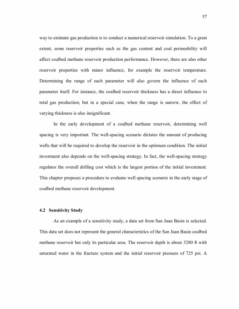
57
way to estimate gas production is to conduct a numerical reservoir simulation. To a great
extent, some reservoir properties such as the gas content and coal permeability will
affect coalbed methane reservoir production performance. However, there are also other
reservoir properties with minor influence, for example the reservoir temperature.
Determining the range of each parameter will also govern the influence of each
parameter itself. For instance, the coalbed reservoir thickness has a direct influence to
total gas production; but in a special case, when the range is narrow, the effect of
varying thickness is also insignificant.
In the early development of a coalbed methane reservoir, determining well
spacing is very important. The well-spacing scenario dictates the amount of producing
wells that will be required to develop the reservoir in the optimum condition. The initial
investment also depends on the well-spacing strategy. In fact, the well-spacing strategy
regulates the overall drilling cost which is the largest portion of the initial investment.
This chapter proposes a procedure to evaluate well spacing scenario in the early stage of
coalbed methane reservoir development.
4.2 Sensitivity Study
As an example of a sensitivity study, a data set from San Juan Basin is selected.
This data set does not represent the general characteristics of the San Juan Basin coalbed
methane reservoir but only its particular area. The reservoir depth is about 3280 ft with
saturated water in the fracture system and the initial reservoir pressure of 725 psi. A

58
dewatering stage is necessary in the early production stage. The following data set will
be a base case for further sensitivity study (Table 4.1).
A radial angular cylindrical grid is prepared to construct a single well, vertical
completion model. A reservoir is modeled by 31 x 1 grid size. In a single-well solution
and radial grid system, the finite-difference accuracy can be increased by using
geometrically spaced radial grids. This grid system provides a better solution for the
constant pressure or the constant rate boundary especially within the radius of up to a
half distance to the boundary. For the outer grid outside the first half distance to the
boundary, an equally-spaced grid can be used. The main purpose of using a
geometrically-spaced grid system is to get a better pressure profile near wellbore since
this area may have a faster pressure change. The well drainage radius is 1,053 ft or 80
acres well spacing.
A compositional simulator module from CMG (GEM) is used to perform a
numerical reservoir simulation for the base case data set. The simulation runs with a
constant pressure boundary of 14.7 psi at the bottom hole. The numerical simulation
model is shown in Fig. 4.1 while Fig. 4.2 shows the simulation result for the particular
base case.
A typical coalbed methane reservoir production performance occurs in the
simulation result. In the early stage, the dewatering process is obtained by producing
water at an initial rate of 93 bpd and it rapidly declines to less than 10 bpd in 5 years
production. The gas production rate culminates in the amount of 205,500 scfd after 640

59
days, which is followed by decline and behavior as found in a conventional reservoir.
After 20 years of production, the gas rate will be at 31,634 scfd.
To perform a sensitivity study, certain ranges of data sets are selected. The
ranges do not represent the general characteristics of the San Juan basin coalbed methane
reservoir. However, the data are taken form SPE papers with San Juan Basin as the
Parameter Value UnitThickness 30 ftFracture cleat spacing 0.042 ftFracture porosity 0.003Fracture permeability 1 mdFracture compressibility 100E-6 psi -1
Matrix porosity 0.005Matrix permeability 0.1 mdMatrix compressibility 100E-6 psi -1
Water density. 62.4 lb/ft 3
Water viscosity 0.607 cpWater compressibility 4E-06 cpCoal density 89.5841 lb/ft 3
Langmuir volume 0.23 gmole/lbmLangmuir pressure 725.189 psiDesorption time 10 DaysInitial pressure, Fracture 1109.54 psiInitial water saturation, Matrix 0.592Initial water saturation, Fracture 0.999Reservoir temperature 113 °FDepth 3280 ft
Table 4.1 - Dataset for base case
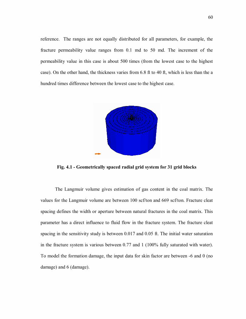
60
reference. The ranges are not equally distributed for all parameters, for example, the
fracture permeability value ranges from 0.1 md to 50 md. The increment of the
permeability value in this case is about 500 times (from the lowest case to the highest
case). On the other hand, the thickness varies from 6.8 ft to 40 ft, which is less than the a
hundred times difference between the lowest case to the highest case.
Fig. 4.1 - Geometrically spaced radial grid system for 31 grid blocks The Langmuir volume gives estimation of gas content in the coal matrix. The
values for the Langmuir volume are between 100 scf/ton and 669 scf/ton. Fracture cleat
spacing defines the width or aperture between natural fractures in the coal matrix. This
parameter has a direct influence to fluid flow in the fracture system. The fracture cleat
spacing in the sensitivity study is between 0.017 and 0.05 ft. The initial water saturation
in the fracture system is various between 0.77 and 1 (100% fully saturated with water).
To model the formation damage, the input data for skin factor are between -6 and 0 (no
damage) and 6 (damage).

61
Time (Date)
Gas
Rat
e SC
(ft3
/day
)
Wat
er R
ate
SC (b
bl/d
ay)
2005 2010 2015 20200.0e+0
5.0e+4
1.0e+5
1.5e+5
2.0e+5
2.5e+5
0
20
40
60
80
100
Gas Rate SC Water Rate SC
Fig. 4.2 - Reservoir simulation result of base case data set
After determining a particular range for each parameter, a sensitivity study is
then commenced. Table 4.2 shows the parameter range that has been used in the
sensitivity study. The main purpose of conducting a sensitivity study is to have a better
insight about the degree of the influence of each parameter. Hence, one can establish a
rank among all parameters and focus on improving measurement to obtain a more valid
value. For example, if the coal permeability really affects the production performance in
a great degree, an additional measurement technique should be performed in the initial

62
stage of coalbed methane reservoir development (e.g. by conducting whole core analysis
or pressure transient testing).
This work uses two methods to perform screening by sensitivity. The screening
should be conducted to all parameters to measure the influence of each parameter to the
production performance based on particular range. The first method is the One-Factor-
at-a-Time and the second is the Plackett-Burman method. For the base case and all other
cases, the well spacing is 80 acres. As a response of simulation result, this study uses
cumulative production after 20 years divided by the well spacing area, to obtain the
cumulative production per acre.
Parameter Min Base MaxThickness, ft 6.8 30 40Matrix porosity, fraction 0.0025 0.005 0.04Fracture porosity, fraction 0.0025 0.003 0.3Matrix permeability, md 0.01 0.1 1000Fracture permeability, md 0.1 1 50Fracture cleat spacing, ft 0.017 0.042 0.05
Matrix compressibility, 10-6 psi-1 10 100 200Fracture compressibility, 10-6 psi-1 10 100 200Water density. lb/ft 3 62.4 62.4 62.7Water compressibility, psi -1 2E-06 3E-06 4E-06Water viscosity, cp 0.550 0.607 0.730Reservoir temperature, °F 68 113 114Coal density, lb/ft 3 81.00 89.58 109Langmuir volume, gmole/lbm 0.06 0.23 0.4Reciprocal Langmuir pressure, psi -1 0.001 0.0014 0.0032Desorption time, Days 5 10 20Initial pressure, psi 339 1110 1422Initial water saturation, Fracture 0.77 0.999 1Initial water saturation, Matrix 0.1 0.592 1Skin -6 0 6
Table 4.2- Parameter range

63
As a methodology, the One-Factor-A-Time method is very common and it has
been widely used as a sensitivity study tool. For every number of parameters, each one
has 3 values: the minimum value, the most likely value, and the maximum value. A base
case is a result of all parameters in the most likely value. To obtain the influence of each
parameter, one can change the value from the most likely value to extreme value only
for one parameter at a time while keeping the other parameters in the same value (the
most likely value). The advantage of this method is its simplicity and tendency to avoid
mistakes during experiment or simulation. However, the relationship between different
parameters cannot be recognized. The basic assumption in performing the One-Factor-
A-Time method is independent probability condition. It means each parameter does not
influence the result of any other parameter whether it is in the minimum value or the
maximum one.
Fig. 4.3 shows the One-Factor-A-Time result for 20 factors. To determine the
effect of each parameter, 41 simulation runs including the base case have been
conducted. A detailed simulation result is available in Appendix B.
Based on the study result, the fracture permeability is found to be the most
influential factor. However, the fracture permeability range itself should be considered.
In the simulation result of this study, the difference between the minimum value to the
maximum value is 500 times. The fracture permeability has a strong relationship with
the production performance. The fluid flow from the cleat system can be described using
the Darcy’s flow evaluation. The fracture permeability is one factor in Darcy’s flow

64
0 2 4 6 8 10 12
Cumulative production per acre (MMSCF/ac)
Fracture permeabilityThickness
Langmuir volumeInitial pressure
Fracture porosityMatrix porosityWater viscosity
SkinCoal density
Reciprocal Langmuir pressureReservoir temperatureInitial water saturationMatrix compressibility
Desorption timeFracture compressibility
Water compressibilityMatrix permeability
Fracture cleat spacingWater density
Initial water saturation
Fig. 4.3 - One-Factor-A-Time sensitivity study result
64

65
equation that affects the production performance. Based on this sensitivity study result,
coal seam thickness is found to be the second most influential factor. Coal seam
thickness value ranges from 6.8 ft to 40 ft. For 67 times of coal seam thickness
increment, the cumulative gas production per acre increases from 1.855 MMSCF to
10.909 MMSCF. It means that cumulative gas production strongly depends on the coal
seam thickness.
Another factor that creates a big impact on gas production is the Langmuir
volume. The Langmuir volume provides an estimation of gas content in the coal matrix.
A higher Langmuir volume value will increase the gas production performance.
Another sensitivity study method is Plackett-Burman. This method is also
categorized as a “two-level factorial design”. The main difference between the One-
Factor-A-Time approach and the Plackett-Burman approach is that in the latter the
combinations of all factors are taken into consideration.
Since a “two-level factorial design” investigates all combinations of each
parameter, the relationships between factors are taken into account. A detailed
calculation result of this method is available in Appendix C. In addition to being known
as sensitivity study, Plackett-Burman is also recognized as a screening tool. A sensitivity
study result based on Plackett-Burman method is shown in Fig. 4.4.

66
4.3 Economic Model
In carrying out a well-spacing study, it is compulsory to establish an economic
model. The economic model needs an estimation of the initial cost, including the
operational expenses and capital expenses. The operational expenses comprise the
production well maintenance, work over activities (in the average cost per well per
month), compression and pumping costs, safety, monitoring and verification activities.
Table 4.3 shows assumptions of single-well economic parameters for the economic
calculation. The capital expenditures cover production wells (US$ per feet for drilling
and completion cost), work over (US$ per feet), pipeline installations (US$ per in-
miles), pumping and compression costs. The monthly revenue is calculated based on
estimated gas production per month and gas price. With an assumption of 1050
MMBTU/SCF, the gas price is 4 US$/MMSCF. The discount rate is assumed as 10%
and the production tax 4.6%.
Since reservoir properties vary based on each range, the outcomes of the
estimated production performance also vary. The production performances will be
different for each data set. A regression model is constructed from the sensitivity study
result. In this work, not all of parameters will be considered to have a significant effect
on the production performance. The main idea of this procedure is to obtain a good
regression result, and fewer variables tend to have a better regression result. In the One-
Factor-A-Time method, 3 factors are taken into account in the regression model (Table
4.4).

67
0 1 2 3 4 5 6 7 8 9
Cumulative Production per Acre (MMSCF/ac)
Fracture permeabilityThickness
Langmuir volumeInitial water saturation,
Initial pressureSkin
Fracture porosityWater compressibility
Initial water saturation, MatrixMatrix porosity
Matrix permeabilityMatrix compressibility
Fracture compressibilityDesorption time
Reservoir temperatureWater viscosity
Water densityCoal density
Reciprocal Langmuir pressureFracture cleat spacing
Fig. 4.4 – Plackett-Burman sensitivity study result
67

68
Parameter Value UnitGeneral DataDepth : 3280 ftGas Heating Value : 1050 MMBTU/SCFGas Price : 4 US $/MMBTU
0.004 US $/SCFPipeline Length : 1 in-mileCompression Power : 20 BHPPump Power : 20 BHPEconomic ParametersDiscount Rate : 10 %Production Taxes : 4.6 %Capital ExpendituresProduction Wells : 100 US $/ftWorkover : 100 US $/ftPipeline : 20 US $/in-mileCompression : 1500 US $/BHPPumping : 200 US $/BHPTotal Capex : 689,980 US $Operational ExpendituresProduction Wells : 100 US $/moWorkover : 10 US $/moCompression : 0.1 US $/McfPumping : 0.3 US $/tonSafety, Monitoring, Verification : 100 US $/well/yearTotal Opex : 1420 US $/year
Table 4.3 - Single well economic parameters
Parameter Notation Minimum Most Likely MaximumFracture permeability, md F5 0.1 1 50Thickness, ft F1 6.8 30 40Langmuir volume, gmole/lbm F3 0.06 0.23 0.4
Table 4.4 - Data set for one factor at a time regression model

69
By using the One-Factor-A-Time method, there are 7 simulation runs available to
build a regression model. One case for the base and the other 6 cases represent the
extreme values (maximum and minimum). To perform a regression model, this work
uses the EREGRESS[Eregress] software application. The Net Present Value (NPV) is
calculated from the cash flow in 20 years gas production. The selected regression
equation is as follows:
Based on the regression result, a graphical evaluation is presented in Fig. 4.5.
The regression result quality is shown by matching the result with the 45-degree line.
Fig. 4.5 shows the quality of the regression model compared to the simulation result.
Based on the regression software calculation, R2 is 0.997. In a statistical model the R2
value represents how well the equation can predict the future outcome of a model, in this
case, the reservoir simulation model. The regression model represents the reservoir
simulation result for all values within the range. This regression model is utilized to
perform a Monte Carlo simulation.
To conduct a Monte Carlo simulation, 10,000 random numbers are prepared.
After obtaining the Monte Carlo simulation result, a cumulative distribution function is
constructed. The main reason of providing the cumulative distribution function is to have
estimation about the economic value of each well-spacing scenario. Fig. 4.6 shows the
cumulative distribution function of the One-Factor-A-Time method for 80 acres well
spacing.
118970003379000027.4494211901613303000 FFFFNPV

70
-1.0E+06
-5.0E+05
0.0E+00
5.0E+05
1.0E+06
1.5E+06
2.0E+06
2.5E+06
3.0E+06
3.5E+06
4.0E+06
-1.0E+06 -5.0E+05 0.0E+00 5.0E+05 1.0E+06 1.5E+06 2.0E+06 2.5E+06 3.0E+06 3.5E+06 4.0E+06
Simulation Result, NPV (US$)
Reg
ress
ion
Res
ult,
NP
V (U
S$)
Fig. 4.5 - Regression model calibration for the One-Factor-A-Time method Another regression model is built based on a “three factorial” design. A “three
factorial” design has 3 values for each parameter. The values represent the extremities,
which are the maximum, minimum, and most likely values.
This work uses a “three factorial design” of the Box Behnken method. While the
Plackett-Burman method is mainly used as a screening tool to select the most influential
factors, the Box Behnken method can be utilized as a tool to develop the regression of
response from the simulation result.
Based on the screening result, the next sequence is to select the most important
parameter that will be used in the regression model. Instead of using the Plackett-
Burmann method, the Box Behnken method is chosen to conduct regression model. Both

71
0.E+00
1.E-07
2.E-07
3.E-07
4.E-07
5.E-07
6.E-07
7.E-07
-1.E+06 0.E+00 1.E+06 2.E+06 3.E+06 4.E+06 5.E+06
Net Present Value (US$)
Prob
abili
ty D
ensit
y Fu
nctio
n
0
0.1
0.2
0.3
0.4
0.5
0.6
0.7
0.8
0.9
1
Cum
ulat
ive
Dist
ribu
tion
Func
tion.
Probability Density Function
Cumulative Density Function
Fig. 4.6 - Probability density function and cumulative distribution function for the One-Factor-A-Time method
methods, the Plackett-Burman and Box Behnken, are condition-based probability. In
condition-based probability, there are relationships among the factors. A number of
simulation runs are designed based on the combinations among all factors in the
minimum, most likely, and maximum values.
Parameter Notation Minimum Most Likely MaximumFracture permeability, md F1 0.1 1 50Thickness, ft F2 6.8 30 40Langmuir volume, gmole/lbm F3 0.06 0.23 0.4
Table 4.5 - Data set for Box Behnken method

72
Table 4.5 shows the range of 3 selected parameters that have been used in the
Box Behnken method. This work used 16 simulation runs to provide regression model
data. A detailed explanation of this method and the simulation runs result is available in
Appendix E. The regression result for this method is:
Based on the regression result, a graphical evaluation is shown in Fig. 4.7. The more the
regression result matches with the 45-degree line, the better the regression result is.
The Net Present Value (NPV) is calculated from the cash flow in 20 years’ gas
production. Based on the selected regression model, this works used 10,000 random
numbers in performing the Monte Carlo simulation. The Monte Carlo simulation
provides the probability density function and cumulative density function of the Box
Behnken method (Fig. 4.8).
A comparison of the One-Factor-A-Time method and the Box Behnken method
is shown in Fig. 4.8. In this case, the Box Behnken method provides a more realistic
probability and cumulative density function with a wider range. The Net Present Value
range for the One-Factor-A-Time method is between US$ -931,970 and US$ 4,515,806.
On the other hand, the Box Behnken method gives a broader range from US$ -5,086,248
to US$ 6,897,093. This result illustrates the main difference between the One-Factor-A-
Time method and the Box Behnken method. The Box Behnken method, which is a
factorial design, considers the extreme condition when there is relationship among
factors.
31193907213.1999340100031735000
2259740118780003925300025.934513385458312673 FFFFeF
FFFFFNPVF
73
-1.0E+06
-5.0E+05
0.0E+00
5.0E+05
1.0E+06
1.5E+06
2.0E+06
2.5E+06
3.0E+06
3.5E+06
4.0E+06
-1.0E+06 -5.0E+05 0.0E+00 5.0E+05 1.0E+06 1.5E+06 2.0E+06 2.5E+06 3.0E+06 3.5E+06 4.0E+06
Simulation Result, NPV (US$)
Reg
ress
ion
Res
ult,
NPV
(US
$)
Fig. 4.7 - Regression model calibration for the Box Behnken method
Table 4.6 shows the Net Present Value comparison between the One-Factor-A-
Time approach and the Box Behnken approach based on the Monte Carlo simulation
result. The Monte Carlo simulation represents the uncertainty of the obtained Net
Present Value model from the regression result of the sensitivity One-Factor-A-Time
and Box Behnken methods. This work uses a triangle distribution to represent the
uncertainty of each parameter.
To give better explanation, it is common to present the Monte Carlo simulation
result with the following notations: P 10, P 50, and P 90. The meaning of the first
notation (P 10) is the possibility to acquire a value lower than P 10 value is 10%. In
other words, there is a possibility of 1 out of 10 that the outcome is lower than expected

74
value. The P 10 result is also known as the proved value. The same interpretation
applies for P 50 and P 90 notations. The P 50 value is also known as the probable value
and the P 90 as the possible value.
0.E+00
5.E-08
1.E-07
2.E-07
2.E-07
3.E-07
-6.E+06 -4.E+06 -2.E+06 0.E+00 2.E+06 4.E+06 6.E+06 8.E+06
Net Present Value (US$)
Prob
abili
ty D
ensit
y Fu
nctio
n
0
0.1
0.2
0.3
0.4
0.5
0.6
0.7
0.8
0.9
1
Cum
ulat
ive
Dist
ribu
tion
Func
tion.
Probability Density Function
Cumulative Density Function
Fig. 4.8 - Probability density function and cumulative distribution function for the Box Behnken method
Parameter One Factor at A Time Box BehnkenP 10 1,559,034 -826,566P 50 3,117,715 1,982,409P 90 3,897,188 4,441,489Minimum -931,970 -5,086,248Maximum 4,515,806 6,897,093
Table 4.6 - Net Present Value (US $)

75
The Monte Carlo simulation needs a distribution type for the input data or
parameters to present the uncertainty. The distribution type can be a normal distribution,
a log normal distribution, a rectangle distribution, or a triangle distribution. This work
uses a triangle distribution that can capture 3 values at a time: the minimum value, most-
likely value, and maximum value.
By using parameters in a certain distribution type, regression model, and random
number, one could yield a very different profile of distribution in the simulation result. A
graphical approach has been used in this work as distribution function. As shown in Fig.
4.9, the probability density function and cumulative distribution function of the Box
Behnken approach provide a wider Net Present Value range.
The Box Behnken method has been selected to perform the evaluation of well-
spacing effect on an economic model. To investigate the effect of well spacing, this
work has used the same data set and regression model. The similar work flow is applied
to all well spacing scenarios (Fig. 4.10). The first step is to establish the simulation
model. This step includes checking the consistency of the data set being used.
The following sequence is to identify the key responses from the simulation
model. The key responses are the expected result from the simulation model; it could be
a recovery factor, cumulative gas production, or original gas in place. Afterwards, the
next sequence is to identify parameters in the input data and the uncertainty ranges.
The next step is to run simulation using extreme cases to check the stability of
the simulation model in extreme conditions. The next step is to perform a parametric
study to screen the most influential factors that will be used in regression model. In this

76
step, a modification of range parameter is required in each case that yields an unstable
simulation result.
0.E+00
1.E-07
2.E-07
3.E-07
4.E-07
5.E-07
6.E-07
7.E-07
-6.E+06 -4.E+06 -2.E+06 0.E+00 2.E+06 4.E+06 6.E+06 8.E+06
Net Present Value (US$)
Prob
abili
ty D
ensit
y Fu
nctio
n
0
0.1
0.2
0.3
0.4
0.5
0.6
0.7
0.8
0.9
1
Cum
ulat
ive
Dist
ribu
tion
Func
tion.
PDF Box BehnkenPDF One Factor at a TimeCDF Box BehnkenCDF One Factor at a Time
Fig. 4.9 - Comparison of probability density function and cumulative distribution function
After selecting the most influential factors that will be used in the regression
model, then the regression model can be initiated. The regression model result needs to
be evaluated whether it is consistent with the reservoir simulation result. This step can be
done by using a graphical approach plotting regression model result and a simulation
model result. If the regression result is acceptable, the plot will tend to follow the 45-
degree tangent line.

77
When the regression result is not agreeable, a trial and error approach in building
the regression model is necessary. If the regression model is found satisfying, the next
step is to perform the Monte Carlo simulation. Before conducting the Monte Carlo
simulation, one should establish the distribution of the input parameter. This work has
used a triangle distribution to present uncertainty of response function. The response
function in this model is the Net Present Value per acre after having 20 years of
production.
As shown in Fig. 4.11, each well-spacing scenario alters the probability
distribution function and cumulative distribution function of the Net Present Value
(calculated per acre for 20 years’ production). A better economic model result tends to
shift the curve to the right. Following each pair of curves (the probability density
function and cumulative density function), the 320-acre well-spacing creates the lowest
Net Present Value distribution.
Furthermore, decreasing well-spacing seems to improve the Net Present Value
distribution. However, there is an optimum condition between 40 acres and 80 acres.
Increasing well-spacing to 320 acres tends to shift the Net Present Value distribution
function to the left as shown in Fig. 4.11. It means well-spacing scenarios bigger than 80
acres creates a lower Net Present Value distribution.

78
Establish reservoir simulation model
Identify key response from model, e.g. cumulative gas per acre after 20 years production
Identify parameters uncertainty and the uncertainty ranges
Run simulation at the extreme combination ofparameters to test ranges of each parameters
Perform parametric study
Identify most influential factors
Develop regression model
Test consistency of regression model
Acceptable regression model ?
Generate Monte Carlo simulation
Generate cumulative distribution function
Acceptable range ?
Fig. 4.10 – Well-spacing study work flow

79
0.E+00
5.E-06
1.E-05
2.E-05
2.E-05
3.E-05
3.E-05
4.E-05
4.E-05
5.E-05
5.E-05
-1.3E+05 -7.5E+04 -2.5E+04 2.5E+04 7.5E+04 1.3E+05
Net Present Value per acre (US$/ac)
Prob
abili
ty D
ensit
y Fu
nctio
n
0
0.1
0.2
0.3
0.4
0.5
0.6
0.7
0.8
0.9
1
Cum
ulat
ive
Dist
ribu
tion
Func
tion.PDF 320 ac
PDF 160 acPDF 80 acPDF 60 acPDF 40 acPDF 20 acCDF 320 acCDF 160 acCDF 80 acCDF 60 acCDF 40 acCDF 20 ac
Fig. 4.11 - Comparison of distribution function

80
CHAPTER V
CONCLUSIONS AND RECOMMENDATIONS
5.1 Conclusions
Based on the obtained results of this research, I offer the following conclusions:
1) To perform reservoir simulation, it is necessary to investigate the consistency of the
reservoir model result. In a special case, the combination of each parameter in a
coalbed methane reservoir model can yield inconsistency in the numerical model
result.
2) A parametric study is mandatory in evaluating the uncertainty of reservoir properties.
A parametric study gives illustration about the relationship among the parameters
and provides possible extreme conditions that should be considered in coalbed
methane reservoir modeling.
3) As a screening technique, the Placket-Burman method can be utilized to investigate
the influence of each parameter based on the various possible combinations with
other parameters.
4) A regression model needs a “three factorial design” to present the minimum, most
likely, and maximum condition of each parameter. The Box Behnken method
provides an approach to model the response of reservoir simulation results. This
method can be used in building a regression model to replace reservoir simulation
using the Monte Carlo simulation.

81
5) Investigation of well-pacing effect can be conducted using the Monte Carlo
simulation as a representative of the uncertainty in the reservoir properties.
5.2 Recommendations
The following recommendations are proposed to improve a well-spacing study in
a coalbed methane reservoir:
1. It is necessary to build an interface application between input data modification
(excel file) and reservoir simulator (CMG). By using this application one could
perform simulation runs without making data input for each case, and so a wider
parametric study can be done automatically. Another advantage of having this
application is that it can avoid human errors in finding the result of the simulation
run and in entering input data for the simulator.
2. It is necessary to continue a well-spacing study with different reservoir models. For
instance, researchers should investigate hydraulic fracturing and its effect on well-
spacing scenarios. The study can also include investigation of a hydraulic fracturing
model with different half-lengths and conductivities. The study can also be improved
by considering horizontal wells for a thin formation. Another variable in the
horizontal well model is the horizontal length. This variable should be incorporated
in the regression model.
3. The dewatering phase in a coalbed methane reservoir needs to be investigated. A
further study can be conducted based on aquifer modeling and its influence on well-
spacing study.

82
NOMENCLATURE
q = drainage rate per unit volume,
p = pressure, psia
B = formation volume factor, rb/stb
S = saturation, fraction
r = radius, ft
t = time, days
C = Coalbed gas content, Mscf/rcf
Fs = shape factor, 1/ft2
D = Diffusion coefficient, cm2/sec
Dc = diffusion coefficient, ft2/day
A = area, ft2
k = permeability, md
L = Length, ft
V(p) = gas content a pressure = p, scf/ton
VL = Langmuir volume, scf/ton
pL = Langmuir pressure, psia
Greek symbols
viscosity, cp
= porosity

83
= dimensionless storativity ratio
= shape factor, ft-2
= dimensionless interporosity flow parameter
τ = sorption time, days
Subscript
w = water
g = gas
m = matrix
f = fracture

84
REFERENCES
1. Annual Energy Outlook 2010, U.S. Energy Information Administration.
DOE/EIA-0383(2010). http://www.eia.doe.gov/oiaf/aeo/pdf/0383(2010).pdf
2. International Energy Outlook 2010, U.S. Energy Information Administration,
DOE/EIA-0484(2010). http://www.eia.doe.gov/oiaf/ieo/pdf/0484(2010).pdf
3. Ayers Jr., W. B. 2002. Coalbed Gas Systems, Resources, and Production and a
Review of Contrasting Cases from the San Juan and Powder River Basins. AAPG
Bulletin. 86: 1853-1890.
4. Ayers, W. B. Fall 2008. PETE 612 – Unconventional Reservoir Class Notes,
Texas A&M University.
5. Cook, T. 2005. Chapter 23: Calculation of Estimated Ultimate Recovery (EUR)
for Wells in Continuous Type Oil and Gas Accumulations. www.pubs.usgs.gov
/dds/dds-069/dds-069-d/REPORTS/69_D_CH_23.pdf
6. Wise, R.L. 1979. Methane Recovery and Utilization from Coalbeds. SPE-8357.
7. John, Mike, Paul, Andrew, Charles, et al.2003. Producing Natural Gas from
Coal. Oilfield Review, Autumn 2003: 8-31.
8. Warren, J.E., and Root, P.J. 1963. The Behavior of Naturally Fractured
Reservoirs. SPE-426..
9. Puri, R., and Yee, D. 1990. Enhanced Coalbed Methane Recovery. SPE-
20732.

85
10. Barenblatt, G.I., Zheltov, I. P., and Kochina, I.N. 1960. Basic Concepts in the
Theory of Seepage of Homogeneous Liquids in Fissured Rocks (Strata). PMM.
24 No 5: 852-864.
11. David, Turgay, Wonmo, and Gregory. 1984. A Parametric Study of the Effects of
Coal Seam Properties on Gas Drainage Efficiency. SPE-13366.
12. Olufemi, Turgai, Duane, Grant, Neal, et al. 2004. Carbon Dioxide Sequestration
in Coal Seams: A Parametric Study and Development of a Practical
Prediction/Screening Tool Using Neuro-Simulation. SPE-90055.
13. Cervik, J.1967. Behavior of Coal-Gas Reservoir. SPE-1973.
14. Zuber, M.D., Sawyer, W.K., Schraufnagel, R.A., and Kuuskaraa, V.A. 1987. The
Use of Simulation and History Matching to Determine Critical Coalbed Methane
Reservoir Properties. SPE-16420.
15. Seidle, J.P. and Arri, L.E. 1990. Use of Conventional Reservoir Models for
Coalbed Methane Simulation. SPE-21599.
16. King, G.R. 1990. Material Balance Techniques for Coal Seam and Devonian
Shale Gas Reservoirs. SPE-20730.
17. Seidle J.P. 1999. A Modified p/z Method for Coal Wells. SPE-55605.
18. David, H. and Law, S. 2002. Numerical Simulator Comparison Study for
Enhanced Coalbed Methane Recovery Processes, Part I: Carbon Dioxide
Injection. SPE-75669.
19. Hower, T.L.2003. Coalbed Methane Reservoir Simulation: An Evolving Science.
SPE-84424.

86
20. Jalal, J. and Shahab, D.M. 2004. A Coalbed Methane Reservoir Simulator
Designed for the Independent Producers. SPE-91414.
21. Aminian, K., Ameri, S., Bhavsar, A., Sanchez, M., and Garcia, A. Type Curves
for Coalbed Methane Production Prediction. SPE-91482.
22. Reeves, S. and Pekot, L. 2001. Advanced Reservoir Modeling in Desorption-
Controlled Reservoirs. SPE-71090.
23. Thomas, Tan. 2002. Advanced Large–Scale Coalbed Methane Modeling Using a
Conventional Reservoir Simulator. SPE-75672.
24. Paul, G.W., Sawyer, W.K., and Dean, R.H. 1990. Validation of 3D Coalbed
Simulators. SPE-20733.
25. Xiao Guo, Zhimin Du, and Shilun Li. 2003. Computer Modeling and Simulation
of Coalbed Methane Reservoir. SPE-84815.
26. Derickson, J.P., Horne, J.S., Fisher, R.D., and Stevens, S.H. 1998. Huabei
Coalbed Methane Project, Anhui Province, People's Republic of China. SPE-
48886.
27. Roadifer, R.D., Moore, T.R., Raterman, K.T., Farnan, R.A., and Crabtree, B.J.
Coalbed Methane Parametric Study: What's Really Important to Production and
When?. SPE-84425.
28. Stevenson, M.D., Pinczewski, W.V., and Downey, R.A. 1993. Economic
Evaluation of Nitrogen Injection for Coalseam Gas Recovery. SPE-26199.

87
29. Reeves, S.R. and Decker, A.D.1991. A Reservoir Simulation Investigation into
the Interaction of Is-Situ Stress, Pore Pressure, and Coal Rank on Coalbed
Methane Exploration Strategy. SPE-21490.
30. Young, G.B.C., McElhiney, J.E., Paul, G.W., and McBane, R.A. 1991. An
Analysis of Fruitland Coalbed Methane Production, Cedar Hill Field, Northern
San Juan Basin. SPE-22913.
31. Young, G.B.C., McElhiney, J.E., Paul, G.W., and McBane, R.A.1992. A
Parametric Analysis of Fruitland Coalbed Methane Producibility. SPE-24903.
32. Wicks, D.E., Schewerer, F. C., Militzer, M.R., and Zuber, M.D. 1986. Effective
Production Strategies for Coalbed Methane in the Warrior Basin. SPE-15234.
33. Chaianansutcharit, T. Her-Yuan Chen, and Teufel, L.W. 2001. Impacts of
Permeability Anisotropy and Pressure Interference on Coalbed Methane (CBM)
Production. SPE-71069..
34. King, G.R. 1990. Material-Balance Techniques for Coal Seam and Devonian
Shale Gas Reservoirs with Limited Water Influx. SPE-20730.
35. Jochen, V.A., Lee, W.J., and Semmelback, M.E. 1994. Determining Permeability
in Coalbed Methane Reservoirs. SPE-28584.
36. Reservoir Assesment Report Analysis Submitted to El Paso Production
Company, Ticora Geo., Arvada, Colorado, (August 2004).
37. Kohler, E.T. and Ertekin, Turgay. 1995. Modeling of Undersaturated Coal Seam
Gas Reservoirs. SPE-29578.

88
38. Bumb, A.C. and McKee, C.R. 1984. Use of a Computer Model to Design
Optimal Well for Dewatering Coal Seams for Methane Production. SPE-12859.
39. Sung, W., Ertekin, T., and Schewerer, F. C. 1987. An Analysis of Field
Development Strategies for Methane Production from Coal Seams. SPE-16858.
40. CMG; GEM 2003.10 User Guide, Computer Modeling Group Calgary, Canada.
41. Kamel Rekab and Muzaffar Shaikh. Statistical Design of Experiments with
Engineering Applications. CRC Press, 2005

89
APPENDIX A
CMG BASE CASE DATA FILE
*TITLE1 'CBM Case' *INUNIT *FIELD *INTERRUPT *INTERACTIVE *XDR *ON *OUTSRF *WELL *MAXERROR 20 *RANGECHECK ON *WRST 0 *WPRN *WELL 5 *WPRN *GRID *TIME *WSRF *WELL 5 *WSRF *GRID 1 *OUTPRN *WELL *ALL *OUTPRN *GRID *PRES *SW *SG *DENW *DENG *VISG *ADS 'C1' *Y 'C1' *OUTPRN *RES *ALL *OUTSRF *GRID *PRES *SW *SG *DENW *DENG *VISG *ADS 'C1' *Y 'C1' *OUTSRF *RES *ALL **--------------------------------------------------RESERVOIR DATA------ *GRID *RADIAL 31 1 1 *RW 1.5 *KDIR *DOWN *DI *IVAR 0.353 0.436 0.539 0.666 0.823 1.016 1.256 1.551 1.917 2.368 2.925 3.614 4.465 5.516 6.815 8.419 10.401 12.850 15.875 19.613 24.231 29.935 36.983 45.690 56.448 69.737 86.156 150.277 150.277 150.277 150.277 *DJ *CON 360 *DK *CON 30 *PAYDEPTH *ALL 31*3280

90
**--------------------------------------------DUAL POROSSITY OPTION----- *DUALPOR *NULL *MATRIX *CON 1. *NULL *FRACTURE *CON 1. *PINCHOUTARRAY *CON 1. **--------------------------------------------POROSITY DATA------------- *POR *MATRIX *CON 0.005 *POR *FRACTURE *CON 0.001 **--------------------------------------------PERMEABILITY DATA--------- *PERMI *MATRIX *CON 0.00001 *PERMI *FRACTURE *CON 1 *PERMJ *MATRIX *CON 0.00001 *PERMJ *FRACTURE *CON 1 *PERMK *MATRIX *CON 0.00001 *PERMK *FRACTURE *CON 1 **---------------------------------------FRACTURE SPACING DATA---------- *DIFRAC *CON 0.042 *DJFRAC *CON 0.042 *DKFRAC *CON 0.042 *---------------------------------------COMPRESSIBILITY DATA (MATRIX)-- *CPOR *MATRIX 100E-6 *PRPOR *MATRIX 1109.54 **-------------------------------------COMPRESSIBILITY DATA (FRACTURE)-- *CPOR *FRACTURE 100E-6 *PRPOR *FRACTURE 1109.54 **-------------------------------METHANE AND WATER DATA----------------- *MODEL *PR *NC 1 1 *COMPNAME 'C1' *HCFLAG 0 *VISCOR *HZYT *VISCOEFF 0.1023 0.023364 0.058533 -0.040758 0.0093324 *MIXVC 1 *TRES 113. **F *PCRIT 45.4 *TCRIT 190.6 *AC 0.008

91
*VCRIT 0.099 *MW 16.043 *PCHOR 77 *SG 0.3 *TB -258.61 *VISVC 0.099 *VSHIFT 0 *OMEGA 0.45723553 *OMEGB 0.077796074 *PVC3 1.2 *PHASEID *DEN *DENW 62.4 *CW 3.99896E-06 *REFPW 14.69595 *VISW 0.607 **======================= ROCK-FLUID PROPERTIES *ROCKFLUID ** GAS COAL NATURAL FRACTURE REL. PERM WATER-GAS *RPT 1 *SWT ** Sw Krw Krow ** ------- -------- -------- 0.00000 0.0000 1.0 1.00000 1.0000 0.0 *SGT ** Gas Sat Krg Krog ** ------- -------- -------- 0.0 0.0 1.0 1.0 1.0 0.0 ** Use the same relperm for matrix and fractures *RPT 2 *SWT ** Sw Krw Krow ** ------- -------- -------- 0.00000 0.0000 1.0 1.00000 1.0000 0.0 *SGT ** Gas Sat Krg Krog ** ------- -------- -------- 0.0 0.0 1.0 1.0 1.0 0.0 *RTYPE MATRIX CON 1 *RTYPE FRACTURE CON 2

92
**------------ SORPTION ISOTHERM DATA------------------ *ROCKDEN MATRIX CON 89.58 **(lb/ft3)** Matrix & fracture density, specific gravity * 62.428 *ROCKDEN FRACTURE CON 89.58 **(lb/ft3) ** NO SORPTION IN FRACTURE SYSTEM ** IN-SITU LANGMUIR STORAGE CAPACITY, gmole/lb *ADGMAXC 'C1' FRACTURE CON 0.0 ** RECIPROCAL LANGMUIR PRESSURE, 1/psi *ADGCSTC 'C1' FRACTURE CON 0.0 ** SORPTION IN MATRIX ** IN-SITU LANGMUIR STORAGE CAPACITY gmole / lbm ** g mole / lbm rock = 5.9760E-4 * scf/ton *ADGMAXC 'C1' MATRIX CON 0.23 ** RECIPROCAL LANGMUIR PRESSURE, 1/psi *ADGCSTC 'C1' MATRIX CON 0.0014 ** Coal Sorption times, Days *COAL-DIF-TIME 'C1' CON 10 **--------------------------------------------------INITIAL CONDITION------- *INITIAL *VERTICAL *BLOCK_CENTER *COMP *NREGIONS 2 REFPRES 1109.54 1109.54 REFDEPTH 3280 3280 DWOC 328 328 SWOC 0.9999 0.592 CDEPTH 3280 3280 ZDEPTH 1 3280 1 2 3280 1 *SEPARATOR 14.69595 59 *ITYPE *MATRIX *CON 2. *ITYPE *FRACTURE *CON 1. **--------------------------------------------------NUMERICAL DATA---------- *NUMERICAL DTMAX 30 CONVERGE PRESS 0.514884 *RUN

93
**-------------------------------------------------SIMULATION--------------- **START DATE *DATE 2000 01 01 ** **--------------------------------------------------WELL DATA--------------- ** *WELL 1 'PRODUCER 1' **$ WELL 'PRODUCER 1' **---------------------------------------------PRODUCTION CONSTRAINT-------- PRODUCER 'PRODUCER 1' OPERATE MIN BHP 14.7 CONT **$ rad geofac wfrac skin GEOMETRY K 0.25 0.37 1. 3. PERF GEO 'PRODUCER 1' **$ UBA ff Status Connection 1 1 1 1. OPEN FLOW-TO 'SURFACE' **$ RESULTS PROP AIMSET FRACTURE Units: Dimensionless **$ RESULTS PROP Minimum Value: 3 Maximum Value: 3 *AIMSET *FRACTURE *CON 3 **$ RESULTS PROP AIMSET MATRIX Units: Dimensionless **$ RESULTS PROP Minimum Value: 3 Maximum Value: 3 *AIMSET *MATRIX *CON 3 **---------------------------------------------TIME STEP-------------------- *TIME 1 *TIME 2 *TIME 10 *TIME 20 *TIME 30 cont. *TIME 7280 *TIME 7300 STOP **-------------------------------------------TERMINATE SIMULATION-----------

94
APPENDIX B
ONE-FACTOR-AT-A-TIME METHOD CALCULATION
Parameter Min Base Max NotationThickness, ft 6.8 30 40 F1Matrix porosity, fraction 0.0025 0.005 0.04 F2Fracture porosity, fraction 0.0025 0.003 0.3 F3Matrix permeability, md 0.01 0.1 1000 F4Fracture permeability, md 0.1 1 50 F5Fracture cleat spacing, ft 0.017 0.042 0.05 F6Matrix compressibility, 10-6 psi-1 10 100 200 F7Fracture compressibility, 10-6 psi-1 10 100 200 F8Water density. lb/ft 3 62.4 62.4 62.7 F9Water compressibility, psi -1 2E-06 3E-06 4E-06 F10Water viscosity, cp 0.550 0.607 0.730 F11Reservoir temperature, °F 68 113 114 F12Coal density, lb/ft 3 81.00 89.58 109 F13Langmuir volume, gmole/lbm 0.06 0.23 0.4 F14Reciprocal Langmuir pressure, psi -1 0.001 0.0014 0.0032 F15Desorption time, Days 5 10 20 F16Initial pressure, psi 339 1110 1422 F17Initial water saturation, Fracture 0.77 0.999 1 F18Initial water saturation, Matrix 0.1 0.592 1 F19Skin -6 0 6 F20
Table 4.2- Parameter range

95
1 2 3 4 5F1 30 6.8 40 30 30F2 0.005 0.005 0.005 0.0025 0.04F3 0.003 0.003 0.003 0.003 0.003F4 0.1 0.1 0.1 0.1 0.1F5 1 1 1 1 1F6 0.042 0.042 0.042 0.042 0.042F7 100 100 100 100 100F8 100 100 100 100 100F9 62.4 62.4 62.4 62.4 62.4F10 3E-06 3E-06 3E-06 3E-06 3E-06F11 0.607 0.607 0.607 0.607 0.607F12 113 113 113 113 113F13 89.5841 89.5841 89.5841 89.5841 89.5841F14 0.23 0.23 0.23 0.23 0.23F15 0.00138 0.00138 0.00138 0.00138 0.00138F16 10 10 10 10 10F17 1109.54 1109.54 1109.54 1109.54 1109.54F18 0.999 0.999 0.999 0.999 0.999F19 0.592 0.592 0.592 0.592 0.592F20 0 0 0 0 0Response, MMscf/acre 8.182 1.855 10.909 8.031 10.233
6 7 8 9 10F1 30 30 30 30 30F2 0.005 0.005 0.005 0.005 0.005F3 0.0025 0.3 0.003 0.003 0.003F4 0.1 0.1 0.01 1000 0.1F5 1 1 1 1 0.1F6 0.042 0.042 0.042 0.042 0.042F7 100 100 100 100 100F8 100 100 100 100 100F9 62.4 62.4 62.4 62.4 62.4F10 3E-06 3E-06 3E-06 3E-06 3E-06F11 0.607 0.607 0.607 0.607 0.607F12 113 113 113 113 113F13 89.5841 89.5841 89.5841 89.5841 89.5841F14 0.23 0.23 0.23 0.23 0.23F15 0.00138 0.00138 0.00138 0.00138 0.00138F16 10 10 10 10 10F17 1109.54 1109.54 1109.54 1109.54 1109.54F18 0.999 0.999 0.999 0.999 0.999F19 0.592 0.592 0.592 0.592 0.592F20 0 0 0 0 0Response, MMscf/acre 8.296 0.837 8.182 8.182 1.662
Simulation Run
Para
met
erPa
ram
eter
Table B.2 - One factor at a time simulation resultSimulation Run

96
11 12 13 14 15F1 30 30 30 30 30F2 0.005 0.005 0.005 0.005 0.005F3 0.003 0.003 0.003 0.003 0.003F4 0.1 0.1 0.1 0.1 0.1F5 50 1 1 1 1F6 0.042 0.017 0.05 0.042 0.042F7 100 100 100 10 200F8 100 100 100 100 100F9 62.4 62.4 62.4 62.4 62.4F10 3E-06 3E-06 3E-06 3E-06 3E-06F11 0.607 0.607 0.607 0.607 0.607F12 113 113 113 113 113F13 89.5841 89.5841 89.5841 89.5841 89.5841F14 0.23 0.23 0.23 0.23 0.23F15 0.00138 0.00138 0.00138 0.00138 0.00138F16 10 10 10 10 10F17 1109.54 1109.54 1109.54 1109.54 1109.54F18 0.999 0.999 0.999 0.999 0.999F19 0.592 0.592 0.592 0.592 0.592F20 0 0 0 0 0Response, MMscf/acre 13.500 8.182 8.182 8.175 8.190
16 17 18 19 20F1 30 30 30 30 30F2 0.005 0.005 0.005 0.005 0.005F3 0.003 0.003 0.003 0.003 0.003F4 0.1 0.1 0.1 0.1 0.1F5 1 1 1 1 1F6 0.042 0.042 0.042 0.042 0.042F7 100 100 100 100 100F8 10 200 100 100 100F9 62.4 62.4 62.4 62.712 62.4F10 3E-06 3E-06 3E-06 3E-06 2E-06F11 0.607 0.607 0.607 0.607 0.607F12 113 113 113 113 113F13 89.5841 89.5841 89.5841 89.5841 89.5841F14 0.23 0.23 0.23 0.23 0.23F15 0.00138 0.00138 0.00138 0.00138 0.00138F16 10 10 10 10 10F17 1109.54 1109.54 1109.54 1109.54 1109.54F18 0.999 0.999 0.999 0.999 0.999F19 0.592 0.592 0.592 0.592 0.592F20 0 0 0 0 0Response, MMscf/acre 8.182 8.183 8.182 8.182 8.182
Para
met
er
Simulation Run
Para
met
er
Simulation Run
Table B.2 - One factor at a time simulation result

97
21 22 23 24 25F1 30 30 30 30 30F2 0.005 0.005 0.005 0.005 0.005F3 0.003 0.003 0.003 0.003 0.003F4 0.1 0.1 0.1 0.1 0.1F5 1 1 1 1 1F6 0.042 0.042 0.042 0.042 0.042F7 100 100 100 100 100F8 100 100 100 100 100F9 62.4 62.4 62.4 62.4 62.4F10 4E-06 3E-06 3E-06 3E-06 3E-06F11 0.607 0.55 0.73 0.607 0.607F12 113 113 113 68 114F13 89.5841 89.5841 89.5841 89.5841 89.5841F14 0.23 0.23 0.23 0.23 0.23F15 0.00138 0.00138 0.00138 0.00138 0.00138F16 10 10 10 10 10F17 1109.54 1109.54 1109.54 1109.54 1109.54F18 0.999 0.999 0.999 0.999 0.999F19 0.592 0.592 0.592 0.592 0.592F20 0 0 0 0 0Response, MMscf/acre 8.182 8.238 8.067 8.579 8.174
26 27 28 29 30F1 30 30 30 30 30F2 0.005 0.005 0.005 0.005 0.005F3 0.003 0.003 0.003 0.003 0.003F4 0.1 0.1 0.1 0.1 0.1F5 1 1 1 1 1F6 0.042 0.042 0.042 0.042 0.042F7 100 100 100 100 100F8 100 100 100 100 100F9 62.4 62.4 62.4 62.4 62.4F10 3E-06 3E-06 3E-06 3E-06 3E-06F11 0.607 0.607 0.607 0.607 0.607F12 113 113 113 113 113F13 81 109 89.5841 89.5841 89.5841F14 0.23 0.23 0.06 0.4 0.23F15 0.00138 0.00138 0.00138 0.00138 0.001F16 10 10 10 10 10F17 1109.54 1109.54 1109.54 1109.54 1109.54F18 0.999 0.999 0.999 0.999 0.999F19 0.592 0.592 0.592 0.592 0.592F20 0 0 0 0 0Response, MMscf/acre 7.629 9.356 3.111 11.840 7.897
Simulation Run
Para
met
er
Table B.2 - One factor at a time simulation result
Simulation Run
Para
met
er

98
31 32 33 34 35F1 30 30 30 30 30F2 0.005 0.005 0.005 0.005 0.005F3 0.003 0.003 0.003 0.003 0.003F4 0.1 0.1 0.1 0.1 0.1F5 1 1 1 1 1F6 0.042 0.042 0.042 0.042 0.042F7 100 100 100 100 100F8 100 100 100 100 100F9 62.4 62.4 62.4 62.4 62.4F10 3E-06 3E-06 3E-06 3E-06 3E-06F11 0.607 0.607 0.607 0.607 0.607F12 113 113 113 113 113F13 89.5841 89.5841 89.5841 89.5841 89.5841F14 0.23 0.23 0.23 0.23 0.23F15 0.0032 0.00138 0.00138 0.00138 0.00138F16 10 5 20 10 10F17 1109.54 1109.54 1109.54 339 1422F18 0.999 0.999 0.999 0.999 0.999F19 0.592 0.592 0.592 0.592 0.592F20 0 0 0 0 0Response, MMscf/acre 7.658 8.187 8.172 2.166 9.619
36 37 38 39 40 41F1 30 30 30 30 30 30F2 0.005 0.005 0.005 0.005 0.005 0.005F3 0.003 0.003 0.003 0.003 0.003 0.003F4 0.1 0.1 0.1 0.1 0.1 0.1F5 1 1 1 1 1 1F6 0.042 0.042 0.042 0.042 0.042 0.042F7 100 100 100 100 100 100F8 100 100 100 100 100 100F9 62.4 62.4 62.4 62.4 62.4 62.4F10 3E-06 3E-06 3E-06 3E-06 3E-06 3E-06F11 0.607 0.607 0.607 0.607 0.607 0.607F12 113 113 113 113 113 113F13 89.5841 89.5841 89.5841 89.5841 89.5841 89.5841F14 0.23 0.23 0.23 0.23 0.23 0.23F15 0.00138 0.00138 0.00138 0.00138 0.00138 0.00138F16 10 10 10 10 10 10F17 1109.54 1109.54 1109.54 1109.54 1109.54 1109.54F18 0.77 1 0.999 0.999 0.999 0.999F19 0.592 0.592 0.1 1 0.592 0.592F20 0 0 0 0 0 6Response, MMscf/acre 8.351 8.182 8.182 8.182 8.182 6.692
Para
met
erPa
ram
eter
Simulation Run
Table B.2 - One factor at a time simulation resultSimulation Run

99
Parameter ResponseFracture permeability, md 11.8383Thickness, ft 9.0546Langmuir volume, gmole/lbm 8.7288Initial pressure, psi 7.8728Fracture porosity, fraction 7.4588Matrix porosity, fraction 2.2023Water viscosity, cp 1.7273Skin 1.4900Coal density, lb/ft 3 0.4055Reciprocal Langmuir pressure, psi-1 0.2391Reservoir temperature, °F 0.1704Initial water saturation, Fracture 0.1694Matrix compressibility, 10-6, psi -1 0.0153Desorption time, Days 0.0148Fracture compressibility, 10-6, psi -1 0.0014Water compressibility, psi -1 0.0008Matrix permeability, md 0.0000Fracture cleat spacing, ft 0.0000Water density. lb/ft 3 0.0000Initial water saturation, Matrix 0.0000
Table B.3 - Main effect result

100
APPENDIX C
SIMULATION RESULTS FOR PLACKETT-BURMAN METHOD
1 2 3 4 5 6 7 8 9 10 11 12 13 14F1 -1 -1 1 1 -1 1 1 -1 1 1 -1 -1 1 1F2 -1 1 1 -1 1 -1 -1 -1 -1 1 -1 1 -1 1F3 1 1 1 -1 -1 1 -1 1 1 -1 -1 1 1 1F4 -1 1 1 -1 1 -1 1 1 1 1 -1 -1 -1 1F5 1 1 1 -1 1 1 1 -1 1 -1 -1 -1 -1 -1F6 -1 1 -1 1 1 1 -1 -1 1 1 -1 1 1 -1F7 -1 -1 -1 -1 1 1 1 1 1 1 -1 1 1 -1F8 1 -1 -1 1 1 1 -1 1 -1 1 -1 -1 -1 -1F9 1 -1 -1 -1 -1 1 1 -1 -1 1 -1 1 -1 1F10 -1 -1 1 -1 -1 -1 1 1 -1 1 -1 -1 1 -1F11 -1 1 -1 1 -1 -1 1 -1 -1 -1 -1 1 1 1F12 1 -1 1 1 -1 -1 1 1 1 -1 -1 1 -1 -1F13 1 1 -1 -1 1 -1 1 1 -1 -1 -1 1 1 -1F14 -1 -1 -1 -1 -1 1 -1 1 1 -1 -1 1 -1 1F15 1 -1 1 1 1 -1 -1 1 -1 1 -1 1 1 1F16 -1 1 1 1 -1 1 -1 1 -1 -1 -1 -1 1 -1F17 1 1 -1 -1 -1 -1 -1 -1 1 1 -1 -1 1 -1F18 1 -1 -1 1 1 -1 1 -1 1 -1 -1 -1 1 1F19 1 -1 1 -1 1 1 -1 -1 -1 -1 -1 -1 1 1F20 1 1 1 1 -1 1 1 -1 -1 1 -1 1 -1 -1
Para
met
er
Table C.1 - Plackett-Burman simulation designSimulation Run
100

101
15 16 17 18 19 20 21 22 23 24 25F1 0 -1 -1 1 1 -1 1 -1 1 -1 -1F2 0 1 -1 1 1 -1 -1 1 1 -1 1F3 0 1 -1 -1 1 -1 -1 -1 -1 1 -1F4 0 -1 -1 -1 -1 1 1 1 -1 1 -1F5 0 1 1 -1 -1 -1 1 -1 1 -1 1F6 0 -1 -1 -1 -1 1 -1 -1 1 1 1F7 0 1 1 1 -1 -1 -1 1 -1 -1 -1F8 0 1 -1 -1 1 -1 1 1 1 1 -1F9 0 1 -1 1 -1 1 1 -1 -1 1 1F10 0 1 1 -1 1 1 -1 -1 1 1 1F11 0 1 1 -1 -1 -1 1 1 1 1 -1F12 0 -1 -1 1 -1 -1 -1 1 1 1 1F13 0 -1 -1 1 1 1 1 -1 1 -1 -1F14 0 -1 1 -1 1 1 1 1 1 -1 1F15 0 -1 1 -1 -1 -1 1 -1 -1 -1 1F16 0 1 -1 1 -1 1 1 1 -1 -1 1F17 0 -1 1 1 1 -1 1 1 -1 1 1F18 0 1 -1 -1 1 1 -1 1 -1 -1 1F19 0 -1 1 1 -1 1 -1 1 1 1 -1F20 0 -1 1 -1 1 1 -1 1 -1 -1 -1
Para
met
er
Simulation RunTable C.1 - Plackett-Burman simulation design
101

102
1 2 3 4 5 6 7 8 9 10 11 12 13 14F1 6.8 6.8 40 40 6.8 40 40 6.8 40 40 6.8 6.8 40 40F2 0.0025 0.04 0.04 0.0025 0.04 0.0025 0.0025 0.0025 0.0025 0.04 0.0025 0.04 0.0025 0.04F3 0.3 0.3 0.3 0.0025 0.0025 0.3 0.0025 0.3 0.3 0.0025 0.0025 0.3 0.3 0.3F4 0.01 1000 1000 0.01 1000 0.01 1000 1000 1000 1000 0.01 0.01 0.01 1000F5 50 50 50 0.1 50 50 50 0.1 50 0.1 0.1 0.1 0.1 0.1F6 0.017 0.05 0.017 0.05 0.05 0.05 0.017 0.017 0.05 0.05 0.017 0.05 0.05 0.017F7 10 10 10 10 200 200 200 200 200 200 10 200 200 10F8 200 10 10 200 200 200 10 200 10 200 10 10 10 10F9 62.712 62.4 62.4 62.4 62.4 62.712 62.712 62.4 62.4 62.712 62.4 62.712 62.4 62.712F10 2E-06 2E-06 4E-06 2E-06 2E-06 2E-06 4E-06 4E-06 2E-06 4E-06 2E-06 2E-06 4E-06 2E-06F11 0.55 0.73 0.55 0.73 0.55 0.55 0.73 0.55 0.55 0.55 0.55 0.73 0.73 0.73F12 114 68 114 114 68 68 114 114 114 68 68 114 68 68F13 109 109 81 81 109 81 109 109 81 81 81 109 109 81F14 0.06 0.06 0.06 0.06 0.06 0.4 0.06 0.4 0.4 0.06 0.06 0.4 0.06 0.4F15 0.0032 0.001 0.0032 0.0032 0.0032 0.001 0.001 0.0032 0.001 0.0032 0.001 0.0032 0.0032 0.0032F16 5 20 20 20 5 20 5 20 5 5 5 5 20 5F17 1422 1422 339 339 339 339 339 339 1422 1422 339 339 1422 339F18 1 0.77 0.77 1 1 0.77 1 0.77 1 0.77 0.77 0.77 1 1F19 1 0.1 1 0.1 1 1 0.1 0.1 0.1 0.1 0.1 0.1 1 1F20 6 6 6 6 0 6 6 0 0 6 0 6 0 0Response, MMscf/acre 0.78293 3.88125 5.1965 0.07494 0.94484 9.128 2.3255 0.04584 18.2913 3.46163 0.05351 0.02495 0.02914 0.05078
Table C.2 - Plackett-Burman simulation resultsSimulation Run
Para
met
er
102

103
15 16 17 18 19 20 21 22 23 24 25F1 30 6.8 6.8 40 40 6.8 40 6.8 40 6.8 6.8F2 0.005 0.04 0.0025 0.04 0.04 0.0025 0.0025 0.04 0.04 0.0025 0.04F3 0.003 0.3 0.0025 0.0025 0.3 0.0025 0.0025 0.0025 0.0025 0.3 0.0025F4 0.1 0.01 0.01 0.01 0.01 1000 1000 1000 0.01 1000 0.01F5 1 50 50 0.1 0.1 0.1 50 0.1 50 0.1 50F6 0.042 0.017 0.017 0.017 0.017 0.05 0.017 0.017 0.05 0.05 0.05F7 100 200 200 200 10 10 10 200 10 10 10F8 100 200 10 10 200 10 200 200 200 200 10F9 62.4 62.712 62.4 62.712 62.4 62.712 62.712 62.4 62.4 62.712 62.712F10 3E-06 4E-06 4E-06 2E-06 4E-06 4E-06 2E-06 2E-06 4E-06 4E-06 4E-06F11 0.607 0.73 0.73 0.55 0.55 0.55 0.73 0.73 0.73 0.73 0.55F12 113 68 68 114 68 68 68 114 114 114 114F13 89.5841 81 81 109 109 109 109 81 109 81 81F14 0.23 0.06 0.4 0.06 0.4 0.4 0.4 0.4 0.4 0.06 0.4F15 0.00138 0.001 0.0032 0.001 0.001 0.001 0.0032 0.001 0.001 0.001 0.0032F16 10 20 5 20 5 20 20 20 5 5 20F17 1109.54 339 1422 1422 1422 339 1422 1422 339 1422 1422F18 0.999 1 0.77 0.77 0.77 1 0.77 1 0.77 0.77 1F19 0.592 0.1 1 1 1 1 0.1 1 1 1 0.1F20 0 0 6 0 6 6 0 6 0 0 0Response, MMscf/acre 8.182 0.33366 5.72413 4.78875 2.54463 0.03279 45.9888 0.35569 14.9163 0.54635 6.73713
Para
met
erSimulation Run
Table C.2 - Plackett-Burman simulation results
103

104
APPENDIX D
ECONOMIC MODEL CALCULATION RESULTS FOR ONE-
FACTOR-AT-A-TIME METHOD
Simulation RunParameter
F1 1 0.1 50 1 1 1 1F2 30 30 30 6.8 40 30 30F3 0.23 0.23 0.23 0.23 0.23 0.06 0.4
Table D.1- One factor at a time simulation runs design
1 2 3 4 5 6 7
NPV(US $) Frequency Relative Frequency Probability Density Function Cumulative Distribution Function(931,970) 0 0 0.000E+00 0.000E+00(645,245) 6 0.0006 2.098E-09 3.008E-04(358,520) 15 0.0015 5.246E-09 1.354E-03
(71,795) 46 0.0046 1.609E-08 4.412E-03214,930 76 0.0076 2.658E-08 1.053E-02501,655 107 0.0107 3.742E-08 1.970E-02788,380 209 0.0209 7.309E-08 3.555E-02
1,075,105 217 0.0217 7.589E-08 5.690E-021,361,830 243 0.0243 8.498E-08 7.997E-021,648,555 338 0.0338 1.182E-07 1.091E-011,935,281 410 0.041 1.434E-07 1.466E-012,222,006 517 0.0517 1.808E-07 1.931E-012,508,731 761 0.0761 2.661E-07 2.571E-012,795,456 1112 0.1112 3.889E-07 3.510E-013,082,181 1467 0.1467 5.130E-07 4.803E-013,368,906 1696 0.1696 5.931E-07 6.389E-013,655,631 1492 0.1492 5.218E-07 7.988E-013,942,356 905 0.0905 3.165E-07 9.189E-014,229,081 329 0.0329 1.151E-07 9.808E-014,515,806 54 0.0054 1.888E-08 1.000E+00
Table D.2 - Monte Carlo simulation result, one factor at a time method

105
APPENDIX E
ECONOMIC MODEL CALCULATION RESULTS FOR BOX
BEHNKEN METHOD
Simulation RunsParameter
F1 0 1 0 -1 -1 -1 0 1F2 1 0 -1 0 0 -1 0 0F3 -1 -1 -1 1 -1 0 0 1
Simulation RunsParameter
F1 -1 0 0 0 0 1 0 1F2 1 0 1 -1 0 -1 0 1F3 0 0 1 1 0 0 0 0
13 14 15 169 10 11 12
1 2 3 4 5 6 7 8
Table E.1 - Box Behnken simulation design
Simulation RunsParameter
F1 1 50 1 0.1 0.1 0.1 1 50F2 40 30 6.8 30 30 6.8 30 30F3 0.06 0.06 0.06 0.4 0.06 0.23 0.23 0.4
Simulation RunsParameter
F1 1 50 1 0.1 0.1 0.1 1 50F2 40 30 6.8 30 30 6.8 30 30F3 0.06 0.06 0.06 0.4 0.06 0.23 0.23 0.4
Table E.2 - Box Behnken simulation data
9 10 11 12 13 14 15 16
1 2 3 4 5 6 7 8

106
NPV(US $) Frequency Relative Frequency Probability Density Function Cumulative Distribution Function(5,086,248) 1 0.0001 1.586E-10 0.000E+00(4,455,546) 12 0.0012 1.903E-09 6.503E-04(3,824,844) 31 0.0031 4.917E-09 2.801E-03(3,194,142) 85 0.0085 1.348E-08 8.604E-03(2,563,439) 139 0.0139 2.205E-08 1.981E-02(1,932,737) 232 0.0232 3.680E-08 3.837E-02(1,302,035) 348 0.0348 5.520E-08 6.738E-02
(671,333) 517 0.0517 8.201E-08 1.106E-01(40,631) 687 0.0687 1.090E-07 1.709E-01590,071 960 0.096 1.523E-07 2.533E-01
1,220,774 1149 0.1149 1.823E-07 3.588E-011,851,476 1180 0.118 1.872E-07 4.753E-012,482,178 1202 0.1202 1.907E-07 5.944E-013,112,880 1071 0.1071 1.699E-07 7.081E-013,743,582 959 0.0959 1.521E-07 8.097E-014,374,284 725 0.0725 1.150E-07 8.939E-015,004,987 419 0.0419 6.646E-08 9.511E-015,635,689 219 0.0219 3.474E-08 9.830E-016,266,391 56 0.0056 8.883E-09 9.968E-016,897,093 8 0.0008 1.269E-09 1.000E+00
Table E.3 - Monte Carlo simulation result, Box Behnken method

107
APPENDIX F
ECONOMIC MODEL CALCULATION RESULTS FOR WELL SPACING STUDY
NPV(US $) Frequency Relative Frequency Probability Density Function Cumulative Distribution Function(160,000) 0 0 0.000E+00 0.000E+00(145,789) 2 0.0002 1.408E-08 1.000E-04(131,579) 4 0.0004 2.816E-08 4.001E-04(117,368) 42 0.0042 2.956E-07 2.701E-03(103,158) 59 0.0059 4.153E-07 7.752E-03
(88,947) 161 0.0161 1.133E-06 1.876E-02(74,737) 183 0.0183 1.288E-06 3.596E-02(60,526) 356 0.0356 2.506E-06 6.292E-02(46,316) 449 0.0449 3.161E-06 1.032E-01(32,105) 622 0.0622 4.378E-06 1.567E-01(17,895) 797 0.0797 5.610E-06 2.277E-01(3,684) 1063 0.1063 7.483E-06 3.207E-0110,526 1420 0.142 9.996E-06 4.449E-0124,737 1513 0.1513 1.065E-05 5.916E-0138,947 1343 0.1343 9.454E-06 7.345E-0153,158 988 0.0988 6.955E-06 8.511E-0167,368 645 0.0645 4.540E-06 9.327E-0181,579 245 0.0245 1.725E-06 9.772E-0195,789 102 0.0102 7.180E-07 9.946E-01
110,000 6 0.0006 4.223E-08 1.000E+00
Table F.1 - Monte Carlo simulation results, 20 acres well spacing

108
NPV(US $) Frequency Relative Frequency Probability Density Function Cumulative Distribution Function(110,000) 0 0 0.000E+00 0.000E+00
(98,421) 4 0.0004 3.455E-08 2.000E-04(86,842) 21 0.0021 1.814E-07 1.450E-03(75,263) 43 0.0043 3.714E-07 4.650E-03(63,684) 110 0.011 9.500E-07 1.230E-02(52,105) 206 0.0206 1.779E-06 2.810E-02(40,526) 335 0.0335 2.893E-06 5.515E-02(28,947) 435 0.0435 3.757E-06 9.365E-02(17,368) 617 0.0617 5.329E-06 1.463E-01(5,789) 818 0.0818 7.065E-06 2.180E-015,789 1188 0.1188 1.026E-05 3.183E-01
17,368 1266 0.1266 1.093E-05 4.410E-0128,947 1339 0.1339 1.156E-05 5.713E-0140,526 1310 0.131 1.131E-05 7.037E-0152,105 1021 0.1021 8.818E-06 8.203E-0163,684 722 0.0722 6.236E-06 9.074E-0175,263 391 0.0391 3.377E-06 9.631E-0186,842 147 0.0147 1.270E-06 9.900E-0198,421 26 0.0026 2.246E-07 9.986E-01
110,000 1 0.0001 8.637E-09 1.000E+00
Table F.2 - Monte Carlo simulation results, 40 acres well spacing
NPV(US $) Frequency Relative Frequency Probability Density Function Cumulative Distribution Function(80,000) 0 0 0.000E+00 0.000E+00(70,526) 4 0.0004 4.222E-08 2.000E-04(61,053) 36 0.0036 3.800E-07 2.200E-03(51,579) 85 0.0085 8.973E-07 8.250E-03(42,105) 122 0.0122 1.288E-06 1.860E-02(32,632) 234 0.0234 2.470E-06 3.640E-02(23,158) 324 0.0324 3.420E-06 6.430E-02(13,684) 504 0.0504 5.320E-06 1.057E-01(4,211) 702 0.0702 7.410E-06 1.660E-015,263 937 0.0937 9.891E-06 2.480E-01
14,737 1159 0.1159 1.223E-05 3.528E-0124,211 1305 0.1305 1.378E-05 4.760E-0133,684 1317 0.1317 1.390E-05 6.071E-0143,158 1215 0.1215 1.283E-05 7.337E-0152,632 943 0.0943 9.954E-06 8.416E-0162,105 619 0.0619 6.534E-06 9.197E-0171,579 344 0.0344 3.631E-06 9.678E-0181,053 119 0.0119 1.256E-06 9.910E-0190,526 30 0.003 3.167E-07 9.984E-01
100,000 1 0.0001 1.056E-08 1.000E+00
Table F.3 - Monte Carlo simulation results, 60 acres well spacing

109
NPV(US $) Frequency Relative Frequency Probability Density Function Cumulative Distribution Function(70,000) 0 0 0.000E+00 0.000E+00(61,579) 1 0.0001 1.188E-08 5.001E-05(53,158) 17 0.0017 2.019E-07 9.501E-04(44,737) 56 0.0056 6.651E-07 4.600E-03(36,316) 119 0.0119 1.413E-06 1.335E-02(27,895) 218 0.0218 2.589E-06 3.020E-02(19,474) 309 0.0309 3.670E-06 5.656E-02(11,053) 483 0.0483 5.736E-06 9.616E-02(2,632) 652 0.0652 7.743E-06 1.529E-015,789 946 0.0946 1.123E-05 2.328E-01
14,211 1126 0.1126 1.337E-05 3.364E-0122,632 1249 0.1249 1.483E-05 4.552E-0131,053 1274 0.1274 1.513E-05 5.814E-0139,474 1227 0.1227 1.457E-05 7.064E-0147,895 1038 0.1038 1.233E-05 8.197E-0156,316 712 0.0712 8.456E-06 9.072E-0164,737 387 0.0387 4.596E-06 9.621E-0173,158 153 0.0153 1.817E-06 9.891E-0181,579 31 0.0031 3.682E-07 9.983E-0190,000 2 0.0002 2.375E-08 1.000E+00
Table F.4 - Monte Carlo simulation results, 80 acres well spacing
NPV(US $) Frequency Relative Frequency Probability Density Function Cumulative Distribution Function(29,000) 0 0 0.000E+00 0.000E+00(23,684) 14 0.0014 2.634E-07 7.001E-04(18,368) 60 0.006 1.129E-06 4.400E-03(13,053) 170 0.017 3.198E-06 1.590E-02(7,737) 285 0.0285 5.362E-06 3.865E-02(2,421) 444 0.0444 8.353E-06 7.511E-022,895 712 0.0712 1.340E-05 1.329E-018,211 1003 0.1003 1.887E-05 2.187E-01
13,526 1116 0.1116 2.100E-05 3.246E-0118,842 1172 0.1172 2.205E-05 4.390E-0124,158 1120 0.112 2.107E-05 5.537E-0129,474 1098 0.1098 2.066E-05 6.646E-0134,789 959 0.0959 1.804E-05 7.674E-0140,105 732 0.0732 1.377E-05 8.520E-0145,421 539 0.0539 1.014E-05 9.155E-0150,737 355 0.0355 6.679E-06 9.602E-0156,053 145 0.0145 2.728E-06 9.852E-0161,368 60 0.006 1.129E-06 9.955E-0166,684 14 0.0014 2.634E-07 9.992E-0172,000 2 0.0002 3.763E-08 1.000E+00
Table F.5 - Monte Carlo simulation results, 160 acres well spacing

110
NPV(US $) Frequency Relative Frequency Probability Density Function Cumulative Distribution Function(12,000) 0 0 0.000E+00 0.000E+00(9,474) 16 0.0016 6.334E-07 8.001E-04(6,947) 69 0.0069 2.732E-06 5.051E-03(4,421) 210 0.021 8.313E-06 1.900E-02(1,895) 327 0.0327 1.295E-05 4.585E-02
632 649 0.0649 2.569E-05 9.466E-023,158 837 0.0837 3.313E-05 1.690E-015,684 1027 0.1027 4.066E-05 2.622E-018,211 1081 0.1081 4.279E-05 3.676E-01
10,737 1130 0.113 4.473E-05 4.781E-0113,263 1111 0.1111 4.398E-05 5.902E-0115,789 1039 0.1039 4.113E-05 6.977E-0118,316 862 0.0862 3.412E-05 7.928E-0120,842 697 0.0697 2.759E-05 8.707E-0123,368 471 0.0471 1.865E-05 9.291E-0125,895 277 0.0277 1.097E-05 9.665E-0128,421 140 0.014 5.542E-06 9.874E-0130,947 45 0.0045 1.781E-06 9.966E-0133,474 10 0.001 3.959E-07 9.994E-0136,000 2 0.0002 7.917E-08 1.000E+00
Table F.6 - Monte Carlo simulation results, 320 acres well spacing

111
VITA
Name: Pahala Dominicus Sinurat
Permanent Address: Harold Vance Dept. of Petroleum Engineering
TAMU, College Station TX 77843-3116
Email Address: [email protected]
Education: M.S., Petroleum Engineering
Texas A&M University
College Station, Texas, 2010
B.S., Petroleum Engineering
Institut Teknologi Bandung
Bandung, Indonesia, 2001
Top Related