


Languages
Pages
Legal


THE GROWING SEASON WATER BALANCE AND CONTROLS ON
EVAPOTRANSPIRATION IN WETLAND RECLAMATION TEST CELLS FORT
MCMURRAY, ALBERTA
By
Jean-Pascal R. Faubert, B.Sc.
A thesis submitted to the Faculty of Graduate Studies
in partial fulfillment of the requirements of the degree of
Master of Science
Carleton University
Ottawa, Ontario
©2012 Jean-Pascal R. Faubert

Library and Archives Canada
Published Heritage Branch
Bibliotheque et Archives Canada
Direction du Patrimoine de I'edition
395 Wellington Street Ottawa ON K1A0N4 Canada
395, rue Wellington Ottawa ON K1A 0N4 Canada
Your file Votre reference
ISBN: 978-0-494-87837-8
Our file Notre reference
ISBN: 978-0-494-87837-8
NOTICE:
The author has granted a nonexclusive license allowing Library and Archives Canada to reproduce, publish, archive, preserve, conserve, communicate to the public by telecommunication or on the Internet, loan, distrbute and sell theses worldwide, for commercial or noncommercial purposes, in microform, paper, electronic and/or any other formats.
AVIS:
L'auteur a accorde une licence non exclusive permettant a la Bibliotheque et Archives Canada de reproduire, publier, archiver, sauvegarder, conserver, transmettre au public par telecommunication ou par I'lnternet, preter, distribuer et vendre des theses partout dans le monde, a des fins commerciales ou autres, sur support microforme, papier, electronique et/ou autres formats.
The author retains copyright ownership and moral rights in this thesis. Neither the thesis nor substantial extracts from it may be printed or otherwise reproduced without the author's permission.
L'auteur conserve la propriete du droit d'auteur et des droits moraux qui protege cette these. Ni la these ni des extraits substantiels de celle-ci ne doivent etre imprimes ou autrement reproduits sans son autorisation.
In compliance with the Canadian Privacy Act some supporting forms may have been removed from this thesis.
While these forms may be included in the document page count, their removal does not represent any loss of content from the thesis.
Conformement a la loi canadienne sur la protection de la vie privee, quelques formulaires secondaires ont ete enleves de cette these.
Bien que ces formulaires aient inclus dans la pagination, il n'y aura aucun contenu manquant.
Canada
In the oil sands mining region near Fort McMurray, Alberta, efforts to establish
specific wetland reclamation techniques are underway. During the 2010 growing
season, the water balance of 12 plots (cells) of different soil and vegetation treatments
were studied with emphasis on understanding the controls on evapotranspiration (ET)
and the effects of construction techniques. Cell hydrologic behaviour was distinct from
natural wetlands due to frequent artificial irrigation. ET ranged from -0.6 mm day"1 to
~8.2 mm day"1 with a mean of -3.2 mm day"1 and variation among the cells was
attributed to the construction techniques used, specifically placement period and soil
depth. ET was weakly correlated to individual environmental variables; however,
multivariate statistical models revealed complex interactions among environmental
variables that acted to control ET. Cumulative water balances indicated certain
construction techniques produced ET rates comparable to natural wetlands, which may
be an important factor in improving the long-term sustainability of reclaimed wetlands.

iii
Acknowledgments
Financial support for this thesis was provided by Syncrude Canada Ltd. Their
dedication to restoring lands disturbed by oil sands mining operations, and for
encouraging student-led research should be applauded.
I would like to thank my supervisor, Sean Carey. His enthusiasm and kind
demeanor along with his willingness to help out in the field and in the office helped
make this a truly enjoyable experience.
I would also like to thank Murray Richardson for his valuable comments on the
manuscript and for numerous hours of help with everything R related.
Mike Treberg provided invaluable help with instrument calibration and setup,
along with technical and field support. Exceptional field assistance was provided by
Mark "Pugs" Puglsey and Mahsa Dyanat-Najed of the 2010 Carleton University
research team and Syncrude's envionmental research staff of Jessica Clark, Lori
Cyprien, Chris Beirling along with Laura Gaulton of Terracon Consulting. Sophie
Kesler of O'Kane Consultants provided soil temperature and precipitation data along
with help troubleshooting various instruments.
I would like to thank the many new friends I have made in the Department of
Geography and Environmental Studies at Carleton University for their helpful advice
and good conversation as this work was carried out.
Finally, I am deeply appreciative of the love and encouragement provided by
my family, in particular my father, as well as by my girlfriend, Victoria. I surely could
not have done this without them.

iv
Table of Contents
List of Figures vii
1.0 Introduction 1
2.0 Background 7 2.1 Boreal Wetlands 7 2.2 Water Balance Approach 10 2.3 Evapotranspiration 12 2.4 Previous Research 17
2.4.1 Vegetation and ET 18 2.4.2 ET in Natural Systems 21 2.4.3 ET in Disturbed and Constructed Wetlands 23
3.0 Study Site and Methodology 28 3.1 Study Site 28 3.2 Field Methods 38 3.3 Analytical Methods 41
3.3.1 Irrigation 41 3.3.2 Data Processing 44 3.3.3 Soil Properties 45 3.3.4 Statistical Analysis and Modeling 48
4.0 Results 53 4.1 Study Site Conditions 53
4.1.1 General Climate (Precipitation and Temperature) 53 4.1.2 Microclimate Conditions 54 4.1.3 Water Table Depth 56 4.1.4 LAI 57
4.2 Growing season ET 59 4.2.1 Daily ET rates 59 4.2.2 Statistical Testing 67 4.2.3 ET and Environmental Factors - Linear Regression and Correlation 69
4.3 Multiple Linear Regression Models 77 4.3.1 Initial models 77 4.3.2 Models with Interactions 77
4.4 Recursive Partitioning - Tree Models 83 4.5 Cell Water Balances 87
4.5.1 Inputs and Outputs 87 4.5.2 Cumulative Water Balances - 2010 Growing Season 89
5.0 Discussion 93 5.1 The Problem 93 5.2 The Cells 93 5.3 Controlling Factors on ET 94
5.3.1 Multiple Linear Regression Models 95

V
5.3.2 Recursive Partitioning Models 97 5 .4 Effects of Treatments 99 5.5 Context - Comparison with Other Natural and Constructed Sites 101 5.6 Implications for Future Research 104
6.0 Conclusions 107
7.0 References Ill

vi
List of Tables
Table 2.1 Primary characteristics of bogs and fens, the two most common types of wetlands in the Boreal region (adaptedfrom NWWG, J997) 8 Table 3.1 Treatment combinations for each of the 12 study cells 33 Table 3.2 Vegetation compostion in the two different soil/vegetation treatments - live peat reansplant and stockpiled peat mixture. // indicates that the species had become dominant (adaptedfrom Piquard, 2010) 36 Table 4.1 2010 growing season weather as compared to the 1971-2000 climate normal for the Fort McMurray airport (Environment Canada) 53 Table 4.2 Statistical significance test results for the effects of construction techniques on ET. Both parametric and non-parametric tests at the 95% confidence level were used. Only placement period resulted in significant differences in ET. Significant differences are indicated in bold. 68 Table 4.3 Pairwise difference of means and the associated Wilcoxon Rank Sum Test significance test results at the 95% level. Upper diagonal portion shows the actual difference in daily mean ET between the two depths while the lower diagonal section reports the corresponding p-value at the 95% significance level. Significant differences are indicated in bold. 69 Table 4.4 A cell pooled data correlation matrix between ET andfive controlling environmental factors with the top/right side of the matrix displaying the associated Spearman's rank correlation coefficient (rj and the bottom/left displaying the corresponding p-value. Significant relationships are highlighted in bold. Also of note are the correlations between controlling factors themselves 71 Table 4.5 All cell pooled multiple linear regression model terms, estimates of their coefficients, and associatedp-values. The models overall adjusted r2 value is 0.4235 with ap-value of 2.2e16. In this table, Wdspd is wind speed, Kdown is incoming shortwave radiation, Temp is air temperature, Wtd is the water table depth and VPD is the vapour pressure deficit.
81 Table 4.6 Summary ofpredicted and actual change in water for storage for each of the cells at the end of the study period. The relative difference between these two terms is a good indication of water balance accuracy and/or the presence of leaking cells 91 Table 5.1 Summary ofET rates according to construction techniques that caused statistically significant differences. Data reported are mean and maximum values for the 2010 growing season 102 Table 5.2 Summary ofET rates from previous wetland studies. Data are reported mean and maximum values for the growing season period. Wetland type is as reported by the authors, (adapted from Lafleur et al. 2005) 103

vii
List of Figures
Figure 2.1 Comparison of tabulated daily ET rates from a collection of Canadian studies. Boxes show the mean daily rate while whiskers denote the min and max observed values. The number above and to the right of the boxes indicates the number of studies used in compiling the results. Bog and poor fen types, common to the boreal region have relatively lower ET rates than other wetland types (from Lafleur, 2008). 22 Figure 3.1 Location of Fort McMurray in northern Alberta, Canada and the study site situated 40 km northwest of the city within Syncrude Canada Ltd. Mildred Lake Mine (inset).
28 Figure 3.2 As built plan showing location of the study site within the mine (inset) site setup including irrigation networks and surrounding land cover (from BGC, 2010). 29 Figure 3.3 Aerial view of study (a) and oblique view of an individual cell (b). 30 Figure 3.4 Lining of the cells involved digging a trench at the edge of the cell (A) manually stretching geosynthetic liner over base of cell (B) covering with 20 cm of clay (C) and compacting (D) (from BGC, 2009). 32 Figure 3.5 Vegetation found in stockpiled cells (a) and live peat transplant cells (b) on July 7th 2010 (DOY188). 37 Figure 3.6 Lysimeter boxes in situ (a) and about to be weighed to record change in mass (b).
40 Figure 3.7 The irrigation network setup used for finding iterative solutions to pipe and valve flow rates using the Hardy Cross method. Valve outflow varied according to the number and position of open valves and the distance between them. 43 Figure 4.1 Mean daily (12 pm to 12 pm) fluxes of microclimate variables: incoming solar radiation (a), VPD (b), wind speed (c), and air temperature (d) over the course of the study period. 55 Figure 4.2 Mean daily (12 pm to 12 pm) hydroperiods for each cell for the duration of the study period. Dashed lines represent the ground surface at the measurement point. 57 Figure 4.3 LAI progression in each cell over the study. 58 Figure 4.4 Boxplots showing the daily pooled ET data from all the cells over the course of the study period. Missing boxes indicate days with no data for any cell. Upper and lower limits of the boxes indicate the first and third quartiles respectively while the whiskers indicate the range of observations. Mean values are represented by a solid line and circles (o) represent outliers. 60 Figure 4.5 The 100 cm stockpiled soil mixture summer placement cell at the beginning of the study (a) and the same cell at the end of the study period (b). Notice the dramatic increase in the vegetation especially the cattails and grasses. 62 Figure 4.6 Daily ET measurements in each cell for the duration of the study period. 63 Figure 4.7 Boxplot displaying statistical information on daily ETfor each cell over the course of the study period. Upper and lower limits of the boxes indicate the first and third quartiles respectively while the whiskers indicate the range of observations. Mean values are represented by a solid line and circles (o) represent outliers. Notches indicate the 95% confidence intervals. 65
viii
Figure 4.8 Boxplot displaying daily ETfor the duration of the study period pooled according to placement period. Upper and lower limits of the boxes indicate the first and third quartiles respectively while the whiskers indicate the range of observations. Mean values are represented by a solid line and circles (o) represent outliers. Notches indicate the 95% confidence intervals. 66 Figure 4.9 Boxplot displaying daily ETfoY the duration of the study period pooled according to soil type. Upper and lower limits of the boxes indicate the first and third quartiles respectively while the whiskers indicate the range of observations. Mean values are represented by a solid line and circles (o) represent outliers. Notches indicate the 95% confidence intervals. 66 Figure 4.10 Boxplot displaying daily ETfor the duration of the study period pooled according to soil depth, Upper and lower limits of the boxes indicate the first and third quartiles respectively while the whiskers indicate the range of observations. Mean values are represented by a solid line and circles (o) represent outliers. Notches indicate the 95% confidence intervals. 67 Figure 4.11 Scatter plots of ET and mean daily incoming shortwave radiation for each cell in the study. Correlations significant at the 95% level are shown. 72 Figure 4.12 Scatter plots of ET and mean daily VPD for each cell in the study. Correlations significant at the 95% level are shown. 73 Figure 4.13 Scatter plots by cell of water table depth to mean daily ET. Very little correlation was observed in any cell, likely due to consistent irrigation resulting in water rarely being a limiting component. Also, this situation may be heteroscedastic due to the influence of the irrigation regime and thus making the significance of any relationships questionable. 74 Figure 4.14 Scatter plots of ET and mean daily wind speedfor each cell in the study. No correlations significant at the 95% level existed. 75 Figure 4.15 Scatter plots of ET and mean daily air temperature for each cell in the study. No correlations significant at the 95% level existed. 76 Figure 4.16 Observed ET plotted against predicted ET using a multiple linear regression model without interaction for each cell in the study. After models were trimmedfor 95%, the majority ended up being very close to single linear regression models between shortwave radiation and ET. 78 Figure 4.17 Observed ET plotted against predicted ET using a multiple linear regression model with interaction terms, for each cell in the study. Models were often over-fit, and produced outliers so unreasonable they cannot be shown in figures. 80 Figure 4.18 All cell pooled data plot of Observed ET against predicted ET using a multiple linear regression model with interaction terms. Model contained 12 variables, easily satisfying the n/3 general rule and AIC test, resulting in a model able to predict ET based on the five controlling factors without over-fitting. 82 Figure 4.19 Recursive partitioning tree model for all cell pooled data. At each node (branch) indicates the variable and the threshold in which the most amount of deviance in the data is obtained. For given conditions of environmental variables, below the indicated threshold follow the branch to the left and above the threshold follow the branch to the right. Once the bottom of the tree has been reached, the predicted values of ET are provided. 84 Figure 4.20 Observed ET plotted against ET predicted by recursive partitioning tree model for all cell pooled data. Compared with the plot using the multiple linear regression model with interaction terms (Figure 4.17), the tree model produced a more robust model with a lower RMSE. 85

ix
Figure 4.21 Observed ETplotted against ETpredicted by a cell specific recursive partitioning "tree " model. Tree models were found to consistently produce reasonable predictions of ET with relatively low RMSE, and without over-fitting the data. 86 Figure 4.22 Water balance inputs organized by month for each cell for the duration of the study period. 87 Figure 4.23 Water balance outputs (ET) arranged by month using recursive partitioning model gap filled data for each cell for the duration of the study period. 89 Figure 4.24 Cumulative water balance plots for each cell in the study. Outputs are composed of directly measured ET and gap filled ET determined using a cell specific recursive partition (tree) model. Blue lines indicate inputs, red lines indicate outputs, green lines represent the predicted change in storage, while black lines represent the actual change in storage. 90

1.0 Introduction
Canada has approximately 150 million hectares of wetlands - transitional areas
between terrestrial and aquatic systems where either the water table is at or near the
surface or the land is covered by shallow water (Cowardin et al. 1979). The majority
of these wetlands are located in northern or boreal regions (NWWG, 1997, Roulet et
al. 1997). The Boreal ecosystem is located between 50 and 70 degrees north latitude
covering about one third of the Canadian land surface and has wetlands scattered
throughout (NRC, 2009; Baldocchi et al. 2000). Because of their size, wetlands in the
Boreal biome have a major influence on the regional climate, water cycling and
storage as well as the biodiversity of plant and animal species (Vitt and Chee, 1990;
Blanken et al. 2001).
As mining and other human activities expand northward, disturbance and
destruction of sensitive northern ecosystems are becoming more common. Economic
demand has increased activities such as logging and mining, which can be very
destructive and are disturbing large areas. Alberta Environment estimated that directly
disturbed lands in Alberta covered 950 km2 in 2004, up from 430 km2 in 2003
(Wykonillowicz et al. 2005; Alberta Environment, 2003). Most recent estimates
project that currently planned oil sands development in northern Alberta will lead to a
cumulative disturbance of 2000 km2 (Wykonillowicz et al. 2005). Reclamation and
regeneration of logged or burned sites can often occur naturally and/or with proper
management practices. However, at mining sites, such as those of the oil sands in
northern Alberta, regeneration on a meaningful timescale is not possible without a
reclamation regime.

2
Traditional oil sands mining is a strip mining process that involves the removal
of surface material (overburden) to access the underlying ore body. Before mining,
vegetation and soil are removed and, in the case of wetland soils, salvaged and stored
for reclamation material. The Alberta Enhancement and Protection Act (EPEA)
dictates that lands must be returned to a capability similar to those which had existed
before mining occurred (Alberta Environment, 1994). The goal of the EPEA is to
minimize the detrimental effects of oil sands mining by ensuring regeneration of
important northern ecosystems. The Alberta Provincial Government requires oil sands
extractors to submit detailed plans for mine closure and landscape reclamation in order
to be licensed (Alberta Environment, 1994).
After extraction has occurred, the landscape differs from the generally flat
Boreal landscape that was there before. Common practice is to "cap" the newly
exposed surface with varying thicknesses and mixtures of soil designed to promote the
growth of target ecosystems. This can create reclamation sites where the soil-
vegetation-atmosphere continuum and surface hydrology are highly modified
(Elshorbagy et al. 2005; Carey, 2008; Keshta et al. 2009). There is considerable
uncertainty as to whether reclaimed sites operate hydrologically in a manner similar to
natural Boreal ecosystems. This uncertainty results from the nature of the disturbed
soil, which often have high salt contents and altered properties that can limit water
availability and jeopardize the long-term feasibility and sustainability of target
ecosystems. This is especially true of northern wetlands that serve important roles in
local hydrology but also in biogeochemical cycling and act as ecologic reserves to
countless species of wildlife (Vitt and Chee, 1990). To date, reclamation has focused

3
primarily on upland (forested) ecosystems, as wetland reclamation has just entered its
first phases.
Effective reclamation of disturbed wetlands is often very challenging. Due to
profound changes to the landscape and the underlying soil, reclaimed sites may not
provide the same ecosystem services as natural sites do. Disturbed and/or exposed peat
has very different hydrophysical characteristics and often presents a problem in
maintaining constant water levels (Lucchese et al. 2009; Price and Whitehead, 2001).
Water table fluctuations may remain problematic until a suitably thick layer of organic
matter develops, which can hold water and dampen the effects of drought (McNeil and
Waddington, 2003). Changes in water availability can limit and/or slow the re-
establishment of surface vegetation, especially mosses (Van Seters and Price, 2001).
The newly exposed peat typically has much different soil properties, such as lower
porosity, and thus a lower water storage potential which can increase runoff and limit
water availability to the overlying peat and vegetation (Cagampan and Waddington,
2008). Vegetative components play an integral role in the hydrologic functioning of a
wetland and so their absence may slow wetlands return to a pre-disturbance state
(Shantz and Price, 2006). Greater fluctuations in the water table can also lead to larger
variations in soil temperatures as energy is partitioned into the evapotranspiration (ET)
of water during dry/wet periods. Increased ET can reduce the moisture content of the
peat and subsequently cause soil temperatures to rise. Raised soil temperatures can
speed decomposition of peat and increase runoff rates, thus exacerbating the water
table issues (Petrone et al. 2004). Additionally, ET is a very significant process in the
cycling of water and nutrients through a wetland system, and so is directly linked to its

4
ecological productivity (Lafleur, 2008). Because of the importance of ET to
ecosystems, understanding the environmental and biophysical processes that control
ET, and the way in which it responds to changes in microclimatic conditions, is a key
requirement when assessing the effectiveness of specific reclamation strategies
(Qualizza et al. 2004; Elshorbagy et al. 2005). Effective ecosystem restoration may be
best accomplished by implementing a comprehensive strategy that uses information
about the original ecosystems along with data collected on potential techniques for
construction or rehabilitating ecosystems. Development of such a strategy may be
achieved through quantification of the key components of wetland functioning via
instrumentation, and the development of our understanding of important processes
through observation, monitoring and modeling. The establishment of an effective
ecosystem restoration strategy is of great interest to the many oil sands operators, as it
will work to lower costs, and perhaps more importantly, reduce liability (cf. Moore,
2008)
Canada's largest oil sands extractor, Syncrude Canada Ltd., has built a site at its
Mildred Lake mine, where potential techniques of constructing Boreal wetlands
(reclamation regime) can be tested. The construction of 28 mini-wetlands or "cells" in
which variations to soil, water, vegetation and application season (treatments) can be
tested and assessed, will help guide reclamation practices with regards to constructing
and recreating wetlands.
Each of these cells measures roughly 25 m by 15 m and was lined first with an
impermeable synthetic material and then overlain with a 15-20 cm layer of clay. The
liner prevents the cells from losing or gaining water from sources other than

5
precipitation, as is typical of northern bogs. After construction, the cells were filled
with a specific soil mixture and then covered with different treatments designed to
replicate major wetland construction strategies. The four treatments include: full
vegetation cover transplanted from a nearby natural wetland in (i) summer or (ii)
winter 2008, and vegetation established from seed and planted in a stockpiled peat
mulch mixture that was placed in (iii) summer or (iv) winter 2008. Furthermore, each
of these four treatment combinations was attempted in soil depths of 15, 50 and 100
cm. There is also a compaction version of each treatment combination in which the
underlying soil mixtures were flattened before transplanting/planting occurred, perhaps
in an attempt to see the effects of having heavy machinery drive over top during
construction. There are 28 total cells containing potential strategies for constructing
wetlands at the Mildred Lake Mine site which includes two cells that are watered using
processed water from the mine and two control cells with no soil or vegetation at all.
This thesis examines the 2010 growing season water balance of 12 of the 28
cells whose reclamation strategies are thought to have the greatest chance of success.
The 12 cells were not compacted and composed of different combinations of
vegetation, soil depth, and placement season. The central research objective was to
examine and quantify the magnitude and variation of the water balance and its
components among the 12 cells being studied. Three secondary objectives established
in order to help achieve this main goal include:
1. Identify the controlling factors on ET, presumed to be the largest
component of the water balance.

2. Create models capable of accurately predicting ET in each of the
cells for use in gap-filling time series with missing data.
3. Establish the effect of treatments (if any) on ET and the water
balance.
4. Place individual cell water balance components in the context of
natural systems and discuss the implications for future reclamation
strategies.
This study will contribute to an enhanced understanding of the causal
relationships between the treatment variables, the environmental controls and ET in
wetland reclamation test cells. It will improve our understanding of constructed
wetland hydrological fluxes and provide baseline information for best practices in
wetland reclamation projects.

7
2.0 Background
This chapter provides a review of (1) boreal wetlands; (2) the water balance approach
to assess the storage and movement of water through environmental systems; (3) the
process of evapotranspiration (ET) and its controls; and (4) relevant findings from past
studies and/or literature.
2.1 Boreal Wetlands
Wetlands are characterized as transitional lands between terrestrial and aquatic
systems, where the water table is at or near the surface or the land is covered by
shallow water (Cowardin et al. 1979). The Canadian National Wetlands Working
Group (NWWG) (1997) defines a wetland as land that is saturated with water long
enough to promote wetland or aquatic processes as characterized by poorly drained
soils, hydrophytic vegetation and various kinds of biological activity which are
adapted to a wet environment. Wetlands tend to exist in areas where the water table is
at or near the surface for most of the year. This means that wetlands are generally
restricted to areas where precipitation exceeds ET/runoff or where inputs from surface
and/or subsurface sources significantly offset water losses (Price et al. 2005).
The vast expanse of forest that spans across Canada's sub-arctic latitudes,
known as the Boreal Forest, has many wetlands areas. Wetlands in the Boreal region
are typically of two common types: bogs and poor fens. In general, both are considered
relatively low nutrient systems. Bogs are peat-forming wetlands that primarily receive
water and nutrients from precipitation only (NWWG, 1997). This single water source
and the slow movement of water within the wetland result in low levels of available

8
nutrients. Low nutrient wetlands are referred to as ombrotrophic systems.
Fens in the Boreal region are similar to bogs except for two important
differences (Table 2.1). First, fens have accumulations of decomposed organic matter
(peat) greater than 40 cm. Second, unlike bogs, fens receive water from at least one
source other than precipitation. This secondary source is usually in the form of surface
or groundwater flow, and typically contains some amount of available nutrients. The
additional inputs of water can greatly improve the nutrient level of these types of
wetlands. Increased nutrient wetland systems are known as minerotrophic. These
differences allow fens to support more complex vegetation systems than bogs, which
can often include a greater variety of herbaceous vascular plants and shrubs (NWWG,
1997). However, fens in the boreal region often have little input of water that they
behave more like ombrotrophic systems (bogs) rather than minerotrophic ones; these
fens are known as "poor fens".
Table 2.1 Primary characteristics of bogs and fens, the two most common types of wetlands in the Boreal region (adapted from NWWG, 1997)
Class/Status Bogs Fens Peat • Accumulation of peat >40cm • Accumulation of peat
Surface • Surface raised or level with • Surface is level with the water surrounding terrain table, with water flow on the
surface and through the subsurface
Water Table • Water table at or slightly below • Fluctuating water table which may the surface and raised above the be at, or a few centimeters above
surrounding terrain or below, the surface Nutrient • Low (Ombrotrophic) • Low - High (Ombrotrophic -
Minerotrophic) Moss • Moderately decomposed • Decomposed sedge or brown
Sphagnum peat with woody moss peat remains of shrubs
Vegetation • Frequently dominated by • Vascular plants and shrubs Sphagnum mosses with tree, characterize the vegetation cover shrub or treeless vegetation
cover.

9
Nutrient level is the single most important determining factor of the type and
range of vegetation that a wetland can support. Because of their relatively low nutrient
levels, bogs and fens typically have significant moss cover with little vascular
plant/tree cover (NWWG, 1997; Bridgham, 1999). Vascular plants and trees that are
commonly associated with northern bogs and fens are typically small and slow
growing and often very sparse within the system (Bridgham, 1999; Rouse, 2000).
Because of wet conditions that limit contact with oxygen, organic material in these
systems does not break down quickly and so boreal bogs and fens tend to have deep
accumulations of partially decomposed organic matter or "peat" (NWWG, 1997;
Holden, 2005).
Low nutrient wetlands are often layered throughout the soil (peat) profile with
two major strata called the acrotelm and the catotelm (Ingram, 1978). The upper most
layer, the acrotelm, is a zone of aeration where peat is in intermittent contact with the
atmosphere. This layer is composed mainly of organic matter that is poorly
decomposed and usually undergoes variations in moisture content due to fluctuations
in the water table (Ingram, 1983). The acrotelm typically has a high porosity and
specific yield, resulting in a high water storage capacity, which dampens the effects of
a fluctuating water table near the surface and allows for relatively moist conditions to
be maintained throughout most of the year (Price, 1996). The lower layer, the
catotelm, is permanently saturated and highly decomposed. This results in smaller pore
space and lower specific yield. This two-layer structure of northern bogs and fens is
important for water transport and storage, and disturbance of its properties can have
dramatic consequences on hydrologic function (Cagampan and Waddington, 2008).
10
Wetlands comprise nearly 50% of the Western Boreal Plain (Vitt et al.2000).
These wetlands are usually dominated by black spruce (Picea mariana), although
often in low density which permits a large portion of light to reach the surface
(Heijmans et al. 2004). This allows for understory species such as Sphagum spp,
feathermoss and lichen spp to thrive and subsequently play an important role in the
exchange of energy and mass (water) with the surrounding environment (Vitt et al.
2000). These understory/surface species of vegetation are extremely important for
water exchange (Williams and Flanagan, 1996), and can account for as much as 65%
of the total water loss from wetland ecosystems (Lafleur and Schreader, 1994).
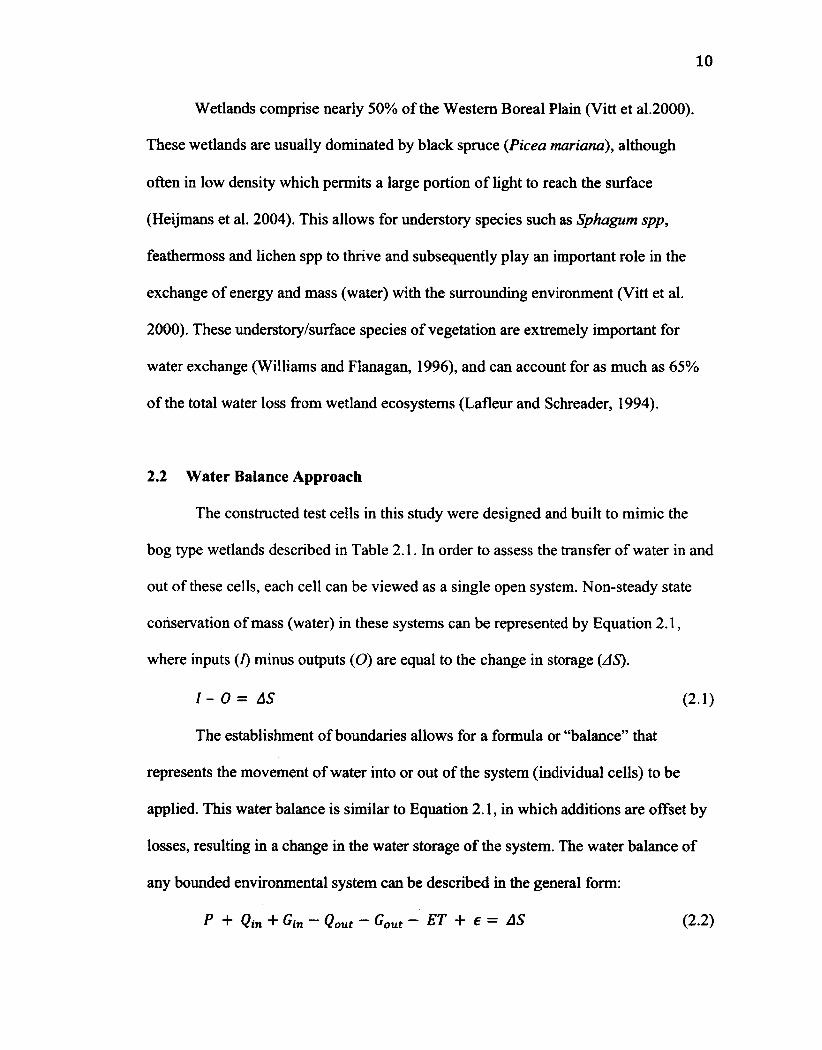
2.2 Water Balance Approach
The constructed test cells in this study were designed and built to mimic the
bog type wetlands described in Table 2.1. In order to assess the transfer of water in and
out of these cells, each cell can be viewed as a single open system. Non-steady state
conservation of mass (water) in these systems can be represented by Equation 2.1,
where inputs (7) minus outputs (O) are equal to the change in storage (/IS).
I - 0= AS (2.1)
The establishment of boundaries allows for a formula or "balance" that
represents the movement of water into or out of the system (individual cells) to be
applied. This water balance is similar to Equation 2.1, in which additions are offset by
losses, resulting in a change in the water storage of the system. The water balance of
any bounded environmental system can be described in the general form:
P Qin + Gin ~ Qout ~ Gout ~ ET + € = AS (2.2)

where, P is precipitation in the form of rain or snow, Q is the surface runoff into or out
of the system, G is the groundwater seepage in or out of the system, ET is
evapotranspiration and AS denotes the change in water storage of the system itself. In
this general form, the components on the left side represent inputs (additions) and
outputs (losses) of the system while the right hand side represents the cumulative
change in storage. Also, an error term, e, is added in order to account for some degree
of measurement error. All terms are typically expressed as a depth of water (e.g. mm).
This general form of the water balance does not apply directly to the study cells
given their design and construction. Therefore, by modifying the general form in
Equation 2.2, a water balance related specifically to the movement of water in each
cell was created (Equation 2.3). The resultant equation quantifies the change in water
storage over time as a function of water related inputs and outputs occurring in each
cell over the study period. There are some important differences between this cell
specific water balance and the general form.
P + Irr - ET - L + e = AS (2.3)
Here, the inputs are composed of precipitation, P, in the form of rain only, and the
water that is artificially added to each cell through the irrigation network, Irr. This
change is important, as the inputs now comprise a much larger component than in a
natural system during the summer growing season where typically intermittent
convective storms provide the vast majority of water inputs to the system. The major
output is evapotranspiration, ET, occurring within each cell. In natural bogs where
lateral movement of water is insignificant, ET is an important component of the water
balance, as it represents the only major loss of water from the system (Baldocchi et al.

12
1997; Wever et al. 2002). Thus, ET should also be a substantial part of the water
balance of each cell as they were designed to function like natural bogs with negligible
transfer of water in or out. A leakage term, L, has been added to represent the potential
for water seepage through the sides or bottom of the cells. The impermeable liner was
designed to keep leakage to a minimum, but they are susceptible to cracks and
punctures. Again, an error term, e, is added in order to account for some degree of
measurement error. Finally, AS denotes the change in water storage of the peat/soil
mixture over the course of the study period and could be positive or negative, although
natural wetlands typically experience a loss in storage during the growing season
(Price, 2003).
2.3 Evapotranspiration
Evapotranspiration (ET) is the movement of free surface water, soil pore water,
and water transpired from vegetation to the atmosphere, and is the process that links
the water and energy cycles (Oke, 1987). ET requires energy; consequently the amount
of energy available at the wetland surface has direct control on ET and other processes.
Net incoming energy (R„) is the net gain in short wave and long wave radiation
(energy) at the Earth's surface. R„ is then dispersed into the environment through
turbulent and conductive forms of transfer, as shown in the surface energy balance
(Equation 2.4).
Rn = LE + H + G + S (2.4)
This equation relates Rn to four processes of energy (heat) distribution: heating of the
soil (G), potential storage within the vegetation and the air column below the canopy

(5), direct transfer of heat energy from surface to atmosphere (H), and energy used for
the latent heat (water vapour) transfer (LE). All fluxes are typically represented in W
m"2 or MJ, and LE is the energy that is consumed in evaporating water from the surface
to the atmosphere and is directly connected to the water balance of any system. Since
ET is the primary loss of water in the study cells, LE becomes a very important process
as it represents the link between their respective energy and water balances.
Latent heat flux, or the amount of energy used for evaporative processes, can
be estimated as a function of the meteorological factors that drive the evaporation
process and surface factors that act to inhibit or enhance it. Although there are
different equations utilized to estimate LE, and subsequently ET, the most widely used
is the Penman-Monteith equation (Equation 2.5) (Monteith, 1981, 1965). The strength
of this equation is that it incorporates a mass transfer (water) component with an
energy balance component in a way that does not require surface temperature
measurements like many other approaches to estimate ET (Dingman, 2002).
Furthermore, it considers both the energy (heat) that drives the ET process (the
diabatic term on the left side of the numerator) with the turbulent transfer of water
away from the surface (the adiabatic term on the right of the numerator). In combining
these approaches, the Penman-Monteith equation is often termed a combination model
and is commonly expressed as:
—G—S~)+pwCwVPDra
4+y(l+rars)
where A (g m"3 °C"') is the relation between saturation vapour pressure and
temperature, (Rn — G - S) (W m"2) is a term representing the available energy, pw (g
m"3) and Cw (J Kg"1 K"1) are the density and specific heat capacity of water

14
respectively, VPD (kPa) is the atmospheric vapour pressure deficit, ra (m s"1) and rs (m
s"1) are the aerodynamic and stomatal resistances respectively, and y (g m"3 °C"') is the
psychrometric constant (Oke, 1987). The derivation of this equation assumes that there
is no advected energy, which is generally not valid for free water bodies but are
usually reasonable when considering a predominantly vegetated surface (Dingman,
2002).
The Penman-Monteith equation may provide information into which
environmental factors influence the rate at which ET occurs. The equation (Equation
2.5) attempts to quantify ET by using five main environmental components that affect
it in some capacity. They are: available energy (Rn — G — S), vapour pressure deficit
(VPD), the saturation vapour pressure curve which is a function of temperature (A),
turbulent mixing of air (ra), and the resistance of the canopy, (rs), controlled by
vegetation through stomata (Lafleur, 2008, Lott and Hunt, 2001). These five variables
are connected to more tangible and measurable micrometeorological factors through
known relations and empirical estimates (Dingman, 2002). Therefore, quantifying and
understanding these five micrometeorological components directly in the field may
achieve a better estimate of ET and an understanding of its controls.
Available energy is the driving force behind ET. Evaporating water requires
relatively large amounts of energy, and this energy ultimately comes from the sun. As
discussed above, the surface energy balance (Equation 2.4) shows how energy is
partitioned among different fluxes, one of which is the latent heat transfer or ET. In
general, during long, mainly sunny days that are common in northern Alberta during
the peak growing season, a large amount of energy is partitioned into the latent heat

15
flux, and subsequently ET is able to proceed at high rates (Humphreys et al. 2006).
Vapour pressure deficit (VPD) is a measure of the ability of the air to receive
water vapour based on an existing gradient. This gradient is the saturation vapour
pressure (e*) for that given temperature minus the actual vapour pressure (e).
VPD = e* - e (2.6)
VPD and air temperature are closely linked since saturated and actual vapour pressures
are highly dependent on temperature (Oke, 1987). Air temperature regulates the
maximum saturated vapour pressure; higher air temperatures can achieve greater
VPD's, thus enhancing the potential for ET.
VPD can act as a control on ET as it expresses an effective demand on surface
moisture, be it open water, soil or vegetation, into the atmosphere. During the day,
vapour pressure is typically greatest near the surface and decreases with height in the
atmosphere; consequently the flux of water vapour is upward, away from the surface
(Lafleur, 2008). The amount of water vapour that is evaporated into the atmosphere is
dependent on the magnitude of the vapour pressure gradient and the degree to which
the atmosphere is able to maintain this gradient by removing moisture from the lower
atmosphere. This is a function of the turbulence in the boundary layer.
Turbulence refers to air mixing occurring in the atmosphere. Mixing generally
occurs as a result of vertical, circular swirling air currents or eddies. Wind velocities
and thermal layering in the atmosphere control near surface eddies (Oke, 1987). In
general, higher wind speeds produce more mixing and greater turnover of air, and thus
a greater potential for water vapour to be moved away from the surface. Ground
features also play a role in affecting turbulence, as obstacles tend to create disturbance,

16
which in turn leads to increased wind speeds and larger eddies (Oke, 1987).
Turbulence is often represented by the aerodynamic resistance term ra, which is a ratio
of the horizontal wind speed (u) to the square of friction velocity of the surface
(u*), both measured in m s"1 (Equation 2.7).
ra = u / (u*)2 (2.7)
Friction velocity is a function of the mean wind speed at a given height and the
surface roughness length. Roughness length is a measure of the aerodynamic
roughness of a surface and is related to the height of the roughness elements. Other
factors such as shape, density and distribution of the elements also affect this variable.
Surface roughness length is commonly estimated as 10% of the height of the surface
elements, which in this study were various types of vegetation (Oke, 1987).
The type of vegetation, near surface moisture status, and the depth to the water
table in the soil can influence how much water is transferred to the surrounding
environment. The ability of vegetation to restrict the release of water into the air is
referred to as surface (or sometimes stomatal) resistance (rs). Vegetative controls on
ET, via surface resistance, are an integral part of the seasonal energy and water balance
of Boreal bogs and fens (Brown et al. 2010). Surface resistance is dependent on many
vegetative and environmental factors and often varies greatly through time and space.
Perhaps the most important environmental factor that affects surface resistance is the
availability of water. Vegetation tends to close its stomata during prolonged periods of
stress, which can be caused by, among other genetic and environmental factors, little
or no access to water (Dingman, 2002). The depth of the water table below the surface
can have a control on the availability of water for ET through free surface or soil

evaporation or via plant uptake and subsequent transpiration. Although water
availability is not explicitly considered in the Penman-Monteith equation (Equation
2.5), it can still be an important factor affecting ET (Ingram, 1983; Lafleur et al. 2005).
This may be especially true in northern regions (such as the study site) that often have
relatively dry growing seasons (Humphreys et al. 2006).
Overall, the Penman-Monteith equation is widely applied because it provides a
framework that incorporates both biotic and abiotic elements that control ET in a
vegetated zone (Baldocchi et al. 2000). However, the application of evaporation
models based on homogenous land cover, like the Penman-Monteith equation, to
wetlands creates potential problems relating to the spatial scale of measurements
(Lafleur and Rouse, 1988). Wetlands are generally composed of heterogeneous land
cover, with patches of wet and dry areas, which may have very different values for
many of the factors used in the Penman-Monteith equation and thus may lead to point
estimates of ET being unrepresentative of the wetland as a whole (Gavin and Agnew,
2003).
2.4 Previous Research
Wetland ET research began when urban expansion prompted the need to
determine the best way to drain and/or clear wetlands (Drexler et al. 2004). More
recently, interest in wetland ET has come from the need to understand the processes
and function of these ecosystems, particularly from a management perspective. There
has been considerable effort studying natural, disturbed and constructed wetlands to
quantify the water balance (of which ET is a major component) in an attempt to

determine their water requirements and hydrological regimes (Carter, 1986;
Rosenberry and Winter, 1997). This information can be used to measure fluxes of
contaminants or nutrients, transpiration habits of wetland vegetation,
phytoremediation, groundwater modeling and even global climate modeling (Drexler
et al. 2004). Still, wetland ET remains poorly characterized due to the high variability
in both space and time (Souch et al. 1996). Drexler (2004) suggests that this may be
caused by the relative differences in the multitude of techniques used to measure ET
and/or the fact that it is challenging to obtain reliable results given the lack of
uniformity in shape, surface cover, hydrology and topography of wetlands. In this
section some of the past research in wetland ET that is relevant to this particular study
will be presented.
2.4.1 Vegetation and E T
Along with free water and soil water sources, the contribution to ET from
vegetation is considered an integral component of wetland ET, where processes at the
vegetation community scale affect the total ecosystem exchanges of water (Brown et
al. 2010). The exact vegetation composition within Boreal wetlands is dependent on
the spatial variability of the surface moisture characteristics. The interaction between
vegetation and moisture conditions may be even more important to Boreal bogs and
fens because of limited lateral flow gradients (Devito et al. 2005). This lack of water
movement has been shown to enhance components of vertical moisture exchange,
perhaps amplifying the importance of surface moisture-vegetation interactions
(Smerdon et al. 2005). Williams and Flanagan (1996) suggest that concentrated
moisture patterns only act to encourage vertical water movement and are often

prompted by gradients between moisture rich peat and the drier air above.
During dry periods, vegetation and soil are more resistant to water movement
into the atmosphere (Lafleur, 2008). Since different plant species have differing
abilities to conserve or release water, plant type is a very important consideration for
ET. Water loss from mosses and other non-vascular plants differs from that of vascular
plants. During photosynthesis in vascular plants, water coming mainly from their roots
is released as vapour through stomata on their leaves and stems. Because vascular
plants have extensive systems of roots allowing fairly consistent access to water, ET in
wetlands rich in vascular plants often relies on the transpiration capacity of the plant
canopy itself (Heijmans et al. 2004). In contrast, mosses evaporate water from their
surface rather transpiring like vascular plants. Tightly packed single leaves and water
holding structures (known as hyaline cells) that are supported by the small branches of
the capitulum. These tightly packed cells force water through the capitulum where
water is evaporated (Lafleur, 2008; Ingram, 1983). Mosses do not have a water
transport system like vascular plants, and their stems do not conduct any water. The
dead leaves and branches create a network of small pores and water moves up through
this network and from the sides of the stems due to capillary gradients. If the water
table is at or near the surface, the network will work efficiently because water can
diffuse across small distances. However, if the water table is lower, the stems will not
be in contact with water, and the transpiration rates will decrease (Lafleur et al. 2005).
As mosses dry out they are unable to draw water to the surface efficiently, and so
significant decreases in ET are possible. Several studies have noted a sharp decline in
ET rates as mosses dry out and are unable to move water through capillary action

(Price, 1991; Kim and Verma, 1996).
To better understand the movement of water within northern bogs and fens,
Price et al. (2009) performed a laboratory experiment to study the mechanisms of
water transport within Sphagnum moss and from the moss into the atmosphere. The
authors transplanted small pieces of moss and, using controlled environmental
conditions (air temperature, relative humidity, amount and duration of incoming solar
radiation, and air mixing), measured the subsequent ET. Their results confirmed that
water flux in Sphagnum while undergoing ET is predominantly in the form of liquid
capillary diffusion. The results also confirmed, surprisingly, that despite large pore
spaces present in peat, water vapour movement below the surface was a negligible
portion of net water flow. ET ranged from 3.9 mm d"1 to 4.8 mm d"1, with an average
of 4.5 mm d'1 under constant environmental conditions (average T=20.7 °C,
RH=31.3%, 12 hours of artificial UV light per day, constant air circulation). The
authors also found that a portion of the latent heat flux occurred below ground,
creating the potential for errors when trying to estimate the available energy to perform
ET. They suggest that models such as the Penman-Monteith equation (Equation 2.5)
may have limited validity in moss dominated systems given that such models assume
that radiative and convective fluxes occur at a common reference surface.
The manner in which water becomes available to plants and mosses has been
studied in both natural and disturbed wetlands. Lafleur et al. (2005) studied ET over 5
growing seasons at a natural bog in eastern Ontario and found that ET was weakly
related to the depth of the water table. ET appeared to be affected by the depth to the
water table only when it dropped below a specific threshold, which was thought to be

associated with the rooting depth of the vascular plants at the site. The concept of a
critical water table threshold was also suggested in previous studies, such as Ingram
(1983), Nicholas and Brown (1980), and Lafleur et al. (2005). Price (1996) studied a
disturbed and an undisturbed section of a bog complex in northern Quebec and found
that changes in the composition of the underlying soil can greatly reduce the specific
yield (water holding ability) of peat and cause exaggerated water table changes in
disturbed wetlands. The study concluded that poor moss growth on disturbed surfaces
can often be attributed to the inability of mosses to obtain water from the underlying
peat, which holds water at greater suction than non-vascular plants like mosses can
generate.
2.4.2 ET in Natural Systems
ET in natural bogs and fens is quite low compared to that in other wetland
systems such as marshes and swamps (Lafleur, 2008). However, ET in bogs and fens
may still approach the maximum potential rate possible for the given environmental
conditions. Near maximum potential ET in bogs and fens may occur under at least one
of the following conditions: (i) a large amount of the surface area is open water (Price,
1994), (ii) the area is dominated by vascular vegetation (Lafleur, 1990), or (iii) the
moss cover is moist because of dew, fog or rain (Price, 1991). Vegetative controls and
hydrologic restrictions can limit ET in bogs and fens. A compilation of many studies
conducted across Canada that have measured actual ET rates of wetlands is shown in
Figure 2.1. Many of these studies observed that Sphagnum dominated bogs and poor
fens had the smallest mean ET rates. Meanwhile, rich fens, which are dominated by
vascular plants, and other wetland types common to lower latitudes such as swamps,

22
were observed to have similar ET rates, higher than those of bogs and poor fens
(Lafleur, 2008). Marshes, which are dominated by aquatic vegetation such as tall
reeds, had the highest ET rates.
Bog Rich fen Poor fen Marsh Swamp
Figure 2.1 Comparison of tabulated daily ET rates from a collection of Canadian studies. Boxes show the mean daily rate while whiskers denote the min and max observed values. The number above and to the right of the boxes indicates the number of studies used in compiling the results. Bog and poor fen types, common to the boreal region have relatively lower ET rates than other wetland types (from Lafleur, 2008).
Roulet et al. (1997) compiled data from studies on wetlands from across
Canada and had similar findings regarding wetland ET. Bogs had the lowest measured
maximum ET rate (0.4 mm hr"1). Meanwhile, maximum ET rates for fens were
observed to be slightly higher than those for bogs (0.52 mm hr"1). Brown et al. (2010)
reported comparable rates from a typical wetland system of the western boreal plains,
dominated by mosses and sparse vascular vegetation. Peak ET ranged from 0.2 - 0.6
mm hr'1 depending on location, vegetation composition and time period. Of note was
that Sphagnum ET rates were greatest early in the growing season (0.6 mm hr"1) but
began to decrease as the season progressed, while lichens were observed to have

23
higher ET rates late in the growing season (0.4 mm hr"1). The authors commented that
different varieties of non-vascular vegetation control ET differently throughout the
growing season, and so should be considered a key component of wetland water
balances at the sub-landscape scale.
Humphreys et al. (2006) reported on ET measurements of several northern
wetland systems ranging from bog to extreme-rich fen. Midday ET ranged only from
0.21 - 0.34 mm hr"1 despite a wide range of vegetation types and combinations in each
wetland. One key finding was that ET was primarily driven by radiation at all sites,
particularly when water availability was not a restriction and when VPD was high. As
sites dried up, ET rates dropped, particularly at sites with many vascular plants and
trees but less so at sites with significant Sphagnum spp cover. Kellner (2001) also
noted vegetative controls decreasing ET rates in conditions thought to yield high ET
rates (e.g. high Rn and VPD). In this study of a Swedish wetland, ET was again most
strongly linked to radiation than to any other controlling factor. Furthermore, there was
a strong trend between rising stomatal resistance (rs) and increasing VPD. In contrast,
vegetative conductance showed a weakly negative correlation with available energy,
decreasing slightly under sunnier conditions (increased radiation). These findings
suggest that although ET is driven by four controlling factors, vegetative responses to
these controlling factors may also be an integral mechanism in the process of ET.
(Kellner, 2001)
2.4.3 ET in Disturbed and Constructed Wetlands
Disturbance of a wetland causes changes to its physical properties, the depth to
the water table and the vegetation, and consequently may have implications for ET at

24
reclaimed sites. Peat that is exposed during disturbance can actually have a higher
water retention capacity (specific retention; Sr) than living or non-decomposed dead
mosses (Schlotzhaur and Price, 1999), due to its finer pore structure and higher bulk
density (Okruszko, 1995). The changes in disturbed peat may allow capillary
movement of moisture to more readily sustain surface moisture compared to
hummocks in natural wetlands (Price and Waddington, 2000). Thus, changes in peat
properties can help supply the evaporating surface with sustained moisture. Based on
this process, and other vegetative and drainage factors, Van Seters (1999) suggested
that total ET (losses) may increase with time elapsed since disturbance and/or
abandonment. The notion of ET increasing after disturbance has been suggested in
other studies. Petrone et al. (2003) found that restoration techniques that resulted in a
higher water table, higher soil moisture and the re-emergence of vascular plants
created higher ET losses than in an adjacent unrestored site. It was suggested that not
only did the increased density of vascular plants increase transpiration but that it also
increased surface roughness, which further enhanced ET through greater turbulent
transfer.
ET at disturbed sites may be more spatially variable, due to changes in soil
properties and vegetative conditions. In a two-year study, Van Seters and Price (2001)
found that average ET rates at a disturbed (harvested) bog were similar to that at a
nearby undisturbed bog, but showed much more variability of ET rates depending on
location. ET rates were lower in raised areas (1.9 mm d"1) and much higher in lower
areas and/or ones of high moisture where Sphagnum was present (3.6 mm d"1),
resulting in an average similar to that at the natural site (2.9 mm d'1). The authors also

found that ET represented the greatest loss of water from the disturbed site over the
two growing seasons being studied. ET was responsible for 92% and 84% of water
loss during 1997 and 1998 respectively, with runoff from slopes and ditches making
up the remaining portion. The water balances of the disturbed site showed that ET was
much larger than precipitation, 1.4 and 1.3 times greater in 1997 and 1998
respectively. This difference resulted in substantial decreases in water storage, -75 mm
and -100 mm in 1997 and 1998 respectively, compared to a -58 mm (1998 only)
decrease in water storage at the natural site. The decreases in water storage was
thought to have been responsible for greater depth to, and fluctuations of, the water
table at the disturbed site, and may be a major factor in limiting regeneration and
reestablishment of natural wetland functioning. It was suggested that these spatial
variations in ET and runoff resulted in a much different water balance than that of a
relatively uniform distribution of losses common in natural bog systems.
It is not yet fully understood how ET occurs in constructed wetlands, as
compared with natural wetlands. Lott and Hunt (2001) studied a constructed wetland
complex built directly adjacent to an existing natural fen in the northern United States.
As measured by a weighing lysimeter, the constructed fen had a significantly lower
daily ET rate (3.5 mm d"1) throughout the growing season than the natural site (5.6 mm
d"1). Given the relative consistency of other environmental and climatic factors, it was
suggested that this difference was attributable to differences in the availability of water
in the rooting zone and the timing of plant senescence.
Campagam and Waddington (2008) studied the effects of upper layer
(acrotelm) peat transplanting on hydrologic properties and function. They compared a

natural portion of wetland to a section that had recently been harvested using the
trench extraction restoration technique. This method involves the removal of the
vegetative acrotelm (1-2 m), harvesting a portion of the thicker, denser lower layer
(catotelm) beneath and then replacing the acrotelm back on top of the now much
deeper and older catotelm. They found that the transplanted site maintained a higher
water table compared to the natural site but that this did not result in higher volumetric
water content (VWC) at the surface as would be expected. The authors suggested that
the removal and replacement of the acrotelm might have damaged it structurally,
resulting in great variation in VWC at the surface. This in turn may alter its ability to
move water up through the profile for exchange with the atmosphere through ET in the
same fashion as undisturbed peat. ET at the transplanted site was estimated to be over
two times (10 mm d"1) that at the natural site (4-5 mm d"1) by using a mass balance
approach and quantifying daily fluxes in VWC. It is hypothesized that this extreme
diurnal change in VWC is partially related to the aforementioned changes in the peat
structure and not just to ET alone, even though soil moisture characteristics were
similar at both sites. The acrotelm was extracted in large blocks, retained and then
placed onto exposed peat leaving large spaces or gaps between them, which can cause
significant changes in the peat structure. The authors suggested that the lateral
movement (expansion/contraction) within the peat matrix might be exaggerating the
apparent fluctuations of VWC, and consequently of ET.
Drexler et al. (2004) outlined two important phenomena that may affect ET at
the study site, namely its shape/size and its geographic location. First, wetlands
surrounded by areas with low ET such as bare soil, tend to have higher ET than

27
wetlands surrounded by forest. This is known as the "oasis effect". Second, long
narrow wetlands and those on the fringes of lakes and rivers tend to have higher ET
than large expanses of wetland that have higher ratios of area to perimeter - known as
the "clothesline effect". The oasis effect is a result of advection over areas of differing
moisture creating sharp gradients in VPD and other factors while the clothesline effect
occurs because of increased ventilation through a smaller, more isolated canopy
(Linacre, 1976). The site in which the current study was performed may be subject to
both the oasis and the clothesline effects. It is completely surrounded by mining
operations composed of predominantly dry and bare soils. The cells (test plots) are
very small for wetlands and so have a very small area to perimeter ratio. The processes
discussed above are normally not of great concern when studying natural wetlands but
could be extremely important in the construction of wetlands adjacent to major mining
and development operations as is the case here.

28
3.0 Study Site and Methodology
3.1 Study Site
The study site is located approximately 40 km NNW of Fort McMurray,
Alberta (57° 03.8' N, 111° 39.8' W, elev.~370 m) (Figure 3.1). The region has a
continental Boreal climate, with mean monthly temperature ranges from -18.8°C to
16.8°C (Jan. - Jul.) and an average annual precipitation of 456 mm, of which
approximately 220 mm typically falls during the study period (DOY 152 to DOY 230
-June 1st to August 18th, 2010) (Environment Canada, 2011). The growing season for
the Fort McMurray region is relatively short, with an average of 157 frost-free days
(Environment Canada, 2011).
Syncrude Ltd Mildred Lake Mine
Study Site
CANADA
Fort McMurray
Fort McMurray
iKm
Edmonton
Calgary Vancouver
Regina
S <0100 200 300 400 IKm
Figure 3.1 Location of Fort McMurray in northern Alberta, Canada and the study site situated 40 km northwest of the city within Syncrude Canada Ltd. Mildred Lake Mine (inset).

29
The study site is located in the northern section of Syncrude's Mildred Lake
Mine on an elevated hilltop that is just west of the current active mine (Figure 3.2).
The site is surrounded by land disturbed by construction and mining activities. North
of the site is a large expanse of dry processed sand while to the east is an open storage
area where industrial equipment is stored. To the west of the site is a shallow reservoir
of fresh water and to the south there are a series of dirt roads with intermittent
vegetation cover. The study site and its adjacent land cover can be seen in Figure 3.3.
U-Wnped Coa krigrton Layout MLS8. Juna 2010
Figure 3.2 As built plan showing location of the study site within the mine (inset) site setup including irrigation networks and surrounding land cover (from BGC, 2010).

(b)
m n
Figure 3.3 Aerial view of study (a) and oblique view of an individual cell (b).

The site, called the U-Shaped cell, was previously a composite tailings site in
the southwest portion of the Mildred Lake Settling Basin. From August to November
2008 the site was covered with clean clay reclamation material and then transformed
into series of small, disconnected rectangular pits about one metre deep. Each
rectangular pit, or "cell", measured approximately 20 m by 13 m. The pits were
separated by narrow ridges of clay that created small pathways between the cells. Each
cell was then lined with an impermeable synthetic liner (20 mm Enviroflex
Geomembrane) and then overlain with 20 cm of compacted clay. The construction
process is detailed in Figure 3.4. Great attention was placed on the design and
installation of the cell liners in order to prevent water from entering or leaving, either
laterally or vertically, through the sides or base of the cells. The effectiveness of the
liner to isolate cells from the surrounding environment is uncertain, and will be
discussed more in the Results and Discussion sections.
The test cells received different treatments that represent potential wetland
construction and regeneration techniques. Syncrude has defined and implemented
several combinations of construction techniques that are thought to be suitable and
feasible, specifically for this environment. The present study monitored six treatment
combinations that were applied in both summer and winter 2008, involving a total of
12 cells. Treatment variables included: i) the origin of the vegetation, ii) the depth of
the soil/peat mixture and iii) the season in which the treatment combinations were
applied (Table 3.1). Vegetation in the cells was from either a live transplant from a
nearby natural fen slated for mining or from seedlings grown in a greenhouse and
planted in the spring of the first year. The transplanted vegetation was removed

32
(C) <D)
Figure 3.4 Lining of the cells involved digging a trench at the edge of the cell (A) manually stretching geosynthetic liner over base of cell (B) covering with 20 cm of clay (C) and compacting (D) (from BGC, 2009).
using specialized equipment from a nearby fen that was slated for mining. A large
scoop with a flat bottom was used to obtain large square blocks of peat including
surface vegetation, which were then secured and transported to the site. The blocks had
thicknesses of roughly 15, 50 or 100 cm. The cells that did not receive a live transplant
were filled with a stockpiled mixture of organic debris and peat. This stockpiled
mixture is collected as nearby areas are cleared for mining and the top organic layer is
processed and stored in piles on site for future use as a soil cover. The stockpiled

33
mixture was also laid down in depths of 15, 50 or 100 cm after which greenhouse
vegetation was planted by hand. Each treatment combination was applied either in
summer (September 2008) or winter (January 2009) to assess the affect of seasonality
on soil/peat harvest and placement, and vegetation started in greenhouses were planted
the following spring.
Table 3.1 Treatment combinations for each of the 12 study cells.
Cell Soil/Vegetation Origin Peat/Soil Mixture Application Season Name Depth
S-P-100 cm Live transplant from nearby natural wetland
100 cm Summer
S-P-50 cm Live transplant from nearby natural wetland
50 cm Summer
S-P-15 cm Live transplant from nearby natural wetland
15 cm Summer
W-P-100 cm Live transplant from nearby natural wetland
100 cm Winter
W-P-50 cm Live transplant from nearby natural wetland
50 cm Winter
W-P-15 cm Live transplant from nearby natural wetland
15 cm Winter
S-S-100 cm Planted seedlings in Stockpiled mixture
100 cm Summer
S-S-50 cm Planted seedlings in Stockpiled mixture
50 cm Summer
S-S-15 cm Planted seedlings in Stockpiled mixture
15 cm Summer
W-S-100 cm Planted seedlings in Stockpiled mixture
100 cm Winter
W-S-50 cm Planted seedlings in Stockpiled mixture
50 cm Winter
W-S-15 cm Planted seedlings in Stockpiled mixture
15 cm Winter

34
In an attempt to replicate natural wetland conditions, the water table was
artificially kept at, or very near, the surface by adding fresh water to each cell from a
reservoir through a pipe system. The system consists of two irrigation loops, with each
loop having an intake at the reservoir and release valves at each of the cells that it
serves. During the late summer when the reservoir was low, water was brought in by
truck and directly connected to the irrigation system.
Vegetation in the cells differed considerably between the transplanted cells and
those made of a stockpiled peat mixture. The transplanted cells have a mixture of
typical boreal fen vegetation and emergent vegetation that have established since
construction. Native species include: Labrador tea (.Ledum groenlandicum), bog
blueberry (Vaccinium uliginosum), bog cranberry ( Vaccinium oxycoccos), cotton grass
(Eriophorum virginicum), horsetail (Equisetum spp), black spruce (Picea mariana),
dwarf birch (.Betula pumila), and Sphagnum spp. Emergent vegetation in the
transplanted cells include large groups of cattails (Typha latifolia), foxtail barley
(Hordeum jubilatum), field horsetail (Equisetum arvense), fireweed (Epilobium
augustifolium), celery leaved buttercup {Ranunculus sceleratus), water sedge (Carex
aquatilis), ribbon grass (Phalaris arundinacus) and grasses Salix spp and Poa spp.
The stockpiled cells contain a less diverse mix of vegetation as only a few
species that were thought to have a high chance of success were planted. These species
include water sedge Carex aquatilis, ribbon grass Phalaris arundinacus, tickle grass
(Agrostis scabra), along with small trees such as dwarf birch (Betula pumila) and
tamarack (Larix larcina). Similar to the transplanted cells, emergent species such as
cattails (Typha latifolia), barley foxtail (Hordeum jubilatum), and western dock

35
(Rumex longifolius), as well as grasses Salix spp. and Poa spp. have established over
large areas of the stockpiled cells and in some cases are now the dominant species.
Other minor emergent species in the stockpiled mixture cells include: perennial sow
thistle (Sonchus arvensis), ball mustard (Nesia paniculata), narrow leaved hawksbeard
{Crepis tectorum), small bedstraw (Galium trifidum), celery leaved buttercup
(Ranunculus sceleratus), and cinquefoil (Potentilla norvegica). A more detailed
summary of the vegetation found in each type of cell is listed in Table 3.2 with photo
examples shown in Figure 3.5.
36
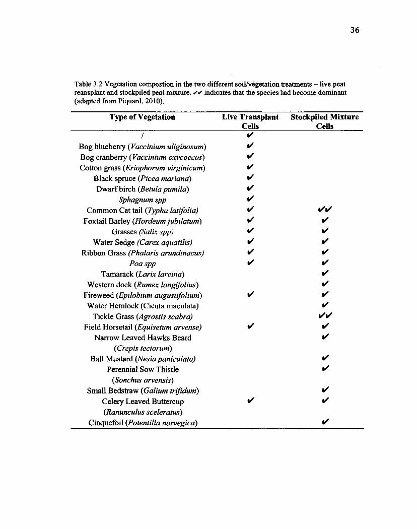
Table 3.2 Vegetation compostion in the two different soil/vegetation treatments - live peat reansplant and stockpiled peat mixture. // indicates that the species had become dominant (adapted from Piquard, 2010).
Type of Vegetation Live Transplant Stockpiled Mixture Cells Cells
/ •
Bog blueberry (Vaccinium uliginosum) •
Bog cranberry (Vaccinium oxycoccos) •
Cotton grass (Eriophorum virginicum) •
Black spruce (Picea mariana) •
Dwarf birch (Betula pumila) •
Sphagnum spp •
Common Cat tail (Typha latifolia) • ••
Foxtail Barley (Hordeum jubilatum) • •
Grasses (Salix spp) • •
Water Sedge (Carex aquatilis) • •
Ribbon Grass (Phalaris arundinacus) • •
Poa spp • •
Tamarack (Larix larcina) •
Western dock (Rumex longifolius) •
Fireweed (Epilobium augustifolium) • •
Water Hemlock (Cicuta maculata) •
Tickle Grass (Agrostis scabra) ••
Field Horsetail (Equisetum arvense) • •
Narrow Leaved Hawks Beard •
iCrepis tectorum) Ball Mustard (Nesia paniculata) •
Perennial Sow Thistle •
(,Sonchus arvensis) Small Bedstraw (Galium trifidum) •
Celery Leaved Buttercup • •
(Ranunculus sceleratus) Cinquefoil (Potentilla norvegica) •

37
Figure 3.5 Vegetation found in stockpiled cells (a) and live peat transplant cells (b) on July 7th 2010 (DOY 188).

38
3.2 Field Methods
The study ran for most of the 2010 growing season. Meteorological
measurements began on DOY 152 (1st June, 2010) and ended on DOY 230 (18th
August, 2010).
Instruments were installed at a height of 2.8 m at a central location at the site.
Air temperature and relative humidity were measured using a hydrometer (HMP35,
Vaisala). Wind speed was measured with a cup anemometer (Met One 014A,
Campbell Scientific). All instruments were connected directly to a data logger (CR23x,
Campbell Scientific); measurements were taken every five seconds and averaged over
30 min intervals.
Incoming short-wave radiation was measured with a pyranometer (SP Lite,
Kipp and Zonen) located at a meteorological tower approximately 1 km away, which
was sufficiently close to have had similar sky conditions over the course of a day.
Incoming solar radiation (Kj) comprises the largest component of the available energy
and thus can provide a reasonable indication of available energy on a daily basis (Oke,
1987). Because of logistical constraints, and given the strong relationship between
solar radiation and net radiation (R„), incoming solar radiation (K|) was measured in
place of net available energy.
Precipitation was measured using a tipping bucket rain gauge (TE 525M, Texas
Electronics). Daily precipitation totals were also cross-referenced against
measurements made at the Fort McMurray airport by Environment Canada. Although
there is some agreement between the two sets of measurements, there are also
considerable differences in both the magnitude and timing of precipitation as summer

39
rainfall is largely convective in nature and is dominated by high intensity short
duration storms with high spatial variability.
ET was measured using manual weighing lysimeters (Figure 3.6). One clear,
rectangular, plastic box of 6.5 L volume was installed in a representative location in
each cell. Vegetation and soil were carefully removed with a cutting device and placed
in the lysimeters, which were then re-installed flush with the surrounding terrain. Each
lysimeter was weighed daily (logistics and weather permitting) on a 20 kg capacity
scale with 0.5 g precision (EB15, Ohaus), and change in mass was recorded. Moisture
in the lysimeters was maintained at levels similar to the surrounding terrain by
checking with a TDR moisture probe every few days and adding or removing water,
and recording the new mass.
The near-surface temperature of each cell was measured using a soil thermistor
(109B, Campbell Scientific). Wind speed approximately 2.8 m above the evaporating
surface was measured with a cup anemometer (014A, Met One), averaged over 30
minute periods, and sent to a data logger (CRIOx, Campbell Scientific).
The water table depth of each cell was recorded using a logging pressure
transducer (Levellogger JR model 3001 and Barrologger, Solinst) located in a
standpipe piezometer. The pressure transducer made readings every 10 minutes, and
the readings were corrected for atmospheric pressure variations. Daily manual
measurements of well stick-up height, depth to water in the well and peat reference
height were also made.
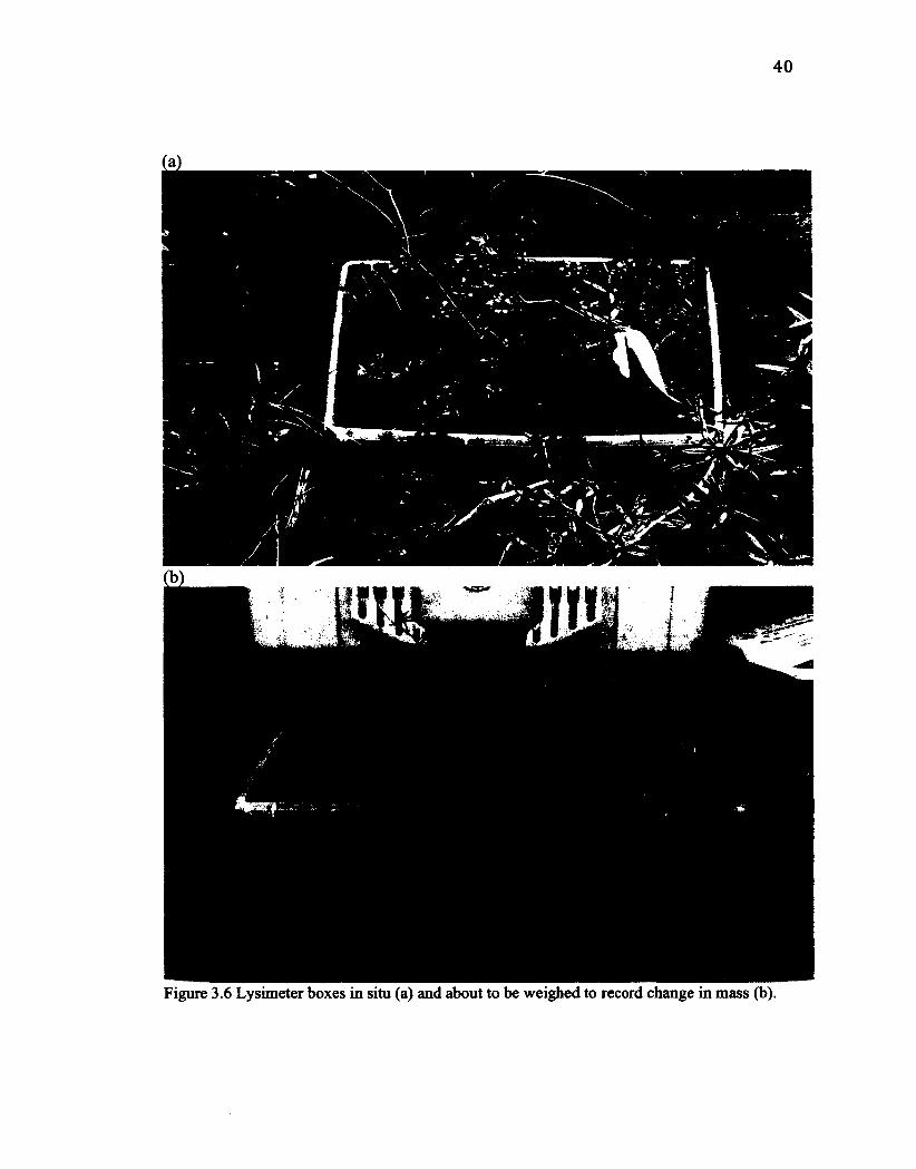
40
Figure 3.6 Lysimeter boxes in situ (a) and about to be weighed to record change in mass (b).

41
The Leaf Area Index (LAI) was assessed at five locations directly adjacent to the
boardwalks in each cell, every 2-3 weeks from DOY 175 (23 June, 2010) to DOY 228
(16 August, 2010), using a LAI-2000 plant canopy analyzer (LI-COR) with a 180°
view restriction. This restriction was used to remove any potential interference created
by the boardwalks. Measurements were made under both cloudy and clear sky
conditions, typically during early or mid afternoon. In situations where the LAI-2000
could view foliage lit by direct sunlight, the possibility of LAI being underestimated
increased. An attempt was made to reduce direct beam radiation by casting a shadow
on the sensor (if it was not a completely cloudy day), as suggested in the LAI-2000
instruction manual.
3.3 Analytical Methods
3.3.1 Irrigation
Because multiple cells were watered at the same time, irrigation volumes had
to be calculated using the Hardy Cross method (Cross, 1936). This technique uses an
iterative method to determine the flow inside a circuit of multiple branches in which
given static conditions are known, but the flow within each branch and out of open
valves is not (Lopes, 2003). The output volume will vary depending on which valves
are open, and the length of pipe between valves. The conservation of mass and energy
dictates that flow arriving at a node must equal the sum of the flows leaving the node.
Qi + <?2+--0n ~ Qn-i = 0 (3.1)
Pressure, or head loss between valves, which affects flow rate, can be described by the
generalized Bernoulli equation:

42
(3.2)
Here p is pressure, p is the fluid density, v is the velocity of the fluid, g is the
acceleration due to gravity and z is the height of each valve. Head loss is directly
related to flow rate under constant conditions and so the flow rate at each valve can be
estimated and corrected iteratively based on the relation of head loss to flow rate:
where Q is the volumetric flow rate, g is the acceleration due to gravity, d is the pipe
diameter, L is the branch length and/is the Darcy-Weisbach friction factor.
Daily irrigation volumes were found using the Hardy Cross method software
application produced by Thermal Analysis Systems (1998). This software requires that
open valves, the lengths and direction of flow between them, given conditions such as
pipe diameter and pressure, along with an estimated flow rate at each valve. A simple
example circuit is shown in Figure 3.7. A network diagram was created for each
combination of open valves that was used in the irrigation process of the study cells.
Input parameters included the number of open valves and the equivalent length of pipe
between each valve, the diameter of the pipe (2 inch) and its friction factor, the
temperature, viscosity and density of the fluid (water), and the assumed initial pressure
and flow rate of the loop.
(3.3)

43
Valve 3 Valve 4 Valve 5 Valve 6 Valve 7 Valve 8 Valve 9 Valve 10 Valve 11
17.3m 16.7m 17.4m 17.1m 16.8m 18.0m 16.1m 15.2m
18.1m
26.8m 1.8m 28.0m
4 *1 T Flow path U ,f
27.7m 27.8m
Valve 2 Valve 1
1 1 20.1m
Valve 14 Valve 13 Valve 12 31.4m
Inlet
Figure 3.7 The irrigation network setup used for finding iterative solutions to pipe and valve flow rates using the Hardy Cross method. Valve outflow varied according to the number and position of open valves and the distance between them.
Each circuit was given an arbitrary flow direction and assumed flow rates at
each valve for a variety of situations in which multiple valves around the circuit were
opened. The software iteratively found the actual flow rates in each section of pipe
between each valve under the given conditions. The flow rate out of each valve is then
the difference between the flow rates of the pipe sections on either side of the valve.
This flow rate was then multiplied by the number of minutes each combination was in
operation on any given day. Irrigation volumes were then converted to a depth in mm
by converting litres to m3 and then dividing by the surface area of each cell. However,
it is very difficult to verify the accuracy of applying this method to this situation.
Because irrigation volumes had to be back calculated, this method can provide only
estimates of irrigation volumes. These calculations require several assumptions and
thus increase the potential for error.

44
3.3.2 Data Processing
Daily lysimeter mass changes were converted into a depth of water equivalent,
using the volume and surface area of the container. Mass changes were not recorded
on days in which heavy rain occurred but were recorded on days in which small
accumulations, generally < 0.5mm, were recorded by the tipping bucket rain gauge on
site. These depths were added to the ET depths according to the time in which they
occurred thus correcting for small additions of water into the lysimeters during days
with minor rain events. Days with heavier rain events often resulted in mass increases
in the lysimeters and so were given an ET value of zero. Daily cell ET was summed
over the study period in order to estimate losses of water from the system.
Environmental variables were averaged and logged in half-hour increments
throughout the entire study period. In order for environmental variables to match the
timing of ET measurements, daily averages were computed from noon to noon as
opposed to actual date change (midnight to midnight).
Water level data was scanned for anomalous data points caused by the
disturbance of the logger during other measurements in the well or water sampling.
These disturbances generally only lasted for a few minutes but often affected the
pressure transducer for hours while the pressure in the logger stabilized. A small
number of anomalous data points were removed. After this, a water table offset was
created in order to calculate the actual position of the water table above or below the
ground surface, as opposed to just a measure of the amount of water above the
transducer.

3.3.3 Soil Properties
In order to determine soil properties, cores were taken from each cell using a
peat profile sampler (Wardenaar, Eijkelkamp). The sampler was pushed vertically
down into the peat in a back and forth motion to the point where the base of the corer
hit denser material, (clay), which marked the base of the cell. Once the core was
removed and brought to the surface a small portion of clay liner that was picked up in
the sampler was removed. Cores measured 10 cm by 12 cm and varied in depth
according to each particular cell. Each core was then wrapped tightly in plastic wrap
and placed into pre-made wooden cases designed minimize disturbance to the cores.
Figure 3.8 shows the steps of the sampling process. Samples were shipped back to
Carleton University. Cores were frozen and then, using a band saw, cut into 5 cm
sections of known volume in order to asses soil properties.
Specific yield is the volume of stored water released per unit surface area, per
unit decline of water table (Dingman, 2002). Specific yield of each section was
calculated by obtaining their 24-hour drainage curves. Sections were thawed for 24
hours, placed in containers, and completely saturated (24 hour soak). Samples were
then allowed to drain through a filter (#1, Whatman), with their change in mass being
recorded every few minutes at first, then every hour with a final measurement after 24
bom's. Conversely, the relative volume of water retained in the aquifer during a water
table drop is referred to as specific retention (Dingman, 2002). Specific retention can
be estimated as the difference between one and the specific yield.

46
The sections were then placed in an 80°C oven for 24 hours to evaporate all
remaining water. Once dry, bulk density of the sections was calculated. Bulk density
was calculated according to equation 3.4:
mdry
~ vs
.-3\ • u.,11, A u. /„ -3\
Pt = -f2 (3-4) VS
where pb (g cm ) is the bulk density of the sample (g cm ), mdry is the mass of the
oven-dried sample, and is the volume of the section. From the estimation of bulk
density, porosity of the samples can be estimated using equation 3.5
0 = 1-^ (3.5) Ps
0 represents porosity (no units), pb is the bulk density of the subsection and ps is the
organic particle density. Organic particle density has been noted to range from 1.0 to
1.5 g cm"3 depending on the degree of decomposition (Young and Spycher, 1979;
Golchin et al. 1994; Hassink, 1995; Ladd et al. 1995; Skopp, 2000; Ellies et al. 2003).
Decomposition was moderate so a value of 1.3 g cm'3 was selected for the organic
particle density.

47
Figure 3.8 Soil Sampling using the Wardenaar peat profile sampler.

48
3.3.4 Statistical Analysis and Modeling
Data was prepared in Microsoft Excel (2011) and then imported into R
statistical software (R Development Core Team, 2009) for further analysis. ET by cell
and micrometeorological factors were organized as a daily time series. Certain
environmental variables related to ET were calculated from existing measurements.
For example, as VPD was not measured directly, it was determined using the air
temperature and relative humidity (RH). Also, depth of the water table from the
surface had to be determined using the levellogger data and the manual well stick-up
height.
Descriptive statistics, histograms and quantile-quantile plots were used to
assess data normality in order to determine appropriate statistical tests. The majority of
the variables were reasonably normally distributed. However, some groups of data,
specifically cell ET time series that lacked a sufficient number of measurements,
showed some skeweness and/or kurtosis. Where necessary, non-parametric tests were
conducted.
The ET data sets for each cell were grouped according to treatment variable to
test the effects of different treatment methods on evaporative losses over the study
period. As some ET groupings were significantly skewed, a Wilcoxon rank-sum test
was used to test differences among the treatments variables of placement period and
soil/vegetation type (2 levels). Differences attributable to soil depth (3 levels), were
tested using one-way ANOVA based rank-sum tests. Each test was performed at the
95% significance level. These tests provided information into which treatment
variables may have had an effect on ET.

49
In order to gain insight into which environmental factors may have been
controlling ET under specific conditions, a series of linear regressions and correlation
analyses were performed. Simple linear regression was first conducted on controlling
environmental factors such as incoming solar radiation, air temperature, VPD, wind
speed and depth of the water table. However, bivariate linear regression was not able
to explain the complex process of ET in these cells and how it is controlled and
regulated by many environmental factors simultaneously; this was indicated by the few
significant correlations between individual variables and ET. Therefore, multiple linear
regressions were performed in R to better understand and represent the process of ET
at this site. Multiple linear regression models that incorporated all 5 of the
environmental variables at a time were created in R for each cell, each treatment group
and for the entire site as a whole. Initially these models displayed only marginally
better correlations than the individual ones. However, the addition of interaction terms
to the multiple linear regression models produced very strong correlations with ET.
These multiple linear regression models with interactions incorporate the individual
effects of each of the five environmental explanatory variables on ET, but also create
new variables that represent the effects of two or more of the variables on ET. In this
concept of explanatory variable interactions, the simultaneous effects of two or more
variables on a resultant process are not simply additive, but a change in one variable
can result in a change in the relationships between the response variable and a second
independent variable. Because a new variable is created for every potential interaction
between two or more of the five environmental variables, each model could, in theory,
have up to 31 possible variables to explain the change in ET. However, not all

50
variables were relevant in explaining the resulting ET and so variables that were not
significant at the 95% level were manually removed using a reverse step-wise process
(AIC). This formula (equation 3.7) is essentially a measure of deviance that can be
used to determine if an extra explanatory variable is warranted.
AIC = —2 log — likelihood + 2p (3.6)
Here, p represents the number of parameters in the model and is the "penalty" added to
the criterion for every explanatory variable added to the model. A lower AIC score is
preferred to a higher and unless an additional variable causes a reduction in deviance
of at least 2, AIC will not decrease, and the additional explanatory variable was not
warranted (Crawley, 2005).
Creating multiple linear regression models with interaction terms can lead to
over-fitting of the data. Over-fitting may be a common occurrence when the number of
explanatory variables is large compared to the number of real observations. There is
often a trade-off between model simplicity and fit and so the ideal model is generally a
compromise of the two (Crawley, 2005). As a rule of thumb, Crawley (2005) suggests
that the number of explanatory variables (v) should never exceed one-third of the
number of observations (n). Failure to adhere to this rule may result in a better fit of
the data but only with a very complicated model that may well have a single parameter
to explain each observation.
In order to obtain more insight into the complex process of ET at the site and
potential predictive uses while minimizing the risk of over-fitting the data, the
statistical method of recursive partitioning or "tree" modeling was used in R (Breiman
et al. 1984). Recursive partitioning can be very useful for interpreting which

51
explanatory variables most strongly influence the response variable, and for
identifying potential statistical interactions between explanatory variables. Recursive
partitioning systematically selects threshold values for each explanatory variable and
divides the data according to that threshold. It then computes the number of explained
variances associated with that partition and proceeds to split the dataset into two new
groups according to the variable and threshold value with the most explanatory power.
This process is then repeated recursively for each new group until no further variance
can be explained (a saturated model) or an a priori stopping point is reached. The
result is a decision tree with each node showing the variable and threshold that
explained the most amount of variance for that particular subset of the data. The tree
can then be "pruned" to contain the number of branches that best reflects the best
trade-off between nodes and total deviance.
Recursive partitioning trees may also help to highlight the presence of
statistical interactions among the explanatory variables on the resultant process.
Modeling via recursive partitioning, as with multiple linear regression, may help to
highlight potential interactions, which becomes useful when attempting to understand
correlations and model data for uses in gap filling practices.
Tree models were created for each cell and for pooled groups according to
construction techniques using ET observations. Models were then "pruned" manually
to lowest number of branches (decisions) after which any further added branches failed
to improve the predictive ability by a significant margin. The optimum point in which
to prune was determined by plotting deviance against the size of the model and finding
the inflection point of this plot. The inflection point, or the last point in which the

increase in size (complexity) of the model is not balanced out by a reduction in
deviance and is thus deemed not to beneficial to the model, was chosen as the
optimum number of branches for the model. Tree models were then tested by
comparing predicted ET to actual observations and assessing the models' residuals.
Both multiple linear regression and recursive partitioning models provided
interesting and valuable insight into ET and the idea of variable interaction. However,
recursive partitioning tree models were used for gap filling practices in order to
complete individual cell water balances. These models were deemed to produce
reliable predictions of ET using the five controlling environmental variables without
producing extreme outliers due to model over-fitting.

4.0 Results
4.1 Study Site Conditions
4.1.1 General Climate (Precipitation and Temperature)
The weather during the study period (2010 growing season) was warmer and much
drier than the 30-year climate normal (Table 4.1). Both June and July experienced
warmer than normal mean temperatures, 16.7°C compared to 14.7°C in June and
18.5°C compared to 16.8°C in July, while August was slightly cooler than normal at
15.1°C compared to 15.3°C. June and July also experienced much less precipitation
than normal. Only 14.7 mm of precipitation fell compared to the 74.8 mm normal in
June, while July saw 51 mm compared to the 81.3 mm normal.
The study site was located about 50 km north of the Fort McMurray airport and
weather conditions were noticeably different. This was particularly true of
precipitation, as it often fell as isolated showers or convective storms during the early
portion of the summer. June in particular was warmer and drier at the study site with
only 14.7 mm of precipitation at the study site compared to 49.5 mm at Fort
McMurray airport.
Table 4.1 2010 growing season weather as compared to the 1971-2000 climate normal for the Fort McMurray airport (Environment Canada).
Air Temperature (°C) June July August
1971-2000 Normal 14.7 16.8 16.1* Fort McMurray Airport 15.5 17.4 17.0*
Study Site 16.7 18.5 17.8* •August 1st to 18th, 2010.
Precipitation (mm) June July August
1971-2000 Normal 74.8 81.3 40.8** Fort McMurray Airport 49.5 58.0 31.5**
Study Site 14.7 51.0 40.0 ** ** August Is to 18*, 2010.

54
4.1.2 Microclimate Conditions
Daily mean fluxes of incoming short wave radiation, VPD, wind speed and air
temperature are presented in Figure 4.1. As mentioned, daily fluxes were measured
from 12 pm to 12 pm and values represent the preceding 24 hr period.
Shortwave radiation was highest near the beginning of the study period in mid-
June (DOY 167-176), and began to diminish thereafter (Figure 4.1a). Incoming
radiation can be expected to peak around the summer solstice. However, this was not
the case in this study as radiation peaked shortly before the solstice. The early peak
may have also been produced by a long period of high atmospheric pressure in June
that resulted in many clear sky days, followed by a period cloudy days later in the
month. Other periods of high pressure in July resulted in short periods of high
shortwave radiation (DOY182-184, DOY 201-205 and DOY 207-209), yet those
periods were still part of a gradual declining trend from June peak.
VPD followed a similar trend to solar radiation, having relatively high deficits
in mid-June and then transitioning to smaller deficits later in the study period (Figure
4.1b). There is one exception to this: VPD had its largest value in late July (DOY 201-
204), during a 3-4 day spike that saw mean daily values reach 1.6 kPa. This was likely
caused by particularly warm, dry weather at the site, as there were corresponding
increases in solar radiation and air temperature.
Wind speed at the cells (measured at a height of 2.8 m) fluctuated considerably
(Figure 4.1c). Daily average wind speed exceeded 4 ms"1 on eight days during the
study (DOY 159,182-185, 194,206 and 226) and peaked at 5.2 ms-1 (DOY 183).
While daily average wind speed peaked at just over 5 ms"1, half hour average speeds

55
were often much higher reaching speeds of nearly 9 ms"1. Typically, wind speeds were
higher in the afternoon, often producing small dust storms and blowing loose
vegetation/debris.
Mean daily air temperature was relatively stable during the study period
(Figure 4.Id). Daily average temperatures rarely fell below 14°C (DOY 159-161,229)
or exceeded 20°C (DOY 164,193,195-6, 204-5, 210-11,218). Of note is that the mean
daily air temperature appeared to increase towards the end of the study reaching a peak
of 24°C in late July (DOY 205). Warm temperatures continued through the beginning
of August, even though there was a noticeable decline in the incoming solar radiation.
E S
2 CO O c CO ® 2
o ir> CM
$ >.
E g w
CM
o csi
00 o CO o
d CM o
160 180 200
DOY
i 220
Figure 4.1 Mean daily (12 pm to 12 pm) fluxes of microclimate variables: incoming solar radiation (a), VPD (b), wind speed (c), and air temperature (d) over the course of the study period.

56
4.1.3 Water Table Depth
The water table was kept artificially high by means of irrigation and many of the cells
underwent frequent wetting and drying cycles. Mean daily water table depth for each
of the 12 cells is shown in Figure 4.2. Water table depth was measured at a central
location in each cell using a pipe piezometer. It should be noted that many of the cells
had variable microtopography, so the recorded values are representative of the water
table to ground surface relationship at that point in the cell.
Each cell had a unique hydroperiod. Six cells were submerged at the
measurement point for the entire study period (S-P-15cm, S-S-15cm, W-P-15cm, W-P-
50cm, S-P-100cm, W-P-100cm), while four cells never experienced ponded water (W-
S-15cm, W-S-50cm, S-S-100cm, W-S-100cm). The remaining two cells (S-P-50cm
and S-S-50cm) had a water table that fluctuated above and below the surface.
Transplanted peat cells, particularly those constructed in the winter, had higher water
tables compared to those constructed in summer. These cells tended to have greater
variation of micro-topography, with open water a common occurrence in fractures
among the peat blocks. Deeper cells (100 cm) also typically experienced greater
fluctuations in water table depth, likely because they received long, but infrequent,
irrigation.

57
CM O "P « 3 9
£ S Q. ° © Q -® °
-g o ra o
i' 5 3 > ' "5 <7 Q 9
s 2 0) ° 2 _
S-P-15cm S-S-15cm W-P-15cm W-S-15cm
S-P-50cm S-P-50cm S-S-50cm W-P-50cm W-S-50cm
\zv^
S-P-100cm W-P-100cm W-S-100cm
i r 160 180 200 220 160 180 200 220
i i i i i i i r 160 180 200 220 160 180 200 220
DOY
E o IT)
E o o
E o o o
Figure 4.2 Mean daily (12 pm to 12 pm) hydroperiods for each cell for the duration of the study period. Dashed lines represent the ground surface at the measurement point.
4.1.4 LAI
Because of instrument malfunction, LAI measurements began at the end of June and
were performed approximately every 15 days from that point on (Figure 4.3). LAI
exhibited an increase during the study period due to vegetation growth throughout the
growing season.
In the 15 cm cells (top row, Figure 4.3), LAI increased slightly over the
growing season. However, with less vegetation already established, the increases in

58
LAI were not as great as increases at the deeper cells. The increase in LAI in the 50 cm
cells (middle row, Figure 4.3) was notable during the latter stages of the growing
season. The deepest, 100 cm cells (bottom row, Figure 4.3) had variable trends, the
two stockpiled peat mixture cells had very prominent increases and the two
transplanted peat cells had very little change in LAI.
o 8
0) O .o
3
o >•> Csi
C 9 CD -0)
8 CO
in o
S-P-15cm S-S-15cm W-P-15cm W-S-15cm
• •
• •
•
• •
•
S-P-50cm S-S-50cm 9 • W-P-50cm W-S-50cm
• • # • *
• •
• • • •
• • •
•
S-P-100cm S-S-100cm • W-P-100cm W-S-100cm 9 *
• •
• • •
• • • •
i i i i i i i r 160 180 200 220 160 180 200 220 160 180 200 220 160 180 200 220
DOY
E o
E o o m
E o o o
Figure 4.3 LAI progression in each cell over the study.
The differences in LAI progression between the soil type, peat transplant and
stockpiled mixture, were evident across all depths. At first, LAI was generally similar
across all cells regardless of construction techniques. As the season progressed, deep

59
cells and/or those with stockpiled soil mixture began to undergo increases in LAI. The
100 cm stockpiled soil mixture cells experienced the greatest increase of any cells and
also displayed the largest LAI of the study.
The apparent connection between LAI increase and soil type and soil depth is
associated with the large number of invasive cattails (Typha latifolia) growing in these
cells. The cattails appeared in the cells during the 2009 growing season and have since
begun to take over many moist sections of the cells, particularly stockpiled cells. These
species were not intended to be in the cells and so must have established from seed
after blowing in. Figure 4.4 shows a photo of the same cell in early June and again in
mid-August, showing the large growth of the cattails. This species of plant is
extremely fast growing and may have grown upwards of 1 m in some cells over the
course of the study.
4.2 Growing season ET
4.2.1 Daily ET rates
Across all cells, measured daily ET rates ranged from -0.6 mm day"1 to over 8.2 mm
day"1, with mean daily ET ranging from ~1.2 mm day"1 to 5.8 mm day"1 (Figure 4.6).
Early June experienced a day of very high mean ET (DOY 153) then stabilized and
maintained a relative high ET rate for nearly two weeks (DOY 158-169). Late June
(DOY 170-180) saw a steady period of light rain, which resulted in lower ET rates (for
the days in which measurement was possible). Near the beginning of July there were
several days of relatively high ET (DOY 181-182) that was followed by a long period
in which convective storms were common, limiting the number of measurements to

60
four between DOY 183 and 199. Late July experienced a small period of increased ET
rates (DOY 200-204) after which they began to decline notably. Throughout August,
daily ET rates were relatively low (~2 mm day'1), with the lowest recorded values
coming shortly before the end of the study (DOY 227, 229).
CO -
co -
i >. to TJ E E
HI
•<» -
cm -
152 159 166 173 180 187 194 201 208 215 222 229
DOY
Figure 4.4 Boxplots showing the daily pooled ET data from all the cells over the course of the study period. Missing boxes indicate days with no data for any cell. Upper and lower limits of the boxes indicate the first and third quartiles respectively while the whiskers indicate the range of observations. Mean values are represented by a solid line and circles (o) represent outliers.

61
ET varied noticeably by cell (construction technique combination) and by DOY
(Figure 4.6). Daily ET at the study site reached its peak early June (DOY 153) for the
majority of the cells with other high rates also occurring later in the month (DOY 167-
169). ET rose again for short periods in July (DOY 182,202,204) and then began to
diminish, with much lower rates in August for most of the cells. Overall, daily ET
exceeded 7 mm day'1 on seven occasions, with a maximum of 8.2 mm day"1 (DOY
153, W-S-50cm). All seven of these occasions occurred for winter placement cells of
varying soil mixtures (four peat, three stockpiled mixture) and depths (four 15 cm, two
50 cm, one 100 cm).

62
Figure 4.5 The 100 cm stockpiled soil mixture summer placement cell at the beginning of the study (a) and the same cell at the end of the study period (b). Notice the dramatic increase in the vegetation especially the cattails and grasses.

63
>. CD T3
E E
I— LU
S-P-1Scm
• * * • •
S-P-50cm
r-.: • \
S-P-100cm
y • ~z • • • •• • . •• •%•
S-S-15cm
• • • * % .
S-S-60cm
y f % •' ,V;» •
•••
S-S-100 cm
# •
• • •
W-P-15cm
W-P-50CJT1
•I * • • ' ;
, W-P-100cm
* V • *•. •
W-S-15cm
-V
• i *
W-S-50cm
* N W-S-100cm
v.
'4i-c —i 1 1 1——i 1 1 1—"-T 1 1 1——i 1 1 r 160 180 200 220 160 180 200 220 160 180 200 220 160 180 200 220
DOY
E o ir)
E o o in
E o o o
Figure 4.6 Daily ET measurements in each cell for the duration of the study period.
In order to compare ET within the cells as well as between them, boxplots of
ET for each cell were generated (Figure 4.7). In general, ET was lower for cells
constructed in summer than for those constructed in winter. Also, the deeper cells (50
cm, 100 cm) typically had lower ET rates than the shallower cells (15 cm) of similar
construction techniques. To view the effect of construction techniques on ET, data was
grouped according to the three major treatments: placement period, soil type, and soil
depth. Boxplots of growing season ET grouped according to placement period (Figure

4.8), soil type (Figure 4.9) and soil depth (Figure 4.10) help reveal the differences that
may be attributable to that particular construction technique. Placement period (Figure
4.8) appears to have had an effect on ET. Cells constructed in winter had a higher
maximum, minimum and total range of daily ET and mean ET was nearly 1 mm
greater in winter constructed cells than in summer ones.
In contrast, soil type and soil depth appeared to have limited effect on daily ET
differences. Cells filled with the stockpiled mixture had ET rates similar to those filled
with live transplanted peat. Stockpiled cells had a slightly smaller range of ET rates,
but the mean daily ET values were similar - 2.27 mm day"1 compared to 2.16 mm day"
1 for stockpiled and transplanted respectively. Soil depth had a small, yet noticeable,
effect on ET suggesting decreasing ET with increasing depth of soil but the differences
were quite small. The shallower 15 cm cells had slightly higher maximum, minimum
and mean daily ET rates than the deeper cells of comparable construction. Deeper 100
cm cells typically had lower maximum and minimum daily ET rates. Mean daily ET
rates for the 50 cm were the lowest observed, albeit only slightly lower than in the 100
cm cells.

8
6 -
>» CD
E E, K LU
2 - a
$ £ 5 Figure 4.7 Boxplot displaying statistical information on daily ET for each cell over the course of the study period. Upper and lower limits of the boxes indicate the first and third quartiles respectively while the whiskers indicate the range of observations. Mean values are represented by a solid line and circles (o) represent outliers. Notches indicate the 95% confidence intervals.
Os tn
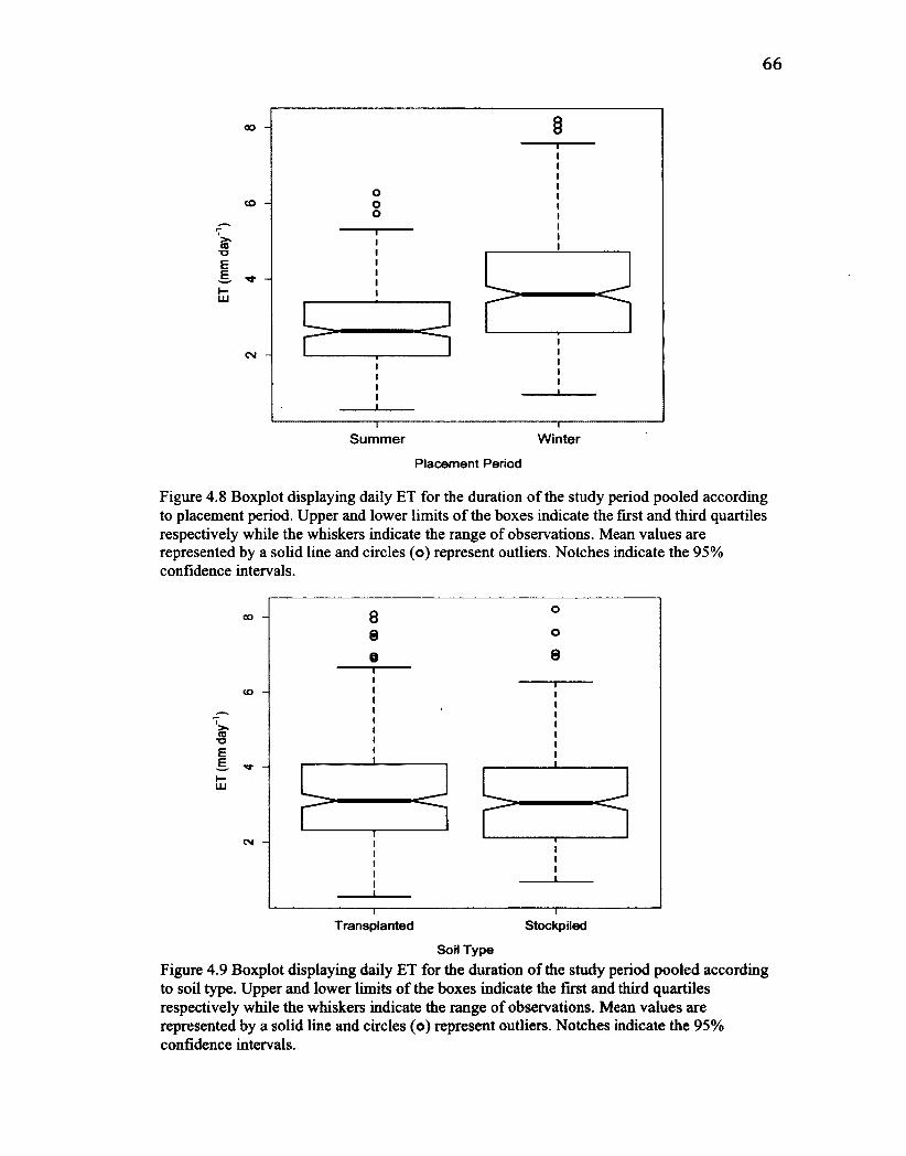
66
CO
<o -
>» CO "O E E
LU
<N
r •
Summer Winter
Placement Period
Figure 4.8 Boxplot displaying daily ET for the duration of the study period pooled according to placement period. Upper and lower limits of the boxes indicate the first and third quartiles respectively while the whiskers indicate the range of observations. Mean values are represented by a solid line and circles (o) represent outliers. Notches indicate the 95% confidence intervals.
CO -
CM -
i
<
J j <
i
>
i
3
Transplanted Stockpiled
Soil Type
Figure 4.9 Boxplot displaying daily ET for the duration of the study period pooled according to soil type. Upper and lower limits of the boxes indicate the first and third quartiles respectively while the whiskers indicate the range of observations. Mean values are represented by a solid line and circles (o) represent outliers. Notches indicate the 95% confidence intervals.
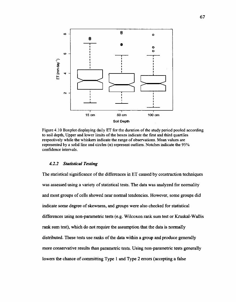
67
>» CD "O E £ H LU
15 cm 50 cm 100 cm
Soil Depth
Figure 4.10 Boxplot displaying daily ET for the duration of the study period pooled according to soil depth, Upper and lower limits of the boxes indicate the first and third quartiles respectively while the whiskers indicate the range of observations. Mean values are represented by a solid line and circles (o) represent outliers. Notches indicate the 95% confidence intervals.
4.2.2 Statistical Testing
The statistical significance of the differences in ET caused by construction techniques
was assessed using a variety of statistical tests. The data was analyzed for normality
and most groups of cells showed near normal tendencies. However, some groups did
indicate some degree of skewness, and groups were also checked for statistical
differences using non-parametric tests (e.g. Wilcoxon rank sum test or Kruskal-Wallis
rank sum test), which do not require the assumption that the data is normally
distributed. These tests use ranks of the data within a group and produce generally
more conservative results than parametric tests. Using non-parametric tests generally
lowers the chance of committing Type 1 and Type 2 errors (accepting a false

68
hypothesis or rejecting a true hypothesis). A summary of the findings is highlighted in
Table 4.2.
Table 4.2 Statistical significance test results for the effects of construction techniques on ET. Both parametric and non-parametric tests at the 95% confidence level were used. Only placement period resulted in significant differences in ET. Significant differences are indicated in bold.
Factor Wilcoxon Rank-Sum Test Kruskal-Wallis Rank-Sum Test
Placement Period W = 15896 n/a p-value <0.001
Soil Type W = 27369 n/a p-value = 0.25
Chi-squared = 6.88 Soil Depth n/a p-value <0.05
Placement period proved to be a statistically significant factor for ET at the
95% level. The Wilcoxon rank sum test confirms that cells constructed in winter have
consistently higher daily ET rates than those constructed in summer over the duration
of the study period. A possible explanation for this is that winter cells were visibly
more degraded, with less vegetation and more areas of open water.
In contrast, there were no significant differences between the cells of different
soil type. Cells filled with transplanted peat or stockpiled mixture had similar ET rates
(3.24 mm day"1 to 3.09 mm day"1 for peat and stockpiled respectively), even though
vegetation and irrigation regimes varied between the two construction techniques. The
high p value confirms that ET rates in cells of each of the two different soil types were
not significantly different.
To compare the three soil depth groups, an ANOVA based test in which the
difference of means can be tested for three or more groups was used. Again, because
the data showed some degree of non-normality, the non-parametric Kruskal-Wallis

69
rank sum test was used to assess statistical significance. The results indicated that there
was at least one significantly different daily ET in cells of different depths. However,
the p-value was relatively high ( p = 0.032) suggesting the significance may be low.
Because the Kruskal-Wallis rank sum test only indicated the presence of a significant
difference, and not which group is causing this difference, a pair wise matrix analysis,
in which each depth is compared to each other depth in one to one paired tests was also
performed. The results of this analysis are presented in Table 4.3.
Table 4.3 Pairwise difference of means and the associated Wilcoxon Rank Sum Test significance test results at the 95% level. Upper diagonal portion shows the actual difference in daily mean ET between the two depths while the lower diagonal section reports the corresponding p-value at the 95% significance level. Significant differences are indicated in bold.
15 cm 50 cm 100 cm 15 cm ^ -032 mm day"1 -038 mm day"1
50 cm ^ - +0.055 mm day"1
100 cm
Soil depth had a significant effect on ET but only for the shallowest cells (15
cm). The 15 cm deep cells had significantly higher daily ET rates compared to the
deeper 50 cm and 100 cm cells, while no significant difference was detected between
the two deepest soil depth groups (50 cm and 100 cm). Although the differences in ET
between the 15 cm cells and the two deeper ones were significant, the magnitude of the
difference is relatively small (0.32 - 0.38 mm day"1).
4.2.3 ET and Environmental Factors - Linear Regression and Correlation
To assess the relative influence of environmental factors in controlling variations in
ET, exploratory correlations were conducted for individual cell ET with incoming
solar radiation, VPD, wind speed, air temperature and water table depth. Figures 4.11
to 4.15 present scatter plots of mean daily ET against daily mean values of each
70
environmental variable. Linear regression lines and equations with associated
coefficients of determination (r2) are presented on the scatter plots for cells that had
significant relationships (95%, p<0.05).
Of all the environmental variables, incoming shortwave radiation showed the
strongest relationship with ET. All twelve cells had significant positive linear
regressions between ET and incoming solar radiation at the 95% level and had r2
values that ranged from 0.18 to 0.50 (Figure 4.11).
VPD and water table depth showed significant relationship with ET in only a
few cells (Figures 4.12 and 4.13 respectively). Three cells had a significant linear
regression between ET and VPD at the 95% level (W-S-15 cm, r2 = 0.12; S-P-50 cm,
r2 = 0.11; S-S-100 cm, r2 = 0.18). Two cells had a significant linear regression between
ET and water table depth, however the relationship was not in the direction that might
be expected; one cell had a negative relationship (S-P-100 cm, r2 = 0.21) while one had
a positive relationship (S-S-50 cm, r2 = 0.16). Presumably, increased VPD and a water
table depth near the surface should result in higher ET, however the linear
relationships between these individual variables and ET do not appear to be very
strong at this site. This lack of strong relationships of ET with water table depth and, to
a lesser extent, VPD is likely influenced by the irrigation regime. Having an excess of
water at the surface regardless of the environmental conditions may have created
heteroscedastic situation in which the connection between water availability at the
surface-atmosphere boundary and ET, was hidden by variability among other factors.

71
Wind speed and air temperature did not have any significant linear
relationships (95%) at the individual cell level (Figures 4.14 and 4.15 respectively).
Looking at the entire site pooled data (all cells) and using the more
conservative Spearman rank correlation test, ET was correlated with incoming
shortwave radiation (rs = 0.47) and to a lesser extent with the vapour pressure deficit
(rs - 0.23). Complete pooled data Spearman correlations are shown in Table 4.4. Water
table depth had little effect on ET (Not shown, all cell average rs = 0.12), again likely
because the cells were routinely watered and the water table was rarely much below
the surface of the cells. Wind speed and air temperature showed very weak correlations
with ET.
Table 4.4 A cell pooled data correlation matrix between ET and five controlling environmental factors with the top/right side of the matrix displaying the associated Spearman's rank correlation coefficient (rs) and the bottom/left displaying the corresponding p-value. Significant relationships are highlighted in bold. Also of note are the correlations between controlling factors themselves.
ET Shortwave Radiation
VPD Wind Air Speed Temperature
0.47 0.23 0.62
-.04 -.05 -.28 .02
-0.41 0.53 -0.25

72
TO TJ E „ E,
I— I I I CM
S-P-15cm
y= 0.009 x+0.45
[̂ =0.33 fK=0.05
S-P-50cm
y= 0.007 x+0.77
r*=0.26 p<=0.05
S-P-100cm
y= 0.009 x+0.75 ^=0.28 p<=0.05
#•.
S-S-15cm
y= 0.012 x+ 0.73
^=0.29 p<=0.05
S-S-50cm
y= 0.009 x+0.18 ^=0.32 p<=0.05
S-S-100cm
y= 0.015 x+-0.52
f*- 0.5 p<=0.05 •
W-P-15cm
y= 0.014 x+0.54
?= 0.27
W-P-50OT1
y= 0.01 x+ 1.58
r^- 0.18 p<=0.05 • • _•
W-P-100cm •
y* 0.013 x+ 1.04 • r*= 0.25 * p«0.05
W-S-15cm
y» 0.015 x+0.58 ^=0.33 p<*0.05
H
E o u>
W-S-50cm
y= 0.015 x+0.26 1^=0.29 p«0.05
E o o UO
W-S-100cm
y= 0.009 x+ 0.33 f*= 0.26 p<=0.05
E o o o
100 150 200 250 300 100 150 200 250 300 100 150 200 250 300 100 150 200 250 300
Mean Daily Shortwave Radiation (W m"2)
Figure 4.11 Scatter plots of ET and mean daily incoming shortwave radiation for each cell in the study. Correlations significant at the 95% level are shown.

73
to ~o E E
LLI ̂
S-P-15cm
• * • «.* *
• #C» •****• . • A ' , •
S-P-50cm
y= 0.765 x+ 1.81
1^=0.11 p<=0.05
S-P-100cm
• • •-
, : • '.* • -..ov • • •
S-S-15cm
• •
• •» <
^ • • •
S-S-50cm
. #
S-S-100cm
y= 1.778 x* 1.54
f^O.IS# p<=0 05
. «•! H •
W-P-15cm
• •
• % ••
W-P-50cm •
• •
, • w a
• •
• •
• * • # •
W-P-100cm
* * .•* • **
•V *•••
• • • • •
W-S-15OT
• • y» 1.518*+ 2.92
^=0.12 • • PJ=005 . •
E o m
W-S-50cm
• • • • • «. • E o o LO
W-S-100cm
* • • l i# • • + I
• # • • # • *
E o o o
i—i—i—i—i—i—i—n—i—i—i—i—i—i—n—i—i—i—i—i—i—n—i—i—i—i—i—i— 0.2 0.6 1.0 1.4 0.2 0.6 1.0 1.4 0.2 0.6 1.0 1.4 0.2 0.6 1.0 1.4
Mean Daily VPD
Figure 4.12 Scatter plots of ET and mean daily VPD for each cell in the study. Correlations significant at the 95% level are shown.

74
S-P-15cm S-S-15cm W-S-15cm
•••••
S-P-50cm S-S-50cm W-P-50cm W-S-50cm
>»
8.867 *+ 2.46 [*= 0.16 p<=0.05
o
00cm S-S-100cm W-P-100cm
-14.593*+ 4.2: r1- 0.21 p<=0.05
,v •
• • •
• •
-0.3 -0.1 0.1 -0.3 -0.1 0.1 -0.3 -0.1 0.1 4.3 -0.1 0.1
Mean Daily Water Table Depth (m)
Figure 4.13 Scatter plots by cell of water table depth to mean daily ET. Very little correlation was observed in any cell, likely due to consistent irrigation resulting in water rarely being a limiting component. Also, this situation may be heteroscedastic due to the influence of the irrigation regime and thus making the significance of any relationships questionable.
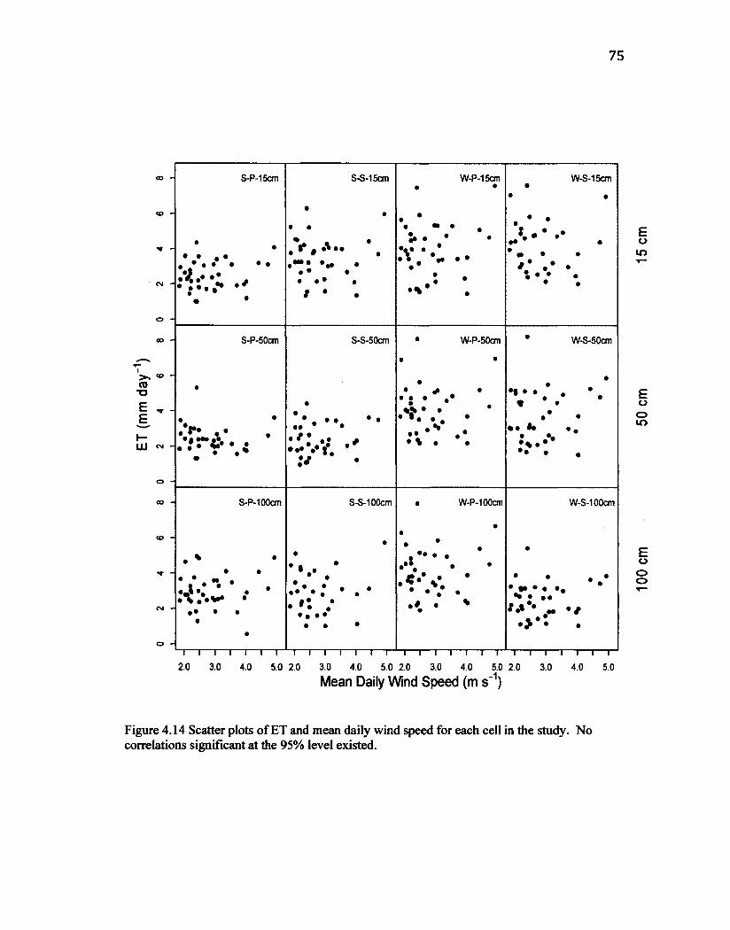
75
i >> <o ro
"CT E E
S-P-15cm
• • • • • • • *
* ••••- *'
S-P-50cm
>• . v r* . . .
S-P-100cm
• ' . - • t • •
A . • • • • •
S-S-15cm
• •
•—• • • • • • • • •
i • •
S-S-50cm
• •
• ' I • • *
S-S-100cm
* • • . •• • • * • «* •
• *• • •• •• • • •
W-P-15OT
• • •
• *
W-P-50cm
• + - • • • .» •*.V. . . . •* . • • * • i
W-P-100cm
W-S-15cm
•:• . • •
W-S-50cm
V - /
• • * *• ' * • ' ' • •
W-S-100cm
• • •• H 2 • •
** • •/
i—i—i—i—i—i—r*~i—i—i—i—i—i—I-^T—i—i—i—i—i—r^-i—i—i—i—i—i—r 2.0 3.0 4.0 5.0 2.0 3.0 4.0 5.0 2.0 3.0 4.0 5.0 2.0 3.0 4.0 5.0
Mean Daily Wind Speed (m s-1)
E o m
E o o ui
E o o o
Figure 4.14 Scatter plots of ET and mean daily wind speed for each cell in the study. No correlations significant at the 95% level existed.

76
S-P-15cm
• • • • r
\-V:-® A
S-S-15cm
•F» % • • .
•t •• . * •• • • I • * •
W-P-15cm • •
> * • • r .* • • u *
W-S-15cm
•• '«l
v •
S-P-50cm S-S-50cm W-P-50cm •
• •
W-S-50cm
> <o ra
TJ E , E,
I— I i I CM J % • • '•J. •* ••
». • •
• • •• •
f .
f.
• / v»
,» • a</
S-P-100cm S-S-100cm W-P-100cm • W-S-100cm
• ' . • • •
A « V *
• •»
• •
•••
• • «•
• •
Jk *• 1
r * *• v
S • • I*/ •
"T" 20 10 15 20
I
10 15 10 15
i
20
\
10 15
i 20
Mean Daily Air Temperature (C)
Figure 4.15 Scatter plots of ET and mean daily air temperature for each cell in the study. No correlations significant at the 95% level existed.

77
4 J Multiple Linear Regression Models
4.3.1 Initial models
The lack of strong correlations between ET and environmental factors presumed to be
controlling ET led to the creation of multiple linear regression models in order to 1)
help provide further insight into the controls on ET at the study site, and 2) gap fill
missing ET data for use in the water balance.
An individual multiple linear regression model was developed for each of the
12 cells in the study (Figure 4.16). Each model was initially constructed using cell
specific ET measurements and data for the five environmental variables. The models
were then trimmed according to AIC (Akaike's Information Criterion, section 3.3), by
removing the next insignificant variable that caused no additional reduction in
deviance. Also, the models attempted to adhere to the general n/g rule for the total
number of variables. A final model for each cell was composed of different total
numbers and combinations of variables, indicating the relative importance of different
environmental variables in cells of differing construction techniques.
4.3.2 Models with Interactions
Due to the lack of strong direct correlations among environmental variables, there is a
possibility that ET in the cells is controlled by a combination of the environmental
factors acting together. The nature of the interactions between groups of environmental
factors and ET is poorly understood (Souch et al. 1996; Drexler et al. 2004). It is
possible that models that consider these interactions amongst environmental variables
may be a more robust and accurate technique for gap filling and future prediction of

78
S-P-15cm / S-S-15cm / W-P-15cm / W-S-15cm /
JnftP 0 o/<b
00
•JyS °o
*jb
°Oi?o *
&&9 o
/ RMSE= 0.6213 / RMSE= 1.4029 / RMSE= 1.2707 / RMSE= 1.1475
S-P-50cni / S-S-50cm / W-P-50cm / W-S-50cm /
w°°
o wo£- o Qa
f" Ji&o' i °<fi fi-Wo o. -/> er
.• •Mo 0°
/ RMSE= 0.6354 / RMSE= 0.632 / RMSE= 0.974 / RMSE= 1.2284
S-P-100cm / S-S-100cm / W-P-100cm / W-S-100cm /
•̂0iWo°
o fS 5"'o oo ix--
•••••yS o°
"moo0
/ RMSE= 0.8067 / RMSE= 0.7848 / RMSE= 1.1574 / RMSE= 0.8272
0 2 4 6 8 0 2 4 6 8 0 2 4 6 8 0
Observed ET (mm day"1)
6 8
Figure 4.16 Observed ET plotted against predicted ET using a multiple linear regression model without interaction for each cell in die study. After models were trimmed for 95%, the majority ended up being very close to single linear regression models between shortwave radiation and ET.

ET. Therefore, the multiple regression models were re-designed to incorporate the
interactions by adding a term to the model representing the interaction between two or
more variables (Figure 4.17). The effect of including interactions in the models is
evident when comparing observed ET plotted against predicted ET for each cell with
and without interaction terms respectively (Figures 4.16 and 4.17).
The models without interaction terms became, in most cases, a linear
relationship between incoming solar radiation and ET after non-significant variables
were removed. This resulted in high RMSE values as models were biased, consistently
under-predicting ET. The performance of the simple linear regression models again
suggests the need to incorporate terms that represent two or more environmental
factors working together. The addition of interaction terms to the models greatly
improved the significance of the models and also reduced the RMSE. However, the
models tended to over-fit the data due to the number of significant terms, often not
satisfying AIC. The models with interactions often produced highly accurate
predictions of ET for the majority of the data, but also occasionally produced highly
unreasonable predictions of ET. These unreasonable outliers were typically
significantly under or over the range or potential ET values and often occurred in
situations of extreme values (high and low) of environmental factors. The inability to
keep predictions of ET near the range observed values at all times suggests that the
models were over-fit to the data.

80
S-P-15cm
RMSE= 0.1545 RMSE= 0.039
W-P-15cm
RMSE= 0.7355
W-S-15cm
tl'8
o _
o
RMSE= 0.9142
S-P-50cm
RMSE= 0.0227
S-S-50cm W-P-50cm
RMSE= 0.1249
W-S-50cm
RMSE= 0.5238 RMSE= 0.5418
S-P-100cm
RMSE= 0.3546
S-S-100cm W-P-100cm
RMSE= 0.4533
W-S-100cm
RMSE= 0.5184
1 1 1 1 n 1 1 1 n 1 1 1 rr 0 2 4 6 8 0 2 4 6 8 0 2 4 6 8 0
Observed ET (mm day"1)
RMSE= 0.2769
1 I I r 2 4 6 8
Figure 4.17 Observed ET plotted against predicted ET using a multiple linear regression model with interaction terms, for each cell in the study. Models were often over-fit, and produced outliers so unreasonable they cannot be shown in figures.

81
The over-fitting of the models is primarily due to the low number of observations of
ET for certain cells (n~40). However, when data was pooled to increase the number of
observations (i.e. by construction technique or all cells together), the tendency of the
models with interactions to over-fit the data decreased. Often this came at the expense
of lower correlation coefficients and higher RMSE values, but overall the models
performed reasonably well. An example of one such model is shown in Table 4.5 with
its associated plot of predicted ET against observed ET in Figure 4.18.
Table 4.5 All cell pooled multiple linear regression model terms, estimates of their coefficients, and associated p-values. The models overall adjusted r2 value is 0.4235 with a p-value of 2.2e"16. In this table, Wdspd is wind speed, Kdown is incoming shortwave radiation, Temp is air temperature, Wtd is the water table depth and VPD is the vapour pressure deficit.
Model Term p-value Kdown Wdspd Temp
Wtd
3.1e"14
3.3e 1.3e"05
.-13
0.019 Wdspd+Kdown Kdown+VPD Temp+VPD
Wdspd+Temp Kdown+Temp
-16
W dpsd+Kdown+T emp W dspd+Kdown+VPD
W dspd+T emp+VPD

82
oo -
7 <o >. (0 TJ
(N -
O O o CD O O Qa,
. - - •d
§
sn.
o&?
o <p o 0
RMSE= 0.9923
T
6
T"
8
Predicted ET (mm day"1)
Figure 4.18 All cell pooled data plot of Observed ET against predicted ET using a multiple linear regression model with interaction terms. Model contained 12 variables, easily satisfying the n/3 general rule and AIC test, resulting in a model able to predict ET based on the five controlling factors without over-fitting.

4.4 Recursive Partitioning - Tree Models
As mentioned previously (Section 3.4), recursive partition models or "trees" differ
from multiple regression models in that data is broken up according to specific
thresholds of explanatory variables that result in the least amount of deviance
(Crawley, 2005). This technique offers the potential to include interactions between
variables, but also the thresholds at which those variables may become important. In
contrast to the multiple linear regression models, recursive partitioning models may be
capable of predicting ET without a strong tendency to over-fit data (Crawley, 2005).
The tree method provided a highly effective, visual way to determine which
environmental variables were most responsible in controlling ET and the important
thresholds related to their connection with ET. The pooled all cell tree model is shown
in Figure 4.19 with its predicted ET plotted against observed ET shown in Figure 4.20.
Because the tree models were less influenced by low numbers of observations,
they generally did not over-fit the data. The tree models typically had a slightly higher
RMSE for large pooled data groups than the multiple linear regression models.
However, the tree models provided reasonable estimates of ET far more often, with
only very few predictions deemed to be outliers. Figure 4.21 displays the individual
cell tree model predicted ET plotted against observed ET for the 12 study cells.
Comparing the effectiveness of the tree models with the multiple linear regression
models with interaction terms (Figure 4.17), it is evident that although the tree models
have more dispersion in the data, the lack of extreme outliers results in a very similar
RMSE. The ability of the tree models to consistently produce accurate and reasonable
predictions of ET is a major advantage over multiple linear regression models.
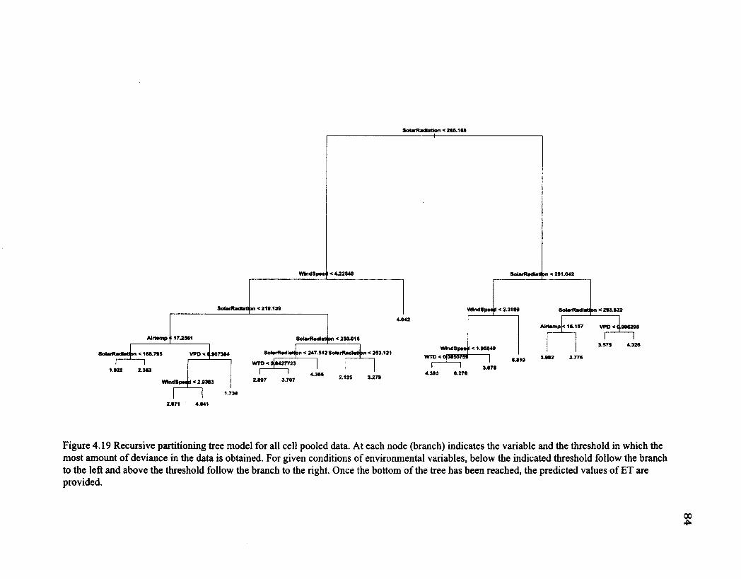
SoiarRadlatfon < 269.158 1
WtndSp** I < 4^2546 SolarfUdtotl >n < 281.042
Alftemp
SotavRadlatJ m < 218.139
17.2561
SoterfUdteti mi < 168.785
1.822 2.383
VPD < < .807384
SolarRadtatl < 250.016
Sc4«rR*dl*ti >n < 247.512 SotarfUdiatl mi < 253.121
< 2.3108
.85848
WTD < 010427723
2.887 3.707 2.135 3.278
WlndSpM I < 1.!
WTD < 0)6856759 1
| 1 1 1 1 3.878 4.383 6.270
SolarRadiati >n < 283.832
Aktomp < 16.157 VPD<(.885285
3.575 4.326
3.882 2.775
2.871 4.041
Figure 4.19 Recursive partitioning tree model for all cell pooled data. At each node (branch) indicates the variable and the threshold in which the most amount of deviance in the data is obtained. For given conditions of environmental variables, below the indicated threshold follow the branch to the left and above the threshold follow the branch to the right. Once the bottom of the tree has been reached, the predicted values of ET are provided.
oo
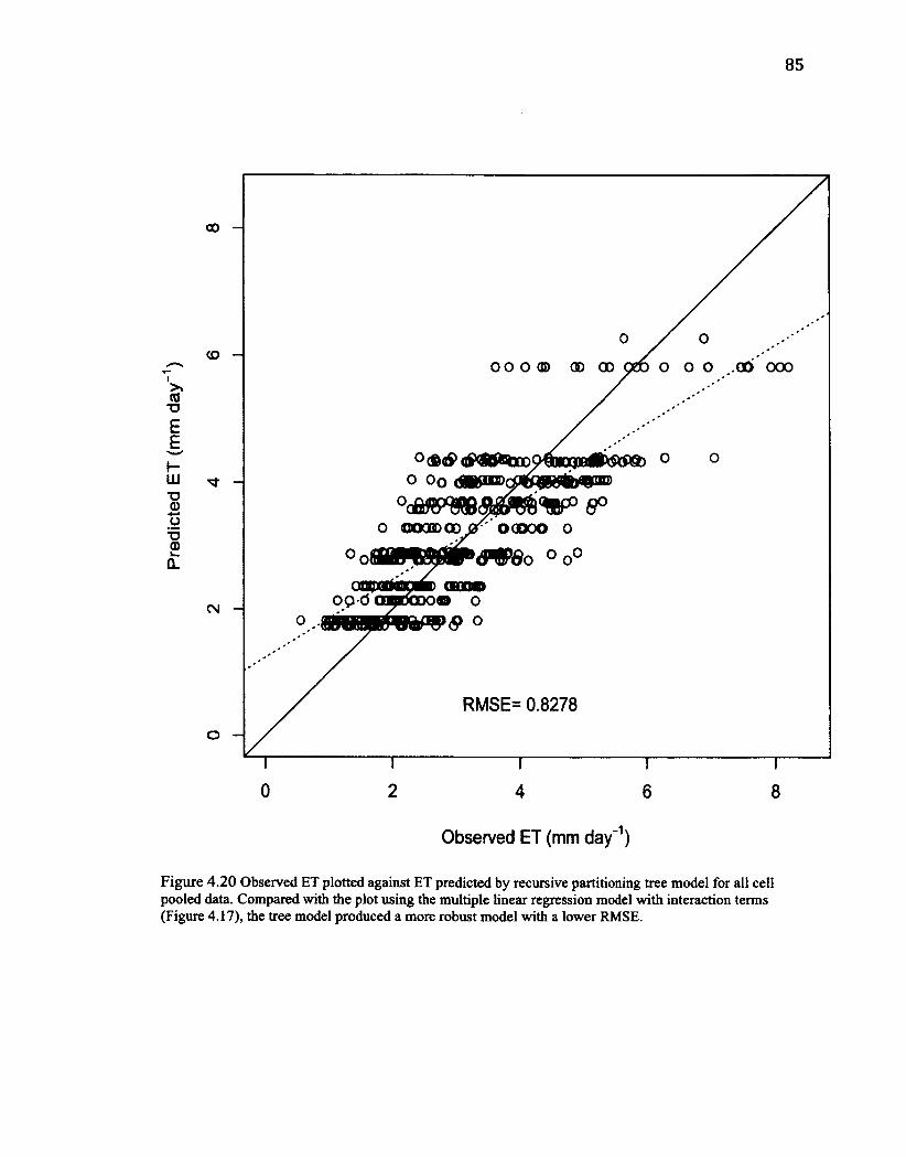
85
RMSE= 0.8278
Observed ET (mm day"1)
Figure 4.20 Observed ET plotted against ET predicted by recursive partitioning tree model for all cell pooled data. Compared with the plot using the multiple linear regression model with interaction terms (Figure 4.17), the tree model produced a more robust model with a lower RMSE.
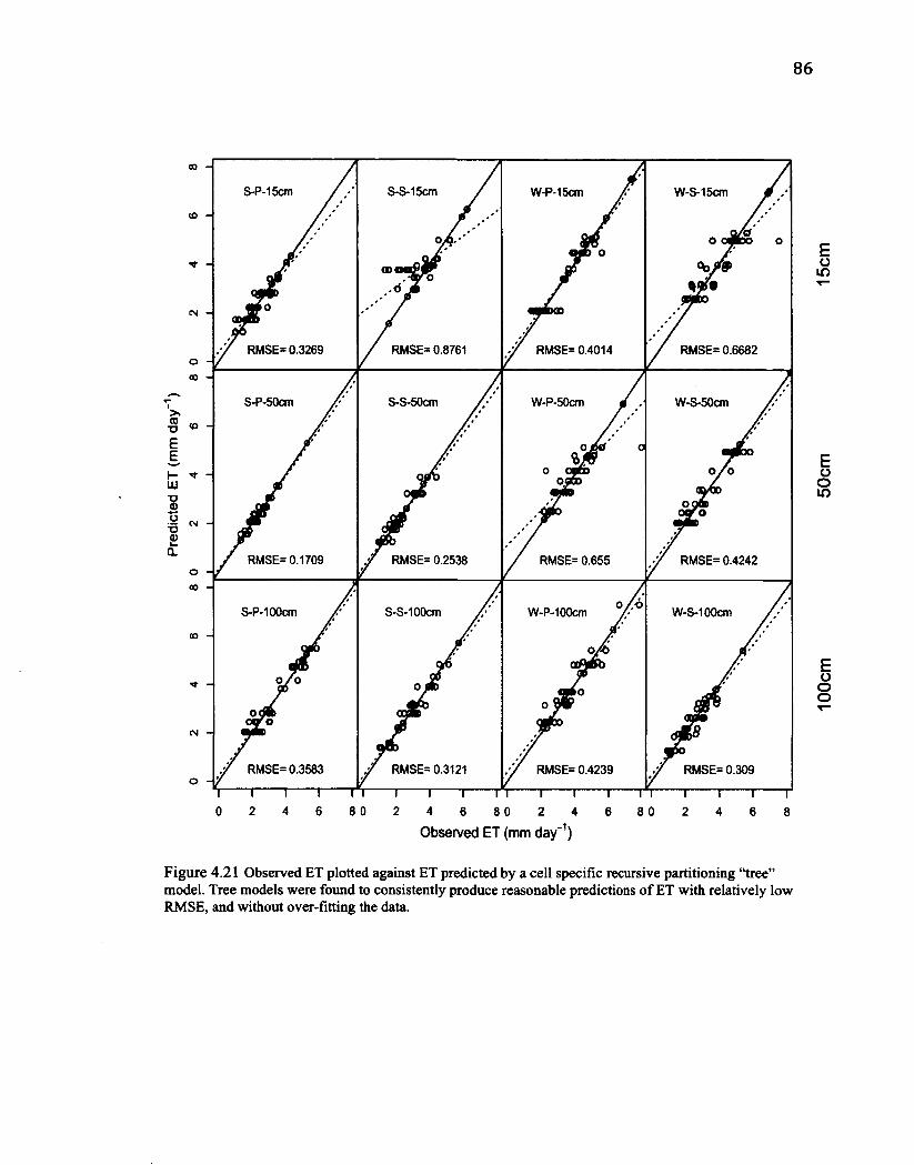
86
S-P-15cm
RMSE= 0.3269 RMSE= 0.8761
W-P-15cm
RMSE= 0.4014
W-S-15cm
RMSE= 0.6682
S-P-50cm
RMSE= 0.1709
S-S-50cm W-P-50cm
RMSE= 0.2538
W-S-50cm
RMSE= 0.655 RMSE= 0.4242
S-P-100cm
o -'/ RMSE= 0.3583
S-S-100cm W-P-100cm
RMSE= 0.3121
W-S-100cm
RMSE= 0.4239
i 1 1 1 n 1 1 1 n 1 1 1—n 0 2 4 6 8 0 2 4 6 8 0 2 4 6 8 0
Observed ET (mm day"1)
RMSE= 0.309
Figure 4.21 Observed ET plotted against ET predicted by a cell specific recursive partitioning "tree" model. Tree models were found to consistently produce reasonable predictions of ET with relatively low RMSE, and without over-fitting the data.

87
4.5 Cell Water Balances
4.5.1 Inputs and Outputs
Water balances were calculated for each of the 12 cells in the study, according
to equation 2.3. Inputs comprised the irrigation totals for each cell along with the
precipitation at the site (Figure 4.22). These totals ranged from ~ 200 mm to -475 mm,
with June accounting for the bulk of the inputs for most cells. The hot, dry weather led
to very high irrigation volumes and subsequently high inputs, even with very little
precipitation. The apparent great variation in input depth suggests that some cell liners
may have leaked.
500 -|
400 -
„ 300 -
(0 3 a ~ 200 -
100 -
0 J
Figure 4.22 Water balance inputs organized by month for each cell for the duration of the study period.
• June Irrigation
• June Precipitation
• July Irrigation
•I July Precipitation
• August Irrigation
CZ1 August Precipitation
i i i § i in in in in o E E 5 o o o o o o in m m
£ o o o £ o o o
£ o o o CO CO CO CO
CO CO § § CO CO «> a. co • i CO CO
£ o o 0 1 CO

Outputs for the cells were assumed to be entirely of losses through ET.
However, due to logistical and environmental constraints, ET could not be measured
every day. Therefore, in order to obtain a more accurate estimation of cell outputs,
missing data was gap filled with ET predicted by the recursive partitioning tree model
(Section 4.4) specific to each cell. Tree models were chosen because they did not over
fit the data and produce extreme outliers. Figure 4.24 displays the outputs comprised
of measured ET and gap filled model predicted ET.
Overall, output (ET) totals in the cells displayed a similar amount of
variability as the inputs did. Outputs ranged from -175 mm to ~325 mm. As
mentioned, June had many relatively high ET days and so comprised the bulk of the
outputs for the majority of cells. July totals were slightly less than June, perhaps due to
more days with precipitation events. ET slowed down notably towards the end of the
growing season, reflected in the much lower output totals for August. These large
differences in output totals amongst cells can likely be attributed to differences in
construction techniques (treatments).

89
350 -|
300 -
250
| 200
3 Q. 3 O 150 -
100
50 -
0 -1
• June ET • July ET • August ET
E E E o o o in in » •L co a.
E & T— I CO
E E o o O O O O Q O in in in in o o CO
E E E E o o o o — - - o o CO
E o o o
M W ^ J l O W J g CL CO CO CO
o. co I I
$ §
Figure 4.23 Water balance outputs (ET) arranged by month using recursive partitioning model gap filled data for each cell for the duration of the study period.
4.5.2 Cumulative Water Balances - 2010 Growing Season
Cumulative water balances were calculated to track the progression of inputs
and outputs and the change in water storage of the cells (Figure 4.25). Comparison of
inputs and outputs with the actual change in storage (water table change multiplied by
the specific yield) acts as a check to the predicted change in water storage. By
comparing inputs and outputs, an estimate of the magnitude of the water balance and
its components can be made and differences and similarities between cells can be
analyzed and perhaps attributed to specific construction techniques.

90
© © H CM
S-P-15cm S-S-15cm W-P-15cm W-S-15cm
S-P-50cm
o -
W-P-50cm W-S-SOcm
o * 1 S-P-100cm S-S-100cm
o -
W-P-100cm W-S-100cm
I— 160
T— 160
DOY
-i— 160 200 160 200 200 200
Legend Inputs (Irrigation + Precipitation)
Outputs (ET)
Predicted CIS
Actual CIS
Figure 4.24 Cumulative water balance plots for each cell in the study. Outputs are composed of directly measured ET and gap filled ET determined using a cell specific recursive partition (tree) model. Blue lines indicate inputs, red lines indicate outputs, green lines represent the predicted change in storage, while black lines represent the actual change in storage.

91
Half of the cells were estimated to have experienced a very small change in
water storage as inputs and outputs were very similar; this was supported quite closely
by the change in the water table depth. Six cells (S-S-15 cm, W-P-15 cm, W-S-15 cm,
S-P-50 cm, W-P-50 cm, S-P-100 cm) exhibited a predicted change in storage very near
to that of the actual change in storage (Table 4.6). Differences between these cells
were relatively small, ranging from 35 mm (W-P-50 cm) to as low as 11 mm (W-S-15
cm), and so should be considered as reasonable estimates of the overall water balance
in these cells.
Table 4.6 Summary of predicted and actual change in water for storage for each of the cells at the end of the study period. The relative difference between these two terms is a good indication of water balance accuracy and/or the presence of leaking cells.
Cell Predicted Change In Storage (mm)
Actual Change in Storage (mm)
Difference (mm)
S-P-15 cm 35
CO o 1 138
S-S-15 cm -10 -28 18 W-P-15cm 6 -9 15 W-S-15cm 21 9 11 S-P-50 cm -44 -24 19 S-S-50 cm 307 40 267 W-P-50 cm -32 3 35 W-S-50 cm 93 5 88 S-P-100 cm -40 -6 34 S-S-100 cm 238 -15 253 W-P-100 cm 36 -25 60 W-S-100 cm 126 -21 147
Three cells produced cumulative water balances with large differences in
predicted change compared to actual change in water storage. These three cells (S-P-
15 cm, W-S-50 cm, W-P-100 cm) had discrepancies greater than those of the first
group, 138 mm, 88 mm and 60 mm respectively (Table 4.6). These differences in the

cumulative water balance are large enough to suggest a potential measurement issue
but not so large to indicate a major technical or logistical problem with the cells.
Based on the water balance estimates, three cells (S-S-50 cm, S-S-100 cm, W-
S-100 cm) would have had a large gain in storage yet, based on actual changes in the
water table, true storage change was much less. The summer placement, stockpiled
mixture cells of 50 cm and 100 cm were estimated to have had nearly twice as much
inputs as output, a surplus of close to 200 mm (Figure 4.24). This difference between
inputs and outputs was not supported by the actual change in storage, which in both
cases remained very close to 0, or by visual confirmation of any significant water level
change. The presence of such a large discrepancy may be a strong indication that the
liners in these cells were leaking significant amounts of water. Approximate water
depth leakage estimates for these three cells are substantial at -3.4 mm day'1 (102 L), -
1.9 mm day"1 (57 L), and -2.9 mm day"1 (87 L) for S-S-50 cm, S-S-100 cm, and W-S-
100 cm cells, respectively.

5.0 Discussion
5.1 The Problem
Most of the oil sands mining areas are located near the southern fringe of the Boreal
biome. This ecosystem is typically composed of vast areas of forests, forested
wetlands, bogs, fens and swamps. With regards to ecosystem reclamation related to oil
sands mining, upland forest systems have been established in the region with some
degree of success. However, little work has been undertaken on designing and
establishing important lowland ecosystems that maintain saturated conditions and
wetland vegetation.
Reclaiming and constructing wetlands after mining presents many challenges.
Topography must be created in some way as to reflect the natural landscapes while
controlling for erosion and stability. Soil material must be salvaged during mining and
later placed atop reclamation surfaces, resulting in a profile that is considerably altered
compared to the pre-mining landscape. The climate of the region is cold, with a short
growing season that limits vegetation growth. Furthermore, the region around Fort
McMurray relatively dry, placing limits on vegetation and presenting a challenge in
maintaining moist conditions required for wetland systems.
5.2 The Cells
In an attempt to evaluate techniques to construct large-scale wetland systems,
Syncrude Canada Ltd created a series of test plots (the U-shaped cells), 12 of which
were studied for this thesis. The cells were designed to behave similarly to natural
boreal wetlands (bogs), by adding liners to limit deep percolation and lateral flow, and

thus confining the majority of exchanges to those between the surface and the
atmosphere. However, unlike natural wetlands, water was added via irrigation to
maintain conditions suitable vegetation establishment. Because of the irrigation, the
cells had a distinct hydrological difference compared with natural wetlands, which
must be acknowledged when considering the implications of study results.
Each cell investigated was unique due to the combination of three construction
strategies (soil/vegetation type, soil depth, and soil placement period). There were
large visible differences among the cells; some were lush with green vegetation while
others contained very little live vegetation with areas of exposed degrading organic
material. Invasive vegetation (grasses and cattails) was predominant in some cells,
whereas others largely consisted of native species. Hydrologically, some cells had
ponded water for the bulk of the growing season, whereas others were comparably dry.
The combinations of construction techniques are directly responsible for these
differences, which strongly impacted cell water balances.
5.3 Controlling Factors on ET
Due to the presence of liners in all cells, ET was the dominant loss of water and
became the central focus of this study as water management of future wetlands will be
largely controlled by surface-atmosphere coupling. It is unclear whether test-scale
wetland plots respond to the same environmental drivers as natural wetlands and
whether results from this study can be scaled up to larger wetlands. Regardless,
understanding the relative influence of placement strategy on ET will provide a first-

order estimate of how management techniques can affect water losses to the
atmosphere.
ET varied spatially and temporally at the study site. Highest ET rates were
observed at the beginning of the study period in early June, were generally steady in
July and began to decrease in August (Figures 4.5 and 4.6). Using the Penman-
Monteith framework, the fluctuation of ET throughout the study period was considered
to be controlled by five environmental factors: incoming solar radiation (a surrogate
for available energy), VPD, air temperature, wind speed (turbulence), and water table
depth.
Preliminary attempts to assess the relative influence of each of the five
environmental variables on ET using linear regression provided generally weak
relationships. Linear regression modeling suggested ET was mainly driven by
incoming solar radiation, which was the only variable significantly related to ET
(Figure 4.11 and Table 4.4). Previous studies in wetlands also found ET to
predominantly driven by radiative energy (Humphreys et al. 2006; and Kellner, 2001);
however the relationship at the cells was considerably weaker (r = 0.47 for pooled
data) than previous studies. The other environmental variables exhibited few
significant relationships with ET (Figures 4.12 through 4.15).
5.3.1 Multiple Linear Regression Models
To explore the complex interactions among environmental variables that may act to
control ET, multiple linear regression models were created. Initial multiple linear
regression analysis considered the additive effects of each individual environmental
variables operating at the same time. Generally, these models were able to provide

improved correlations with ET than the simple one-to-one regression equations.
However, after insignificant (p>0.05) variables were removed, many of the resulting
models were reduced to the original one-to-one relationships between incoming solar
radiation and ET. The inability of the multiple linear regression models to explain ET
using only additive individual relationships between environmental variables and ET
suggested that complex interactions among variables are important.
The addition of interaction terms to the multiple linear regression models
greatly improved the ability to explain ET. Substantial increases in correlation were
observed with coefficients of determination (r2) as high as -0.98 and RMSE values as
low as -0.023 (Figure 4.17). In many cases, individual variables did not have a
significant relationship with ET, but new variables created that were composed of two
or more previously insignificant variables exhibited significant relationships with ET.
Many of the interaction terms were considered significant, and new models contained
a far greater number of variables than the previous ones. Also, each new model was
composed of a unique combination of individual and/or interaction terms reflecting the
complex nature of the relationship between the environmental variables and ET.
Because the new models were considerably more complex, uncertainty existed in their
ability to explain data and predict ET and gap fill missing data. Curiously, some
models contained nearly as many significant terms as data points - surpassing
statistical considerations and resulting in the possibility of over-fitting the data.
Consequently, some models were susceptible to producing extreme outliers, and were
assumed to be poor at gap-filling ET on days with no observations. While some
models produced reasonable gap filled data, the production of extreme outliers resulted

in water balance estimates that were highly biased, reducing the credibility of this
method for interpolation data.
Multiple regression models that used pooled data from the cells reduced the
tendency to over-fit the data due to higher numbers of observations and a reduction in
the number of significant terms. However the reduction in complexity came at the cost
of a reduction in the strength of the correlations and of increases to the RMSE. The
tendency of multiple linear regression models to over-fit the data is likely amplified in
small data groups and/or when predicting ET for small data groups where limited
observations exist for calibration (e.g. rainy days).
Results from the multiple regression modeling suggest that the interactions
between any two or more of the five controlling environmental variables explain more
of the variability in ET than the sum of the individual relationships of those same
variables with ET. While mediocre at gap-filling, the models do provide some
indication of which interaction variables (two or more environmental variables
working concurrently) play an important role in controlling ET as this site.
5.3.2 Recursive Partitioning Models
Recursive partitioning models implicitly include interactions between
environmental variables. Any numerical model output is a result of a series of
decisions at nodes along the branches of the tree. Because most outputs are a result of
different variables at each node, the potential for interaction between variables is
created in the model. In addition, the inclusion of thresholds identifies not only
potentially important interactions but also the range of values under which these
interactions become important.

Recursive partitioning models were better at predicting and thus more useful
for gap filling. Because tree models work with branches containing specific variables
and threshold values, predictions are stratified and change by fixed intervals to as input
variables change. This stratification occurs as predictions for situations of similar
environmental conditions often result in the same value of ET. However, this tendency
to produce tiered predictions of ET keeps the models from over-fitting the data and
reduces their propensity to generate extreme outliers.
By analyzing the recursive partitioning models, it was possible to identify
important environmental factors and important interactions on controlling ET. Solar
radiation was the most important individual variable, as shown by the number of times
it is repeated in the models. Additionally, these models reveal other environmental
factors that become important depending on the value of solar radiation. For example,
in many cases wind speed and, to a lesser extent air temperature, became important
explanatory variables during times of relatively low solar radiation. Conversely, VPD
was often important during periods of high solar radiation. Other similar dependencies
between environmental variables appear further down the tree; however they may be
less significant. The recurrence of these patterns throughout many of the models
underscores the potential that interactions between environmental variables have
significant influence on ET.
Future analysis using recursive partitioning could focus on the value and
composition of threshold values that work to control the complex process of northern
wetland ET. Tree models show promise in helping to identify the dominant controls,
and their thresholds values at specific sites and may hold the potential to be expanded

over large areas when used in combination with remote sensing techniques. However,
tree models are often not optimal upon creation and so further study should also
consider validation techniques such as bootstrapping and random forest analysis.
5.4 Effects of Treatments
Placement period of the soil and, to a lesser extent, the depth of soil medium
significantly affected ET. Winter placement cells had higher growing season ET rates
than summer placement which is likely explained by the nature of the soil medium,
particularly for live transplanted peat. During winter installation, soils were frozen and
moved in a series of blocks from the disturbed wetland or stockpiled storage area.
These frozen soils had a tendency to fracture upon placement, degrading the overall
soil structure and creating large cracks at the surface throughout the cells, which were
then filled with loose peat. The impact of these fractures became apparent in the
following spring during thaw when cracks became preferential pathways for
channelization and erosion, redistributing loose decomposed organic material to the
cell edges. As the growing season progressed, degraded material throughout the cells
remained wet after continual irrigation due to its greater near-surface storage capacity,
enhancing evaporation. This process was more pronounced in the shallow cells where
the surface peat and vegetation had dies and degradation was considerable. As soils
were artificially irrigated, degraded cells were much wetter near the surface and ET
was enhanced.
Soil depth also influenced ET rates and the water balance. The shallowest cells
(15 cm) had significantly higher ET than the 50 cm and 100 cm cells. However, these

100
deeper cells did not display significant differences in ET with each other. Given that
only the 15 cm depth cells were significantly different, it is possible that there is a
depth threshold, beyond which the placement depth has limited influence on ET.
Shallower soil cells (S-P-15 cm, S-S-15 cm, W-P-15 cm, W-S-15 cm) were prone to
flooding during irrigation or rain events, and often had free water at the surface that
enhanced ET. Deeper soils provided for increased storage, reducing the frequency of
ponding compared with the shallower cells. Additionally, vegetation in the shallow
cells was often dead or dying, due to disturbances to its rooting zone upon transplant.
However, transpiration was likely small compared with evaporation due to the cells
near continually-saturated conditions.
There were no significant differences in ET based on soil type (stockpiled
mixture vs. live peat transplant). While there were strong visual differences between
live and stockpiled mixture cells in terms of plant species, there were no significant
differences despite stockpiled soil mixture cells having much greater LAI's.
The implication of these results on future reclamation techniques is important,
as future wetland construction projects, in some cases, have actively managed water
use systems that provide water to the wetland during initial stages of development.
Management of freshwater resources in northern Alberta is of great importance as it
relates to mining, and any opportunity for a reduction in freshwater use is significant.
Construction techniques that reduce ET rates, such as deeper soil placements, have the
potential for long-term savings in water use despite higher initial placement costs
associated with the movement of more material.

From this research, it is not possible to evaluate the long-term sustainability of
wetland placement techniques due to the highly managed nature of the cells. It is
unclear how keeping the cells at near-saturation impacts their long term performance,
and also masks the true evaporative dynamics associated with lowering water tables in
organic soils (Nicholas and Brown, 1980; Ingram, 1983; Lafleur et al. 2005). Future
research at the cells may assess how ET varies under conditions where cells are not
artificially watered, and how vegetation change is linked to water balance components.
From the water balances, four cells (S-P-15 cm, S-S-50 cm, W-S-100 cm, S-S-
100 cm) appear to have leakages through the cell base, which is likely due to degraded
liners. Cracks and punctures in geosynthetic liners are generally related to installation
techniques and degradation over time. Natural wetlands in the boreal region typically
form above impermeable clay soils, and comparison of water balances between leaking
and non-leaking cells leads to equivocal conclusions based on the extra water applied
to the leaking systems.
5.5 Context - Comparison with Other Natural and Constructed Sites
Despite being a pilot study to assess the effect of construction techniques on the water
balance (and vegetation/carbon dynamics not discussed in this thesis), it is clear that
the cells are distinct from natural wetlands in terms of size, setting, physical properties
and hydrology through the irrigation regime. Regardless, the comparative nature of
this study does allow construction techniques such as soil depth and placement
strategy to be assessed.

Table 5.1 summarizes the relative growing season ET rates based on
construction technique whereas Table 5.2 summarizes values presented in the literature
for undisturbed boreal and constructed wetlands. Placement period was the greatest
factor that distinguished ET among the cells, and was greater than ET rates reported in
the literature for other wetlands in similar regions. This is an important consideration;
that soil placement period may be the most important factor in controlling water
balance dynamics by strongly affecting soil properties (which in general are more
degraded in winter cells). ET rates from these cells approach those more typically
found in southern climates, although it must be noted again that cells were maintained
artificially wet.
Table 5.1 Summary of ET rates according to construction techniques that caused statistically significant differences. Data reported are mean and maximum values for the 2010 growing season.
Construction Technique Mean ET Rate Maximum ET Rate (mm day"1) (mm day"1)
All Cell Pooled 3.2 8.2 Winter Placement Cells 3.6 8.2
Summer Placement Cells 2.7 6.3 15 cm Soil Depth Cells 3.4 7.6
Pooled 50 and 100 cm Soil Depth Cells 3.0 8.2

103
Table 5.2 Summary of ET rates from previous wetland studies. Data are reported mean and maximum values for the growing season period. Wetland type is as reported by the authors, (adapted from Lafleur et al. 2005)
Study Wetland Type Location Mean ET (mm day'1)
Maximum ET (mm day'1)
Lafleur Natural rich fen James Bay, Ontario 2.9 5.0-6.0a
(1990) sedge dominated (51°07' N, 79°51'W)
Lafleur and Natural poor fen Hudson's Bay 2.5 n/a Roulet sphagnum Lowlands, Ontario (1992) dominated (50°20' N, 80°05* W)
Moore et al. Natural rich Fen Schefferville, Quebec 2.7b n/a (1994) sphagnum/sedge (54° 52' N, 66° 40* W)
dominated Price (1996) Disturbed limited Toubiere Fafard 2.9 5.0-5.5a
sphagnum cover Peatland. Quebec (48047*N, 72°10'W)
Lafleur et al. Natural Poor Fen BOREAS northern 1.8b n/a (1997) sedge/tamarack study area, Manitoba
dominated (55.9°N, 98.4°W)
Joiner et al. Natural Poor Fen BOREAS northern n/a 3.0-3.5a
(1999) sedge/tamarack study area, Manitoba dominated (55.9°N, 98.4°W)
Lott and Constructed Monroe County, 3.5 6.0-6.5a
Hunt (2001) shrub/sedge Wisconsin dominated (43.29°N, 90.83°W)
Van Seters Disturbed Cacouna Peatland 2.9 6.0-6.5a
and Price limited sphagnum Quebec (2001) cover (47°53'N, 69°27'W)
Petrone et al. Restored Fen Bois-des-Bel n/a 4.5-5.0a
(2001) sphagnum/straw Peatland, Quebec mulch (47° 53'N, 69° 27'W)
Lafleur et al. Natural Bog Mer Blue Bog, 2.2 - 3.3C 4.0-5.0 (2005) shrub covered Ontario
(45.40°N, 75.50 °W)
Raddatz et Natural Poor Fen Churchill Tundra n/a 3.0-3.5 al. (2009) sedge dominated Sedge Fen, Manitoba
(58°40' N, 93°50' W) a estimated from figure b computed from seasonal total ET 0 Range of values from more than one year of observations

104
The shallowest cells (15cm) had a slightly higher mean ET rates, whereas the
deeper soil depths (50 cm and 100cm) had higher maximum ET rates. Mean ET in the
15 cm cells still fell within the range of values observed in previous studies, but they
were closer to the upper range likely due to wetter than normal conditions. Maximum
ET was also higher than previously reported.
Mean ET at the site was generally within the range of values found in
comparable wetlands, although at the upper range. At times ET exceeded values
reported elsewhere. Again, the relatively high ET, particularly maximum rates, are
influenced by many factors including the maintenance of saturated conditions, altered
soil/vegetation properties, and a potential "oasis" effect caused by the cells being
surrounded by relatively dry mine soils. While direct comparison is difficult, Roulet et
al. (1997) and Lafleur (2008) suggest that bogs and poor fens should have relatively
low ET rates compared to other wetland types. In contrast, construction techniques and
management practices indicate that these cells are hydrologically distinct from the
natural systems they were designed to replicate.
5.6 Implications for Future Research
The results of this research have implications for the understanding of how ET is
controlled in northern wetlands, the relationship between wetland construction
technique and ET, and subsequently, the hydrologic behaviour of these constructed
wetlands. This understanding should contribute to the long-term success of future
reclamation and/or construction of wetlands in relation to oil sands mining. Further
study with technical improvements and more complex modeling could lead to more

accurate results and thus create a better understanding of the processes involved in
controlling ET. Several suggestions to improve future studies are identified below.
Number of Observations
The number of ET measurements should be increased. The low number of
measurements in this study increased uncertainty in the results and created problems
when performing statistical testing and empirical modeling. An increase in the number
of observations would increase data robustness, improve models and help guide
recommendations with more confidence. This is especially true for situations of low
ET (inclement weather), as models tended to have difficulty in these situations given
the lack of calibration data points.
Increased Sample Variability
Future studies at this site would benefit from diversifying the measurement locations
within the cells to find more representative locations. The cells in this study contained
only one measurement location (lysimeter) and its location was determined by space
availability and/or its proximity to the board walks (accessibility). Increasing the
diversity of measurement locations would help ensure that observations are truly
representative of each cell as a whole.
Statistical Models vs Physical Models
Physically based models (Penman-Monteith) often have a difficult time operating at
scales as small as the cells and would have required cell specific measurements of
every input variable. In the past, statistical models were often unable to incorporate
complex physical processes - the foundations of physically based models. However,
this study has shown that specific multivariate statistical modeling approaches can, in

fact, identify complex interactions on the micro-scale and without the need for more
complicated and expensive data collection. Future studies could compare the these
newer multivariate statistical models with physically based models with in order to
establish if the complex interactions revealed by these models hold any physical
foundations in known scientific processes. If this calibration is successful statistical
models such as the multiple linear regression models used in this study could be fit to
different land surface types and then used to estimate/model ET over large areas where
measurements are not available
Irrigation and Water Table Effects
In this study, all cells were watered so extensively that water tables rarely fell much
below the surface. Future studies should focus on quantifying irrigation volumes and
determining the effects of irrigation regimes given their possible impact on the
sustainability of wetlands once they have been constructed. For example, future
research could attempt to establish the effect of lower, more natural water tables that
experience greater fluctuations than those in this study. This could be achieved through
pairing cells of the same construction technique and providing regular irrigation to one
and only periodic irrigation to the other. A better understanding of how the cells
respond to drier conditions could help increase the success of constructed wetlands and
even determine a minimum water table threshold. Such a threshold could likely save
vast quantities of water.

6.0 Conclusions
Oil sands mining can be particularly destructive to terrestrial ecosystems, as much of
the land cover must be removed in order to access the bitumen below. Because of the
shallow yet expansive nature of the deposits, large areas of northern Alberta are being
disturbed or completely destroyed. As stipulated in the producers' agreement with the
provincial government, lands where mining has occurred must be returned to a
capability and function similar to those in place before mining began.
This thesis analyzed a series of 12 test plots containing potential wetland
reclamation techniques. Each cell was designed to replicate natural boreal wetlands by
adding liners that limited deep percolation or lateral flow. Frequent irrigation using a
pipe network meant that the cells were hydrologic distinct from natural wetlands, with
water tables near the surface and ponded water for extended periods. Cells were
composed of different combinations of construction strategies, which resulted in
unique individual cell characteristics and considerable variation in ET and water
balances.
ET varied considerably both spatially and temporally at the study site. Highest
ET was observed in June, averaging 3.6 mm day"1 compared with 3.4 mm day"1 in July
and 2.0 mm day'1 in August. Among all cells, ET ranged from -0.6 mm day"1 to over
8.2 mm day"' with an average of 3.2 mm day"1. ET was moderately correlated with
incoming solar radiation (r = 0.47) but weakly correlated with all other individual
environmental variables. Multiple linear regression models revealed that ET at the site
was more strongly influenced by complex interactions between environmental
variables than by the effects of individual variables. However, these models had a

108
tendency to over-fit the data due to their high level of complexity and a relatively low
number of observations. Recursive partitioning models also captured environmental
variable interaction but without a strong tendency to over-fit the data due the stratified
method for generating predictions.
Different combinations of construction techniques created distinctive
hydrologic and vegetative characteristics and were therefore considered to be the main
cause of variation in ET among the cells. Of the three construction techniques
assessed, placement period and, to a lesser extent, soil depth were found to have
significant effects on ET.
Total water input depths (irrigation and precipitation) ranged from ~200 to 475
mm the bulk of which was contributed in June, even with very little precipitation in the
month. Total outputs (ET) for the growing season varied widely among the cells,
ranging between ~175 and -325 mm. June and July had similarly large losses while
August was substantially lower.
Cumulative water balances indicate that the cells had a distinct hydrology
compared with natural wetlands they were designed to replicate. ET rates were
generally higher than what has been previously reported in literature, for both natural
and constructed wetlands. Additionally, the water balances of several cells suggest the
presence of leaks in their liners. Approximate leakage estimates are substantial ranging
from 1.9 mm day"1 to 3.4 mm day'1.

109
The following five conclusions can be drawn from the examination of the
magnitude and variation of ET the site, effects of construction techniques and
controlling factors on ET, and the cumulative water balance components for each of
the 12 cells in the study.
(1) Construction techniques had a significant effect on ET. Constructing in winter
and/or with only a shallow (15 cm) soil depth may have adverse effects on the
sustainability of constructed wetlands because of their potential for increased ET rates.
(2) The highly managed nature of the cells, including the possibility that the
geosynthetic liners were not impermeable, may have masked their true evaporative
dynamics, making it difficult to evaluate the long-term sustainability of the
construction techniques used.
(3) The hydrologic behaviour of the cells was considerably different from the wetlands
they were designed to replicate. Additional work is necessary in order to develop
improved wetland reclamation techniques that can create systems with hydrologic
behaviour comparable to those that existed before mining. Future research should
attempt to evaluate the impact of lowering the water table on hydrologic behaviour by
removing much of the additional water added and thus creating more realistic growing
season wetland conditions in the cells.

110
(4) Direct relationships between individual environmental variables and ET at the site
appear weaker than at natural wetlands. Instead, controls on ET in the cells are closely
linked to incoming solar radiation and/or to the resultant effects of complex
interactions between two or more of five environmental variables.
(5) Multivariate statistical modeling techniques, specifically multiple linear regression,
hold considerable promise for furthering our understanding of ET controls in
environments where traditional physical models are not appropriate. Their ability to
assess complex interactions among environmental factors may provide new insight
into wetland ET dynamics.

Il l
7.0 References
Alberta Environment. 1994. A Guide for Oil Production Sites, Pursuant to the Environmental Protection and Enhancement Act and Regulations. Queen's Printer.
Alberta Environment. 2003. Regulatory Perspective - Oil Sands Reclamation. Presented at CONRAD/OSERN Symposium, May 12 &13 2003, Edmonton, Alberta.
Alberta Environment. 2005. State of the Environment. Available from: http://www3.gov.ab.ca/env/soe/land_indicators/41_oilsands_reclamation.html
Baldocchi, D.D., Vogel, C.A., Hall, B. 1997. Seasonal variation of energy and water vapor exchange rates above and below a boreal jack pine forest canopy. Journal of Geophysical Research, 102(D24): 28 939- 28 951.
Baldocchi, D.D., Kelliher, F.M., Black, T.A., Jarvis, P., 2000. Climate and vegetation controls on boreal zone energy exchange. Global Change Biology 6: 69-83.
BGC Engineering. 2009. Final Report: Syncrude Canada EIP Instrumented Watershed U-Shaped Cell As-Built Report and Operational Guidelines.
Blanken, P.D., Black, T.A., Neumann, H.H., den Hartog, G., Yang, P.C., Nesic, Z., and Lee, X. 2001. The seasonal water and energy exchange above and within a boreal aspen forest. Journal of Hydrology, 245: 118-136.
Bridgham, S.D., Pastor, J., Updegraff, K., Malterer, T.J., Johnson, K., Harth, C., and Chen, J. 1999. Ecosystem control over temperature and energy flux in northern peatlands. Ecological Applications 9, no. 4: 1345-1358.
Breiman, L., Friedman, J., Olshen. R., and Stone, C. 1984. Classification and Regression Trees. Wadsworth.
Brown, S.M., Petrone, R.M., Mendoza, C., Devito, K.J. 2010. Surface vegetation controls on evapotranspiration from a sub-humid Western Boreal Plain wetland. Hydrological Processes 24: 1072- 1085.
Cagampan, J.P., and Waddington, J.M. 2008. Moisture dynamics and hydrophysical properties of a transplanted acrotelm on a cutover peatland. Hydrological Processes 22, 1776-1787.
Carey, S.K., 2008. Growing season energy and water exchange from an oil sands overburden reclamation soil cover, Fort McMurray, Alberta, Canada. Hydrological Processes, 22: 2847-2857.

112
Carter, V. 1986. An overview of the hydrologic concerns related to wetlands in the United States. Canadian Journal of Botany 64: 364-374.
Cowardin, L.M., Carter, V., Golet, F.C., LaRoe, E.T. 1979. Classification of wetlands and deepwater habitats of the United States. U.S. Fish and Wildlife Service Publication FWS/OBS-79/31: Washington, DC; 103.
Crawley, M. J. 2005. Statistics: An Introduction Using R Wiley, London.
Cross, H. 1936. Analysis of flow in networks of conduits or conductors. Bulletin 286, University of Illinois Engineering Experiment Station.
Crown, P.H., and Twardy, A.G., 1975. Soils of the Fort McMurray region, Alberta (Townships 88-89, Ranges 8-11) and their relations to agricultural and urban development. Alberta Institute of Pedology, University of Alberta.
Devito K.J., Creed, I.F., Fraser, C.J.D. 2005. Controls on runoff from a partially harvested aspen-forested headwater catchment, Boreal Plain, Canada. Hydrological Processes 19: 3-25.
Dingman, S.L. 2002. Physical Hydrology. Waveland Press, Long Grove Illinois.
Drexler, J.Z., Snyder, R.L., Spano, D, and, Kyaw, T.P.U. 2004. A review of models and micrometeorological methods used to estimate wetland evapotranspiration. Hydrological Processes 18: 2071-2101.
Ellies, A., Hartge, K.H., MacDonald, R., Ramirez, C. 2003. Organische bodensubstanz und benetzbarkeit von bodenproben-eine interpretation. J. Plant Nutr. Soil Sci. 166: 120-123.
Elshorbagy, A., Jutla, A., Barbour, L., and Kells, J., 2005. System dynamics approach to assess the sustainability of reclamation of disturbed watersheds. Canadian Journal of Civil Engineering, 32: 144-158.
Gavin, H. and Agnew, C.T., 2003. Evaluating the reliability of point estimates of wetland reference evaporation. Hydrology and Earth systems Science, 7: 3-10.
Golchin, A., Oades, J.M., Skjemstad, J.O., Clarke, P. 1994. Soil structure and carbon cycling. Aust. J. Soil Res. 32: 1043-1068.
Heijmans, M., Arp, W.J., Chapin, F.S. III. 2004. Carbon dioxide and water vapour exchange from understory species in boreal forest. Agricultural and Forest Meteorology 123: 135-147.

113
Hassink, J. 1995. Decomposition rate constants of size and density fractions of soil organic matter. Soil Sci. Soc. Am. J. 59: 1631-1635.
Holden, J. 2005. Peatland hydrology and carbon release: why small-scale process matters. Philosophical transactions. Series A, Mathematical, physical, and engineering sciences 363, no. 1837: 2891-913.
Humphreys, E.R., Lafleur, P.M., Flanagan, L.B., Hedstrom, N., Syed, K.H., Glenn, A.J., and, Granger, R. 2006. Summer carbon dioxide and water vapor fluxes across a range of northern peatlands. Journal of Geophysical Research 111, no. 4.
Ingram, H.A.P. 1978. Soil layers in mires - function and terminology. Journal of soil Science. 29: 224-227.
Ingram, H.A.P. 1983. Hydrology. Ecosystems of the World 4A—Mires: Swamp, Bog Fen and Moor, Gore APJ (ed.). Elsevier: Amsterdam.
Joiner, D.W., Lafleur, P.M., McCaughey, J.H., Bertlett, P.A. 1999. Interannual variability in carbon dioxide exchanges at a boreal wetland in the BOREAS northern study area. Journal of Geophysical Research 104(D22): 27663-27672.
Keshta, N., Elshorbagy, A., Carey, S., and Barr, A. 2009. A generic system dynamics model for simulating and evaluating the hydrological performance of reconstructed watersheds. Hydrol. Earth Syst. Sci. Discuss., 5: 1441-1478.
Kellner, E. 2001. Surface energy fluxes and control of evapotranspiration from a Swedish Sphagnum mire. Agricultural and Forest Meteorology, 110: 101-123.
Kim, J., Verma, S.B., 1996. Surface exchange of water vapour between an open Sphagnum fen and the atmosphere. Boundary-Layer Meteorology, 79: 243-264.
Ladd, J.N., Foster, R.C., Nannipieri, P. 1995. Soil structure and biological activity. Soil Biochem. 9: 128-129.
Lafleur, P. and Rouse, W.R. 1988. The influence of surface cover and climate on energy partitioning and evaporation in a subarctic wetland. Boundary Layer Meteorology, 44: 327-347.
Lafleur, P.M. 1990. Evapotranspiration from sedge-dominated wetland surfaces. Aquatic Botany, 37: 341-353.
Lafleur, P.M. and Roulet, N.T. 1992. A comparison of evaporation rates from two fens of the Hudson Bay Lowland. Aquatic Botany, 44: 59-69.

114
Lafleur, P.M. and Schreader, C. P. 1994. Water loss from the floor of a subarctic forest. Arct. Alp. Res., 26: 152-158
Lafleur, P.M., McCaughey, J.H., Joiner, D.W., Bartlett, P.A., Jelinski, D.E. 1997. Seasonal trends in energy, water and carbon dioxide fluxes at a northern boreal wetland. Journal of Geophysical Research, 102: 29009-29020.
Lafleur, P.M., 2008. Connecting Atmosphere and Wetland: Energy and Water Vapour Exchange. Journal of Geography Compass, 2: 1027-1057.
Linacre, E.T. 1976. Swamps. Vegetation and the Atmosphere, Vol. 2 - Case Studies, Monteith JL (ed.). Academic Press: London; 329-347.
Lopes, A.M.G. 2003. Implementation of the Hardy-Cross Method for the solution of piping networks. Computer Applications in Engineering Education 12-2: 117-125.
Lott, R. B., and Hunt, R. J. 2001. Estimating evapotranspiration in natural and constructed. Wetlands, 21(4): 614-628.
Lucchese, M., Waddington, J.M., Poulin, M., Pouliot, R., Rochefort, L., Strack, M. 2009. Organic matter accumulation in a restored peatland: Evaluating restoration success. Ecological Engineering, 36: 482-488.
McNeil, P., Waddington, J.M. 2003. Moisture controls on Sphagnum growth and C02 exchange on a cutover bog. Journal of Applied Ecology, 40: 354-367.
Monteith, J.L., 1965. Evaporation and environment Symp. Soc. Exp. Biol. XIX., Cambridge University Press.
Monteith, J.L., 1981. Evaporation and surface temperature. Quart. J. Roy. Meteorolog. Soc., 107: 1-27.
Moore, K.E., Fitzjarrald, D.R., Wofsy, S.C., Daube, B.C., Munger, W.J., Bakwin, P.S., Crill, P. 1994. A season of heat, water vapor, total hydrocarbon, and ozone fluxes at a sub-arctic fen. Journal of Geophysical Research 99: 1937-1952.
Moore. Paul, M. 2008. Micrometeorological Fluxes and Controls on Evapotranspiration for a Jack Pine Stand Growing on Reclamation Soil Cover, Fort McMurray, Alberta. M.Sc. Thesis. Unpublished. Department of Geography and Environmental Studies, Carleton University, Ottawa.
National Wetlands Working Group. 1997. The Canadian Wetland Classification System. 2nd edition. Wetlands Research Centre, University of Waterloo, Waterloo, Canada.

115
Natural Resources Canada (NRC). 2004-2009. Boreal Forest. Date accessed: October 2010. Available: http://atlas.nrcan.gc.ca/site/english/learningresources/theme_modules/borealfor est/index.html.
Nichols, D.S., Brown, J.M. 1980. Evaporation from a Sphagnum moss surface. Journal of Hydrology, 48: 289-302.
Oke, T.R. 1987. Boundary layer climates (2nd edition). New York, NY: Routledge.
Okruszko, H. 1995. Influence of hydrological differentiation of fens on their transformation after dehydration and on possibilities for restoration. Restoration of Temperate Wetlands. Chichester, UK: John Wiley and Sons, 113-120.
Petrone, R.M., Waddington, J. M., and, Price, J.S. 2001 Ecosystem scale evapotranspiration and net C02 exchange from a restored peatland. Hydrological Processes 15: 2839-2845.
Petrone, R.M., Price, J., Waddington, M.J., and Vonwaldow, H. 2004. Surface moisture and energy exchange from a restored peatland, Quebec, Canada. Journal of Hydrology, 295,1-4: 198-210.
Petrone, R.M., Waddington, M.J., and Price, J.S. 2003. Ecosystem-scale flux of CO 2 from a restored vacuum harvested peatland. Wetlands Ecology and Management, 11: 419-432.
Piquard, T. 2010. Species colonization in a reclaimed fen prototype using a peat-mineral mix substrate near Fort McMurray, Alberta. B.A.Sc. Thesis. Unpublished. Department of Environmental Science, Lakeland College, Vermillion
Price, J. S. 1991. Evaporation from a blanket bog in a foggy coastal environment. Boundary-Layer Meteorology, 57: 391-406
Price, J. S. 1994. Evaporation from a lakeshore Typha marsh and adjacent open water systems. Aquatic Botany, 48: 261-272.
Price, J.S. 1996. Hydrology and Microclimate of Partly Restored Cutover Bog, Quebec. Hydrological Processes, 10: 1263-1272.
Price, J.S., Schlotzhauer, S.M. 1999. Importance of shrinkage and compression in determining water storage changes in peat: The case of a mined peatland. Hydrological Processes, 13: 2591-2601.

116
Price, J.S., Waddington, J.M. 2000. Advances in Canadian wetland hydrology and biogeochemistry. Hydrological Processes, 14: 1579-1589.
Price, J.S., Whitehead, G.S. 2001. Developing hydrological thresholds for Sphagnum recolonization on an abandoned cutover bog. Wetlands, 21: 32-40.
Price, J.S., 2003. The role and character of seasonal peat soil deformation on the hydrology of undisturbed and cutover peatlands. Water Resour. Res., 39: 9, 1241.
Price, J.S., Branfireun, B, Waddington, J.M., and Devito, K., 2005. Advances in Canadian Wetland Hydrology, 1999-2003. Hydrological Processes, 18: 201-214.
Price, J.S., Edwards, T.W.D., Yi, Y., Whittington, P.N. 2009. Physical and isotopic characterization of evaporation from sphagnum moss. Journal of Hydrology, 369: 175-182
Qualizza, C., Chapman, D., Barbour, S.L., and Purdy, B. 2004. Reclamation research at Syncrude Canada's mining operation in Alberta's Athabasca oil sands region. Proceedings, International Conference on Ecological Restoration SER2004, Victoria, B.C., Canada, August 24-26.
R Development Core Team. 2009. R: A language and environment for statistical computing. R Foundation for Statistical Computing.
Raddatz, R.L., Papakyriakou, T.N., Swystun, K.A., and M. Tenuta. 2009. Evapotranspiration from a wetland tundra sedge fen: Surface resistance of peat for land-surface schemes. Agricultural and Forest Meteorology, 149, 5: 851-861.
Rosenberry, D.O., Winter, T.C. 1997. Dynamics of water-table fluctuations in an upland between two prairie-pothole wetlands in North Dakota. Journal of Hydrology 191: 266-289.
Roulet, N.T., Crill, P.M., Comer, N.T., Dove, A., and Boubonniere, R. A. 1997. CO2 and CH4 flux between a boreal beaver pond and the atmosphere. Journal of Geophysical Research, 102:29, 313-329.
Rouse, W. R. 2000. The energy and water balance of high-latitude wetlands: controls and extrapolation. Global Change Biology 6, no. SI: 59-68. .
Schlotzhauer, S. M. and Price, J.S. 1999. Soil water flow dynamics in a managed cutover peat field, Quebec: 1. Field and laboratory investigations. Water Resources Research, 35: 3675-3684.

117
Skopp, J.M. 2000. Physical properties of primary particles. In: M.E. Summer, Editor. Handbook of soil science. CRC Press, Boca Raton, pp. A3-A17.
Shantz, M.A., and Price, J.S., 2006. Hydrological changes following restoration of the Bois- des-Bel Peatland, Quebec, 1999-2002. Journal of Hydrology, 331: 543-553.
Smerdon, B.D., Devito, K.J., Mendoza, C.A. 2005. Interaction of groundwater and shallow lakes on outwash sediments in the sub-humid Boreal Plains region. Journal of Hydrology, 314: 246-262.
Souch, C., Wolfe, C.P., Grimmond, C.S.B. 1996. Wetland evaporation and energy partitioning: Indiana Dunes National Lakeshore. Journal of Hydrology, 184: 189-208.
Van Seters, T.E. 1999. Linking the past to the present: the hydrological impacts of peat harvesting and natural regeneration on an abandoned cutover bog, Quebec. MES Thesis, Department of Geography, University of Waterloo, Canada,
Van Seters, T.E., and Price, J.S. 2001. The impact of peat harvesting and natural regeneration on the water balance of an abandoned bog, Quebec. Hydrology Processes, 15: 233-248.
Vitt, D.H. and Chee, W.L. 1990. Relationships of vegetation to surface water chemistry and peat chemistry in fens of Alberta, Canada. Vegetation, 89: 87-106, 1990.
Vitt, D.H. 1990. Growth and production dynamics of Boreal mosses over climatic, chemical and topographic gradients. Botanical Journal of the Linnean Society 104: 35-39.
Vitt, D.H., Halsey, L.A., Bauer, I.E. and, Campbell. 2000. Spatial and temporal trends of carbon sequestration in peatlands of continental western Canada through the Holocene. Canadian Journal of Earth Sciences, 37: 683-693
Waddington, J.M., Price, J.S. 2001. Effect of peatland drainage, harvesting, and restoration on atmospheric water and carbon exchange. Physical Geography 21: 433-451.
Wever, L.A., Flanagan, L.B., Carlson, P.J. 2002. Seasonal and interannual variation in evapotranspiration, energy balance and surface conductance in a northern temperate grassland. Agric. For Meteorol. 112:31-49
Williams, T.G., and Flanagan, L.B. 1996. Effect of changes in water content on photosynthesis, transpiration and discrimination against CO2 and Cl80160 in Pleurozium and Sphagnum. Oecologia, 108: 38-46.

118
Woynillowicz, D., Severson-Baker, C., Raynolds, M. 2005. Oil sands fever the environmental implications of Canada's oil sands rush. The Pembina Institute, www.pembina.org
Young, J.L., and Spycher, G. 1979. Water-dispersible soil organic-mineral particles: I. Carbon and nitrogen distribution. Soil Sci. Soc. Am. J. 43: 324-328
Top Related