


Languages
Pages
Legal


EM 5/17
The end of cheap talk about poverty reduction: the cost of closing the poverty gap while maintaining work incentives Diego Collado, Bea Cantillon, Karel Van den Bosch, Tim Goedemé and Dieter Vandelannoote March 2017

The end of cheap talk about poverty reduction: the cost of closing
the poverty gap while maintaining work incentives*
Diego Collado, Bea Cantillon, Karel Van den Bosch,
Tim Goedemé and Dieter Vandelannoote
Herman Deleeck Centre for Social Policy, University of Antwerp
Abstract
How can poverty reduction be improved and at what cost? Available evidence suggests
that social investment strategies and employment policies are important but not sufficient.
In order to reduce the number of people below the relative at-risk-of-poverty threshold of
the EU, countries must develop not only effective employment policies but also ensure
adequate social protection. This implies increasing social transfers for working and non-
working households, while protecting work incentives. In this paper we show that this is
not a cheap option. We calculate the hypothetical cost of closing the poverty gap while
maintaining the existing average labour market participation incentives at the bottom of
the income distribution. We do it in three of the most developed welfares states of the
EU, representing different welfare regimes, namely Belgium, Denmark and the United
Kingdom. Results show that this would require around two times the budget needed to
just lift all disposable household incomes to the poverty threshold. The cost would
obviously be lower in countries with smaller poverty gaps and with weaker participation
incentives. Furthermore, the results suggest that for anti-poverty strategies to be effective
other factors should be considered more carefully, including the drivers of rising
inequalities in market incomes, and especially the downward pressures on low wages, as
well as the most appropriate magnitude of financial work incentives.
JEL: H23, H24, H53, I32, I38
Keywords: poverty gap, work incentives, redistribution, tax-benefit system, minimum
income, in-work benefit
Corresponding author:
Diego Collado ([email protected])
* We are grateful to the participants of the ImProvE Consortium who have commented on previous
presentations of this paper, including John Hills, Holly Sutherland, Chrysa Leventi, Iva Tasseva and Alari
Paulus. The results and conclusions are ours and not those of Eurostat, the European Commission or any
of the national statistical authorities whose data have been used. Some results presented here are based on
EUROMOD version G2.75++. EUROMOD is maintained, developed and managed by the Institute for
Social and Economic Research (ISER) at the University of Essex, in collaboration with national teams from
the EU member states. We are indebted to the many people who have contributed to the development of
EUROMOD. The process of extending and updating EUROMOD is financially supported by the European
Union Programme for Employment and Social Innovation ’Easi’ (2014-2020). We make use of microdata
from the EU Statistics on Incomes and Living Conditions (EU-SILC) made available by Eurostat (Contract
RPP 175/2015-EU-SILC-ECHP-LFS). Belgian SILC data is made available by the FOD Economie under
the confidentiality contract number E8/DG/2016/000912 and by the approval of the privacy commission
number STAT-MA-2016-007 of 14 June 2016. Family Resources Survey data is made available by the
Department of Work and Pensions via the UK Data Archive. The research for this paper has benefited from
financial support by the European Union's Seventh Framework Programme (FP7/2012-2016) under grant
agreement n° 290613 (ImPRovE: Poverty Reduction in Europe: Social Policy and Innovation;
http://improve-research.eu). The authors are solely responsible for any remaining shortcomings and errors.

2
1 Introduction
The lack of substantial progress in the fight against poverty stands in stark contrast to the ambitious
policy goals formulated by the European Union (EU). Whereas the situation has worsened considerably
after the onset of the 2007-08 economic crisis, it is mainly the lack of progress in the pre-crisis years
that indicates the existence of important structural constraints. In the decade leading up to the
economic downturn, despite years of growing employment and increasing average incomes, Europe
failed to make substantial progress in combating relative income poverty, particularly among the
working-age population. Certainly, Europeans became richer and material deprivation declined during
this time period; however, relative income poverty, i.e. the proportion of individuals living on an
income lower than 60 per cent of the median income in their country, remained at the level of
approximately 16 per cent of the European population (Cantillon & Vandenbroucke, 2014). Of course,
below the surface of an apparent stasis there were divergent national trends to be observed.
Consistent increases of the at-risk-of-poverty rate were noticeable in the Nordic countries. There were
clear and significant decreases in Ireland, the UK and in many of the new Member States, while other
countries displayed no significant change (Corluy & Vandenbroucke, 2014). On average, however,
poverty within the EU remained steady.
In many of the most developed welfare states of the EU, we can assume that an increasing inadequacy
of minimum incomes contributed at least partially to disappointing poverty trends (Cantillon, Collado,
& Van Mechelen, 2015). More in general, in the EU even in the most generous welfare states, current
minimum income protection for jobless households fall short of the at-risk-of-poverty thresholds, in
particular for families with children (Van Mechelen & Marchal, 2013). Moreover, although with large
variations, in a large majority of the EU member states the wage floor too is inadequate for families
with children (Marx, Marchal, & Nolan, 2013). Also, we should not forget that many retired persons
are below the at-risk-of-poverty threshold, even though their risk of poverty has been falling in many
countries over recent decades (Eurostat, 2015).
Recent decades saw the reorientation of social policy from more passive income compensation
towards activation, social investment (Hemerijck, 2012) and “pre-distribution” (Hacker, 2011), i.e.
preventing poverty through increasing employability and human capital. The European Commission
has also embraced social investment “to ‘prepare’ people to confront life’s risks, rather than simply
‘repairing’ consequences” (European Commission, 2013). However, the available outcome indicators
clearly suggest that, even before the crisis, this paradigm shift has not (yet?) achieved the desired
poverty reduction (Cantillon & Vandenbroucke, 2014). Even if social investment strategies were to
demonstrate some level of success in reducing poverty, these observations point to the lasting
importance of adequate social protection to support those in and out of work.
For these and other (normative) reasons, some politicians and NGOs have proposed to increase
minimum income support to the level of the at-risk-of-poverty threshold (see most notably the
proposal for an EU directive by the European Anti-poverty Network in Van Lancker, 2010). In line with
this, previous research has calculated the cost of mechanically closing the gap between the incomes
of poor families and poverty thresholds (e.g. Cantillon, Van Mechelen, Pintelon, & Van den Heede,
2014; Vandenbroucke, Cantillon, Van Mechelen, Goedemé, & Van lancker, 2013). These studies usually
find that the amounts required to close the poverty gap in the developed welfare states of Northern

3
and Western Europe are sizeable, though they seem generally not beyond the capacity of these welfare
states to generate. For example, they were between 1.9 to 2.7 per cent of total incomes in 2009 in the
countries we study. However, given that in many European countries the lowest wages are below the
at-risk-of-poverty threshold, such a measure in itself would result in considerable ‘unemployment
traps’. In this way, any realistic proposal to eliminate poverty should take care that income in work
exceeds income out of work.
Hence, in this paper we calculate the cost of closing the poverty gap while maintaining average
financial participation incentives at the bottom of the income distribution in Belgium, Denmark and
the United Kingdom (UK). These countries are three of the most developed welfares states of the EU
and represent different welfare regimes. Results show that the amounts are around two times the
budget needed to just lift all disposable household incomes to the poverty threshold. This highlights
that the eradication of poverty in Europe would require substantial additional income redistribution.
These findings point to the need to reconnect the discourses about poverty reduction on the one hand
with those on rising market income inequality, downward pressures on low wages and the issue of
adequate work incentives on the other.
The paper is structured as follows. Section 2 details the policy context. In section 3 we discuss the data
and methods used. Section 4 presents the results and section 5 concludes.
2 Policy context: a social trilemma
We argue that the structural forces underlying the inadequacy of social protection can be understood
as a ‘social trilemma’. We mean that as a consequence of mounting pressures on low productive
segments of the labour market resulting from skill-biased technological change and increased global
competition, it might have become difficult to achieve adequate income protection for those out of
work while preserving sufficient financial work incentives, without increasing social spending for both
those in and out of work1,2.
In the past decades, EU15 countries seem to have struggled with the social trilemma so conceived. On
the one hand, there were attempts to increase employment by reducing and tightening social
protection for jobless households (Atkinson, 2010; Bartels & Pestel, 2015). For example, in less than
half of EU15 countries the minimum social floor was raised in relation to poverty thresholds (Van
Mechelen & Marchal, 2012). On the other hand, ‘gross-to-net’ efforts for households on low wages
were increased in most countries (Immervoll, 2007; Marchal & Marx, 2015; Marx et al., 2013). Aligned
with this, there is evidence that decreases in the number of jobless households were generally
compensated by increases in poverty among the households which remained jobless. However, this
1 Our trilemma refers to improving the social floor by increasing social transfers while not affecting employment
through financial work incentives. Therefore, it does not consider other possible ways out of the trilemma such as measures affecting gross wages (e.g. higher minimum wages or working hours reallocations), non-monetary measures or others.
2 This argument has some parallels with the notion of Iversen and Wren (1998) of a ‘social service trilemma’. These authors argued that advanced democracies facing the objectives of wage equality, employment and low public outlays for wages, could only pursue two of them as a consequence of their transition into service-dominated economies. In this way, the resemblance between the trilemmas is the idea of tough political trade-offs among policy objectives related to equality, employment and spending, whereas the difference rests on the specific policy objectives analysed and consequently on the mechanisms explaining the trade-offs.

4
was also accompanied by increased poverty among working households (Corluy & Vandenbroucke,
2014). This would mean that gross-to-net efforts for working households seemed to not have been
enough (Cantillon et al., 2015). Furthermore, while the magnitude of these trends strongly differed
across countries and time, not a single EU15 country achieved simultaneously an expansion in
employment, a reduction in poverty, and a decrease of spending on cash transfers (Cantillon &
Vandenbroucke, 2014). This paper provides further evidence to illustrate the complexity of
simultaneously achieving all three elements of the social trilemma. Our hypothesis is that significant
spending is necessary to reduce relative income poverty without substantially reducing work
incentives.
3 Methods and data
3.1 Estimating the cost of reducing poverty
Previous research has already calculated the cost of closing the poverty gap. In this paper, we improve
on these studies by estimating the cost of closing the poverty gap while maintaining average
participation incentives at the bottom of the income distribution. To do so, we calculate the cost of an
income-tested hypothetical transfer with a basic entitlement at the level of the poverty line from which
net earned income is withdrawn at a lower rate than 100 per cent – while deducting net non-earned
income at 100 per cent. The resulting hypothetical transfer is defined in equation 1. Given that earned
income is withdrawn at a rate below 100 per cent, a part of the hypothetical transfer tops up incomes
beyond the poverty threshold. We will refer to the total amount spent in excess of the poverty
threshold as ‘leakage’.
𝑇𝑟𝑎𝑛𝑠𝑓𝑒𝑟 = 𝑀𝑎𝑥 (0, 𝑝𝑜𝑣𝑒𝑟𝑡𝑦 𝑙𝑖𝑛𝑒 − 𝑦𝑛𝑒𝑡 𝑛𝑜𝑛−𝑒𝑎𝑟𝑛𝑒𝑑 − 𝑦𝑛𝑒𝑡 𝑒𝑎𝑟𝑛𝑒𝑑 ∗ 𝑤𝑖𝑡ℎ𝑑𝑟𝑎𝑤𝑎𝑙 𝑟𝑎𝑡𝑒) (1)
Ideally, we would set the withdrawal rate the lowest possible to ensure financial incentives are
sufficiently high. However, this would entail a high budgetary cost. For this reason, we take the existing
situation in each country as our benchmark, and aim at maintaining the current level of participation
incentives for low-income households. Given the very simple design of the hypothetical transfer, it is
not possible to keep participation incentives at the same level for each individual or household
separately, so we focus on the average level of participation incentives for the three bottom
(equivalised household income) deciles, to which the hypothetical transfer would be primarily
targeted. It is important to note that we do not take take into account any behavioural reactions when
estimating the cost of eliminating poverty.
Earned and non-earned incomes are considered net, meaning that taxes and social contributions
(including tax credits) arising from each source are subtracted from the respective gross components.
The at-risk-of-poverty threshold is equal to 60 per cent of median equivalised household income using
the modified OECD scale3. An important limitation of this study is that we do not specify how the new
hypothetical transfer is funded, except that we assume implicitly that it does not directly affect the
incomes of households in the bottom half of the income distribution. Costs will be presented as a
3 Given that the poverty line is defined as a percentage of the median disposable household income, the
hypothetical transfer might push up the poverty line, resulting in a requirement for further increasing the transfer. However, in the current exercise we keep the poverty line fixed.

5
proportion of total net (non-equivalised) incomes to give an idea of the effort needed in relation to
the remaining tax base.
Figure 1 exemplifies what closing the poverty gap, allowing for some leakage, would mean in terms of
disposable household income, considering one-person households only. The x-axis represents current
income, while the income including the hypothetical transfer is represented on the y-axis. Households
with pre-transfer income below B (the at-risk-of-poverty threshold) and no earnings end up at the level
of the poverty line (line A-B), while households with the same level of income, but only earnings move
to the line A-C, as earnings are withdrawn from the transfer at a rate less than 100 per cent. The
triangle A-B-C represents the amount of leakage: part of the transfer that is paid in excess of the
poverty line, including households that were not below the threshold anyway (those in the area
between B and C). For all households to the right of C (the break-even point), the transfer is zero and
post-transfer income is always equal to pre-transfer income.
Figure 1. The impact on disposable household incomes of closing the poverty gap while allowing leakage, scatterplot of disposable household income of single-person households, before and after the hypothetical transfer, Belgium 2011
Source: EUROMOD simulated data 2011 Note: figures include only one-person households with positive disposable incomes
As shown in the two charts of Figure 1, the withdrawal rate of the hypothetical transfer defines the
steepness of the line A-C, and the amount of leakage. It also determines where in the pre-transfer
income distribution the intersection point C is located, above which no household would receive the
transfer. At a withdrawal rate of 40 per cent, the triangle A-B-C is much larger than at a withdrawal
rate of 60 per cent, implying greater costs. On the other hand, households with earnings below C end
up at a higher post-transfer income, implying that incentives to work are stronger. In this way, the
steepness and the intersection point defined by different withdrawal rates represent the trade-off
between incentives and financial costs. Our methodology then boils down to i) finding the withdrawal
rate that maintains average participation incentives at the bottom of the income distribution and ii)
calculating the financial cost of closing the poverty gap with that amount of leakage.

6
3.2 Measuring work incentives
Financial work incentives are usually measured in two ways: participation tax rates (PTRs) and effective
marginal tax rates (EMTRs) (e.g. Immervoll, Kleven, Kreiner, & Saez, 2007; OECD, 2005, 2009, 2014a).
PTRs are used to measure the financial incentive to start working, in comparison to not working at all.
This is often called the incentives at the ‘extensive margin’. It is also possible to look at the intensive
margin on the basis of EMTRs, a measure of the financial incentive to work more hours. In this paper,
we are primarily concerned with participation incentives, as they include jobless households who are
the poorest ones and as changes in participation in many cases have a larger impact on household
income. Also, behavioural responses at the extensive margin tend to be larger than at the intensive
one (Bargain, Orsini, & Peichl, 2014). The general formula of PTRs is expressed in equation 2:
𝑃𝑇𝑅 = 1 −(ℎ𝑜𝑢𝑠𝑒ℎ𝑜𝑙𝑑 𝑛𝑒𝑡 𝑖𝑛𝑐𝑜𝑚𝑒 𝑖𝑛 𝑤𝑜𝑟𝑘) − (ℎ𝑜𝑢𝑠𝑒ℎ𝑜𝑙𝑑 𝑛𝑒𝑡 𝑖𝑛𝑐𝑜𝑚𝑒 𝑜𝑢𝑡 𝑜𝑓 𝑤𝑜𝑟𝑘)
𝑖𝑛𝑑𝑖𝑣𝑖𝑑𝑢𝑎𝑙 𝑔𝑟𝑜𝑠𝑠 𝑤𝑎𝑔𝑒 𝑖𝑛 𝑤𝑜𝑟𝑘
(2)
PTRs can be understood as one minus how much disposable income people gain when entering/staying
in the labour market in comparison with the income they receive when they are not working, in relation
to their individual gross wages. Alternatively, they can be interpreted as how much of a person’s gross
income is taxed away when a person enters/stays in the labour market, be it explicitly through income
taxes and social insurance contributions or implicitly through the loss of benefits. We use this specific
measure to represent the financial incentives constraint of the social trilemma. At least in Germany,
Bartels and Pestel (2015) showed that PTRs indeed change the likelihood of a person taking up
employment which supports their usage in this context.
To calculate the PTR of each person available for work, both the disposable household income in and
out of work must be calculated. To do so, in each status we verify the benefits households and their
members are entitled to and calculate the corresponding taxes and social contributions. PTRs are only
calculated for persons available for the labour market (hereby excluding pensioners, students, disabled
or sick, or family workers not available), living in households composed by either couples or singles,
with or without children. The reason for selecting this subsample4 is that PTRs assume that decisions
to work are based on pooled household incomes, an assumption which is difficult to make in other
household types (e.g. how do households with two working parents and a working child pool their
incomes?). Though we examine this subsample for the calculation of PTRs, the costs of eradicating
poverty are calculated and presented for the full population. Note also that PTRs take into account
household incomes but they represent an individual measure of incentives. Therefore, we calculate
PTRs separately for each partner in a couple: one time modifying the labour income of one partner,
keeping constant the labour income of the other partner, and then vice versa. Some additional
assumptions and calculations must be made in each labour market status.
1. Calculating in-work incomes of persons currently out of work: it is necessary to make a prediction
about the hourly wage that these persons would receive if they were working. This is done by a
so-called Heckman selection model in which we use information of people currently in work to
estimate an hourly wage for persons currently not working. A Heckman selection model is used
to try to control for sample selection bias given that those currently in work might have
4 People living in households belonging to our subsample are the lowest in the UK where they represent 62 per
cent of the total population, and the highest in Denmark where they represent 68 per cent. As a percentage of the people living in households with at least one person available for work, they represent from 77 per cent in the UK to 93 per cent in Denmark.

7
unobserved characteristics different from those currently out of work. We assume that persons
currently out of work would work full-time (38 hours), and this for the whole year.
2. Calculating out-of-work incomes of persons currently out of work: for those indicated in the
dataset as recipients of an unemployment benefit, we simulate the amount of this benefit. As
unemployment benefits are earnings-related in Belgium and Denmark (not in the UK) and to be
consistent with the previous step, for the simulation we utilise the predicted hourly wage
recalculated to a full-time full-year basis. We assume that this wage equals the wage received in
the previous year so we deflate it. For persons who are indicated in the dataset as not receiving
an unemployment benefit, we verify whether their households are entitled to social assistance.
3. Calculating in-work incomes of persons currently in work: to make PTRs comparable between
those not working and those working different amounts of hours or working only a part of the
year, observed wages of people in work are also recalculated to a full-time full-year basis.
4. Calculating out-of-work incomes of persons currently in work: we verify whether these persons
would be eligible to receive an unemployment benefit, taking into account work history. The
amount of this benefit is calculated on the basis of their observed wage. To be consistent with
previous steps, this wage is recalculated to a full-time full-year basis, deflated to the previous year
and if a person is not eligible for unemployment benefit, we verify whether her households is
entitled to social assistance.
Taken the different assumptions into account, we probably underestimate the height of the PTRs5.
Extra details on PTRs calculations and results of the Heckman selection model can be found in Appendix
A.
3.3 Data and the microsimulation model
In order to calculate the cost of closing the poverty gap (with some leakage), we make use of the EU-
SILC data (wave 2012 version 3). Income data refer to the year before the survey year (except for the
UK where it refers to the survey year), whereas information on the household composition refers to
the survey year.
For calculating PTRs, information is required on both incomes in work, and incomes out of work, while
we can observe only one of both. We simulate the missing information by making use of the micro-
simulation model EUROMOD6. With EUROMOD, it is possible to calculate net incomes, given people’s
gross wage and household characteristics. The most recent EUROMOD input datasets are generally
available for the income year 2011, so we consider this year’s fiscal and social policies. In the case of
the UK, EUROMOD estimations rely on the Family Resource Survey (FRS) data of 2012/2013, rather
than EU-SILC 2012 data. As FRS monetary values correspond to 2012, they are (downward) adjusted
for inflation in EUROMOD. Negative self-employment incomes are bottom coded to zero in EUROMOD.
When we estimate work incentives, we assume full take-up of benefits. We do this to estimate the
hypothetical budget constraint as imposed by tax-benefit system, regardless whether or not people
5 It is presumable that not all the unemployed would work full-time full-year (FTFY) and that an important portion
would do it not full-time full-year (NFTFY). PTRs for workers NFTFY tend to be somewhat higher than for FTFY workers (OECD, 2009). Therefore, assuming that potential and current NFTFY workers work FTFY probably replaces their PTRs for lower ones.
6 EUROMOD is a EU tax-benefit microsimulation model that operates on micro data and follows the country-specific tax-benefit rules (Figari, Paulus, & Sutherland, 2015; Sutherland & Figari, 2013).

8
make full use of it. The PTRs estimated with the help of EUROMOD are used to calculate the withdrawal
rate that maintains the same average level of participation incentives for households at the bottom of
the income distribution. To calculate the financial cost of closing the poverty gap using these
withdrawal rates, we make use of the observed variables of the EU-SILC data. In this non-simulated
data we also bottom code to zero negative self-employment incomes and, in contrast to Eurostat
practice, do not include the imputed value of company cars as part of disposable income in order to
be consistent with the EUROMOD simulated datasets.
In equation 1 describing the hypothetical transfer we distinguished between earned and non-earned
income components (see Appendix B). Allocating taxes and social contributions to net earned and non-
earned incomes is not always possible. In those cases, we allocate them proportionally to gross earned
and non-earned incomes7. In addition, in the EU-SILC data some earned and non-earned components
are included in the same variable. For instance, in the UK tax credits are included in the same variable
as social assistance. This implies that in the EUROMOD data tax credits in the UK are correctly treated
as earned income when calculating financial incentives, whereas in the EU-SILC data they are
considered as non-earned income when calculating financial costs. Consequently, for cases in which
earned income components are included in a variable on non-earned income, we are underestimating
the financial cost, as in that case they are fully deducted from the hypothetical transfer.
4 Results
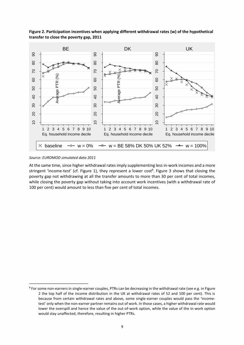
We begin by showing in Figure 2 the impact on participation incentives of using different withdrawal
rates of the hypothetical transfer to close the poverty gap. We remind that earned income components
are withdrawn at a rate of less than 100 per cent from the basic entitlement set at the poverty line,
whereas non-earned components - e.g. unemployment benefits and social assistance - are fully
withdrawn. Thus, as the withdrawal rate increases, less households pass the ‘income-test’ (i.e. the
withdrawn part surpasses the basic entitlement) and the difference between the remaining in- and
out-of-work transfers becomes smaller, which increases PTRs (cf. equation 2). Withdrawal rates of 58,
50 and 52 per cent maintain current average PTRs for the first three income deciles in Belgium,
Denmark and the UK.
7 The caveat of this approximation is that it does not include different treatments to both types of incomes which
might provoke some misallocations in the hypothetical transfer. This can be caused by e.g. different tax schedules for each source of income or the fact that some benefits are fully or partially exempted from taxation.
9
Figure 2. Participation incentives when applying different withdrawal rates (w) of the hypothetical transfer to close the poverty gap, 2011
Source: EUROMOD simulated data 2011
At the same time, since higher withdrawal rates imply supplementing less in-work incomes and a more stringent ‘income-test’ (cf. Figure 1), they represent a lower cost8. Figure 3 shows that closing the poverty gap not withdrawing at all the transfer amounts to more than 30 per cent of total incomes, while closing the poverty gap without taking into account work incentives (with a withdrawal rate of 100 per cent) would amount to less than five per cent of total incomes.
8 For some non-earners in single-earner couples, PTRs can be decreasing in the withdrawal rate (see e.g. in Figure
2 the top half of the income distribution in the UK at withdrawal rates of 52 and 100 per cent). This is because from certain withdrawal rates and above, some single-earner couples would pass the ‘income-test’ only when the non-earner partner remains out of work. In those cases, a higher withdrawal rate would lower the overspill and hence the value of the out-of-work option, while the value of the in-work option would stay unaffected, therefore, resulting in higher PTRs.
10
20
30
40
50
60
70
80
90
Avera
ge
PT
R (
%)
1 2 3 4 5 6 7 8 9 10
Eq. household income decile
BE
10
20
30
40
50
60
70
80
90
Avera
ge
PT
R (
%)
1 2 3 4 5 6 7 8 9 10
Eq. household income decile
DK
10
20
30
40
50
60
70
80
90
Avera
ge
PT
R (
%)
1 2 3 4 5 6 7 8 9 10
Eq. household income decile
UK
baseline w = 0% w = BE 58% DK 50% UK 52% w = 100%

10
Figure 3. Trade-off between participation incentives and costs when applying different withdrawal rates of the hypothetical transfer to close the poverty gap, 2011
Source: SILC 2012 and EUROMOD simulated data 2011 Note: costs are estimated as a proportion of current total (non-equivalised) incomes
Now we present the exact cost and impact on incentives of lifting all incomes just up to the poverty
line compared to including the extra expenditure (‘leakage’) needed to maintain participation
incentives at the bottom of the income distribution. In Table 1 we show the estimates of the poverty
headcount rate, the cost of closing the poverty gap and average PTRs in the first three equivalised
household income deciles. The first column presents the current situation, i.e. before estimating the
cost of closing the poverty gap. The second column shows the ‘mechanical’ cost (in relation to total
net incomes) of only closing the gap up to the poverty line. This means not taking work incentives into
account which is equal to applying a withdrawal rate of 100 per cent. The third column includes the
‘leakage’ needed to maintain the average PTRs in the first three income deciles at their present level.
20
30
40
50
60
70
80
Avera
ge
PT
R in
fir
st
3 d
ecile
s (
%)
05
10
15
20
25
30
35
40
Cost
as %
of
tota
l in
co
mes
0 20 40 60 80 100
withdrawal rate (%)
BE
20
30
40
50
60
70
80
Avera
ge
PT
R in
fir
st
3 d
ecile
s (
%)
05
10
15
20
25
30
35
40
Cost
as %
of
tota
l in
co
mes
0 20 40 60 80 100
withdrawal rate (%)
DK
20
30
40
50
60
70
80
Avera
ge
PT
R in
fir
st
3 d
ecile
s (
%)
05
10
15
20
25
30
35
40
Cost
as %
of
tota
l in
co
mes
0 20 40 60 80 100
withdrawal rate (%)
UK
cost (left axis) incentives (right axis)

11
Table 1. The cost of closing the poverty gap and PTR (in %)
Country Indicator Current scenario Closing poverty gap
with w = 100%
Closing poverty gap with w =
BE 58% DK 50% UK 52%
BE
Poverty 15.0
[14.0,16.0]
Cost 2.2 4.2
[1.9,2.5] [3.8,4.6]
Bottom PTRs
70.2 76.9 70.3
[69.2,71.2] [76.1,77.8] [69.8,70.9]
DK
Poverty 12.9
[11.7,14.0]
Cost 3.2 7.1
[2.4,3.9] [6.2,8.0]
Bottom PTRs
66.9 76.1 67.0
[65.2,68.6] [74.7,77.5] [66.4,67.5]
UK
Poverty 15.4
[14.6,16.2]
Cost 2.5 5.7
[2.2,2.8] [5.4,6.1]
Bottom PTRs
58.9 71.7 59.0
[58.9,59.5] [71.1,72.3] [58.6,59.3]
Source: SILC and EUROMOD simulated data 2011 Note: bottom means average in the first three equivalised household income deciles; costs are estimated as a proportion of current total (non-equivalised) incomes; in squared brackets 90 per cent confidence intervals (CI); CI of poverty estimates take into account the sample design of SILC (Goedemé, 2011; Zardo Trindade & Goedemé, 2016), while for PTRs we only assume the household as primary sampling unit due to lack of sample design variables.
If we focus on the current situation in the first column of Table 1 and the cost of lifting incomes up to
the poverty threshold in the second column, we see that Denmark presents the lowest poverty
headcount but the highest cost9, which implies that poverty is less frequent but deep in this country.
However, if households composed solely by students are removed, the estimate of the cost of closing
the poverty gap in Denmark would be just one percentage point higher than in the UK. Belgium
presents a higher poverty headcount but the lowest estimate of the cost of closing the poverty gap,
while poverty estimates are slightly worse in the UK but these differences are not statistically
significant.
When we analyse participation incentives, we see that Belgium combines the lowest cost estimate of
closing ‘mechanically’ the poverty gap with the highest current PTRs. The UK presents a slightly higher
cost estimate combined with the lowest PTRs, while Denmark has the highest cost estimate but in-
between PTRs. It is interesting to mention that when calculating the in-work components of the
formula of PTRs, in the UK the high average ratio of net in-work incomes to gross wages is achieved
with the lowest effective taxation (i.e. balance between taxes and benefits) on low gross incomes.
9 Although the cost difference with the UK is only statistically significant at an 85 percent confidence level.

12
Effective taxation on low incomes in the UK actually does not affect the ratio between in-work incomes
and gross wages, compared to decreases of 15 and 27 per cent in Belgium and Denmark.
The ‘mechanical’ cost of closing the poverty gap displayed in column 2 of Table 1 does not take work
incentives into account. As aforementioned and indicated in the same column, in this case PTRs would
worsen. Since some households might work less or not at all after these changes, the estimates at a
withdrawal rate of 100 per cent are very likely an underestimation of the true cost of closing the
poverty gap. As a consequence, if we want to close the poverty gaps in the three countries while
maintaining existing average participation incentives at the bottom of the income distribution, we
need to allow an important ‘leakage’ above the poverty line to working households. Due to different
poverty gaps and participation incentives imposed by tax-benefit systems, these leakage costs vary
considerably between Belgium, Denmark and the UK. In the third column, the cost includes the leakage
needed to maintain the average PTRs in the first three income deciles at their present level. This is
achieved with the withdrawal rates presented in Figure 2 of 58 per cent in Belgium, 50 per cent in
Denmark and 52 per cent in the UK. In Belgium, closing the poverty gap while keeping average PTRs
unchanged at the bottom of the income distribution would come at lower budgetary cost (4.2 per cent
of total net incomes) compared to Denmark (7.1 per cent) and the UK (5.7 per cent)10. We remind that
the source of funding is left unspecified, so any effects of increased taxes or contributions needed to
finance the hypothetical transfer are not taken into account.
The cost would be the lowest in Belgium because currently this country presents the lowest cost of
lifting incomes up to the poverty line and a comparatively low wedge between the in- and out-of-work
incomes involved in the calculations of PTRs. As we close the poverty gap, the leakage needed to
maintain low PTRs for working families is consequently relatively low - and can be achieved with a
relatively high withdrawal rate. The opposite is the case for the UK, which has to maintain the largest
wedge. Denmark presents the highest cost due to the relatively large cost of lifting incomes up to the
poverty line and also because despite not having the largest wedge between in- and out-of-work
incomes, it would allow the largest leakage. The reason why Denmark allows more leakage than the
UK with an even slightly lower withdrawal rate is because the Scandinavian country would need to
allocate around twice as much resources to household with earnings below the poverty line. As
earnings are not fully withdrawn, having a higher density of earnings below the poverty threshold ends
up being more costly.
The effort required to close the poverty gap maintaining participation incentives thus depends
importantly on the current incentives in each country, which vary substantially. It is interesting to see
in Figure 3 that at each level of PTRs, the withdrawal rate needed implies a cost of closing the poverty
gap that is always the most costly in Denmark and the least in the UK. For example, achieving in all
countries average PTRs of 50 percent at the bottom of the incomes distribution (without taking
behavioural reactions into account), it requires withdrawal rates that imply costs of roughly 15, 20 and
10 per cent of total incomes in Belgium, Denmark and the UK. Similarly, in Figure 4 we look at the costs
of closing the poverty gap in each country achieving its own and other countries’ average PTRs at the
bottom of the income distribution. For instance, the required withdrawal rate for the UK to close the
10 As a percentage of GDP, amounts are around half: 1.8 in Belgium, 3.3 in Denmark and 2.9 in the UK. As a
reference, social expenditure on cash benefits as a percentage of GDP in the branches of family (allowances and other), unemployment (compensation and severance pay) and other social policy areas (income maintenance and other) was 5.2 percent in Belgium and 2.9 per cent in Denmark and the UK (OECD, 2014b).

13
poverty gap without changing the average PTR of 59 per cent in the bottom deciles is 52 per cent. For
Belgium and Denmark reaching the PTRs of the UK would be achieved at a withdrawal rate of 37 per
cent, and therefore would be associated with substantially higher costs. The reason is that for reaching
this average PTR, substantially more resources should flow to working (poor and non-poor) households
in Belgium and Denmark as compared to current systems. In other words, the UK is already making a
‘gross-to-net’ effort that the other countries would need to make if they wanted to achieve stronger
participation incentives. Defining what are appropriate incentives in each country is beyond the scope
of this paper. However, the large differences suggest that in some countries, the magnitude of work
incentives might be reconsidered.
Figure 4. The cost of closing the poverty gap to achieve other countries’ average PTRs at the bottom of the income distribution
Source: SILC 2012 Note: Costs are estimated as a proportion of current total (non-equivalised) incomes. Country labels on top of x axis indicate current PTRs in the respective country.
Lastly, notice that keeping incentives at the extensive margin at the same level does not imply that
those at the intensive margin will also remain constant: as earned income is withdrawn from the
hypothetical transfer for working households, this is bound to increase EMTRs. To measure these
incentives, EMTRs follow the same logic of PTRs but instead of a change in wages from not working to
working, we use a marginal change in hours equal to five per cent, i.e. they represent how much of a
person’s gross income is taxed away when she works more hours11. That being said, the effect of
closing the poverty gap is rather different across countries due to important differences in current
EMTRs. Average EMTRs in the lowest three income deciles are 45 per cent in Belgium, 40 per cent in
Denmark and 63 per cent in the UK. Closing the poverty gap while allowing leakage to maintain average
PTRs in the lowest three deciles of the income distribution would increase EMTRs to 68 per cent in
11 Relevant assumptions of PTRs for people in work apply to EMTRs. The formula of EMTRs is 1 −
𝑦+5%−𝑦
𝑔+5%−𝑔.

14
Belgium, to 67 per cent in Denmark and just to 70 per cent in the UK. In this way, the results at both
the intensive and the extensive margin reflect the nature of current tax-benefit systems and the
interaction with the hypothetical transfer to close the poverty gap while allowing leakage. The UK
system already follows the general logic of the transfer, meaning that in this country they already
impose low PTRs and high EMTRs at the bottom of the income distribution. If Belgium and Denmark
would want to increase work incentives at the extensive margin in the same way, this would come at
the cost of worsening incentives to work more hours (higher EMTRs). Interestingly, among empirical
studies there is a growing agreement that labour force participation is more responsive to taxes and
transfers than hours worked12, especially at the bottom of the income distribution (Bargain et al., 2014;
Eissa, Kleven, & Kreiner, 2008; Immervoll et al., 2007). Therefore, it is relevant to bear in mind these
different behavioural responses when thinking about potential trade-offs between incentives at the
each margin.
5 Conclusion
If adequate social protection is to be taken seriously, it is important to offer adequate minimum
incomes and wages in combination with well-designed work incentives. All this would require
substantial additional welfare state effort. We found that the cost of closing the poverty gap without
worsening average participation incentives at the bottom of the income distribution would be around
two times the cost of just lifting all incomes to the level of the poverty threshold. This shows that a
balance between activation and protection would not be cheap and that some leakage would be
necessary. If instead of maintaining financial work incentives we would want to increase them, the
cost would be considerably higher in countries with comparably lower incentives such as Belgium and
Denmark. These countries would need to make ‘gross-to-net’ efforts for low income households that
the UK is already partially doing.
On a broader level, our results also illustrate the complexity of countries’ attempts to simultaneously
achieve each element of a ‘social trilemma’ – including reductions in poverty, expansions in
employment, with decreased (or at least non-increasing) social spending. Although our analysis is static
and we acknowledge that social investment might bring a reduction in social expenditures in the
future, our results can be seen as a first minimum estimate of the cost of a strategy balancing social
protection and financial work incentives (Vandenbroucke & Vleminckx, 2011). These findings point to
the fact that anti-poverty strategies also have to look at the drivers of rising market income inequality,
downward pressures on low wages and the issue of adequate work incentives.
12 Labour supply elasticities in Bargain et al. (2014) are calculated as the responses in hours to a one percent
increase in wages. As a reference, in 1998 in the countries we study, gross wage elasticities in the first quintile at the extensive margin were on average 0.36 and 0.15 for single and married people respectively, while just 0.02 at the intensive margin for both groups (the authors did not include the brake down of net wage elasticities).

15
References
Adam, S., & Browne, J. (2010). Redistribution, work incentives and thirty years of UK tax and benefit reform. IFS Working Paper, 70. Retrieved from http://citeseerx.ist.psu.edu/viewdoc/download?doi=10.1.1.974.9944&rep=rep1&type=pdf
Atkinson, A. B. (2010). Poverty and the EU: the New Decade. Macerata Lectures on European Economic Policy, Universita degli Studi di Macerata, May, 29. Retrieved from https://core.ac.uk/download/pdf/6565535.pdf
Bargain, O., Orsini, K., & Peichl, A. (2014). Comparing Labor Supply Elasticities in Europe and the United States New Results. Journal of Human Resources, 49(3), 723-838.
Bartels, C., & Pestel, N. (2015). The impact of short-and long-term participation tax rates on labor supply.
Cantillon, B., Collado, D., & Van Mechelen, N. (2015). The end of decent social protection for the poor? The dynamics of low wages, minimum income packages and median household incomes. Retrieved from
Cantillon, B., Van Mechelen, N., Pintelon, O., & Van den Heede, A. (2014). Social redistribution, poverty and the adequacy of social protection. In B. Cantillon & F. Vandenbroucke (Eds.), Reconciling Work and Poverty Reduction. How successful are European welfare states (pp. 157-184). New York: Oxford University Press.
Cantillon, B., & Vandenbroucke, F. (2014). Reconciling Work and Poverty Reduction: How Successful are European Welfare States? New York: Oxford University Press.
Corluy, V., & Vandenbroucke, F. (2014). Individual Employment, Household Employment, and Risk of Poverty in the European Union. A Decomposition Analysis. In B. Cantillon & F. Vandenbroucke (Eds.), Reconciling work and poverty reduction: how successful are European welfare states? (pp. 94-130). New York: Oxford University Press.
Decoster, A., Perelman, S., Vandelannoote, D., Vanheukelom, T., & Verbist, G. (2015). A bird’s eye view on 20 years of tax-benefit reforms in Belgium. CSB Working Paper, 45. Retrieved from http://www.centreforsocialpolicy.eu/sites/default/files/CSB%20Working%20Paper%2015%2002_April%202015.pdf
Eissa, N., Kleven, H. J., & Kreiner, C. T. (2008). Evaluation of four tax reforms in the United States: Labor supply and welfare effects for single mothers. Journal of Public Economics, 92(3–4), 795-816. doi:http://dx.doi.org/10.1016/j.jpubeco.2007.08.005
European Commission. (2013). Communication from the Commission to the European Parliament and the Council. Strengthening of the Economic and Monetary Union. (COM(2013) 690 final). Brussels: European Commission.
Eurostat. (2015). Complete database. Retrieved from http://ec.europa.eu/eurostat/data/database Figari, F., Paulus, A., & Sutherland, H. (2015). Chapter 24 - Microsimulation and Policy Analysis. In B.
A. Anthony & B. François (Eds.), Handbook of Income Distribution (Vol. Volume 2, pp. 2141-2221): Elsevier.
Goedemé, T. (2011). How much Confidence can we have in EU-SILC? Complex Sample Designs and the Standard Error of the Europe 2020 Poverty Indicators. Social Indicators Research, 110(1), 89-110. doi:10.1007/s11205-011-9918-2
Hacker, J. (2011). The institutional foundations of middle-class democracy. Policy Network. Retrieved from Policy Network website: http://www.policy-network.net/pno_detail.aspx?ID=3998&title=The+institutional+foundations+of+middle-class+democracy
Hemerijck, A. (2012). Changing welfare states: Oxford University Press. Immervoll, H. (2007). Minimum Wages, Minimum Labour Costs and the Tax Treatment of Low-Wage
Employment. Discussion Paper Series. Retrieved from http://www.oecd-

16
ilibrary.org/docserver/download/5l4w2bvsd0nt.pdf?expires=1458304235&id=id&accname=guest&checksum=A997DBA27DC139904123EF5B9FAD7315
Immervoll, H., Kleven, H. J., Kreiner, C. T., & Saez, E. (2007). Welfare reform in European countries: a microsimulation analysis. The Economic Journal, 117(516), 1-44.
Iversen, T., & Wren, A. (1998). Equality, employment, and budgetary restraint: the trilemma of the service economy. World politics, 50(04), 507-546.
Kampelmann, S., Garnero, A., & Rycx, F. (2013). Minimum wages in Europe: does the diversity of systems lead to a diversity of outcomes? (128). Retrieved from Brussels:
Marchal, S., & Marx, I. (2015). Stemming the Tide: What Have EU Countries Done to Support Low-Wage Workers in an Era of Downward Wage Pressures? IZA Discussion Papers. Retrieved from http://ftp.iza.org/dp9390.pdf
Marx, I., Marchal, S., & Nolan, B. (2013). Mind the Gap: Net Incomes of Minimum Wage Workers in the EU and the US. In I. Marx & K. Nelson (Eds.), Minimum Income Protection in Flux (pp. 54-80): Palgrave Macmillan.
OECD. (2005). OECD Employment Outlook 2005. Retrieved from Paris: /content/book/empl_outlook-2005-en
http://dx.doi.org/10.1787/empl_outlook-2005-en OECD. (2009). OECD Employment Outlook 2009. Retrieved from Paris: /content/book/empl_outlook-
2009-en
http://dx.doi.org/10.1787/empl_outlook-2009-en OECD. (2014a). In It Together: Why Less Inequality Benefits All. Retrieved from Paris:
/content/book/9789264235120-en
http://dx.doi.org/10.1787/9789264235120-en OECD. (2014b). OECD.Stat (database) (Publication no. http://dx.doi.org/10.1787/data-00285-en). Sutherland, H., & Figari, F. (2013). EUROMOD: the European Union tax-benefit microsimulation
model. Retrieved from Van Lancker, A. (2010). Working document on a Framework Directive on Minimum Income.
Retrieved from http://europeanemployers.com/doc/EAPN_draft_directive_on_mimimum_wage,_Sep_2010.pdf
Van Mechelen, N., & Marchal, S. (2012). Struggle for life: social assistance benefits, 1992-2009. In I. Marx & K. Nelson (Eds.), Minimum income protection in flux (pp. 28-53). Great Britain: Palgrave Macmillan.
Van Mechelen, N., & Marchal, S. (2013). Trends and convergence of Europe’s minimum income schemes. ImPRovE working paper, 13/11. Retrieved from http://improve-research.eu/?wpdmact=process&did=MjkuaG90bGluaw==
Vandenbroucke, F., Cantillon, B., Van Mechelen, N., Goedemé, T., & Van lancker, A. (2013). The EU and Minimum Income Protection: Clarifying the Policy Conundrum. In I. Marx & K. Nelson (Eds.), Minimum Income Protection in Flux (pp. 271-317). Hampshire: Palgrave Macmillan.
Vandenbroucke, F., & Vleminckx, K. (2011). Disappointing poverty trends: is the social investment state to blame? Journal of European Social Policy, 21(5), 450-471. doi:10.1177/0958928711418857
Zardo Trindade, L., & Goedemé, T. (2016). Notes on updating the EU-SILC UDB sample design variables, 2012 and 2013. CSB Working Paper. Retrieved from http://www.centrumvoorsociaalbeleid.be/index.php?q=publicaties/workingpapers/en

17
Appendix
Appendix A – Participation tax rates
Similar methods to calculate PTRs can be found in Adam and Browne (2010) and Decoster, Perelman,
Vandelannoote, Vanheukelom, and Verbist (2015). As in the application of the latter, we do not
differentiate between individuals working different numbers of hours. To build the Heckman selection
model we need variables that are not included in the EUROMOD input file; therefore, we merge these
files with SILC and FRS. It is relevant to mention that EUROMOD input files are not based on version 3
of SILC 2012 but on the Belgian version and on version 1 in Denmark. The resulting files using SILC
present some inconsistencies to calculate hourly wages. First, the declared number of months working
and gross wage from employment are not always coherent. Second, some people respond to be
working both part- and full-time and the weekly amount of hours worked corresponds only to the main
job. Third, some respondents declare to work for too many or too few hours, so we assume that
working between 30 and 70 hours for full-time workers and less than 36 for part-time workers are
realistic amounts. To deal with all these situations, in the model we only use the hourly wages from
people with consistent information and we impute the wages of people without consistent data. In
the UK we get from FRS the gross wage of employed people in their first job to use in the model and
we make the same assumptions about realistic amounts of hours. The variables that we use for the
wage equation in the Heckman model are education, age and experience (including squared terms),
migration status, and for women region. The extra variables necessary for the selection equation are
region for men and for women the presence of children younger than three years old, between four
and six, between seven and 12 and between 12 and 18 (in Denmark we use the children variables for
both genders as there is no region variable). With this information we predict log hourly wages
separately for men and women. We bottom code hourly wages so they are not below legal minima. In
Belgium we used six euros (following Decoster et al., 2015), in the UK six pounds (OECD, 2014b) and in
Denmark 102 Danish Crones (lowest collective agreement in Kampelmann, Garnero, & Rycx, 2013
corrected by EUROMOD wages inflation index). We define as available for work people between 20
and 64 who are employed or self-employed. We do not calculate the PTR of households and individuals
receiving non-simulated benefits because they cannot be adapted to changes in wages. In contrast, we
do calculate PTR of workers whose partners are receiving non-simulated individual benefits as we
believe that the benefits involved would not change much when partner’s wages are modified. In
Belgium and Denmark, if the partner of the person whose PTR is being calculated receives an
unemployment benefit, we also simulate it using the predicted hourly wage recalculated to a full-time
full-year basis. Self-employed people presents wages that are often below the aforementioned legal
minima. Therefore, with the same wage equation of the Heckman model but using a simple regression,
we impute in the same way self-employed hourly wages. We do the same for employed people without
consistent data.

18
Table 2. Heckman selection model results
BE DK UK
Men Women Men Women Men Women
Coef. p-value Coef. p-value Coef. p-value Coef. p-value Coef. p-value Coef. p-value
log hourly wage equation
ISCED Education level 4 0.078 0.099 0.045 0.316 Omitted Omitted 0.375 0.000 0.198 0.000
ISCED Education level 5 0.324 0.000 0.343 0.000 0.169 0.000 0.131 0.006 0.659 0.000 0.488 0.000
age 0.018 0.340 0.009 0.462 0.030 0.207 0.041 0.051 0.072 0.000 0.026 0.000
age squared 0.000 0.377 0.000 0.432 0.000 0.427 0.000 0.235 -0.001 0.000 0.000 0.000
(years of)experience 0.002 0.004 0.002 0.000 0.001 0.508 0.000 0.667 0.004 0.000 0.002 0.000
experience squared 0.000 0.189 0.000 0.010 0.000 0.041 0.000 0.132 0.000 0.103 0.000 0.000
immigrant 1 -0.105 0.029 -0.061 0.107 0.037 0.692 0.213 0.080 0.144 0.000 0.063 0.012
immigrant 2 -0.011 0.882 -0.050 0.453
region 2 -0.083 0.004 -0.066 0.012
region 3 -0.078 0.015 -0.001 0.940
region 4 -0.072 0.001
constant 2.152 0.000 2.254 0.000 4.364 0.000 4.004 0.000 0.470 0.011 1.468 0.000
employment equation
ISCED Education level 4 0.271 0.261 0.283 0.312 Omitted Omitted 0.370 0.099 0.205 0.035
ISCED Education level 5 0.807 0.000 0.447 0.000 0.588 0.032 0.222 0.268 0.777 0.063 0.545 0.000
age 0.031 0.599 -0.028 0.393 -0.255 0.044 0.047 0.640 0.133 0.020 -0.066 0.000
age squared -0.002 0.004 -0.001 0.017 0.003 0.038 0.000 0.679 -0.003 0.000 0.000 0.739
(years of)experience 0.012 0.000 0.015 0.000 0.010 0.088 0.001 0.816 0.005 0.001 0.012 0.000
experience squared 0.000 0.448 0.000 0.000 0.000 0.054 0.000 0.497 0.000 0.000 0.000 0.000
immigrant 1 -0.320 0.089 -0.488 0.000 -0.357 0.324 0.269 0.546 -0.027 0.063 0.090 0.078
immigrant 2 0.532 0.115 -0.240 0.444
region 2 0.555 0.001 -0.001 0.991 0.137 0.062 0.107 0.215
region 3 0.213 0.206 -0.089 0.467 -0.020 0.041 0.055 0.235

19
region 4 -0.054 0.043 -0.004 0.946
children below 3 -0.346 0.000 0.819 0.020 0.081 0.591 -0.593 0.000
children between 3 and 6 -0.269 0.003 -0.022 0.905 0.199 0.219 -0.386 0.000
children between 6 and 12 -0.042 0.579 0.551 0.002 0.208 0.128 -0.227 0.000
constant 0.389 0.727 1.591 0.014 4.991 0.013 -0.021 0.991 -1.790 0.000 1.589 0.000
correlation between the error terms of equations (rho)
-0.032 0.711 0.043 0.636 -0.234 0.000 0.907 0.000 0.920 0.000 -0.110 0.050
number of observation total in work total in work total in work total in work total in work total in work
1758 1496 2166 1496 1811 1754 1759 1658 7150 5428 8344 5608 Note: 95 per cent confidence level; reference categories are ISCED Education level 0-3, non-immigrant, region 1, children between 12 and 18; in Belgium immigrant 1
corresponds to non-EU, in Denmark to EU and immigrant 2 to non-EU and in the UK immigrant 1 to non-British; in Belgium region 1 is Brussels, 2 Flanders and 3 Wallonia, in
the UK region 1 is England, 2 Wales, 3 Scotland and 4 Northern Ireland; omitted variables due to collinearity; results of the regression to impute the hourly wages of self-
employed and employed people without consistent data are not included because they are rather similar.
Source: SILC and FRS 2012

Appendix B – Income components
Table 3. Income components of net non-earned and earned incomes in EUROMOD datasets
BE FI UK
Non-earned Earned Non-earned Earned Non-earned Earned
Net Net Net
+ Gross + Gross + Gross + Gross + Gross + Gross
- proportional income & municipal tax and maintenance payments
- proportional income tax, municipal tax and maintenance payments
- proportional taxes and maintenance payments
- proportional taxes and maintenance payments
- proportional income tax and maintenance payments
- proportional income tax and maintenance payments
- Investment & property tax, pension & disability contributions
- Employee, special & self-employed contributions
- Capital & property tax
- Employee & self-employed contributions
- Council Tax - Employee & self-employed contributions
+ Work bonus + Working tax credit
Gross Gross Gross
+ investment income
+ income from employment and self-employment
+ investment income
+ income from employment and self-employment
+ investment income
+ income from employment and self-employment
+ income of children under 16
+ income of children under 16
+ income of children under 16
+ property income
+ property income
+ property income
+ private pension
+ private pension
+ personal pension
+ received transfers
+ received transfers
+ received transfers
+ benefits + benefits + benefits
+ income from odd jobs
Table 4. Income components of net non-earned income and net earned income in SILC datasets
Non-earned Earned
Net
+ Gross + Gross
- proportional tax on income and social insurance contributions and maintenance payments (HY140G+HY130G)
- proportional tax on income and social insurance contributions and maintenance payments (HY140G+HY130G)
- Investment & property tax (HY120G)
Gross
+ investment income (HY090G) + income from employment and self-employment (PY010G+PY050G)
+ income of children under 16 (HY110G)
+ property income (HY040G)
+ private pension (PY080G)
+ received transfers (HY080G)
+ Benefits (PYG:90+100+110+120+130+140+ HYG: 50+60+70)
Note: in parenthesis the name of the variables in SILC.
Top Related