


Languages
Pages
Legal


WORKING PAPER SERIES
The Effectiveness of Monetary Policy
Robert H. Rasche and
Marcela M. Williams
Working Paper 2005-048B http://research.stlouisfed.org/wp/2005/2005-048.pdf
June 2005 Revised July 2005
FEDERAL RESERVE BANK OF ST. LOUIS Research Division 411 Locust Street
St. Louis, MO 63102 ______________________________________________________________________________________
The views expressed are those of the individual authors and do not necessarily reflect official positions of the Federal Reserve Bank of St. Louis, the Federal Reserve System, or the Board of Governors.
Federal Reserve Bank of St. Louis Working Papers are preliminary materials circulated to stimulate discussion and critical comment. References in publications to Federal Reserve Bank of St. Louis Working Papers (other than an acknowledgment that the writer has had access to unpublished material) should be cleared with the author or authors.
Photo courtesy of The Gateway Arch, St. Louis, MO. www.gatewayarch.com

The Effectiveness of Monetary Policy
Robert H. Rasche Marcela M. Williams
July, 2005
Abstract: The analysis addresses changing views of the role and effectiveness of monetary policy, inflation targeting as an “effective monetary policy,” monetary policy and short-run (output) stabilization, and problems in implementing a short-run stabilization policy. JEL Codes: E520 Keywords: monetary policy, inflation targeting, short-run stabilization policy
1

The Effectiveness of Monetary Policy
Robert H. Rasche Marcela M. Williams
Federal Reserve Bank of St. Louis*
Introduction
The question of the effectiveness of monetary policy is a long-standing issue in
the literature of monetary economics and central banking. Perspectives on the question
have been influenced, in part, by developments in monetary theory, in part by
interpretations of monetary history. Progress in the discussion has also been influenced,
indeed some might say hindered, by changing definitions of both “monetary policy” and
“effectiveness.” Our discussion will address 1) changing views of the role and
effectiveness of monetary policy, 2) inflation targeting as an “effective monetary policy,”
3) monetary policy and short-run (output) stabilization, and 4) problems in implementing
a short-run stabilization policy.
1. Changing Views on the Role and Effectiveness of Monetary Policy.
What do analysts mean by “monetary policy” and the “effectiveness” thereof?
Both terms are something of moving targets. At times “monetary policy” has referred to
central bank actions to influence and/or target some measure of the money stock.
Frequently, though certainly not always, the definition of monetary policy focused on a
measure of “high powered money” – liabilities of the central bank. For a long time, this
was the definition incorporated in theoretical models. In the policy arena this
* The authors are Senior Vice President and Director of Research and Senior Research Associate, respectively. The views expressed are the authors’ and do not necessarily reflect official positions of the Federal Reserve System.
2

definition was the foundation of the “monetarist revolution” in the 1960s and 70s. A
counter definition that was likely the dominant perspective of policymakers was that
monetary policy referred to central bank actions to influence and/or target short-term
interest rates or nominal exchange rates. Sargent and Wallace (1975) advanced the
proposition that, in a model with “rational expectations,” the price level (and all other
nominal variables) could be indeterminate if central banks set targets for nominal interest
rates, because the economy would lack a “nominal anchor.” McCallum (1981) showed
that an appropriately defined interest rate rule would avoid such indeterminacy. The
interest rate rule had to include a “nominal anchor.” In recent years, in particular since
Taylor’s (1993) proposed characterization of FOMC behavior in the early Greenspan
years, interest rate rules that include a “nominal anchor” in the form of a desired or target
inflation rate, have become the basic specification of “monetary policy” in theoretical
analyses [see for example, Clarida, Galí, and Gertler (1999)].
The legacy of the Great Depression in the United States and other industrialized
economies was that monetary policy was “ineffective.” This perspective is most
prominent in Keynes’ General Theory and in the writings of the “Keynesian economists”
in the 1940s through the 1960s. For example, the Radcliffe Committee in the United
Kingdom reported:
The immediate object of monetary policy action is to affect the level of total demand. … In theory, monetary action may work upon total demand by changing the interest incentive; we believe that only very limited reliance can be placed on this. More certainly, monetary action works upon total demand by altering the liquidity position of financial institutions and of firms and people desiring to spend on real resources; the supply of money itself is not the critical factor.1
1 Committee on the Workings of the Monetary System: Report, p. 135
3

In the United States the minimalist perspective on the role and effectiveness of monetary
policy can be seen in the first two Reports of the Kennedy Council of Economic
Advisers:
Unless the Government acts to make compensating changes in the monetary base, expansion of general economic activity, accompanied by increased demands for liquid balances and for investment funds will tend to tighten interest rates and restrict the availability of credit. … Discretionary policy is essential, sometimes to reinforce, sometimes to mitigate or overcome, the monetary consequences of short-run fluctuations of economic activity. In addition, discretionary policy must provide the base for expanding liquidity and credit in line with the growing potential of the economy.2
and:
Monetary policy as well as debt management policy must be coordinated with fiscal policy to secure the objectives of high employment and growth without inflation. We are, and for some time still will be, in a situation of substantial slack in labor force and capital resources, a situation in which expansionary policies are required. … What matters most at this time is that financial policy should be designed to facilitate rather than retard the expansionary process which the tax program is designed to launch.3
A decade later, perspectives on the effectiveness of monetary policy had changed;
and, in some circles, monetary policy was viewed as equally important as fiscal policy for
affecting both inflation and output fluctuations:
The past 10 years have been characterized by an average growth rate of aggregate expenditures that is very high by historical standards and that has substantially outstripped the sustainable growth of supply of real goods and services. Contributing significantly to the growth of aggregate demand were rapidly increasing Government expenditures along with monetary policies that were appreciably more expansionary than those in earlier post-World War II periods. … When the inflationary phase has lasted so long that expectations of further inflation are firmly embedded in the cost trend, a shift to policies of restraint first exerts an adverse influence on output and the desired price
2 Economic Report of the President, Jan 1962, p. 85. 3 Economic Report of the President, Jan 1963, p. 55.
4

deceleration effect materializes only with a lag. Any convincing interpretation of the events during 1970 and 1973-4 must stress this difficulty.4
This was not the only view of monetary and fiscal policy at that time. The 1960s
saw the rise of “monetarism” subsequent to the work of Friedman and Schwartz (1963),
Friedman and Meiselman (1963), and Andersen and Jordan (1968). There were several
planks in the monetarism platform. First and foremost was that sustained inflation was a
monetary phenomenon and that central banks should be held accountable for maintaining
price stability. Monetarists contended that central banks should control the stock of
money in the economy, and not focus on targeting short-term nominal interest rates, as
the mechanism to achieve this long-run inflation objective. The rationale for the focus on
the growth of the money stock was that, in a fiat money economy, the money stock
provided the nominal anchor for the system.
In the eyes of monetarists, inflation control was not the only concern of the
monetary authorities. They saw monetary policy as having significant effects on short-
run fluctuations in real output (Andersen and Jordan, 1968; Andersen and Carlson,
1970), though not affecting long-run output growth. Indeed many monetarists (see
Brunner and Meltzer, 1968; Meltzer, 1995, 2003; and Friedman and Schwartz, 1963) saw
monetary policy as responsible for aggravating, not attenuating historical cyclical
fluctuations in real output.
With the “rational expectations revolution” in macroeconomics came the “policy
ineffectiveness proposition” of the New Classical Macroeconomics (Sargent and
Wallace, 1975). The initial interpretations of this paradigm were that, in any
macroeconomic model, the assumption of rational expectations would render monetary
4 Economic Report of the President, February, 1975, pp. 128-9
5

policy ineffective in influencing real output, both in the short run and long run. Hence
there was no role for monetary policy in output stabilization. Subsequent research
(Fischer, 1977, Taylor, 1980, and Calvo, 1983) demonstrated that it was the interaction of
the rational expectations hypothesis and an assumption of perfectly flexible wages and/or
prices that generated the “policy ineffectiveness proposition.” The outgrowth of this
insight was the “New Keynesian” perspective.
With the widespread use of “New Keynesian” models, the monetarist tenets about
how “monetary policy” impacts economic activity are widely held throughout academia
and central banking circles today, though most academics and almost all central bankers
would disown a monetarist label. Money has largely disappeared from discussions on
monetary policy. Fry et al. (2000), utilizing data from a Bank of England survey, report
that in the 1970s 11 (of 22) central banks in industrial countries reported using a money
and credit framework to formulate monetary policy; but, that by the 1990s, only 2 of
these banks maintained this framework.5 Von Hagen (2004) found a negative trend from
1970 – 2002 in the fraction of titles of articles in major economics journals that included
the word “money,” though the frequency of titles including “inflation” was relatively
constant.6 He also found that the frequency of “money” in the annual reports of major
central banks declined over the period 1996-2002.7 King (2002) notes:
… there is a paradox in the role of money in economic policy. It is this: that as price stability has become recognized as the central objective of central banks, the attention actually paid by central banks to money has declined.8
5 Fry et al., (2000), Chart 7.2, p. 123. 6 Von Hagen (2004), Table 4. 7 Von Hagen, (2004), Table 5 8 King, (2002), p. 162
6

The decline and fall of money in policy formation is confirmed by a fall in the number of references to money in speeches of central bank governors. So much so that over the past two years, Governor Eddie George has made one reference to money in 29 speeches, Chairman Greenspan one in 17, Governor Hayami one in 11 and Wim Duisenberg three in 30.9
In contemporary literature, models, and policy discussions, attention is given to
the role of an inflation objective in a central bank “policy rule” as the nominal anchor in a
fiat money economy. “Taylor rules” (Taylor, 1993) that specify a systematic relation
between the target for a short-term interest rate and deviations of inflation from an
inflation target and real output from a measure of “potential output” have become the
norm for the analysis of the impact of monetary policy.10 In this “rule like” environment,
the setting of the interest rate value is the policy action; the policy itself is represented by
the parameters of the “rule,” including the inflation objective ( ) and the respective
weights that are assigned to deviation of observed inflation from that objective and
deviations of real output from “potential output.”
*π
2. Long-run Stabilization Objectives for Monetary Policy
Over the past 15 years, a number of countries, starting with New Zealand, have
announced explicit numeric inflation objectives (the term in the Taylor rule
framework.) The relevant question is how effective are central banks at hitting explicit
numeric inflation targets?
*π
Clearly one straightforward way to address the question of the effectiveness of
monetary policy is to look at the performance of those countries that have announced
9 King, (2002), p. 162-3. 10 There is an active discussion in the contemporary literature over the design of monetary policy rules. Some economists (for example, Svensson, 2005) argue for instrument rules that are optimized from an objective function of the central bank and models of the macroeconomy. Others (for example, McCallum and Nelson, 2004) argue for independently constructed target rules in the spirit of Taylor (1993). Both sides in this debate appear to accept the proposition that monetary policy can impact both inflation and real
7

explicit numeric inflation targets. Our list of the countries in this group is shown in Table
1. We have identified a total of 21 countries that continue to pursue such targets.11 The
initial inflation under which the target was adopted by each of these countries is graphed
against the year of adoption in Figure 1.12 As far as we have been able to determine, no
country has joined the group since 2002. In many, but certainly not all of these countries,
inflation was below 5 percent at the time of the announcement of the inflation targeting
regime. Table 2 provides the details on the target index(es), the target ranges, dates of
adoption for the target, responsibility for target setting, and public reporting on the
performance of the inflation policy.
Figures 2-22 show the history of inflation for each of the inflation targeting
countries.13 There are multiple graphs for those countries that have changed the index in
which they define their inflation target – one graph for each index used. The graphs
show the inflation target range (the shaded area) or the point inflation target as
appropriate. It is immediately apparent from these graphs that the period-to-period
(month-to-month or quarter-to-quarter) annualized rate of inflation is highly volatile in all
of the countries that pursue an explicit numeric inflation target. These short-run inflation
rates are as likely as not to be outside of the target range. If effective monetary policy
were to be defined in terms of stability of high-frequency rates of inflation, then all of
these central banks would have to be judged as failing to achieve the objective.
However, it is neither reasonable nor desirable to define the objective in such short-run
output in the short run, but only inflation in the long run. Hence this theoretical debate is about how to best implement monetary policy rules, not about the effectiveness of policy. 11 We consider three countries that at one time had explicit numeric targets − Finland, Spain, and Greece − that have dropped from the group upon accession to the EMU. 12 This graph updates similar graphs that can be found in Loayza and Soto (2002) and Mishkin and Schmidt-Hebbel (2002).
8
terms. Shocks to the price level − that is transitory shocks to inflation − originate from
numerous sources, both monetary and nonmonetary. No central bank can foresee such
shocks and probably cannot accurately predict the dynamics by which such shocks
ultimately impact the price level. Economic theory suggests that central banks can be
held accountable for “sustained inflation.” Correspondingly, inflation targeting central
banks, and even central banks without explicit numeric targets such as the Fed, typically
focus on “medium term” inflation. The duration of the “medium term,” frequently, and
probably intentionally, is left ambiguous.14 Absent a precise definition of the “medium
term” some measures must be specified to judge the “effectiveness” of the inflation
targeting policies.
We examine two measures of the effectiveness of explicit numeric inflation
targeting. Both measures are based on moving averages of the observed rates of
inflation. These measures are indicated by the red (heavy) line in the figures. Relative to
the dates indicated on the horizontal axis, this line shows the leading moving average rate
of inflation to the end of 2004. The shortest moving average shown is one year. The
question is what is the maximum period, ending with 2004, that the moving average of
the inflation rate remained within the bounds determined by the current (end of 2004)
inflation target? These periods are shown for each of the inflation targeting countries in
Table 3.
Judged by this metric, there are a number of inflation targeting countries in which
monetary policy has been very effective. For five countries, New Zealand, Norway,
13 For early discussions of the implementation and experience of several of these countries with inflation targeting, see Leiderman and Svensson (1995).
9

Switzerland, Thailand, and the United Kingdom the moving average rate of inflation has
been within the current announced target range since before the adoption of the inflation
targeting procedure.15 Canada and Australia also have maintained average inflation
within the range currently in effect for considerable periods (note that for Australia and
New Zealand, data are quarterly, not monthly.) None of these countries has a particularly
wide target range. The Czech Republic and South Africa have shorter records of success
by this metric but, nevertheless moderately, effective performances. The Czech Republic
is notable, since the inflation rate there was fairly high when the target was adopted, and
the moving average inflation has fallen outside of the target range only on the low side.
Nevertheless, the moving average of Czech headline inflation has been positive for the
entire period since it fell below the lower bound of the current target range (in February
2002.) Israel, Peru, and Poland have experienced long-term average inflation below
their current target ranges. The short-horizon moving averages for Hungary, Peru, and
Poland have exceeded the current target range. In Israel the moving average inflation
rate actually went negative in 2002 and 2003. Three countries, Chile, Colombia, and
Hungary have adjusted their targets downward over time and generally the average
inflation rate has fallen below the ranges, consistent with success in moving to the lower
inflation targets. Failure to stay in the target ranges has not been asymmetric. Other
countries, notably Brazil, Mexico, and the Philippines have consistently missed their
target ranges on the high side.
14 President Santomero of the Federal Reserve Bank of Philadelphia has stated that he prefers measuring inflation against an explicit target range on a 12-month moving average (year-over-year) basis. Few central bankers have been this explicit about their definitions of a “medium term.” 15 Norway has a stated target of 2.5 percent, not an inflation range. The moving average inflation rate has been below this value since 2000 and only dipped slightly below zero in early 2003.
10
While averages provide interesting insights into the sustainability of the inflation
performance, they obscure the marginal performance. A moving average could remain
within the target range for a long period of time because, over time, the inflation rate is
converging towards the midpoint of the range. Alternatively, the same moving average
could result because, early in the period, the inflation rate was close to one end point of
the target range and, as time progressed, inflation moved close to the opposite edge of the
target range. The latter situation could be characterized as “skating on thin ice.”
To examine this issue, Table 3 shows the value of the moving average over the
two-year period 2003-4 and a standardized deviation of this two-year moving average
from the midpoint of the target range that prevailed at the end of 2004. The
standardization is constructed by dividing the deviation of the moving average from the
midpoint by one-half the difference between the upper and lower endpoints of the target
range.
By this metric the bulk of the inflation targeting countries are doing quite well in
the past two years. The exceptions are Brazil, Colombia, Hungary, Mexico, and the
Philippines (whose average inflation rate over the past two years fell above their target
ranges) and Israel and Sweden (whose average inflation rate over the past two years fell
below the target ranges.)
Our conclusion from these data is that, where countries have announced explicit
numeric inflation objectives for their central banks, central banks have been quite
effective in achieving the stated inflation stabilization objective.
The FOMC has not adopted this framework, though it is known that on at least
three occasions the pros and cons of adopting this approach have been debated around the
11

FOMC table.16 Several current participants in the FOMC have stated on the record their
preference for explicit numeric targets and given their preferred measures. Included are
Governor Ben Bernanke, President Jeffrey Lacker of the Richmond Fed, President Janet
Yellen of the San Francisco Fed, and President Anthony Santomero of the Philadelphia
Fed.17
Governor Bernanke has indicated his preferred inflation target is 1-2 percent as
measured by the core personal consumption price index.18 President Lacker indicated his
preference for a target of 2 percent as measured by the core CPI price index or 1.5 as
measured by the core personal consumption price index. He also indicated a preference
that inflation be kept above 1 percent.19 President Yellen has indicated a preference for a
target of 1.5 percent as measured by the core personal consumption price index, with a
range of about ± 1 percent.20 President Santomero has indicated his preference for a
target range of 1-3 percent as measured by a 12-month moving average rate of change in
the core personal consumption price index.21 Other current participants at FOMC
meetings, including Governor Donald Kohn (2005), have indicated that they do not prefer
an explicit numeric inflation objective. President William Poole has stated that he
16 Transcripts of two of these debates, on January 31, 1995 and July 2, 1996 can be found on the Web site of the Board of Governors:< http://www.federalreserve.gov/fomc/transcripts/transcripts_1995.htm>; <http://www.federalreserve.gov/fomc/transcripts/transcripts_1996.htm>. A summary of the most recent debate at the February 1, 2005, FOMC meeting is also available on the Board’s Web site <http://www.federalreserve.gov/fomc/minutes/20050202.htm>. 17 During the July 1996 FOMC debate on inflation targets, President Gary Stern of the Federal Reserve Bank of Minneapolis indicated that a 2 percent target (in terms of the CPI) would be acceptable to him. (FOMC Transcripts, July 2-3, 1996, p. 56) The discussion at that time was not framed in terms of a target point or a target range. 18 For instance B.S Bernanke remarks at Stanford University, February 11, 2005. Reported by Michael Derby Dow Jones Commodity Wire, February 11, 2005. 19 J.M. Lacker, “Inflation Targeting and the Conduct of Monetary Policy,” University of Richmond Robins School of Business, March 1, 2005. <http://www.rich.frb.org/media/speeches/index.cfm/id=70>. 20 “Fed’s Yellen says inflation target has some merit,” Reuters News, February 11, 2005. 21 “Santomero: Fed should adopt explicit inflation target,” AFX Asia, October 4, 2004.
12

believes “ambiguity with respect to the Fed’s inflation and employment objectives is not
large and is not the main problem the Fed faces with its communication policies.”22
Differences of opinion among FOMC participants notwithstanding, in May 2003
the press release following the FOMC meeting indicated that “the probability of an
unwelcome substantial fall in inflation, though minor, exceeds that of a pickup in
inflation from its already low level.”23 The minutes of that FOMC meeting indicate the
rationale for this statement:
Members commented that substantial additional disinflation would be unwelcome because of the likely negative effects on economic activity and the functioning of financial institutions and markets, and the increased difficulty of conducting an effective monetary policy, at least potentially in the event the economy was subjected to adverse shocks. Members also agreed that there was only a remote possibility that the process of disinflation would cumulate to the point of a decline for an extended period in the general price level.24
At that time, core personal consumption inflation was in the neighborhood of 1
percent. Since FOMC participants who have expressed preferences in terms of both the
core CPI and core personal consumption price index have typically indicated values for
core CPI inflation a half percent above those for the core personal consumption inflation
rate, it seems reasonable to conclude that the FOMC has a lower bound of an acceptable
medium-term rate of inflation in the neighborhood of 1 percent for the core personal
consumption inflation rate and perhaps 1.5 percent for the core CPI inflation rate.
Former Governor Larry Meyer (2001) is also on record in favor of an explicit
numeric inflation objective. However, his position is that the “dual mandate” inherent in
22 “How Should the Fed Communicate,” Princeton University, April 2, 2005. <http://stlouisfed.org/news/speeches/2005/4_02_05.htm>. 23 <http://federalreserve.gov/boarddocs/press/monetary/2003/20030506/default.htm>
13

the Federal Reserve Act differentiates the U.S. environment from that of other inflation
targeting central banks that operate under a “hierarchical mandate.” Meyer defines a
“hierarchical mandate” as an environment “where price stability is identified as the
principal objective, and central banks are restricted from pursuing other objectives unless
price stability has been achieved.”25 He contrasts this with the “dual mandate” where
“monetary policy is directed at promoting both full employment and price stability with
no priority expressed, and with the central bank responsible for balancing both these
objectives in the short run.”26
It is our opinion that Meyer’s view does not allow for the different in the
effectiveness of monetary policy in the long and short run. In terms of long-run
objectives, central banks must necessarily operate under a hierarchical mandate, given the
consensus view of monetary policy that policymakers are not presented a long-run
tradeoff between inflation and real output. Indeed, in specifying a policy rule, whether an
instrument or target rule, the exercise of determining how much weight to place on short-
run movements in inflation versus short-run movements in real output is conditioned on
the prespecification of the long-run inflation target ( ). In this sense any central bank
seeking to operate in such a monetary policy framework has to be hierarchical: first it
must specify its long-run inflation objective and then, and only then, can it set its
preferred (or optimal) weights for short-run fluctuations.
*π
27 The choice of weights could
be such that the central bank follows a hierarchical mandate in both the long and short
run; however there is nothing to preclude pursuing a dual short-run mandate nested
24 < http://www.federalreserve.gov/fomc/minutes/20030506.htm> 25 Meyer (2001), p. 151. 26 ibid.
14

within a hierarchical long-run mandate. It is likely that most, if not all, central banks that
have adopted an explicit inflation target pursue that objective within a nested
hierarchical/dual structure.
In Figure 23a and 23b the core CPI inflation and core personal consumption price
inflation for the United States and the leading moving average from each of the dates
since January 1990 until the end of 2004 are shown.28 We have superimposed on these
time series a shaded area from 1 to 3 percent, which appears to approximate a consensus
of the FOMC participants who have spoken out in favor of an explicit numeric inflation
objective. Leading moving-average core CPI inflation in the United States bottomed out
in August 2002 at a value of 1.64 percent (annual rate). The corresponding dates and
values for core personal consumption price inflation are December 2002 and 1.28
percent. These appear to be close to the bottom of the FOMC’s implicit acceptable range
of inflation. On the other end of the scale, the leading moving-average rate of core CPI
inflation has been below the 3 percent level since March, 1991, while that for personal
consumption price inflation has been below the three percent level since March 1987.
These are comparable to the best performance of the inflation targeting central banks
against their announced targets. From this, it cannot be claimed that an explicit numeric
inflation target is a necessary condition to produce low and stable rates of inflation for an
extended period. The question, which will not be answered unless inflation pressures
build in the future, is whether in the absence of a public numeric inflation objective the
27 See also Svensson (2004). 28 Relative to the end of 2004, the line indicates a trailing moving average of inflation back to the date indicated.
15

institutional commitment exists to take potentially unpopular policy actions to resist
upward creep in inflation.
3. How Effective Are Central Banks at Short-run (Output) Stabilization?
The evidence on the effectiveness of monetary policy as a short-run stabilization
device is problematic. As Poole has noted:
The only certainty is that [the] effect of policy actions on real variables eventually dissipates. “Eventually” may cover a period of several years, and may be longer in some circumstances than others. It is worth noting that these hedges on my part reflect ignorance — mine and the profession’s — and not obfuscations. We just don’t have precise estimates of the magnitudes and durations of effects of monetary policy on real variables.29
Our objective here is to examine why a definitive answer to this question remains
so illusive. On one hand there is “case study” evidence supporting the idea that monetary
policy does impact output fluctuations in the short run. The most prominent evidence
from such studies highlights the contractionary effects of monetary policy. On the other
hand there are volumes of VAR analyses that fail to determine a major role for monetary
policy in short-run stabilization.
The best known, though not uncontested, case study analysis of the short-run
response of real activity to monetary policy is Friedman and Schwartz’s monetary history
(Friedman and Schwartz, 1963.) They argue that the Federal Reserve put the “great” in
the Great Contraction:
The monetary character of the contraction changed drastically in late 1930, when several large bank failures led to the first of what were to prove a series of liquidity crises involving runs on banks and bank failures on a scale unprecedented in our history. …
29 W. Poole, Oct. 6, 2004 , FOMC Transparency. http://stlouisfed.org/news/speeches/2004/10_06_04.html.
16

The drastic decline in the stock of money and the occurrence of a banking panic of unprecedented severity did not reflect the absence of power on the part of the Reserve System to prevent them. Throughout the contraction, the System had ample powers to cut short the tragic process of monetary deflation and banking collapse. Had it used those powers effectively in late 1930 or even in early or mid-1931, the successive liquidity crises that in retrospect are the distinctive feature of the contraction could almost certainly have been prevented and the stock of money kept from declining, or indeed, increased to any desired extent. Such action would have eased the severity of the contraction and very likely would have brought it to an end at a much earlier date.30
Romer and Romer (1989) construct case studies of six episodes from World War
II through 1979 in which they believe that the Fed deliberately took action to induce a
recession to reduce inflation. They conclude that the evidence supports the hypothesis
that the monetary policy actions had a significant negative impact on real output in all of
these instances. Case studies such as these address the qualitative question of whether
monetary policy has an impact on real output; they do not address the question of the
magnitude of the output response to a change in policy.
The final experience that is widely cited as evidence of a contractionary impact of
monetary policy is the U.S. experience in 1979-83: the so-called “Volcker disinflation.”
This period is marked by two separate recessions: January – July 1980 and July 1981 –
November 1982. The first recession followed closely the introduction of the “new
operating procedures” in October 1979 and an increase of 6 percent in the federal funds
rate.31 Note that the increase in the funds rate was not directly targeted by the Fed under
the “new operating procedures.” Furthermore, the impact of the monetary policy action
30 Friedman and Schwartz (1963), pp. 10-11. 31 For an analysis of the environment that led to the introduction of the “new operating procedures” and the objectives that the Volcker Fed sought to achieve with this innovation see Lindsey, Orphanides, and Rasche (2005).
17
in 1980 is confounded with the introduction of credit controls by the Carter
Administration in March 1980.32
Goodfriend maintains that the recession of 1981-2 was the direct consequence of
monetary policy directed at disinflation:
The lesson of 1980 was that the Fed could not restore credibility for low inflation if it continued to utilize interest rate policy to stabilize the output gap. … As measured by personal consumption expenditures (PCE) inflation, which was about 10 percent in Q1 1981, real short-term interest rates were then a very high 9 percent. Not surprisingly, the aggressive policy tightening began to take hold by midyear.33
Certainly the home building industry in the United States regarded the collapse of
housing construction during both recessions as the direct responsibility of the Volcker
Fed – as evidenced by the numerous complaints delivered to the Board of Governors on
2x4s. The housing construction industry in the United States showed highly cyclical
fluctuations through the recession of 1990-1 (see Figure 24), and concerns about the
sensitivity of this industry to monetary policy actions had been the focus of discussion at
least since the early 1960s.34
Housing starts and housing construction behaved very differently in the 2001
recession than in prior postwar recessions: no slowdown is obvious. Admittedly, this
cyclical slowdown was very mild, at least as measured in terms of real output growth.
Yet this raises the question of whether cyclical fluctuations in housing should be cited as
universal evidence of an impact of monetary policy on short-run fluctuations.35
32 See Schreft (1990). 33 Goodfriend (2005) , pp. 316-7. 34 See, for example, Housing and Monetary Policy, Federal Reserve Bank of Boston Conference Series Number 4, October 1970; Grebler and Maisel, 1963. 35 Stock and Watson (2003) note the large decline in the volatility of residential construction (though not nonresidential construction) in the United States since the mid-1980s (p. 39).
18

One legacy of the Great Depression in the United States was price controls on
bank deposits – so-called Reg Q ceilings. In 1966 these controls were extended to
liabilities of thrift institutions that, at the time, were the principal source of mortgage
financing. Cyclical fluctuations in interest rates had a major impact on the availability of
mortgage financing during this period. By the mid-1980s these price controls had been
removed, but by that time (economic) insolvency was widespread among thrift
institutions. The resolution of the crisis in the housing finance industry continued
through the recession of 1990-1. Hence, it may be more appropriate to argue that the
interaction of monetary policy with the system of deposit price controls produced a
unique environment that supported a cyclical response of the economy to monetary
policy actions. In the current U.S. environment, where mortgage securitization has
become the rule and specialized deposit intermediaries have ceased to be significant
players in mortgage finance, a traditional argument for the transmission of monetary
policy may be more tenuous.
Alternative evidence on the effectiveness of monetary policy to influence the
short-run behavior of real output is from econometric models. Over the past 25 years,
since the publication of Sims’s (1980) classic article, literally hundreds, perhaps
thousands, of econometric studies in vector autocorrelation (VAR) frameworks have
sought to address this question. We believe that few people would argue that research in
this framework has provided conclusive evidence to support the hypothesis that monetary
policy has strong short-run effects on real output fluctuations. Christiano, Eichenbaum,
and Evans (1999) summarize their extensive overview of this literature: “viewed across
both sets of identification strategies that we have discussed, there is a great deal of
19

uncertainty about the importance of monetary policy shocks in aggregate fluctuations”36
and “there is agreement that monetary policy shocks account for only a very modest
percentage of the volatility of aggregate output; they account for even less of the
movements in the aggregate price level.”37 But if a consensus from “case studies” of
historical episodes is that there are substantial effects, the question is how to reconcile the
apparently conflicting evidence? An early assessment of the VAR type of study is
provided by Cagan (1989):
If we accept the bulk of historical evidence as confirming the important monetary effects on the real economy, contrary findings cannot be fully valid. And, if such contrary evidence is not valid, what kind of evidence in monetary research is acceptable and convincing?38
The VAR seems to me to be hopelessly unreliable and low in power to detect monetary effects of the kind we are looking for and believe, from other kinds of evidence, to exist.39
In the approximately fifteen years since Cagan posed this question, analysts have
become much more aware of the limitations of VAR analyses. It is now well understood
that the VAR approach does not solve the fundamental econometric problem of
identification. The VARs that are readily estimated using standard econometric software
are no more than reduced-form models.40 Indeed, there is substantial risk of
misspecification from omitted variables given limits on the dimensionality of the typical
VAR that is imposed by the available time span of macroeconomic data series.
In the formative years of VAR analysis (say 1980-6) the typical approach was to
“rotate and orthogonalize shocks” by computing a Cholesky decomposition of the
36 Christiano, Eichenbaum, and Evans (1999), p. 127. 37 Christiano, Eichenbaum, and Evans (1999), p. 71. 38 Cagan (1989), p. 119. 39 Cagan (1989), p. 127.
20

covariance matrix of the estimated VAR residuals and to assume that one of the resulting
“shocks,” frequently that associated with a short-term interest rate, represented the
monetary policy innovation – the unpredictable component of monetary policy. Analyses
of the effectiveness of monetary policy were constructed from impulse response
functions and variance decompositions with respect to this “monetary shock.”
Gradually, it became recognized that “recursiveness and orthogonalization” is the
imposition of a particular set of identifying restrictions – a triangular Wold causal chain
structure.41 This approach to identification was widely rejected by the econometrics
establishment when initially proposed in the 1960s. Starting in the mid 1980s, alternative
restrictions for identification of “structural VARs” appeared in the literature.42 Generally
the SVAR (Structural VAR) framework has maintained the identifying restrictions that
shocks in the “economic model” are independent and found the additional required
restrictions among the only available alternatives: constraints on impact or steady-state
multipliers of the SVAR or exclusion restrictions on the slope coefficients among
contemporaneous variables or steady-state relationships in the SVAR.
Steady-state identifying restrictions are those for which accepted theory provides
the most insight. Such restrictions may provide information on the dynamics of a real
output response to a monetary policy shock that produces a permanent change in the
inflation rate (assuming that inflation is approximately a nonstationary variable during
the sample period). This is facilitated by received macroeconomic theories that suggest
only monetary shocks can produced sustained changes in inflation. In an economy where
40 For an extensive discussion of the identification problem in VAR models see, Christiano, Eichenbaum, and Evans (1999) Section 2. 41 See Wold (1954, 1960). 42 See, for example, Sims (1986) and Bernanke (1986).
21

the central bank focuses on a rule for an interest rate target that responds to deviations
from a desired rate of inflation and other variables such as output gaps, such monetary
shocks occur only when there is a change in the inflation target.43 This does not get to
the question of the effectiveness of monetary policy for short-run output stabilization.
Here the issue is how real output responds to monetary shocks that cause transitory
fluctuations in the inflation rate (i.e., changes in the price level.)
Unfortunately, received theories suggest that shocks from many nonmonetary
sources can have a permanent impact on the price level. Examples include fiscal policy
shocks, energy price shocks, productivity shocks, and terms-of-trade shocks. In such
economic structures restrictions on impact multipliers are hard to justify, and sufficient
restrictions on slope coefficients among the contemporaneous variables in the VAR to
identify the desired monetary shock are problematic. This concern is echoed in Romer
and Romer (1989):
The reason that purely statistical tests, such as regressions of output on money, studies of the effects of “anticipated” and “unanticipated” money, and vector autoregressions, probably have not played a crucial role in forming most economists’ views about the real effects of monetary disturbances is that such procedures cannot persuasively identify the direction of causation.44
Identification of the effectiveness of monetary policy to stabilize output
fluctuation is further complicated by a lack of transparency and likely a lack of
stationarity in the “rule-like” behavior of central banks. There is an ongoing debate about
whether FOMC behavior over a long period can be characterized by a common “rule-
like” specification. Romer and Romer (2002a,b) argue that the actions of the FOMC in
43 This conclusion should hold whether the central bank pursues an instrument rule or a target rule. 44 Romer and Romer (1989), p. 121.
22

the 1950s and in the 1980-90s were similar in their “rule-like” characteristics, but that
during the 1960s and 70s a different “regime” was in place. Orphanides (2001, 2002)
and Orphanides and van Norden (2002) argue that, when judged in terms of “real-time”
data, the “rule-like” behavior of the FOMC in the 1960s and 70s is consistent with
behavior in the 80s and 90s. They conclude that the Great Inflation did not result from
bad policy, but from applying reasonable policy without recognition of and adjustment
for biased measurements of “potential output.” Either view of the 1960-70s poses a
challenge to the standard approach of identifying monetary shocks in SVAR structures.
Beyond the arguments about the specification of monetary policy during the Great
Inflation, there are other objectives that at least occasionally dominate the concern of
central bankers. Such incidents at a minimum contaminate efforts to identify policy rules
with measurement error and likely also contaminate the assumed identifying restrictions.
For the FOMC there are at least four incidents in the past 20 years that can be
documented in the published record of Minutes and Transcripts in which concerns about
financial stability dominated policy decisions and policy actions were driven by issues
other than inflation or output stabilization. These incidents include the stock market
collapse in October 1987, the Asian crisis/Russian default in August-October 1998, Y2K
in late 1999, and the 9/11 tragedy in September 2001. Some analysts add the credit
crunch/financial headwinds concern in 1990-3 to this list.45
According to the “Unofficial Staff Interpretations of FOMC Policy Changes”
compiled by Thornton and Wheelock (2000), the expected funds rate was decreased by
37.5 basis points on October 23, 1987, and by an additional 12.5 to 25 basis points on
October 28, 1987, in response to the stock market crash. This interrupted the succession
23

of increases in the expected funds rate that had started on January 15, 1987. Increases in
the expected funds rate were not resumed until March 29, 1988, roughly six months after
the crash. During a conference call on October 20, 1987, Chairman Greenspan noted:
I think we’re playing it on a day-to-day basis. And in a crisis environment. I suspect we shouldn’t really focus on longer-term policy questions until we get beyond this immediate period of chaos. ( p. 3)
On September 29, 1998, FOMC reduced the funds rate target by 25 basis points.
This was followed by a two additional reductions of 25 basis points on October 15 and
November 17. In all three cases, the press release accompanying the policy actions noted
conditions in financial markets as a rationale for the action:
The action was taken to cushion the effects on prospective economic growth in the United States of increasing weakness in foreign economies and of less accommodative financial conditions domestically. (FOMC Press Release, September 29, 1998)
Growing caution by lenders and unsettled conditions in financial markets more generally are likely to be restraining aggregate demand in the future. (FOMC Press Release, October 15, 1998)
Although conditions in financial markets have settled down materially since mid-October, unusual strains remain. (FOMC Press Release, November 17, 1998)
The funds rate target established in November was maintained until the FOMC meeting
in June 1999, though no argument was made that financial markets remained unsettled
after November.
On December 21, 1999, the FOMC press release noted that the funds rate target
was kept unchanged, in spite of
… the possibility that over time increases in demand will continue to exceed the growth in potential supply, even after taking account of the
45 See, for example, Romer and Romer, (2002b), p. 68.
24
remarkable rise in productivity growth. (FOMC Press Release, December 21, 1999)
The maintenance of the existing target funds rate was explained by concerns about the
century date change:
Nonetheless, in light of market uncertainties associated with the century date change, the Committee decided to adopt a symmetric directive in order to indicate that the focus of policy in the intermeeting period must be ensuring a smooth transition into the Year 2000. (FOMC Press Release, December 21, 1999)
On September 17, 2001, the FOMC press release noted that the funds rate target
was reduced 50 basis points in response to the uncertainty about financial market
conditions in light of the terrorist attack on the World Trade Center:
The Federal Reserve will continue to supply unusually large volumes of liquidity to the financial markets, as needed, until more normal market functioning is restored. (FOMC Press Release, September 17, 2001)
On October 2, 2001, the funds rate target was reduced by an additional 50 basis points
and uncertainty in the aftermath of the terrorist attacks was again cited:
The terrorist attacks have significantly heightened uncertainty in an economy that was already weak. (FOMC Press Release, October 2, 2001)
Finally on November 6, 2001, the funds rate target was again reduced by 50 basis points.
The policy action was explained:
Heightened uncertainty and concerns about a deterioration in business conditions both here and abroad are damping economic activity. (FOMC Press Release, November 6, 2001)
It is worth noting that while in real time FOMC participants were concerned about
significant weakness in economic activity in the fourth quarter of 2001, the current
estimate is that GDP grew at a positive 1.6 percent annual rate in that quarter.
25
Our conclusion from these questions is that considerable care and additional
research is required to ensure that a valid identified model of the economy has been
constructed from which to draw inferences about the effectiveness of monetary policy as
a tool for short-run stabilization of an economy. The number of issues that remain to be
addressed suggest that we are a long way from a definitive answer.
If the objective of a well-identified model is achieved, then how should it be used
to address the question of the effectiveness of monetary policy? Impulse response
functions and variance decompositions that investigate the response to a monetary shock
may not be the most informative analyses. These address only how the economy
responds to the unpredictable component of monetary policy – the deviations from “rule-
like” behavior. Cagan (1989) complained that in the VAR analysis available at the time,
the impact of such residuals was so small as to be implausible:
By removing all serial and cross correlations from economic series, VAR reduces them to exogenous movements and looks for correlation between these movements in each pair of series. But these exogenous movements are little more that isolated blips in the series, which in monetary growth have little effect on GNP. The financial system filters out the effect on monetary blips. Only changes in monetary growth that are maintained for an extended period of time affect business activity These extended changes in monetary growth, however, exhibit serial correlation and, despite their variable lags in affecting output and prices, tend to be correlated with cyclical movements in other economic variables. The VAR accordingly eliminates the correlated movements in money as endogenous to the economic system. Thus does this technique give new meaning to the old cliché of “throwing the baby out with the bathwater.”46
An alternative investigation is to vary the parameters in the equation of the
identified economic model that characterize the “rule-like” behavior of the monetary
authorities. The question then becomes not how effective has monetary policy been
26
stabilizing the economy under the historical characterization of policy, but how effective
could it be with alternative “rule-like” behaviors. Christiano, Eichenbaum, and Evans
(1999) argue that with, VAR models, this type of analysis may be difficult, since
identification of monetary policy shocks is not sufficient to identify the historical policy
rule pursued by the central bank.47 The answer to the question of how effective monetary
policy could be in short-run stabilization likely depends on the nature of the shocks that
are assumed to hit the economy and, at least for some shocks, the relative tolerance for
short-run inflation volatility versus output volatility.
Finally, has increased transparency and accountability of monetary authorities led
to increased economic stability? This question has been raised in several contexts. First,
some analysts have argued that the “Great Moderation” since approximately 1983 is
substantially due to better monetary policy and improved transparency. Stock and
Watson (2003) use three different econometric models of the U.S. economy and replace
their estimate of a post-1984 monetary policy rule with their estimate of a pre-1979
monetary policy rule. They conclude from these experiments that the models “all suggest
that improved monetary control brought inflation under control, but accounts for only a
small fraction – among the models fit to the United States data, less than 10 percent – of
the reduction in output volatility.”48
Other analysts argue that improved transparency and accountability of central
banks anchor long-term inflation expectations more firmly, thus giving central banks
more latitude to pursue short-run stabilization objectives. Support for this argument
46 Cagan (1989), p.135. 47 Christiano, Eichenbaum, and Evans (1999), pp. 134-6.
27

requires two kinds of research: 1) what evidence would support the hypothesis that long-
term inflation expectations are less variable and 2) has the “rule-like” behavior of any
central bank changed in the direction of more aggressive reaction to short-term
fluctuations of output? Levin, Natalucci, and Piger (2004) provide some evidence on
both of these issues by comparing inflation targeting industrial countries with industrial
countries that do not announce inflation targets. They conclude that inflation targeting in
these countries has “played a role in anchoring inflation expectations and in reducing
inflation persistence.”49
Chairman Greenspan early on argued that a low and stable inflation environment
contributed to the higher rate of productivity growth in the United States after 1995:
Given these real-world uncertainties, it is important for policymakers to be as explicit as possible about not only the central bank’s long-run inflation objective but also about its short-run policy objectives. The more ambiguous policymakers are about these objectives, the more difficult it will be for the public to differentiate policy actions that may reflect a change in the central bank’s long-run inflation objective from actions intended only to offset the effects of real shocks on economic activity. … Implicit in that argument, if we are to move toward price stability, is that the process in and of itself induces an acceleration of productivity.50
It is not that low or stable prices are an environment that is conducive to capital investment to reduce costs, but rather that it is an environment that forces productivity enhancements. It forces people who want to stay in business to take those actions--such as cutting down the size of the cafeteria, reducing overtime, and taking away managers’ drivers—that they did not want to take before in the ordinary course of business in a modest inflationary environment because it was easier then just to raise prices to maintain margins. If you force the price level down, you induce real reallocations of resources because to stay in business firms have to achieve real as distinct from nominal efficiencies.51
48 Stock and Watson (2003), p. 29. 49 Levin, Natalucci and Piger (2004), p. 75 50 FOMC Transcripts, July 2-3, 1996, p. 47 51 FOMC Transcripts, July 2-3, 1996, p. 67
28
This is an intriguing hypothesis that is difficult to investigate, given the limited
understanding and theory of the determinants of productivity growth. Unfortunately it is
difficult to reconcile this hypothesis with the apparent uniqueness of the U.S. experience
with the “productivity boom” in the face of almost worldwide low and stable inflation
over the last decade.
4. Problems in the Implementation of Short-run Stabilization Policy
One important issue for the implementation of short-run stabilization policy that
did not receive much attention for a considerable period of time is the inherent
uncertainty of the environment in which central bankers make decisions. There are
several dimensions to this uncertainty: 1) lack of accurate information about the
contemporary state of the economy, 2) inability to forecast accurately the future path of
the economy, and 3) lack of accurate information about how policy actions impact the
economy.
Two problems face central bankers (and policymakers in general) in assessing the
need for a short-run stabilization action: 1) lags in the availability of data and 2)
measurement error in preliminary data. In the United States major economic statistics are
available at either monthly or quarterly frequency, usually with a initial publication lag of
a month or two. In other countries, comparable data may be measured at lower frequency
and with longer publication lags. Consequently, most formal statistical data that are
available for policy deliberations are “stale.” In the FOMC process, such data are
supplemented by anecdotal data from the various Federal Reserve Districts.52 The latter
52 See, for example, W. Poole (2002), “The Role of Anecdotal Information in Fed Policymaking,” <http://stlouisfed.org/news/speeches/2002/02_13_02.html>
29

data are not collected from scientific surveys and the number of respondents surveyed is
small. Hence, there is a danger of inappropriately extrapolating from the small
environment to the macroeconomy. Nevertheless, such reports can give insights into and
reduce, though not eliminate, uncertainty about emerging trends.
The second problem, measurement error, is well known; but until recently, it did
not receive much attention, probably because it is regarded as a mundane problem and
research into it is unlikely to receive much attention. In appears that, recently, attitudes
have been changing. Research using “real-time data” has become more fashionable.
Some of this research (Orphandides, 2001, 2002) alleges that the principal culprit in the
“Great Inflation” in the United States was systematic bias in the real-time assessment of
“potential output” and the “output gap” in FOMC deliberations. Nevertheless, formal
consideration of measurement error in forecasting models, whether constructed by private
sector entities or by the staff of policy agencies, remains underdeveloped, even though
the econometric methodology is well understood. The paucity of readily accessible
vintage data may contribute to this problem.53
The second issue is the limited accuracy in the forecasts or projections that are
available to monetary policymakers. Absent instantaneous reaction of the economy to
policy actions, effect stabilization actions require an assessment of the future state of the
economy. Gavin and Mandal (2001) found the accuracy of the forecasts by FOMC
participants as recorded in Monetary Policy Reports from 1983 through 1994 for real
53 For the United States a limited amount of vintage data has been reconstructed by the research staff of the Federal Reserve Bank of Philadelphia. Complete archives of the FRED data base have been preserved since the web version of this service was introduced in 1996 at least at monthly intervals; since 1999 at weekly intervals. In the near future a new data service (Archival FRED – AlFRED) will be implemented by the Research Division of the Federal Reserve Bank of St. Louis. Initially this service will allow the user to retrieve a data list that is indexed with an “as of” vintage date. Over time, vintage data that was preserved on hard copy of National Economic Trends and Monetary Trends will be added to this archive.
30
output growth were comparable those of private forecasters (e.g., Blue Chip
forecasters).54 However, the root-mean-squared forecast error at 12- and 18- month
horizons was roughly 1 percent (at annualized rates.) At a 6-month horizon the forecast
error was ¾ of a percent. In a subsequent analysis they extended the sample of forecasts
to 1979 – 2001 (Gavin and Mandal, 2002). For this longer sample, they found that the
root-mean-squared forecast error at the 12- and 18- month horizons was 1.32 and 1.59
percent, respectively. The same statistic at a 6-month forecast horizon was only slightly
less than 1 percent.55 This forecast (in)accuracy suggests that variations in real output
growth, from recessions to rapid expansions, cannot be reliably distinguished on a
horizon as short as a year.
The projection accuracy for real output of the Reserve Bank of New Zealand
(RBNZ) appears to be comparable to that of the participants in the FOMC.56 Root-mean-
squared projection errors of the RBNZ are reported as 1 percent at a 1-quarter horizon
and 1.5 percent at a 1-year horizon.
The Bank of England publishes estimates of the “uncertainty associated with its
numeric projections of inflation and GDP growth with each of its Inflation Reports.57 At
the 1-year projection horizon conditioned on market interest rate expectations, the
reported uncertainty measure is 0.76 percent; at the 2-year horizon it is 1.0 percent and at
the 3-year horizon it is 1.10 percent. These values are on the order of 50 percent of the
root-mean-squared error of the RBNZ and FOMC projections at comparable horizons,
54 Gavin and Mandal (2001), Table 2. Forecasts are fourth-quarter over fourth-quarter growth rates. 55 Gavin and Mandal (2002), Table 1. Forecasts are fourth-quarter over fourth-quarter growth rates. 56 See Reserve Bank of New Zealand, “The Projection process and accuracy of the RBNZ projections,” < http://www.rbnz.govt.nz/monpol/review/0096577.html> 57 The most recent estimates are in the “Numerical Parameters of Inflation Report Probability Distributions, February 2005,”< http://www.bankofengland.co.us/inflationreport/irprobab.htm>. That report indicates
31

but still suggest substantial uncertainty relative to business cycle fluctuations in real
GDP. Other inflation targeting central banks also make public projections of real output
growth, though this information does not appear to have a long history and we have not
found any other analyses of these projection performances.58
The final problem is the paucity of accurate information about the dynamic effects
of policy actions. The major problem is that received macroeconomic theories generally
provide little insight into dynamic structures. This is reflected in the VAR paradigm that
eschews any restrictions on dynamics.
One perspective is associated with Milton Friedman that lags in the impact of
monetary policy are “long and variable.” Another perspective is derived from impulse
response functions of econometric models, including VAR specifications. In many such
models the impact effect of a shock to the monetary policy variable is constrained to be
zero as part of the identifying restrictions imposed on the data. In such models a typical
response pattern is that several quarters elapse before a significant response of real output
builds up, and then this response dissipates over a year to eighteen months.59 In general,
estimated confidence intervals around the impulse response functions are quite wide.
This leaves a policymaker interested in short-run stabilization with a difficult and
unfortunate dilemma: the impact of a policy action at any horizon is highly uncertain, and
the horizon over which any policy action is most likely to have a major impact is one
where the future is not predicted with any precision.
that the uncertainty measure is the standard deviation of the forecast error in those cases where the distribution of forecast errors is symmetric. 58 We have found quantitative projections/forecasts of real output in published inflation/monetary reports of the central banks of Chile, Hungary, Iceland, Israel, Korea, Mexico, Norway, Peru, Sweden, and the United Kingdom Undoubtedly we have missed some reports and we have not completed a tabulation of all published estimates.
32

Conclusion
Several conclusions seem warranted. First, inflation targeting central banks
appear to have an admirable record of consistently hitting targets on a “medium run”
horizon. However, it is not clear what the marginal contribution of inflation targeting
beyond a credible commitment to price stability is, since the Federal Reserve, which
eschews an inflation targeting framework, has accumulated a comparable record of low
and stable inflation.
Second, it is not clear what will happen to low and stable inflation if “bad
shocks” are realized and the “going gets tough.” “Good luck” in the form of a decade or
two of relatively mild “shocks” cannot be ruled out as a significant environmental factor
during the inflation targeting period (see Stock and Watson, 2003, pp. 46-47.)
Finally, the case for consistently effective short-run monetary stabilization
policies is problematic – there are just too many dimensions to uncertainty in the
environment in which central banks operate.
59 Impulse response functions that are typical of those derived from VAR analysis can be found in Christiano, Eichenbaum, and Evans (1999) Figures 2 and 4.
33

References
Anderson, L.C. and J.L. Jordan, 1968, “Monetary and Fiscal Actions: A Test of Their Relative Importance in Economic Stabilization,” Federal Reserve Bank of St. Louis Review, November, 50(11), pp. 11-23. Anderson, L.C. and K. Carlson, 1970, “A Monetarist Model for Economic Stabilization,” Federal Reserve Bank of St. Louis Review, April, 52(4), pp. 7-25 Bernanke, B., 1986, “Alternative Explanations of the Money-Income Correlation,” Carnegie-Rochester Conference Series on Public Policy, 25, pp. 49-99. Bernanke, B.S., T. Laubach, F.S. Mishkin, and A.S. Posen, 1999, Inflation Targeting: Lessons from the International Experience, Princeton NJ: Princeton University Press. Brunner, K. and A.H. Meltzer, 1968, “What did we Learn from the Monetary Exerience of th United States in the Great Depression?” Canadian Journal of Economics, May, 1(2), pp. 324-348. Reprinted in A.H. Meltzer, 1995, Money, Credit and Policy, Edward Elgar, pp. 104-118. Cagan, P., 1989, “Money-Income Causality – A Critical Review of the Literature Since A Monetary History,” in M.D. Bordo (ed.) Money, History and International Finance: Essays in Honor of Anna J. Schwartz, Chicago: University of Chicago Press, pp. 117-151. Calvo, G.A., (1983), “Staggered Prices in a Utility-Maximizing Framework,” Journal of Monetary Economics, September, 12(3), pp.383-98. Christiano, L.J., M. Eichenbaum and C.L. Evans, 1999, “Monetary Policy Shocks: What Have we Learned and to What End?” in J.B. Taylor and M. Woodford (eds.), Handbook of Macroeconomics: Volume 1A, Amsterdam: Elsevier, pp. 65-148. Clarida, R. J. Galí and M. Gertler, 1999, “The Science of Monetary Policy: A New Keynesian Perspective,” Journal of Economic Literature, December, 37(4), pp. 1661-1707. Fischer, S., 1977, “Long-Term Contracts, Rational Expectations, and the Optimal Money Supply Rule,” Journal of Political Economy,February, 85, pp. 191-205. Friedman, M. and A.J. Schwartz, 1963, A Monetary History of the United States: 1867-1960, Princeton: Princeton University Press. Fry, M., D. Julius, L. Mahadeva, S. Roger and G. Sterne, 2000, “Key Issues in the Choice of Monetary Policy Framework,” in L. Mahadeva and G. Sterne (eds.), Monetary Policy Frameworks in a Global Context, London: Routledge.
34

Friedman, M. and D. Meiselman, 1963, “The Relative Stability of Monetary Velocity and the Investment Multiplier in the United States, 1897-1958,” in Stabilization Policies, Englewood Cliffs NJ: Prentice-Hall. Gavin W.T. and R.J. Mandal, 2001, “Forecasting Inflation and Growth: Do Private Forecasts Match Those of Policymakers?” Federal Reserve Bank of St. Louis Review, May/June, 83(3), pp. 11-19 Gavin W.T. and R.J. Mandal, 2003, “Evaluating FOMC Forecasts,” International Journal of Forecasting, 19(4), pp. 655-67. Goodfriend, M. , 2005, “Inflation Targeting in the United States?” in Bernanke, B.S. and M.Woodford, The Inflation-Targeting Debate, Chicago: The University of Chicago Press, pp. 311-337. Grebler, L. and S.J. Maisel, 1963, “Determinants of Residential Construction: A Review of Present Knowledge,” in Commission on Money and Credit, Impacts of Monetary Policy, Englewood Cliffs NJ: Prentice-Hall, Inc. pp. 475-620. King, M., 2002, “No money, no inflation – the role of money in the economy,” Bank of England Quarterly Bulletin, Summer, 42(2), pp. 162-177. Kohn, D.L., 2005, “Comment,” in Bernanke, B.S. and M.Woodford, The Inflation-Targeting Debate, Chicago: The University of Chicago Press, pp. 337-350. Levin, A.T., F.N. Natalucci and J.M. Piger, 2004, “The Macroeconomic Effects of Inflation Targeting,” Federal Reserve Bank of St. Louis Review, July/August, 86(4), pp. 51-80. Lindsey, D.E., A. Orphanides and R.H. Rasche, 2005 “The Reform of October 1979: How It Happened and Why,” Federal Reserve Bank of St. Louis Review, March/April, 87(2) part 2, pp. 187-236. Liederman L., and L.E.O. Svensson, 1995, Inflation Targets, London, Centre for Economic Policy Research. Loayza N. and Raymundo Soto, 2002, Inflation Targeting: Design, Performance, Challenges, Santiago Chile, Central Bank of Chile. McCallum, B.T., 1981, “Price Level Indeterminacy with an Interest Rate Policy Rule and Rational Expectations,” Journal of Monetary Economics, November, 8(3), pp. 319-29. McCallum, B.T. and Nelson, E., 2004, “Targeting vs. Instrument Rules For Monetary Policy,” Federal Reserve Bank of St. Louis Working Paper 2004-011A, June.
35

Meltzer, A.H., 1995,”Monetary and other Explanations of the Start of the Great Depression,” Journal of Monetary Economics, 2, pp. 455-471. Reprinted in A.H. Meltzer, 1995, Money, Credit and Policy, Edward Elgar, pp. 119-135. Meltzer, A.H. 2003, A History of the Federal Reserve System, Volume 1, Chicago: University of Chicago Press Meyer, L.H., 2001, “Inflation Targets and Inflation Targeting,” Federal Reserve Bank of St. Louis Review, 83(5), pp 1-16. Mishkin, F., and Schmidth-Hebbel Klaus, 2002, “A Decade of Inflation Targeting in the World,” in Inflation Targeting: Design, Performance, Challenges, Santiago Chile, Central Bank of Chile, pp. 171-219. Morande, F., 2002, “A Decade of Inflation Targeting in Chile,” in Inflation Targeting: Design, Performance, Challenges, Santiago Chile, Central Bank of Chile, pp. 583-626. Orphanides, A., 2001, “Monetary Policy Rules Based on Real-Time Data,” American Economic Review, September, 91(4), pp. 964-985. Orphanides, A., 2002, “Monetary Policy Rules and the Great Inflation,” American Economic Review, May, 92(2) pp. 115-120. Orphanides, A. and S. van Norden, 2002, “The Unreliability of Output Gap Estimates in Real Time,” Review of Economics and Statistics, November, 84(4), pp. 569-83. Radcliffe, G.B.E, 1959, “Committee on theWorking of the Monetary System: Report,” London: Her Majesty’s Stationary Office, August. Romer, C.D. and D.H. Romer, 1989, “Does Monetary Policy Matter? A New Test in the Spirit of Friedman and Schwartz,” NBER Macroeconomics Annual 1989, pp. 121-170. Romer, C.D. and D.H. Romer, 2002a, “A Rehabilitation of Monetary Policy in the 1950s,” American Economic Review, May, 92(2), pp. 121-127. Romer, C.D. and D.H. Romer, 2002b, “The Evolution of Economic Understanding and Postwar Stabilization Policy,” Rethinking Stabilization Policy, Federal Reserve Bank of Kansas City, pp. 11-78. Schreft, S.L., 1990 “Credit Controls: 1980,” Federal Reserve Bank of Richmond Economic Review, 76, pp. 25-55. Sargent, T. and N. Wallace, 1975, “Rational Expectations, the Optimal Monetary Instrument, and the Optimal Money Supply Rule,” Journal of Political Economy, April, 83(2), pp. 241-54.
36
Sims, C.A. 1980, “Macroeconomics and Reality,” Econometrica, 48, pp. 1-48. Sims, C.A., 1986, “Are Forecasting Models Usable for Policy Analysis?” Federal Reserve Bank of Minneapolis Quarterly Review, Winter, pp. 2-16. Stock, J.H. and M.W. Watson, 2003, “Has the Business Cycle Changed: Evidence and Explanations,” in Monetary Policy and Uncertainty: Adapting to a Changing Environment, Federal Reserve Bank of Kansas City, pp. 9-56. Svensson, L.E.O., 2004, “Commentary,” Federal Reserve Bank of St. Louis Review, July/August, 86(4), pp. 161-4 Svenssen, L.E.O., 2005, “Targeting Rules vs. Instrument Rules for Monetary Policy: What Is Wrong with McCallum and Nelson?” Federal Reserve Bank of St. Louis Review forthcoming Taylor, J.B., 1980, “Aggregate Dynamics and Staggered Contracts,” Journal of Political Economy, February, 88, pp. 1-23. Taylor, J.B., 1993, “Discretion Versus Rules in Practice,” Carnegie-Rochester Conference Series on Public Policy, December, 39, pp. 195-214. Thornton, D.T. and Wheelock, D.C., 2000, “A History of the Asymmetric Policy Directive,” Federal Reserve Bank of St. Louis Review, September/October, 84(4), pp. 1-16. Von Hagen, J., 2004, “Hat die Geldmenge ausgedient?” Perspektiven der Wirtschaftspolitik, 5(4), pp. 423-453. Wold, H.O.A., 1954, “Causality and Econometrics,” Econometrica, 22, pp. 162-177. Wold, H.O.A., 1960, “A Generalization of Causal Chain Models,” Econometrica, 28, pp. 443-462.
37

Table 1. Inflation Targeting Countries by Year of Adoption Year Country Total 1990 New Zealand
Chile 2
1991 Canada Israel
2
1992 United Kingdom 1 1993 Sweden
Australia Finland1
3
1994 Peru Spain1
2
1995 ------ 0 1996 ------ 0 1997 ------ 0 1998 Czech Republic
Korea Poland Greece1
4
1999 Mexico Brazil Colombia
3
2000 South Africa Switzerland Thailand
3
2001 Norway Iceland Hungary
3
2002 Philippines 1 1 Finland and Spain are considered to have become non-inflation-targeting countries upon joining the third stage of the EMU in 1999; this applies to Greece as of 2001. Sources: Authors’ compilation based on Monetary Policy and Inflation Reports of each country’s central bank and Mishkin and Schmidt-Hebbel (2002), and Morande (2002).
38
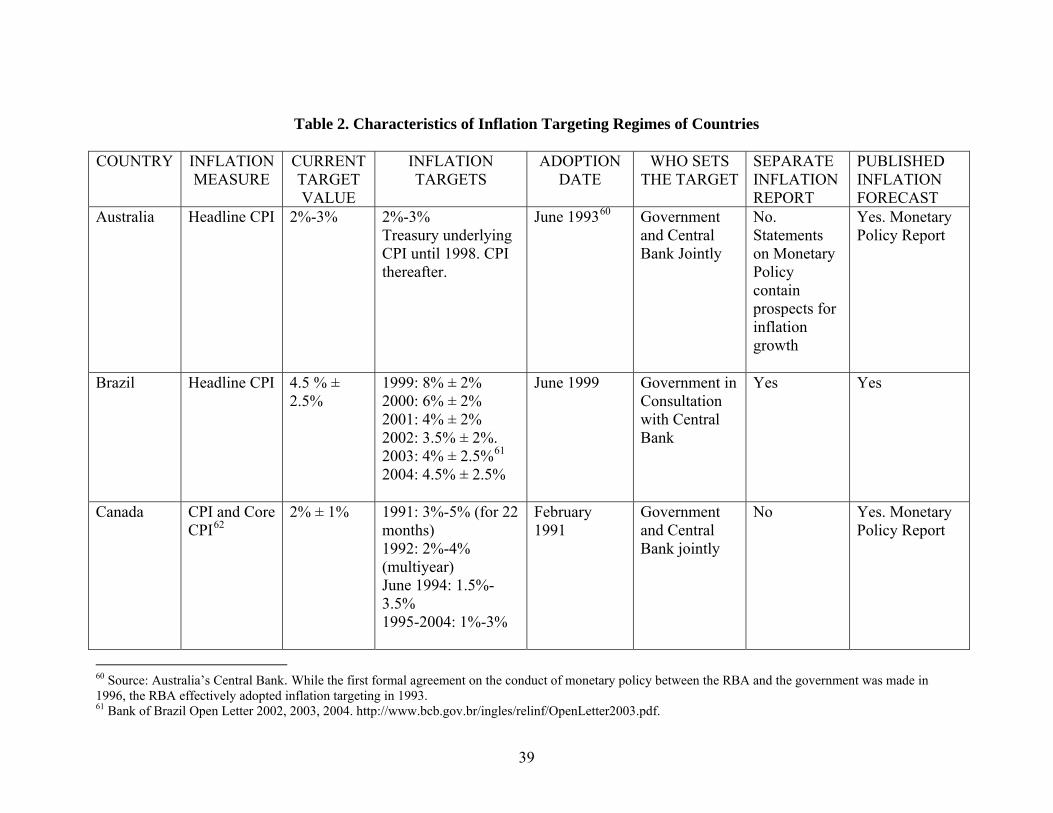
Table 2. Characteristics of Inflation Targeting Regimes of Countries
COUNTRY INFLATION
MEASURE CURRENT TARGET VALUE
INFLATION TARGETS
ADOPTION DATE
WHO SETS THE TARGET
SEPARATE INFLATION REPORT
PUBLISHED INFLATION FORECAST
Australia Headline CPI 2%-3% 2%-3% Treasury underlying CPI until 1998. CPI thereafter.
June 199360 Government and Central Bank Jointly
No. Statements on Monetary Policy contain prospects for inflation growth
Yes. Monetary Policy Report
Brazil Headline CPI 4.5 % ± 2.5%
1999: 8% ± 2% 2000: 6% ± 2% 2001: 4% ± 2% 2002: 3.5% ± 2%. 2003: 4% ± 2.5%61
2004: 4.5% ± 2.5%
June 1999 Government in Consultation with Central Bank
Yes Yes
Canada CPI and Core CPI62
2% ± 1%
1991: 3%-5% (for 22 months) 1992: 2%-4% (multiyear) June 1994: 1.5%-3.5% 1995-2004: 1%-3%
February 1991
Government and Central Bank jointly
No Yes. Monetary Policy Report
60 Source: Australia’s Central Bank. While the first formal agreement on the conduct of monetary policy between the RBA and the government was made in 1996, the RBA effectively adopted inflation targeting in 1993. 61 Bank of Brazil Open Letter 2002, 2003, 2004. http://www.bcb.gov.br/ingles/relinf/OpenLetter2003.pdf.
39

Chile Headline CPI
2%-4% 1991: 15%-20% 1992: 13%-16% 1993: 10%-12% 1994: 9%-11% 1995: 8% 1996: 6.5% 1997: 5.5% 1998: 4.5% 1999: 4.3% 2000: +/- 3.5% 2001, onward: 2%-4%
September 1990
Central Bank in consultation with Government
Yes Yes
Colombia CPI 6% 1999: 15% 2000: 10% 2001: 8% 2002: 6% 2003: 4%-6% 2004: 5%-6% 2005: 4.5% - 5.5% 2006: 3.5% – 5.5%
September 1999
Jointly by Government and Central Bank
Yes Yes
62 Canada’s Core CPI excludes food, energy, and the effect of indirect taxes.
40

Czech Republic
Net Inflation through 200163
Headline CPI thereafter
1%-3% Net Inflation 1998: 5.5% - 6.5 % 1999: 4%-5% 2000: 3.5% - 5.5. % 2001: 2%-4% Headline CPI 2002 –2005: Band starts Jan. 2002: 3%-5%. Band ends Dec. 2005: 2%-4% From 2006: 3%64
January 1998 Central Bank Yes Yes
Finland65 Core CPI NA Since 1993: 2% February 1993 to June 1998
Central Bank No No
Hungary CPI 4% ± 1% 2001: 7.5% ± 1% 2002: 4.5% ± 1% 2003: 3.5 % ± 1% 2004: 3.5 % ± 1% 2005: 4% ± 1% 2006: 3.5 % ± 1%
July 2001 Central Bank Yes Yes
63 Net inflation is calculated by the Czech Statistical Office (CSO) as the growth of prices in the unregulated part of the consumer basket adjusted for changes in indirect taxes and for abolition of subsidies. 64 The inflation target 3% has been announced for the period from Jan. 2006 until the Czech Republic’s accession to the euro area. 65 Since 1998, Finland has been a member of the ESCB and the Eurosystem.
41
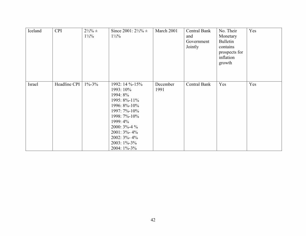
Iceland CPI 2½% ± 1½%
Since 2001: 2½% ± 1½%
March 2001 Central Bank and Government Jointly
No. Their Monetary Bulletin contains prospects for inflation growth
Yes
Israel Headline CPI 1%-3% 1992: 14 %-15% 1993: 10% 1994: 8% 1995: 8%-11% 1996: 8%-10% 1997: 7%-10% 1998: 7%-10% 1999: 4% 2000: 3%-4 % 2001: 3%- 4% 2002: 3%- 4% 2003: 1%-3% 2004: 1%-3%
December 1991
Central Bank Yes Yes
42

Korea CPI (1998) Core Inflation (after 1999)
2.5% - 3.5%
1998: 9 ± 1% 1999: 3 ± 1% 2000: 2.5 ± 1% 2001: 2.5 ± 1% 2002: 3 ± 1% 2003: 3 ± 1% Jan-2004, change to medium-term (instead of annual) targeting system. Target for 2004-2006: 2.5%-3.5%
April 1998 Government in Consultation with Central Bank
Yes Yes
Mexico Headline CPI 3% ± 1% 1999: 13% 2000: <10% 2001: 6.5% 2002: 4.5 % 2003: 3% ± 1% (in line with trading partners)
January 1999 Central Bank Yes Yes
New Zealand
Headline CPI66
1%-3% 1990: 3%-5% 1991: 2.5%-4.5% 1992: 1.5%- 3.5% 1993-1996: 0%-2% 1997-2001: 0%-3% 2002-present: 1%-3%
March 1990
Government and Central Bank jointly
Yes Yes
Norway CPI-ATE67 2.5% 2001-present: 2.5%
March 2001
Government Yes Yes
66 Officially CPI, but RBNZ targets "underlying" or "core" inflation.CPI: (since Dec-97, the CPI excluding credit services; before that date, overall CPI. In late 1999, mortgage interest rates were removed from the index)
43

Peru Headline CPI 2.5% ± 1% 1994: 15-20% 1995: 9-11% 1996: 9.5-11.5% 1997: 8-10% 1998: 7.5-9% 1999: 5-6% 2000: 3.5-4% 2001: 2.5-3.5% 2002: 2.5 ± 1% 2003: 2.5 ± 1% 2004: 2.5 ± 1%
January 1994 Central Bank in Consultation with Government
Yes Yes
Philippines CPI (they monitor Core CPI measures also)
4.5% - 5.5%
2002: 5%-6% 2003:4.5%-5.5% 2004: 4%-5% 2005: 4%-5%
January 2002 Jointly by Central Bank and Government
Yes Yes
Poland Headline CPI 2.5%± 1% 1998: <9.5% 1999: 6.6-7.8% 2000: 5.4-6.8% 2001:<6-8%. 3% by 2003 2002: 5% ± 1% <4% by 2003 2003: 3% ± 1% 2004: 2.5% ± 1%
October 1998 Central Bank Yes Yes
67 CPI inflation adjusted for tax changes and excluding energy products
44

South Africa
CPIX68 3%-6% 2003: 3%-6% February 2000
Government after consultation with the Reserve Bank and the National Treasury.
Yes No
Spain69 Headline CPI NA 1996: 3.5% - 4% 1997: 2.5% 1998: 2%
November 1994 to June 1998
Central Bank
Yes Yes
Sweden Headline CPI 2%± 1% Since 1995: 2% ± 1%
January 1993 Central Bank
Yes Yes
Switzerland Headline CPI Less than 2%
Since 2000: Less than 2%
January 2000 Central Bank No. Monetary Policy Report, Monetary Policy Assessment, and Inflation Forecast published quarterly
Yes
68 The consumer price index for metropolitan and other urban areas excluding the interest cost of mortgage bonds. 69 Since 1998, Spain is a member of the ESCB and the Eurosystem.
45
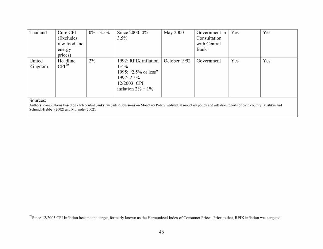
Thailand Core CPI (Excludes raw food and energy prices)
0% - 3.5% Since 2000: 0%-3.5%
May 2000 Government in Consultation with Central Bank
Yes Yes
United Kingdom
Headline CPI70
2% 1992: RPIX inflation 1-4% 1995: “2.5% or less” 1997: 2.5% 12/2003: CPI inflation 2% ± 1%
October 1992 Government Yes Yes
Sources: Authors’ compilations based on each central banks’ website discussions on Monetary Policy; individual monetary policy and inflation reports of each country; Mishkin and Schmidt-Hebbel (2002) and Morande (2002).
70Since 12/2003 CPI Inflation became the target, formerly known as the Harmonized Index of Consumer Prices. Prior to that, RPIX inflation was targeted.
46

TABLE 3. Effectiveness of Explicit Numeric Inflation Targeting
COUNTRY
Target Range as
of 12/2004
First Date for which Target
Range is not met
Number of
Periods within Range
Moving Average Rate of Inflation From Dec-2002
to Dec-2004
Standardized Deviation
from Moving Average
Australia 2 - 3 Jun-2000 17 2.51 0.02Brazil 4.5 ± 2.5 Dec-2003 12 8.80 1.72Canada 2 ± 1 Nov-1992 109 2.24 0.24Chile 2 - 4 Nov-2003 13 1.76 -1.24Colombia 5 - 6 Dec-2002 24 6.17 1.34Czech Republic
1 - 3 Feb-2002 34 1.93 -0.07
Hungary 3.5 ± 1 Dec-2003 12 5.75 2.25Iceland 2.5 ± 1.5 Aug-2003 (next
date is April 2001)
16 3.37 0.58
Israel 1 - 3 Nov-2003 13 -0.35 -2.35Korea 2.5 - 3.5 Nov-2003 (next
date is November
2001)
13 2.87 -0.26
Mexico 2 - 4 December 2003 12 4.69 1.69New Zealand 1 - 3 Never71 59 2.15 0.15Norway72 2.5 Never 45 0.85 ---Peru 2.5 ± 1 Nov-2003 13 3.03 0.53Philippines 4 - 5 Dec-2003 12 6.38 3.76Poland 2.5 ± 1.5 Dec-2003 12 3.09 0.39South Africa
3 - 6 Feb-2002 34 4.25 -0.17
Sweden 2 ± 1 Dec-2003 12 0.78 -1.22Switzerland Less than 2 Never73 59 0.97 -0.03Thailand 0 – 3.5 Never74 55 0.30 -0.83U.K. 2 ± 1 Never75 146 1.4676 -0.54
71 Average rate of Inflation for New Zealand never went outside the range since inflation targeting regime was adopted (1990). 72 No index numbers for CPI-ATE are available. Average rate of Headline CPI inflation was used instead. Value for average rate of Headline CPI inflation never exceeded 2.5 since inflation targeting regime was adopted (2001). 73 Average rate of inflation for Switzerland never went outside the range since inflation targeting regime was adopted (2000). First date for which the average rate of inflation was outside the range was Oct-89 at 2.09. 74 Average rate of inflation for Thailand never went outside the range since inflation targeting regime was adopted (2000). First date for which the average rate of inflation was outside the range was Aug-92 at 3.52. 75 First date for which the average rate of inflation was outside the range was Mar-92 at 3.03 for average rate of RPIX inflation. 76 Note that in 12/2002, UK targeted RPIX, and not Headline CPI. The value for the average rate of inflation of RPIX in 12/2002 was 2.6, still within the target range as of 12/2004.
47

Figure 1: Year of Adoption and Initial Inflation in Twenty Three Inflation-Targeting Countries
New Zealand
Chile
Canada
Israel
UK
Sweden Australia
KoreaPoland
Mexico
Brazil
South AfricaNorway
Czech Republic
Peru
Hungary
Colombia
Switzerland
Thailand
Iceland
Philippines
FinlandSpain
0
5
10
15
20
25
30
35
40
45
50
1988 1990 1991 1993 1994 1995 1997 1998 1999 2001 2002
Inflation (Percent)
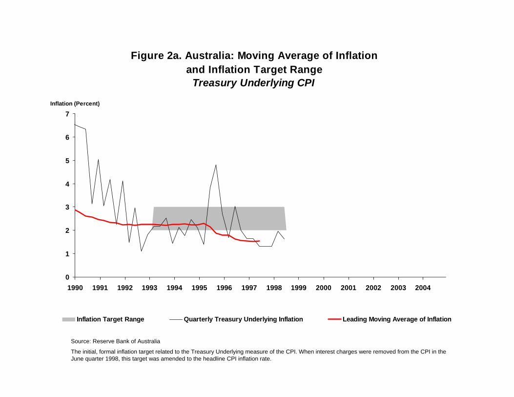
Figure 2a. Australia: Moving Average of Inflationand Inflation Target Range
Treasury Underlying CPI
0
1
2
3
4
5
6
7
1990 1991 1992 1993 1994 1995 1996 1997 1998 1999 2000 2001 2002 2003 2004
Inflation (Percent)
Inflation Target Range Quarterly Treasury Underlying Inflation Leading Moving Average of Inflation
Source: Reserve Bank of Australia
The initial, formal inflation target related to the Treasury Underlying measure of the CPI. When interest charges were removed from the CPI in the June quarter 1998, this target was amended to the headline CPI inflation rate.

Figure 2b. Australia: Moving Average of Inflationand Inflation Target Range
Headline CPI
-4
-2
0
2
4
6
8
10
12
14
16
1990 1991 1992 1993 1994 1995 1996 1997 1998 1999 2000 2001 2002 2003 2004
Inflation (Percent)
Inflation Target Range Quarterly Headline CPI Leading Moving Average of Inflation
Source: Reserve Bank of Australia
The initial, formal inflation target related to the Treasury Underlying measure of the CPI. When interest charges were removed from the CPI in the June quarter 1998, this target was amended to the headline CPI inflation rate.

Figure 3. Brazil: Moving Average of Inflation and Inflation Target Range
-20
-10
0
10
20
30
40
50
60
70
80
90
1990 1991 1992 1993 1994 1995 1996 1997 1998 1999 2000 2001 2002 2003 2004
Inflation (Percent)
Inflation Target Range Monthly Total CPI Inflation Leading Moving Average of Inflation
Source: Banco Central do Brazil
-5
0
5
10
15
20
25
30
35
40
2000 2001 2002 2003 2004
Inflation (Percent)

Figure 4. Canada: Moving Average of Inflation and Inflation Target Range
-15
-10
-5
0
5
10
15
20
25
30
35
1990 1992 1994 1996 1998 2000 2002 2004
Inflation (Percent)
Inflation Target Range Monthly Total CPI Inflation Leading Moving Average of Inflation
Source: Banque du Canada

Figure 5. Chile: Moving Average of Inflation and Inflation Target Range
-20
-10
0
10
20
30
40
50
60
70
1990 1992 1994 1996 1998 2000 2002 2004
Inflation (Percent)
Inflation Target Range Monthly Total CPI Inflation Target Midpoint Leading Moving Average of Inflation
Source: Banco Central de Chile
-10
-5
0
5
10
15
2000 2002 2004

Figure 6. Colombia: Moving Average of Inflation and Inflation Target Range
-10
0
10
20
30
40
50
60
1990 1992 1994 1996 1998 2000 2002 2004
Inflation (Percent)
Inflation Target Range Monthly Total CPI Inflation Target Midpoint Leading Moving Average of Inflation
Source: Banco Central de Colombia
-5
0
5
10
15
20
25
30
2000 2002 2004

Figure 7. Czech Republic: Moving Average of Inflation and Inflation Target Range
Headline CPI
-20
-10
0
10
20
30
40
50
60
1990 1991 1992 1993 1994 1995 1996 1997 1998 1999 2000 2001 2002 2003 2004
Inflation (Percent)
Inflation Target Range Monthly Total CPI Inflation Leading Moving Average of Inflation
Source: Czech Statistical Office
Czech Republic targeted Net inflation through 2001 and Headline CPI thereafter
-15
-10
-5
0
5
10
15
20
25
2000 2001 2002 2003 2004

Figure 8. Hungary: Moving Average of Inflation and Inflation Target Range
-10
0
10
20
30
40
50
60
70
80
90
1990 1991 1992 1993 1994 1995 1996 1997 1998 1999 2000 2001 2002 2003 2004
Inflation (Percent)
Inflation Target Range Monthly Total CPI Inflation Leading Moving Average of Inflation
Source: Hungarian Central Statistical Office
-10
-5
0
5
10
15
20
25
30
2000 2001 2002 2003 2004 2005

Figure 9. Iceland: Moving Average of Inflation and Inflation Target Range
-10
-5
0
5
10
15
20
25
1990 1991 1992 1993 1994 1995 1996 1997 1998 1999 2000 2001 2002 2003 2004 2005
Inflation (Percent)
Inflation Target Range Monthly Total CPI Inflation Leading Moving Average of Inflation
Source: Statistics Iceland

Figure 10. Israel: Moving Average of Inflation and Inflation Target Range
-20
-10
0
10
20
30
40
1990 1991 1992 1993 1994 1995 1996 1997 1998 1999 2000 2001 2002 2003 2004
Inflation (Percent)
Inflation Target Range Monthly Total CPI Inflation Target Midpoint Leading Moving Average of Inflation
Source: Central Bureau of Statistics, Israel

Figure 11a. Korea: Moving Average of Inflation and Inflation Target Range
Total CPI Inflation
-10
-5
0
5
10
15
20
25
30
35
1990 1991 1992 1993 1994 1995 1996 1997 1998 1999 2000 2001 2002 2003 2004
Inflation (Percent)
Inflation Target Range Monthly Total CPI InflationTarget Midpoint Leading Moving Average of Inflation
Source: Korea National Statistics Office and The Bank of Korea.
Total CPI was targeted until 1999. Core Inflation was targeted beginning in 2000.

Figure 11b. Korea: Moving Average of Inflation and Inflation Target Range
Core CPI Inflation
-5
0
5
10
15
20
25
30
1990 1991 1992 1993 1994 1995 1996 1997 1998 1999 2000 2001 2002 2003 2004
Inflation (Percent)
Inflation Target Range Monthly Core CPI Inflation Target Midpoint Leading Moving Average of Inflation
Source: Korea National Statistics Office and The Bank of Korea.
Total CPI was targeted until 1999. Core Inflation was targeted beginning in 2000.
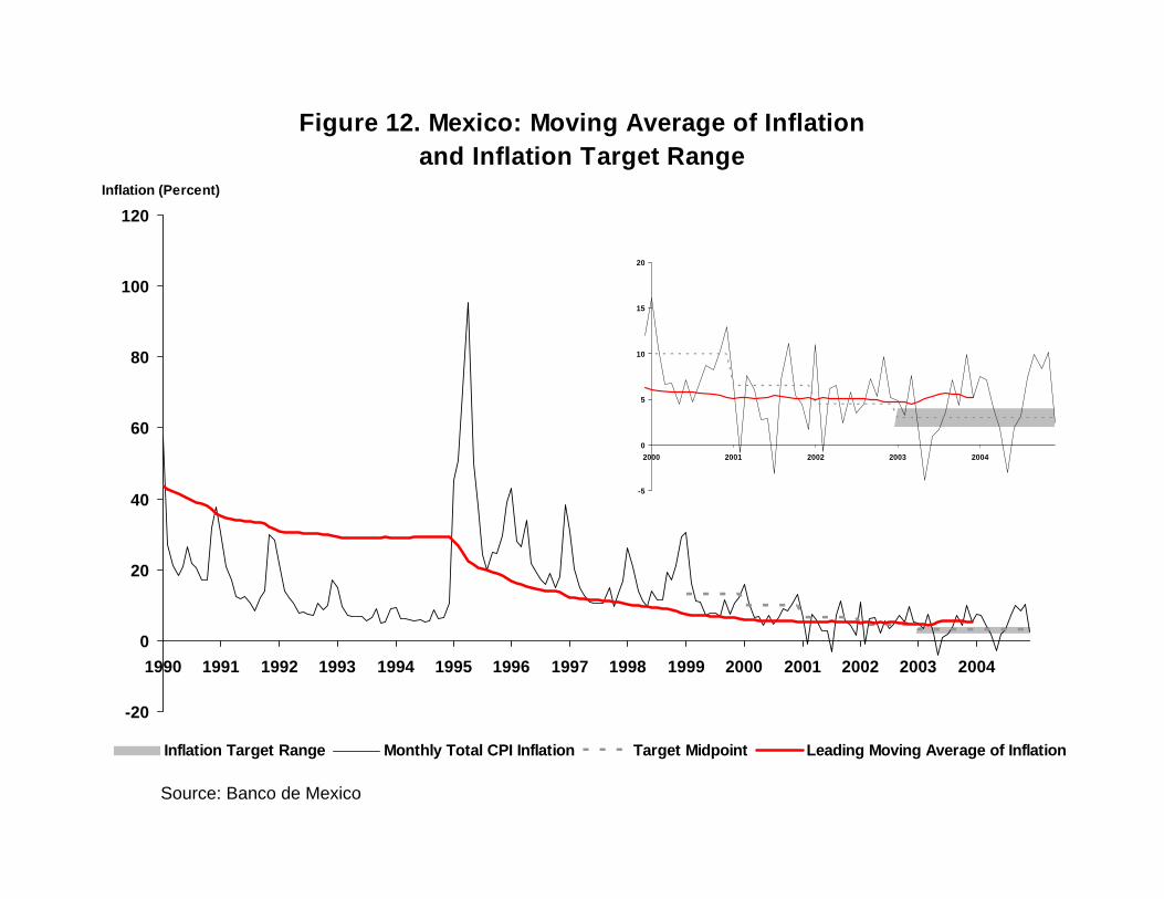
Figure 12. Mexico: Moving Average of Inflation and Inflation Target Range
-20
0
20
40
60
80
100
120
1990 1991 1992 1993 1994 1995 1996 1997 1998 1999 2000 2001 2002 2003 2004
Inflation (Percent)
Inflation Target Range Monthly Total CPI Inflation Target Midpoint Leading Moving Average of Inflation
Source: Banco de Mexico
-5
0
5
10
15
20
2000 2001 2002 2003 2004
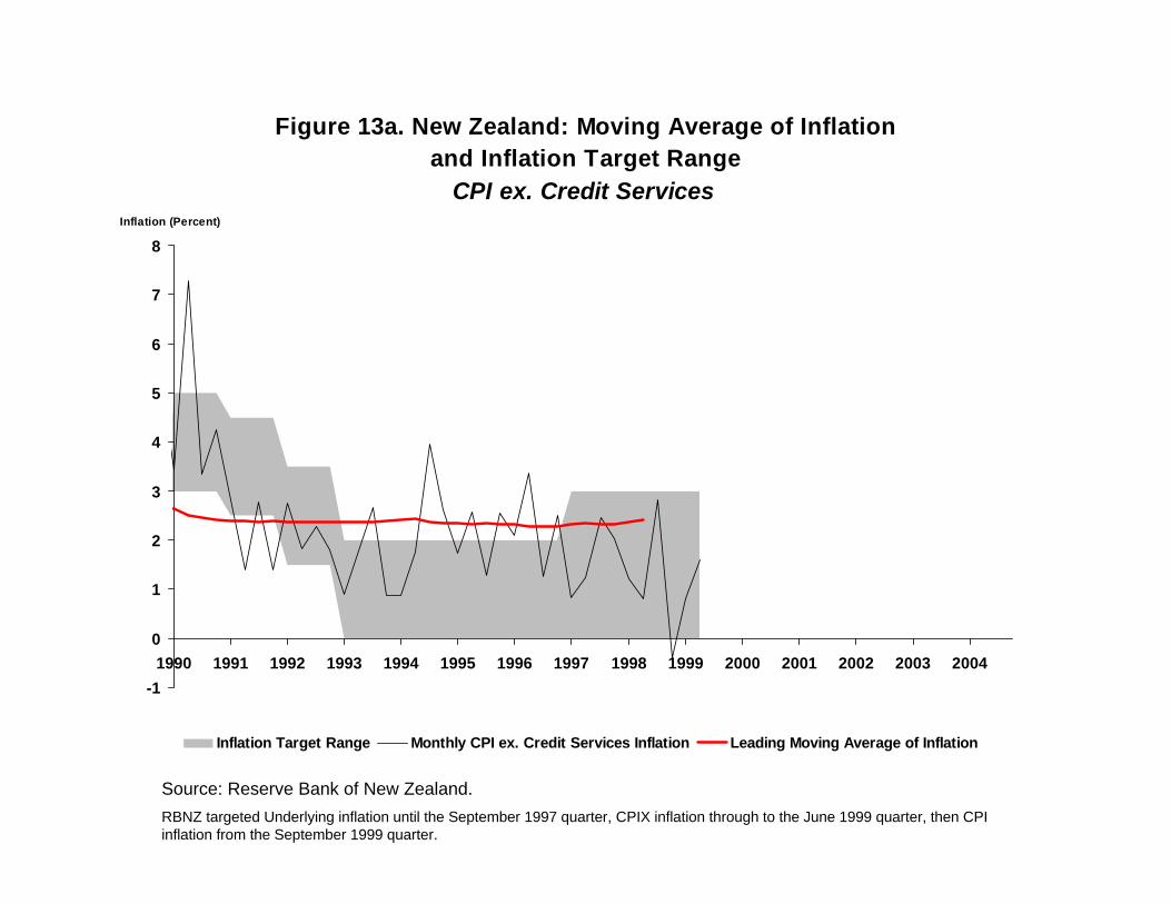
Figure 13a. New Zealand: Moving Average of Inflation and Inflation Target Range
CPI ex. Credit Services
-1
0
1
2
3
4
5
6
7
8
1990 1991 1992 1993 1994 1995 1996 1997 1998 1999 2000 2001 2002 2003 2004
Inflation (Percent)
Inflation Target Range Monthly CPI ex. Credit Services Inflation Leading Moving Average of Inflation
Source: Reserve Bank of New Zealand.RBNZ targeted Underlying inflation until the September 1997 quarter, CPIX inflation through to the June 1999 quarter, then CPI inflation from the September 1999 quarter.

Figure 13b. New Zealand: Moving Average of Inflation and Inflation Target Range
Headline CPI
-4
-2
0
2
4
6
8
1990 1991 1992 1993 1994 1995 1996 1997 1998 1999 2000 2001 2002 2003 2004
Inflation (Percent)
Inflation Target Range Monthly Total CPI Inflation Leading Moving Average of Inflation
Source: Reserve Bank of New Zealand.
RBNZ targeted Underlying inflation until the September 1997 quarter, CPIX inflation through to the June 1999 quarter, then CPI inflation from the September 1999 quarter.

Figure 14. Norway: Moving Average of Inflation and Inflation Target Range
-20
-15
-10
-5
0
5
10
15
20
25
30
35
1990 1991 1992 1993 1994 1995 1996 1997 1998 1999 2000 2001 2002 2003 2004
Inflation (Percent)
Total CPI Inflation Target Leading Moving Average of Inflation
Source: Statistics Norway

Figure 15. Peru: Moving Average of Inflation and Inflation Target Range
-20
0
20
40
60
80
100
1990 1992 1994 1996 1998 2000 2002 2004
Inflation (Percent)
Inflation Target Range Monthly Total CPI Inflation Leading Moving Average of Inflation
Source: Central Reserve Bank of Peru.
-10
-5
0
5
10
15
2000 2001 2002 2003 2004

Figure 16. Philippines: Moving Average of Inflationand Inflation Target Range
-50
-30
-10
10
30
50
70
90
1990 1992 1994 1996 1998 2000 2002 2004
Inflation (Percent)
Inflation Target Range Monthly Total CPI Target Midpoint Leading Moving Average of Inflation
Source: Central Bank of Philippines.
-5
0
5
10
15
20
25
2000 2001 2002 2003 2004 2005

Figure 17. Poland: Moving Average of Inflation and Inflation Target Range
-20
0
20
40
60
80
100
120
140
160
180
1990 1992 1994 1996 1998 2000 2002 2004
Inflation (Percent)
Inflation Target Range Monthly CPI Inflation Midpoint Leading Moving Average of Inflation
Source: Central Statistical Office, Poland
-10
-5
0
5
10
15
20
25
2000 2002 2004
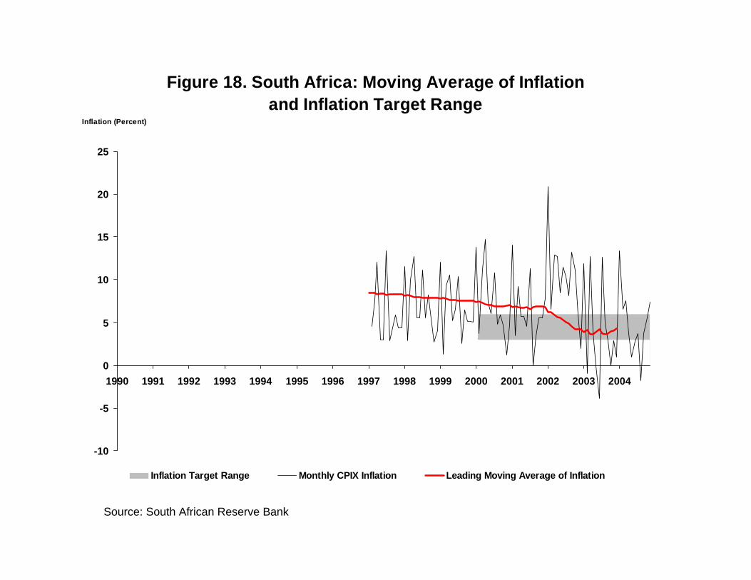
Figure 18. South Africa: Moving Average of Inflation and Inflation Target Range
-10
-5
0
5
10
15
20
25
1990 1991 1992 1993 1994 1995 1996 1997 1998 1999 2000 2001 2002 2003 2004
Inflation (Percent)
Inflation Target Range Monthly CPIX Inflation Leading Moving Average of Inflation
Source: South African Reserve Bank

Figure 19. Sweden: Moving Average of Inflation and Inflation Target Range
-20
-10
0
10
20
30
40
50
1990 1992 1994 1996 1998 2000 2002 2004
Inflation (Percent)
Inflation Target Range Monthly Total CPI Inflation Leading Moving Average of Inflation
Source: Statistics Sweden
-15
-10
-5
0
5
10
15
2000 2001 2002 2003 2004

Figure 20. Switzerland: Moving Average of Inflation and Inflation Target Range
-15
-10
-5
0
5
10
15
20
1990 1992 1994 1996 1998 2000 2002 2004
Inflation (Percent)
Inflation Target Range Monthly Total CPI Inflation Leading Moving Average of Inflation
Source: Swiss National Bank

Figure 21. Thailand: Moving Average of Inflation and Inflation Target Range
-10
-5
0
5
10
15
20
1990 1992 1994 1996 1998 2000 2002 2004
Inflation (Percent)
Inflation Target Range Monthly Core CPI Inflation Leading Moving Average of Inflation
Source : Bureau of Trade and Economic Indices, Ministry of Commerce, Thailand

Figure 22a. United Kingdom: Moving Average of Inflation and Inflation Target Range
RPIX
-20
-10
0
10
20
30
40
50
1990 1991 1992 1993 1994 1995 1996 1997 1998 1999 2000 2001 2002 2003 2004
Inflation (Percent)
RPIX Inflation Target Range RPIX Lower Bound Monthly RPIX Inflation Leading Moving Average of Inflation
Source: National Statistics, UK
* Since Dec. 2003, the UK's inflation target has been based on the Consumer Prices Index
-10
-8
-6
-4
-2
0
2
4
6
8
10
12
2000 2001 2002 2003 2004
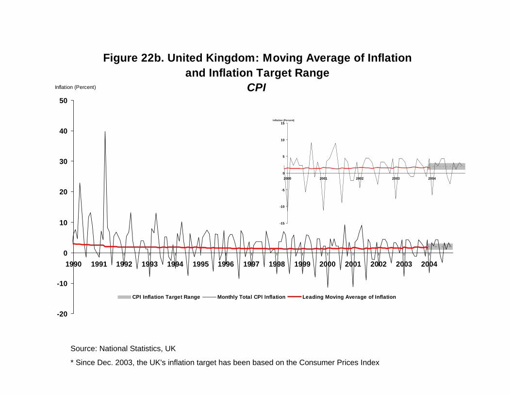
Figure 22b. United Kingdom: Moving Average of Inflation and Inflation Target Range
CPI
-20
-10
0
10
20
30
40
50
1990 1991 1992 1993 1994 1995 1996 1997 1998 1999 2000 2001 2002 2003 2004
Inflation (Percent)
CPI Inflation Target Range Monthly Total CPI Inflation Leading Moving Average of Inflation
Source: National Statistics, UK
* Since Dec. 2003, the UK's inflation target has been based on the Consumer Prices Index
-15
-10
-5
0
5
10
15
2000 2001 2002 2003 2004
Inflation (Percent)

Figure 23a. United States: Moving Average of Inflation and Inflation Range
Core CPI
0
1
2
3
4
5
6
7
8
9
1990 1991 1992 1993 1994 1995 1996 1997 1998 1999 2000 2001 2002 2003 2004 2005
Inflation (Percent)
Inflation Range Monthly Core CPI Inflation Leading Moving Average of Inflation
Source: FRED Economic Database. Consumer Price Index for All Urban Consumers: All Items Less Food & Energy

Figure 23b. United States: Moving Average of Inflation and Inflation Range
Core PCE
-8
-6
-4
-2
0
2
4
6
8
10
12
1990 1991 1992 1993 1994 1995 1996 1997 1998 1999 2000 2001 2002 2003 2004 2005
Inflation (Percent)
1-3 Percent Inflation Range Monthly Core PCE Inflation Leading Moving Average of Inflation

Figure 24. U.S. Housing StartsAnnual Rates
0
500
1000
1500
2000
2500
3000
1959 1962 1965 1968 1971 1974 1977 1980 1983 1986 1989 1992 1995 1998 2001 2004
Thousands of Units
Top Related