


Languages
Pages
Legal


General rights Copyright and moral rights for the publications made accessible in the public portal are retained by the authors and/or other copyright owners and it is a condition of accessing publications that users recognise and abide by the legal requirements associated with these rights.
• Users may download and print one copy of any publication from the public portal for the purpose of private study or research. • You may not further distribute the material or use it for any profit-making activity or commercial gain • You may freely distribute the URL identifying the publication in the public portal
If you believe that this document breaches copyright please contact us providing details, and we will remove access to the work immediately and investigate your claim.
Downloaded from orbit.dtu.dk on: Dec 18, 2017
The effect of microscale spatial variability of wind on estimation of technical andeconomic wind potential
Balyk, Olexandr; Badger, Jake; Karlsson, Kenneth Bernard
Publication date:2015
Link back to DTU Orbit
Citation (APA):Balyk, O., Badger, J., & Karlsson, K. B. (2015). The effect of microscale spatial variability of wind on estimationof technical and economic wind potential. Paper presented at 34th edition of the International Energy Workshop,Abu Dhabi, United Arab Emirates.
brought to you by COREView metadata, citation and similar papers at core.ac.uk
provided by Online Research Database In Technology

Theeffectofmicroscalespatialvariabilityofwindonestimationoftechnicalandeconomicwindpotential
Olexandr Balyka*, Jake Badgerb, Kenneth Karlssona
Affiliation: a DTU Management Engineering, b DTU Wind Energy. Both are part of Technical University
of Denmark, P.O. Box 49, DK‐4000 Roskilde, Denmark;
* Corresponding author. Mailing address: P.O. Box 49, 4000 Roskilde, Denmark; telephone number:
+45 4677 5123; fax number: +45 4677 5199; e‐mail: [email protected]
AbstractThis study presents a novel methodology for estimating wind energy potential using high resolution
wind atlas data. The data captures microscale spatial wind variability effects and results in a higher
potential than lower resolution wind resource data. Compared to upscaled wind resource data
(simulated coarse mesoscale data with a grid spacing of 30km), economic wind energy potential
estimated in the test area using microscale data with a 250m spacing is at least twice as high.
In order to estimate the gross technical wind energy potential in the test area, for the first time the
high resolution annual wind climate data is transformed into yearly average energy production using
a wind turbine power curve. Later on, detailed land availability data is combined with assumptions
on wind turbine spacing and economic feasibility to aid the estimation of the net technical and
economic wind potentials. To account for realistic turbine spacing we present a novel application of
binary integer programming and compare it to two simpler approaches (i.e. maxim and average
value approaches).
The developed methodology has a number of interesting implications for energy system analysis
studies in general and integrated assessment modelling in particular; namely, more realistic wind
potential estimates, higher competitiveness of wind energy, and an increased climate change
mitigation potential.
In anticipation of the release of global high resolution wind climate data, the developed
methodology can be extended to provide estimates of technical and economic wind energy potential
regionally or globally.
Keywords: high resolution wind resource, wind atlas, AEP, technical and economic potential
1 IntroductionWind energy can play an important role in climate change mitigation, reduction of local air pollution
and reducing dependence on fossil fuels. However its exact future role remains largely uncertain.
One of the reasons behind this is the uncertainty about wind potential available regionally and
globally, as well as cost at which it can be deployed. Researchers around the world agree that
reducing this uncertainty will benefit energy planning in general and climate change mitigation
studies in particular [1‐4].

There have been a number of studies looking at the global wind energy potential. Hoogwijk et al. [5]
use monthly wind speed data from the Climate Research Unit (CRU) to estimate global onshore wind
energy potential on a 0.5° 0.5° grid. Archer and Jacobson [6] rely an average yearly wind speed derived from over 8000 surface and sounding stations to come up with both onshore and offshore
wind potential. Lu et al. [7] base their estimate on wind speed data with the spatial resolution of
1 2⁄ ° longitude by 2 3⁄ ° latitude and temporal resolution of 6 hours from the Goddard Earth
Observing System Data Assimilation System. Zhou et al. [8] make use of Climate Forecast System
Reanalysis (CFSR) hourly wind speed data with a spatial resolution of 0.3125° latitude/longitude. These studies produce estimates exceeding by far current global electricity demand; however these
studies use spatial resolution which is unable to resolve the kinds of terrain features which are the
preferred sites for wind turbine placement in practice. This limitation is noted by, e. g. Zhou et al.
[8].
There also have been many studies focusing on wind energy potential on the regional level [9‐14].
Normally they rely on higher resolution wind data and utilise more complex estimation techniques
than the global studies. Despite this, they present challenges for global analyses due to limited
regional coverage, as well as inconsistent underlying assumptions and estimation techniques.
Making detailed wind resource maps globally would be very time consuming as it this would require
more local measurements, unless the microscale wind climate could be captured by downscaling
existing mesoscale wind data.
The Global Wind Atlas (GWA) project1 represents such an effort. One of its goals is to provide a
consistent, publicly available dataset with a global coverage. The method [15, 16] for the GWA
project is being validated on several test areas. One of them is a test area in the US, situated in the
states of Washington and Oregon (Figure 1). The region is characterised by drastic changes in
elevation and land use that make it a good test area for wind resource assessment. A preliminary
dataset using the GWA method is used in the present study.
Figure 1 – Geographical location of the test area.
This study has several purposes. One of them is to showcase a new methodology for estimating wind
energy potential using GWA data. Although high resolution wind climate data has been used before
1 Project funded by grant EUDP 11‐II, Globalt Vind Atlas, 64011‐0347.

to estimate wind power density [17], an estimation resulting in annual energy production (AEP) has
not been demonstrated. We use binary integer programming among other approaches to convert
the resulting high resolution AEP map to technical and economic potential. Previously optimisation
methods have been limited to wind farm layout optimisation [18‐20], here we apply it for optimal
wind turbine siting over a large region.
Another purpose of the study is to provide an indication of how high resolution wind data influences
the estimated wind energy potential. In order to achieve the latter, a comparison is made with
calculations using simulated mesoscale data. Up to date this is the first attempt to calculate impact
of resolution effect on technical and economic potential in this way. In addition, implications for
reaching a certain capacity of installed wind power are presented.
Phadke et al. [21] is an example of a study which gave a revised estimate of technical wind potential
in India based on an increased area available for deployment of wind energy derived from high
resolution land use data. In this study we go one step further with our methodology which can use
land use data and wind climate data both at high resolution.
2 MethodologyThe methodology used in this study can be broken down into a number of steps. The following
subsections provide further details on the steps and data used.
2.1 MicroscaledataFor the purpose of this study we use wind resource data estimated during the development of the
GWA methodology. It is based on NCEP DOE II reanalysis data [22] applied in a microscale modelling
system based on WAsP2. The 100m above surface level annual wind climate data is given in terms
of Weibull distributions describing the wind speed distribution for 12 direction sectors. The data consists of:
‐ Weibull parameter k by sector;
‐ Weibull parameter A by sector;
‐ Sector frequency.
The data has a spatial resolution of 250 meters.
2.2 WindspeeddistributionWe start with the cumulative distribution function for the Weibull distribution (Equation (1)) and
then estimate probabilities for different wind speed intervals for each sector and in each grid cell
(Equation (2)).
, 1 ⁄ (1) Where , is probability of wind speed less or equal to in sector ; and are Weibull
parameters.
2 WAsP (or Wind Atlas Analysis and Application Program) is a software package for wind data analysis, wind climate estimation, and siting of wind turbines.

, , , , (2) Where , , is probability of wind speed between and in sector .
The wind speed intervals are dimensioned corresponding to the power curve data (i.e. 1 / ) used
in the next step.
2.3 GrosstechnicalwindenergypotentialHere we estimate gross technical wind energy potential. This is wind energy that could be produced
by wind turbines without taking into account any siting constraints. For this study we use the power
curve of a Vestas V90 3MW turbine [23]. We assume that every 250 250m grid cell can
potentially be occupied by one turbine.
In order to arrive at the potential, first we estimate average power generation for each sector
(Equation (3)) based on the power curve and probabilities obtained in Equation (2).
, , 2⁄ (3)
Where ) is average power generation for sector and 2⁄ is wind turbine
power output at wind speed 2⁄ .
Then we use the sector frequency data to estimate omnidirectional average power generation
(Equation (4)).
(4)
Where is frequency of sector .
Finally, we estimate annual energy production (AEP) by multiplying the result of Equation (4) by the
number of hours in a year (Equation (5)).
8766 (5)
2.4 AreaexclusionSome areas are not suitable for wind power development due to their physical characteristics (e.g.
slope), management practice (e.g. protected areas), etc. Therefore, in order to obtain a more
realistic estimate of wind energy potential, it is important to identify those areas and exclude them
from the available land for wind power development.
As an example, we use a publically available dataset which includes protected areas of the Pacific
States [24]. Protected areas in this dataset are classified according to the International Union for
Conservation of Nature (IUCN) protected areas categories that include: strict nature reserves,
wilderness areas, national parks, natural monuments, habitat/species management areas, protected
landscape/seascape areas and managed resource protected areas. The dataset also contains
protected areas for which primary management objective is unknown.
More areas could be considered as not suitable including cities, roads, areas with high slopes and
long distance to power grid, etc. before using the estimated potential in planning or energy system
modelling. This has not been done in this paper as the focus is on developing a methodology, for
which the used exclusion constraint perfectly serves the purpose.

2.5 ApproachestoestimateanettechnicalpotentialThe gross technical potential assumed a turbine in every grid cell. In practice wind turbines of the
size being considered in this study would not be placed so densely. This is because wakes downwind
of wind turbines reduce the wind speed and increase the turbulence, both of which are unattractive
for turbine siting. Therefore it is important to consider a more realistic spacing of turbines, which
reduces the effects of wakes and provides more realistic potential.
Therefore, here we assume a turbine density of 1 turbine per km , which is equivalent to a spacing
of about 11 rotor diameters.
In the following we consider three different methods of calculating the net technical potential taking
into account the assumed turbine density.
2.5.1 MaximumvalueapproachThe whole test area is subdivided into 1km grid cell arrays (i.e. corresponding to the assumed
turbine density), with each array consisting of 4 4 grid cells. The grid cell with the maximum AEP
value is taken as a representative for the whole array. Naturally, those grid cells which are not
suitable for wind turbine placement (as determined by the exclusion criteria listed in Section 2.4) are
considered with zero AEP.
2.5.2 AveragevalueapproachIn this approach the average AEP value is calculated for each 1km grid cell array. All other
considerations remain unchanged. However, in order to avoid artificially low values in those arrays
where some of the grid cells fall under exclusion criteria, those grid cells are not taken into account.
Namely, the average AEP is calculated based only on the grid cells which are suitable for wind
turbine placement.
2.5.3 BinaryintegerprogrammingapproachThe binary integer programming (BIP) approach ensures that a particular turbine density is
maintained for an arbitrary selected grid cell array (i.e. area is not subdivided into rigid arrays as
before). So a randomly positioned 1km grid cell array will never have more than one turbine in it.
In order to estimate maximum AEP from the area, given a wind turbine spacing, the following
problem is solved.
→ (6)
Subject to the following constraints:
1∀ ∈ 1,2,3, … , 1 , ∀ ∈ 1,2,3, … , 1
∈ 0,1 ∀ ∈ 1,2,3, … , , ∀ ∈ 1,2,3, … ,
(7)
Where is the number of grid cells from east to west, is the number of grid cells from north to
south, and is the spacing coefficient.
These constrains ensure that for a given array only one grid cell can be occupied by a turbine. In the
optimal solution any given variable will be either 1 or 0, indicating whether the grid cell , is
occupied 1 by wind turbine or not 0 .
Due to computational intensity the whole area is split into subareas of 50 50km size. These are
then solved independently in a consecutive manner.
2.6 EconomicpotentialEconomic potential is the technical potential that is economically feasible to develop. There are
many factors that can influence the cost of development of a particular wind energy project.
In order to simplify the comparison we exclude grid cells with capacity factor lower than 0.35. We
then carry out calculations described in section 2.5, i.e. we use the maximum, average and BIP
approach to arrive at the economic potential.
2.7 ComparisonwithmesoscaledataIn order to illustrate advantages of microscale data, we need to compare our results to results
corresponding to those which would be obtained from coarse mesoscale data. In order to simulate
effects of mesoscale data, we average AEP values for the grid cell with a spacing of 30km
corresponding to the resolution commonly used in global wind potential studies. This simulated
mesoscale data will probably overestimate the wind resource calculated from actual mesoscale data,
as the increased resource contributions from high resolution terrain will exceed decreased resource
contribution from high resolution terrain [15].
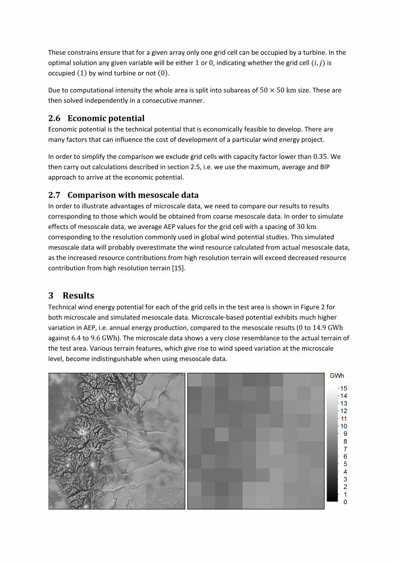
3 ResultsTechnical wind energy potential for each of the grid cells in the test area is shown in Figure 2 for
both microscale and simulated mesoscale data. Microscale‐based potential exhibits much higher
variation in AEP, i.e. annual energy production, compared to the mesoscale results (0 to 14.9GWh against 6.4 to 9.6GWh). The microscale data shows a very close resemblance to the actual terrain of
the test area. Various terrain features, which give rise to wind speed variation at the microscale
level, become indistinguishable when using mesoscale data.

Figure 2 – Variation in AEP calculated with microscale (left) and simulated mesoscale (right) data. Resolution: microscale
and simulated mesoscale.
A ‘summarising’ comparison is shown in Figure 3. For the purpose of comparing, each of the
mesoscale grid cells is divided into smaller grid cells to match the resolution of the microscale data.
The AEP value is duplicated within the same mesoscale grid cell. Figure 3 (left) illustrates mean AEP
for various number of grid cells. The difference between microscale‐ and mesoscale‐derived mean
AEP is about 20% for the 5% of the grid cells with the highest AEP values. This difference decreases
with the increasing number of the grid cells (e.g. to 14% for the 10% of the grid cells with the
highest AEP) until it becomes zero when all of the grid cells are considered. Since every microscale‐
and mesoscale‐derived mean AEP in this comparison is based on the grid cells with the highest AEP,
the grid cells giving rise to a particular pair of the microscale‐ and mesoscale‐derived mean AEP do
not necessarily represent the same geographical location.
Figure 3 – Left: microscale‐ and mesoscale‐derived cumulative moving mean AEP for various number of grid cells; the mean is based on
data sorted in descending order, therefore the mean values corresponding to the same number of grid cells do not necessarily
represent the same geographical area. Right: microscale‐derived AEP plotted against mesoscale‐derived AEP for every grid cell; the
dashed line represents mesoscale‐derived AEP plotted against itself (this shows variation of the microscale‐derived AEP within a
mesoscale grid cell).
Figure 3 (right) represents a comparison of mesoscale‐ and microscale‐derived AEP for every
microscale grid cell. It also illustrates the variation of microscale‐derived AEP within a mesoscale grid
cell (i.e. vertical variation along the dashed line). Here one can see that the corresponding
microscale value for a specific grid cell can be twice as high as the mesoscale value. This is true for
the grid cells with very good wind resources. Whereas some of the grid cells with poor wind
resources exhibit high mesoscale values.
Figure 4 illustrates results of using the different data and approaches for estimating the net technical
wind potential. It shows the percentage of the grid cells that can be occupied in the test area (given
the density of 1 turbine per km and the availability of the area) and the corresponding capacity
factor of the marginal turbine. Here the BIP approach is the only approach which ensures that in
addition to the maximum density a certain minimum distance is maintained between the turbines.
Under this approach the smallest fraction of grid cells, i.e. 4.3%, constitute the net technical
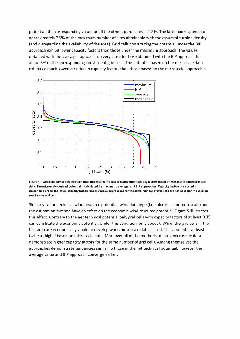
potential; the corresponding value for all the other approaches is 4.7%. The latter corresponds to
approximately 75% of the maximum number of sites obtainable with the assumed turbine density
(and disregarding the availability of the area). Grid cells constituting the potential under the BIP
approach exhibit lower capacity factors than those under the maximum approach. The values
obtained with the average approach run very close to those obtained with the BIP approach for
about 3% of the corresponding constituent grid cells. The potential based on the mesoscale data
exhibits a much lower variation in capacity factors than those based on the microscale approaches.
Figure 4 – Grid cells comprising net technical potential in the test area and their capacity factors based on mesoscale and microscale
data. The microscale‐derived potential is calculated by maximum, average, and BIP approaches. Capacity factors are sorted in
descending order; therefore capacity factors under various approaches for the same number of grid cells are not necessarily based on
exact same grid cells.
Similarly to the technical wind resource potential, wind data type (i.e. microscale or mesoscale) and
the estimation method have an effect on the economic wind resource potential. Figure 5 illustrates
this effect. Contrary to the net technical potential only grid cells with capacity factors of at least 0.35 can constitute the economic potential. Under this condition, only about 0.8% of the grid cells in the
test area are economically viable to develop when mesoscale data is used. This amount is at least
twice as high if based on microscale data. Moreover all of the methods utilising microscale data
demonstrate higher capacity factors for the same number of grid cells. Among themselves the
approaches demonstrate tendencies similar to those in the net technical potential; however the
average value and BIP approach converge earlier.

Figure 5 – Grid cells comprising economic potential in the test area their capacity factors based on mesoscale and microscale data. The
microscale‐derived potential is calculated by maximum, average, and BIP approaches. Capacity factors are sorted in descending order;
therefore capacity factors under various approaches for the same number of grid cells do not necessarily represent the same
geographical area.
Figure 6 gives some insight into the difference between technical and economic potential estimated
using the BIP approach. There the economic potential constitutes close to 37% of the technical
potential in terms of the number of sites. However for the same number of grid cells the capacity
factor of the economic potential is slightly higher.
Figure 6 – Technical and economic potential based on microscale data and calculated using BIP approach. Capacity factors are sorted in
descending order; therefore capacity factors for technical and economic potential for the same number of grid cells do not necessarily
represent the same geographical area.
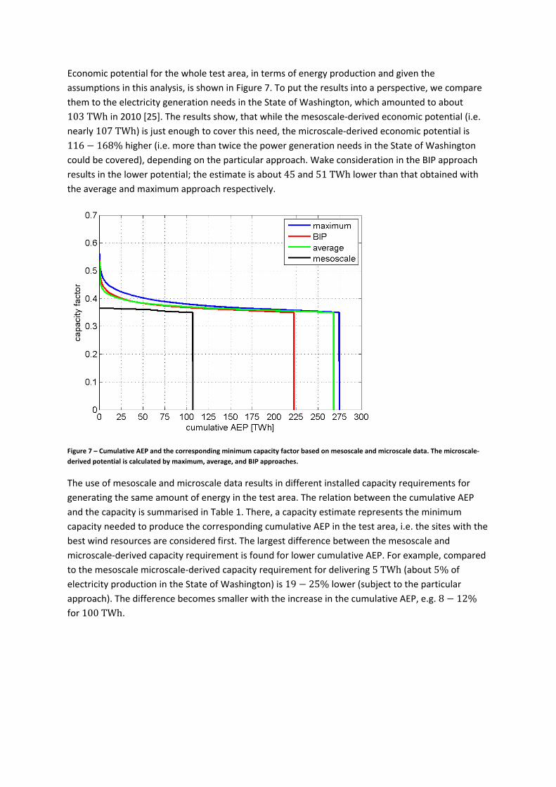
Economic potential for the whole test area, in terms of energy production and given the
assumptions in this analysis, is shown in Figure 7. To put the results into a perspective, we compare
them to the electricity generation needs in the State of Washington, which amounted to about
103TWh in 2010 [25]. The results show, that while the mesoscale‐derived economic potential (i.e.
nearly 107TWh) is just enough to cover this need, the microscale‐derived economic potential is
116 168% higher (i.e. more than twice the power generation needs in the State of Washington
could be covered), depending on the particular approach. Wake consideration in the BIP approach
results in the lower potential; the estimate is about 45 and 51TWh lower than that obtained with the average and maximum approach respectively.
Figure 7 – Cumulative AEP and the corresponding minimum capacity factor based on mesoscale and microscale data. The microscale‐
derived potential is calculated by maximum, average, and BIP approaches.
The use of mesoscale and microscale data results in different installed capacity requirements for
generating the same amount of energy in the test area. The relation between the cumulative AEP
and the capacity is summarised in Table 1. There, a capacity estimate represents the minimum
capacity needed to produce the corresponding cumulative AEP in the test area, i.e. the sites with the
best wind resources are considered first. The largest difference between the mesoscale and
microscale‐derived capacity requirement is found for lower cumulative AEP. For example, compared
to the mesoscale microscale‐derived capacity requirement for delivering 5TWh (about 5% of
electricity production in the State of Washington) is 19 25% lower (subject to the particular
approach). The difference becomes smaller with the increase in the cumulative AEP, e.g. 8 12%
for 100TWh.
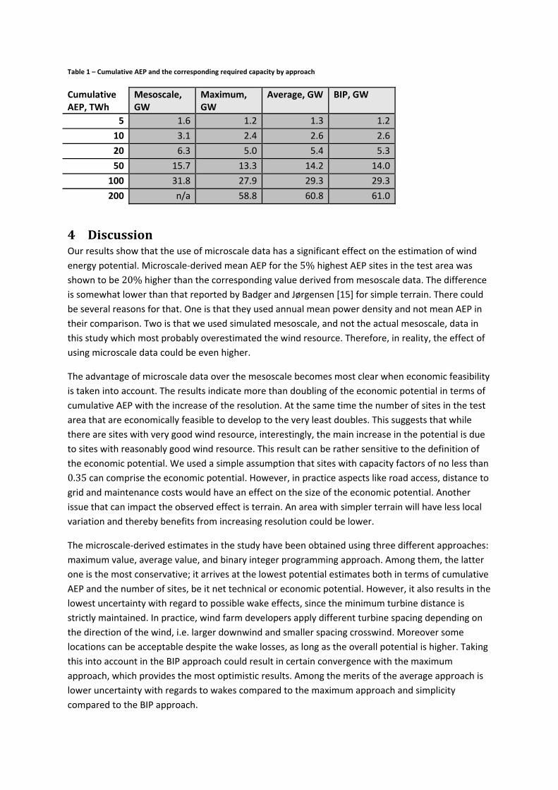
Table 1 – Cumulative AEP and the corresponding required capacity by approach
Cumulative AEP, TWh
Mesoscale, GW
Maximum, GW
Average, GW BIP, GW
5 1.6 1.2 1.3 1.2
10 3.1 2.4 2.6 2.6
20 6.3 5.0 5.4 5.3
50 15.7 13.3 14.2 14.0
100 31.8 27.9 29.3 29.3
200 n/a 58.8 60.8 61.0
4 DiscussionOur results show that the use of microscale data has a significant effect on the estimation of wind
energy potential. Microscale‐derived mean AEP for the 5% highest AEP sites in the test area was
shown to be 20% higher than the corresponding value derived from mesoscale data. The difference
is somewhat lower than that reported by Badger and Jørgensen [15] for simple terrain. There could
be several reasons for that. One is that they used annual mean power density and not mean AEP in
their comparison. Two is that we used simulated mesoscale, and not the actual mesoscale, data in
this study which most probably overestimated the wind resource. Therefore, in reality, the effect of
using microscale data could be even higher.
The advantage of microscale data over the mesoscale becomes most clear when economic feasibility
is taken into account. The results indicate more than doubling of the economic potential in terms of
cumulative AEP with the increase of the resolution. At the same time the number of sites in the test
area that are economically feasible to develop to the very least doubles. This suggests that while
there are sites with very good wind resource, interestingly, the main increase in the potential is due
to sites with reasonably good wind resource. This result can be rather sensitive to the definition of
the economic potential. We used a simple assumption that sites with capacity factors of no less than
0.35 can comprise the economic potential. However, in practice aspects like road access, distance to
grid and maintenance costs would have an effect on the size of the economic potential. Another
issue that can impact the observed effect is terrain. An area with simpler terrain will have less local
variation and thereby benefits from increasing resolution could be lower.
The microscale‐derived estimates in the study have been obtained using three different approaches:
maximum value, average value, and binary integer programming approach. Among them, the latter
one is the most conservative; it arrives at the lowest potential estimates both in terms of cumulative
AEP and the number of sites, be it net technical or economic potential. However, it also results in the
lowest uncertainty with regard to possible wake effects, since the minimum turbine distance is
strictly maintained. In practice, wind farm developers apply different turbine spacing depending on
the direction of the wind, i.e. larger downwind and smaller spacing crosswind. Moreover some
locations can be acceptable despite the wake losses, as long as the overall potential is higher. Taking
this into account in the BIP approach could result in certain convergence with the maximum
approach, which provides the most optimistic results. Among the merits of the average approach is
lower uncertainty with regards to wakes compared to the maximum approach and simplicity
compared to the BIP approach.

5 ConclusionThis study has illustrated the effect of using microscale data as a basis for calculating wind energy
potential. In doing so, a new methodology has been developed that can be used on a large scale for
estimating wind energy potential from high resolution wind data. One of the most significant results
of the study is more than a doubling of the economic wind energy potential in terms of AEP in the
test area situated in the states of Washington and Oregon (USA) when increasing the resolution
from mesoscale to microscale. This is attributed to an expansion in the number of sites with good
wind resource, as well as to an increase in the quality of the resource. Additionally, three different
approaches in the methodology allow consideration of wake effect, with binary integer
programming approach resulting in the lowest uncertainty with regard to it.
The developed methodology using high resolution wind data can have a number of interesting
implications for energy system analysis studies in general and integrated assessment modelling in
particular:
More realistic wind potential as wind turbine spacing and economic considerations are taken
into account.
Higher economically feasible wind potential, especially in areas with complex terrain.
Increased competitiveness of wind energy, due to ability of the microscale data to resolve sites
with better wind resource quality.
Increased climate change mitigation potential, due to the increase in the wind energy potential.
When a global high resolution wind dataset covering all regions of the world is available (e.g. as a
result of the GWA project), then it will be a question of computational power to create a new wind
resource map that take local conditions into account and which can have a big influence on the
estimated wind energy potential in the upward direction.
6 FurtherResearchThe methodology could benefit from a further refinement in a number of areas. One is the ability to
use several power curves in order to suit a particular wind turbine to the wind regime prevailing on a
site. Another is to use more sophisticated wind turbine spacing calculations taking into account wind
direction. Finally, an ability to divide the economic potential into steps by solving the problem for
intervals of costs per produced MWh, would allow producing wind potential cost curves suitable for
planning purposes and as input to energy system models in general and integrated assessment
models in particular.
7 AcknowledgementsThis study is part of a PhD project funded by DTU Management Engineering.
The high resolution dataset used in the study has been developed during the EUDP Global Wind
Atlas project, ref. 64011‐0347.
The authors are grateful to Sascha Thorsten Schröder for his feedback on various stages of the study.

8 References[1] Ramachandra TV, Shruthi BV. Spatial mapping of renewable energy potential. Renewable and Sustainable Energy Reviews. 2007;11:1460‐80. [2] Arent D, Sullivan P, Heimiller D, Lopez A, Eurek K, Badger J, et al. Improved Offshore Wind Resource Assessment in Global Climate Stabilization Scenarios. 2012. p. Medium: ED; Size: 29 pp. [3] Balyk O, Karlsson KB. Large‐Scale Integration of Wind Power in Integrated Assessment Models. 10th International Workshop on Large‐Scale Integration of Wind Power into Power Systems as well as on Transmission Networks for Offshore Wind Farms. Aarhus, Denmark2011. [4] Føyn THY, Karlsson K, Balyk O, Grohnheit PE. A global renewable energy system: A modelling exercise in ETSAP/TIAM. Applied Energy. 2011;88:526‐34. [5] Hoogwijk M, de Vries B, Turkenburg W. Assessment of the global and regional geographical, technical and economic potential of onshore wind energy. Energy Economics. 2004;26:889‐919. [6] Archer CL, Jacobson MZ. Evaluation of global wind power. Journal of Geophysical Research: Atmospheres. 2005;110:D12110. [7] Lu X, McElroy MB, Kiviluoma J. Global potential for wind‐generated electricity. Proceedings of the National Academy of Sciences. 2009;106:10933‐8. [8] Zhou Y, Luckow P, Smith SJ, Clarke L. Evaluation of Global Onshore Wind Energy Potential and Generation Costs. Environmental Science & Technology. 2012;46:7857‐64. [9] Nguyen KQ. Wind energy in Vietnam: Resource assessment, development status and future implications. Energy Policy. 2007;35:1405‐13. [10] Schallenberg‐Rodríguez J, Notario‐del Pino J. Evaluation of on‐shore wind techno‐economical potential in regions and islands. Applied Energy. 2014;124:117‐29. [11] McKenna R, Hollnaicher S, Fichtner W. Cost‐potential curves for onshore wind energy: A high‐resolution analysis for Germany. Applied Energy. 2014;115:103‐15. [12] Al‐Yahyai S, Charabi Y, Gastli A, Al‐Alawi S. Assessment of wind energy potential locations in Oman using data from existing weather stations. Renewable and Sustainable Energy Reviews. 2010;14:1428‐36. [13] Li M, Li X. Investigation of wind characteristics and assessment of wind energy potential for Waterloo region, Canada. Energy Conversion and Management. 2005;46:3014‐33. [14] Yue C‐D, Yang M‐H. Exploring the potential of wind energy for a coastal state. Energy Policy. 2009;37:3925‐40. [15] Badger J, Jørgensen HE. A high resolution global wind atlas ‐ improving estimation of world wind resources. Energy Systems and Technologies for the coming Century: Proceedings. Roskilde: Danmarks Tekniske Universitet, Risø Nationallaboratoriet for Bæredygtig Energi; 2011. p. 215‐25. [16] Badger J, Kelly MC, Jørgensen HE. Regional wind resource distributions: mesoscale results and importance of microscale modeling. Climate Change Impacts and Integrated Assessment. Snowmass, Colorado: Energy Modeling Forum; 2010. [17] Mortensen NG, Badger J, Hansen JC, Mabille E, Spamer Y. Large‐scale, high‐resolution wind resource mapping for wind farm planning and development in South Africa. European Wind Energy Conference. Barcelona: European Wind Energy Association; 2014. [18] Kusiak A, Song Z. Design of wind farm layout for maximum wind energy capture. Renewable Energy. 2010;35:685‐94. [19] Tran R, Wu J, Denison C, Ackling T, Wagner M, Neumann F. Fast and effective multi‐objective optimisation of wind turbine placement. Proceedings of the 15th annual conference on Genetic and evolutionary computation. Amsterdam, The Netherlands: ACM; 2013. p. 1381‐8. [20] Turner SDO, Romero DA, Zhang PY, Amon CH, Chan TCY. A new mathematical programming approach to optimize wind farm layouts. Renewable Energy. 2014;63:674‐80. [21] Phadke A, Bharvirkar R, Khangura J. Reassessing Wind Potential Estimates for India: Economic and Policy Implications. Lawrence Berkeley National Laboratory; 2011. [22] Kanamitsu M, Ebisuzaki W, Woollen J, Yang S‐K, Hnilo JJ, Fiorino M, et al. NCEP–DOE AMIP‐II Reanalysis (R‐2). Bulletin of the American Meteorological Society. 2002;83:1631‐43.

[23] Vestas. V90‐3.0 MW brochure. Vestas Wind Systems A/S; 2013. [24] Department of Forestry and Natural Resources, Clemson University, for the Commission for Environmetal Cooperation. Protected areas of the Pacific States (USA) 2008 ‐ Commission for Environmental Cooperation (CEC). Commission for Environmetal Cooperation; 2008. [25] U.S. Energy Information Administration. State Electiricity Profiles 2010. U.S. Department of Energy; 2012.
Top Related