


Languages
Pages
Legal


THE DIFFUSION OF MICROFINANCE
ABHIJIT BANERJEE† ARUN G. CHANDRASEKHAR†
ESTHER DUFLO† MATTHEW O. JACKSON]
Abstract. We examine how participation in a microfinance program diffuses through
social networks. We collected detailed demographic and social network data in 43 vil-
lages in South India before microfinance was introduced in those villages and then tracked
eventual participation. We exploit exogenous variation in the importance (in a network
sense) of the people who were first informed about the program, “the injection points”.
Microfinance participation is higher when the injection points have higher eigenvector
centrality. We estimate structural models of diffusion that allow us to (i) determine the
relative roles of basic information transmission versus other forms of peer influence, and
(ii) distinguish information passing by participants and non-participants. We find that
participants are significantly more likely to pass information on to friends and acquain-
tances than informed non-participants, but that information passing by non-participants
is still substantial and significant, accounting for roughly a third of informedness and par-
ticipation. We also find that, conditioned on being informed, an individual’s decision is
not significantly affected by the participation of her acquaintances.
JEL Classification Codes: D85, D13, G21, L14, O12, O16, Z13
Keywords: Microfinance, Diffusion, Social Networks, Peer Effects
Date: December 2011 .
We gratefully acknowledge financial support from the NSF under grants SES-0647867, SES-0752735
and SES-0961481. Chandrasekhar thanks the NSF GRFP for financial support. Daron Acemoglu and
seminar participants at the Calvo-Armengol Prize Workshop, MERSIH, Stanford’s Monday meetings,
MIT Development lunch, WIN-2011, and Yale provided helpful comments and suggestions. We also
thank Bryan Plummer, Gowri Nagaraj, Tomas Rodriguez-Barraquer, Xu Tan, and Adam Sacarny. The
Centre for Microfinance at the Institute for Financial Management and Research and BSS provided
valuable assistance.
†Massachusetts Institute of Technology.
]Stanford University, the Santa Fe Institute, and CIFAR.
1
THE DIFFUSION OF MICROFINANCE 2
1. Introduction
Information is constantly passed on through social networks: friends pass on both pure
information (for example, about the existence of a new product) and opinions (whether
it is valuable). While there are numerous studies documenting such phenomena,1 few
studies model the exact mechanics of information transmission and empirically distinguish
between alternative models of transmission. This is what we do here, using rich data we
collected and a combination of structural and reduced form approaches.
The data include detailed information on social networks from 75 different rural villages
in southern India as well as the subsequent diffusion of microfinance participation in 43 of
those villages. The data is unique for its high sampling rate (∼50% of households answered
questions about their social relationships to everyone in the village), the large number of
different villages for which we have observations, and the wealth of information on possible
connections that it contains (we have data covering 13 different types of relationships, from
going to the temple together to borrowing money or kerosene). The data is matched with
administrative data on the take-up of microfinance in 43 of these villages at several points
of time over a period of several months.
We begin with a reduced form approach, where we compare villages to see what influ-
ences the patterns of diffusion in different places. The first question we ask concerns the
role of injection points in the diffusion of information. Specifically, if only ten or twenty
members of a village of a thousand people are informed about microfinance opportunities,
does eventual long-run participation depend on which individuals are initially contacted?
While there are good reasons to think that this may be the case, the previous empirical
literature is largely silent on this topic. Analyses are generally either case studies or the-
oretical analyses.2 The setting we examine is particularly favorable to study this question
1The literature documenting diffusion in various case studies includes the seminal works of Ryan and Gross(1943) on the diffusion of hybrid corn adoption, of Lazarsfeld et al. (1944) on word-of-mouth influenceson voting behavior, of Katz and Lazarsfeld (1955) on the roles of opinion leaders in product choices, ofColeman et al. (1966) on connectedness of doctors and new product adoption; and now is spanned byan enormous literature that includes both empirical and theoretical analyses. For background discussionand references, see Rogers and Rogers (2003), Jackson (2008), and Jackson and Yariv (2010).2See Jackson and Yariv (2010) for references and background.

THE DIFFUSION OF MICROFINANCE 3
because our microfinance partner always follows the same method in informing a village
about microfinance opportunities: they identify specific people in the village (teachers,
self-help group leaders, etc.) and call these the “leaders” (irrespective of whether they
are, in fact, opinion leaders in this particular village or not), inform them about the pro-
gram, and ask them to spread the word to other potentially interested people about an
information session. This fixed rule provides exogenous variation across villages in terms
of the network characteristics of which individuals were initially contacted (we show that
the network characteristics of the set of “leaders” are uncorrelated with other variables
at the village level). For example, in some villages the initial people contacted are more
centrally positioned in the network but in other villages, they are not. We show that
eventual participation is higher in villages where the first set of people to be informed
are more important in a network sense in that they have higher eigenvector centrality.
Moreover, the importance of leaders with high eigenvector centrality goes up over time,
as would be expected in a model of social network diffusion.
We also look at the effects of other village level measures of network connectivity, such
as average degree, average path length, clustering, etc., which capture the characteristics
of the network as a whole, rather than the network position of the injection points. While
there are theoretical arguments suggesting that a number of these characteristics might
matter for transmission, we do not find significant evidence of such relationships.
We thus go a step further and ask whether the data is consistent with a model of
diffusion through the social network. The second major contribution of the paper is
to model and structurally estimate a set of alternative mechanisms for the diffusion of
information. In addition, from the setting and the use of the known, exogenously assigned
injection points to aid identification, our contribution here is twofold.
First, the models that we introduce allow for information to be transmitted even by
those who are informed but choose not to participate themselves, though not necessarily at
the same rate as the participants. This contrasts with standard contagion-style diffusion
models, where the diffusion occurs in an infection style: an individual needs to have
infected neighbors to become infected him or herself. In our model, people who become

THE DIFFUSION OF MICROFINANCE 4
informed and are either ineligible or choose not to participate can still tell their friends
and acquaintances about the availability of microfinance; and, in fact, we find that the
role of such non-participants is substantial and significant. We do find that there is a
significant participation effect in information transmission: we estimate that people who
do participate are more than four times as likely to pass information about microfinance
on to their friends as non-participants. Even so, non-participants still pass a significant
amount of information along, especially as there are many more non-participants in the
village than participants. In fact, our estimates indicate that information passing by
non-participants is responsible for a third of overall information level and participation.
Second, in our framework, whether a person participates in microfinance can depend
both on whether they are aware of the opportunity (an information effect), and also,
possibly, on whether their personal friends and acquaintances participate (what we call
an endorsement effect). We use the term endorsement loosely as a catch-all for any in-
teraction beyond basic information effects. Therefore, an endorsement effect may capture
complementarities, substitution, imitation effects, etc. Diffusion models generally focus
on one aspect of diffusion or the other, and we know of no previous study that empir-
ically distinguishes these effects. Indeed, these effects can be a challenge to distinguish
since they have similar reduced form implications (friends of informed people who take
up microfinance will be more likely to take it up as well than friends of informed people
who do not take up microfinance).
By explicitly modeling the communication and decision processes as a function of the
network structure and personal characteristics, we estimate relative information and en-
dorsement effects. We find that the information effect is significant. Once informed,
however, an individual’s decision is not significantly influenced by the fraction of her
friends who participate. In this sense, we find no (statistical) evidence of an endorsement
effect, once one allows for both effects in the same framework.3
3Note that this is quite different from distinguishing peer effects from homophily, where peer effects arediminished when one properly accounts for the characteristics of an individual and the correlation ofthose characteristics with his or her peers (e.g., see Aral et al. (2009). Here, the endorsement effects aredisappearing when separating out information transmission from other influence.

THE DIFFUSION OF MICROFINANCE 5
Of course, we have to be careful in our analysis to deal with well-known problems of
estimating diffusion: the social networks are endogenous and there tend to be strong sim-
ilarities across linked individuals, which tend to correlate their decisions independently of
any other factors. This is less of an issue for our non-finding of endorsement effects (as
it would tend to bias the effects upward), but could conceivably also lead to patterns of
behavior that bias estimated information transmission. To explore this, we compare our
model of information transmission with a model where there is no information transmis-
sion. Instead, take-up is a function of the distance from the injection point, (say) because
of similarities between the injection points and people close to them. We show that the
model incorporating information transmission does significantly better in explaining ob-
served behavior. Finally, we also show that the model does well in predicting aggregate
patterns of diffusion over time, even though the data used for the estimation is only the
final take-up.
The remainder of the paper is organized as follows. In Section 2 we provide background
information about our data. Section 3 outlines our conceptual framework. Section 4
contains a reduced form analysis of how network properties and initial injection points
correlate with microfinance participation. In Section 5 we present and structurally esti-
mate a series of diffusion models to distinguish the effects of information transmission,
endorsement, and simple distance on patterns of microfinance participation. Section 6
concludes.
2. Background and Data
2.1. Background. This paper studies the diffusion of participation in a program of
Bharatha Swamukti Samsthe (BSS), a microfinance institution (MFI) in rural southern
Karnataka.4
BSS operates a conventional group-based microcredit program: borrowers form groups
of 5 women who are jointly liable for their loans. The starting loan is approximately 10,000
rupees and is reimbursed in 50 weekly installments. The interest rate is approximately
4The villages we study are located within 2 to 3 hours driving distance from Bangalore, the state’s capitaland India’s software hub.

THE DIFFUSION OF MICROFINANCE 6
28% (annual). When BSS starts working in a village, it seeks out a number of pre-
defined “leaders”, who based on cultural context are likely to be influential in the village:
teachers, leaders of self-help groups, and shop keepers. BSS first holds a private meeting
with the leaders: at this meeting, credit officers explain the program to them, and then ask
them to help organize a meeting to present information about microfinance to the village
and to spread the word about microfinance among their friends. These leaders play an
important part in our identification strategy, since they are known as “injection points”
for microfinance in the village. After that, interested eligible people (women between 18
and 57 years) contact BSS, are trained and formed into groups, and credit disbursements
start.
At the beginning of the project, BSS provided us with a list of 75 villages where they
were planning to start their operations within about six months. Prior to BSS’s entry,
these villages had almost no exposure to microfinance institutions, and limited access to
any form of formal credit. These villages are predominantly linguistically homogeneous,
and heterogeneous in caste (the majority of the population is Hindu, with Muslim and
Christian minorities). Households’ most frequent primary occupations are in agriculture
(finger millet, coconuts, cabbage, mulberry, rice) and sericulture (silk worm rearing).
We collected detailed data (described below) on social networks in these villages. Over
time, BSS started its operations in 43 of them (BSS ran into some operational difficulties in
the mean time and was not able to expand as rapidly as they had hoped). Across a number
of demographic and network characteristics, BSS and non-BSS villages look similar.5 Our
analyses below focus on the 43 villages in which BSS introduced the program.
2.2. Data. Six months prior to BSS’s entry into any village (starting in 2006), we con-
ducted a baseline survey in all 75 villages. This survey consisted of a village questionnaire,
a full census including some information on all households in the villages, and a detailed
follow-up individual survey of a subsample of individuals, where information about social
connections was collected. In the village questionnaire, we collected data on the village
5The main difference seems to be in the number of households per village: 223.2 households (56.17standard deviation) and 165.8 households (48.95 standard deviation), respectively.
THE DIFFUSION OF MICROFINANCE 7
leadership, the presence of pre-existing NGOs and savings self-help groups (SHGs), as well
as various geographical features (such as rivers, mountains, and roads). The household
census gathered demographic information, GPS coordinates, amenities (such as roofing
material, type of latrine, type of electrical access or lack thereof) for every household in
the village.
After the village and household modules were completed, a detailed individual survey
was administered to a subsample of the individuals, stratified by religion and geographic
sub-locations. Over half of the BSS-eligible households, those with females between the
ages of 18 and 57, in each stratification cell were randomly sampled, and individual surveys
were administered to eligible members and their spouses, yielding a sample of about 46%
per village.6 The individual questionnaire gathered information such as age, sub-caste,
education, language, native home, occupation. So as to not prime the villagers or raise
any possible connection with BSS (who would then enter the village some time later), we
did not ask for explicit financial information.
Most importantly, these surveys also included a module which gathered social network
data on thirteen dimensions, including which friends or relatives visit one’s home, which
friends or relatives the individual visits, with whom the individual goes to pray (at a
temple, church, or mosque), from whom the individual would borrow money, to whom
the individual would lend money, from whom the individual would borrow or lend material
goods (kerosene, rice), from whom they obtain advice, and to whom they give advice.7
The resulting data set is unusually rich, including networks of full villages of individuals,
including more than ten types of relationships, for a large number of villages, and in a
developing country context. Other papers exploiting the data include Chandrasekhar et al.
(2011a), which studies the interaction between social networks and limited commitment
in informal insurance settings, Jackson et al. (2011), which establishes a model of favor
exchange on networks using this data as its empirical example, Chandrasekhar et al.
6The standard deviation is 3%.7Individuals were allowed to name up to five to eight network neighbors depending on the category. Thedata exhibits almost no top-coding in that nearly no individuals named the full individuals in any singlecategory (less than one tenth of one percent).

THE DIFFUSION OF MICROFINANCE 8
(2011b), which analyzes the role of social networks in mediating hidden information in
informal insurance settings, Breza et al. (2011), which examines the impact of social
networks on behavior in trust games with third-party enforcement, and Chandrasekhar
and Lewis (2011), which demonstrates the biases due to studying sampled network data
using this data set as its empirical example. The data is publicly available from the
Social Networks and Microfinance project web page.
Finally, in the 43 villages where they started their operations, BSS provided us with
regular administrative data on who joined the program, which we matched with our
demographic and social network data.
2.3. Network Measurement Concerns and Choices. Like in any study of social
networks, we face a number of decisions on how to define and measure the networks of
interest.
A first question is whether we should consider the individual or the household as the
unit of analysis. In our case, because microfinance membership is limited to one per
household, the household level is the correct conceptual unit.
Second, while the networks derived from this data could be, in principle, directed, in
this paper we symmetrize the data and consider an undirected graph. In other words, two
people are considered to be neighbors (in a network sense) if at least one of them mentions
the other as a contact in response to some network question. This is appropriate since we
are interested in communication: for example, the fact that one agent borrows kerosene
and rice from another is enough to permit them to talk in either direction, regardless of
whether the kerosene and rice lending is reciprocated.8
Third, the network data enables us to construct a rich multi-graph with many dimen-
sions of connections between individuals. In what follows, unless otherwise specified, we
8entries of the aggregated adjacency matrix differ across the diagonal. The rate of failed reciprocationamong relatives is similar to that of other categories. Because so much of the failed reciprocation couldbe simply due to measurement error, there is no obvious reason to take the relationships to be directional.
THE DIFFUSION OF MICROFINANCE 9
consider two people linked if they have any relationship.9 Since we are interested in con-
tact between households and any of the relationships mentioned permit communication,
this seems to be the appropriate measurement.
Finally, our data involves partially observed networks, since only about half of the
households were surveyed. This can induce biases in the measurement of various network
statistics, and the associated regression, as discussed by Chandrasekhar and Lewis (2011).
We apply analytic corrections proposed in their paper for key network statistics under
random sampling, which are shown by Chandrasekhar and Lewis (2011) to asymptotically
eliminate bias.10
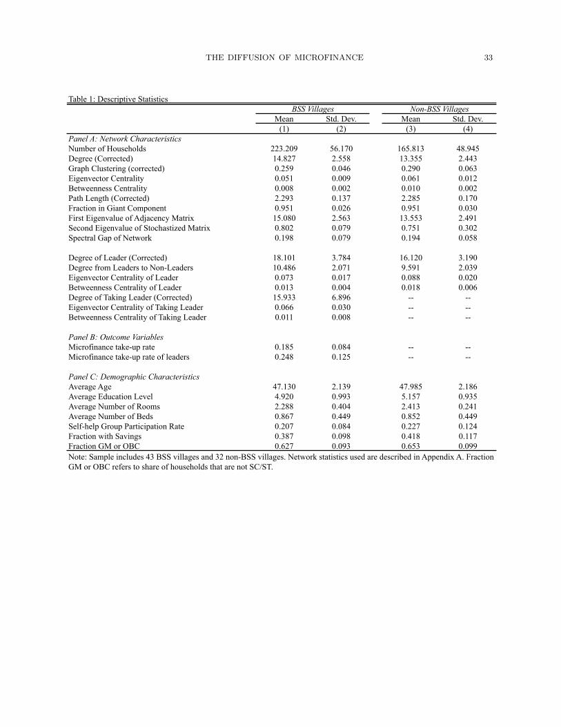
2.4. Descriptive Statistics. Table 1 provides some descriptive statistics. Villages have
an average of 223 households. The average take-up up rate for BSS is 18.5%, with a
cross-village standard deviation of 8.4%. On average, 12% of each of the households have
members designated as “leaders”. Leaders take up microfinance at a rate of 25% with
a standard deviation of 12.5% across villages.11 About 21% of households are members
of some SHG with a standard deviation of 8%. The average education is 4.92 standards
with a standard deviation of 1.01. The average fraction of “general” (GM) caste or “other
backward caste” (OBC) is 63% with substantial cross-village heterogeneity; the standard
deviation is 10%.12 About 39% have access to some form of savings with a standard
deviation of 10%. Leaders tend to be no older or younger than the population (with a p-
value of 0.415), though they do tend to have more rooms in their house (2.69 as compared
to 2.28 with a p-value of 0.00).
Turning to network characteristics, the average degree (the average number of con-
nections that each household has) is almost 15. The worlds are small, with an average
9See Jackson et al. (2011) for some distinctions between the structures of favor exchange networks andother sorts of networks in these data. Here, we work with all relationships since all involve contact thatenable word-of-mouth information dissemination.10Moreover, Chandrasekhar and Lewis (2011) apply a method of graphical reconstruction to estimatesome of the regressions from this paper and correct the bias due to sampling. Their results suggestthat our results in Table 3 underestimate the impact of leader eigenvector centrality on the microfinancetake-up rate, indicating that we are presenting a conservative result.11Take-up is measured as a percentage of non-leader households.12Thus, the remaining 37% are scheduled caste/scheduled tribe: groups that historically have beenrelatively disadvantaged.

THE DIFFUSION OF MICROFINANCE 10
network path length of 2.2 between households. Clustering rates are 26%: just over a
quarter of the time that some household i has connections to two other households j and
k, do j and k have a connection to each other.13
Eigenvector centrality is a key concept in our analysis of the importance of injection
points and is a recursively defined notion of centrality: A household’s centrality is defined
to be proportional to the sum of its neighbors’ centrality.14 While leader and non-leader
households have comparable degrees, leaders are more important in the sense of eigen-
vector centrality: their average eigenvector centrality is 0.07 (0.018), as opposed to 0.05
(0.009) for the village as a whole. At the village level, the 25th and 75th percentiles of
the average eigenvector centrality for the population are 0.0462 and 0.0609, while for the
set of leaders they are 0.065 and 0.092. There is considerable variation in the eigenvector
centrality of the leaders from village to village, a feature that we exploit below.
3. Conceptual Framework
Diffusion models may be separated into two primary categories.15 In pure contagion
models, the primary driver of diffusion is simply information or a mechanical transmission,
as in the spread of a disease, a computer virus, or awareness of an idea or rumor. In what
we call, for want of a better term, “endorsement effects models”, there are interactive
effects between individuals so that an individual’s behavior depends on that of his or her
neighbors, as in the adoption of a new technology, human capital decisions, and other
decisions with strategic complementarities. The dependency may in principle be positive
(for example, what other people did conveys a signal about the quality of the product,
as in Banerjee (1992)) or negative (for example, because when an individual’s neighbors
take up microfinance, they may share the proceeds with the individual, as in Kinnan and
Townsend (2010)).
13This is substantially higher than the fraction that would be expected in a network where links areassigned uniformly at random but with the same average degree, which in this case would be on theorder of one in fifteen. Such a significant difference between observed clustering and that expected in auniformly random network is typical of many observed social networks (e.g., see Jackson (2008)).14It corresponds to the ith entry of the eigenvector corresponding to the maximal eigenvalue of theadjacency matrix, normalized so that the entries sum to one across the vector.15See Jackson and Yariv (2010) for a recent overview of the literature and additional background.

THE DIFFUSION OF MICROFINANCE 11
Little research incorporates both aspects of diffusion and distinguishes between them.16
Because the reduced form implications of these different types of diffusion are quite sim-
ilar, without explicit modeling of information transmission and participation decisions,
it can be impossible to distinguish whether, for instance, an individual who has more
participating friends is more likely to participate because they were more likely to hear
about it or because they are influenced by the numbers of their friends who participate.
In this section, we propose simple models of the diffusion of microfinance that incor-
porate both the diffusion of information and the potential endorsement effects. We then
discuss reduced from implications of such models, specifically, concerning the potential
impacts of “injection points” (the first people who were informed about a program), and
differences in take-up in some villages compared to others. The bulk of our analysis will,
however, be a structural estimation of such models to disentangle basic information from
endorsement effects.
In addition to separating information from endorsement effects, our base model also
has another important and novel feature: distinguishing information passing by those
who take up microfinance from those who do not. Thus, the model allows for diffusion
by “non-infected nodes” and we can then estimate their role in diffusion.
3.1. The models. The models that we estimate have a common structure, illustrated in
Figures 1 to 5. They are discrete time models, described as follows:
• BSS informs the set of initial leaders.
• The leaders then decide whether or not to participate. In Figure 1, one leader has
decided to participate, and the other has not.
• In each period, households that are informed pass information to their neighbors,
with some probability. This probability may differ depending on the household’s
decision of whether or not to participate. Just as an illustration, in Figure 2,
the household that does not participate informs one link and the household that
participates informs three.
16This is not to say that both of these aspects are not understood to be important in diffusion (e.g., seeRogers and Rogers (2003), Newman (2002)), but rather that there are no systematic attempts to modelboth at the same time and disentangle them.

THE DIFFUSION OF MICROFINANCE 12
• In each period, households who were informed in the previous period decide, once
and for all, whether or not to participate, depending on their characteristics and
potentially on their neighbor’s choices as well (the endorsement effect). This is
illustrated in Figure 3.
• The model then repeats itself. In Figure 4, all the informed households pass the
information again to some of their contacts with some probability that depends
on their participation status, and in Figure 5, the newly informed nodes decide
again.
• The process repeats for a certain number of periods (which we will estimate in the
data).
Specifically, let pi denote the probability that an individual who was informed last
period decides to adopt microfinance, as a function of the individual’s characteristics and
peers.
In the baseline model, termed the “information” model, pi(α, β) is given by
(1) pi = P(participation|Xi) = Λ(α +X ′iβ),
where we allow for covariates (Xi), but not for “endorsement effects.”17
We then enrich the model to allow the decision to participate (conditional on being
informed), to depend on what others have done. We call this the “information model
with endorsement effects” (or sometimes the “endorsement model,” for short), and then
pEi (α, β, λ) refers to
(2) pEi = P(participation|Xi) = Λ(α +X ′iβ + λFi),
17Here, Λ indicates a logistic function so that
log
(pi
1− pi
)= α+X ′iβ.
THE DIFFUSION OF MICROFINANCE 13
where Fi is a fraction where the denominator is the number of i’s neighbors who informed
i and the numerator is the number of these who have participated in microfinance, and
where agents are weighed by their importance in the network.18
The other important parameters in these models are those that govern the per-period
probability that a household informs another. We let qN denote the probability that an
informed agent informs a given neighbor about microfinance in a round, conditional on
the informed agent choosing not to participate in microfinance, and qP denote the prob-
ability that an informed agent informs a given neighbor in a round about microfinance,
conditional on the agent having chosen to participate in microfinance.
We refer to the models in terms of the parameters that apply as follows:
(1) Information Model:(qN , qP , pi(α, β)
).
(2) Information Model with Endorsement Effects:(qN , qP , pEi (α, β, λ)
).
Before fitting these models, we discuss the reduced form implications of the models
at the aggregate level: what differences would we expect in the take up of microfinance
between villages based on their network characteristics?
3.2. Injection Points. A first characteristic that may differentiate the villages are the
“injection points”, or the first villagers to be informed. The idea that injections points may
matter has roots in the opinion leaders of Katz and Lazarsfeld (1955) (e.g., see Rogers
and Rogers (2003) and Valente and Davis (1999)), as well as measurements of “key”
individuals based on their influence of other’s behaviors (e.g., Ballester et al. (2006)),
and underlie some “viral marketing” strategies (e.g., see Feick and Price (1987); Aral and
Walker (Forthcoming)).
Surprisingly, there is little theory explicitly modeling the role of injection points in
information or endorsement effects models. However, it is clear that properties of the ini-
tially informed individuals could substantially impact diffusion. Regardless of the model
(information or endorsement effect), a first obvious hypothesis is that if the set of ini-
tially informed individuals in one village have a greater number of connections relative to
18In what follows, we use eigenvector centrality as a measure of network importance, and weight thefraction accordingly. In a supplementary appendix we also discuss other weightings, including degree andneutral weightings, but the eigenvector is the best-performing weighting.
THE DIFFUSION OF MICROFINANCE 14
another village, then initial information transmission could be greater, and the chance of
a sustained diffusion could be higher.19 As time goes by, and the friends of the leaders
have had time to inform their own friends, a second hypothesis is that another measure
of the centrality of the initial leaders that captures their network reach, their eigenvector
centrality, would start mattering more and more. This is in line with the ideas behind
eigenvector centrality, which measures an individual’s centrality by weighting his or her
neighbors’ centralities, instead of simply counting degree. Moreover, if there are endorse-
ment effects beyond information diffusion, the participation decisions of these leaders may
also affect participation in the village.
As described in detail below, BSS strategy of contacting the same category of people
(the “leaders”) when they first start working in a village provides village to village vari-
ation, which, we will argue, leads to plausibly exogenous variation in the degrees and
the eigenvector centrality of the first people to be informed. We take advantage of this
variation to identify the effect of the characteristics of the initial injection points on the
eventual village level take-up. We examine the extent to which take-up correlates with
the degree of the leaders, as well as their eigenvector centrality, and other measures of
their influence. In addition, as we observe take-up over time, we can also see which
characteristics of the leaders correlate with earlier versus later take-up.
3.3. Network Characteristics. While it is important to examine how the initial seeding
affects diffusion in a social network, there are other aspects of social network structure
that could also matter in diffusion. We therefore examine how take-up correlates with
other network characteristics.
In particular, in most contagion models, adding more links increases the likelihood of
non-trivial diffusion and its extent.20 For instance, Jackson and Rogers (2007) examine a
standard SIS infection model and show that if one network is more densely connected than
another in a strong sense (i.e. its degree distribution stochastically dominates the other’s),
19For example, working with a basic SIR model, the probability of the initially infected nodes’ interactionswith others would affect the probability of the spread of an infection. See Jackson (2008) for additionalbackground on the concepts discussed in this section.20See Chapter 7 in Jackson (2008) for additional discussion and theoretical background.

THE DIFFUSION OF MICROFINANCE 15
then the former network will be more susceptible to a non-trivial diffusion and have a
higher infection rate if diffusion occurs. In addition, how varied the degrees (number
of links) are across individuals in a network can affect diffusion properties, since highly
connected nodes can serve as “hubs” that play important roles in facilitating diffusion
(see Valente and Davis (1999), Pastor-Satorras and Vespignani (2000), Newman (2002),
Lopez-Pintado (2008), and Jackson and Rogers (2007)).
In addition to the distribution of degrees within a population, there are other networks
characteristics that can also affect diffusion, such as how segregated the network is. Having
a network that is strongly segregated can significantly slow information flow from one
portion of the network to another. This can be measured via the second eigenvalue of a
stochasticized adjacency matrix describing communication on the network, as shown by
Golub and Jackson (2009).
To estimate the effects of variation in these aspects of network structure on take-up, we
again take advantage of cross-village variation. However, for this analysis it is not entirely
clear the extent to which we should expect significant effects of these characteristics on
take-up. First, in much of the theory once one exceeds minimum connectivity thresholds
the extent of the diffusion is no longer as significantly impacted by network structure per
se, but by other characteristics of the nodes and their decision making.21 Second, while
there was exogenous variation in the injection points that allowed for identification and
potentially some causal inference, any variation in network structure across villages could
be endogenous and correlated with other factors influencing take-up.
Given these obstacles, we report the results of regressions of take-up on various net-
work characteristics for the sake of completeness, but then we move on to our structural
estimation, which allows us to identify and test effects that cannot be identified via a
regression-style analysis.
21Diffusion thresholds in standard contagion models are around 1 effective contact per node. This is notsimply one link per node, but at least one link through which an infection would be expected to pass ina given period. So if there is some randomness in contact through links, it is the effective contact thatmatters (e.g., see Jackson (2008)). This aspect will be picked up when we explicitly estimate informationpassing in our structural modeling, but might not turn out to be directly related to the average degreewithin a village.

THE DIFFUSION OF MICROFINANCE 16
4. Preliminary Evidence: Do Injection Points and/or Network
Structure Matter?
4.1. Injection points.
4.1.1. Identification strategy. In general, identifying the impact of the network charac-
teristics of the first people informed with a new idea (like microfinance) is difficult for
two reasons: first, even when there is data on adoption over time, most data sets do not
distinguish between information and adoption. The first people informed may not adopt,
for example. Second, information that is first received by, for example, the most popular
people in a network may also spread faster for other reasons (for example, a competent
marketing strategist may both identify the most central people in a network and inform
them first, and then also conduct an efficient generalized information campaign).
BSS methodology of spreading information about their program motivates our iden-
tification strategy to assess the causal effect of the network characteristics of the first
people informed about microfinance. When entering a village, BSS gives instructions to
its workers to contact people who fill a specific list of roles in a village (whom we have
called “leaders”): saving self-help group (SHG) leaders, pre-school (anganwadi) teachers,
and shop owners. The set of individuals they attempt to contact is fixed, and does not
vary from village to village. Upon entering a village, BSS staff identify and rely on such
individuals to disseminate information about microfinance and to help orchestrate the
first village-wide meeting.
This methodology for spreading information helps in the identification of any causal
effect of the network characteristics of the first people to be informed about the product
for two reasons. First, we know that they are the injection point for microfinance in the
village. Second, we know that they are not selected with any knowledge of their village’s
network characteristics or their position in the network, or with any consideration for the
village’s propensity to adopt microfinance.
Of course, there could still be some omitted variable bias: it could conceivably be
the case that villages where “leaders” are, say, less important or less connected are also

THE DIFFUSION OF MICROFINANCE 17
less likely to take up microfinance for other reasons. However, we show in Table 2 that
neither the eigenvector centrality nor the degree of the leaders is correlated with other
village variables. This is reassuring, as it suggests that the network characteristics of the
leader sets may be considered to be exogenous. We thus regress microfinance take-up on
the network characteristics of the “leaders” (degree, and eigenvector centrality).
Specifically, we estimate regressions of the form
(3) yr = β0 + β1 · ξLr +W ′rδ + εr
where yr is the average village level microfinance take-up, ξLr is a vector of network sta-
tistics for the leaders (we introduce, separately and together, degree and eigenvector
centrality),22 and Wr is a vector of village level controls.
Though it is likely to be endogenous, we also display specifications where we introduce
the centrality of the leaders who have become microfinance members:
(4) yr = β0 + β1 · ξLr + β2 · ξLMr +W ′rδ + εr
where ξLMr is vector of the set of leaders who became microfinance members.
We also explore whether the correlation pattern changes over time. For this investiga-
tion, we exploit data provided by BSS about participation at several points in time since
the introduction of the program (from 2/2007 to 12/2010 across 43 villages). As discussed
above, a pattern that we might expect is that the degree of leaders matters more initially
(because degree correlates with how many people they regularly interact with) while their
importance (eigenvector centrality) would matter more later, after the information has
had time to diffuse (because the people they contacted were themselves more influential).
To test this hypothesis, we run regressions of the following form:
(5) yrt = β0 + β1 · ξLr × t+ (Xr × t)′δ + αr + αt + εrt
22See the supplementary appendix for other regressions including betweenness centrality, which does notsignificantly matter.

THE DIFFUSION OF MICROFINANCE 18
where yrt is the share of microfinance take-up in village r at period t, ξLr is the average
degree and/or the average eigenvector centrality for the set of leaders and Xr is a vector
of village level controls, αr are village fixed effects, and αt are period fixed effects. The
standard errors are clustered at the village level.
As before, we also include a specification where we introduce degree and eigenvector
centrality over time.
This regression include village fixed effects, and is thus not biased by omitted village
level characteristics. The coefficient β1 will indicate whether degree (or eigenvector cen-
trality) becomes less (more) correlated with take-up over time.
4.1.2. Results. The results are presented in Tables 3 and 4. Basic cross sectional results
are presented in Table 3. The average degree of leaders is not correlated with eventual
microfinance take-up. However, their eigenvector centrality is. The coefficient of 1.6,
in column (1), implies that when the eigenvector centrality of the set of leaders is one
standard deviation larger, microfinance take-up is 2.7 percentage points (or 15%) larger.
The results are robust to introducing degree and eigenvector centrality at the same time.
They are also robust to the introduction of control variables. Interestingly, we do not find
that, conditional on the centrality of the leaders as a whole, the centrality of the leaders
who become members themselves is more strongly correlated with eventual take-up. A
potential intuition for this result is that leaders are conduits of information regardless of
their eventual participation.
Table 4 presents evidence on how the impacts of degree and eigenvector centrality of
leaders vary over time, where a period is a four-month block. In all specifications, we
find that the eigenvector centrality of the set of leaders matters significantly more over
time. The point estimate in column (1), for example, suggest that, in each period, a
one standard deviation increase in the centrality of the leader set is associated with an
increase in the take-up rate which is 0.35 percentage points greater. The point estimate of
the interaction between degree and time is always negative, although it is not significant.
As before, we find a perhaps counterintuitive result for the centrality of the the subset
of leaders who take up: if anything, it seems that their centrality matters less over time

THE DIFFUSION OF MICROFINANCE 19
(relative to that of the other leaders). This could be explained by the microfinance take-
up decisions of the leaders–it is possible that the leaders who don’t take up are more
important and busy people and therefore have more influence.
Overall, these results strongly suggest that social networks play a role in the diffusion
of microfinance and the people chosen by BSS to be the first to be informed are indeed
important in the diffusion process. However, these reduced-form results cannot shed light
on the specific form that diffusion takes in the village. The theoretical models only provide
partial guidance on what reduced form pattern should be expected. Even the result that
the centrality of the leaders who take up microfinance more does not seem to matter more
than that of the average leaders is not necessarily proof that the model of diffusion is a
pure information model. To distinguish between models, we exploit individual data and
our knowledge of the initial “injection point” (BSS leaders) to estimate structural models
of information diffusion.
4.2. Variation in Network Structure and Diffusion. Before turning to the structural
model, we next examine the correlation between village-level participation rates (measured
after about a year) on a set of variables that capture network structure including: number
of households, average degree, clustering, average path length, the first eigenvalue of the
adjacency matrix, and the second eigenvalue of the stochasticized adjacency matrix. We
include the variables both one by one and together.23
Table 5 presents the results of running regression of the form
(6) yr = W ′rβ +X ′
rδ + εr
where yr is the fraction of households joining microfinance, Wr is a vector of village-level
network covariates and Xr is a vector of village-level demographic covariates.
While there is some correlation between the network statistics and average participation
in the microfinance program when they are introduced individually (some of them counter-
intuitive; for example, average degree appears negatively correlated with take-up), no
23We present here the regression without control variables, but the results are similar when we controlfor two variables that seem to be strongly correlated with microfinance take-up, namely participation inself-help groups and caste structure.

THE DIFFUSION OF MICROFINANCE 20
variable is significant when we introduce them together. However, as discussed above, it
could be that variation in average degree is not really capturing variations across villages
in actual information passing. Also, it is important to note that the correlations are at
best suggestive: villages with particular network characteristics may also be more likely
to take up microfinance for reasons that have nothing to do with the network, leading to
downward or upward bias. There is also a strong degree of correlation between some of the
network variables (see Appendix Tables A-1 and A-2), so that they cannot be examined
independently, but, given the small number of villages, multicollinearity may obscure
relevant patterns. This may be an artifact of the lack of a well-specified functional form:
theory does not offer much guidance beyond the general prediction that there should be
a correlation between some of these network characteristics and diffusion. As we show
next, a more structured approach sheds much more light on the transmission mechanism
in the network.
5. Structural Estimation
5.1. Estimation method. As a reminder, we are seeking to estimate the following mod-
els:
(1) Information Model:(qN , qP , pi(α, β)
).
(2) Information Model with Endorsement Effects:(qN , qP , pEi (α, β, λ)
).
The formulation of these models is as was described in equations 1 and 2 and the full
algorithm of how we fit these is described in Appendix B. We begin with a non-technical
discussion of our estimation method. We use the method of simulated moments (MSM),
where we match key moments (where memp,r denotes the vector of empirical moments for
village r). We work with two sets of moments. The first set of moments exploits most of
the available variation in microfinance take-up:
(1) Share of leaders who take up microfinance (to identify β).
(2) Share of households with no neighbors taking up who take up.
(3) Share of households that are in the neighborhood of a taking leader who take up.

THE DIFFUSION OF MICROFINANCE 21
(4) Share of households that are in the neighborhood of a non-taking leader who take
up.
(5) Covariance of the fraction of households taking up with the share of their neighbors
who take up microfinance.
(6) Covariance of the fraction of household taking up with the share of second-degree
neighbors that take up microfinance.
For each set of moments, we first estimate β using take-up decision among the set of
leaders (who are known to be informed). To estimate qN , qP , and λ (or any subset of these
in the restricted models), we proceed as follows. The parameter space Θ is discretized
(henceforth we use Θ to denote the discretized parameter space) and we search over the
entire set of parameters. For each possible choice of θ ∈ Θ, we simulate the model 75
times, each time letting the diffusion process run for the number of periods from the data.
(On average, it runs 5 to 8 periods). For each simulation, the moments are calculated, and
we then take the average over the 75 runs, which gives us the vector of average simulated
moments, which we denote msim,r for village r. We then chose the set of parameters that
minimize the criterion function, namely
θ = argminθ∈Θ
(1
R
R∑r=1
msim,r(θ)−memp,r
)′(1
R
R∑r=1
msim,r(θ)−memp,r
).
To estimate the distribution of θ, we use a simple Bayesian bootstrap algorithm, for-
mally described in Appendix C. The bootstrap exploits the independence across vil-
lages. Specifically, for each grid point θ ∈ Θ, we compute the divergence for the rth
village, dr(θ) = msim,r(θ) − memp,r and interpolate values between grid points. We
bootstrap the criterion function by resampling, with replacement, from the set of 43
villages. For each bootstrap sample b = 1, ..., 1000 we estimate a weighted average,
Db(θ) = 1R
∑Rr=1 ω
br · dr(θ). Note that our objective function uses a weight of 1 for every
village. Here, the weights are drawn randomly to simulate resampling with replacement.
Then θb = argminθ∈ΘDb(θ)′Db(θ).

THE DIFFUSION OF MICROFINANCE 22
In order to compare the fit of some of the models which are not nested, but which are
estimated on the same criterion function, we study which model best fits the criterion
function determined by the same moments. We bootstrap the criterion function value,
evaluated at the estimated parameter θ, and look at the distribution of the difference
between the criterion functions of two models. The procedure is formally described in
Appendix C.
5.2. Discussion of identification. The first set of moments combined with the assump-
tion that all leaders are known injection points allow us to identify the parameters of the
model, but only under quite demanding assumptions.
The intuition behind the identification of endorsement effects and differential informa-
tion effects in our application can be clarified by a simple two by two example. Imagine,
for example, that qN = 0.10 and qP = 0.5 (these are the parameters that we estimate
below). Consider four individuals: one of them has one friend who is a leader, and this
leader takes up microfinance; the second one has one friend who is a leader but does not
take up microfinance; the third has four friends who are leaders, and all take microfinance;
the fourth has four friends who are leaders, and none of them take up microfinance. On
average, if the model runs for 6 periods (which is what we estimate as the average number
of periods), the probability that the first person is informed is 98%.24 The probability that
the second person is informed is 41%. The probability that the third person is informed
is essentially 1 and the probability that the fourth person is informed is 92%. Therefore,
in a pure information model, the difference in take-up between persons 1 and 2 would be
much larger than the difference in take-up between persons 3 and 4. However, the en-
dorsement effects for an informed person is a function of the average fraction of informed
friends who decide to take on microfinance: in an endorsement effects model, there would
be a difference between the take-up of persons 3 and 4, which we would not see in a pure
information model, even with different probabilities to inform.
This discussion clarifies a potential weakness in our identification strategy of endorse-
ment effects’ with this set of moments: we compare the behavior of different households
24This is simply (1− 0.56).

THE DIFFUSION OF MICROFINANCE 23
located at different positions in the network who both end up informed, as a function of
their neighbors’ decisions to take up microfinance, in order to estimate the endorsement
effect. However, it is possible, for example, that households who are neighbors of people
who take up are themselves more likely to need microfinance (in ways beyond our ability
to measure from all of our demographic information). We might end up attributing this
to endorsement in our estimation. For example, they may share a common activity, or
a common access to finance. Thus, the traditional pitfalls of the identification of peer
effects apply here as well.
We implement several robustness checks to address this concern.
First, an advantage of the structural approach is that the structure imposes more
specific patterns on the moments than the simple intuition that people who are closer
to people who take up microfinance should be more likely to take up themselves. To
distinguish the specific predictions from a simple prediction that people who are close
to each other should behave similarly, we compare these models to a more mechanical
“distance model”, which has no structural interpretation:
P(participation|di) = Λ(α + d(i, LP )ρ+X ′iβ).
Here d(i, LP ) is the distance of agent i to the set of participating leaders, so it is the
shortest path between i and the nearest leader who participates in microfinance.
We include this model as a (negative) benchmark: if it were to fit the data better
than our richer model, it would be worrisome, since then the fact that people closer to
participating leaders participate more may be due to omitted characteristics (those close
to participating leaders may have similar preferences, for example). To the extent that the
structural models do better in explaining the moments than a mechanical distance model,
there is some assurance that the results of the structural equation are indeed capturing
parameters of the structural model. In addition, we nest this model within our main
model to study how our findings hold.

THE DIFFUSION OF MICROFINANCE 24
Second, we use an entirely different set of moments to re-estimate the model. This set
of moments is directly inspired by the spirit of the reduced form regression we presented
in Section 4: it only exploits proximity to the sets of injection points.
This second set of moments is:
(1) Share of leaders who take up microfinance (to identify β).
(2) Covariance of take-up and minimum distance to leader.
(3) Variance of take-up among those who are at distance one from leader.
(4) Variance of take-up among those who are at distance two from leader.
Although, as we discuss below, these moments have different shortcomings, because
they are entirely different from those used in the first estimation (with the exception of
the first moment) and they make no use of the take-up decision, they are immune to
some of the potential homophily problems of the first strategy, and to the extent that the
results are similar, this provides reassurance that the results are valid.
Finally, we investigate the ability of the model to replicate time-series patterns in the
data (Table 4). Since the estimation of the structural model only exploits take-up in
the final period, the ability of the model to replicate the time series pattern (with the
eigenvector centrality of the leaders mattering increasingly over time) is a useful “out of
sample” test for the model.
5.3. Results. Table 6 presents the result of the estimation (using the first set of moments)
and Table 7 presents the result of the model selection with the quantiles of bootstrapped
values of the difference in information functions (a negative value at all quantiles repre-
sented means that model A fits the data better).
Panel A.1 presents the parameters of the information model. qN is 0.10, and qP is
0.50, and both of these are significantly different from 0. What this suggests is that in
every round informed people who are themselves participating in the program inform any
given neighbor with probability .5, and those who are not participating inform any given
neighbor with probability .1. We are able to reject equality of the two parameters: people
who take up microfinance themselves are more likely to inform their neighbors than people
who do not.

THE DIFFUSION OF MICROFINANCE 25
Panel A.2 presents estimates of the endorsement model, where the agent gives different
weights to the decision of their informed neighbors.25 There does not appear to be an extra
endorsement effect over and above the information effect: conditional on being informed,
an agent’s decision to take up microfinance is not affected by what their neighbors chose
to do themselves.
The information model where the probability that someone passes information to a
neighbor is affected by whether they are informed or not, but where there are no additional
endorsement effect is thus the structural model that fits the data the best. Moreover, as
we show in Table 7, this model provides a better fit for the key moments in the model
than a mechanical “distance to the leaders who take microfinance model”. We can reject
(at the 5% level) that the distance model fits the data better than the information model.
Finally, we can also check to see how substantial the role of non-participants is in passing
information. Even though they pass information at a much lower rate than participants,
there are many more non-participants in a village than participants. In fact, our estimates
indicate that information passing by non-participants is responsible for a third of overall
informedness and participation. We find this by comparing the model as fit above to what
would happen if only participants spread information. That is, holding all else constant,
we can then simulate the model when we set qN to 0, and see how the fraction of informed
households changes and how the take-up rate changes. We estimate that there would be a
decline of roughly one-third in overall participation, from more than 20.2 percent to 13.7
percent, and a similar decline in the fraction of informed agents, from over 81 percent
to 57 percent. Thus, not only is the level of information passing by non-participants
statistically significant (and different from that of participants), but it also appears to
play a substantial role in the spread of information passing and eventual take-up.
5.4. Robustness Checks and Alternative Specification. As we discussed, one po-
tential concern with these results is that the structural estimation approach inherits the
traditional correlated effects and endogeneity problems that plague any effort to estimate
25We present results where the weight given to a node is proportional to its eigenvector centrality, whichfit the data better than other weighting schemes in our estimations, but those models gave similar results.

THE DIFFUSION OF MICROFINANCE 26
peer effects from observational data. One reassuring aspect is that these problems tend
to bias such estimates upwards and we are not finding such effects. Nonetheless, it is
still useful to perform robustness checks as the possible biases in information parameter
estimates are less obvious. The model makes a much more specific prediction about the
diffusion of microfinance than “people close to people who take up will take up them-
selves”, so it is encouraging that it fits the data better than the mechanical “distance to
taking leader model”. But there remains a concern that the pattern we identify may be
spurious. To address this, we perform several robustness and specification checks, which
we apply to the model that is found to fit the data better, namely the pure information
model.
5.4.1. A different set of moments. Our first strategy is to estimate the model with an
entirely different set of moments. These alternative moments take advantage of the speci-
ficity of our setting, where BSS identity a specific set of “leaders” that are known to be
informed. The moments are as follows:
(1) Share of leaders who take up microfinance (to identify β).
(2) Covariance of take-up and minimum distance to leader.
(3) Variance of take-up among those who are at distance one from leader.
(4) Variance of take-up among those who are at distance two from leader.
What we are exploiting here is the difference in behavior between people who are more
or less directly connected to the leaders (and hence more or less likely to be informed).
The second moment (covariance of take-up and minimum distance to leader) is intuitive:
people closer to the leaders are more likely to be informed, and therefore should take up
more to the extent that take-up depends on information. The last two moments allow us
to separately identify qN and qP : if they are equal, the variance in take-up should increase
less between distance 1 and distance 2 than if they are different.
The identification assumption in this case is that friends of leaders are similar to other
people in the network in terms of their propensity to take up microfinance. In Appendix
D Table A-3, we investigate whether these people are different from others in the network.
We show that people who are further from leaders have fewer friends and are less central.

THE DIFFUSION OF MICROFINANCE 27
They are, however, no less likely to be part of an SHG, which is encouraging since SHG
membership could indicate an underlying demand for a microcredit product. There is no
clear pattern concerning other individual and household characteristics: people further
away from leaders have smaller homes and less education, but are more likely to have a
latrine and electricity.
To partially address this, we control for individual characteristics. We also recognize
that there could still be potential biases. But because the source of variation is completely
different than that for the first set of moments, and the source of potential biases is also
different (we worry more about the heterogeneity of people who are close to leaders,
but not about correlated effects), if the effects are the same, it will be nevertheless be
encouraging (as a form of an over-identification test), since the biases have no reason to
give us the same results. The results are presented in Panel B of Table 6. They are similar
to the first set of results: we find qN = 0.10 and qP = 0.60, and the difference between
the two remains significant.
5.4.2. A Placebo Test: Does the model predict tile roof adoption? Our second robustness
check is a placebo test. If we are really missing some unobservable correlated effects that
end up biasing our model, then they would also end up biasing the model relative to a
decision which would have the same correlated effects but would clearly not be dependent
on information passing. Thus, instead of using microfinance participation as the predicted
variable, we use a “placebo” outcome: does a household have a tiled roof? The share of
households who have such a roof is 32%, and having one may be correlated with wealth,
which is probably correlated among people who are neighbors in the network, and so the
potential biases will be present. On the other hand, there should no role for information
passing when we fit our model. Thus, if our model technique is biased, then it would
appear as if there is a critical role for information passing when there is not.
The model is estimated with the same set of moments as the main model by simply
replacing microfinance participation with type of roof. The results, presented in Panel C
of Table 6, are interesting: we find a much greater estimated qN and qP (0.90 and 0.80
respectively, with qN actually greater than qP , although the difference is not statistically

THE DIFFUSION OF MICROFINANCE 28
significant). Overall, these estimates are different from the ones we obtain with microfi-
nance, suggesting that the results may not be driven by selection bias. It is important to
note that the estimated parameters in the model must be high in order to permit deci-
sions to not be affected by information. If the parameters were low, then nobody would
be informed and nobody could choose to have a tiled roof. Thus, if there is no effect, the
parameters should be close to 1 and no different from each other, exactly as we find.
5.4.3. Controlling for social distance to leaders who took up microfinance. Our third check
is to control for the most direct source of possible bias in our main estimate, which is
that people who are close to leaders who chose to take up microfinance may themselves
have a greater need for microfinance. We saw that the mechanical “distance to leaders
who take up” model fits the data less well than our information model. However, can we
go further and add a linear control for the social distance to leaders who chose to take
up microfinance in our main MSM simulation. This nested specification ensures that our
estimation relies on the specific functional form implied by the model, rather than by
correlation in behavior.
The result of introducing the nearest distance to a leader who took up microfinance in
the information model is presented in Panel D of Table 6. Both estimates are higher than
before, particularly qP , which is 0.90. The difference between the two stays significant,
however.
5.5. How well does the model predict the aggregate patterns? Finally, to provide
a test of the fit of the model, we attempt to replicate the basic cross-village patterns that
we presented in the beginning of the paper. We do this for the information model, without
enforcement, and set qN = 0.1 and qP = 0.5. To do so, we simulate the information model
in each of our networks, construct the basic statistics that we had constructed in the
real data for the simulated data, and run exactly the same regressions. The basic cross-
sectional pattern are not interesting to replicate, since village level take up of microfinance
is one of the moment we match. However, we make no use of the time-series structure of
the data in the structural estimation. Thus, the ability of the simulated data over time

THE DIFFUSION OF MICROFINANCE 29
to match the pattern observed in the data over time is a useful cross-validation of our
structural model.
Table 8 presents results regarding whether the model is able to replicate time series
patterns found in the data, where the average eigenvector centrality of the leaders was
found to matter increasingly over time. Consistent with the real data, we find, in the
simulated data that the average eigenvector centrality of the leaders matters increasingly
over time. Although, the point estimate in the simulated data is smaller, if we restrict
the regression to time periods 2 and onward then the model also produces quantitatively
similar coefficients. Therefore, the model better replicates later periods of the diffusion
process, only partially replicating first period dynamics.26
6. Conclusion
Taking advantage of arguably exogenous variation in initially informed individuals
across villages induced by BSS strategy, we show that the eigenvector centralities of ini-
tially informed individuals are significant determinants of the eventual participation rate
in a village; in contrast, other variations in social network characteristics across villages
are relatively insignificant determinants of diffusion.
Motivated by these patterns, we have used the micro-data to estimate a structural model
of the diffusion of information in the social network. While this estimation requires some
stronger identification assumptions, it allows us to distinguish between different models
of information transmission. We find that the data appears to be well-characterized
by a model where participants pass information with much higher likelihood than non-
participants, but nonetheless that both forms of information passing are important. The
estimation also suggests that once informed, an individual’s decision is not significantly
affected by the participation of her acquaintances, suggesting no extra endorsement effects
over and above information transmission.
26As periods in the model are rounds of communication, they may not correspond to either calendar timeor rounds of sign-ups, and so we might expect better matching of long-run than short run dynamics.

THE DIFFUSION OF MICROFINANCE 30
The information model fits the data better than a mechanical “distance” model (where
adoption is a function of distance to a participating leader), and does a good job repli-
cating the aggregate cross sectional pattern in the data (including the lack of prediction
concerning any of the social network characteristics and the eventual participation). The
results hold up under several robustness checks: in particular, when we re-estimate the
model using an entirely different set of moments, and when we re-estimate the model
with a different participation variable where we know the information effect should not
be present.
Our findings not only shed light on microfinance, but also suggest that further research
is important. First, the fact that the initial injection points are a major predictor of
diffusion in our setting suggests that more attention should be paid to initial conditions
in both the theoretical and empirical analysis of diffusion. Second, the fact that we
find differences in the role of pure information versus endorsement effects in this setting
suggests that it will be useful to develop richer models of peer effects and diffusion that
further disentangle the various roles that interactions can play, and to investigate this
dichotomy across a wider range of applications. Finally, the role of non-participants in
diffusion is also noteworthy and deserving of further attention in other settings.
References
Aral, S., L. Muchnik, and A. Sundararajan (2009): “Distinguishing Influence
Based Contagions from Homophily Driven Diffusion in Dynamic Networkss,” Proceed-
ings of the National Academy of Science.
Aral, S. and D. Walker (Forthcoming): “Creating social contagion through viral
product design: A randomized trial of peer influence in networks,” Management Sci-
ence.
Ballester, C., A. Calvo-Armengol, and Y. Zenou (2006): “Who’s who in net-
works. wanted: the key player,” Econometrica, 74, 1403–1417.
Banerjee, A. V. (1992): “A Simple Model of Herd Behavior,” Quarterly Journal of
Economics, 107, 797–817.

THE DIFFUSION OF MICROFINANCE 31
Breza, E., A. G. Chandrasekhar, and H. Larreguy (2011): “Punishment on
Networks: Evidence from a lab experiment in the field,” MIT Working Paper.
Chandrasekhar, A. G., C. Kinnan, and H. Larreguy (2011a): “Informal Insur-
ance, Social Networks, and Savings Access: Evidence from a lab experiment in the
field,” MIT Working Paper.
——— (2011b): “Information, Savings, and Informal Insurance: Evidence from a lab
experiment in the field,” MIT Working Paper.
Chandrasekhar, A. G. and R. Lewis (2011): “Econometrics of Sampled Networks,”
MIT working paper.
Coleman, J., E. Katz, and H. Menzel (1966): Medical Innovation: A Diffusion
Study, Indianapolis: Bobbs-Merrill.
Feick, L. and L. Price (1987): “The market maven: A diffuser of marketplace infor-
mation,” The Journal of Marketing, 83–97.
Golub, B. and M. O. Jackson (2009): “How Homophily Affects the Speed of Learning
and Best Response Dynamics,” SSRN Paper 1786207.
Jackson, M. O. (2008): Social and economic networks, Princeton University Press.
Jackson, M. O., T. Barraquer, and X. Tan (2011): “Social Capital and Social
Quilts: Network Patterns of Favor Exchange,” American Economic Review, forthcom-
ing.
Jackson, M. O. and B. Rogers (2007): “Relating network structure to diffusion
properties through stochastic dominance,” The BE Journal of Theoretical Economics,
7, 1–13.
Jackson, M. O. and L. Yariv (2010): “Diffusion, strategic interaction, and social
structure,” in Handbook of Social Economics, edited by J. Benhabib, A. Bisin and M.
Jackson.
Katz, E. and P. Lazarsfeld (1955): Personal Influence: The Part Played by People
in the Flow of Mass Communication, New York: Free Press.
Kinnan, C. and R. M. Townsend (2010): “Kinship and Financial Networks, Formal
Financial Access and Risk Reduction,” unpublished manuscript.
THE DIFFUSION OF MICROFINANCE 32
Lazarsfeld, P., B. Berelson, and G. Gaudet (1944): The people’s choice: How
the voter makes up his mind in a presidential campaign, New York: Duell, Sloan and
Pearce.
Lopez-Pintado, D. (2008): “Diffusion in complex social networks,” Games and Eco-
nomic Behavior, 62, 573–590.
Newman, M. E. J. (2002): “Spread of epidemic disease on networks,” Physical Review
E, 66, 016128(11).
Pastor-Satorras, R. and A. Vespignani (2000): “Epidemic Spreading in Scale-Free
Networks,” Physical Review Letters, 86, 3200–3203.
Rogers, E. and E. Rogers (2003): Diffusion of Innovations, fifth edition, New York:
Free Press.
Ryan, B. and N. C. Gross (1943): “The diffusion of hybrid seed corn in two Iowa
communities,” Rural Sociology, 8, 15–24.
Valente, T. W. and R. L. Davis (1999): “Accelerating the Diffusion of Innovations
Using Opinion Leaders,” The Annals of the American Academy of Political and Social
Science, 566, 55–67.
THE DIFFUSION OF MICROFINANCE 33
Table 1: Descriptive Statistics
Mean Std. Dev. Mean Std. Dev.(1) (2) (3) (4)
Panel A: Network CharacteristicsNumber of Households 223.209 56.170 165.813 48.945Degree (Corrected) 14.827 2.558 13.355 2.443Graph Clustering (corrected) 0.259 0.046 0.290 0.063Eigenvector Centrality 0.051 0.009 0.061 0.012Betweenness Centrality 0.008 0.002 0.010 0.002Path Length (Corrected) 2.293 0.137 2.285 0.170Fraction in Giant Component 0.951 0.026 0.951 0.030First Eigenvalue of Adjacency Matrix 15.080 2.563 13.553 2.491Second Eigenvalue of Stochastized Matrix 0.802 0.079 0.751 0.302Spectral Gap of Network 0.198 0.079 0.194 0.058
Degree of Leader (Corrected) 18.101 3.784 16.120 3.190Degree from Leaders to Non-Leaders 10.486 2.071 9.591 2.039Eigenvector Centrality of Leader 0.073 0.017 0.088 0.020Betweenness Centrality of Leader 0.013 0.004 0.018 0.006Degree of Taking Leader (Corrected) 15.933 6.896 -- --Eigenvector Centrality of Taking Leader 0.066 0.030 -- --Betweenness Centrality of Taking Leader 0.011 0.008 -- --
Panel B: Outcome VariablesMicrofinance take-up rate 0.185 0.084 -- --Microfinance take-up rate of leaders 0.248 0.125 -- --
Panel C: Demographic CharacteristicsAverage Age 47.130 2.139 47.985 2.186Average Education Level 4.920 0.993 5.157 0.935Average Number of Rooms 2.288 0.404 2.413 0.241Average Number of Beds 0.867 0.449 0.852 0.449Self-help Group Participation Rate 0.207 0.084 0.227 0.124Fraction with Savings 0.387 0.098 0.418 0.117Fraction GM or OBC 0.627 0.093 0.653 0.099
BSS Villages Non-BSS Villages
Note: Sample includes 43 BSS villages and 32 non-BSS villages. Network statistics used are described in Appendix A. Fraction GM or OBC refers to share of households that are not SC/ST.
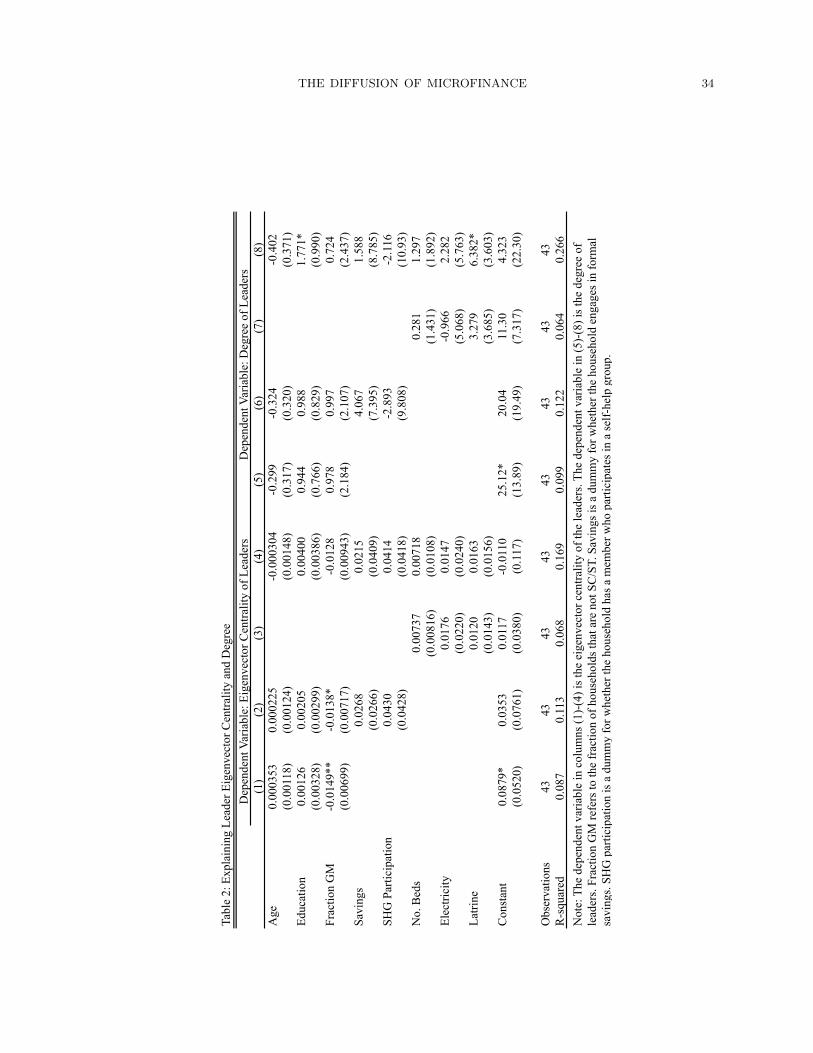
THE DIFFUSION OF MICROFINANCE 34
Tabl
e 2:
Exp
lain
ing
Lead
er E
igen
vect
or C
entra
lity
and
Deg
ree
(1)
(2)
(3)
(4)
(5)
(6)
(7)
(8)
Age
0.00
0353
0.00
0225
-0.0
0030
4-0
.299
-0.3
24-0
.402
(0.0
0118
)(0
.001
24)
(0.0
0148
)(0
.317
)(0
.320
)(0
.371
)Ed
ucat
ion
0.00
126
0.00
205
0.00
400
0.94
40.
988
1.77
1*(0
.003
28)
(0.0
0299
)(0
.003
86)
(0.7
66)
(0.8
29)
(0.9
90)
Frac
tion
GM
-0.0
149*
*-0
.013
8*-0
.012
80.
978
0.99
70.
724
(0.0
0699
)(0
.007
17)
(0.0
0943
)(2
.184
)(2
.107
)(2
.437
)Sa
ving
s0.
0268
0.02
154.
067
1.58
8(0
.026
6)(0
.040
9)(7
.395
)(8
.785
)SH
G P
artic
ipat
ion
0.04
300.
0414
-2.8
93-2
.116
(0.0
428)
(0.0
418)
(9.8
08)
(10.
93)
No.
Bed
s0.
0073
70.
0071
80.
281
1.29
7(0
.008
16)
(0.0
108)
(1.4
31)
(1.8
92)
Elec
trici
ty0.
0176
0.01
47-0
.966
2.28
2(0
.022
0)(0
.024
0)(5
.068
)(5
.763
)La
trine
0.01
200.
0163
3.27
96.
382*
(0.0
143)
(0.0
156)
(3.6
85)
(3.6
03)
Con
stan
t0.
0879
*0.
0353
0.01
17-0
.011
025
.12*
20.0
411
.30
4.32
3(0
.052
0)(0
.076
1)(0
.038
0)(0
.117
)(1
3.89
)(1
9.49
)(7
.317
)(2
2.30
)
Obs
erva
tions
4343
4343
4343
4343
R-s
quar
ed0.
087
0.11
30.
068
0.16
90.
099
0.12
20.
064
0.26
6N
ote:
The
dep
ende
nt v
aria
ble
in c
olum
ns (1
)-(4
) is t
he e
igen
vect
or c
entra
lity
of th
e le
ader
s. Th
e de
pend
ent v
aria
ble
in (5
)-(8
) is t
he d
egre
e of
le
ader
s. Fr
actio
n G
M re
fers
to th
e fr
actio
n of
hou
seho
lds t
hat a
re n
ot S
C/S
T. S
avin
gs is
a d
umm
y fo
r whe
ther
the
hous
ehol
d en
gage
s in
form
al
savi
ngs.
SHG
par
ticip
atio
n is
a d
umm
y fo
r whe
ther
the
hous
ehol
d ha
s a m
embe
r who
par
ticip
ates
in a
self-
help
gro
up.
Dep
ende
nt V
aria
ble:
Eig
enve
ctor
Cen
tralit
y of
Lea
ders
Dep
ende
nt V
aria
ble:
Deg
ree
of L
eade
rs

THE DIFFUSION OF MICROFINANCE 35
Tabl
e 3:
Lea
ders
/Inje
ctio
n po
ints
Take
-up
Rat
eTa
ke-u
p R
ate
Take
-up
Rat
eTa
ke-u
p R
ate
Take
-up
Rat
eTa
ke-u
p R
ate
(1)
(2)
(3)
(4)
(5)
(6)
1.63
4*1.
934*
*1.
843
1.25
4*1.
332*
(0.9
04)
(0.9
67)
(1.1
01)
(0.7
35)
(0.7
82)
Num
ber o
f Hou
seho
lds
-0.0
0038
2-0
.000
704*
**-0
.000
270
-0.0
0027
3-0
.000
305
-0.0
0029
9(0
.000
247)
(0.0
0018
8)(0
.000
270)
(0.0
0028
0)(0
.000
216)
(0.0
0022
6)D
egre
e of
Lea
ders
-0.0
0111
-0.0
0324
-0.0
0287
(0.0
0231
)(0
.002
59)
(0.0
0276
)Fr
actio
n of
Tak
ing
Lead
ers
0.32
3***
0.31
7***
(0.1
01)
(0.1
05)
-0.1
75-0
.253
(0.4
28)
(0.4
27)
Savi
ngs
-0.0
568
-0.0
523
(0.0
940)
(0.0
854)
Frac
tion
GM
-0.0
151
-0.0
0792
(0.0
363)
(0.0
302)
Con
stan
t0.
150
0.36
2***
0.16
20.
292
0.09
240.
0924
(0.1
12)
(0.0
573)
(0.1
06)
(0.2
02)
(0.0
915)
(0.1
86)
Obs
erva
tions
4343
4343
4343
R-s
quar
ed0.
293
0.23
50.
311
0.31
90.
502
0.50
2
Eige
nvec
tor C
entra
lity
of L
eade
rs
Eige
nvec
tor C
entra
lity
of T
akin
g Le
ader
s
Not
e: D
epen
dent
var
iabl
e is
the
mic
rofin
ance
par
ticip
atio
n ra
te o
f non
-lead
er h
ouse
hold
s and
repo
rt he
tero
sked
astic
robu
st
stan
dard
err
ors.

THE DIFFUSION OF MICROFINANCE 36
Table 4: Leader Characteristics that Matter Over TimeTake-Up Rate Take-Up Rate
(1) (2)0.3511*** 0.3491**
(0.128) (0.1635)Degree of Leaders -0.00075 -0.00063
(0.00082) (0.00088)Number of Households -0.000016
(0.00003)Savings 0.0082
(0.0109)Fraction GM 0.0049
(0.0031)
Observations 239 239R-squared 0.943 0.944
Eigenvector Centrality of Leaders
Note: The dependent variable is the microfinance take-up rate in a village in a time period. Every covariate is interacted with time. Regressions include village fixed effects and time fixed effects. Standard errors are clustered at the village level.

THE DIFFUSION OF MICROFINANCE 37
Tabl
e 5:
Net
wor
k C
hara
cter
istic
s and
Par
ticip
atio
nTa
ke-u
p R
ate
Take
-up
Rat
eTa
ke-u
p R
ate
Take
-up
Rat
eTa
ke-u
p R
ate
Take
-up
Rat
eTa
ke-u
p R
ate
(1)
(2)
(3)
(4)
(5)
(6)
(7)
Num
ber o
f Hou
seho
lds
-0.0
0072
1***
-0.0
0027
8(0
.000
185)
(0.0
0073
7)D
egre
e-0
.007
79*
-0.0
231
(0.0
0443
)(0
.026
4)C
lust
erin
g C
oeffi
cien
t0.
0693
0.34
8(0
.304
)(0
.684
)Pa
th L
engt
h-0
.100
-0.2
19(0
.084
8)(0
.364
)Fi
rst E
igen
valu
e of
Adj
acen
cy M
atrix
-0.0
0851
*0.
0071
8(0
.004
55)
(0.0
205)
Seco
nd E
igen
valu
e of
Sto
chas
tized
Mat
rix-0
.156
-0.0
179
(0.1
88)
(0.3
04)
Con
stan
t0.
346*
**0.
300*
**0.
167*
*0.
414*
*0.
313*
**0.
310*
*0.
906
(0.0
469)
(0.0
712)
(0.0
785)
(0.1
93)
(0.0
737)
(0.1
52)
(0.8
39)
Obs
erva
tions
4343
4343
4343
43R
-squ
ared
0.23
20.
056
0.00
10.
027
0.06
70.
021
0.26
7N
ote:
Dep
ende
nt v
aria
ble
is th
e m
icro
finan
ce p
artic
ipat
ion
rate
of n
on-le
ader
hou
seho
lds.
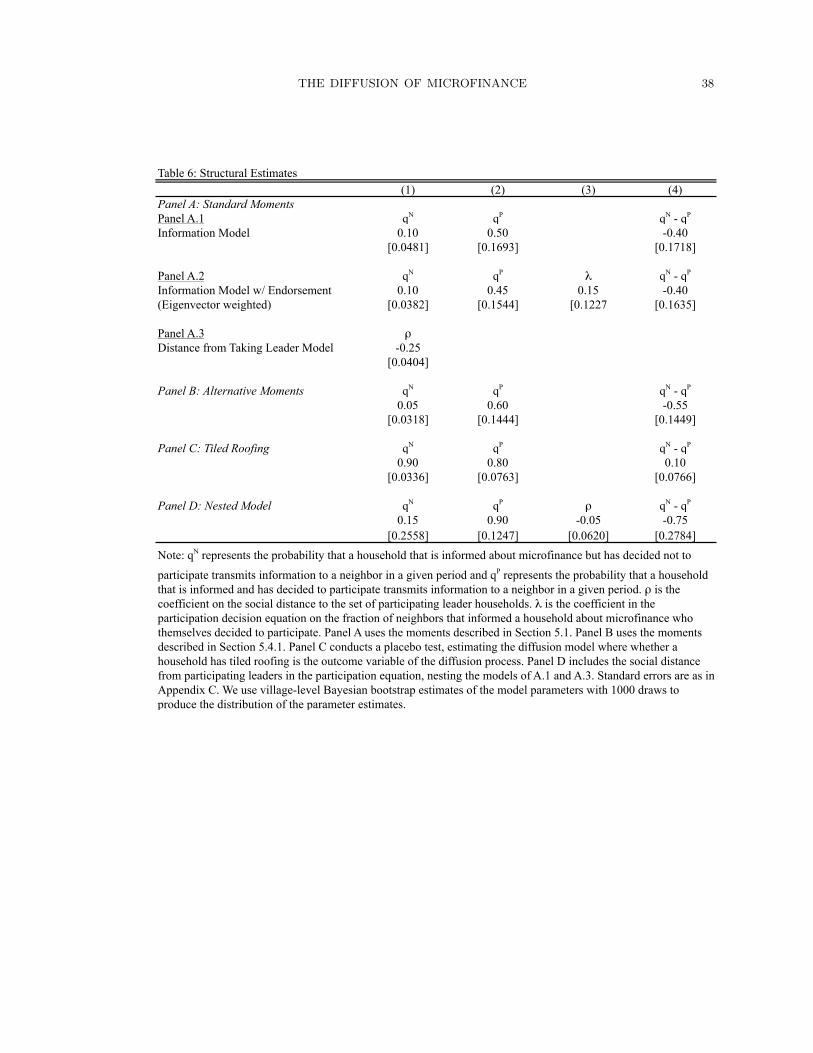
THE DIFFUSION OF MICROFINANCE 38
Table 6: Structural Estimates(1) (2) (3) (4)
Panel A: Standard MomentsPanel A.1 qN qP qN - qP
Information Model 0.10 0.50 -0.40[0.0481] [0.1693] [0.1718]
Panel A.2 qN qP λ qN - qP
Information Model w/ Endorsement 0.10 0.45 0.15 -0.40(Eigenvector weighted) [0.0382] [0.1544] [0.1227 [0.1635]
Panel A.3 ρDistance from Taking Leader Model -0.25
[0.0404]
Panel B: Alternative Moments qN qP qN - qP
0.05 0.60 -0.55[0.0318] [0.1444] [0.1449]
Panel C: Tiled Roofing qN qP qN - qP
0.90 0.80 0.10[0.0336] [0.0763] [0.0766]
Panel D: Nested Model qN qP ρ qN - qP
0.15 0.90 -0.05 -0.75[0.2558] [0.1247] [0.0620] [0.2784]
Note: qN represents the probability that a household that is informed about microfinance but has decided not to
participate transmits information to a neighbor in a given period and qP represents the probability that a household that is informed and has decided to participate transmits information to a neighbor in a given period. ρ is the coefficient on the social distance to the set of participating leader households. λ is the coefficient in the participation decision equation on the fraction of neighbors that informed a household about microfinance who themselves decided to participate. Panel A uses the moments described in Section 5.1. Panel B uses the moments described in Section 5.4.1. Panel C conducts a placebo test, estimating the diffusion model where whether a household has tiled roofing is the outcome variable of the diffusion process. Panel D includes the social distance from participating leaders in the participation equation, nesting the models of A.1 and A.3. Standard errors are as in Appendix C. We use village-level Bayesian bootstrap estimates of the model parameters with 1000 draws to produce the distribution of the parameter estimates.

THE DIFFUSION OF MICROFINANCE 39
Table 7: Model Selection5th Percentile Median 95th Percentile
(1) (2) (3)Information Model vs Distance Model-0.058 -0.037 -0.004Note: The test statistic for Model A vs Model B is 421/2(Criterion

THE DIFFUSION OF MICROFINANCE 40
Table 8: Leader Characteristics that Matter Over TimeSimulated Data Empirical Data
Take-Up Rate Take-Up Rate Take-Up Rate Take-Up Rate(1) (2) (3) (4)
0.1069** 0.0781 0.1052* 0.1148*(0.0471) (0.0640) (0.1635) (0.0593)
Degree of Leaders 0.00048** 0.00058 0.00014 0.00016(0.00022) (0.00018) (0.000298) (0.00042)
Number of Households 0.000003(0.000018)
Savings 0.00196(0.0060)
Fraction GM -0.0064(0.0015)
Observations 239 239 196 196R-squared 0.983 0.986 0.983 0.977
Eigenvector Centrality of Leaders
Note: The dependent variable is the microfinance take-up rate in a village in a time period. Every covariate is interacted with time. Regressions include village fixed effects and time fixed effects. Standard errors are clustered at the village level. Columns (3) and (4) restricts the sample to time periods t > 1.
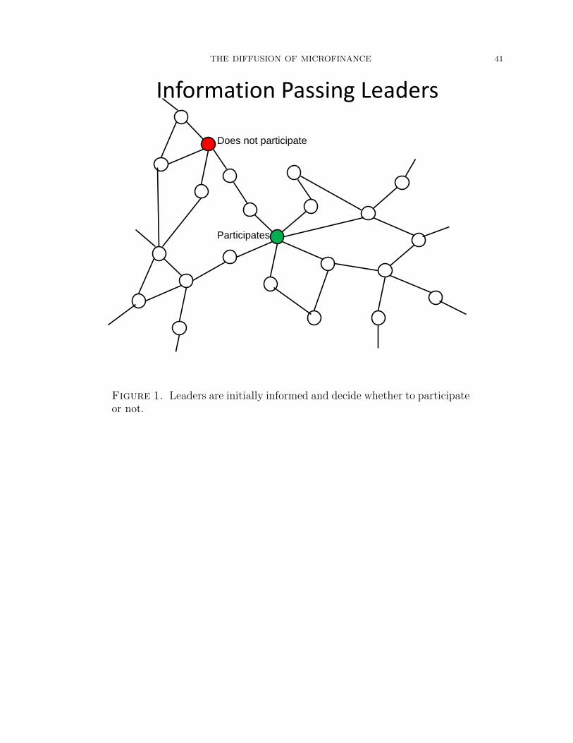
THE DIFFUSION OF MICROFINANCE 41
Information Passing Leaders
Does not participate
Participates
Figure 1. Leaders are initially informed and decide whether to participateor not.

THE DIFFUSION OF MICROFINANCE 42
Passing: Different Probabilities
Figure 2. Nodes that participate have a higher probability of passing oninformation.
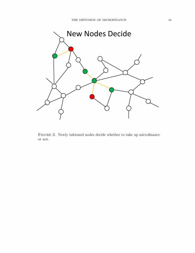
THE DIFFUSION OF MICROFINANCE 43
New Nodes Decide
Figure 3. Newly informed nodes decide whether to take up microfinanceor not.

THE DIFFUSION OF MICROFINANCE 44
Pass Again
Figure 4. Informed nodes pass on information again.

THE DIFFUSION OF MICROFINANCE 45
New Decisions, etc.
Figure 5. New decisions are made by the newly informed nodes.

THE DIFFUSION OF MICROFINANCE 46
Appendix A. Glossary of network terminology
In this section, we provide brief background definitions of some terms and variables
with respect to how they are measured in our data.27
• Degree: the number of links that a household has.
– This is a measure of how well-connected a node is in a graph.
• Clustering coefficient: the fraction of pairs of a household’s neighbors who are
neighbors of each other.
– This is a measure of how interwoven a household’s neighborhood is.
• Eigenvector centrality: a recursively defined notion of importance. A household’s
centrality is defined to be proportional to the sum of its neighbors’ centralities.
It corresponds to the ith entry of the eigenvector corresponding to the maximal
eigenvalue of the adjacency matrix.
– This is a measure of how important a node is in the sense of information flow.
• Average path length: the mean length of the shortest path between any two
households in the village.
– Shorter average path length means information has to travel less (on average)
to get from household i to household j.
• First eigenvalue: the maximum eigenvalue of the adjacency matrix representing
the network.
– This is a measure of how diffusive the network is. A higher first eigenvalue
implies that information is generally more transmitted.
• Fraction of nodes in the giant component: the share of nodes in the graph that
are in the largest connected component.
– Typically, realistic graphs have a giant component with almost all nodes in it.
Thus, the measure should be approaching one. For a network that is sampled,
this number can be significantly lower. In particular, networks which were
tenuously or sparsely connected to begin with may “shatter” under sampling
and therefore the giant component may no longer be giant after sampling. In
27Detailed descriptions can be found in Jackson (2008).

THE DIFFUSION OF MICROFINANCE 47
turn, it becomes a useful measure of how interwoven the underlying network
is.
• Second eigenvalue of the stochastized adjacency matrix: the stochastized adja-
cency matrix is defined by person i putting 1/di weight on each of her di-neighbors
and 0 weight on the rest of the individuals in the network. The second eigenvalue
is the second largest eigenvalue (in magnitude) of this matrix. The largest is
mechanically one.
– It captures a communication flow in a network. It provides bounds on the
rate of convergence of beliefs in some models (e.g., see Golub and Jackson
(2009)). Lower second eigenvalue means information convergence approaches
faster; that is, the network has a lower consensus time.

THE DIFFUSION OF MICROFINANCE 48
Appendix B. Model structure
We formally describe the model in this section. The model is simulated in discrete time
periods t ∈ N. At each point in time, a node (household) has two states that we track:
• node i’s information status: sIit ∈ {0, 1}, with 0 indicating uninformed and 1
indicating informed,28
• node i’s participation status: mit ∈ {0, 1}. Note that if mit = 1 then sit = 1 as
one cannot participate without being informed.
Let It be the set of newly informed nodes at time t.29 Define I t be the historical stock of
those informed.
The Basic Algorithm
(1) t=0
(a) At the beginning of the period, the initial set of nodes (leaders) are informed.
si0 = 1 ∀i ∈ L and si0 = 0 if i /∈ L, where L = {i ∈ N : i is a leader}.
(b) Next, those newly informed agents decide whether or not to participate: mi0
are distributed as Bernoulli with pi(α, β) or pEi (α, β, λ), for each i ∈ I1. In
the case of pEi , for the initial period Fi = 0.
(c) Next, each i ∈ I0 transmits to j ∈ Ni with probability mi1qP + (1−mi1) qN .
This is independent across i and j. Let I1 be the set of j’s informed via
this process who were not members of I0, and let I(j) be the set of i’s who
informed j.
(2) Iteration at time t:
(a) The newly informed agents are now It.
(b) Those newly informed agents decide whether or not to participate: mit are
distributed as Bernoulli with pi(α, β) or pEi (α, β, λ), for each i ∈ It. In the
case of pEi , for the initial period Fi = |{j|j ∈ I(i, t),mjt = 1}|/|I(i, t)| where
I(i, t) is the set of i’s who informed j.
28So, note that si,t+1 ≥ sit for all t.29That is It = {i : sit = 1, sit−1 = 0}.

THE DIFFUSION OF MICROFINANCE 49
(c) Next, for all nodes i ∈ I t each i transmits to j ∈ Ni with probability mitqP +
(1−mit) qN . This is independent across i. Let It+1 be the set of j’s informed
via this process who are not in I t, let I(j, t+1) be the set of i’s who informed
j, and the process repeats.
Appendix C. Structural estimation
Bootstrap Algorithm Let Θ be the parameter space and Λ a grid on Θ. Put ψ(·)
as the moment function and let zr = (yr, xr) denote the empirical data with a vector of
microfinance take-up decisions, yr, and covariates xr, including leadership status and other
covariates included in the model, for village r. Define memp,r := ψ(zr) as the empirical
moment for village r and msim,r(s, θ) := ψ(zsr(θ)) = ψ(ysr(θ), xr) as the sth simulated
moment for village r at parameter value θ. Also, put B as the number of bootstraps and
S as the number of simulations used to construct the simulated moment.
(1) Pick lattice Λ ⊂ Θ.
(2) For λ ∈ Λ on the grid:
(a) For each village r ∈ [R], compute
d(r, λ) :=1
S
∑s∈[S]
msim,r(s, θ)−memp,r.
(b) For each b ∈ [B], compute
D(b) :=1
R
∑r∈[R]
ωbr · d(r, λ)
where ωbr := ebr/er with ebr iid exp(1) random variables and er := 1R
∑ebr.
(c) Find λ?b = arg minQ?b(λ), with
Q?b (λ) := ‖D(b)‖`2,R .
(3) Obtain {λ?b}b∈B.
(4) For conservative inference, consider the 1 − α/2 and α/2 quantiles of the λ?bj
marginal empirical distribution.

THE DIFFUSION OF MICROFINANCE 50
Specifically, we consider for the information model Θ = [0, 1]2, Λ = [0.05 : 0.05 : 0.95] ×
[0.05 : 0.05 : 0.95], B = 1000, S = 75; for the endorser model Θ = [0, 1]2 × R, Λ = [0.05 :
0.05 : 0.95]2 × [−5 : 0.05 : 1], B = 1000, S = 75.
Appendix D. Misc. Tables
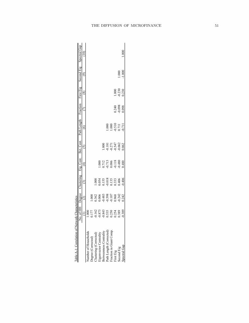
THE DIFFUSION OF MICROFINANCE 51
Tabl
e A-1
: Cor
rela
tion
of N
etw
ork
Cha
ract
eris
tics
No.
of H
HD
egre
eC
lust
erin
gEi
g. C
ent.
Bet
. Cen
t.Pa
th L
engt
hFr
actio
nFi
rst E
igSe
cond
Eig
Spec
tral G
ap(1
)(2
)(3
)(4
)(5
)(6
)(7
)(8
)(9
)(1
0)N
umbe
r of H
ouse
hold
s1.
000
Deg
ree
(Cor
rect
ed)
0.17
71.
000
Clu
ster
ing
(Cor
rect
ed)
-0.1
620.
362
1.00
0Ei
genv
ecto
r Cen
tralit
y-0
.873
0.00
60.
054
1.00
0B
etw
eenn
ess C
entra
lity
-0.8
43-0
.483
0.15
50.
712
1.00
0Pa
th L
engt
h (C
orre
cted
)0.
535
-0.5
98-0
.018
-0.7
13-0
.181
1.00
0Fr
actio
n in
Gia
nt C
omp.
0.25
0-0
.107
0.13
50.
086
-0.2
711.
000
Firs
t Eig
0.25
40.
968
0.33
3-0
.118
-0.5
47-0
.510
0.24
01.
000
Seco
nd E
ig0.
389
-0.2
420.
406
-0.4
80-0
.062
0.71
1-0
.098
-0.2
301.
000
Spec
tral G
ap-0
.389
0.24
2-0
.406
0.48
00.
062
-0.7
110.
098
0.23
0-1
.000
1.00
0
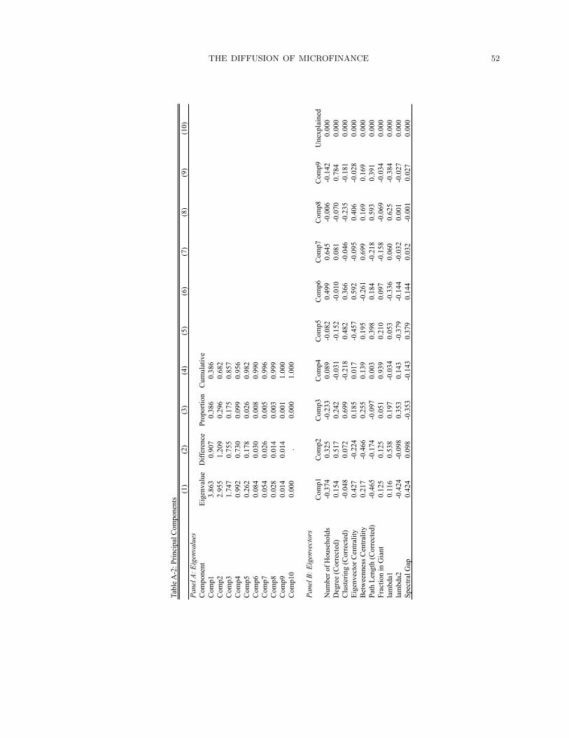
THE DIFFUSION OF MICROFINANCE 52
Tabl
e A-2
: Prin
cipa
l Com
pone
nts
(1)
(2)
(3)
(4)
(5)
(6)
(7)
(8)
(9)
(10)
Pane
l A: E
igen
valu
esC
ompo
nent
Eige
nval
ueD
iffer
ence
Prop
ortio
nC
umul
ativ
eC
omp1
3.86
30.
907
0.38
60.
386
Com
p22.
955
1.20
90.
296
0.68
2C
omp3
1.74
70.
755
0.17
50.
857
Com
p40.
992
0.73
00.
099
0.95
6C
omp5
0.26
20.
178
0.02
60.
982
Com
p60.
084
0.03
00.
008
0.99
0C
omp7
0.05
40.
026
0.00
50.
996
Com
p80.
028
0.01
40.
003
0.99
9C
omp9
0.01
40.
014
0.00
11.
000
Com
p10
0.00
0.
0.00
01.
000
Pane
l B: E
igen
vect
ors
Com
p1C
omp2
Com
p3C
omp4
Com
p5C
omp6
Com
p7C
omp8
Com
p9U
nexp
lain
edN
umbe
r of H
ouse
hold
s-0
.374
0.32
5-0
.233
0.08
9-0
.082
0.49
90.
645
-0.0
06-0
.142
0.00
0D
egre
e (C
orre
cted
)0.
154
0.51
70.
242
-0.0
31-0
.152
-0.0
100.
081
-0.0
700.
784
0.00
0C
lust
erin
g (C
orre
cted
)-0
.048
0.07
20.
699
-0.2
180.
482
0.36
6-0
.046
-0.2
35-0
.181
0.00
0Ei
genv
ecto
r Cen
tralit
y0.
427
-0.2
240.
185
0.01
7-0
.457
0.59
2-0
.095
0.40
6-0
.028
0.00
0B
etw
eenn
ess C
entra
lity
0.21
7-0
.466
0.25
50.
139
0.19
5-0
.261
0.69
90.
169
0.16
90.
000
Path
Len
gth
(Cor
rect
ed)
-0.4
65-0
.174
-0.0
970.
003
0.39
80.
184
-0.2
180.
593
0.39
10.
000
Frac
tion
in G
iant
0.12
50.
125
0.05
10.
939
0.21
00.
097
-0.1
58-0
.069
-0.0
340.
000
lam
bda1
0.11
60.
538
0.19
7-0
.034
0.05
3-0
.336
0.06
00.
625
-0.3
840.
000
lam
bda2
-0.4
24-0
.098
0.35
30.
143
-0.3
79-0
.144
-0.0
320.
001
-0.0
270.
000
Spec
tral G
ap0.
424
0.09
8-0
.353
-0.1
430.
379
0.14
40.
032
-0.0
010.
027
0.00
0

THE DIFFUSION OF MICROFINANCE 53
Tabl
e A-3
: Dis
tanc
e to
Lea
der S
et o
n C
hara
cter
istic
sdi
stdi
stdi
stdi
stdi
stdi
stdi
stdi
stdi
stdi
stdi
stdi
stdi
st(1
)(2
)(3
)(4
)(5
)(6
)(7
)(8
)(9
)(1
0)(1
1)(1
2)(1
3)de
gree
-0.0
301*
**(0
.001
14)
clus
terin
g-0
.162
***
(0.0
366)
betw
eenn
ess
-9.4
73**
*(0
.774
)ec
en-3
.523
***
(0.1
94)
room
_no
-0.0
688*
**(0
.006
45)
bed_
no-0
.017
0***
(0.0
0597
)el
ectri
city
0.15
8***
(0.0
129)
latri
ne0.
0681
***
(0.0
0940
)ed
uc-0
.008
95**
*(0
.002
17)
ownr
ent
-0.0
130
(0.0
0964
)G
MO
BC
-0.0
123
(0.0
206)
savi
ngs
-0.0
605*
**(0
.020
2)sh
gpar
ticip
ate
0.04
65(0
.045
4)C
onst
ant
1.25
9***
1.02
1***
1.04
5***
1.15
2***
1.13
7***
0.99
4***
0.74
6***
0.81
2***
0.84
5***
0.99
1***
0.81
0***
0.82
5***
0.80
1***
(0.0
133)
(0.0
125)
(0.0
0987
)(0
.012
5)(0
.016
9)(0
.009
81)
(0.0
208)
(0.0
246)
(0.0
140)
(0.0
150)
(0.0
167)
(0.0
122)
(0.0
0999
)
Obs
erva
tions
7,98
67,
986
7,98
67,
986
7,98
67,
986
7,98
37,
985
3,65
97,
839
3,64
63,
659
3,65
9R
-squ
ared
0.08
00.
002
0.01
80.
040
0.01
40.
001
0.01
90.
007
0.00
50.
000
0.00
00.
002
0.00
0St
anda
rd e
rror
s in
pare
nthe
ses.
***
p<0.
01, *
* p<
0.05
, * p
<0.1
The
depe
nden
t var
iabl
e is
the
min
imal
dis
tanc
e to
the
set o
f lea
ders
.
Top Related