


Languages
Pages
Legal


Talks in Maths: Visualizing Repetition in Text and
the Fractal Nature of Lyrical Verse.
A thesis submitted in partial fulfillment of the requirements for the degree of
Master of Science in Computer Science & Engineering
by
William C. Kurt
Dr. Frederick C. Harris, Jr., Thesis Advisor
August, 2014

We recommend that the thesis prepared under our supervision by
WILLIAM C. KURT
Entitled
Talks In Maths: Visualizing Repetition in Text and the Fractal Nature of Lyrical Verse.
be accepted in partial fulfillment of the requirements for the degree of
MASTER OF SCIENCE
Dr. Frederick C. Harris, Jr., Advisor
Dr. Richard Kelley, Committee Member
Mr. Larry Dailey, Graduate School Representative
David W. Zeh, Ph.D., Dean, Graduate School
August, 2014
THE GRADUATE SCHOOL

i
Abstract
Using the techniques of Natural Language Processing (NLP), the repetition in the
structure of lyrical verse (song lyrics and poetry) can be visualized by comparing the cosine
similarity between each line in a given document. This visualization allows novel insight into the
structure of repetition in lyrical verse, allows for the ability to see how this repetition can shape
the structure of a poem or song, as well as providing a deeper understanding of how the
repetition in lyrical works is generated. The key insight arrived at within this work, made clear
through this visualization technique, is that the structure of dense repetition in lyrical verse is
often fractal in nature. The fractal nature of song lyrics is explored and measured using the
mass dimension. Ultimately this leads to a deep insight into the way fractals drive the aesthetic
properties of poetry and song lyrics.

ii
Dedication For Lisa and Archer

iii
Acknowledgements
I would like to thank my committee members, Dr. Frederick Harris, Jr., Mr. Larry Dailey,
and Dr. Richard Kelley. Extra thanks go to Dr. Harris for serving as a fantastic advisor and Dr.
Kelley for pushing me past the easy stopping point in order to find something truly exciting.
A tremendous thank you is needed for my wife Lisa for being so patient and helpful
during the many nights I spent locked in an office printing out crazy visualizations and putting
this work together. An especially large thank you must go to my son Archer, who at 3 years old
stayed up late with me asking to learn about self-similarity, drawing his own Sierpinksi Gasket,
and without whom I would never have made the connection between Dr. Seuss and fractal
geometry.

iv
Contents Abstract i Dedication ii Acknowledgments iii Table of Contents iv List of Figures vi 1 Introduction 1 2 Background 3 2.1 Natural Language Processing ....................................................................................... 3 2.1.1 Representation of Text ................................................................................... 5 2.1.2 Determining Similarity Between Texts ........................................................... 6 2.2 Fractals .......................................................................................................................... 7 2.2.1 Fractals in Nature ......................................................................................... 10 2.2.2 Measuring Fractals ....................................................................................... 12 2.2.3 Measuring Fractals in Nature ....................................................................... 14 2.3 Visualizing Text ............................................................................................................ 17 2.3.1 Other Examples of Text Visualization .......................................................... 20 2.3.2 Visualizing Poetry and Song Lyrics ............................................................. 22 3 Visualizing the Structure of Repetition in Lyrical Verse 28 3.1 Overview ...................................................................................................................... 28 3.2 Visualizing Repetition .................................................................................................. 28 3.3 Why Visualize? ............................................................................................................ 29 3.4 Close Reading ............................................................................................................. 29 3.5 Mathematics of Aesthetics .......................................................................................... 31 4 Implementation 33 4.1 Preprocessing .............................................................................................................. 33 4.2 NLP .............................................................................................................................. 34 4.2.1 NLP Preprocessing ...................................................................................... 34 4.2.2 Common NLP Preprocessing Avoided ........................................................ 34 4.2.3 Vectorization ................................................................................................. 35 4.2.4 Sparse Representation .................................................................................. 36 4.3 Visualization ................................................................................................................ 36 4.4 Computing Fractal Dimension .................................................................................... 38 4.4.1 Visualizing Fractal Dimension ...................................................................... 39
v
5 Results 41 5.1 Visualization - Simple Applications ............................................................................ 41 5.1.1 Visualizing the Thunder - Visualization and Close Reading........................ 41 5.1.2 Understanding the Structure of Popular Songs ........................................... 44 5.2 The Fractal Nature of Lyrical Verse ........................................................................... 48 5.2.1 Green Eggs and Ham and Self-Similarity .................................................... 48 5.2.2 Searching for Fractals in Song Lyrics .......................................................... 54 5.2.3 Song Lyrics and Cantor Dust ....................................................................... 63 5.3 Measuring Fractals in Lyrical Verse ........................................................................... 66 5.4 Interpreting the Fractal Dimension of Lyrics .............................................................. 68 6 Conclusion and Future Work 71 6.1 Conclusion .................................................................................................................. 71 6.2 Future Work ................................................................................................................ 73 6.2.1 Modeling Others Aspects of Repetition ....................................................... 73 6.2.2 Website for Aggregation ............................................................................... 73 6.2.3 Generative Models ....................................................................................... 74 6.2.4 Generalization ............................................................................................. 74 Bibliography 75

vi
List of Figures 2.1 Measuring coast of Britain 200km measuring stick [53] ......................................................... 7 2.2 Measuring coast of Britain 50km measuring stick [54] ........................................................... 8 2.3 Brownian motion at 100, 1,000, 10,000, and 1,000,000 samples .......................................... 9 2.4 Cantor set [57] ....................................................................................................................... 10 2.5 Sierpinski gasket [69]............................................................................................................. 10 2.6 Romanesco cauliflower [58] .................................................................................................. 11 2.7 Doodles of Archer Kurt (age 3) compared to Levy flight ....................................................... 11 2.8 Approximating circumference of circle .................................................................................. 13 2.9 Coastline of Norway [66] ....................................................................................................... 14 2.10 Estimating the box counting dimension of the coast of Britain [60] .................................... 15 2.11 Goose down [44] .................................................................................................................. 16 2.12 3-D Lichtenberg figure in acrylic [67] ................................................................................... 16 2.13 Background word cloud ....................................................................................................... 18 2.14 Phrase net for “Pride and Prejudice” [36] ............................................................................ 19 2.15 Word tree for “I Have a Dream” [70] .................................................................................... 20 2.16 Image of latent semantic similarity [79] ............................................................................... 21 2.17 “Writing Without Words” [38] ............................................................................................... 22 2.18 Visualizing Sonnet [1] .......................................................................................................... 23 2.19 Screenshot from POEM Viewer .......................................................................................... 23 2.20 Screenshot of Group Lab’s lyric visualization ..................................................................... 24 2.21 J.Oh lyrics visualization [30] ................................................................................................ 25 2.22 Figure 1 from OK Go booklet [31] ....................................................................................... 26 2.23 Figure 2 from OK Go booklet [31] ....................................................................................... 26 3.1 Line similarity of Blake’s “Divine Image” ............................................................................... 30 3.2 Songs of Innocence - Divine Image [61] ............................................................................... 31 4.1 Line similarity for Vampire Weekend’s “Ya Hey” [23] ........................................................... 38 4.2 Calculating the mass dimension ............................................................................................ 40 4.3 Log-log plot for approximating mass dimension ................................................................... 40 5.1 Line similarity of T.S Eliot’s “The Wasteland - what the thunder said” ................................. 42 5.2 Close-up of “DA” section ....................................................................................................... 43 5.3 Line similarity for Vampire Weekend’s “Walcott” .................................................................. 44 5.4 Line similarity for all songs on the album “Modern Vampires of the City” ............................ 46 5.5 Line similarity for Radiohead’s “Karma Police” ..................................................................... 47 5.6 Line similarity for “Burnt Norton III” ........................................................................................ 47 5.7 Line similarity for “East Coker III” .......................................................................................... 48 5.8 Line similarity for “Green Eggs and Ham” ............................................................................. 50 5.9 Zoomed in segment of “Green Eggs and Ham” .................................................................... 51 5.10 Highlighted self-similarity in “Green Eggs and Ham” .......................................................... 52

vii
5.11 Line similarity in “Fox in Sox” with self-similarity highlighted .............................................. 53 5.12 Line similarity in “Hop on Pop” with self-similarity highlighted ............................................ 54 5.13 Line similarity for Tame Impala’s “Why Won’t They Talk to Me” ........................................ 55 5.14 Line similarity for Tame Impala’s “Feels Like We Only Go Backwards” ............................. 56 5.15 Line similarity for Vampire Weekend’s “Obvious Bicycle” .................................................. 57 5.16 Vampire Weekend’s “Obvious Bicycle” with self-similarity highlighted............................... 58 5.17 Line similarity for Radiohead’s “Subterranean Homesick Alien” ........................................ 59 5.18 Line similarity for Radiohead’s “The Tourist” ...................................................................... 59 5.19 Line similarity for Radiohead’s “Bullet proof …. I wish I was” ............................................. 60 5.20 Line similarity for Radiohead’s “High and Dry” .................................................................... 60 5.21 Line similarity for Vampire Weekend’s “Hudson” ................................................................ 61 5.22 Line similarity for Lana Del Rey’s “Million Dollar Man” ....................................................... 61 5.23 Line similarity for Lana Del Rey’s “Radio” ........................................................................... 62 5.24 Line similarity for Tame Impala’s “Feels Like We Only Go Backwards” ............................. 62 5.25 Line similarity for Lana Del Rey’s “Diet Mountain Dew”...................................................... 63 5.26 Line similarity for Radiohead’s “Climb Up the Walls” .......................................................... 64 5.27 Line similarity for Vampire Weekend’s “one” ...................................................................... 64 5.28 Line similarity for Radiohead’s “Ripcord” ............................................................................ 65 5.29 Cantor dust [55] ................................................................................................................... 65 5.30 (a) Mass dimension Tame Impala “It is not meant to be” ................................................... 67 5.30 (b) Mass dimension Vampire Weekend “Cousins” ............................................................. 67 5.30 (c) Mass dimension Lana Del Rey “Radio” ......................................................................... 67 5.31 Mass dimension for “The Technological Society” ............................................................... 69 5.32 Mass dimension for “The Technological Society” decreased threshold ............................. 69 6.1 Mandelbrot set [63] ................................................................................................................ 72

1
Chapter 1 Introduction “What immortal hand or eye Dare frame thy fearful symmetry?” -- William Blake, The Tiger
Repetition is one of the most fundamental aspects of the aesthetic experience. From the
repeating chorus in a popular song to the allusion to past masters in great works of art. Whether
echoing the previous line or generations long past similarity, symmetry, and synchronicity (not to
mention alliteration) are all core component which can lead to that chilling moment of the viewer
encountering a moment of beauty, and all these things are forms of repetition. And yet repetition
in art must remain elusive. Few things could be further from beauty than an endlessly skipping
record, and yet that same exact record, sampled and re-sampled in music can create engaging
experiences bordering on the hypnotic.
In our present undertaking we seek to uncover the work of repetition in lyrical verse,
exploring both poetry and lyrics in popular music. Even given this specificity we focus
exclusively on the repetition created by the similarity in word composition of individual lines. In
doing this we are not only able to uncover novel observations about individual works, but craft a
larger understanding of how repetition works at a larger scale, and gain a peek at precisely how
repetition is able to craft the aesthetic experience while hiding its true structure.
We extract the complicated structure of repetition from lyrical verse by creating a
compact visual representation that allows the observer to view all the relationships between
each line while still preserving the sequential structure of the text. This is achieved by taking a
vector representation of a given text, and then plotting out the similarity between each line and
all of the other lines individually. The end result is an n x n grid where n is the number of lines in

2
the work, and each cell in this grid is color coded to represent the degree of similarity between
the two lines.
This visualization offers a wide range of insights into both the individual works and
patterns that stretch across multiple works, artists, and genres. The most simple application is in
aiding close reading by allowing the viewer to easily see how smaller parts of the work factor
into the larger structure of repetition in the overall piece. One of the most surprising insights
provided by these visualizations is that, in works with particularly dense structure of repetition,
the structure of repetition exhibits clear self-similarity. This observation of self-similarity then
leads to the exploration of the fractal nature of many works of lyrical verse, particularly in the
lyrics of popular songs. From this we are able to arrive at a methodology to calculate the fractal
dimension of these works.
Far from a mere novelty, understanding the fractal dimension of popular songs and
certain poems leads to an understanding of the mathematical mechanics responsible for
generating the aesthetic properties that separate these lyrical verses from prose. In the end we
arrive at a stronger position to analyze and understand the very nature of the repetition that
makes lyrical verse so aesthetically pleasing. This in turn leads us one step closer to having a
sophisticated mathematical understanding of the nature of the aesthetic.

3
Chapter 2 Background “It feels like we only go backwards baby, Every part of me says go ahead” -- Tame Impala, Feels Like We Only Go Backwards
2.1 Natural Language Processing
A core component of our work requires at least a basic understanding of Natural
Language Processing (NLP). NLP is required for us to transform language (in our case
specifically text) into a format that is understandable by machines and easily manipulated by
mathematical models. In NLP we refer to a body of text as a corpus [27]. What encompasses a
corpus can vary depending on exactly what types of text you are working with. For example a
collection of all English language texts could appropriately considered a corpus, while in our
case, a corpus will typically consist of a collection of lines of lyrical verse (from either poems or
song lyrics), sometime across multiple works.
From the idea of a corpus we must then move forward and understand how exactly we
are going to start breaking up the individual texts. At the most basic level we break the text into
a sequence of tokens [27, 28]. Most commonly one can think of a token as an instance of a
word; however, as we shall soon see this is not always the case. As an example the following
sentence:
“And drank coffee, and talked for an hour.”
can be tokenized to the following array of words:

4
{and, drank, coffee, and, talked, for, an, hour}
Next we look at the types and terms [27, 28]. While tokens are simply the instance of the word,
the type refers to the similarity shared by multiple tokens. This can be thought of as the
vocabulary of the text. Term simply refers to the types that are known in our corpus. For our
purposes we will never bother with text outside of a given corpus so we do not have to worry
about encountering types which are not terms, and will from here on exclusively refer to the
terms in the corpus. The terms in the previous sentence are:
{and, drank, coffee, talked, for, an, hour}
Notice that ‘and’ does not appear twice as it does when we looked only at words.
The next challenge for NLP is understanding how to represent word order (if it is
represented at all). The most common approach to this is the n-gram model. An n-gram
considers the preceding words in a sequence and then assumes the text possesses the Markov
property [27, 28, 64]. The Markov property simply states that [27, 28]:
P(X( ) ⊥ X( : ) | X( ))
Which can be stated that the probability of a word X at step t+1 in the sequence is independent
of all previous words given that you have the word at step t. Clearly this is an erroneous
assumption to make about natural language but it turns out to be a quite useful one to make.
The n-gram allows us to store some history even given this independence by only looking back
n words. For example a bigram model would token the example sentence in the following way.
{“and drank”, “drank coffee”, “coffee and”, “and talked”, “talked for”, “for an”, “an hour”}
5
It is worth noting that in our case the terms are the same as the tokens for this sentence once
we switch to the bigram model.
For our purposes a unigram model will be used exclusively. As can be seen in our
example text, as n increases so does the number of unique terms. In our case our texts are
short (just a line) and our corpora are likewise small enough to not gain significantly from using
any more than a unigram model.
2.1.1 Representation of text
Now that we have established a method for taking our text and breaking it into
components we need to come up with a model for our text and ideally a vector space model. A
vector space model allows us to employ a wide range of standard mathematical treatments to
compare, understand, and explore a collection of text [28].
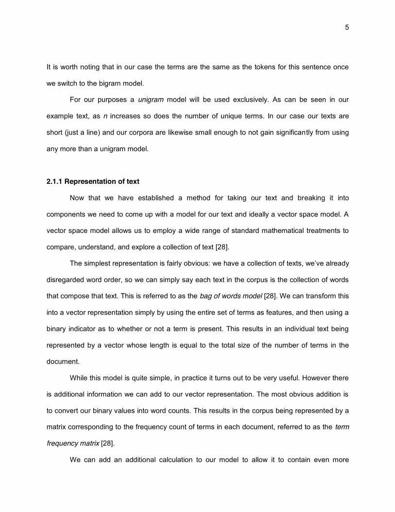
The simplest representation is fairly obvious: we have a collection of texts, we’ve already
disregarded word order, so we can simply say each text in the corpus is the collection of words
that compose that text. This is referred to as the bag of words model [28]. We can transform this
into a vector representation simply by using the entire set of terms as features, and then using a
binary indicator as to whether or not a term is present. This results in an individual text being
represented by a vector whose length is equal to the total size of the number of terms in the
document.
While this model is quite simple, in practice it turns out to be very useful. However there
is additional information we can add to our vector representation. The most obvious addition is
to convert our binary values into word counts. This results in the corpus being represented by a
matrix corresponding to the frequency count of terms in each document, referred to as the term
frequency matrix [28].
We can add an additional calculation to our model to allow it to contain even more

6
information. Rather than simply looking at how frequently a term appears in a specific document
we can also consider how frequently it appears in everything else. For example the word ‘the’
may appear 3 times in one text, but we know that this word will appear all over the corpus in
great frequency. However if we see the word ‘duplicitous’ appear 3 times, and we find that it
appears dramatically less frequently throughout the rest of the corpus then there might be
something interesting it tells us about this specific text. To factor this in we can use the inverse
document frequency (i.e. 1/total count of terms in the corpus). This allows us to quantify how
special a term is. Finally we can factor this into our frequency count which allows us to arrive at
our final vector space model, the term frequency - inverse document frequency matrix (tf-idf)
[17, 27, 28].
Our final vector space model, the tf-idf matrix, has some interesting properties. First it is
a high dimensional matrix, with the number of features equaling the number of unigrams (unique
words) in our text. The size of the feature space can easily be tens or even hundreds of
thousands of features. Additionally most of the values in our tf-idf matrix are going to be 0, since
most text only contain a small fraction of the total vocabulary. This is referred to as a sparse
matrix [28].
2.1.2 Determining Similarity Between Texts
The core of our project is comparing how similar texts are. Since we now have a vector
representation of our text we have available to us all of the distance metrics we have for
measuring any two vectors. An initial assumption would be to compare the distance in
Euclidean space. That is, we can treat each vector as a point in n-dimensional space (where n
is the size of the vocabulary) and simply calculate similarity as the distance between these two
points, p and q as represented by the following equation [59]:

7
d(q, p) = (p − q ) + (p − q ) + . . . + (p − q )
Unfortunately, due both to the sparsity and high-dimensionality of our matrix, Euclidean distance
gives us less desirable results [28]. But we need not give up mathematical simplicity in order to
arrive at our similarity metric. If we think of our vectors not as points but as hyper-planes we can
then look at the angle between them. To make this even cleaner we can simply take the cosine
between the two vectors and get a nice value between 0 and 1 which will indicate how similar
the documents are [28].
sim (d , d ) =d ⋅ d|d ||d |
2.2 Fractals
In his famous paper How long is the coast of Britain? Benoit Mandelbrot observed an
interesting fact about the coast of Britain [26]. If one is trying to measure the coastline, and
starts with a stick that is 200km long (Figure 2.1), you will find a length which would seem to
approximate the actual length of the coast, of course missing all the features that cannot be
measured by a 200km stick.
Figure 2.1: Measuring coast of Britain with a 200km measuring stick [55]
8
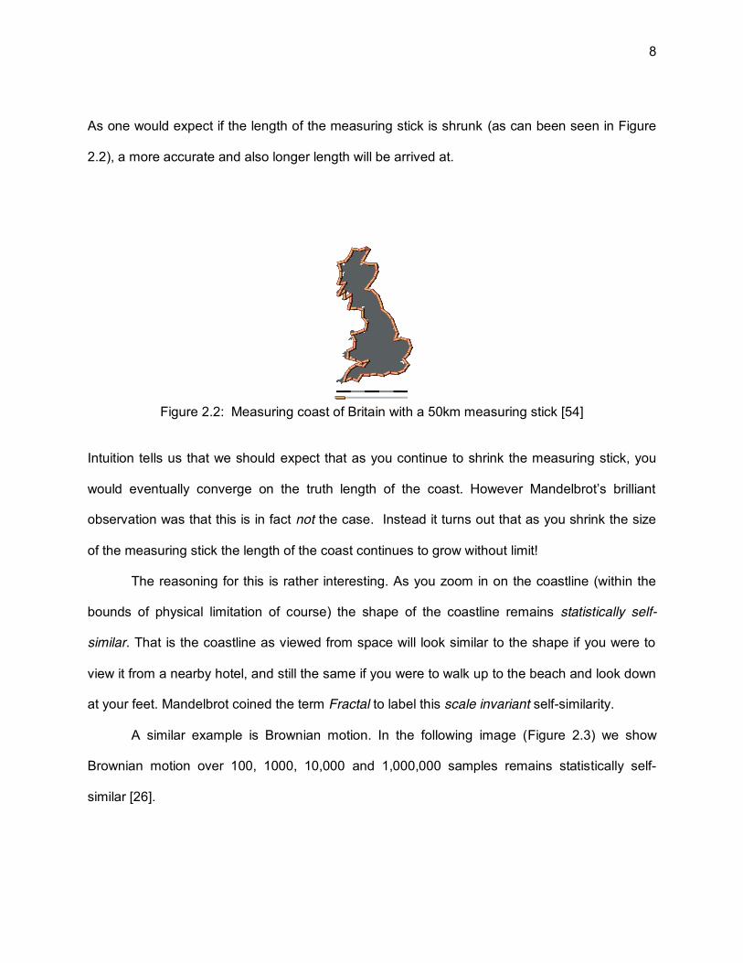
As one would expect if the length of the measuring stick is shrunk (as can been seen in Figure
2.2), a more accurate and also longer length will be arrived at.
Figure 2.2: Measuring coast of Britain with a 50km measuring stick [54]
Intuition tells us that we should expect that as you continue to shrink the measuring stick, you
would eventually converge on the truth length of the coast. However Mandelbrot’s brilliant
observation was that this is in fact not the case. Instead it turns out that as you shrink the size
of the measuring stick the length of the coast continues to grow without limit!
The reasoning for this is rather interesting. As you zoom in on the coastline (within the
bounds of physical limitation of course) the shape of the coastline remains statistically self-
similar. That is the coastline as viewed from space will look similar to the shape if you were to
view it from a nearby hotel, and still the same if you were to walk up to the beach and look down
at your feet. Mandelbrot coined the term Fractal to label this scale invariant self-similarity.
A similar example is Brownian motion. In the following image (Figure 2.3) we show
Brownian motion over 100, 1000, 10,000 and 1,000,000 samples remains statistically self-
similar [26].

9
Figure 2.3: Brownian motion at 100, 1,000, 10,000 and 1,000,000 samples
We can view the 100 samples as 1,000,000 samples zoomed in 10,000 times, and from these
images it is quite clear that there is no obvious difference, other than scale, in the shape of the
line. Just as the coast of Britain has the interesting property of being effectively of infinite length,
Brownian motion has the property of being everywhere continuous and nowhere differentiable
[26].
There are many patterns in mathematics that exhibit more obvious self-similarity, and
likewise strange properties [14, 40]. Take for example the Cantor set (Figure 2.4), which is
created by removing the middle third of a line, and then repeating this process with the two lines
created by removing this segment. Seven iterations of this process are visualized below [40,
56].

10
Figure 2.4: Cantor set [57]
This fractal behavior of the Cantor set leaves it with the interesting property of having a measure
of 0 while also being uncountably infinite [40, 56].
Another interesting geometric fractal is the Sierpinski gasket (Figure 2.5), which is
created by continually removing the middle triangle from a large triangle as seen below [14, 40,
68].
Figure 2.5: Sierpinski gasket [69]
The Sierpinski gasket is a great example of a fractal that can be embedded in a 2 dimensional
space.
2.2.1 Fractals in Nature
As the coastline of Britain suggests, fractals are abundant in nature. They appear
everywhere from vegetables (Figure 2.6), to music, to the structure of toddler scribbles (Figure
2.7) and the distribution of galaxies in the universe [14, 24, 26, 40, 62].

11
Figure 2.6: Romanesco cauliflower [58]
Figure 2.7: Doodles by Archer Kurt (age 3) compared to Levy flight
An obvious question that may arise when viewing fractals in nature is, “how exactly do we
define a fractal?” While there is no absolute definition of a fractal, the key features we look for
are self-similarity and scale invariance [14]. Other features that can be useful are: that it is too
irregular to be described in traditional geometric language, it has a fine structure, and it has a
fractal dimension greater than its topological dimension [14].
Since our work is dealing with visualizing song lyrics, the fractal properties are heavily

12
constrained by the very discrete and finite nature of our similarity matrices. Nonetheless we will
still be able to identify a variety of the features that strongly suggest a fractal nature in the
structure of certain songs and poems.
2.2.2 Measuring Fractals
Given that fractals have such curious properties as 0 measure yet uncountably infinite,
or a coastline that has unbounded growth as the instrument measuring it shrinks, an important
question to answer is how are they measured? If we go back to thinking about a measuring stick
we can start to approach an answer. Suppose we have N measuring sticks of the length r and
we’re trying to measure the circumference of a circle. We will have the following formula for the
approximate length (circumference) L of the circle.
L = N ⋅ r
And for a normal geometric shape like a circle, as r approaches 0 we arrive at a finite limit which
is the circumference of our circle.
lim →
N ⋅ r = L
The initial steps of this process are illustrated in Figure 2.8.

13
Figure 2.8: Approximating circumference of circle
But as discussed previously, the fact that for fractals N ⋅ r never converges is precisely what
makes them interesting. However it turns out that the growth of fractals can be described as a
power law of the form N ⋅ r where the rate at which the length grows is constant with respect
to D [14,24,26,40]. This exponent is referred to as the Hausdorff dimension and is the typical
way to measure a fractal. We can alternatively view the previous formula as [40]:
D := lim→
log Nlog(1/r)
Beyond simply being a way to measure fractal, the Hausdorff dimension tends to intuitively
correspond to the weird dimensionality of fractals [40]. For example the Sierpinski gasket
mentioned previously, which is a 2 dimensional set that has 0 measure and is uncountable has
a Hausdorff dimension of 1.58. This seems to make intuitive sense as the Sierpinski gasket is
not quite a 2 dimensional object, owing to its strange ‘emptiness’ and at the same time is
certainly not simply a 1 dimensional line. Similarly the Cantor set has a Hausdorff dimension of
only 0.6309, once again nicely representing its nature of being less than a standard 1
dimensional line.
14
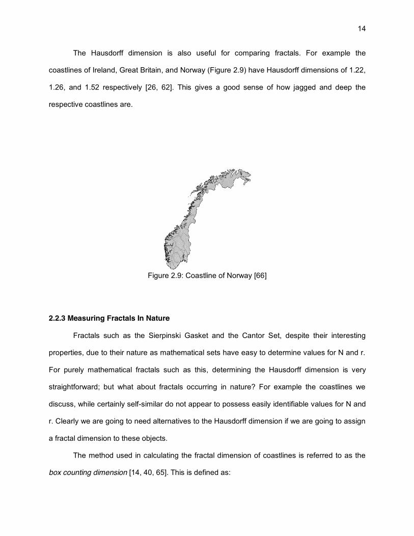
The Hausdorff dimension is also useful for comparing fractals. For example the
coastlines of Ireland, Great Britain, and Norway (Figure 2.9) have Hausdorff dimensions of 1.22,
1.26, and 1.52 respectively [26, 62]. This gives a good sense of how jagged and deep the
respective coastlines are.
Figure 2.9: Coastline of Norway [66]
2.2.3 Measuring Fractals In Nature
Fractals such as the Sierpinski Gasket and the Cantor Set, despite their interesting
properties, due to their nature as mathematical sets have easy to determine values for N and r.
For purely mathematical fractals such as this, determining the Hausdorff dimension is very
straightforward; but what about fractals occurring in nature? For example the coastlines we
discuss, while certainly self-similar do not appear to possess easily identifiable values for N and
r. Clearly we are going to need alternatives to the Hausdorff dimension if we are going to assign
a fractal dimension to these objects.
The method used in calculating the fractal dimension of coastlines is referred to as the
box counting dimension [14, 40, 65]. This is defined as:

15
D := lim→
log N(ε)log(1/ε)
This is nearly identical to the Hausdorff dimension, except this time we have replaced r with ε
where ε is the length of the side of a box. The method involves placing boxes with progressively
smaller sides (defined by ε) around the coast. As ε shrinks we continue to count the number of
boxes required to cover the coastline, which is N(ε). Eventually the ratio of the two logs will
converge to the box counting dimension D . A visualization of this can be seen in Figure 2.10.
Figure 2.10: Estimating the box counting dimension of the coast of Britain [60]
The box counting dimension works great for fractals that are similar to coastlines, which can be
represented as essentially a line; but what about fractals that are not easily represented by a
similar model? For example both goose down (Figure 2.11) and the Lichtenberg Figure (Figure
2.12) are fractal in nature [29], however cannot be easily measured by either the Hausdorff
dimension or the box counting dimension [40].

16
Figure 2.11: Goose down [44]
Figure 2.12: 3-D Lichtenberg figure in acrylic [67]
For these types of naturally occurring fractals we use the mass dimension [40]. This method
works by expanding a circle of a continually growing radius R and observing a number of
particles that are contained in the radius, which describes the mass M. Thus mass can be
described by the following formula:
M ∼ R
This translates into a very simple calculation for the mass dimension:
D ∼ log(M)log(R)

17
This then allows us to empirically calculate the fractal dimension of naturally occurring fractals
that are not easily measure by either the Hausdorff dimension or the box counting dimension.
The mass dimension will be an essential tool in exploring the dimension of the fractals that
emerge in lyrical verse.
When looking at the various methods of calculating the dimension of a fractal, the key
observation is that we’re always trying to understand the power law that governs the self-similar
growth of the fractal structure.
2.3 Visualizing Text
The most prominent work in text visualization in general comes out of the work of
Fernanda Viégas and Martin Wattenberg. Well known for their general work in the field of
information visualization with their Many Eyes [47] project as well as more recent work in
visualizing wind patterns [49], the team has also done popular work within the general domain of
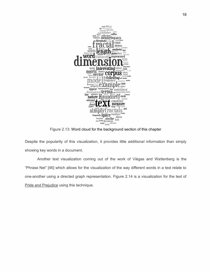
text visualization. Wordle, a tool for generating “tag clouds” [5, 48] has become a popular
method of visualizing text. Figure 2.13 is the Wordle tag cloud for the background section of this
chapter. As can plainly be seen the visualization works by highlighting key words in the text
document and arranging all of the generally important words into a ‘cloud’ shape.
18
Figure 2.13: Word cloud for the background section of this chapter
Despite the popularity of this visualization, it provides little additional information than simply
showing key words in a document.
Another text visualization coming out of the work of Viégas and Wattenberg is the
“Phrase Net” [46] which allows for the visualization of the way different words in a text relate to
one-another using a directed graph representation. Figure 2.14 is a visualization for the text of
Pride and Prejudice using this technique.

19
Figure 2.14: Phrase net for “Pride and Prejudice” [36]
Viégas and Wattenberg also produced a similar graph representation in their ‘Word Tree’ [50].
Rather than showing relationships between words the Word Tree acts as a visual concordance,
allowing those interacting with the visualization to observe all possible next words in a sentence
from a given word. An example taken from Martin Luther King’s “I have a dream speech” is seen
in Figure 2.15.

20
Figure 2.15: Word tree for “I Have a Dream” [70]
2.3.1 Other Examples of Text Visualization
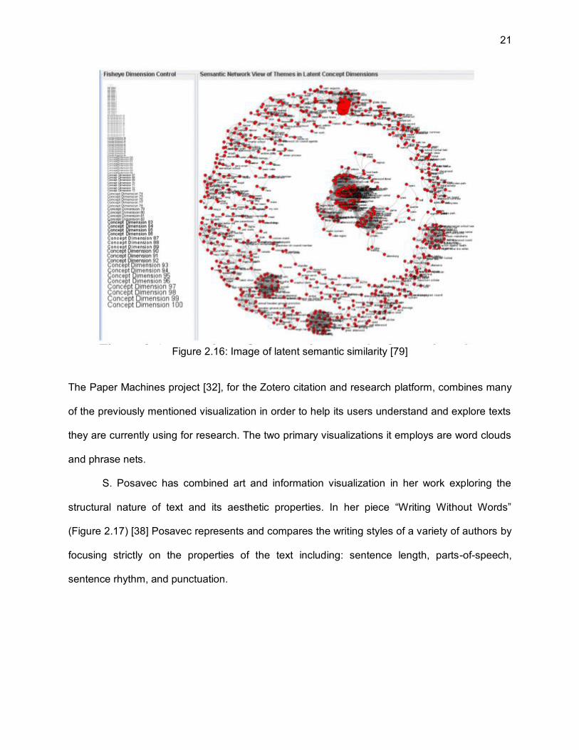
The Storylines project [79] attempts to use latent semantic analysis (LSA) to allow users
of the visualization to explore themes in unstructured text (Figure 2.16). LSA works by using the
Singular Value Decomposition (SVD) to project the very high dimensions tf-idf matrix onto a
lower dimensional subspace. One of the byproducts of this process is that features with similar
meaning will be projected near each other, and as a result a certain degree of semantics can be
inferred [28]. Once SVD is performed on the tf-idf matrix then terms are plotted in clusters to
create a semantic network. The aim of this visualization is that clusters of meanings will be
visible in the semantic network providing insight into themes present in the document.
21
Figure 2.16: Image of latent semantic similarity [79]
The Paper Machines project [32], for the Zotero citation and research platform, combines many
of the previously mentioned visualization in order to help its users understand and explore texts
they are currently using for research. The two primary visualizations it employs are word clouds
and phrase nets.
S. Posavec has combined art and information visualization in her work exploring the
structural nature of text and its aesthetic properties. In her piece “Writing Without Words”
(Figure 2.17) [38] Posavec represents and compares the writing styles of a variety of authors by
focusing strictly on the properties of the text including: sentence length, parts-of-speech,
sentence rhythm, and punctuation.

22
Figure 2.17: “Writing Without Words” [76]
Her work contains many other examples of similar explorations of the aesthetic nature of the
structure of text itself [37].
2.3.2 Visualizing Poetry and Song Lyrics
The work our project focuses on is strictly concerned with visualizing repetition in lyrical
verse. There are a variety of text visualization projects that concern themselves specifically with
poetry and song lyrics. Abdul-Rahman et al. examined a rules based system for visualizing
poetry [1]. Their project worked by visually representing a variety of features of the poem:
phonetic relations, phonetic features, words, and semantic relations. The result of their
technique on a sonnet can be seen in Figure 2.18

23
Figure 2.18: Visualizing a sonnet [1]
This work was then built into the Poem Viewer at the University of Oxfords e-Research Centre
(http://ovii.oerc.ox.ac.uk/PoemVis/index.html). The Poem Viewer allows users to upload poetry
and then interactively visualize the various components of the poem. Figure 2.19 gives a
screenshot of this interface.
Figure 2.19: Screenshot from POEM Viewer
Another researcher, Rhody, used the MALLET tool [25] in order to aid in the
understanding of specific collection of poems [39]. The project consists of using the MALLET
tools to perform topic modeling in order to identify potential topics in the corpus of 276 poems.
Rhody then utilized a series of standard charts and graphs to better understand the topic

24
modeling, and gain insight into themes present across poems in the corpus.
In 2005 the Group Lab at the University of Calgary did work in visualizing song lyrics as
they occur in a song in real-time [10]. The visualization works by highlighting each word as it is
sung, and then visually representing how long the word is vocalized by the singer with a growing
radius representing the duration that the word has been sung. Figure 2.20 shows this in action.
Figure 2.20: Screenshot of Group Lab’s lyric visualization
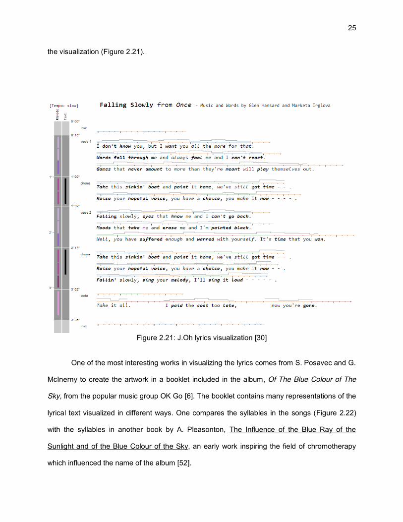
Another song lyric visualization project by J. Oh [30] seeks to improve the way that
musicians and performers can understand how song lyrics are incorporated into the larger work
of the song. Oh’s project tracks linguistic features, musical features, and the overall song
structure in order to aid the reader in understanding where and how specific sections of the
lyrics fit in with the rest of the song. Accented syllables are italicized, key words are bolded, the
pitch is represented as a step chart, and various other musical components are encoded into
25
the visualization (Figure 2.21).
Figure 2.21: J.Oh lyrics visualization [30]
One of the most interesting works in visualizing the lyrics comes from S. Posavec and G.
McInerny to create the artwork in a booklet included in the album, Of The Blue Colour of The
Sky, from the popular music group OK Go [6]. The booklet contains many representations of the
lyrical text visualized in different ways. One compares the syllables in the songs (Figure 2.22)
with the syllables in another book by A. Pleasonton, The Influence of the Blue Ray of the
Sunlight and of the Blue Colour of the Sky, an early work inspiring the field of chromotherapy
which influenced the name of the album [52].

26
Figure 2.22: OK Go booklet – syllable visualization [31]
Another visualization represents the various words in the lyrics and their parts of speech which
are represented by color (Figure 2.23).
Figure 2.23: OK Go booklet – parts of speech visualization [31]

27
While the aim of these visualizations is to create an aesthetic experience rather than to
necessarily provide information about the lyrics, this work demonstrates quite well that the
patterns of data in lyrical verse contain within themselves aesthetics properties.

28
Chapter 3
Visualizing the Structure of Repetition in Lyrical Verse
“You say I am repeating something I have said before, shall I say it again?”
-- T.S. Eliot, The Four Quartets
3.1 Overview
When analyzing lyrical works, whether poetry or songs, repetition plays a major part in
understanding the work. Repetition can manifest itself in many ways: rhyming verses, recurrent
themes, structured choruses, allusions to earlier works, attention to select words, and meter to
name a few. Typically, in the close reading of lyrical works there is no systematic way to
observe patterns of repetition and the reader is left to discover them only through the process of
careful note taking and continual rereading of works.
After many years of rereading T.S. Eliot’s “The Four Quartets”, and copious notes in the
margins pointing to other parts in the stanza or even the large poem, it became clear that there
must be a faster, more holistic way to view repetition in the work as an entirety. Perhaps even to
form a framework for tracking similarities in the structure of repetition across multiple works and
authors.
3.2 Visualizing Repetition
For the most part, the intersections between those who study the content of lyrical verse
and those who study computational models of text are small. As such there is a lack of attempts
to visualize this important feature of text. By far the most dominant methods of visualizing text
are to either represent it in a graph structure [1, 32, 38, 46, 50, 79] or to provide line level
annotations [1, 10, 30]. While the graph-based visualization allows for the visualization of much

29
of the connecting structure of text it is usually at the cost of losing sequential information about
this structure. Themes and some forms of repetition can be observed, but the actual structure of
repetition is lost. With the annotated line approach sequential information is preserved but at the
cost of losing a “big picture” view of the larger structure of the work. Attempts to blend these two
[1] end up with extremely dense representations that can be difficult to parse and understand
when trying to view repetition as a whole. The challenge our visualization tackles is concisely
capturing the structure of repetition within an individual work, so that this structure itself can be
easily studied. The primary aim of our visualization is to gain insight into how repetition is
constructed in lyrical verse.
While there are many forms of repetition in lyrical verse, a good place to start is focusing
on repetition that is already easy to deal with given the existing tools of Natural Language
Processing. For our present work our focus is the exploration of repetition that can be
expressed by determining the similarity in content using the cosine between vectorized
representations of text. By simply visualizing a matrix of cosine similarity using a color gradient
for values from 0 to 1, we are able to observe a surprising number of previously difficult to
observe patterns of repetition in lyrical works.
3.3 Why Visualize?
While we have hinted at some of the potential benefits of visualizing lyrical work, our
visualization technique elucidates two major areas of understanding the individual works:
qualitatively by adding an extra layer of insight into the work which can aid in the process of
close reading, and quantitatively by providing tools by which the lyrical work can be understood
through mathematical modeling.
3.4 Close Reading
Close reading [3] is essentially the approach to understanding literature which involves

30
focused study of the specific portions of the work, the language it uses, and its relation to the
overall structure of the work as a whole. Due to the focused nature of close reading it can be
particularly hard to observe the work as a whole. However this, somewhat paradoxically, leads
to the problem that the way each component relates to the whole can be difficult to see despite
being potentially very insightful. By visualizing the entire work in a relatively compact space our
visualization allows for the structure of the poem itself to be subject to close reading, something
that is otherwise difficult if not impossible to achieve. In Figure 3.1 and Figure 3.2 we see our
visualization for William Blake’s “Divine Image” [2] alongside the original text. Despite being a
short poem it can be easily seen that the structure of repetition in the poem is not inherently
obvious until it is visualized. As an example it is clearly seen from our visualization that the first
line is echoed throughout the poem, though rarely is it exactly reproduced.
Figure 3.1: Line similarity for William Blake’s “Divine Image”

31
Figure 3.2: Songs of Innocence - Divine Image [61]
In this way our visualization can serve as a valuable aid to understanding the stylistic use of
repetition as well as finding themes that may emerge in the work based around the use of
similar language.
3.5 Mathematics of Aesthetics
From a quantitative perspective this visualization allows viewers insight into something
novel, rather than merely aiding in existing analysis. By not simply observing the pattern of
repetition in an individual poem or song we can begin to, at a glance, observe patterns that
appear across multiple poems or songs. Since we are essentially visualizing a matrix of
numerically represented similarity, this then opens up lyrical verse to a wide range of
mathematical analysis.
While repetition in lyrical verse is often an essential component (especially in forms such
as popular music) an interesting paradox emerges when we start to think on the meta-level
about how the structure of repetition itself works. Patterns are by their nature predictable, but
repetition that is too predictable is boring. At the other extreme, repetition that is completely

32
unpredictable, i.e. without pattern, is immediately shut out by the listener. On the one end of
this spectrum we have a record perpetually skipping and the other we have pink noise. How can
we create a tradeoff between these two extremes? Certainly a simple compromise between the
two seems deeply flawed. As a mental exercise imagine a record of pink noise continuously
skipping. Such an experience would certainly be even less appealing aesthetically than either of
its components!
If we wish to model aesthetics we need to find a model of the world that simultaneously
allows for the emersion of complex patterns while remaining, ultimately, unpredictable.
Fortunately there is already a field of study which focuses explicitly on this phenomenon. In the
study of dynamical systems, i.e. Chaos Theory, we come across systems that while entirely
deterministic, vary extremely from initial conditions and whose development cannot be predicted
[40]. And of course the most familiar manifestation of this is the fractal.
Perhaps the greatest insight gained by visualizing repetition in lyrics is the clear
emergence of self-similarity in the structure of repetition within works containing very dense
structures of repetition. Looking at classic Dr. Seuss poems as well as a variety of popular
music we can not only begin to observe this fractal nature in lyrical verse but actually measure
it.

33
Chapter 4
Implementation
“It’s you, it’s you, it’s all for you Everything I do I tell you all the time” -- Lana Del Rey, Videogames
4.1 Preprocessing
Before any work can be done, first it is necessary to get the raw text data in a form that
can be used by a program. This process begins with manual annotation of the text. The most
fundamental preprocessing step is to manually remove all content from a text document which
is not directly related to a poem or song. For example: many collections of poetry in Project
Gutenberg contain introductions to poems or sections; all of these need to be removed before
the text can be processed.
Since we wish to be able to work with any sort of lyrical verse we need a methodology
that would generally be able to separate a body of work (e.g. in the case of music and album, or
in the case of poetry the larger poem itself or book containing smaller poems) from its
subdivisions (e.g. an individual song or a stanza). We want to extract each individual line from a
source of lyrical verse and annotate it with the work, and subdivision name (e.g. album-song-
verse, poem-stanza-line)
Another constraint is that potentially large amounts of plain text documents would need
to be hand annotated, this makes conventional markup choices, such as xml, suboptimal due to
the amount of time required to hand format the entire document. Since most text is coming from

34
sources like Project Gutenberg, in which titles and appropriate line breaks could be assumed a
simple way of marking up text was devised. Text surrounded by ‘==’ would set the work title,
and text surrounded by ‘__’ would set the subdivision title. Pseudo code for the algorithm for
consuming text is as follows:
while readline(): if line matches “==(.+)==”: set work_title to the value in between the ‘==’
else if line matches “__(.+)__”: set subdiv_title to the valu between “__” else if line is a character string: write work_title, subdiv_title, line to file else line contains nothing, ignore.
The text parsed in this manner is then outputted to a .csv file. A simple csv file is chosen
because many tools easily support this file type.
4.2 NLP
4.2.1 NLP Preprocessing
Once we have the data in a machine readable csv file we can now begin the process of
NLP work. We have done this in R using the packages ‘tm’ and ’lsa’ [15,16,71]. When we read
in the csv file output by our preprocessing steps the result is 3 columns of data: work name,
subdivision name, and the text for the line itself. Before we can do any work we need to perform
some basic clean up. All excess white space and all punctuation is removed and all strings are
transformed to lower case.
4.2.2 Common NLP Preprocessing Avoided
It is fairly common in Natural Language Processing to remove what are referred to as

35
stopwords from a text. Stopwords are common works such as ‘as’, ‘the’, and ‘and’. Typically
these words act simply as noise, detracting from words which give more information about the
text. Another common NLP preprocessing technique is stemming which attempts to
automatically truncate words. This would cause words such as ‘walked’ and ‘walking’ to be
reduced to the same root ‘walk’. While both of these steps are fairly common in any nlp pipeline
they are deliberately avoided in this case due to the density and deliberate nature by which
lyrical verse is constructed.
4.2.3 Vectorization
The key step is to create a vectorized representation of the text. To do this we need to
create a term-frequency inverse-document frequency (tf-idf) matrix. This representation allows
us to capture a great deal of information about our text data. Rather than simply calculating
either the Boolean presence of a word in a vector, or its raw frequency count, we can gather
more information into our vector by also taking into account the terms frequency times the
inverse of the number of times that term appears in other documents. This way the uniqueness
of a term in the corpus can also be represented. To automate this process we used the ‘tm’
package in R.
poem.dtm <- DocumentTermMatrix(poem.corpus,control = list(weighting =
function(x) weightTfIdf(x, normalize = FALSE), wordLengths=c(1,Inf)))
One important note on the code here is that the default behavior of the ‘tm’ package is to
remove words that are less than 2 characters. In the majority of NLP tasks this would be a
perfectly sensible decision. However, as we will see in the results sections, it is not uncommon
for a two character, or even a single character, word to have a large impact on the language of
the lyrical work. This is a recurring issue with NLP involving poetry, minutiae which is often
36
noise in large text documents is actually very useful information in poetry. The majority of text
preprocessing that is standard in most text vectorization processes is in fact detrimental when
working with a corpus in which each word, no matter how small, was likely chosen with
intention.
4.2.4 Sparse Representation
One of the challenges in working with text is the high dimensionality of the feature space
(which is the complete vocabulary of the corpus) of the vectorized representation. Because the
vast majority of words in the total feature space are not present in an individual line (which
frequently is only 5-6 words) we are left with an incredibly sparse matrix. To more efficiently
work with text data we keep our matrix represented in a sparse form, where each value is stored
at an index and all others are assumed to be 0. While this leads to a dramatically more efficient
representation there are often functions which require us to transform our data not only from
sparse matrix to full matrix, but also between different sparse representations based on what
different R packages expect data to look like.
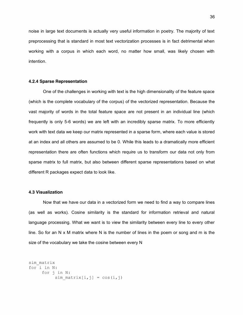
4.3 Visualization
Now that we have our data in a vectorized form we need to find a way to compare lines
(as well as works). Cosine similarity is the standard for information retrieval and natural
language processing. What we want is to view the similarity between every line to every other
line. So for an N x M matrix where N is the number of lines in the poem or song and m is the
size of the vocabulary we take the cosine between every N
sim_matrix for i in N: for j in N: sim_matrix[i,j] = cos(i,j)

37
Conveniently the R package ‘lsa’ [71] contains a function ‘cosine’ which will compute the cosine
between all column vectors. Because we want to compute the cosine between rows we simply
need to transpose the matrix and then transpose it back again:
sim.m <- t(cosine(t(as.matrix(poem.sm))))
Now we have an NxN matrix representing the similarity between every line with every other line.
This of course means that all items along the diagonal of this matrix will be perfectly similar
since this represents each line’s similarly with itself. There is also a mirroring effect in the
visualization since cosine(x,y) = cosine(y,x). While this does create redundant data in the
visualization, this redundancy does not necessarily detract from the ability to interpret the data
and, by providing an alternate perspective, may in fact enhance it.
One of the more interesting challenges was with orientation. In the first draft the lower
left corner was 0,0 as is typical for a Cartesian graph. However in showing this information to
public audiences one of the most common critiques was “Why are they backwards”? Although
using a standard Cartesian plane obviously made sense, we decided in the end to have the 0,0
coordinate located in the upper left corner. There are 2 major reasons for making this decision.
First, this is somewhat standard for the already popular correlation matrix, and most importantly
English speakers read from left to right, and top to bottom. Especially when juxtaposed with the
original poem this second method of visualizing the work seems radically superior.
Finally we need to actually create our visualization. Thanks to the powerful R
visualization library ‘ggplot2’ [51], this was relatively simple given that we had already created
our similarity matrix. Using the package’s qplot function and simply specifying the geometry to
be ‘tile’ our similarity matrix is automatically converted into an image such as Figure 4.1. Only a
few minor tweaks of graphical parameters were required to clean up the overall display.

38
Figure 4.1: Line similarity for Vampire Weekend’s “Ya Hey” [23]
4.4 Computing Fractal Dimension
Since our representation of text is necessarily discrete and only encompasses a rather
small scale it was essential to find a method of calculating the fractal dimension that would still
perform well given these constraints. For this we chose to use the mass dimension (details in
Chapters 2 & 5) which attempts to infer fractal dimension by estimating the power relationship
between a radius r and the mass M representing the mass of points contained within an
increasing radius.
One of the key implementation differences between representing similarity in this
calculation was the necessity of choosing a threshold for ‘similarity’ which would decide which
points were included in the mass calculation. In our visualization the entire spectrum from 0 to 1
could be represented, however for the sake of calculating mass we stuck with threshold of 0.5
based simply because it seemed to most honestly represent the similarity observed. Once a
threshold is set then the distance between each point is calculated from an origin (almost
always the last line in the song) which visually appeared to be the origin of the fractal.
distances.of.points <- sapply(1:length(points.x),function(i){ sqrt((points.x[i]-o.x)^2 + (points.y[i]-o.y)^2) })

39
Then for a discrete range of radii, the algorithm simply collects how many points are closer to
the center than r (i.e. which points are contained in the radius).
point.count <- sapply(radii,function(r){ sum(distances.of.points < r) })
Now we have a collection of points the sequence of radii as well as corresponding mass for
each. We then used linear regression to find the approximate slope of these lines. To do this we
used R’s glm function which creates a generalized linear model for the log of the masses and
radii. Taking the log of each is necessary since the exponential growth can then be represented
as linear growth.
Rather than using ordinary least squares (OLS), we used iteratively reweighted least
squares (IRWLS). IRWLS unlike OLS does not assume a consistent variance between the x
and y values. This ends up weighing the denser cluster of values more strongly than the initial
set. This is useful for two reasons. First, due to the discrete nature of the values it is visibly clear
that the initial points have much higher variance; second, due to the log transformation the
points at the end of the sequence are more densely clustered.
4.4.1 Visualizing Fractal Dimension
The visualization for the mass dimension calculation consists of two parts. The first,
show in Figure 4.2, visualizes the computation process showing how progressively large radii
enclose increasing more of the mass.

40
Figure 4.2: Calculating the mass dimension
The second visualization, shown in Figure 4.3, is simply the log-log plot of M to r with the linear
regression line showing the slope between the two points (which is the approximate fractal
dimension).
Figure 4.3: Log-log plot for approximating mass dimension
Both of these plots were created with R’s built-in plotting functionality.

41
Chapter 5 Results
“Karma police, arrest this man He talks in maths He buzzes like a fridge He's like a detuned radio” -- Radiohead, Karma Police
5.1 Visualization - Simple Applications
The original motivation for this visualization was the observation that when reading
larger poems it became exceedingly difficult to track themes and repeated lines throughout the
entire work. Close reading of a text is typically focused on only a small section of the work at a
time. Understanding the relationship a given section has to another can be tremendously
important to understanding the work as a whole and even special significance an individual
subsection may have because of the role it plays with other subsections. As more of these
visualizations were created it became apparent that this was also an issue even in smaller,
denser works. In the following sections, we explore how close reading can be aided by viewing
the structure of repetition. We also explore how one can focus strictly on the structure of lyrics in
a song, and essentially use the lyrics to understand the structure, inverting the process in the
first example.
5.1.1 Visualizing the Thunder - Visualization and Close reading
Without the aid of visualization it is very hard to arrive at a holistic view of meaningful
patterns of repetition in a work. One of the most valuable functions of these visualizations is
they allow expansion upon traditional close reading. For example, let us look at the final section

42
of T.S. Eliot’s The Wasteland [12]. The section is titled “What the Thunder Said”. Figure 5.1 is
the line similarity visualization for this section.
Figure 5.1: Line similarity for T.S Eliot’s “The Wasteland - what the thunder said”
Here we see the common pattern of a single primary cluster of repetition, in this case at the
beginning of the section. Taking a look at the early parts of the poem we can see where in the
text some of this repetition is occurring:
If there were water And no rock If there were rock And also water And water

43
A spring A pool among the rock If there were the sound of water only Not the cicada And dry grass singing But sound of water over a rock Where the hermit-thrush sings in the pine trees Drip drop drip drop drop drop drop But there is no water
The words which are causing most of the repetition are ‘water’ and ‘rock’. Particularly interesting
is that this passage, ending with the lament “But there is no water”, is also the end of repetition.
It is not much of a stretch to point out that the repetition of words replicates the “pitter patter” of
water on rocks, of rain drops. This can literally be seen in the text when visualized. Something
that is not obvious without the visualization.
When looking for further repetition something truly fascinating sticks out. Near the end of
the passage the repetition of language starts to return, most clearly evident in the 6 solid dots
appearing in the last section (Figure 5.2).
Figure 5.2: Close-up of “DA” section
These 3 lines (6 dots due to the mirroring effect) are actually one single word repeated: ‘DA’. To
truly see what is interesting it is important to understand their context:
Then spoke the thunder DA

44
The sound ‘DA’ which is the focus of the repetition in this section is the voice of the thunder, the
sound of a coming storm. Looking back at the overall picture we see the transition from imagery
of water, to its absence, to its eventual return. All of this is in fact visible simply from the pattern
of repeated words. We can observe the cloud dissipate and reemerge with the sound of
thunder.
5.1.2 Understanding the Structure of Popular Songs
While poetry has relied heavily on repetition and recurring themes, the tendency towards
repetition in song lyrics is even stronger. Not only do choruses and refrains create segments of
perfect repetition, it is not uncommon to find a series of phrases that continue being slightly
altered in progression. We can see this in the example of Vampire Weekend’s song ‘Walcott’,
illustrated in Figure 5.3 [22].
Figure 5.3: Line similarity for Vampire Weekend’s “Walcott”
45
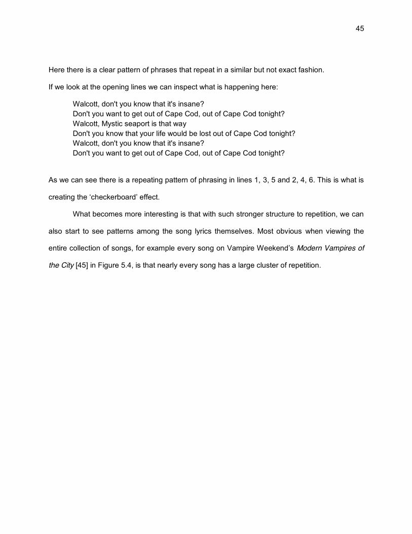
Here there is a clear pattern of phrases that repeat in a similar but not exact fashion.
If we look at the opening lines we can inspect what is happening here:
Walcott, don't you know that it's insane? Don't you want to get out of Cape Cod, out of Cape Cod tonight? Walcott, Mystic seaport is that way Don't you know that your life would be lost out of Cape Cod tonight? Walcott, don't you know that it's insane? Don't you want to get out of Cape Cod, out of Cape Cod tonight?
As we can see there is a repeating pattern of phrasing in lines 1, 3, 5 and 2, 4, 6. This is what is
creating the ‘checkerboard’ effect.
What becomes more interesting is that with such stronger structure to repetition, we can
also start to see patterns among the song lyrics themselves. Most obvious when viewing the
entire collection of songs, for example every song on Vampire Weekend’s Modern Vampires of
the City [45] in Figure 5.4, is that nearly every song has a large cluster of repetition.
46
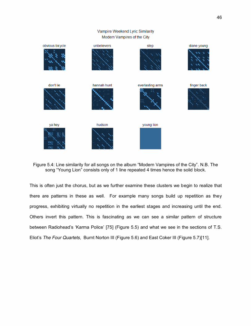
Figure 5.4: Line similarity for all songs on the album “Modern Vampires of the City”. N.B. The song “Young Lion” consists only of 1 line repeated 4 times hence the solid block.
This is often just the chorus, but as we further examine these clusters we begin to realize that
there are patterns in these as well. For example many songs build up repetition as they
progress, exhibiting virtually no repetition in the earliest stages and increasing until the end.
Others invert this pattern. This is fascinating as we can see a similar pattern of structure
between Radiohead’s ‘Karma Police’ [75] (Figure 5.5) and what we see in the sections of T.S.
Eliot’s The Four Quartets, Burnt Norton III (Figure 5.6) and East Coker III (Figure 5.7)[11].

47
Figure 5.5: Line similarity for Radiohead’s “Karma Police”
Figure 5.6: Line similarity for “Burnt Norton III”

48
Figure 5.7: Line similarity for “East Coker III”
At this point it should be clear that there are many observations about the structure of lyrical
representation that benefit from visualizing the cosine similarity of the documents. Even more
striking is the ease with which repetition can be compared across genres and authors. Seeing
similar patterns in repetition between Eliot and Vampire Weekend is something that would be
very difficult to achieve analyzing only the text itself.
5.2 The Fractal Nature of Lyrical Verse
Starting from the simple observation that there are recurring patterns of similarity across
a wide range of lyrical verse, we stumble across an even more startling observation. Among
these families of patterns we actually come across many that are truly fractal in nature. This is a
significant insight in that it provides a much deeper understanding of why and how the
mechanics of repetition are able to create aspects of the aesthetic experience.
5.2.1 Green Eggs and Ham and Self-Similarity
One of the most fascinating insights provided by visualizing lyrical verse is what appears

49
when we start looking at either song lyrics with repeated chorus and verses or very repetitive
dense poetry such as is typically found in books of children's verse. The most striking of these is
Dr Seuss’s classic “Green Eggs and Ham” (Figure 5.8) [42]. For those unfamiliar with the work
one of the key structural components is the building up of an enumeration of conditions in which
the central character will not eat green eggs and ham:
I could not, would not, on a boat. I will not, will not, with a goat. I will not eat them in the rain. I will not eat them on a train. Not in the dark! Not in a tree! Not in a car! You let me be! I do not like them in a box. I do not like them with a fox. I will not eat them in a house. I do not like them with a mouse. I do not like them here or there. I do not like them ANYWHERE!
This list is creating a recurring pattern of repetition. Along with other mechanisms of repetition
within the larger poem this leads to a particularly striking visualization.

50
Figure 5.8: Line similarity for “Green Eggs and Ham”
Aside from the sheer complexity of the structure of repetition there is something else which is
very crucial to truly understanding the significance of this structure. The careful observer will
notice that the square pattern between lines 1 through approximately line 40 is self-similar to the
structure over the rest of the work (Figure 5.9).

51
Figure 5.9 Zoomed in segment of “Green Eggs and Ham” (compare with entire document in
Figure 5.8)
Not only is the self-similarity present between the beginning and the body of the work but
something we see all over at various scales (highlighted in Figure 5.10). This self-similarity
across scales implies that the structure of repetition in “Green Eggs and Ham” is in fact fractal in
nature.

52
Figure 5.10: Highlighted self-similarity in “Green Eggs and Ham”
This is quite an astounding discovery and has broad implications for how the aesthetics
of repetition actually work. We’re used to seeing fractals imagined in a variety of natural
phenomenon from finance to cauliflower but without visualization it certainly not clear that the
mechanics of children’s poetry may in fact be driven by a hidden fractal.
Taking other examples from Dr. Seuss’s body of work, with an eye open for self-
similarity, we come across more self-similarity, though not as obvious as in of “Green Eggs and
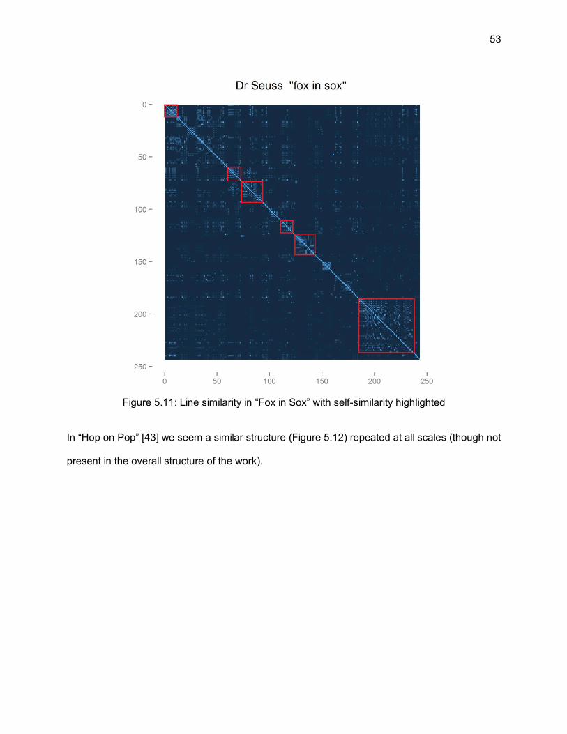
Ham”. In “Fox in Sox” [41] there is a common pattern of a dense cluster followed by sparser
areas of repetition (Figure 5.11). This pattern is somewhat apparent in work as a whole but also
appears, sometimes with reversed orientation throughout the poem.
53
Figure 5.11: Line similarity in “Fox in Sox” with self-similarity highlighted
In “Hop on Pop” [43] we seem a similar structure (Figure 5.12) repeated at all scales (though not
present in the overall structure of the work).

54
Figure 5.12: Line similarity in “Hop on Pop” with self-similarity highlighted
Not every Dr. Seuss poem presents itself as a fractal quite as clearly as “Green Eggs
and Ham”; however we consistently find the presence of some degree of scale invariant self-
similarity. More than mere curiosity, this provides insight into the way fractals might work to
structure repetition in order to create an overarching aesthetic.
5.2.2 Searching for Fractals in Song Lyrics
The reason that we are able to so easily identify fractals in works such as “Green Eggs
and Ham” is that the density of the repetition is more extreme than a work such as “Four
Quartets”. In order to continue our search for fractal patterns in lyrical verse, looking at lyrics in
popular music is likely to be another source rich in dense repetition.

55
Most popular music contains lyrics that work on a common theme and make heavy use
of repeated chorus and very similar verses which echo each other. One of many examples of
this echoing effect (with both exact and similar repetition) can be seen in Tame Impala’s “Why
Won’t They Talk to Me” [35]
Out of this Zone, trying to see, I’m so alone, nothing for me I guess I’ll go home, try to be sane, try to pretend, none of it happened … Out of this zone, Now that I see, I don’t need them and they don’t need me I guess I’ll go home, try to be sane, try to pretend, none of it happened
Given how common similar lyrical structure is to popular music we should expect to see much
stronger patterns in repetition (Figure 5.13).
Figure 5.13: Line similarity for Tame Impala’s “Why Won’t They Talk to Me”
And as expected line similarity in the visualization of “Why Won’t They Talk to Me” certainly has
a stronger visual repetition. However, it seems reasonably clear here, that what we are seeing
possesses no obvious self-similarity.

56
We don’t have to look too far, however to find songs that do exhibit more obvious self-
similarity. In “Feels Like We Only Go Backwards” [48] (Figure 5.14) what we see, noted by the
numerous bright spots, is that almost all of this self-similarity is created through the repetition of
the chorus which appears as follows:
chorus verse chorus verse chorus chorus chorus
When we look at the actual text of the chorus:
It feels like I only go backwards, lately Every part of me says go ahead I got my hopes up again, oh no, not again Feels like we only go backwards darling
We see that there is a sub-repetition in the chorus itself between the nearly identical (but not
perfectly identical) first and last lines.
Figure 5.14: Line similarity for Tame Impala’s “Feels Like We Only Go Backwards”

57
Not only does the repetition form an interesting pattern but we once again see scale invariant
self-similarity. To see this clearly, look at the box surrounded by a border formed in the lower
left, then notice that this box itself is followed by a similar border.
Perhaps more interesting are cases in which inner structure of a verse is used to create
self-similarity with the overall structure of the chorus. In “Feels Like We Only Go Backwards” the
primary function of the verses in the pattern is to create essentially white space so that the
larger pattern created by the chorus can emerge.
In Vampire Weekend’s “Obvious Bicycle” [20] we find a more sophisticated pattern of
repetition (Figure 5.15), in which the first 10 lines mirror the similarity structure of the chorus.
Figure 5.15: Line similarity for Vampire Weekend’s “Obvious Bicycle”
The self-similarity is highlighted in Figure 5.16 for clarification

58
Figure 5.16: Vampire Weekend’s “Obvious Bicycle” with self-similarity highlighted
It is worth noting that while “Obvious Bicycle” and “It Feels Like We Only Go Backwards” both
exhibit a clearly fractal structure with exemplified scale-invariance, the direction that invariance
progresses through the song is different. In “Obvious Bicycle” as the song progresses we
effectively magnify the first section, whereas in the “It Feels Like We Only Go Backwards” we
see the opposite scaling effect (that of “zooming out”). This further adds to an understanding of
ways in which fractal behavior can generate different aesthetic properties.
Looking through an increasingly large collection of songs we continue to come across
obvious fractals. What become particularly interesting are the fractal patterns that begin to
emerge across various songs. Take a look at Radiohead’s “Subterranean Homesick Alien” [77]
from the album OK Computer (Figure 5.17).

59
Figure 5.17: Line similarity for Radiohead’s “Subterranean Homesick Alien”
And then compare that with another song from the same album “The Tourist” [78] (Figure 5.18).
Figure 5.18: Line similarity for Radiohead’s “The Tourist”
Here we see an instance of self-similarity which occurs not within a single song but across many
others. Again we can see this same pattern emerge on Radiohead’s prior album The Bends in

60
“Bullet proof… I wish I was” (Figure 5.19) [73].
Figure 5.19: Line similarity for Radiohead’s “Bullet proof …. I wish I was”
And again we see a similar pattern on the album in the song “High and Dry” (Figure 5.20) [74].
Figure 5.20: Line similarity for Radiohead’s “High and Dry”
Even though the pattern in “High and Dry” is very similar to the other 3 examples from
Radiohead, we also get a glimpse of this same pattern starting to fall into a pattern of self-
similarity. The scale invariance is seen in the bordered rectangle in the right-left corner

61
expanding in a similar fashion as its own border becomes the end of the square in the next
series of repetition.
Not only do we see repetition in the very structure of repetition within one artist’s works,
but across multiple music groups. Here we can see a very similar pattern emerging between
Vampire Weekend’s “Hudson” (Figure 5.21) [19] and Lana Del Rey’s “Million Dollar Man”
(Figure 5.22) [8].
Figure 5.21: Line similarity for Vampire Weekend’s “Hudson”
Figure 5.22: Line similarity for Lana Del Rey’s “Million Dollar Man”

62
And again between “Feels Like We Only Go Backwards” (Figure 5.23) [33] and Lana Del Rey’s
“Radio” (Figure 5.24) [9]
Figure 5.23: Line similarity for Lana Del Rey’s “Radio”
Figure 5.24: Line similarity for Tame Impala’s “Feels Like We Only Go Backwards”
This repetition of fractals seems to imply that the repetition driving song lyrics follow a self-
similar pattern, but also across popular music in general we can expect to see a broader system
of self-similar representation. That is, a common set of fractals are able to create a broad range

63
of lyrical verse.
5.2.3 Song Lyrics and Cantor Dust
Perhaps the most dominating repeating pattern of repetition is a series of squares, which
without a larger context do not seem to obviously invoke a fractal. A wide range of songs from
an equally wide range of artists demonstrate this ‘boxy’ repetition. This pattern can be seen in
Lana Del Rey’s “Diet Mountain Dew” (Figure 5.25), Radiohead’s “Climb Up the Walls” (Figure
5.26), Vampire Weekend’s “one” (Figure 5.27), and Radiohead’s “Ripcord” (Figure 5.28) [7, 21
,72, 76].
Figure 5.25: Line similarity for Lana Del Rey’s “Diet Mountain Dew”

64
Figure 5.26: Line similarity for Radiohead’s “Climb Up the Walls”
Figure 5.27: Line similarity for Vampire Weekend’s “one”

65
Figure 5.28: Line similarity for Radiohead’s “Ripcord”
Not only do these images evoke similarity to each other but we also find them strikingly similar
to a well-studied fractal “Cantor Dust” (Figure 5.29) [40, 56]. Cantor Dust is created by taking
the cross product of cantor sets.
Figure 5.29: Cantor dust [55]

66
Given the image above it’s easy to retrospectively go back and find ways to match the lyrical
repetition to segments of the dust.
5.3 Measuring Fractals in Lyrical Verse
One of the most interesting and essential features of fractals is determining their
dimensionality. In the previous sections we have shown clear evidence that the structure of
repetition in dense lyrical verse frequently produces objects with fractal-like properties. In the
general case we can think of the fractal dimension as the way that m repetitions of a pattern
scale by a factor of r [14, 26, 40].
The standard way of measuring fractal is using the Hausdorff dimension described in the
following formula [6, 14, 24, 40]:
D := lim→
log Nlog(1/r)
Generally we can consider the Hausdorff dimensions as describing the rate that the length of
the fractal, N, scales exponentially with r. The Hausdorff dimension is particularly useful when
dealing with mathematically defined fractals (see chapter 2 for details).
Since we’re dealing with fractals observed in nature, which are discrete, and their scale
is bounded, we are going to have to rely on an empirical method of determining their fractal
dimension. For our purposes we are going to use the mass dimension [40] which asserts that
for mass M and radius R, with a dimension D:
M ≈ R
This in turn means that:

67
D ≈ log(M)log(R)
We can empirically calculate D by observing how M changes as R increases. We can see three
examples of calculating the mass dimension of the observed fractals in Figure 5.30.
Figure 5.30 Computing the mass dimension of (a) Tame Impala’s “It is not meant to be” (b) Vampire Weekend’s “Cousins” and (c) Lana Del Rey’s “Radio”. On top is the visualized
expanding value of R, and the bottom we see the log-log plot of M to R
In the Figures displayed [9, 18, 34] we see a visual representation of the radius R expanding
around the fractal component of the lyrics. Below this visualization is then the log-log plot of M
and R. By using linear regression we are able to estimate the power law that is driving the
fractal growth.

68
5.4 Interpreting the Fractal Dimension of Lyrics
At this point an obvious question to ask is, "What does it mean for lyrical repetition to
have 1.38 dimensions?" The answer to this question is actually at the heart of why these fractals
are interesting and useful in the first place. Non-integer dimensions typically embody the fact
that while a fractal may be embed in a specific dimension, or resemble one; it has properties
that seem counter intuitive. Take for example Mandelbrot's initial paper on measuring the coast
of Britain. The basic idea is that if we start with a measuring stick of say size 'n' (i.e. 1 meter) we
find one length for the coast, as n decreases we would expect the coastline measurement to
converge on a true length of the coast. But because the coastline's dimension is closer to 1.29
this is not actually what happens. Instead we find that the coast continues to expand in length!
To get a better sense of this, we will look at similar dimension calculations for prose. In
this case a segment taken from Jacques Ellul’s The Technological Society [13]. In Figure 5.31
we see this representation using the same threshold for similarity that we used for our song
lyrics. As can be seen this finds the passage to be completely without similarity. However this
representation is a bit unfair to the prose since there are plenty of recurring ideas and themes in
this passage, but the sentences are more complicated (and lengthier). To correct this, in Figure
5.32 we see the plot for the reduce threshold which lets us see some of the sentences which do
have repetition in content. In this latter representation we see that the text’s dimension is
approximately 1.

69
Figure 5.31 Calculating the mass dimension for a section from The Technological Society using the same threshold for similarity as all of the lyric calculations.
Figure 5.32 Calculating the mass dimension for a section from The Technological Society using a more relaxed threshold.
We can think of the default stream of speech, with no special repetition as a 1

70
dimensional line. But songs are special precisely because they are non-linear in the same way.
Exactly what makes lyrics, with repeated choruses and verses so appealing is this extra-
dimensionality. Poetry and especially song lyrics are different from prose in essentially the same
way that the coast of Britain is different from the Nevada/Utah border. In this way by
understanding the fractal nature of lyrical verse we begin to unravel the mathematics of
aesthetics.

71
Chapter 6 Conclusion
“In my end is my beginning.”
-- T.S. Eliot, The Four Quartets
6.1 Conclusion
In 1933 George Birkhoff, primarily known for his work on Ergodic theory, a field of
dynamical systems, wrote what has become a relatively obscure work titled Aesthetic Measure
[4]. In this work Birkhoff attempts to find a mathematical model of aesthetics. His initial model
determines that the aesthetic measure M is composed of two main components order O and
complexity 𝐶 and that aesthetic measure can be understood with this simple formula:
M = OC
To really understand what Birkhoff is getting at it is essential to expand on what is meant by
‘order’ and ‘complexity’. Complexity relates to the “feeling of effort” in perceiving the aesthetic
experience. For example a harmony with a very few distinct notes requires very little effort on
behalf of the listener, the more complex the music becomes the more tension is created for the
listener. For defining order Birkhoff lists a series of element which he considers to be ‘positive’:
repetition, similarity, contrast, equality, symmetry, balance, and sequence; and a series of
element he considers ‘negative’: ambiguity, undue repetition, and unnecessary imperfection. He
points out the jarring experience of a single wrong note appearing the middle of a performance

72
and an example of ‘unnecessary imperfection’, and an overall example of when order is lacking
in the aesthetic experience.
While there is little doubt that much nuance is missing from Birkhoff’s analysis, there is
an essential point which is useful in understanding the results from visualizing the structure of
lyrical verse. Aesthetics is a balancing act of trying to create order without overly taxing the
attention of the observer. This is precisely why our visualizations are essential to understanding
the true aesthetic nature of lyrical verse: the patterns that lead to the aesthetically pleasing
nature of verse must remain hidden from the audience to maximize the balance between order
and complexity.
Perhaps the most important insight gained in our work is not simply that there are fractal
patterns that drive the structure of lyrical verse, but specifically that there are hidden patterns
that need to be coaxed out of the work to be understood. As a counterpoint take the fairly
ubiquitous Mandelbrot set (Figure 6.1).
Figure 6.1: Mandelbrot set [63]
This image is, for many people, the definitive image of what a fractal is. It is certainly
aesthetically appealing, but we would argue not nearly as appealing as one’s favorite poem or

73
song. And yet we have found what are quite clearly fractal patterns in the lyrical structure of
popular verse, so what makes one fractal more appealing than another? To account for this we
only need to observe the visible complexity of the Mandelbrot set, which possesses a profound
order but at the cost of extreme complexity. The lyrical verses we have visualized only display
this complexity when we intentionally dig it out. The order created by these fractal patterns is
observed, while the aesthetic experience is heightened because the complexity driving this is
hidden from the observer.
The great value of visualizing similarity in lyrical verse is that it brings out the unseen but
essential structure of these works. The lesson for continued mathematical understanding of
aesthetics is to seek the very likely hidden processes that drive a beautifully simple order.
6.2 Future Work
6.2.1 Modeling Other Aspects of Repetition
The most obvious deficit in our current research is that we only focus on a very specific,
relatively small portion of the overall structure of repetition. Our work remains concerned with
only the reuse and repetition of exact words. Other forms of repetition certainly worth exploring
include: repetition of sounds, word meaning and themes, and meter. Approaches to each of
these would pose considerably more difficult challenges, especially ones pertaining to the
meaning of language.
6.2.2 Website for Aggregation
Perhaps the most useful future work would be to simply create a web presence where a
continually large sample of lyric visualization could be stored and explored. Certainly larger
structures of patterns would emerge as a larger and larger collection of visualization was stored.
74
Part of such a project could also include tools for the automatic processing and visualization of
user uploaded texts. Creating a community of users interested in lyrical patterns and continually
expanding knowledge in the area would be a tremendous benefit.
Another feature which would be great to add would be user interaction. Being able to
interactively highlight repetition and display which specific text corresponded to which moment
of repetition would likely provide even greater insights that we have explored here.
6.2.3 Generative Models
If the true aim is to gain a deeper understanding of aesthetics, there can be no truer text
that to eventually generate lyrics using models created from the patterns we have collected and
observed. More research would need to be done in the aforementioned forms of repetition not
covered to successfully generate complete texts. However even generating similar forms and
patterns that we have observed could be extremely useful and insightful.
6.2.4 Generalization
While the current work is focused specifically on text and text similarity the work in this
paper can be generalized to virtual any set of ordered data. The generalization works as follows:
Given an ordered set of data (in this case lines of text) which can be represented by a vector
(here rows in a tf-idf matrix) and a similarity function (e.g. cosine similarity) a similarity matrix
can then be trivially constructed and visualized using the exact technique used to visualize
similarity between lines in lyrical verse. This generalization opens the doors to performing
similar analysis on nearly any sequential data, from frames in a motion picture to moves in a
game of chess.
75
Bibliography [1] A. Abdul-Rahman, J. Lein, K. Coles, E. Maguire, M. Meyer, M. Wynne, C. R. Johnson, A.
Trefethen, and M. Chen. Rule-based Visual Mappings - with a Case Study on Poetry Visualization. Computer Graphics Forum, 32(3), 2013
[2] W. Blake. Divine Image, Poems of William Blake. Project Gutenberg, 1996 [3] G. Blank, M. Kay. The Close Reading of Poetry (Accessed April 6, 2014).
http://web.uvic.ca/~englblog/closereading/ [4] G. Birkhoff. Aesthetic Measure. Harvard University Press, 1933 [5] C. Collins., F. Viegas, M. Wattenberg. Parallel Tag Clouds to Explore and Analyze Faceted
Text Corpora. Proceedings of the IEEE Symposium on Visual Analytics Science and Technology (VAST 2009), IEEE, 2009
[6] Cover Art of the Week #9: Of the Blue Colour of the Sky, OK Go (Accessed April 5th 2014).
http://blog.aupeo.com/post/381650069/cover-art-of-the-week-9-of-the-blue-colour-of-the [7] L. Del Rey, J. Parker. Diet Mountain Dew, Born To Die. Polydor, 2012 [8] L. Del Rey, C. Braide. Million Dollar Man, Born To Die. Polydor, 2012 [9] L. Del Rey, J. Parker. Radio, Born To Die. Polydor, 2012 [10] R. Diaz-Marino, S. Carpendale, S. Greenberg. Lyric Text. Report iLab-2005-1, Dept.
Computer Science, University of Calgary, 2005 [11] T. Eliot. T.S. Eliot: Collected Poems, 1909-1962. Harcourt Brace Jovanovich, 1991 [12] T. Eliot. The Wasteland. Project Gutenberg, 1998 [13] J. Ellul. The Technological Society. Alfred A. Knopf, Inc., 1964 [14] W. Falconer. Fractal Geometry. Wiley, 2nd Edition, 2003 [15] I. Feinerer, K. Hornik, D. Meyer. Text Mining Infrastructure in R. Journal of Statistical
Software 25(5), 2008 [16] I. Feinerer, K. Hornik. tm: Text Mining Package. R package version 0.5-10. 2014
76
[17] K. Jones. A statistical interpretation of term specificity and its application in retrieval, Journal of Documentation. Vol 60. No. 50 2004 (reprint of Vol 28, no.1 1972)
[18] E. Koening. Cousins. Contra, XL Recordings, 2009 [19] E. Koening. Hudson. Modern Vampires of the City. XL Recordings, 2013 [20] E. Koening. Obvious Bicycle. Modern Vampires of the City. XL Recordings, 2013 [21] E. Koening. One. Vampire Weekend, XL Recordings, 2008 [22] E. Koening. Walcott. Vampire Weekend, XL Recordings, 2008 [23] E. Koening, R. Batmanglij. Ya Hey. Modern Vampires of the City. XL Recordings, 2013 [24] C. Madden. Fractals in Music. High Art Press, 2nd Edition, 2007 [25] MALLET (Accessed April 5, 2014). http://mallet.cs.umass.edu/ [26] B. Mandelbrot. How long is the coast of Britain? Statistical self-similarity and fractional
dimension. Science, 156, 1967 [27] C. Manning, H. Schütze. Foundations of Statistical Natural Language Processing. MIT
Press, 1999 [28] C. Manning, P. Raghavan, H. Schütze. Introduction to Information Retrieval. Cambridge
University Press, 2008 [29] L. Niemeyer, L. Pietronero, H. Wiesmann. Fractal Dimension of Dielectric Breakdown.
Physical Review Letters. vol 52, no 12, 1984 [30] J. Oh. Text Visualization of Song Lyrics (Accessed April 5, 2014).
https://ccrma.stanford.edu/~jieun5/cs448b/final/ [31] OK GO. Of the Blue Colour of the Sky. Capitol Records, 2010. [32] Paper Machines (Accessed April 5, 2014).
http://disc.library.emory.edu/lincoln/papermachines-2/ [33] K. Parker. Feels Like We Only Go Backwards. Lonerism. Modular Recordings, 2012 [34] K. Parker. It Is Not Meant to Be. Innerspeaker. Modular Recordings, 2010 [35] K. Parker. Why Won’t They Talk to Me. Lonerism. Modular Recordings, 2012
77
[36] Phrasenet (Accessed March 15, 2014). http://hint.fm/projects/phrasenet/ [37] S. Posavec. DATA + BOOKS (Accessed April 5, 2014). http://www.stefanieposavec.co.uk/-
everything-in-between/ [38] S. Posavec. Writing Without Words (Accessed April 5, 2014).
http://www.stefanieposavec.co.uk/-everything-in-between/#/writing-without-words/ [39] L. Rhody. Why use visualizations to study poetry? (Accessed April 5th, 2014).
http://mith.umd.edu/why-use-visualizations-to-study-poetry/ [40] M. Schroeder. Fractals, Chaos, Power Laws: Minutes from and Infinite Paradise. Dover
Publications, Inc., 1991 [41] Dr. Seuss. Fox in Sox. Random House, 1965 [42] Dr. Seuss. Green Eggs and Ham. Random House, 1960 [43] Dr. Seuss. Hop on Pop. Random House, 1963 [44] F. Thompson. Goose down. (Accessed April 5, 2014)
http://www.flickr.com/photos/10349297@N00/114833464/in/photolist-b9xZj-du4MZ-dFXfb-hz8eE-jKerD-o6YKr-PiEn1-PC9Y8-3Yzb6M-4aKttG-4vMkWs-4BShoz-4BShtp-4BWyLh-4BWyPU-4HM8KE-4HPVUo-4SNKyC-4Vp3dB-5ke5kX-5kinco-5oiJLZ-5sX2eq-5BLprd-5SNEoG-5ZWND4-619Skt-6bywkv-6cLpXg-6dbgB8-6hYiKG-76FNmA-7n9iPP-7ndcUN-7ndcYq-7ndd1b-7ndd2Y-7rxA6P-aF3cyh-aEYn36-iZregB-aj8rTp-dPHwha-9qhG35-9yUVHd-8EiZNW-9B8u5r-cKtPSN-btVDAL-aJLbAK-8Bp3HF/
[45] Vampire Weekend, Modern Vampires of the City. XL recordings 2013. [46] F. van Ham, M. Wattenberg, F. Viégas. Mapping Text with Phrase Nets. IEEE InfoVis, 2009 [47] F. Viégas, M. Wattenberg, F. van Ham, J. Kriss, M. McKeon. Many Eyes: A Site for
Visualization at Internet Scale. Infovis, 2007 [48] F. Viégas, M. Wattenberg, J. Feinberg. Participatory Visualization with Wordle. IEEE
InfoVis, 2009 [49] F. Viégas, M. Wattenberg, Wind Map. http://hint.fm/projects/wind/ (accessed 04/05/2014) [50] M. Wattenberg, F. Viégas. The Word Tree, an Interactive Visual Concordance. IEEE
InfoVis, 2008
78
[51] H. Wickham. ggplot2: elegant graphics for data analysis. Springer New York, 2009. [52] Wikipedia (Accessed April 5, 2014). Augustus Pleasonton.
http://en.wikipedia.org/wiki/Augustus_Pleasonton [53] Wikipedia (Accessed March 15, 2014). Britain – fractal coastline 200km.
http://en.wikipedia.org/wiki/File:Britain-fractal-coastline-200km.png [54] Wikipedia (Accessed March 15, 2014). Britain – fractal coastline 50km.
http://en.wikipedia.org/wiki/File:Britain-fractal-coastline-50km.png [55] Wikipedia (Accessed March 15, 2014). Cantor dust
http://en.wikipedia.org/wiki/File:Cantor_dust.png [56] Wikipedia (Accessed March 15, 2014). Cantor set. http://en.wikipedia.org/wiki/Cantor_set [57] Wikipedia (Accessed March 15, 2014). Cantor set in seven iterations.
http://en.wikipedia.org/wiki/File:Cantor_set_in_seven_iterations.svg [58] Wikipedia (Accessed March 15, 2014). Cauliflower Fractal AVM.
http://en.wikipedia.org/wiki/File:Cauliflower_Fractal_AVM.JPG [59] Wikipedia (Accessed March 15, 2014). Euclidean distance.
http://en.wikipedia.org/wiki/Euclidean_distance [60] Wikipedia (Accessed March 15, 2014). Great Britain Box.
http://en.wikipedia.org/wiki/File:Great_Britain_Box.svg [61] Wikipedia (Accessed March 15, 2014). Life of William Blake.
http://commons.wikimedia.org/wiki/File:Life_of_William_Blake_(1880),_Volume_1,_Songs_of_Innocence_-_Divine_Image.png
[62] Wikipedia (Accessed March 15, 2014). List of fractals by Hausdorff dimension.
http://en.wikipedia.org/wiki/List_of_fractals_by_Hausdorff_dimension [63] Wikipedia (Accessed March 15, 2014). Mandel zoom 00 Mandelbrot set.
http://en.wikipedia.org/wiki/File:Mandel_zoom_00_mandelbrot_set.jpg [64] Wikipedia (Accessed March 15, 2014). Markov property.
http://en.wikipedia.org/wiki/Markov_property [65] Wikipedia (Accessed March 15, 2014). Minkowski-Bouligand dimension.
http://en.wikipedia.org/wiki/Minkowski%E2%80%93Bouligand_dimension

79
[66] Wikipedia (Accessed March 15, 2014). Norway municipalities.
http://en.wikipedia.org/wiki/File:Norway_municipalities.png [67] Wikipedia (Accessed March 15, 2014). PlanePair2.
http://en.wikipedia.org/wiki/File:PlanePair2.jpg [68] Wikipedia (Accessed March 15, 2014). Sierpinski triangle.
http://en.wikipedia.org/wiki/Sierpinski_triangle [69] Wikipedia (Accessed March 15, 2014). Sierpinski triangle.
http://en.wikipedia.org/wiki/File:Sierpinski_triangle.svg [70] Wordtree (Accessed March 15, 2014). http://hint.fm/projects/wordtree/ [71] F. Wild. lsa: Latent Semantic Analysis. R package version 0.63-3. 2011 [72] T. Yorke. Climb Up the Walls. OK Computer. Parlophone, 1996 [73] T. Yorke. Bullet Proof..I wish I was. The Bends. Parlophone, 1995 [74] T. Yorke. High and Dry. The Bends. Parlophone, 1995 [75] T. Yorke. Karma Police. OK Computer. Parlophone, 1996 [76] T. Yorke. Ripcord. Pablo Honey. Parlophone, 1994 [77] T. Yorke. Subterranean Homesick Alien. OK Computer. Parlophone, 1996 [78] T. Yorke. The Tourist. OK Computer. Parlophone, 1996 [79] W. Zhu and C. Chen. Storylines: Visual exploration and analysis in latent semantic spaces.
Computers & Graphics, 31(3):338-349, 2007.
Top Related