


Languages
Pages
Legal


Superstars and Mediocrities:
Market Failure in The Discovery of Talent
Marko Terviö�
Haas School of Business
University of California, Berkeley
March 23, 2008
Abstract
A basic problem facing most labor markets is that workers can neither commit to
long-term wage contracts nor can they self �nance the costs of production. I study the
e¤ects of these imperfections when talent is industry-speci�c, it can only be revealed
on the job, and once learned becomes public information. I show that �rms bid exces-
sively for the pool of incumbent workers at the expense of trying out new talent. The
workforce is then plagued with an unfavorable selection of individuals: there are too
many mediocre workers, whose talent is not high enough to justify them crowding out
novice workers with lower expected talent but with more upside potential. The result
is an ine¢ ciently low level of output coupled with higher wages for known high talents.
This problem is most severe where information about talent is initially very imprecise
and the complementary costs of production are high. I argue that high incomes in pro-
fessions such as entertainment, management, and entrepreneurship, may be explained
by the nature of the talent revelation process, rather than by an underlying scarcity of
talent. (JEL D30, J31, J6, M5)
�An earlier version of this paper circulated under the title �Mediocrity in Talent Markets.�I am grateful to
Abhijit Banerjee, Emek Basker, Shawn Cole, Ernesto Dal Bó, Frank Fisher, Robert Gibbons, Ben Hermalin,
Lakshmi Iyer, Simon Johnson, Michael Katz, Jonathan Leonard, Timothy Mueller, Eric Van den Steen,
Scott Stern, Steve Tadelis, Johan Walden, Florian Zettelmeyer, and especially Bengt Holmström and David
Autor for comments and suggestions. I thank the Yrjö Jahnsson Foundation for �nancial support.
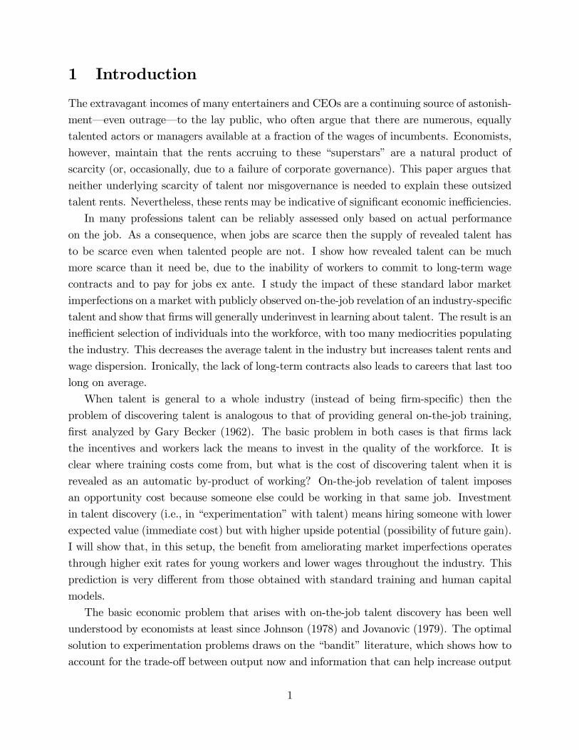
1 Introduction
The extravagant incomes of many entertainers and CEOs are a continuing source of astonish-
ment� even outrage� to the lay public, who often argue that there are numerous, equally
talented actors or managers available at a fraction of the wages of incumbents. Economists,
however, maintain that the rents accruing to these �superstars� are a natural product of
scarcity (or, occasionally, due to a failure of corporate governance). This paper argues that
neither underlying scarcity of talent nor misgovernance is needed to explain these outsized
talent rents. Nevertheless, these rents may be indicative of signi�cant economic ine¢ ciencies.
In many professions talent can be reliably assessed only based on actual performance
on the job. As a consequence, when jobs are scarce then the supply of revealed talent has
to be scarce even when talented people are not. I show how revealed talent can be much
more scarce than it need be, due to the inability of workers to commit to long-term wage
contracts and to pay for jobs ex ante. I study the impact of these standard labor market
imperfections on a market with publicly observed on-the-job revelation of an industry-speci�c
talent and show that �rms will generally underinvest in learning about talent. The result is an
ine¢ cient selection of individuals into the workforce, with too many mediocrities populating
the industry. This decreases the average talent in the industry but increases talent rents and
wage dispersion. Ironically, the lack of long-term contracts also leads to careers that last too
long on average.
When talent is general to a whole industry (instead of being �rm-speci�c) then the
problem of discovering talent is analogous to that of providing general on-the-job training,
�rst analyzed by Gary Becker (1962). The basic problem in both cases is that �rms lack
the incentives and workers lack the means to invest in the quality of the workforce. It is
clear where training costs come from, but what is the cost of discovering talent when it is
revealed as an automatic by-product of working? On-the-job revelation of talent imposes
an opportunity cost because someone else could be working in that same job. Investment
in talent discovery (i.e., in �experimentation�with talent) means hiring someone with lower
expected value (immediate cost) but with higher upside potential (possibility of future gain).
I will show that, in this setup, the bene�t from ameliorating market imperfections operates
through higher exit rates for young workers and lower wages throughout the industry. This
prediction is very di¤erent from those obtained with standard training and human capital
models.
The basic economic problem that arises with on-the-job talent discovery has been well
understood by economists at least since Johnson (1978) and Jovanovic (1979). The optimal
solution to experimentation problems draws on the �bandit�literature, which shows how to
account for the trade-o¤ between output now and information that can help increase output
1
in the future.1 There are many papers that combine experimentation in a labor market
with further features, for example, with multiple job types in MacDonald (1982) and Miller
(1984), and with superstar economics in MacDonald (1988). Common to all these papers
is that young workers absorb the full cost of learning. Realistically, market imperfections
prevent young workers from paying up-front the full price of jobs that require signi�cant
resources. When individuals can not commit to long-term wage contracts then the value of
information accrues as rents to those who turn out to be high talents and see their wages bid
up, so �rms ignore the option value of previously untried individuals. As a direct consequence
of diminished experimentation, there is an ine¢ ciently low level of exit of workers from the
industry. If talent is revealed relatively quickly, then most of the active workforce may consist
of �mediocre�types who would exit the industry in the e¢ cient solution.
If individuals were able to buy their jobs then inexperienced individuals would pay for
the chance to �nd out their talent, up to the expected value of lifetime talent rents. Entering
workers would in e¤ect �buy out�the mediocrities by compensating their employers for the
di¤erence in expected output. This would lead to the e¢ cient solution, where relatively high
talents exit the industry when their jobs have higher social value in trying to discover even
higher talent. I show that if there is signi�cant uncertainty over talent then the e¢ cient
buy-out price for jobs includes most of the complementary costs of production. The e¢ cient
starting wage can therefore be signi�cantly negative, and a small ability to pay for jobs is
therefore of limited help for e¢ ciency as it only buys out few of the mediocre incumbents.
I use a simple one-shot learning process in order to study the market-level implications
of constraints on individual liquidity and commitment ability. I assume ex ante identical
individuals and �nite lifespans, and a competitive industry that faces a downward-sloping
demand curve for its total output. Some �rms must hire new workers in any stationary
equilibrium or else the industry disappears, so the price of output must adjust to allow
for novice-hiring �rms to break even. To highlight the source of the ine¢ ciency, several
commonly studied features of labor markets are ignored in this paper. There is no on-the-
job training or learning-by-doing, so experience per se is not economically valuable. There
are not any frictions such as hiring, �ring, or search costs. Information is symmetric at all
times: There are no e¤ort problems, career concerns, or adverse selection. There is never a
question of e¢ ciency given the available workforce� the economic problem is the selection
of individuals into the workforce.
This paper provides an explanation for extremely high wages in many industries that
appear to be based on talent rents. This explanation is distinct from, and complementary
to, theories based on scale e¤ects (see, e.g., Mayer 1960 and Lucas 1978), superstar eco-
nomics (Rosen 1981), and complementarities in matching (Kremer 1993). These theories are
1See Gittins (1989) for a general treatment of experimentation problems.
2
concerned with the e¢ cient allocation of capital, consumers, and known talent, whereas the
focus here is on the discovery process of talent under typical labor market imperfections. The
previous explanations can still leave one to wonder, for example, why some alternative man-
ager would not be equally good as the current CEO with his exorbitant compensation, scale
e¤ects and complementarities notwithstanding. Intriguingly, industries with the highest and
most skewed pay levels� entertainment and top management� tend to have largely publicly
observable performance.2 The model suggests that this observability may be a key cause of
high pay, and that �erce bidding for known top talent could indicate dramatic ine¢ ciencies
in the selection of individuals into these industries.
The empirical content of the model is in predictions about how a labor market with public
learning would react to changes in individual commitment ability and liquidity. However, the
model does not generate novel wage dynamics, so the ine¢ ciencies cannot be detected even
from the best wage data if the institutional setup remains constant.3 Empirical detection
of the excess talent rents and the welfare loss from ine¢ cient hiring requires a particular
natural experiment.
The plan of the paper is as follows. Section 2 presents the basic model. In Section 3 the
model is used to analyze the equilibrium impact of a worker liquidity constraint on e¢ ciency,
wages, and turnover. Section 4 discusses the implications and the limitations of the model.
Sections 5 and 6 analyzes two alternative speci�cations, where workers are risk averse and
talent de�nes quality instead of quantity of output. Section 7 relates the predictions of the
model to three potential empirical applications from the entertainment industry, and Section
8 concludes.
2 The Model
2.1 Assumptions
Consider an industry where any �rm can combine one worker with other inputs at a cost c > 0
per period. The resulting output is equal to the worker�s talent, �. There is an unlimited
supply of potential workers who face an outside wage w0 � 0. Talent is drawn from a
distribution with a continuous and strictly increasing cumulative distribution function, F ,
with positive support [�min; �max]. The talent of a novice worker is unknown, including to
himself. Talent is industry-speci�c and becomes public knowledge after one period of work;
the worker may then work in the industry up to T more periods, after which he ceases to be
2Observability does not require knowing how they did it but merely how successfully they did it.3Due to the absence of long-term contracts, wage growth merely re�ects the change in the expected output
based on observed performance. For more general models that focus on wage dynamics under symmetric
learning see Harris and Holmström (1982), Farber and Gibbons (1996), or Gibbons and Waldman (1999).
3

productive. Both workers and �rms are risk neutral and there is no discounting.
Firms are potentially in�nitely lived and maximize average per-period pro�ts. Industry
output faces a downward-sloping demand curve pd (q). The number of �rms is �large� so
that individual �rms have no impact on total output and there is no uncertainty about the
realization of the distribution of talent. The matching of individuals and �rms is inconse-
quential. Hence, for simplicity, let the number of �rms (and jobs) be a continuous variable,
I, equal to the mass of the industry workforce. Finally, long-term wage contracts are not
enforceable because workers cannot commit to decline higher o¤ers from other �rms in the
future.
2.2 Average Talent
In both market equilibrium and in the social planner�s optimal solution individual careers
will proceed in a simple manner: After one period of work, those whose talent is revealed
to be below a certain threshold level exit the industry, while those above the threshold stay
on for T more periods. This exit threshold will be the key variable in the model.4 As a
preliminary step, I now derive the steady-state relation of the exit threshold, , and the
average talent of workers in the industry, A.
The vacancies left by last period�s novices who did not make the grade and by retiring
veterans must be �lled by a new cohort of novices. Denote the fraction of novices in the
workforce by i; a fraction F ( ) of them exit. The remaining fraction of jobs 1� i are held
by veterans; a fraction 1=T of these, the oldest cohort, retires each period. Equating the
�ows of exit and entry yields
iF ( ) +1
T(1� i) = i =)
i( ) =1
1 + T (1� F ( )).(1)
The expression i( ) also measures the turnover in and out of the industry (as a fraction of
the industry workforce) because all new entrants are of the youngest type. Its reciprocal
gives the average length of careers in the industry.
The average talent of workers in the industry is
(2) A( ) � i( )�� + (1� i( ))E[�j� � ].
Substituting the fraction of novices from (1) into (2) shows that average talent is
(3) A( ) =1
1 + T (1� F ( ))�� +
T (1� F ( ))
1 + T (1� F ( ))E[�j� � ].
4The selection of types must be based on a single threshold whether there is a welfare-maximizing social
planner or a market equilibrium: If some veteran type �0 stays in the industry then all types � > �0 will also
stay, because all veterans have the same opportunity cost regardless of age or type.
4

2.3 Social Planner�s Problem
Consider the problem of maximizing social surplus by choosing the exit threshold and
employment I. Social surplus consists of total bene�t to consumers minus the opportunity
costs of production
(4) S(I; ) =
Z IA( )
0
pd(q)dq � I (w0 + c) .
It is apparent that, for any given choice of I, the exit threshold should be chosen to maximize
the average level of talent A.
To maximize the average talent (3), take the �rst-order condition:
@
@ A( ) =
T f( )
(1 + T (1� F ( )))2��� + T (1� F ( ))E[�j� � ]
� T f( )
1 + T (1� F ( ))= 0
=) �� + T (1� F ( ))E[�j� > ] � (1 + T (1� F ( ))) = 0.(5)
This can be rearranged to yield a more useful condition:
(6) � �� = T (1� F ( )) (E[�j� � ]� ) .
Denote the solution to (6) henceforth by A�. (It will soon be shown to be unique).
It is useful to understand the economic intuition behind (6). The hiring of a novice
instead of a veteran of above-average talent can be interpreted as an investment. The LHS
gives the cost � the immediate loss in expected output from hiring a novice instead of
the threshold veteran. The RHS shows the expected future gain, assuming that the same
rehiring threshold is still used in the future. The trade-o¤ is that a higher threshold results
in higher-quality veterans, but also in a larger fraction of the workforce being novices. The
lowest talent to be retained is the marginal talent in the workforce, and, as usual, the average
is maximized when it equals the marginal. Therefore the optimal exit threshold is also the
maximum attainable average level of talent in the industry: A� = A(A�).5
Uniqueness of A� requires no further assumptions about the shape of the talent distrib-
ution.
Lemma 1 The maximized average level of talent is equal to the optimal exit threshold, thisthreshold is unique and above the population mean.
5With discounting, the maximizer would be below the maximum: a lower exit threshold amounts to a
lower level of investment.
5

Proof. To see that the solution to (6) is a �xed point of A, �rst solve for the (linear)
term and then divide both sides by 1 + T (1� F ( )). This shows that is equal to the
objective function A, from (3), evaluated at . To see uniqueness, note that the LHS of
(6) is strictly increasing� it has slope equal to one� and the RHS is decreasing� with slope
equal to �T (1� F ( )). The LHS is equal to zero at = ��, while the RHS is equal to
T (�� � �min)> 0 at = �min and reaches zero at = �max. Thus the unique solution to (6)
is in (��; �max).�Finally, employment I should be set to equate total output with demand at the minimized
average cost, so that pd(IA�) = (w0+ c)=A�. Note that the industry as a whole has constant
returns to scale: To double the output, the amount of novices hired and total costs would
both be doubled; this would double the amount of veterans as well.
3 Equilibrium Analysis
3.1 Equilibrium Conditions
I only consider the steady state. (I will later show that there is only one steady state
equilibrium; Appendix A proves, for T = 1, that all market equilibria converge to the steady
state.) In steady state all aggregate variables are constant over time, although individuals
and their fortunes vary over time. The wage function w (�), output price P , and employment
I, must be consistent with the following four conditions.
First, �rms must expect zero pro�ts from hiring any talent, so
(7) P� � c� w (�) = 0
for all �. Information is symmetric, so �rms view novices as equivalent to workers with a
known talent equal to the population mean ��. (The notation will exploit this and treat
novices simply as ��-types.)
Second, as veterans have no upside potential, they exit if w (�) < w0. Due to the con-
tinuum of types, the lowest type veteran worker, , must be indi¤erent between exiting and
staying and thus earns exactly the outside wage:
(8) w( ) = w0.
Third, novices must be indi¤erent between entering the industry or the outside career,
taking into account the option to exit for the outside career later on:
(9-A) w����+ TE[max fw (�) ; w0g] = (1 + T )w0.
Individual careers consist essentially of two periods, and T is the relative length of the veteran
period. Condition (9-A) assumes that novices are �nancially unconstrained: Depending on
6

parameters, this can mean accepting a negative wage. This e¢ cient benchmark will be
compared to the case of constrained individuals, where novices can not accept a wage lower
than w0�b, where b is an exogenous ability to �pay�for a job. When b is a binding constraintthen (9-A) is replaced by
(9-B) w����= w0 � b.
Finally, output price must be consistent with the demand for industry output:
(10) P = pd (IA ( )) ,
where average talent A ( ) gives the average output per worker in the industry.
In labor market equilibrium, expected di¤erences in talent must be consistent with corre-
sponding di¤erences in wages. It turns out that the equilibrium wage function can be de�ned
conditional on the equilibrium exit threshold . This insight will later simplify the analysis
of �nancial constraints, as their impact can be captured by the distortion on . Denote the
equilibrium wage function conditional on the exit threshold by w(�j ).
Lemma 2 Given an equilibrium exit threshold , the price of output is P ( ) = (w0 + c) =
and wages are
(11) w(�j ) = (w0 + c)
��
� 1�+ w0.
Proof. A �rm employing a threshold type gets revenue P and has costs w( j )+ c =w0 + c. For expected pro�ts to be zero, the equilibrium price must make these be equal,
so P ( ) = (w0 + c) = . For �rms to be indi¤erent between and any other talent, the
di¤erence in wages must just o¤set the di¤erence in revenue generated, so w(�j )�w( j ) =P ( ) (� � ): Combining this with the equilibrium price and w( j ) = w0 yields equation
(11).�
3.2 Unconstrained Individuals
Competitive equilibrium with unconstrained individuals is socially e¢ cient, so the social
planner�s solution already tells us that the exit threshold must be = A� > ��. Looking
back at the wage equation (11), it is clear that novices must accept less than the outside
wage w0. After all, they have a positive probability of earning talent rents in the future
while in the worst case they get the outside wage. Market equilibrium pins down the wage
function from Lemma 2 as w(�jA�) and the price of output as P � = (w0 + c) =A�.
Intuitively, note that unconstrained individuals bid for the chance to enter the industry
up to the expected value of lifetime talent rents. As veterans of threshold type are available
7
at the outside wage, novices have to pay P � ( � ��) for their �rst period job: This paymentexactly compensates a novice-hiring �rm for its expected revenue loss (compared to what
it would get by hiring a threshold type). In equilibrium, this novice payment must equal
the expected lifetime rents: With threshold , a novice has a probability 1� F ( ) of being
retained, in which case he gets the excess revenue P � (� � ) as a rent on each of the T
remaining periods of his career. This equality is the market equilibrium condition
(12) P � ( � ��) = (1� F ( ))TP � (E[�j� � ]� ) .
The price of output P cancels out of the equilibrium condition, which reduces to the �rst-
order condition (6) of the social planner�s problem and thus yields A� as the solution. Unique-
ness follows from Lemma 1. Payments by unconstrained novices raise the exit threshold to
the e¢ cient level. As is typical, the inability of workers to commit to long-term contracts
does not cause problems when they are able to buy their jobs up-front.
The unconstrained payment (the price of a job) re�ects the economic cost of the e¢ cient
level of experimentation. It is
(13) b� � P ��A� � ��
�= (w0 + c)
�1�
��
A�
�.
The fraction of the total costs of production, w0 + c, that should be �nanced by the novice
is increasing in A�=��, which is a measure of the upside potential of novices. For small values
of b� the novice payment would merely be a wage discount below the outside wage.
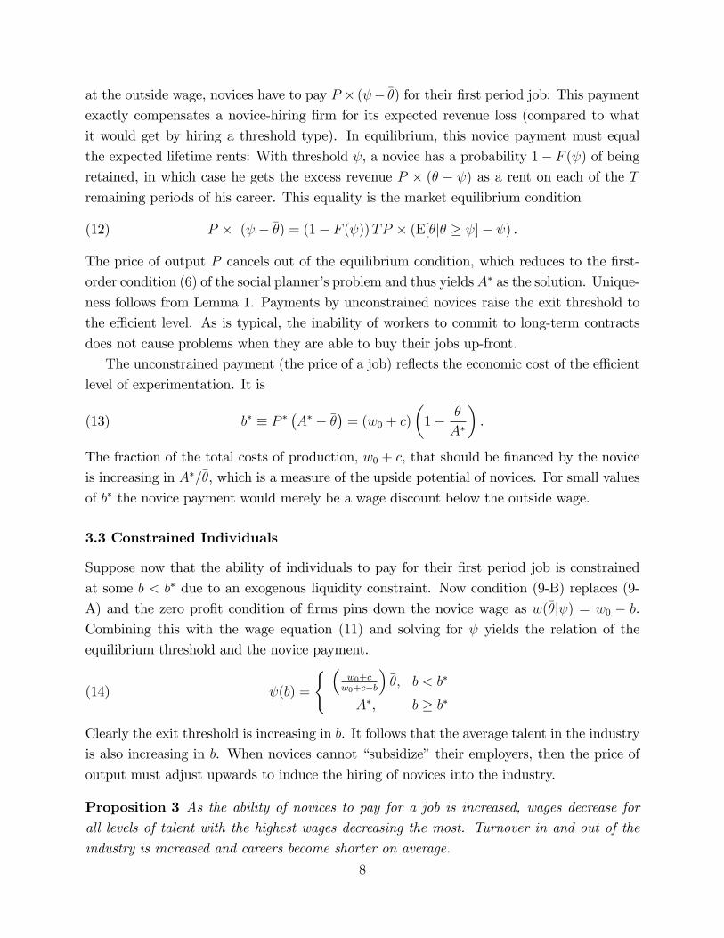
3.3 Constrained Individuals
Suppose now that the ability of individuals to pay for their �rst period job is constrained
at some b < b� due to an exogenous liquidity constraint. Now condition (9-B) replaces (9-
A) and the zero pro�t condition of �rms pins down the novice wage as w(��j ) = w0 � b.
Combining this with the wage equation (11) and solving for yields the relation of the
equilibrium threshold and the novice payment.
(14) (b) =
( �w0+cw0+c�b
���; b < b�
A�, b � b�
Clearly the exit threshold is increasing in b. It follows that the average talent in the industry
is also increasing in b. When novices cannot �subsidize�their employers, then the price of
output must adjust upwards to induce the hiring of novices into the industry.
Proposition 3 As the ability of novices to pay for a job is increased, wages decrease forall levels of talent with the highest wages decreasing the most. Turnover in and out of the
industry is increased and careers become shorter on average.
8
Proof. First, using Lemma 2, note that @@ w(�j ) = � (w0 + c) �= 2 and @2
@�@ w(�j ) =
� (w0 + c) = 2; both negative. Second, from equation (14) we get 0(b) > 0 for b < b�.
The e¤ects on wages follow from combining these. Direct inspection of (1) reveals that
i ( ) is increasing, so the e¤ects on turnover i ( ) and average career length 1=i ( ) follow
immediately from the higher .�
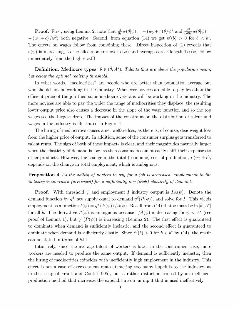
De�nition. Mediocre types: � 2 (��; A�). Talents that are above the population mean,but below the optimal rehiring threshold.
In other words, �mediocrities� are people who are better than population average but
who should not be working in the industry. Whenever novices are able to pay less than the
e¢ cient price of the job then some mediocre veterans will be working in the industry. The
more novices are able to pay the wider the range of mediocrities they displace; the resulting
lower output price also causes a decrease in the slope of the wage function and so the top
wages see the biggest drop. The impact of the constraint on the distribution of talent and
wages in the industry is illustrated in Figure 1.
The hiring of mediocrities causes a net welfare loss, as there is, of course, deadweight loss
from the higher price of output. In addition, some of the consumer surplus gets transferred to
talent rents. The sign of both of these impacts is clear, and their magnitudes naturally larger
when the elasticity of demand is low, as then consumers cannot easily shift their expenses to
other products. However, the change in the total (economic) cost of production, I (w0 + c),
depends on the change in total employment, which is ambiguous.
Proposition 4 As the ability of novices to pay for a job is decreased, employment in theindustry is increased (decreased) for a su¢ ciently low (high) elasticity of demand.
Proof. With threshold and employment I industry output is IA( ). Denote the
demand function by qd, set supply equal to demand qd(P ( )), and solve for I. This yields
employment as a function I( ) = qd (P ( )) =A( ). Recall from (14) that must be in [��; A�]
for all b. The derivative I 0( ) is ambiguous because 1=A( ) is decreasing for < A� (see
proof of Lemma 1), but qd (P ( )) is increasing (Lemma 2). The �rst e¤ect is guaranteed
to dominate when demand is su¢ ciently inelastic, and the second e¤ect is guaranteed to
dominate when demand is su¢ ciently elastic. Since 0(b) > 0 for b < b� by (14), the result
can be stated in terms of b.�Intuitively, since the average talent of workers is lower in the constrained case, more
workers are needed to produce the same output. If demand is su¢ ciently inelastic, then
the hiring of mediocrities coincides with ine¢ ciently high employment in the industry. This
e¤ect is not a case of excess talent rents attracting too many hopefuls to the industry, as
in the setup of Frank and Cook (1995), but a rather distortion caused by an ine¢ cient
production method that increases the expenditure on an input that is used ine¤ectively.
9

3.4 Long-Term Wage Contracts
Under short-term contracts, the extent to which the upside potential of novices is taken into
account depends solely on how much novices can pay for jobs. Worker ability to commit to
long-term wage contracts would give another incentive for �rms to hire novices over mediocre
veterans: Firms would get a share of the rents to high talents as these would be forced to
stay at the discovering �rm at the original contract wage.6
Suppose now that novices can commit to a long-term wage contract, meaning that they
can promise to work for their initial employer for 1+ S periods at some agreed wage. Firms
can still �re workers after one period. For simplicity, let�s also assume that b = 0. Firms
can attract novices by o¤ering a contract that matches the outside opportunity of constant
wage at w0. In case the worker doesn�t make the grade, he will be �red and earns the w0outside the industry. How does the �rms�retaining threshold depend on S?
A �rm that uses a retaining threshold and keeps the retained workers for S more periods
has a long-run average talent level as given by equation (3), but with the commitment time
S replacing T . Let�s denote this average by A( jS). The long-run average pro�ts are
PA( jS) � w0 � c; to maximize this a novice-hiring �rm will choose a rehiring policy that
maximizes A( jS). As nothing has changed from the social planner�s maximization conditionexcept the length of retainment, the solution to equation (6)� with S replacing T� gives the
�rms�optimal rehiring policy. Let�s denote it by �(S).
As for the free agents, i.e., workers who have served the full 1 + S periods, they stay in
the industry until retirement. Other �rms compete for them, bidding up their wages until
�rms make zero pro�ts and talent rents accrue to the free agents. The wage equation (11)
must thus hold for the free agents, so their wages are given by w(�j �(S)). No �rm will hireworkers discarded by another �rm after one period� after all, they could achieve a higher
average talent level at the same wage by becoming a novice-hiring �rm themselves.
Proposition 5 As the length of time for which workers can commit to a wage contract isincreased, the wages of free agents decrease for all levels of talent with the highest wages
decreasing the most. Turnover is increased and careers become shorter on average.
Proof. First, totally di¤erentiate equation (6) with respect to and T , where T nowstands for the contract length, and apply the envelope theorem. This yields
(15)@ �(T )
@T=
1� F ( )
1 + T (1� F ( ))fE[�j� � ]� g > 0.
The e¤ects of the increased threshold on wages, turnover, and career length follow as in the
proof of Proposition 3.�6As before, this analysis assumes that the industry is in steady state.
10
Commitment to long-term contracts can be regarded as a type of a payment from workers
to employers. Any commitment time beyond what it takes to reveal talent gives �rms some
talent rents and induces them to replace the worst mediocrities with novices instead of the
lowest types of mediocrities. The longer the duration of commitment, the closer the solution
is to full e¢ ciency and the lower the wages of free agents of any given talent. Full e¢ ciency
is achieved only if novices can commit to a wage contract for the full length of the career.7
4 Discussion
To summarize, the main e¤ect of the constraints on individual ability to pay for jobs and
to commit to long-term wage contracts is that the standard of performance required for a
worker to be retained in the industry is too low. The proportion of inexperienced workers
and the average level of talent in the industry are both ine¢ ciently low. Just as a matter
of accounting, this implies that careers are too long on average. Furthermore, the ine¢ cient
selection of workers increases talent rents in two ways. First, rents accrue to the di¤erence
in units of output that an individual makes compared to the threshold type; this di¤erence
is higher for any retained type when the threshold is lower. (This is the standard Ricardian
component of talent rents.) Second, the value of this advantage is increasing in the price
of output, which is higher in the constrained case because the equilibrium price must allow
novice-hiring �rms to break even.
When is the hiring of mediocrities likely to be economically signi�cant, in terms of the
welfare loss and the excess rents to talent? Ine¢ ciencies are increasing in the discrepancy
between the social value of experimentation, b�, and what novice workers are able to pay
for a job. There are two features that increase b�: the costs of production per job and the
upside potential of novices. This can be seen from (13) where b� is a product of these two
factors.
Consider �rst the costs of production, w0 + c. When jobs require few inputs� as in the
case of a street performer� then the production cost is mostly just the opportunity cost of
the individual�s own labor, and the novice wage is easily be positive and liquidity constraints
are unlikely to cause problems. In this way the role of c is analogous to that of a training
cost in a traditional human capital setup, where the provision of cheap training is not a
problem because a modest wage discount will pay for it. However, when jobs are expensive,
for example due to expensive equipment, then c could be orders of magnitude beyond the
7In practice, even career-long contracts would be unlikely to achieve full e¢ ciency, since the ability to
perform at the full talent level is inherently unveri�able and any renegotiation ability by workers would
reduce the incentives to hire novices. For an analysis of renegotiation of labor contracts, see e.g., Aghion,
Dewatripont and Rey (1994) or Malcomson (1997).
11

reasonable ability of novices to pay for. The production cost does not merely apply to inputs
that the worker is physically handling, but to any costs within the �rm that are necessary
for the job to be real in the sense that the talent gets revealed. For example, for a manager,
the entire wage bill of her subordinates could be part of the production cost, if the talent in
question is for managing a large organization.
The other factor in b�, the upside potential of novices 1 � ��=A�, measures the shortfallof expected novice output relative to the e¢ cient threshold level (which is also the maxi-
mized workforce average talent). This shortfall is precisely the fraction of production costs
that novices have to �nance in the unconstrained case. Note that it is a purely �statistical�
property of the distribution of talent and T . However, in a liquidity constrained world, an
increase in the cost c results in a lower exit threshold.8 We saw already that A�, and there-
fore the shortfall, is increasing in T , as it is e¢ cient to have tougher retainment standards
when those retained can be kept for longer (equivalently, when talent is revealed relatively
quickly).9 Furthermore, the shortfall is higher when there is wide dispersion in the right
tail of the talent distribution. Intuitively, the more right-skewed the distribution, the higher
the upside potential that novices have and the higher the burden of �nancing they should
bear. The e¤ect of skewness can be explored succinctly by assuming that talents are drawn
from the Weibull distribution, which has the feature that skewness is decreasing in the shape
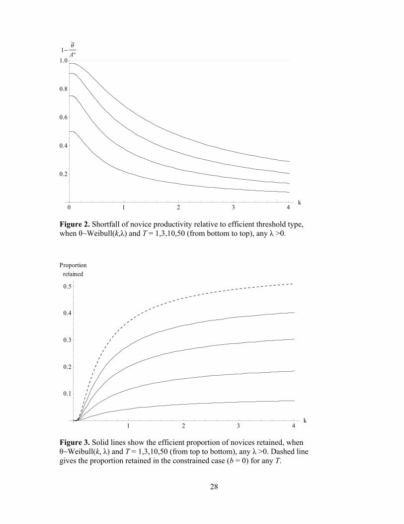
parameter.10 Figure 2 graphs the shortfall ratio for various values of T as a function of the
Weibull shape parameter. It shows that novices could easily have to �nance a signi�cant
fraction (even most) of the production costs. Figure 3 shows the associated retainment prob-
abilities. For more right-skewed distributions a smaller proportion of novices is retained; in
the limit the proportion retained becomes arbitrarily small.
Additional market imperfections could partially alleviate the problem of ine¢ cient hiring,
in typical second-best fashion. For example, market power by �rms in the labor market would
encourage experimentation as it would allow �rms to capture some of the returns. The
mechanism would be the same as in the general training setup where imperfect competition
(see, e.g., Acemoglu and Pischke 1999a, 1999b) and asymmetric information (Greenwald
1986, Katz and Ziderman 1990) induce �rms to invest into general training. A collusive
industry could also set up mitigating institutions, such as minor leagues in team sports where
talent can be revealed in a cheaper way (but probably less accurately) . However, market
8Higher outside wage w0 also decreases the threshold, but this is holding constant novice liquidity b which
would in many cases bear some relation to w0.9On the other hand, for very quick revelation of talent the unconstrained novice payment gets smaller as
a fraction of lifetime wages so borrowing constraints would likely be less of a problem.10The Weibull CDF is F (�) = 1 � e�(
�� )
k
. (Here the scale parameter can be normalized � = 1 without
loss of generality.) The distribution is Exponential at k = 1 and approximates the Normal distribution near
k = 3:5, above which skewness is negative.
12

power in the labor market is likely to coexist with some market power in the product market.
In a clear-cut extreme case the whole industry would be a single �rm, i.e., a monopolist in
the product market and a monopsonist in the labor market. Such a �rm would minimize
its costs by enforcing the socially optimal exit threshold. The monopolist would face a
lower marginal cost than �rms in a competitive industry, but it would also mark up the
output price. The monopolist is thus better for welfare than perfect competition if demand
is su¢ ciently elastic.11
4.1 Limitations of the Model
To keep the model simple it did not explicitly treat the dissipation of rents. Realistically,
individuals entering careers where the scarcity of talent is due to the scarcity of opportuni-
ties for revealing talent should not earn expected rents over their lifetimes. However, rent
dissipation does not imply that novices should earn zero wages (although some starving
artists certainly do), only that the expected lifetime utility is equal across alternative careers
pursued by ex-ante similar individuals. For workers with comfortable outside opportunities,
the wage that is low enough to dissipate the expected lifetime rents from a career that in-
volves a longshot at stardom can still be considerable, simply due to diminishing marginal
utility. Some of the expected rents are lost (in the welfare sense) by having workers bear the
risk in their uncertain success. Painfully high e¤ort is another way in which any amount of
rents can be dissipated with little increase in the monetary payment for jobs. In the movie
industry, some talent rents are surely dissipated in the queuing for entry-level positions, by
forgoing education or job experience in other sectors, and perhaps on the casting couch.
Carmichael (1985) has shown that, in e¢ ciency wage models,12 arbitrarily small entrance
fees eliminate involuntary unemployment as long as they lower the new hires�utility to the
level of their outside utility. Here entrance fees are useful only to the extent that they �buy
out�incumbent workers from their jobs. In professions with signi�cant production costs and
a right-skewed distribution of talent, small payments can only displace a small segment of
the mediocrities, no matter how much novice utility they dissipate.
The assumption that novices are ex-ante identical is a simpli�ed representation of the
fact that the dispersion of prior expected values of talent is small compared to the actual
dispersion of talent. A model where novices are heterogeneous by expected talent requires
two thresholds and two distributions� one for novices and another for veterans� and results
in expected talent rents for the inframarginal novices but yields no additional insights. The
11For example, with a constant elasticity of demand � < �1 and b = 0 the competitive output price is
(w0 + c)=�� while the marginal cost for a monopolist is (w0 + c)=A�. A monopolist marks up its price by a
factor �= (1 + �) and so is better for consumers if j�j > A�=�A� � ��
�.
12See Shapiro and Stiglitz (1984).
13

e¢ cient policy still requires the marginal veteran to be signi�cantly better than the marginal
novice. Under liquidity constraints the novice threshold is too high and the veteran threshold
too low, and the two thresholds coincide at the extreme case b = 0.
In many industries talent is revealed in successive tiers of ever more demanding tasks.
The ine¢ cient selection of workers can also apply to such careers, for example where higher
tiers mean managing larger and more complex organizations. Success as a low-level manager
gives a noisy signal about the ability to be a higher-level manager, but those who succeed
as low-level managers cannot all be tried out at the next level of hierarchy. Each level of
promotion creates a bottleneck of talent discovery akin to the one-task model, but with
heterogeneous novices (by expected talent). The relevant complementary cost in jobs where
managerial talent can be uncovered includes the cost of capital under management and the
wages of subordinates, so the experimentation cost and the problem of mediocre hires and
excess rents would tend to get worse higher up in the hierarchy.
The one-shot learning process is a key simpli�cation to keep the model tractable. A sepa-
rate appendix13 shows that the main results of the basic model have analogous counterparts
in a setup where information about talent is revealed gradually over time. There the de�ni-
tion of the optimal exit threshold is more complex as the option to exit in the future must
also be taken into account. In the absence of a liquidity constraint, the decision to exit for
the safe outside wage is analogous to the optimal stopping policy in Jovanovic (1979), while
under constrained liquidity the individually optimal stopping policy is ine¢ ciently lenient.
The additional insight brought by gradual learning is that saving by incumbents makes worse
the ine¢ ciency caused by the credit constraint. Saving allows �has-been� individuals who
perform well early in their career but who fall below (but not too far below) population
mean in perceived talent to outbid credit-constrained novices for positions. Their incentive
to pay for positions is a gamble for resurrection: As talent is only revealed over time, even
the has-beens still retain some upside potential, albeit less than the novices.
Even though the product market was assumed to be perfectly competitive, competition
in the labor market is both necessary and su¢ cient for liquidity constraints to result in
ine¢ cient hiring. The crucial e¤ect coming from the �rm side is that competition between
employers turns the discovery of new talent into a public good problem within the industry.
If the price of output price were a �xed parameter (e.g., due to an exogenously �xed num-
ber of jobs and in�nitely elastic demand) then the excess talent rents caused by a novice
liquidity constraint would have to come at the expense of �rms�pro�ts (instead of consumer
surplus). The model would then have to assume su¢ ciently large economic pro�ts to �rms
in the unconstrained case, or else the constrained case results in the boring equilibrium of no
production at all as �rms couldn�t break even at the �xed output price. A model with a com-
13Available from http://faculty.haas.berkeley.edu/marko/MediocritiesAndSuperstars_GradualLearning.pdf.
14
petitive product market is thus more parsimonious and, arguably for long-run equilibrium,
also a more realistic assumption than a �xed price of output.
5 Risk Averse Individuals
The exogenous borrowing constraint of the basic model is merely a simplifying assumption.
The analytical convenience of linear utility is that it allows for tractable closed-form solu-
tions. However, if individuals are risk averse then similar results obtain even if they have
unlimited ability to borrow or su¢ cient endowments to pay for their �rst job. In this case the
exogenous liquidity constraint is replaced by an endogenous constraint: The wage discount
that risk averse novices are willing to accept is less than b� in (13). The ine¢ ciency can
be interpreted as a problem of incomplete markets, as individuals cannot perfectly hedge
against the realization of their own initially unknown talent level.14
To brie�y explore the risk averse case, assume now that individuals have some concave
utility function u (but are still ex ante identical). The di¤erence between the outside wage
and the novice wage can be interpreted as the price of an option to future talent rents; the
option value comes from the possibility to exit and switch to the outside wage if talent turns
out to be low. This option must have a positive price in equilibrium. However, risk averse
novices are willing to pay less than the risk neutral value of this option. This leads to the
same ine¢ ciencies as the exogenously assumed liquidity constraint of the basic model.
Proposition 6 Equilibrium exit threshold is decreasing and wages for all talent levels are
increasing in individual risk aversion.
Proof. The exit threshold that results in equilibrium wages that keeps expected
lifetime utility equal with the utility from the outside career must satisfy
(16) w0 � w���j �= T CEu[max fw (�j ) ; w0g]� Tw0,
where CEu is the Certainty Equivalent operator. Veterans stay in if w (�j )�w0 > 0, whichstill pins down the relation of output price and exit threshold as P ( ) = (w0+c)= . Lemma
2 applies, and (16) can be written as
(17) (w0 + c)
�1�
��
�= TCEu
�max
�(w0 + c)
��
� 1�, 0�+ w0
�� Tw0.
The left-hand side of (17) is zero at = �� and increasing in . The right-hand side is strictly
positive at = �� and decreasing in , but goes to zero as reaches �max (as the option
14Figure 2 shows the magnitude of the downside risk: The entry payment is wasted with the probability
that novices are not retained.
15

will then never be exercised). Thus there is a unique equilibrium u 2 (��; �max). In thespecial case of risk neutral individuals, CEu is just the expected value, and (17) reduces to
(6), thus leading to the socially e¢ cient solution. Compared to the risk neutral case, only
the right-hand side of (17) changes, shifting down (because CE is always below Expected
Value), so u must be lower than in the risk neutral case to restore the equality. By the same
argument, and by the standard de�nition of comparisons in risk aversion, u is decreasing in
risk aversion and reaches �� in the limit of in�nite risk aversion. The impact on wages follows
from (11).�
6 Talent as Quality
In most markets talent is more naturally associated with the quality rather than the quantity
of output. In this section the model is generalized to a case where talent is de�ned as the
quality of output. The purpose is to show that the results are robust and, secondarily, to
make a connection with the classic superstar model of Rosen (1981). To follow Rosen�s setup,
here producers choose their level of output, taking as given the unit price that it commands
in the market. Due to consumer preferences, higher quality output faces a higher unit price
so, in addition to standard Ricardian rents, the higher talents gain a further advantage by
�nding it optimal to produce more output than the lesser talents. Rosen found that this
can cause modest di¤erences in talent to result in vast di¤erences in income, with a small
number of top talents serving most of the market.15
On the consumer side, the di¤erence to the basic model is that demand is assumed to come
from a mass of identical consumers with quasilinear utility u (x)+q�, where q is the quantity
and � the quality of the good, and x is the composite of all other goods used as the numeraire.
Consumers face budget constraint M = x + p (�) q, where M is the exogenous income and
p (�) the endogenous unit price of a good with quality �. Di¤erentiating u (M � p (�) q)+ q�
with respect to � and q yields the �rst-order conditions of consumers choice, which can be
combined to the indi¤erence condition
(18) p0 (�) =p (�)
�.
Integration yields the �price-talent indi¤erence curve,�
(19) p(�) = P�;
where P is now �the implicit market price�(Rosen�s terms in quotes), arising as the constant
of integration from (18). In equilibrium, consumers must be indi¤erent between all quality
15This section also draws on MacDonald (1988) which combined Rosen�s superstar setup with public
learning about a binary talent.
16

levels that are on o¤er.16 The quasi-linear utility simpli�es away the issue of consumer
risk aversion with respect to uncertain novice quality: Consumers are willing to pay for
the expected quality. This is reasonable when the good in question takes up a small part
of consumer expenditure. As it will turn out, some quality levels will not be produced in
equilibrium, but this does not a¤ect (19) which must also hold for novices at � = ��.
On the producer side, the di¤erence to the basic model is that �rms control their level
of output s; doing so they face marginal cost � and �xed cost c. Firm with a worker of
talent � faces price P� per unit of its output. Free entry of �rms and the competitive labor
market result in maximized pro�ts being driven to zero, so the earnings of a worker of talent
� conditional on the implicit price P are
(20) ! (�jP ) = maxs�0
�P�s� �
s2
2� c
�=(P�)2
2�� c.
The pro�t-maximizing level of output is s (�) = P�=�. As novice output is produced and
sold before talent is known, (20) holds for them at � = ��.
The impact of a liquidity constraint works similarly as in the basic model. The e¢ cient
exit threshold is higher than the population mean, and novices should compensate �rms that
employ them for the expected di¤erence in the market value of their output compared to
the threshold type. In the constrained case the exit threshold will again be too low, and the
implicit price of talent must adjust to induce �rms to hire novices.
Proposition 7 As the ability of novices to pay for a job is increased, the output and wagesdecrease for all levels of talent, with the highest levels decreasing the most. Turnover in and
out of the industry is increased and careers become shorter on average.
Proof is in Appendix B.To summarize, the basic model is robust to modeling talent as quality. The additional
result is that now the level of output per individual is also distorted in the constrained case:
While workers are less talented on average, each worker type produces more output than
they would in the e¢ cient case.
In Rosen�s superstar setup, technology and consumer preferences result in a nonlinear
relation of talent and revenue. By imposing a linear relation of talent and revenue, the
basic model here highlighted that the classic superstar e¤ect and the market failure in talent
discovery (mediocrity e¤ect) are completely independent mechanisms, although both end up
enhancing the wages of top talents.
16Rosen also included a private �xed cost per quality-level consumed, and discussed (informally) the
implications of further introducing consumer heterogeneity with respect to the �xed cost. It would lead to
consumers having heterogeneous preferences over the quality-quantity tradeo¤ and a single implicit price
would no longer be su¢ cient to capture the equilibrium, rather p(�) would be convex.
17
7 Applications
The prototypical talent markets are found in the entertainment industry. There job perfor-
mance is almost entirely publicly observable and success of young talents hard to predict.
Neither formal education nor on-the-job training seem to play a large role in explaining wage
di¤erences in these industries. The chance to reveal one�s talent in a real job is precious, as
is suggested by the queuing for positions. Auditions seem to have limited usefulness beyond
working as a cut-o¤ that reduces the number of candidates for any entry-level position; huge
uncertainty over talent remains among many viable candidates. There simply is no good
substitute for observing the success of actual end-products. Richard Caves (2000) calls this
uncertainty the �nobody knows�property, as the �rst on a list of distinctive characteristics
of the entertainment industry. It could be argued that �nding out about someone�s talent
in the entertainment industry is more about �nding out the tastes and whims of the pub-
lic than about some objective measure of quality, but this distinction is not economically
meaningful� the economically relevant interpretation of talent is the individual�s ability to
generate revenue.
A suitable natural experiment is needed in order to identify and quantify any ine¢ ciency
caused by the hiring of mediocre incumbents. The most useful experiment would be a
large exogenous change in either the individual liquidity constraint or, more plausibly, in
the length of enforceable wage contracts. The ideal experiment would be a surprise legal
change from individual ability to commit to career-long wage contracts to spot contracting
or vice versa. While empirical analysis of such natural experiments would require further
elaboration, the model presented here can already shed light on stylized facts and suggests
empirical applications. I will next brie�y discuss three potential applications. (For a more
detailed discussion of applications, see the working paper version of this paper).
Motion pictures The motion picture industry in Hollywood operated under the so-
called studio system from 1920s to late 1940s. In this system, artists and other inputs were
assembled together under long-term relationships. New movie actors made exclusive seven-
year contracts with movie studios. This kept the compensation at moderate levels until the
initial seven years came to an end even for those who became stars, allowing studios to
capture much of the value of talent they discovered. The studios could rent artists to other
studios on �loan-outs�but the artists had no right to refuse roles. The contracts did not
provide wage insurance: Even though wages were speci�ed for the whole contract period
the studios retained the right to terminate the contract. At the end of their contracts, the
salaries of the proven stars were bid up by the competing studios. The relatively low initial-
contract wages indicate that pre-contract information about talent was very imperfect and
that unrevealed talent was not scarce.
18

After several court rulings in the 1940s the long-term contracts became practically unen-
forceable and the studio system broke down. According to my model, the end of long-term
contracting should have led to insu¢ cient exit of mediocre entertainers, showing up as higher
and more uneven incomes for veteran actors, and as lower total revenue. The wages of star
actors on their initial contract during the studio system can be expected to be lower for
obvious reasons. More interestingly, the situation of free agents (those past the initial seven
years) under the studio system is comparable to actors with the same amount of experience
under spot contracting, but the end of long-term contracts should have increased their pay,
despite of an accompanying decrease in industry revenue. There is clear evidence of a post-
war decline in revenue and output at movie studios but wage data for actors is lacking.17 An
empirical analysis would require a dynamic model that takes into account how an industry
adjusts from one steady state to another, and how it reacts to demand shocks, such as the
advent of television in the 1950s. (The unusually poor substitutability across age groups�as
most roles must be casted with an actor from a certain age range�may also be a signi�cant
factor). Interestingly, in terms of quality, the era from the 1920s to the 1940s is often referred
to as the golden age of Hollywood movies.
Record Deals Exclusive record deals, by which musicians agree to make a certain
number of albums for the same record company, are a form of long-term wage commitment.
This commitment is enforceable because record deals are not treated as employment contracts
by the courts. The music industry is very competitive at the entry level, where upstart
bands and artists are free agents, but agree to exclusive contracts in exchange of production,
distribution, and promotion by the record company.
Long-term record contracts have always been threatened by the attempts to renege or
renegotiate by artists who turn out to be big stars. Furthermore, there is a recurring lobbying
battle in Congress about the enforcement of multi-record contracts.18 Were the current
system to break down, the proportion of new artists and new releases could be expected to
be reduced, while the proportion of new artists whose record earns pro�ts and who go on
making a second record should go up. Currently about 80-90% of records by new artists
make a loss, so a reduced proportion of �failed artists�would probably be regarded by many
as a sign of a more judicious choice of artists by the record companies, when in fact it would
be a sign of reduced experimentation and lower e¢ ciency.
17According to Caves (2000, p. 389), �no systematic data have been assembled on whether the studios�
disintegration brought more rents into the stars�hands, but casual evidence suggests that it did.�18The protagonists are RIAA (Recording Industry Association of America), representing record companies,
and AFTRA (American Federation of Television and Radio Artists), representing incumbent artists.
19
Professional Team Sports Professional team sports have very unusual labor markets,
mainly because �rms depend on mutual cooperation within leagues that are arguably natural
monopolies. Many leagues have been able to enforce rules that restrict �rms from competing
for each others�employees. Talent in team sports may in part be interpreted as the capability
to bene�t from learning-by-doing, and opportunities to play at the top level are naturally
scarce. Thanks to long-term contracts, clubs have incentives to take into account the upside
potential of their young players instead of just picking the best squad according to current
expectations.
Changes in the duration of contracts can allow ine¢ cient experimentation and excess
rents to talent be measured. Increasing (re)negotiation power by players should lead to
longer careers and higher salaries. There has in fact been variation in the contracting rules
and practices in several team sports. For example, the long-term contracts in American
baseball were for a long time challenged by the players�union which eventually achieved a
six-year cap on the initial contracts. However, this change was by no means a sudden surprise.
(The number of teams and players have also been growing, so the steady-state model is again
not su¢ cient for empirical analysis.) A more drastic experiment may yet begin in European
football, where the EU is considering a complete ban on long-term contracts.19
8 Conclusion
According to Raymond Cotton, a lawyer who specializes in contract negotiations for college
presidents, �what all universities are trying to do is �nd a successor who has been someplace
else as president.�20 The main message of this paper has been that any profession where the
ability of inexperienced workers is subject to much uncertainty, and where performance on
the job is to a large extent publicly observable, is a likely candidate for market failure in the
discovery of talent. This market failure would manifest itself as a bias for hiring mediocre
incumbents at excessive wages. Markets for lawyers, fund managers, advertising copywriters,
and college professors are among other possible cases not explored in this paper. It can be
argued that di¤erences in talent that are only discovered on the job are in fact the main source
of talent rents in the economy. If that is the case, then much of observed superstar incomes
could be, instead of a rent to truly scarce factors, a symptom of ine¢ ciencies in the discovery
process of talent, largely resulting from limitations to legally enforceable contracts. A system
of enforceable long-term non-compete clauses would then not only enhance e¢ ciency, but
19Terviö (2006) shows that tradable long-term contracts are needed for e¢ cient experimentation in indus-
tries where �rms are heterogeneous by the marginal product of talent, and predicts that the ban would lower
industry revenue but increase the average age and the wages of star players.20�College Leaders Earnings Top $1 Million.�New York Times, 11/14, 2005.
20
would also reduce income inequality.21
Whether a particular labor market exhibits the ine¢ ciency and excess rents described
in this paper, and whether these are economically signi�cant, is of course an empirical
question. An empirical analysis would require a speci�c type of a natural experiment, namely
an exogenous change in the level of imperfections behind the ine¢ ciency. A few potential
cases from the entertainment industry were discussed in this paper, but the building of an
empirically geared model was left for future work.
Appendix A: Convergence to the Steady State
This appendix proves that all equilibria converge to the steady state derived in Section 3
when T = 1, i.e., when workers live for two periods. Denote the mass of novices entering
the industry in period t as jt and call t = 1 the initial period. The initial stock of potential
veteran workers, j0, is given by history (�potential�because those of su¢ ciently low talent
will choose the outside option). The task is to derive the rational expectations equilibrium
for the paths of jt and pt, beginning in t = 1, for any history j0 2 [0;1).There are two types of possible histories depending on whether or not novices are induced
to enter in the initial period. It will be shown later that novices enter if and only if j0 is
below a particular value |̂. I will �rst show stability for a normal history j0 � |̂ and then
separately for an extreme history j0 > |̂.
Novices entering in period t care directly about prices in periods t and t+1 because that
a¤ects their expected lifetime income. They also know that the next cohort of novices has
rational expectations about the price in periods t+1 and t+2, and so on. Recall that there
is no aggregate uncertainty. The entire price path p1; p2; p3; : : : must satisfy the dynamic
equivalent of market equilibrium conditions (7) and (9-A). Equating the expected lifetime
income with the outside opportunity results in conditions
(21) pt�� � c+
Z 1
w0+cpt+1
(pt+1� � c) f (�)d� + F
�w0 + c
pt+1
�w0 = 2w0
for all for entering generations in t = 1; 2; 3; : : : For convenience, de�ne
(22) h (p) =�1=��� Z 1
w0+cp
(p� � c) f (�)d� + F
�w0 + c
p
�w0
!and � = (2w0 + c) =�� > 0. The equilibrium condition (21) can now be written as a simple
nonlinear di¤erence equation
(23) pt + h (pt+1)� � = 0.21See Adler (1999) on the lack of enforceability of even the modest one-year non-compete clauses currently
allowed by law in some U.S. states.
21

Di¤erentiating (22) yields
h0(p) =
R1w0+cp�f (�)d�
��=
R1w0+cp�f (�)d�R1
0�f (�) d�
2 (0; 1] for p � 0.
Combining this with (23), we see that dpt+1=dpt = �1=h0 � �1, with strict inequality forp 2 (w0+c
�max; w0+c�min
). This implies that any initial price p1 6= P � would cause the price path to
diverge (in an oscillating manner) so that pt would, in �nite time, either exceed (w0 + c) =��
or become negative. Each would lead to a contradiction. First, it is not possible to have
pt > (w0 + c) =�� because that would violate (21). (Intuitively, period t novices would be
guaranteed to earn rents, even if they exited after one period). Second, pt < 0 is not possible
because it contradicts product market equilibrium in period t. Therefore the only price path
consistent with rational expectations is one with a constant price at the steady state value
P �.22
To derive the path of j when j0 � |̂, note that the dynamic generalization of the equality
of demand and supply for industry output (10) is
(24) qd (pt) = jt�1
Z 1
w0+cpt
�f (�)d� + jt��, t = 1; 2; : : :
Substituting in the equilibrium value pt = P � = (w0 + c) =A�, and de�ning constants
(25) � = qd (P �) =�� and � =
R1A� �f (�)d�R10�f (�)d�
,
reveals (24) as the linear di¤erence equation
(26) jt + �jt�1 � � = 0.
This has a unique and stable equilibrium point since djt=djt�1 = �� 2 (�1; 0). Hence jconverges to its equilibrium value (in an oscillating manner) starting from any j0 2 [0; |̂].23
Now consider the case with an extreme initial state, j0 > |̂. Inspection of (26) reveals that
j0 > �=� � |̂ would imply j0 < 0, so then in fact j0 = 0. This means that the novice entry
condition (21) does not hold in t = 1 as no novices enter. Instead, the initial equilibrium
price p1 < P � is de�ned in a market where only veterans produce:
(27) qd (p1) = j0
Z 1
w0+cp1
�f (�)d�.
22To see the connection with the steady state model, note that the �xed point equation corresponding to
(23), after substitution pt = (w0 + c) = t for all t and rearrangment, is equivalent with (12). Thus Lemma
1 implies also that P � = (w0 + c) =A� is the unique steady state equilibrium price.23The �xed point j� = �= (1 + �) satis�es P � = pd
�j��� + j� (1� F (A�))E[�j� � A�]
�. This is just the
steady state condition (10) expressed in terms of the mass of novices j instead of employment I.
22

Then, in period t = 2, the �history� is j1 = 0 < |̂ so (21) will hold for every subsequent
period.
In the liquidity constrained case the only di¤erence is that, under a normal history, the
steady state price is pinned down by the dynamic equivalent of (7) and (9-B) as P (b) =
(w0 + c� b) =�� instead of P �. An analogous argument shows that the equilibrium price can
remain below P (b) for at most one period, and that j converges to its unique steady state
value from any initial value.
Appendix B: Proof of Proposition 7
First consider the unconstrained case. The exit threshold is solved from ! ( jP ) = w0 in
(20), yielding its relation with the implicit price P .
(28) =
p2� (c+ w0)
P
Expected lifetime rents over the outside income, (1 + T )w0, are
V (P ) = !���jP�� w0 + T (1� F ( ))E [! (�jP )� w0j� � ]
=
�P���2
2�� (c+ w0) + T
Z �max
(P�)2
2�� (c+ w0)
!f (�)d�
=P 2
2�
���2+ T
Z �max
�2f (�)d��� (1 + T (1� F ( ))) (c+ w0) .(29)
Equilibrium requires that novices expect zero rents over the career. To separate out the role
of the distribution of talent, denote
(30) A2 ( ) =��2+ T
R �max
�2f (�)d�
1 + T (1� F ( )).
Now V (P ) = 0 can be written as
(31)P 2
2�A2 ( )� (c+ w0) = 0:
Novices�optimization requires (31) to hold, while veteran�s optimization requires (28). Both
hold simultaneously if and only if
(32) A2 ( ) = 2.
Use � to denote the equilibrium threshold that satis�es (32). Equilibrium price is then
P � =p2� (c+ w0)=
�. The e¢ ciency of competitive equilibrium means that � must be
23

the maximizer of A2 ( ).24 The marginal discarded type should be equally productive as
the average type in the workforce. Due to quadratic variable costs, the economic surplus
generated by individuals now scales with the square of (expected) talent. In classic superstar
fashion, the adjustability of individual output levels provides an additional advantage for the
highest types. Equilibrium wages are
! (�jP �) =(P ��)2
2�� c
= (c+ w0)�2
2� c = w0 + (w0 + c)
1�
��
�2!(33)
Equilibrium wages requires novices to be able to accept a low income, w0 � b�, where the
liquidity requirement is
(34) b� = w0 � w���jP �
�= (w0 + c)
1�
� �� �
�2!.
Now consider the constrained case. Constrained novices cannot accept a wage below
some w0 � b, where b < b� of (34). This pins down the equilibrium price: Solving P from
w���jP�= w0 � b from (20) gives
(35) P (b) =
p2� (w0 + c� b)
��.
The exit threshold, solved from ! ( jP (b)) = w0, is
(36) (b) = ��
rw0 + c
w0 + c� b,
resulting at the extremes of (0) = �� and (b�) = �. Combining (35) and (36) with (20),
the wages are
! (�jP (b)) = (w0 + c� b)
����
�2+ c.
This is decreasing in b and has a negative cross-partial with respect to b and �. Thus
Proposition 3 continues to hold in this modi�ed setup. Output per worker s (�) = P�=�
is higher in the constrained case since the price is distorted upwards. Propositions 4 and 5
generalize similarly.
24Furthermore, � is unique and in (��; �max). The proof is analogous to that of Lemma 1 and is thus
omitted.
24

References
Acemoglu, Daron and Jörn-Steffen Pischke (1999a): �Beyond Becker: Training in
Imperfect Labor Markets.�Economic Journal, 109, pp. 112�142.
� (1999b), �The Structure of Wages and Investment in General Training.�Journal of Po-
litical Economy, 107, pp. 539�572.
Aghion, Philippe, Mathias Dewatripont and Patrick Rey (1994): �Renegotiation
Design with Unveri�able Information,�Econometrica, 62, pp. 257�282.
Adler, Bradley T (1999): �Do Non-compete Agreements Really Protect You?�Personnel
Journal, 78(12), pp. 48�52.
Becker, Gary S (1962), �Investment in Human Capital: A Theoretical Analysis.�Journal
of Political Economy, 70, pp. 9�49.
Carmichael, Lorne (1985): �Can Unemployment Be Involuntary?: Comment.�American
Economic Review, 75(5), pp. 1213�1214.
Caves, Richard E (2000), Creative Industries: Contracts Between Arts and Commerce.
Harvard University Press.
Farber, Henry S and Robert Gibbons (1996) �Learning and Wage Dynamics.�Quar-
terly Journal of Economics, 111, 1008�1047.
Frank, Robert H and Philip J Cook (1995), The Winner-Take-All Society. The Free
Press.
Gibbons, Robert and Michael MWaldman (1999), �A Theory of Wage and Promotion
Dynamics Inside Firms.�Quarterly Journal of Economics, 114, pp. 1321�1358.
Gittins, John C (1989), Multi-Armed Bandit Allocation Indices. John Wiley & Sons.
Greenwald, Bruce C (1986), �Adverse Selection in the Labour Market.�Review of Eco-
nomic Studies, 53, pp. 325-347.
Harris, Milton and Bengt Holmström (1982), �A Theory of Wage Dynamics.�Review
of Economic Studies, 49, pp. 315-333.
Johnson, William R (1978), �A Theory of Job Shopping.� Quarterly Journal of Eco-
nomics, 93, pp. 261�277.
Jovanovic, Boyan (1979), �Job Matching and the Theory of Turnover.� Journal of Polit-
ical Economy, 87, pp. 972�990.
Katz, Eliakim and Adrian Ziderman (1990), Investment in General Training: the Role
of Information and Labor Mobility. Economic Journal, 100, pp. 1147�1158.
Kremer, Michael (1993), �The O-Ring Theory of Economic Development.�Quarterly
Journal of Economics, 108, pp. 551-575.
Lucas, Robert E Jr (1978), �On the Size Distribution of Business Firms.�Bell Journal
of Economics, 9, pp. 508�523.
25

MacDonald, Glenn (1982), �A Market Equilibrium Theory of Job Assignment and Se-
quential Accumulation of Information.�American Economic Review, 72, pp. 1038�1055.
� (1988), �The Economics of Rising Stars.�American Economic Review, 78, pp. 155-166.
Malcomson, James M (1997), �Contracts, Hold-up, and Labor Markets.�Journal of Eco-
nomic Literature, 35, pp. 1916�1957.
Mayer, Thomas (1960): �Distribution of Ability and Earnings.�Review of Economics and
Statistics, pp. 189�195.
Miller, Robert A (1984), �Job Matching and Occupational Choice.�Journal of Political
Economy, 92, pp. 1086-1120.
Rosen, Sherwin (1981), �The Economics of Superstars.�American Economic Review, 71,
pp. 845-858.
Shapiro, Carl and Joseph E Stiglitz (1984): �Equilibrium Unemployment as a Worker
Discipline Device.�American Economic Review, 74(3), pp. 433�444.
Terviö, Marko (2006), �Transfer Fee Regulations and Player Development.� Journal of
the European Economic Association, 4(5), pp. 957�987.
26

27
y
iHqêL iHA*L 0.4 0.6 0.8 1quantile
0.4
0.5
0.6
0.7
0.8
0.9
1.0q
qê
A*
iHqêL iHA*L 0.4 0.6 0.8 1quantile
w*HqêL-20
0w0
20
40
60
80
100
120w
Figure 1. Distribution of talent (top panel) and wages (bottom panel) in the workforce. Black lines refer to the unconstrained case (b≥b*), dark gray to the fully constrained case (b=0), and light gray to a middle case (b=b*/2). The graphs were drawn assuming c=100, w0=10, T=15, and talent drawn from the uniform [0,1] distribution. (The efficient threshold is then A* = √(1+T)/(1+√(1+T) =0.8.)
28
0 1 2 3 4k
0.2
0.4
0.6
0.8
1.0
1-qA*
Figure 2. Shortfall of novice productivity relative to efficient threshold type, when θ~Weibull(k,λ) and T = 1,3,10,50 (from bottom to top), any λ >0.
1 2 3 4k
0.1
0.2
0.3
0.4
0.5
Proportionretained
Figure 3. Solid lines show the efficient proportion of novices retained, when θ~Weibull(k, λ) and T = 1,3,10,50 (from top to bottom), any λ >0. Dashed line gives the proportion retained in the constrained case (b = 0) for any T.
Top Related