


Languages
Pages
Legal


New Jersey Institute of TechnologyDigital Commons @ NJIT
Theses Theses and Dissertations
Spring 2015
Structural health monitoring of bridges usingwireless sensor networksSeyed Behrad Ghazi SharyatpanahiNew Jersey Institute of Technology
Follow this and additional works at: https://digitalcommons.njit.edu/theses
Part of the Civil Engineering Commons
This Thesis is brought to you for free and open access by the Theses and Dissertations at Digital Commons @ NJIT. It has been accepted for inclusionin Theses by an authorized administrator of Digital Commons @ NJIT. For more information, please contact [email protected].
Recommended CitationGhazi Sharyatpanahi, Seyed Behrad, "Structural health monitoring of bridges using wireless sensor networks" (2015). Theses. 231.https://digitalcommons.njit.edu/theses/231

Copyright Warning & Restrictions
The copyright law of the United States (Title 17, United States Code) governs the making of photocopies or other
reproductions of copyrighted material.
Under certain conditions specified in the law, libraries and archives are authorized to furnish a photocopy or other
reproduction. One of these specified conditions is that the photocopy or reproduction is not to be “used for any
purpose other than private study, scholarship, or research.” If a, user makes a request for, or later uses, a photocopy or reproduction for purposes in excess of “fair use” that user
may be liable for copyright infringement,
This institution reserves the right to refuse to accept a copying order if, in its judgment, fulfillment of the order
would involve violation of copyright law.
Please Note: The author retains the copyright while the New Jersey Institute of Technology reserves the right to
distribute this thesis or dissertation
Printing note: If you do not wish to print this page, then select “Pages from: first page # to: last page #” on the print dialog screen

The Van Houten library has removed some of the personal information and all signatures from the approval page and biographical sketches of theses and dissertations in order to protect the identity of NJIT graduates and faculty.

ABSTRACT
STRUCTURAL HEALTH MONITORING OF BRIDGES
USING WIRELESS SENSOR NETWORKS
by
Seyed Behrad Ghazi Sharyatpanahi
Structural Health Monitoring, damage detection and localization of bridges using
Wireless Sensor Networks (WSN) are studied in this thesis. The continuous monitoring
of bridges to detect damage is a very useful tools for preventing unnecessary costly and
emergent maintenance. The optimal design aims to maximize the lifetime of the system,
the accuracy of the sensed data, and the system reliability, and to minimize the system
cost and complexity.
Finite Element Analysis (FEA) is carried out using LUSAS Bridge Plus software
to determine sensor locations and measurement types and effectively minimize the
number of sensors, data for transmission, and volume of data for processing. In order to
verify the computer simulation outputs and evaluate the proposed optimal design and
algorithms, a WSN system mounted on a simple reinforced concrete frame model is
employed in the lab. A series of tests are carried out on the reinforced concrete frame
mounted on the shaking table in order to simulate the existing extreme loading condition.
Experimental methods which are based on modal analysis under ambient vibrational
excitation are often employed to detect structural damages of mechanical systems, many
of such frequency domain methods as first step use a Fast Fourier Transform estimate of
the Power Spectral Density (PSD) associated with the response of the system. In this
study it is also shown that higher order statistical estimators such as Spectral Kurtosis
(SK) and Sample to Model Ratio (SMR) may be successfully employed to more reliably

discriminate the response of the system against the ambient noise and better identify and
separate contributions from closely spaced individual modes. Subsequently, the identified
modal parameters are used for damage detection and Structural Health Monitoring.
To evaluate the preliminary results of the project's prototype and quantify the
current bridge response as well as demonstrate the ability of the SHM system to
successfully perform on a bridge, the deployment of Wireless Sensor Networks in an
existing highway bridge in Qatar is implemented. The proposed technique will eventually
be applied to the new stadium that State of Qatar will build in preparation for the 2022
World Cup. This monitoring system will help permanently record the vibration levels
reached in all substructures during each event to evaluate the actual health state of the
stadiums. This offers the opportunity to detect potentially dangerous situations before
they become critical.

STRUCTURAL HEALTH MONITORING OF BRIDGES
USING WIRELESS SENSOR NETWORKS
by
Seyed Behrad Ghazi Sharyatpanahi
A Thesis
Submitted to the Faculty of
New Jersey Institute of Technology
in Partial Fulfillment of the Requirements for the Degree of
Master of Science in Civil Engineering
John A. Reif Jr. Department of Civil and Environmental Engineering
May 2015


APPROVAL PAGE
STRUCTURAL IIEALTH MONITORING OF BRIDGESUSING WIRELESS SENSOR NETWORKS
Seyed Behrad Ghazi Sharyatpanahi
Dr. Mohamad Ala Saadeghvaziri, Thesis Advisor DateProfessor of Civil and Environmental Engineering, NJIT
Dr. Mohamed Mahgoub, Thesis Co-Advisor DateAssociate Professor of Engineering Technology, NJIT
Dr. Sunil Saigal, Committee Member DateDistinguished Professor of Civil and Environmental Engineering, NJIT

BIOGRAPHICAL SKETCH
Author: Seyed Behrad Ghazi Sharyatpanahi
Degree: Master of Science
Date: May 2015
Undergraduate and Graduate Education:
• Master of Science in Civil Engineering, New Jersey Institute of Technology, Newark, NJ, 2015
• Bachelor of Science in Civil Engineering, University of Tehran, Tehran, Iran, 2012
Major: Civil Engineering
Presentations and Publications:
G.M. Nita, M. Mahgoub, S. Sharyatpanahi, N. Cretu, T. M. El-Fouly, “Higher Order Statistical Frequency Domain Decomposition for Operational Modal Analysis,” 7th International Conference on Structural Health Monitoring of Intelligent Infrastructure, Torino, Italy, July 2015.
iv

v
DEDICATION
I dedicate this thesis work to my family. A special feeling of gratitude to my loving
parents, Zia and Manzar whose words of encouragement and push for tenacity ring in my
ears. My sister Vardnoosh has never left my side and is very special. I could not have
accomplished as much as I have without their support and understanding. Words cannot
describe how much I love and appreciate you.

vi
ACKNOWLEDGMENT
I would like to thank all the people who contributed in some way to the work described in
this thesis. First and foremost, I thank my thesis advisors, Dr. Mohamad Ala
Saadeghvaziri and Dr. Mohamed Mahgoub, for giving me intellectual freedom in my
work, engaging me in new ideas, and demanding a high quality of work in all my
endeavors. I am grateful to Dr. Mahgoub for his help since the beginning of the research
project and his friendly and supportive environment in which to conduct the coursework.
I appreciate the valuable suggestions from Dr. Saadeghvaziri and his guidance in the
analytical aspects of the work during the research project. Without their guidance,
support and patience I would not have been able to reach this stage.
Additionally, I would like to thank my committee member Professor Sunil Saigal
for his interest in my work, support, suggestions, and motivation. When I took the
Applied Finite Element Methods course, he was a great help in finite element modeling
of bridges.
I was fortunate to have the chance to work with Dr. Gelu M. Nita, who patiently
taught me his method for Higher Order Statistical Frequency Domain Decomposition for
Operational Modal Analysis, and worked closely with me in the damage identification
method I present in this thesis. He was an extremely reliable source of practical scientific
knowledge.
Special thanks to Tarek Elfouly and Dr. Khaled Abdulsaid from Qatar University
for providing me data of the shaking table for my research. I also would like to thank
Maher Abdelghani for providing public open access to the experimental data used in this

vii
study (ftp://ftp.esat.kuleuven.be/pub/SISTA/data/mechanical/flexible_structure.dat.gz).
This research was made possible by NPRP 6-150-2-0597 grant from the Qatar National
Research Fund (a member of The Qatar Foundation).
Last but not least, I’d like to express my deepest gratitude to my parents and
friends who have always encouraged and supported me over so many years. Your
encouragement has been greatly appreciated.

viii
TABLE OF CONTENTS
Chapter Page
1 INTRODUCTION……............................………………..…………………………. 1
1.1 Structural Health Monitoring …….................…..……………………………... 1
1.2 Vibration Based Damage Detection Strategy …………….……………….…... 4
1.3 Operational Modal Analysis …………………………………………………... 6
1.4 Research Objectives …………………………………………………………… 10
1.5 Thesis Overview ……………………………………………………………….. 11
2 FINITE ELEMENT ANALYSIS ……………………..……………………………. 13
2.1 Introduction ………...………………………………………………………….. 13
2.2 Lusas Bridge Software …………………...……………………………………. 13
2.3 Analysis of a Reinforced Concrete Frame …………………………………….. 18
2.3.1 Modeling Description ….……………..……………………………….... 19
2.3.2 Natural Frequency Analysis Results ….……………………………….... 26
2.4 Analysis of 3-Span Concrete Box Beam Bridge of Varying Section …………. 31
2.4.1 Bridge Description ………………...….……………………………….... 31
2.4.2 Modeling Description ………………...……………………………….... 32
2.4.3 Moving Load Analysis ………………...……...……………………….... 39
2.4.4 Seismic Response Analysis …………....……...……………………….... 41
2.4.5 Natural Frequency Analysis Results …………....….………………….... 43
2.4.6 Moving Load Analysis Results ………………....….………………….... 49
2.4.7 Seismic Response Analysis results ………………...………………….... 53

ix
TABLE OF CONTENTS
(Continued)
Chapter Page
2.5 Analysis of 6-Span Precast Segmental Box Girder Bridge ……………………. 55
2.5.1 Description of the Bridge ………...………………...………………….... 55
2.5.2 Modeling Description …………………………………………………... 58
2.5.3 Geometry ………………………………………………………………... 58
2.5.4 Material ..………………………………………………………………... 67
2.5.5 Defining the Loads..……………………………………………………... 68
2.5.6 Analysis Results .....……………………………………………………... 72
2.5.7 Natural Frequency Analysis Results ......………………………………... 77
2.6 Conclusions ……………………………………………………………………. 82
3 EXPERIMENTAL WORK ………………………………………………………… 83
3.1 Introduction ………...………………………………………………………….. 83
3.2 Reinforced Concrete Frame …………………………………………….…...… 83
3.3 Experiment Setup ……………………………………………………………… 85
3.3.1 Shaking Table ………….……………..……………………………….... 86
3.3.2 Measurement Sensors ……...………………………………………….... 80
3.4 Experimental Results …..……………………………………………………....
91
3.5 Conclusions ……………………………………………………………………. 93
4 IMPLEMENTATION OF HEALTH MONITORING SYSTEM ON AN IN-
SERVICE HIGHWAY BRIDGE …………………………………………………...
95
4.1 Introduction ………...………………………………………………………….. 95
4.2 Structural Health Monitoring Systems …………………….………………...… 97

x
TABLE OF CONTENTS
(Continued)
Chapter Page
4.3 Sensors and Sensing Technology .………………………………………….….. 99
4.3.1 Wind Measurement Sensors ……………………...………………..…… 100
4.3.2 Seismic Sensors ……...……………………………………………..…... 100
4.3.3 Weigh-in-motion Stations .……………………………….…..…............. 101
4.3.4 Thermometers .……………….………………………..…....................... 101
4.3.5 Strain Gauges …..……………………………………………..…............ 102
4.3.6 Displacement Measurement Sensors .……………….…………..…........ 104
4.3.7 Accelerometers …………………………………………………………. 105
4.3.8 Weather Stations ………………………………………………………... 106
4.3.9 Fiber Optic Sensors ……………………………………………………... 106
4.4 Wireless Sensors and Wireless Monitoring ………………………………..….. 108
4.4.1 Basic Architectures and Features of Wireless Sensors …………………. 110
4.4.2 Sustainable Operation of the Wireless Sensor Network ………………... 112
4.5 The Structural Health Monitoring System of an In-service Highway Bridge .... 116
4.5.1 Accelerometers …………………………………………………………. 116
4.5.2 Strain Gauges …………………………………………………………… 117
4.5.3 Temperature Sensors ……………………………………………………. 118
4.5.5 Weigh-in-motion (WIM) Stations ………………………………………. 119
4.5 Conclusions ……………………………….………………………………..….. 119
5 OPERATIONAL MODAL ANALYSIS .…………….……..……………………... 121
xi
TABLE OF CONTENTS
(Continued)
Chapter Page
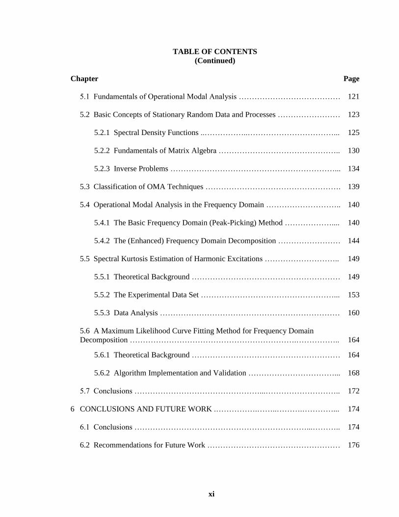
5.1 Fundamentals of Operational Modal Analysis ………………………………… 121
5.2 Basic Concepts of Stationary Random Data and Processes …………………… 123
5.2.1 Spectral Density Functions ..……………..……………………………... 125
5.2.2 Fundamentals of Matrix Algebra ……………………………………….. 130
5.2.3 Inverse Problems ………………………………………………………... 134
5.3 Classification of OMA Techniques ……………………………………………. 139
5.4 Operational Modal Analysis in the Frequency Domain ……………………….. 140
5.4.1 The Basic Frequency Domain (Peak-Picking) Method ……………….... 140
5.4.2 The (Enhanced) Frequency Domain Decomposition …………………… 144
5.5 Spectral Kurtosis Estimation of Harmonic Excitations ……………………….. 149
5.5.1 Theoretical Background ………………………………………………… 149
5.5.2 The Experimental Data Set ……………………………………………... 153
5.5.3 Data Analysis …………………………………………………………… 160
5.6 A Maximum Likelihood Curve Fitting Method for Frequency Domain
Decomposition ……………………………………………………….……………..
164
5.6.1 Theoretical Background ………………………………………………… 164
5.6.2 Algorithm Implementation and Validation ……………………………... 168
5.7 Conclusions …………………………………………...……………………….. 172
6 CONCLUSIONS AND FUTURE WORK .…………….……..……….…………... 174
6.1 Conclusions …………………………………………………………...……….. 174
6.2 Recommendations for Future Work …………………………………………… 176

xii
TABLE OF CONTENTS
(Continued)
Chapter Page
APPENDIX A CONSTRUCTION OF REINFORCED CONCRETE FRAME .…….. 178
APPENDIX B CHARACTERISTICS OF THE IRIS MOTE PLATFORMS AND
THE MEASUREMENT SENSORS EMBEDDED IN THE MTS400
CROSSBOW BOARD...…………........................................................
180
APPENDIX C 1940 EL CENTRO EARTHQUAKE RECORD ...……………..…….. 183
REFERENCES ………………………………………………………………………... 184

xiii
LIST OF TABLES
Table Page
2.1 Options Available in Lusas Bridge Plus Software ………..………..……………. 14
2.2 Design Material Properties .……….…....……………..………………………… 19
2.3 3D Flat Thin Shell Elements TTS3 Description ………...…....…………………. 21
2.4 3D Thick Beam Element BTS3 Description……………………………………... 22
2.5 Modal Frequencies of RC frame ………………………………………………… 30
2.6 Modal Frequencies of Concrete Box Section …………………………………… 48
2.7 3D Solid Continuum Elements TH4 and PN6 description ……………………… 66
2.8 Modal Frequencies of Concrete Box Section …………………………………… 81
3.1 M437A Shaker Properties ……………………………………………………….. 87
3.2 BT500M Slip Table Properties ………………………………………………….. 88
3.3 Characteristics of Microaccelerometer ADXL202 ……………………………… 90
4.1 Major Bridges Equipped with Health Monitoring Systems ……………………... 96
5.1 Comparison Between the Modal Parameters ……………………………………. 172
B.1 Technical Specifications of the IRIS mote platforms …………………………… 180
B.2 Characteristics of the Humidity and Temperature Sensor ………………………. 181
B.3 Characteristics of the Barometric Pressure and Temperature Sensor …………… 181
B.4 Characteristics of the Light Sensor ……………………………………………… 181
B.5 Characteristics of the Accelerometer Sensor ……………………………………. 182

xiv
LIST OF FIGURES
Figure Page
2.1 The investigated RC Frame …………………….........…..………………………
18
2.2 Position of steel reinforcement in RC Frame ………...…………………………..
18
2.3 RC Frame geometry defined in Lusas ………………………………………....... 20
2.4 RC Frame supports……………………………………………………………..... 20
2.5 Geometric properties of the reinforcement for beam element …………………... 22
2.6 Mesh Reinforcement Bars and Mesh Properties ……………………………….... 23
2.7 Mesh Concrete and Mesh Properties……………………….……………………. 24
2.8 Steel material properties…………………………………………………………. 25
2.9 Concrete elastic and plastic properties…………………………………………… 25
2.10 Eigenvalue Controls…………………………………………………………….... 26
2.11 The 1st mode shape ………………………………………………………………. 27
2.12 The 2nd mode shape ……………...………………………………………………. 27
2.13 The 3rd mode shape …………………...…………………………………………. 28
2.14 The 4th mode shape ………………………...……………………………………. 28
2.15 The 5th mode shape …………...…………………………………………………. 28
2.16 The 6th mode shape …………………...…………………………………………. 29
2.17 The 7th mode shape …………………...…………………………………………. 29
2.18 The 8th mode shape ……………………...………………………………………. 29
2.19 The 9th mode shape ……………………………...………………………………. 30
2.20 The 10th mode shape ………………….…………………………………………. 30

xv
LIST OF FIGURES
(Continued)
Figure Page
2.21 3-Span Concrete Box Beam bridge ……………………………………………… 31
2.22 Elevation and cross sections of the bridge ………………………………………. 32
2.23 Geometric lines and supports of the varying section bridge …………………….. 33
2.24 Concrete material properties …………………………………………………….. 33
2.25 Voided span section properties ………………………………………………….. 34
2.26 Voided intermediate section properties………………………………………...... 34
2.27 Properties of the voided section adjacent to the pier ……………………………. 35
2.28 Solid span section properties ……………………………………………………. 35
2.29 Solid pier section properties………………………………………………………
36
2.30 Column section properties ………………………………………………………. 36
2.31 Multiple varying section line properties for the Left Span ……………………… 37
2.32 Multiple varying section line properties for the Right Span …………………….. 37
2.33 Multiple varying section line properties for the Centre Span……………………. 38
2.34 Damaged section properties ……………………………………………………... 38
2.35 Location of the damage ………………………………………………………….. 39
2.36 Eigenvalue controls …………………………………………………………….... 39
2.37 HS-20 truck load ………………………………………………………………… 40
2.38 IMDPlus modal force properties ………………………………………………… 40
2.39 IMDPlus moving load analysis control ……………………………………….… 41
2.40 IMDPlus Seismic Analysis control dialog ………………………………………. 42

xvi
LIST OF FIGURES
(Continued)
Figure Page
2.41 IMDPlus Seismic output control ………………………………………………… 42
2.42 The 1st mode shape ………………………………………………………………. 43
2.43 The 2nd mode shape ……………………………………………………………… 44
2.44 The 3rd mode shape ……………………………………………………………… 44
2.45 The 4th mode shape ……………………………………………………………… 45
2.46 The 5th mode shape ……………………………………………………………… 45
2.47 The 6th mode shape ……………………………………………………………… 46
2.48 The 7th mode shape ……………………………………………………………… 46
2.49 The 8th mode shape ……………………………………………………………… 47
2.50 The 9th mode shape ……………………………………………………………… 47
2.51 The 10th mode shape …………..………………………………………………… 48
2.52 Displacement time history of the mid-span for truck speed of 15 m/s ………….. 49
2.53 Acceleration of the mid-span for truck speed of 15 m/s ………………………… 49
2.54 Peak vertical displacement response of the mid-span …………………………… 50
2.55 Peak vertical acceleration response of the mid-span ……………………………. 50
2.56 Displacement time history of the mid-span for truck speed of 15 m/s ………….. 51
2.57 Acceleration of the mid-span for truck speed of 15 m/s ………………………… 51
2.58 Peak vertical displacement response of the mid-span …………………………… 52
2.59 Peak vertical acceleration response of the mid-span ……………………………. 52
2.60 Displacement time history of the mid-span under El Centro earthquake ……….. 53

xvii
LIST OF FIGURES
(Continued)
Figure Page
2.61 Peak displacements output ………………………………………………….…… 54
2.62 Aerial Photo of the bridge ……………………………………………………….. 55
2.63 Side view of the bridge…………………………………………………………... 56
2.64 Geometry of the bridge…………………………………………………………... 57
2.65 Precast Segmental Box Girder Bridge modeled in Lusas Bridge Plus software… 59
2.66 Properties of A_A section adjacent to the abutments …………………………… 60
2.67 Voided B_B section properties ………………………………………………….. 60
2.68 Voided C_C section properties ………………………………………………….. 61
2.69 Voided D_D section properties …………………………………………………. 61
2.70 Solid section properties at abutments …………………………………………… 62
2.71 Solid section properties at piers …………………………………………………. 62
2.72 Varying section of the bridge ……………………………………………………. 63
2.73 Multiple varying section line properties for 5th span …………………………… 64
2.74 Multiple varying section line properties for 5th span …………………………… 64
2.75 Bridge piers geometry …………………………………………………………… 65
2.76 Bridge piers Mesh ……………………………………………………………….. 66
2.77 Typical uniaxial compressive and tensile stress-strain curve for concrete ……… 67
2.78 Concrete material properties …………………………………………………….. 68
2.79 AASHTO LRFD design lane load description ………………………………….. 69
2.80 AASHTO LRFD design lane load applied to the bridge model ………………… 69

xviii
LIST OF FIGURES
(Continued)
Figure Page
2.81 Moving load generator ………………………………………………...………… 70
2.82 AASHTO LRFD HS-20 truck load …………………………...………………… 70
2.83 Moving HS-20 truck on the bridge FE model ………………………………..…. 71
2.84 Eigenvalue controls ……………………………………………………………… 71
2.85 Deformed mesh under gravity Load …………………………………………….. 72
2.86 Deformed mesh under Lane Load ……………………………………………….. 72
2.87 Deformed mesh under HS-20 truck load ………………………………………... 73
2.88 Deformed Mesh for positive displacement envelope under HS-20 truck load…... 73
2.89 Deformed Mesh for negative displacement envelope under HS-20 truck load….. 73
2.90 Moment Diagram under gravity load ……………..…………………………….. 74
2.91 Moment Diagram under lane load ………………………………………………. 74
2.92 Moment Diagram under HS-20 truck load ……………………………………… 74
2.93 Positive Moment Diagram envelope under HS-20 truck moving load ………….. 75
2.94 Negative Moment Diagram envelope under HS-20 truck moving load ………… 75
2.95 Stress Contour S(x) of bridge deck under gravity load …………………………. 75
2.96 Stress Contour S(x) of bridge deck under lane load …………………………….. 76
2.97 Stress Contour S(x) of bridge deck under moving HS-20 truck load …………… 76
2.98 Stress Contour S(z) of bridge piers under gravity load ………………………….. 76
2.99 The 1st mode shape ………………………………………………………………. 77
2.100 The 2nd mode shape ……………………………………………………………… 78

xix
LIST OF FIGURES
(Continued)
Figure Page
2.101 The 3rd mode shape ……………………………………………………………… 78
2.102 The 4th mode shape ……………………………………………………………… 79
2.103 The 5th mode shape ……………………………………………………………… 79
2.104 The 6th mode shape ……………………………………………………………… 79
2.105 The 7th mode shape ……………………………………………………………… 80
2.106 The 8th mode shape ……………………………………………………………… 80
2.107 The 9th mode shape ……………………………………………………………… 80
2.108 The 10th mode shape …………..………………………………………………… 81
3.1 The investigated RC frame ……………………………………………………… 84
3.2 Position of steel reinforcement in RC frame …………………………………….. 84
3.3 Sine excitation of shaking table ………....….………..………………………….. 85
3.4 Wireless sensors arrangement mounted on RC frame ...………………………… 86
3.5 RC frame mounted on the shaking table ..…..………………………….………... 86
3.6 IRIS mote board top and bottom view …………………………………………... 88
3.7 MIB520 USB interface board …………………………………………………… 89
3.8 Front and back view of the MTS400 sensors’ board ……………………………. 90
3.9 Acceleration data recorded under 5 Hz excitation ………………………………. 91
3.10 Acceleration data recorded under 13 Hz excitation ……………………………... 92
3.11 Acceleration data recorded under 20 Hz excitation ……………………………... 92
4.1 Advantages and Disadvantages of strain gauges ……...………………………… 103

xx
LIST OF FIGURES
(Continued)
Figure Page
4.2 Fiber optic versus vibrating wire Sensors ……………………………………….. 107
4.3 Wireless network topology ……………………………………………………… 111
4.4 Schematic Layout of the Accelerometers ………………………………...……... 116
4.5 Distribution of strain gauges in the bridge ……………………….……………… 117
4.6 Locations of Temperature sensors for long-term monitoring …………………… 118
5.1 Discrete Fourier Transform of a rectangular window …………………………… 129
5.2 SK expectations as function of duty-cycle ………………………………………. 152
5.3 Data set without background noise ……………………………………………… 154
5.4 Data in the presence of added noise ……………………………………………... 154
5.5 Decimated time series and PSD for 1024 samples without damage …………….. 155
5.6 Decimated time series and PSD for 1024 samples with damage ………………... 155
5.7 Damaged detected using both SK analysis and classical spectrum analysis ……. 156
5.8 SK-S1 diagram without and with damage based on the bridge dynamic response 157
5.9 SK-S1 diagram based on the bridge dynamic response due to the moving truck .. 158
5.10 SK-S1 diagram based on the bridge dynamic response due to earthquake ……... 159
5.11 SK estimators corresponding to the two input force data channels ……………... 160
5.12 SK estimators corresponding to the first two response data channels …………... 161
5.13 Automatic harmonic line identification …………………………………………. 162
5.14 Illustration of the automated ML FDD algorithm steps …………………………. 169
A.1 Reinforcement assembly ………..……………………………………………….. 178

xxi
LIST OF FIGURES
(Continued)
Figure Page
A.2 The wood works and reinforcement for the RC frame ………………………….. 178
A.3 Preparation of the concrete ……………………………………………………… 179
A.4 Pouring the concrete …………………………………………………………….. 179
A.5 Curing of the frame ……………………………………………………………… 179
C.1 Ten second sample of the ground motion accelerograms ……………………….. 183

1
CHAPTER 1
INTRODUCTION
1.1 Structural Health Monitoring
All structures, including critical civil infrastructure facilities like bridges and highways,
deteriorate with time. This deterioration is due to various reasons including fatigue failure
caused by repetitive traffic loads, effects of environmental elements, and extreme events
such as earthquake, tornados and sever wind. In recent years, the situation of aging
infrastructure has become a global concern. This is especially true in the case of highway
bridges in the United States, because a large number of structures in the current bridge
inventory were built decades ago and are now considered structurally deficient [1].
According to December 2011 data reported by U.S. Department of Transportation-Federal
highway administration (FHWA), among total of 605,086 bridges all over the United States
more than 23% of the bridges are classified as deficient. Among which 11.15% of them
are structurally deficient and 12.62% functionally obsolete. In another report prepared by
the American Society of Civil Engineers (ASCE) in 2013[2], there was approximately
$20.5 billion of total investment estimated for full restoration of bridges annually. This
number is expected to grow as more than 30 percent of the existing bridges have exceeded
their 50-year theoretical design life and are in various levels of repair, rehabilitation,
replacement or even decommissioned [3].
In order to maintain the safety of these “lifeline” structures, each state has been
mandated by the National Bridge Inspection (NBI) program to periodically inventory and
inspect all highway bridges on public roads. Implemented in 1971, The National Bridge
Inspection Standards prescribe minimum requirements for the inspection of highway

2
bridges in the United States [4]. A substantial amount of research has been conducted in
this area in order to improve the speed and reliability of such inspections. According to
another survey performed by the Federal Highway Administration [5], visual inspection is
still the primary tool used to perform these inspections. The implementation of these
inspections consists of scheduled field trips to bridge sites at routine intervals, usually once
every two years. If a significant increase in distress between inspections is noted, the period
between inspections is decreased and the level of inspection is increased till such time that
the distress has been corrected by repair or replacement. Research has shown that such
inspections have limited accuracy and efficiency [6]. This method of time-based inspection
is inefficient in terms of resources, because all bridges are inspected with the same
frequency, regardless of the condition of the bridge. Moreover, there is a potential danger
that serious damage could happen to the bridge in between two inspections which pose a
great hazard to public safety. Visual inspections are highly variable, lack resolution, and
fail to detect damage unless it is visible [7]. Furthermore, rapid assessment of structural
conditions after major events such as earthquakes is not possible using such approach. As
a result, structurally deficient and functionally obsolete bridges may be left undiscovered,
potentially putting the public at risk. Therefore, more automated and reliable methods of
inspection are necessary.
Over the past decade, the implementation of Structural Health Monitoring (SHM)
systems has enhanced as a potential solution to the above challenges. SMH is a mature
research field that investigates the current condition of structures by measurement, modal
analysis, and condition assessment. It refers to implementation of damage identification
strategies to the civil engineering infrastructures [8]. Damage means the degradation of the

3
performance of the structure which is mainly due to change in material and geometric
properties, boundary conditions and system connectivity. SHM strives toward the ideal of
not only be able to monitor a structure in such a way that any damage or any growth of
fault would be immediately detectable, but also assessing the severity so that decisions can
be easily made about what actions need to be taken.
These global objectives for SHM are generally structured into the following levels:
Damage detection: the method that gives a qualitative indication that damage might
be present in the structure.
Damage Location: The method that gives information about the probable position
of the damage.
Damage Classification: The method that gives information about the type of
damage.
Damage Assessment: The method that gives an estimate of the extent of the
damage.
Damage Prediction: The method that offers information about the safety of the
structure, e.g., life span estimate.
Structures are designed to perform well under certain loading and environmental
conditions with certain lifespan. However, the actual situation might not always be the
same. Performance of structures degrades with time and moreover, there might be some
uncertainties involved, such as seismic events, tsunamis or explosions. Structural Health
Monitoring helps us to keep track of the performance level of the structures by improving
safety and maintaining its functionality. After the occurrence of any catastrophic events
such as an earthquake or explosions there is no quantifiable method to check whether the
buildings are safe to reoccupy or the bridges are safe to use [8]. The continuous automated

4
SHM can be a solution for the above mentioned problem. With automated monitoring
systems in place on critical life-line structures, the condition of these structures can be
monitored and evaluated shortly after an extreme event has occurred. This rapid evaluation
would not be possible using traditional inspection techniques. Necessary decisions to best
utilize the remaining intact life-lines can be made based on these evaluations. This could
potentially give the authority faster access to the affected areas and thus improving public
safety. As the principles of SHM and its applications is not only in the inspection of existing
infrastructure but also lifetime monitoring of future construction projects [9]. There has
been an increase interest in SHM by infrastructure stakeholders due to its high potential for
the economic benefits and life safety of the users. Numerous SHM methods have been
proposed in recent years; detailed reviews are provided by [10, 11].
1.2 Vibration Based Damage Detection Strategy
The various disciplines utilize different approaches in SHM. The first successful attempts
have been taken by the mechanical engineers using analysis of vibrations for the prediction
of damage of machinery during the late 1970s. Few years later, the automobile and
aerospace industry discovered the advantages of diagnosis systems. In these disciplines,
SHM profits from the very well-defined material properties and geometries. Also, the
objectives are very similar from case to case and stable routines was developed. The
practice has focused on the detection of crack and fatigue indicators in aircraft bodies and
machinery.
Bridges are structures that have very little in common with each other. Almost any
new bridge is a prototype. The combination of facts, use, properties, boundary conditions
and geometry create a huge number of unknowns. As a result, a uniform monitoring

5
process is not feasible. There is an extensive difference between civil engineering and all
the other disciplines. In mechanical engineering, automotive or aeronautics monitoring
systems are designed to work permanently over the lifetime of a structure or component.
In civil engineering, this is not feasible financially. Most of civil structures already exist
with a widely unknown history. Therefore, considerable educational effort is necessary to
support the requirements of realistic damage detection and assessment.
During the last three decades, a great deal of research has been conducted in the
field of Vibration-Based Structural Health Monitoring. A broad range of techniques,
algorithms and methods were developed to solve damage identification problems in
structures, from basic structural components such as beams and plates to complex structural
systems like bridges and high-rise buildings.
Most non-destructive damage identification methods can be categorized as either
local or global damage identification techniques [10]. Local damage identification
techniques, such as ultrasonic methods and X-ray methods, require a priori information of
damage locations. Locating procedure using these methods is often time consuming and
expensive and cannot be guaranteed for most cases in civil engineering. Furthermore,
Nondestructive Evaluation requires detailed scanning of each structure member; which is
not feasible for large scale structures. Hence, the dynamic-based damage identification
method, as a global damage identification technique was developed to overcome these
difficulties. The dynamic-based damage identification is based on the idea that damage
causes changes in structural parameters such as mass, damping, stiffness and flexibility.
This will lead to changes in the dynamic structure’s properties and vibration modal
parameters such as natural frequency, modal damping and mode shapes. Therefore,

6
damage can be identified by analyzing the changes in dynamic features of the structure.
This makes the vibration-based method suitable for SHM system for large civil
infrastructures.
1.3 Operational Modal Analysis
From the discussion in the previouse Section, it becomes clear that the measurement of
structural dynamic properties such as modal parameters is an important step in vibration-
based structural health monitoring. The use of experimental tests to gain knowledge about
the dynamic response of civil structures is a well-established practice. The experimental
identification of the modal parameters can be dated back to the middle of the Twentieth
Century [12]. As mentioned before, that the dynamic behavior of the structure can be
demonstrate as a combination of modes that each one characterized by a set of parameters
such as natural frequency, damping ratio and mode shapes whose values depend on the
structure’s geometry, material properties and boundary conditions. Traditional
Experimental Modal Analysis (EMA) identifies those parameters from measurements of
the applied force and the vibration response. EMA makes use of measured input excitation
as well as output response and has made substantial progress in the past three decades.
Numerous modal identification algorithms have been developed and applied in various
fields such as vibration control, structural dynamic modification, and analytical model
validation, as well as vibration-based structural health monitoring in mechanical, aerospace
and civil applications. However, Traditional Experimental Modal Analysis suffers some
Limitations such as:
Need of an artificial excitation in order to measure Frequency Response Functions
(FRF) or Impulse Response Functions (IRF);

7
Operational conditions often different from those ones applied in the lab
environment tests;
Simulated boundary conditions, since tests are carried out on components instead
of complete systems.
The identification of the modal parameters by EMA techniques becomes more
challenging in the case of civil engineering structures because of their large size and low
frequency range. It is typically very difficult to excite the structure using controlled input
and requires expensive and heavy devices which increases the risk of damaging the
structures. As a consequence, since early 1990’s Operational Modal Analysis (OMA) has
drawn significant attention in the field of civil engineering with applications on several
structures (buildings, bridges, off-shore platforms, etc.).
OMA utilizes only response measurements of the structure under operational or
ambient conditions to identify modal parameters. The idea behind OMA is to take
advantage of the natural and freely available excitation due to ambient forces and
operational loads (wind, traffic, micro-tremors, etc.) which makes it particularly attractive
for vibration-based bridge health monitoring applications because the bridge does not need
to be closed to traffic to perform the modal parameter identification. In other words, the
identified modal parameters are representative of the actual behavior of the structure in its
operational conditions, since they refer to levels of vibration actually present in the
structure and not to artificially generated vibrations. Due to these reasons, it has become
the method of choice for identification of structural modal parameters in long-term
Vibration-based Structural Health Monitoring applications. OMA is also known under

8
different names, such as ambient vibration modal identification or output-only modal
analysis.
Over the years, Operational Modal Analysis advanced as an independent discipline,
but most of the OMA methods have been derived from EMA procedures, so they share a
common theoretical background. The main difference is the formulation of input which is
known in EMA while it is random and not measured in OMA. EMA procedures are
developed in a deterministic framework while OMA methods are based on random
response and stochastic approach. In Operational Modal Analysis input is assumed to be a
Gaussian white noise and characterized by a flat spectrum in frequency domain. In this
way, all nodes are assumed to be equally excited in the frequency range of interest and
extracted by appropriate procedure. Both EMA and OMA techniques can be categorized
in frequency domain or time domain methods.
Despite of the differences in terms of excitation, modal analysis is always based on
the following steps:
planning and execution of tests: this step concerns the definition of the experimental
setup such as: proper location of sensors and the data acquisition parameters.
data processing and identification of modal parameters (filtering, decimation,
windowing; extraction of modal parameters); this step concerns the validation and
pre-treatment of the acquired data, and the estimation of the modal parameters.
validation of the modal parameter estimates.
The final objective of the test is not the estimation of modal parameters. In fact,
these parameters can be used as input or reference for a number of applications. Model
updating is probably the most common [13]. Since the modal parameters estimates
provided by Finite Element models are not often reliable, the numerical model is not the

9
representative of the actual dynamic behavior of the structure. As a result, the experimental
modal properties are used to enhance a FE model of the structure in order to make it more
adherent to the structure’s actual behavior.
Additionally, the identified modal parameters are sometimes used for
troubleshooting by using the identified vibrational properties to find out the cause of
problems often encountered in real life such as excessive noise or vibrations. Also the
estimated modal parameters can be used for sensitivity analyses to evaluate the effect of
changes on the dynamics without actually modifying the structure [12]. Furthermore, some
applications concern force identification. In this case, the known modal parameters are
used to solve an inverse problem for the identification of the unknown forces that produced
a given measured response [14].
Another relevant application of the identified modal parameters is damage
detection and structural health monitoring. Indications of presence of damage on the
structure can be obtained after comparing current modal parameters of the structure with
the modal parameters at a reference state. With the developments of methods in the last
few years not only the damage can be detected, but also it can be located and quantified.
Extensive reviews about these techniques are available in these literatures [10, 11, 15].
The main drawback of damage detection techniques based on the analysis of the
changes in the estimated modal properties is that significant changes in modal frequencies
cannot imply presence of damage due to the influence of boundary conditions and
operational and environmental factors on the estimates. However, in recent years a number
of techniques have been developed by monitoring environmental conditions together with
the structural response, which enables them to remove the influence of environmental

10
factors on modal parameter estimates [16, 17]. As a result, raising interest towards
vibration-based damage detection has been renewed. Another relevant limitation to the
extensive application of these damage detection techniques was the lack of fully automated
procedures for the estimation of the modal parameters of the monitored structure. This
issue has determined large research efforts in the last few years to develop reliable and
robust automated OMA techniques [13].
1.4 Research Objectives
The previous section presents the state-of-the-art in the technical background of the
Structural Health Monitoring. The research proposes a development of a long term
monitoring system for damage detection and real-time monitoring. In this research three
main aspects are considered. The first one is the development of an improved method for
damage localization, identification, and detection in SHM. The second one is the optimal
design of Wireless Sensor Networks for SHM monitoring. Finally, the third one is the
improvement of the reliability of the monitoring and predict the capacity and remaining
life of the structure.
This research provides deeper insight into the utilization of WSNs for SHM
including the sensing techniques, optimization of WSNs design particularly for SHM
monitoring and damage detection techniques. The proposed system will not only aim to
detect damage after it happens but it will also aim to predict damage before it takes place.
The data obtained from the research will result in a reduction in the lifecycle costs and risks
related to bridge structures.

11
The proposed technique will eventually be applied to the new stadium that State of
Qatar will build in preparation for the 2022 World Cup. This monitoring system will help
permanently record the vibration levels reached in all substructures during each event to
evaluate the actual health state of the stadiums. This offers the opportunity to detect
potentially dangerous situations before they become critical.
1.5 Thesis Overview
This thesis consists of six chapters. The layout of the thesis document is presented as
follows:
Chapter 1, the current chapter, presents the introduction of the work referring the
motivation, the general background of Structural Health Monitoring topics as well as the
objectives of this research.
Chapter 2 presents Finite Element Analysis (FEA) of a scaled down Reinforced
Concrete Frame, 3-Span Bridge and an In-service 6-Span Precast Segmental Box Girder
Bridge. The mode shapes of all structures are obtained from eigenvalue frequency analysis.
For the 3-Span Bridge, Moving Load analysis has been carried out and Seismic Response
of the bridge under El Centro earthquake ground motion is presented. The later sections of
the chapter provides Static and Dynamic Finite Element analysis of 6-Span Concrete Box
Girder Bridge. Analysis results for each model thoroughly demonstrated in each section.
Chapter 3 is dedicated to a preliminary study in designing and setting up a test-bed
for the research on Structural Health Monitoring utilizing Wireless Sensor Networks. The
design and setup of the physical model are presented in detail. Three different excitation
cases has been investigated to evaluate the performance of the developed wireless sensing
system under actual experimental conditions.

12
Chapter 4 outlines the design criteria of SHM for a large-scale bridge. The available
technologies on measurement sensors and data acquisition equipment for performing long
term monitoring is then introduced. Special emphasis is given to the wireless based systems
presenting their state of the art and their current and past applications for monitoring civil
engineering structures. In this chapter, a long-term Structural Health Monitoring System
using Wireless Sensor Networks (WSNs) for an in-service highway bridge is also devised.
Chapter 5 presents the theoretical basis of the Operational Modal Analysis. Here, it
is shown that higher order statistical estimators such as Spectral Kurtosis (SK) and Sample
to Model Ratio (SMR) can be successfully employed to more reliably discriminate the
response of the system against the ambient noise fluctuations and to better identify and
separate contributions from closely spaced individual modes. Moreover, it is shown that a
SMR-based Maximum Likelihood curve fitting algorithm improves the accuracy of the
spectral shape and location of the individual modes.
Chapter 6 presents the conclusions of the thesis as well as the proposal of future
developments.

13
CHAPTER 2
FINITE ELEMENT ANALYSIS
2.1 Introduction
The Lusas Bridge Plus finite element program, operating on Windows 8, was used in this
study to simulate the behavior of an experimental frame, 3-Span Bridge and an in-service
6-Span Precast Segmental Box Girder Bridge. In general, the conclusions and methods
would be very similar using other nonlinear Finite Element Analysis programs. Each
program, however, has its own nomenclature and specialized elements and analysis
procedures that need to be used properly. Which requires the analyst to be thoroughly
familiar with the finite element tools being used, and progress from simpler to more
complex problems in order to gain confidence in the use of new techniques.
This chapter discusses model development for aforementioned structures. Element
types used in the models are covered along with the constitutive assumptions and
parameters for the various materials in each Section. Besides, Geometry of the models,
loading and boundary conditions are presented. The reader can refer to a wide variety of
finite element analysis textbooks for a more formal and complete introduction to basic
concepts if needed.
2.2 Lusas Bridge Software
LUSAS Bridge is a world-leading finite element analysis software for the analysis, design
and assessment of all types of bridge structures. LUSAS Bridge provides all the facilities
needed to carry out from a straightforward linear static analysis of a single span road bridge,
to a dynamic analysis of a slender ‘architectural’ steel movable footbridge, or a detailed

14
geometrically nonlinear staged erection analysis of a major cable stayed structure involving
concrete creep and shrinkage. LUSAS Bridge is available in a choice of software levels;
Bridge LT, Bridge, and Bridge Plus to suit different analysis needs. Bridge Plus version
has been selected to use in this research which has outstanding range of analysis facilities
for linear static, fundamental frequency, seismic, dynamic, soil-structure interaction, large
deflection, staged construction, creep, pre-stress, post tensioning and fatigue analysis.
Moreover, Plus versions allow for more advanced analyses to be undertaken and include
an extended high-performance element library. A list of software options available in Lusas
Bridge plus version is given in Table 2.1. In order to facilitate the discussion in the later
parts of this chapter, it is necessary to provide a brief review of some of the features of
Lusas Bridge Plus that have been utilized in this research.
Table 2.1 Options Available in Lusas Bridge Plus Software
LUSAS Bridge Plus Software Option
Fast Solvers
Vehicle Load Optimization
Steel and Composite Deck Designer
IMDplus Analysis
Nonlinear Analysis
Dynamic Analysis
Thermal / Field Analysis
Heat of Hydration Analysis
Rail Track Analysis
Two types of fast solvers implemented in this software which are Multifrontal
Direct Solver and Multifrontal Block Lanczos EigenSolver. The Fast Multifrontal Direct
Solver is an implementation of the multifrontal method of Gaussian Elimination, and uses

15
the modern sparse matrix technology of assembling a global stiffness matrix where only
the non-zero entries are stored. The solver can be used for almost all types of analysis, and
has extensive pivoting options to ensure numerical stability, especially for symmetric
problems. As a result, it is particularly fast at solving large 3D solid models and the disk
space requirements are typically 75% less than that of the standard frontal direct solvers.
Additionally, a data check facility with the standard Frontal Direct solver which enables
rerunning linear analyses with different load cases without having to eliminate the stiffness
matrix. The Fast Multifrontal Block Lanczos Eigensolver is based on the Shift and Inverse
Block Lanczos algorithm and solves natural frequency, vibration and buckling problems
with real, symmetric matrices. It is fast, robust, and ensures that convergence is almost
always achieved. For instance, the lowest, highest or a range of eigenvalues can be
specified to be returned, along with the normalized eigenvectors and error norms which are
currently given with the standard Frontal Eigensolvers. In other words, you can specify
combinations of eigenvalues to be returned in the same analysis, as for example, the highest
three eigenvalues can be specified, followed by the lowest ten, and all those in the range 0
to 50. The complex eigensolver is non-symmetric eigensolver based on an implicitly
restarted Arnoldi method. It provides solutions to damped natural frequency problems for
both solid and fluid mechanics. It can solve large scale problems with real, non-symmetric
input matrices (in particular, those involving non-proportional damping), and gives
solutions that consist of complex numbers where appropriate.
Vehicle Load Optimization software complements and extends the in-built static
and moving vehicle loading capabilities of LUSAS Bridge and helps to significantly
simplify the evaluation of worst load position for various load configurations. It is used to

16
identify critical vehicle loading patterns on bridges and apply these loading patterns to
LUSAS analysis models. It reduces the amount of time spent generating models and leads
to more efficient and economic design, assessment or load rating of bridge structures.
Vehicle Load Optimization works with numerous country design codes such as:
United States of America: AASHTO LFD, LRFD
United Kingdom: EN1991-2, BD21/97, BD21/01, BD37/88, BD37/01
(Road+Rail), BS5400 Rail Railtrack document RT/CE/025
Europe: EN1991-2
Canada CAN/CSA-S6-06
The IMDPlus option extends the Interactive Modal Dynamics (IMD) techniques
available in LUSAS software. While, IMD models a single loading event in a single
direction, IMDPlus allows multiple loading events with more advanced loading conditions
to be solved. IMDPlus is applicable to both 2D and 3D structures and has three primary
uses:
Moving load analysis of structures, such as bridges subjected to moving
vehicle or train loads, where the magnitude and configuration of the loading
remains constant throughout the analysis.
Moving mass and moving sprung mass analysis of structures, such as bridges
subjected to moving vehicle or train loads, where mass-spring-damper systems
are used to represent the vehicle. The configuration of the systems remains
constant throughout the analysis but, as they move across the structure, the
dynamic response of the unsprung and sprung masses affects the applied
loading due to inertia effects.
Seismic Response analysis of structures subjected to acceleration time
histories of support motion.

17
An IMDPlus analysis uses conventional eigenvalue analyses to obtain the
undamped modes of vibration for a structure over the frequency range of interest. The
modal response in the form of frequencies, participation factors and eigenvectors, together
with the seismic accelerations or moving load/moving mass vehicle loads, enable IMDPlus
to compute the dynamic response for each mode of vibration. The assumption of linear
structural behavior allows the IMDPlus facility to utilize linear superposition methods to
calculate the total response of the structure from each of the contributing frequencies.
The LUSAS Dynamics Option contains the facilities required to solve a wider range
of dynamic problems in both the time and frequency domains. By combining the LUSAS
Dynamic and LUSAS Nonlinear options, both high and low velocity nonlinear impact
problems can be solved using either implicit or explicit solution techniques. By combining
the LUSAS Dynamic and LUSAS Thermal options, time-domain analyses such as
Transient Field can be carried out.
LUSAS Bridge is used by structural engineers worldwide for all types of bridge
analysis, design and load rating. There are numerous Case studies in the literature which
provide a number of uses of Lusas Bridge software[18].

18
2.3 Analysis of a Reinforced Concrete Frame
The Reinforced Concrete Frame modeled in this section had span of 32.5 cm (12.8 in) and
height of 24.5 cm (9.6 in) as shown in Figure 2.1. The frame properties are: The modulus
of elasticity 𝐸𝑐 = 31.58MPa (4500 psi), mass per unit volume M = 2400 kg/m3 (150 lb/scf),
cross-section dimensions 5 × 5 cm for an area A = 25 cm2, #2 (6 mm diameter) for Steel
rebar, for stirrups diameter of 3 mm and 1 cm concrete cover. Figure 2.2 shows the frame
dimensions and the location of the rebar. Table 2.2 shows the material properties used for
analysis.
Figure 2.1 The investigated RC Frame.
Figure 2.2 Position of steel reinforcement in RC Frame (Dimensions are in cm).

19
Table 2.2 Design Material Properties.
Material Limiting Stress Limiting Strain Limit State Elastic Modulus
Concret
(Compre
ssion)
4500 psi
(31.58 MPa )
0.003 Crushing 6000 𝑘𝑠𝑖1
(42 GPa)
Steel
Reinforc
ement
60 ksi
(414 MPa)
0.002 Yielding 29,000(200 GPa)
¹ Design elastic modulus from 𝐸𝑐 = 57,000(𝑓𝑐’)1/2.
2.3.1 Modeling Description
A Natural Frequency Analysis is to be carried out on a model of a Reinforced Concrete
Frame. As mentioned before, the reinforcement is provided in the beam and columns has
a total cross-sectional area of 1.13 𝑐𝑚2 (0.444 in2). The superposition of nodal degrees of
freedom assumes that the concrete and reinforcement are perfectly bonded. It is assumed
that the effects of any shear reinforcement can be ignored.
Due to the symmetrical nature of the problem, only the left-hand span of the frame
is modelled (see Figure 2.3). The column support is fixed at the left-hand of the frame with
a symmetry support at the right-hand axis of symmetry as shown in Figure 2.4.

20
Figure 2.3 RC Frame geometry defined in Lusas.
Figure 2.4 RC Frame supports.
No static structural loading is required for this analysis because only the dynamic
loading is considered during the results processing based on the results from the natural
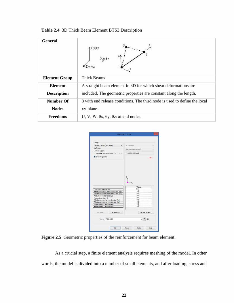
frequency analysis. The concrete section is represented by Thick Shell (TTS3) elements,
and the reinforcement bars are represented by nonlinear Beam (BTS3) elements and then
as presented in Figure 2.5 the actual geometric properties of the reinforcement has been
applied to the element, See Tables 2.3 and 2.4 for more element details. A nonlinear

21
concrete cracking material model is applied to the thick shell elements and a von Mises
plastic material is applied to the reinforcement bars. Units of N, mm, t, s, C are used
throughout the finite element modeling of this frame.
Table 2.3 3D Flat Thin Shell Elements TTS3 Description
General
Element Group Thick Shells
Element
Description
A family of shell elements for the analysis of arbitrarily thick and thin
curved shell geometries, including multiple branched junctions. The
quadratic elements can accommodate generally curved geometry while
all elements account for varying thickness. Anisotropic and composite
material properties can be defined. These degenerate continuum elements
are also capable of modelling warped configurations. The element
formulation takes account of membrane, shear and flexural deformations.
This elements use an assumed strain field to define transverse shear
which ensures that the element does not lock when it is thin.
Number Of
Nodes
3, numbered anticlockwise.
Freedoms Default: 5 degrees of freedom are associated with each node U, V, W,
θα, θβ. To avoid singularities, the rotations θα and θβ relate to axes
defined by the orientation of the normal at a node. Degrees of freedom
relating to global axes: U, V, W, θx, θy, θz may be enforced using the
Nodal Freedom data input, or for all shell nodes by using option 278.
Notes For TTS3 elements all moments and shears are constant for the element.
22
Table 2.4 3D Thick Beam Element BTS3 Description
General
Element Group Thick Beams
Element
Description
A straight beam element in 3D for which shear deformations are
included. The geometric properties are constant along the length.
Number Of
Nodes
3 with end release conditions. The third node is used to define the local
xy-plane.
Freedoms U, V, W, θx, θy, θz: at end nodes.
Figure 2.5 Geometric properties of the reinforcement for beam element.
As a crucial step, a finite element analysis requires meshing of the model. In other
words, the model is divided into a number of small elements, and after loading, stress and
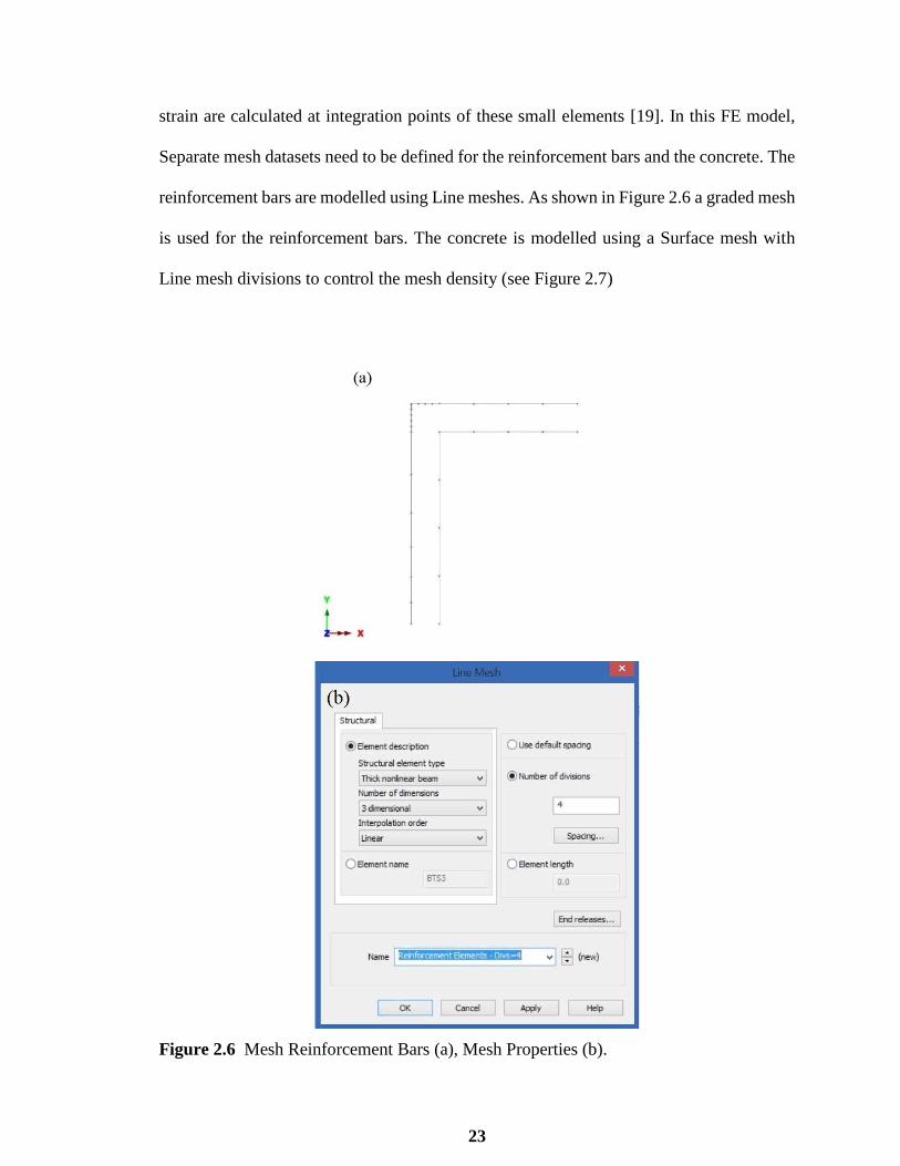
23
strain are calculated at integration points of these small elements [19]. In this FE model,
Separate mesh datasets need to be defined for the reinforcement bars and the concrete. The
reinforcement bars are modelled using Line meshes. As shown in Figure 2.6 a graded mesh
is used for the reinforcement bars. The concrete is modelled using a Surface mesh with
Line mesh divisions to control the mesh density (see Figure 2.7)
Figure 2.6 Mesh Reinforcement Bars (a), Mesh Properties (b).

24
(a)
(b)
Figure 2.7 Mesh Concrete (a), Mesh Properties (b).
Nonlinear steel properties has been defined for the reinforcing Bar elements and
nonlinear concrete material properties for the Surface elements representing the concrete
as illustrated in Figures 2.8 and 2.9 respectively.

25
Figure 2.8 Steel material properties.
(a)
(b)
Figure 2.9 Concrete elastic (a) and plastic (b) properties.

26
The modelling is completed by defining the controls necessary to extract the natural
frequencies. Eigenvalue controls are defined as properties of the loadcase utilizing the
IMDPlus option in Lusas (see Figure 2.10). The working assumptions for the IMDPlus
modal dynamics facility are as follows:
The system is linear in terms of geometry, material properties and boundary
conditions. Therefore, geometrically nonlinear eigenvalue results are not applicable.
Nor are nonlinear joint and slideline analyses suitable for this type of post-
processing treatment.
There is no cross-coupling of modes caused by the damping matrix. This is
reasonable for all but the most highly damped structures or applications.
Figure 2.10 Eigenvalue Controls.
2.3.2 Natural Frequency Analysis Results
The mode shapes obtained from eigenvalue frequency analysis are plotted in Figures 2.11-
2.20. The first two vibrational modes are transverse modes and the third mode is the first
vertical mode. Moreover, the first mode of the frame was found to have frequency of
298.78 Hz (Figure 2.11), the second mode was found to be at 756.96 Hz (Figure 2.12).
Eigenvalue results of the first 10 mode shapes for the whole structure are displayed in Table
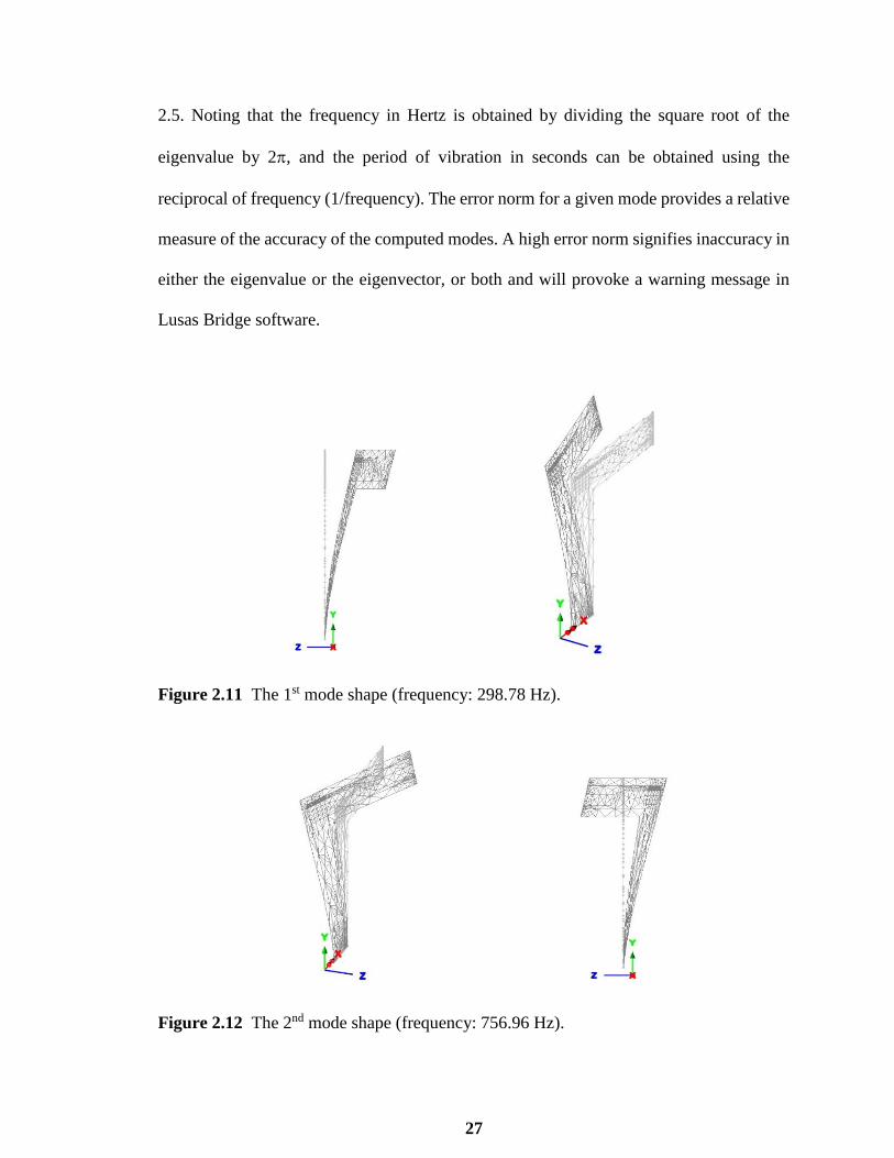
27
2.5. Noting that the frequency in Hertz is obtained by dividing the square root of the
eigenvalue by 2, and the period of vibration in seconds can be obtained using the
reciprocal of frequency (1/frequency). The error norm for a given mode provides a relative
measure of the accuracy of the computed modes. A high error norm signifies inaccuracy in
either the eigenvalue or the eigenvector, or both and will provoke a warning message in
Lusas Bridge software.
Figure 2.11 The 1st mode shape (frequency: 298.78 Hz).
Figure 2.12 The 2nd mode shape (frequency: 756.96 Hz).
28
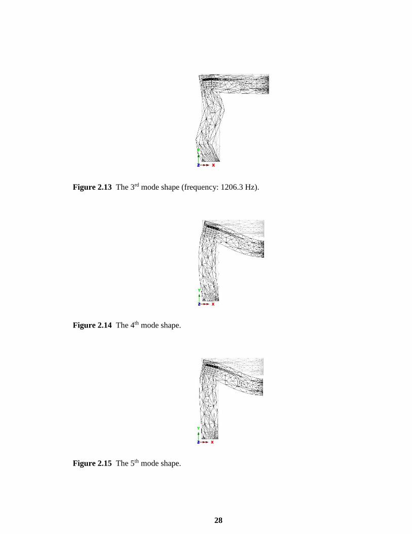
Figure 2.13 The 3rd mode shape (frequency: 1206.3 Hz).
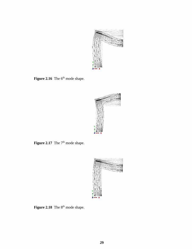
Figure 2.14 The 4th mode shape.
Figure 2.15 The 5th mode shape.
29
Figure 2.16 The 6th mode shape.
Figure 2.17 The 7th mode shape.
Figure 2.18 The 8th mode shape.

30
Figure 2.19 The 9th mode shape.
Figure 2.20 The 10th mode shape.
Table 2.5 Modal Frequencies of RC frame
Mode Eigenvalue Frequency (Hz) Error Norm
1 0.352416E+07 298.778 0.998320E-10
2 0.226209E+08 756.964 0.209138E-10
3 0.574492E+08 1206.32 0.840491E-11
4 0.103503E+09 1619.18 0.134112E-10
5 0.113124E+09 1692.77 0.103542E-10
6 0.136238E+09 1857.67 0.140018E-10
7 0.138146E+09 1870.63 0.915716E-11
8 0.138281E+09 1871.55 0.157550E-09
9 0.251601E+09 2524.50 0.476150E-06
10 0.254828E+09 2540.64 0.139250E-06

31
2.4 Analysis of 3-Span Concrete Box Beam Bridge of Varying Section
A 3-Span Concrete Box Beam Bridge of varying cross-section is modelled using the box
section property calculator and the multiple varying sections facilities in LUSAS (Figure
2.21).
Figure 2.21 3-Span Concrete Box Beam bridge.
Two models are created suitable for prototype / assessment work; a preliminary
model and a damaged model. Simplified geometry is used for both to allow the example to
concentrate on the use of IMDPlus (Interactive Modal Dynamics) facility to extract the
bridge response under the moving truck load. Units used are kN, m, kg, s, C throughout.
2.4.1 Bridge Description
The 3-span structure is comprised of varying hollow cross-sections with solid diaphragm
sections at the four supports. Cross-section properties for three void locations on the
structure (as shown in Figure 2.22) is defined and used in the creation of multiple varying
section geometric line attributes and then assigned to selected lines on the model.
32
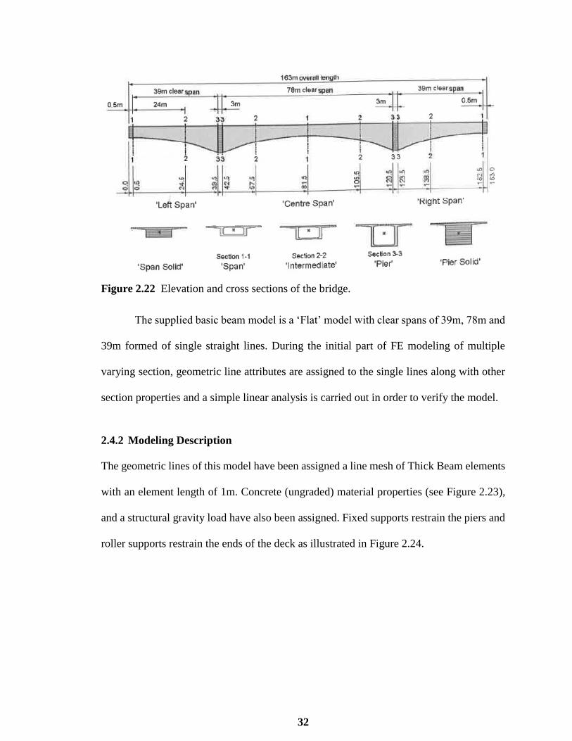
Figure 2.22 Elevation and cross sections of the bridge.
The supplied basic beam model is a ‘Flat’ model with clear spans of 39m, 78m and
39m formed of single straight lines. During the initial part of FE modeling of multiple
varying section, geometric line attributes are assigned to the single lines along with other
section properties and a simple linear analysis is carried out in order to verify the model.
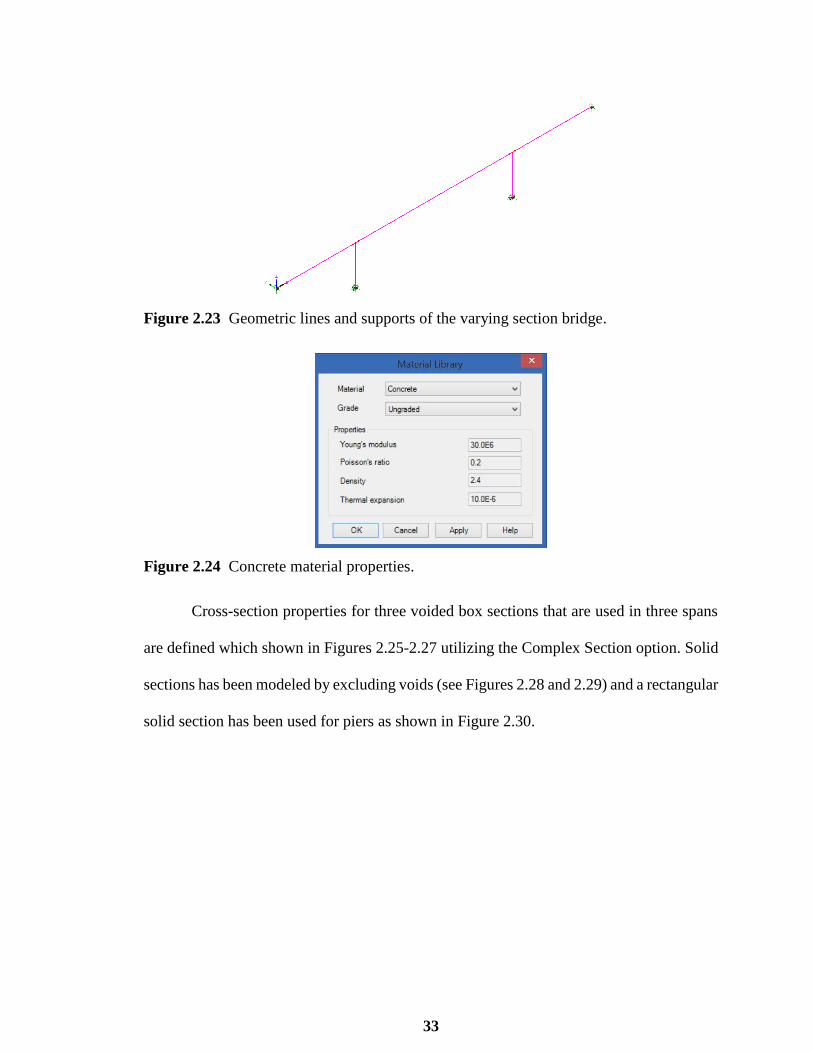
2.4.2 Modeling Description
The geometric lines of this model have been assigned a line mesh of Thick Beam elements
with an element length of 1m. Concrete (ungraded) material properties (see Figure 2.23),
and a structural gravity load have also been assigned. Fixed supports restrain the piers and
roller supports restrain the ends of the deck as illustrated in Figure 2.24.
33
Figure 2.23 Geometric lines and supports of the varying section bridge.
Figure 2.24 Concrete material properties.
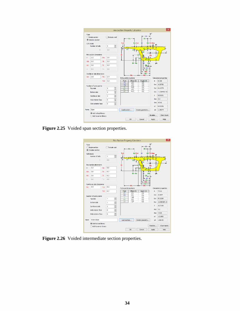
Cross-section properties for three voided box sections that are used in three spans
are defined which shown in Figures 2.25-2.27 utilizing the Complex Section option. Solid
sections has been modeled by excluding voids (see Figures 2.28 and 2.29) and a rectangular
solid section has been used for piers as shown in Figure 2.30.
34
Figure 2.25 Voided span section properties.
Figure 2.26 Voided intermediate section properties.

35
Figure 2.27 Properties of the voided section adjacent to the pier.
Figure 2.28 Solid span section properties.

36
Figure 2.29 Solid pier section properties.
Figure 2.30 Column section properties.
37
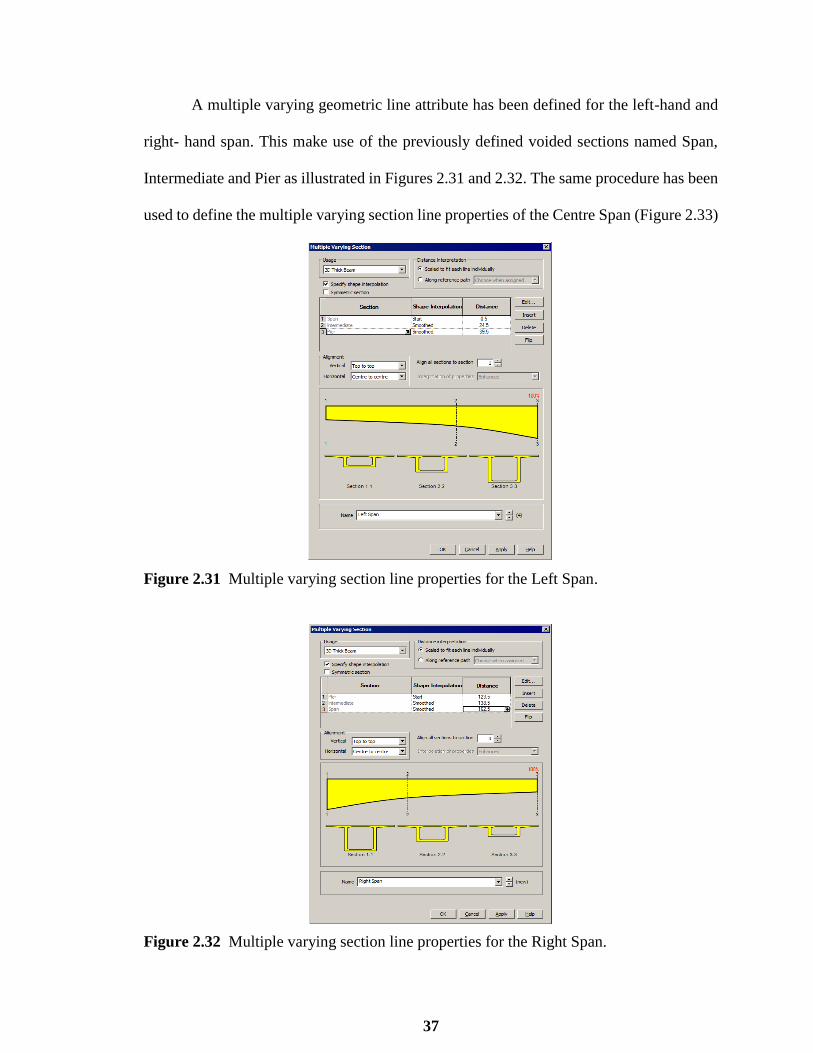
A multiple varying geometric line attribute has been defined for the left-hand and
right- hand span. This make use of the previously defined voided sections named Span,
Intermediate and Pier as illustrated in Figures 2.31 and 2.32. The same procedure has been
used to define the multiple varying section line properties of the Centre Span (Figure 2.33)
Figure 2.31 Multiple varying section line properties for the Left Span.
Figure 2.32 Multiple varying section line properties for the Right Span.

38
Figure 2.33 Multiple varying section line properties for the Centre Span.
The damage bridge model has been defined using the same procedure. Depth of the
box section has been decreased as illustrated in Figure 2.35 at four locations before and
after each pier (see Figure 2.35) representing the damage in order to investigate its effect
on modal parameters.
Figure 2.34 Damaged section properties.

39
Figure 2.35 Location of the damage.
2.4.3 Moving Load Analysis
In the first step, Eigenvalue controls are defined as properties of the loadcase as presented
in Figure 2.36.
Figure 2.36 Eigenvalue controls.
Afterwards, moving load calculations are performed using the IMDPlus facility. In
order to carry out the moving load analysis of the truck travelling across the following three
stages have been carried out:
Defining the path along which the moving loads travel. For this bridge the unit axle
load has been defined as a discrete point load called Unit Axle Load which defines
the unit loading from a single axle of AASHTO LRFD design Truck (HS-20)
(Figure 2.37) and acts vertically.
40
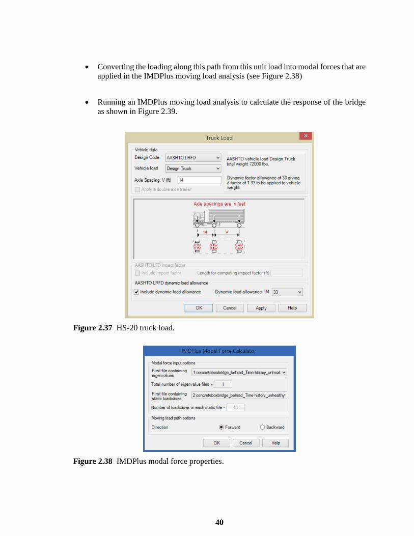
Converting the loading along this path from this unit load into modal forces that are
applied in the IMDPlus moving load analysis (see Figure 2.38)
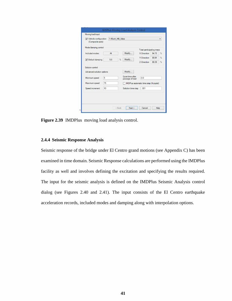
Running an IMDPlus moving load analysis to calculate the response of the bridge
as shown in Figure 2.39.
Figure 2.37 HS-20 truck load.
Figure 2.38 IMDPlus modal force properties.
41
`
Figure 2.39 IMDPlus moving load analysis control.
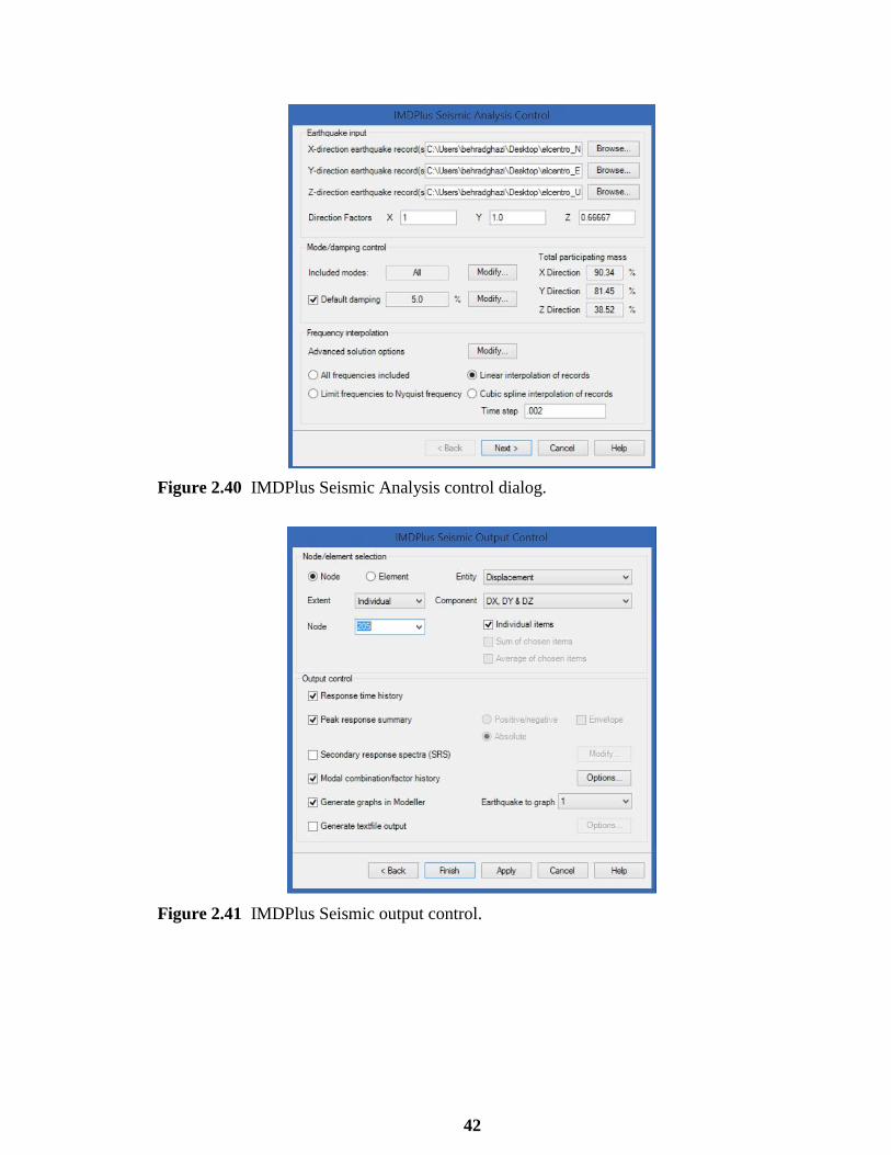
2.4.4 Seismic Response Analysis
Seismic response of the bridge under El Centro grand motions (see Appendix C) has been
examined in time domain. Seismic Response calculations are performed using the IMDPlus
facility as well and involves defining the excitation and specifying the results required.
The input for the seismic analysis is defined on the IMDPlus Seismic Analysis control
dialog (see Figures 2.40 and 2.41). The input consists of the El Centro earthquake
acceleration records, included modes and damping along with interpolation options.
42
Figure 2.40 IMDPlus Seismic Analysis control dialog.
Figure 2.41 IMDPlus Seismic output control.

43
2.4.5 Natural Frequency Analysis Results
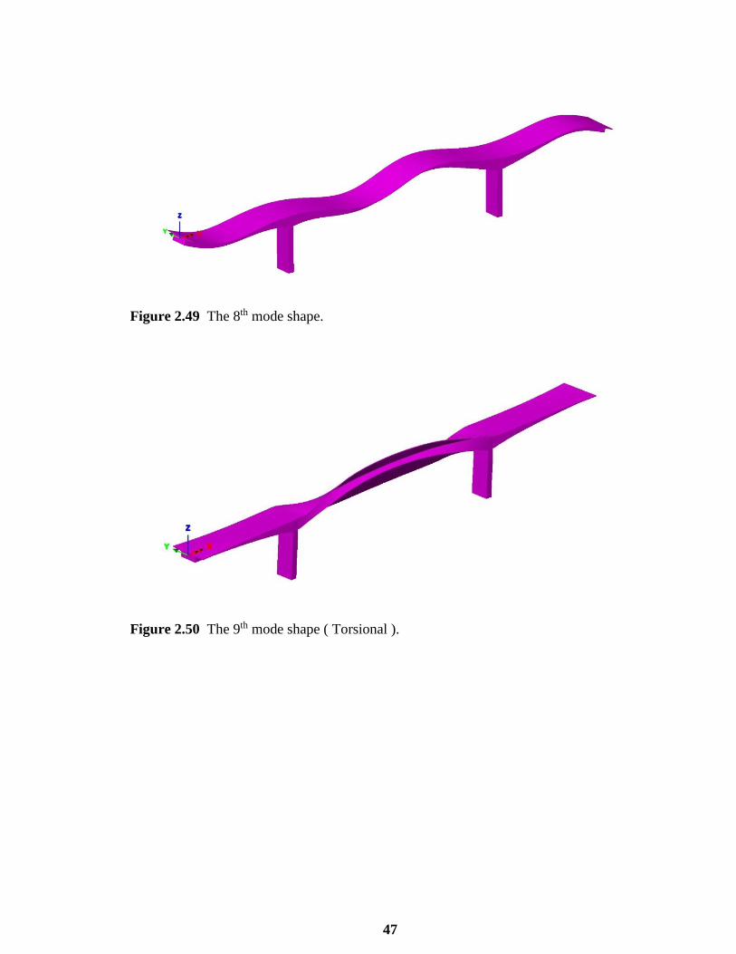
The first 10 mode shapes obtained from eigenvalue frequency analysis are presented in
Figures 2.42-2.51. The first, third, fourth, seventh and tenth vibrational modes are
transverse modes. The second fifth, sixth and eighth modes are vertical modes and Ninth
mode is torsional (see Figure 2.50). Eigenvalue results of the first 10 mode shapes for the
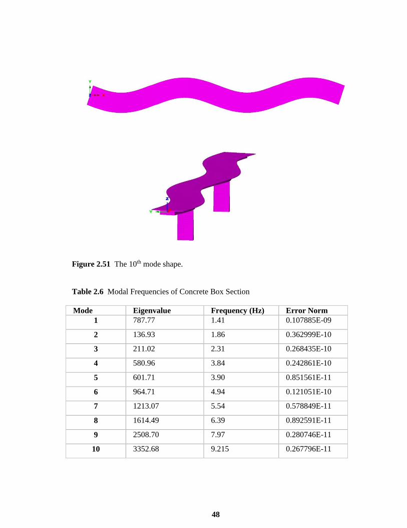
whole structure are displayed in Table 2.6. Noting that the frequency in Hertz is obtained
by dividing the square root of the eigenvalue by 2, and the period of vibration in seconds
can be obtained using the reciprocal of frequency (1/frequency). The error norm for a given
mode provides a relative measure of the accuracy of the computed modes. A high error
norm signifies inaccuracy in either the eigenvalue or the eigenvector, or both and will
provoke a warning message in Lusas Bridge software.
Figure 2.42 The 1st mode shape (frequency: 1.41 Hz).

44
Figure 2.43 The 2nd mode shape (frequency: 1.86 Hz).
Figure 2.44 The 3rd mode shape, plan view on top and 3D view at the bottom (frequency:
2.31 Hz).

45
Figure 2.45 The 4th mode shape, plan view on top and 3D view at the bottom.
Figure 2.46 The 5th mode shape.

46
Figure 2.47 The 6th mode shape.
Figure 2.48 The 7th mode shape, plan view on top and 3D view at the bottom .
47
Figure 2.49 The 8th mode shape.
Figure 2.50 The 9th mode shape ( Torsional ).
48
Figure 2.51 The 10th mode shape.
Table 2.6 Modal Frequencies of Concrete Box Section
Mode Eigenvalue Frequency (Hz) Error Norm
1 787.77 1.41 0.107885E-09
2 136.93 1.86 0.362999E-10
3 211.02 2.31 0.268435E-10
4 580.96 3.84 0.242861E-10
5 601.71 3.90 0.851561E-11
6 964.71 4.94 0.121051E-10
7 1213.07 5.54 0.578849E-11
8 1614.49 6.39 0.892591E-11
9 2508.70 7.97 0.280746E-11
10 3352.68 9.215 0.267796E-11

49
2.4.6 Moving Load Analysis Results
Initially Moving Load Analysis has been carried out by moving the HS-20 truck over the
bridge and the response of the mid-span of the bridge for the range of speeds selected is
investigated. The displacements of the mid-span for a single speed of 15 m/s (or 54 kph) is
presented in Figure 2.52. The vertical acceleration response of the mid-span for the same
truck speed shown in Figure 2.53.
Figure 2.52 Displacement time history of the mid-span for truck speed of 15 m/s,
Displacement (meter) & Time (Seconds).
Figure 2.53 Acceleration of the mid-span for truck speed of 15 m/s, Acceleration (𝑚/𝑠2)
& Time (Seconds).

50
Previously, the displacement and acceleration response of the mid-span of the
bridge deck for a single truck speed are illustrated. Now the peak positive and negative
vertical displacement and acceleration responses of the mid-span over the speed range of
15 m/s to 75 m/s as specified previously in the moving load analysis control dialog will be
shown in Figures 2.54 and 2.55.
Figure 2.54 Peak vertical displacement response of the mid-span over the speed range of
15 m/s to 75 m/s, Displacement (meter).
Figure 2.55 Peak vertical acceleration response of the mid-span over the speed range of
15 m/s to 75 m/s, Acceleration (𝑚/𝑠2).
51
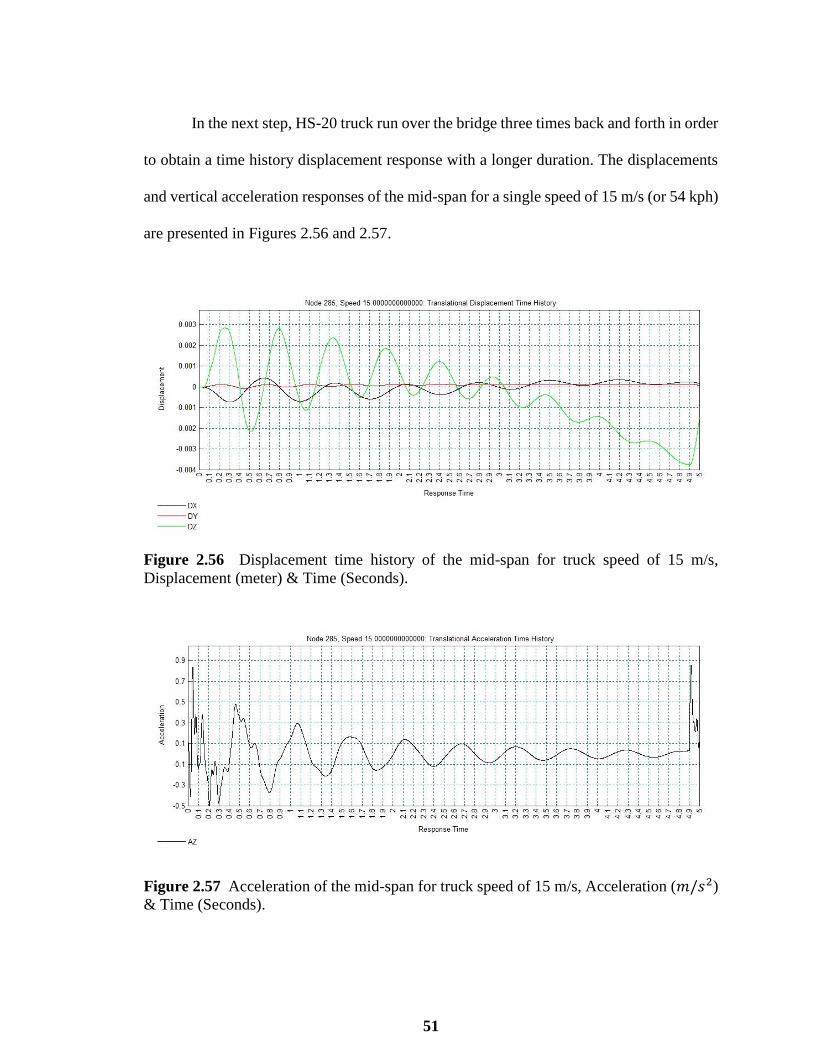
In the next step, HS-20 truck run over the bridge three times back and forth in order
to obtain a time history displacement response with a longer duration. The displacements
and vertical acceleration responses of the mid-span for a single speed of 15 m/s (or 54 kph)
are presented in Figures 2.56 and 2.57.
Figure 2.56 Displacement time history of the mid-span for truck speed of 15 m/s,
Displacement (meter) & Time (Seconds).
Figure 2.57 Acceleration of the mid-span for truck speed of 15 m/s, Acceleration (𝑚/𝑠2)
& Time (Seconds).
52
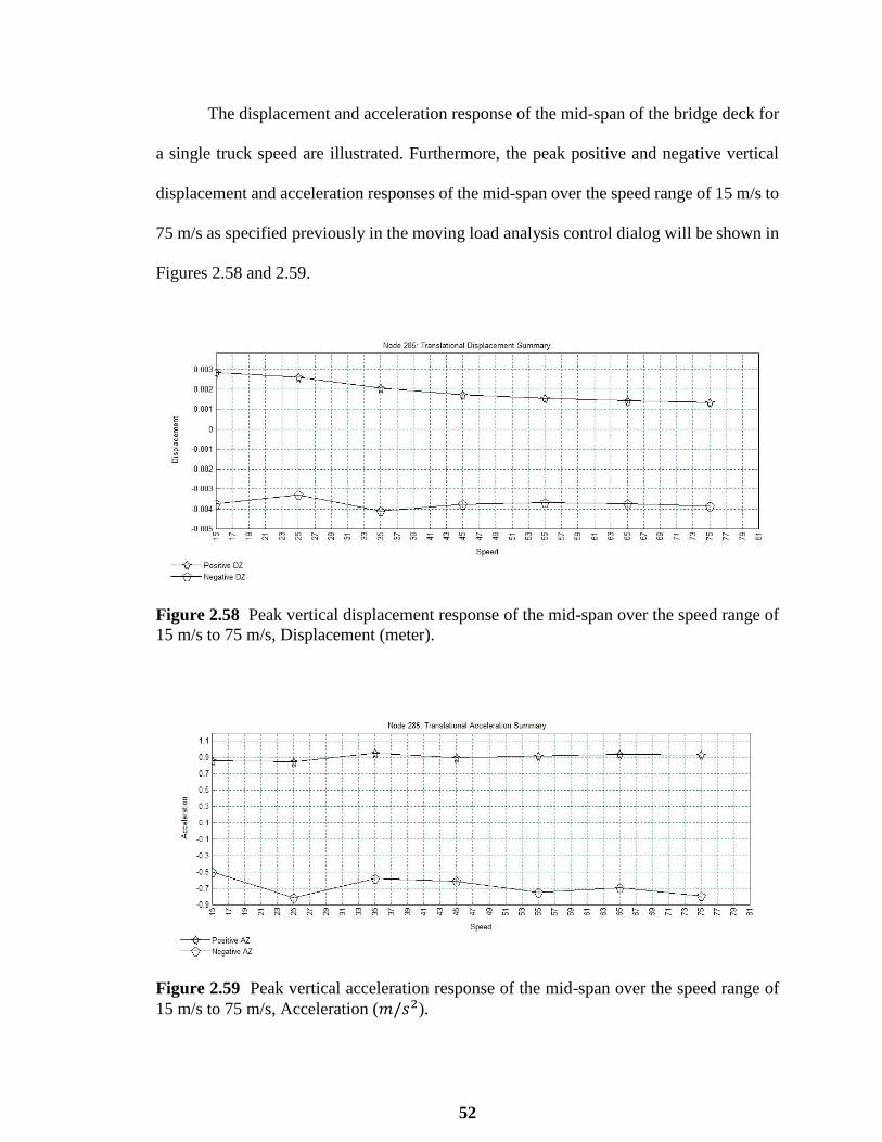
The displacement and acceleration response of the mid-span of the bridge deck for
a single truck speed are illustrated. Furthermore, the peak positive and negative vertical
displacement and acceleration responses of the mid-span over the speed range of 15 m/s to
75 m/s as specified previously in the moving load analysis control dialog will be shown in
Figures 2.58 and 2.59.
Figure 2.58 Peak vertical displacement response of the mid-span over the speed range of
15 m/s to 75 m/s, Displacement (meter).
Figure 2.59 Peak vertical acceleration response of the mid-span over the speed range of
15 m/s to 75 m/s, Acceleration (𝑚/𝑠2).

53
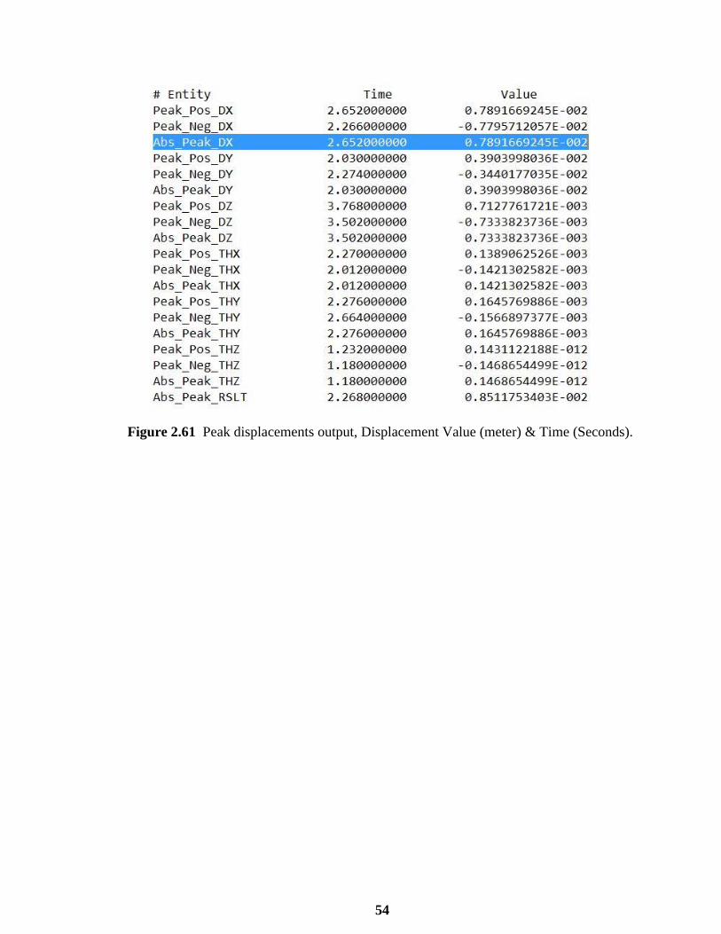
2.4.7 Seismic Response Analysis Results
Seismic Response of the bridge under El Centro earthquake ground motion is presented in
this section. The displacement of the mid-span of the bridge deck has been shown in Figure
2.60. Peak displacements are also output to Notepad and indicate absolute peak
displacements of 0.0079 m in the X-direction, 0.0039 m in the Y-direction along with
additional output for the Z-direction and rotations about each of these axes as presented in
Figure 2.61. From this output we can identify times of 2.652 seconds and 2.03 seconds
which correspond to the absolute peak displacements in the X and Y directions
respectively.
Figure 2.60 Displacement time history of the mid-span under El Centro earthquake,
Displacement (meter) & Time (Seconds).
54
Figure 2.61 Peak displacements output, Displacement Value (meter) & Time (Seconds).

55
2.5 Analysis of 6-Span Precast Segmental Box Girder Bridge
2.5.1 Description of the Bridge
The investigated structure is a six-span precast segmental box girder bridge with a total
length of approximately 250 m (820 ft.) and a width of 12.30 m (40 ft.). It carries two east-
bound and two west-bound lanes. The bridge is located in Qatar. Figure 2.62 provides an
aerial view of the bridge site and Figure 2.63 shows a side view of the bridge structure.
The superstructure consists of a post-tensioned concrete box girder system with three
central spans of 46 m each, 1 central span of 40 m and two shorter end spans of 37 m and
34 m. Thickness of the deck and sections heights are respectively 0.25m and 2.00m with
50mm wearing surface, as shown in Figure 2.64.
Figure 2.62 Aerial Photo of the bridge.
The substructure consists of five column piers and two stub abutments. Concrete
with compressive strength of 25 Mpa (3600 psi) and 20 Mpa (3000 psi) used for piers and
foundation. Mechanically Stabilized Earth (MSE) walls were used behind the existing

56
abutments because of poor soil conditions. The MSE walls are supported on 1.00 m
diameter cast in place concrete piles with design capacity of 4500 kN and rested on
bedrock. All existing pier piles have been driven vertically. From both ends, abutments
separate the bridge from the road approach with expansion joints. The box-girder system
is resting on elastomeric bearings. Piers 2 and 3 have fixed bearings, while sliding guided
bearings are used for the rest of piers and abutments. Rotation of bearings are less than
0.02 (Rad.) for both longitudinal and transverse directions. All the Foundations were
designed to a net allowable bearing pressure of 600 kN/𝑚2. The bridge crosses Qatar
Expressway on 15 degrees skewed alignment. A concrete parapet with a bridge railing and
sound wall is placed along the south edge of the bridge. The bridge was opened for traffic
in 2011.
Figure 2.63 Side view of the bridge.
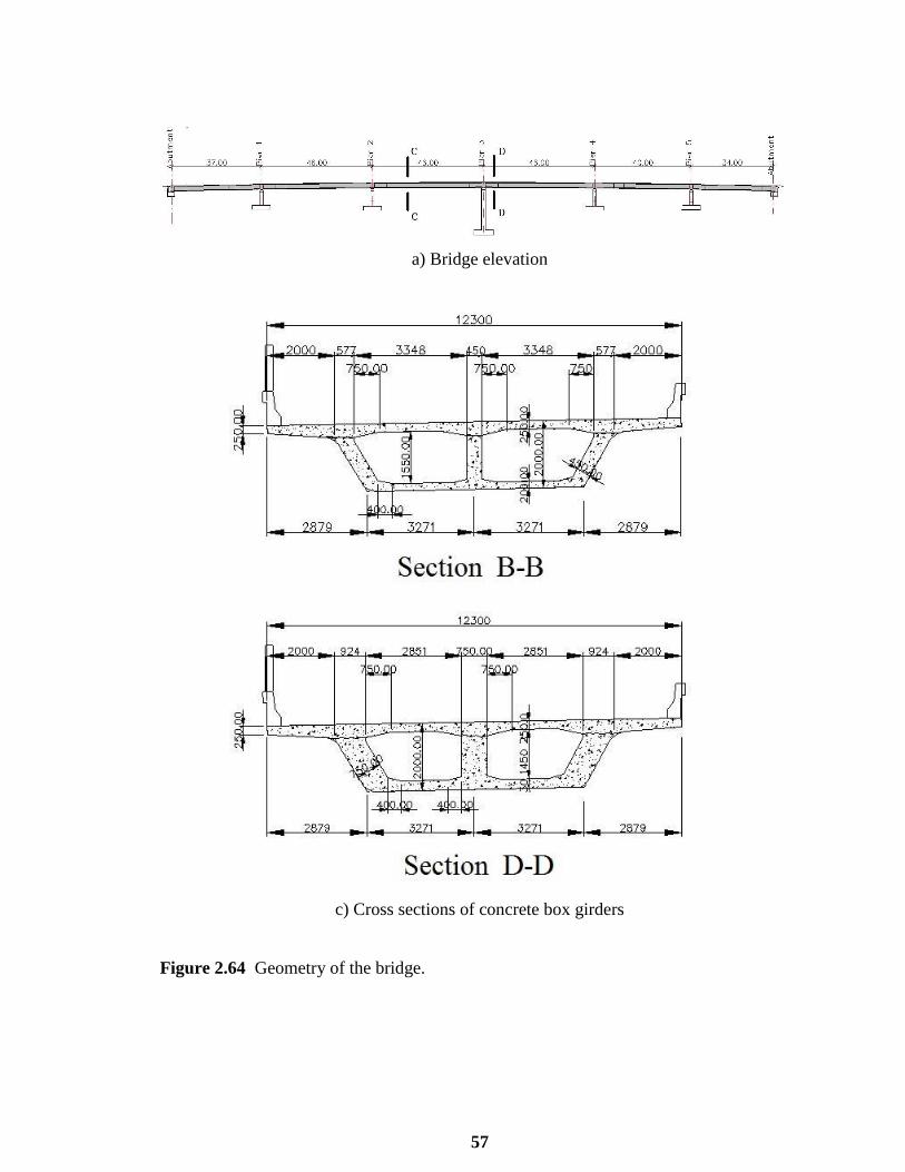
57
a) Bridge elevation
c) Cross sections of concrete box girders
Figure 2.64 Geometry of the bridge.

58
2.5.2 Modeling Description
A complete analysis using Lusas Bridge software requires a description of the material, the
model configuration, boundary conditions, and loading. For service-load simulations, at
least two material constants are required to characterize the linear elastic behavior of the
material:Young’s modulus (E) and Poisson’s ratio (). For nonlinear analysis, the steel and
concrete uniaxial behaviors beyond the elastic range must be defined to simulate their
behavior at higher stresses. The minimum input parameters required to define the concrete
material are the uniaxial compression curve, the ratio of biaxial and uniaxial compressive
strength, and the uniaxial tensile strength. Lusas is equipped with default values if
necessary, which are indicative of typical concrete performance. Boundary conditions that
represent structural supports specify values of displacement and rotation variables at
appropriate nodes.
The bridge Finite Element model has been completed by employing all of the finite
element strategies discussed in earlier sections. Despite the fact that experimental data were
not yet available for comparison, it was useful to complete a model and conduct a detailed
analysis for such a configuration. The features involved included the following procedures.
2.5.3 Geometry
The 6-Span Precast Segmental Box Girder Bridge is modelled using the box section
property calculator and the multiple varying sections facilities in LUSAS (Figure 2.65).
Units used are kN, m, kg, s, C throughout.
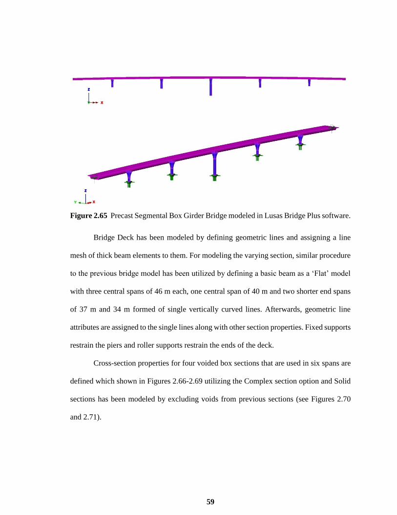
59
Figure 2.65 Precast Segmental Box Girder Bridge modeled in Lusas Bridge Plus software.
Bridge Deck has been modeled by defining geometric lines and assigning a line
mesh of thick beam elements to them. For modeling the varying section, similar procedure
to the previous bridge model has been utilized by defining a basic beam as a ‘Flat’ model
with three central spans of 46 m each, one central span of 40 m and two shorter end spans
of 37 m and 34 m formed of single vertically curved lines. Afterwards, geometric line
attributes are assigned to the single lines along with other section properties. Fixed supports
restrain the piers and roller supports restrain the ends of the deck.
Cross-section properties for four voided box sections that are used in six spans are
defined which shown in Figures 2.66-2.69 utilizing the Complex section option and Solid
sections has been modeled by excluding voids from previous sections (see Figures 2.70
and 2.71).
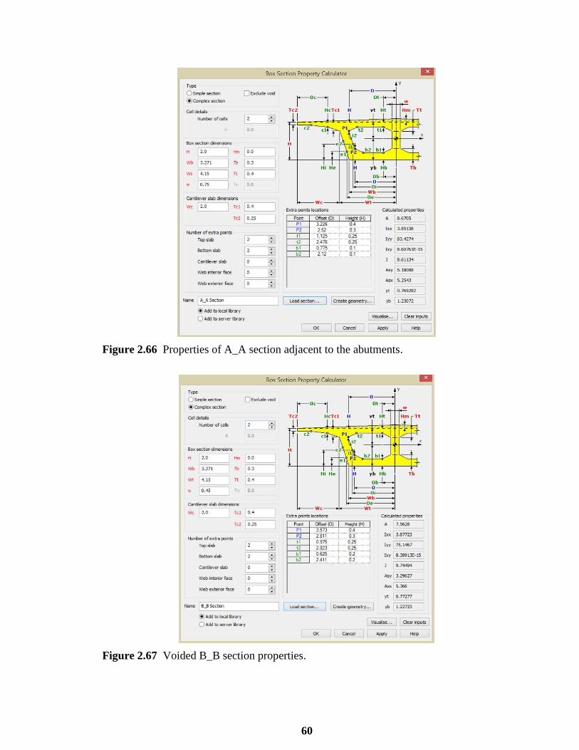
60
Figure 2.66 Properties of A_A section adjacent to the abutments.
Figure 2.67 Voided B_B section properties.
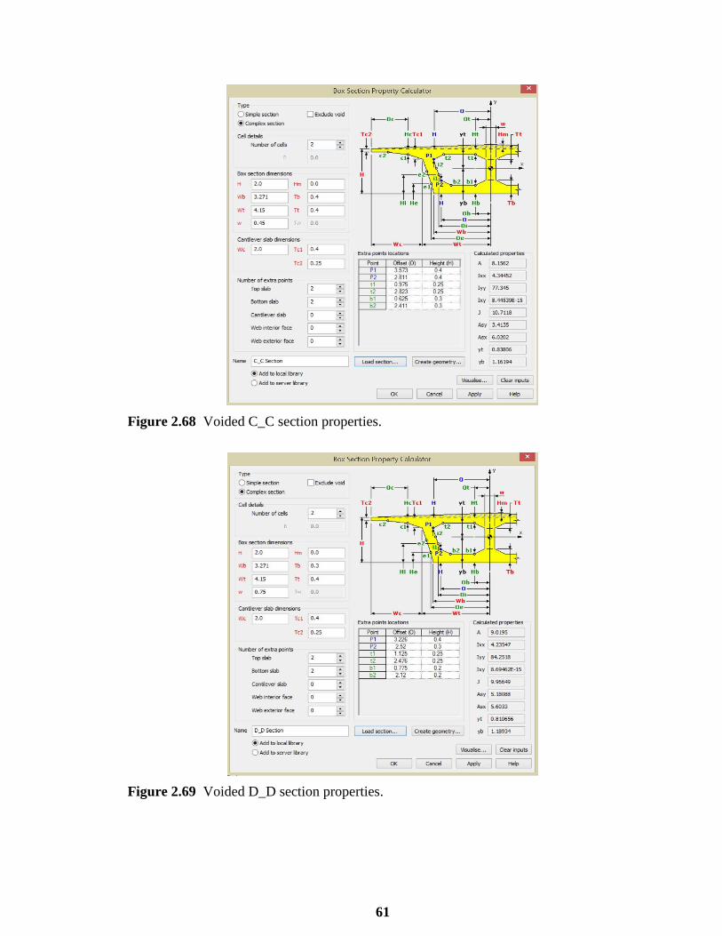
61
Figure 2.68 Voided C_C section properties.
Figure 2.69 Voided D_D section properties.
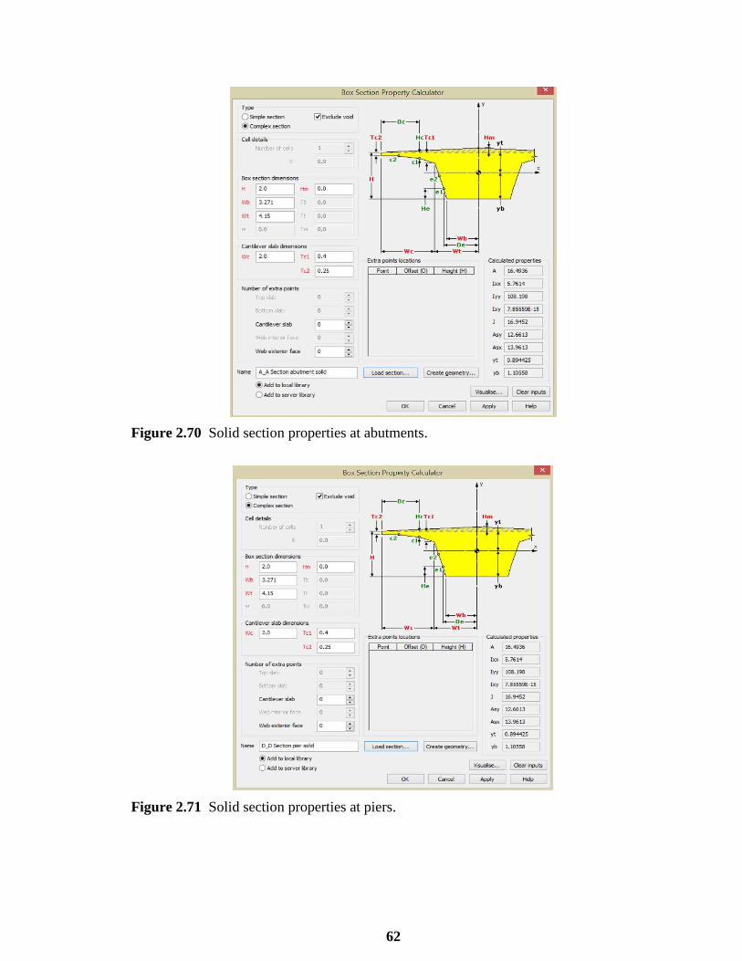
62
Figure 2.70 Solid section properties at abutments.
Figure 2.71 Solid section properties at piers.
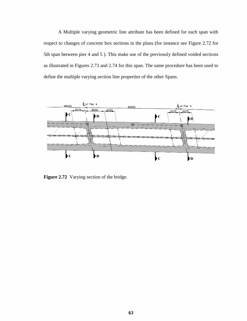
63
A Multiple varying geometric line attribute has been defined for each span with
respect to changes of concrete box sections in the plans (for instance see Figure 2.72 for
5th span between pier 4 and 5 ). This make use of the previously defined voided sections
as illustrated in Figures 2.73 and 2.74 for this span. The same procedure has been used to
define the multiple varying section line properties of the other Spans.
Figure 2.72 Varying section of the bridge.
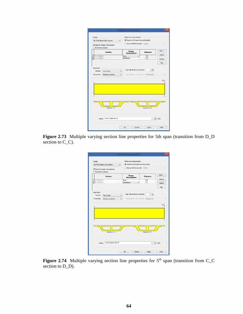
64
Figure 2.73 Multiple varying section line properties for 5th span (transition from D_D
section to C_C).
Figure 2.74 Multiple varying section line properties for 5th span (transition from C_C
section to D_D).
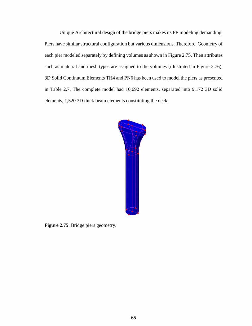
65
Unique Architectural design of the bridge piers makes its FE modeling demanding.
Piers have similar structural configuration but various dimensions. Therefore, Geometry of
each pier modeled separately by defining volumes as shown in Figure 2.75. Then attributes
such as material and mesh types are assigned to the volumes (illustrated in Figure 2.76).
3D Solid Continuum Elements TH4 and PN6 has been used to model the piers as presented
in Table 2.7. The complete model had 10,692 elements, separated into 9,172 3D solid
elements, 1,520 3D thick beam elements constituting the deck.
Figure 2.75 Bridge piers geometry.
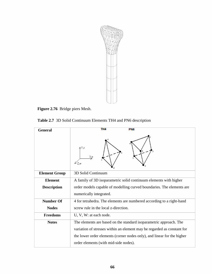
66
Figure 2.76 Bridge piers Mesh.
Table 2.7 3D Solid Continuum Elements TH4 and PN6 description
General
Element Group 3D Solid Continuum
Element
Description
A family of 3D isoparametric solid continuum elements with higher
order models capable of modelling curved boundaries. The elements are
numerically integrated.
Number Of
Nodes
4 for tetrahedra. The elements are numbered according to a right-hand
screw rule in the local z-direction.
Freedoms U, V, W: at each node.
Notes The elements are based on the standard isoparametric approach. The
variation of stresses within an element may be regarded as constant for
the lower order elements (corner nodes only), and linear for the higher
order elements (with mid-side nodes).

67
2.5.4 Material
Development of a model for the behavior of concrete is a challenging task. Concrete is a
quasi-brittle material and has different behavior in compression and tension. The tensile
strength of concrete is typically 8-15% of the compressive strength [20]. Figure 2.77 shows
a typical stress-strain curve for normal weight concrete [21].
Figure 2.77 Typical uniaxial compressive and tensile stress-strain curve for concrete
[21].
In compression, the stress-strain curve for concrete is linearly elastic up to about 30
percent of the maximum compressive strength. Above this point, the stress increases
gradually up to the maximum compressive strength. After it reaches the maximum
compressive strength σcu , the curve descends into a softening region, and eventually
crushing failure occurs at an ultimate strain εcu . In tension, the stress-strain curve for
concrete is approximately linearly elastic up to the maximum tensile strength. After this
point, the concrete cracks and the strength decreases gradually to zero [21].
For concrete, Lusas Bridge software requires input data for material properties as
represented in Figure 2.78.

68
Figure 2.78 Concrete material properties.
2.5.5 Defining the Loads
Three loadcases will be defined Based on AASHTO LRFD specifications:
The self-weight of the bridge.
A Lane load equivalent to a traffic load over the full length and width of the traffic
lane.
A design truck moving load over the full length of the bridge.

69
2.5.5.1 Self-weight The self-weight is defined as a gravity acceleration in the negative
Z direction. The correct units are automatically calculated when the gravity loading is
selected from the bridge menu.
2.5.5.2 Lane Load The second load will represent a lane load along the traffic lanes as
shown in Figures 2.79 and 2.80. In Lusas Bridge Plus software, Vehicle and Lane loads
are represented by Patch loads that are assigned to points which may form part of the
model, or may be defined specifically to locate the bridge loads.
Figure 2.79 AASHTO LRFD design lane load description.
Figure 2.80 AASHTO LRFD design lane load applied to the bridge model.
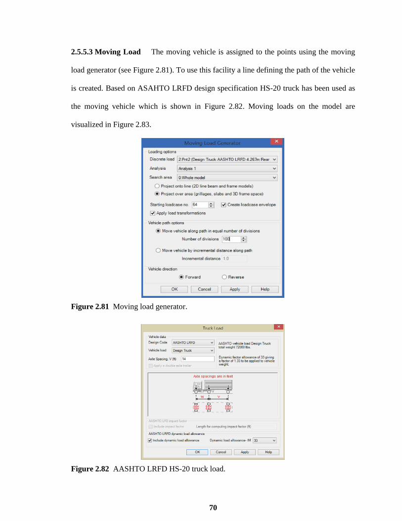
70
2.5.5.3 Moving Load The moving vehicle is assigned to the points using the moving
load generator (see Figure 2.81). To use this facility a line defining the path of the vehicle
is created. Based on ASAHTO LRFD design specification HS-20 truck has been used as
the moving vehicle which is shown in Figure 2.82. Moving loads on the model are
visualized in Figure 2.83.
Figure 2.81 Moving load generator.
Figure 2.82 AASHTO LRFD HS-20 truck load.

71
Figure 2.83 Moving HS-20 truck on the bridge FE model.
In the Last step, Eigenvalue controls are defined as properties of the loadcase.
Figure 2.84 Eigenvalue controls.

72
2.5.6 Analysis Results
Static and Dynamic Finite Element analysis of 6-Span Precast Segmental Box Girder
Bridge has been carried out as presented in the last section. The data show the global
behavior of the bridge model, particularly the distribution of moments and stresses in the
deck. The deformed shape of the bridge under gravity load, AASHTO LRFD design lane
load and HS-20 moving truck have been shown in Figures 2.85-2.87. The bridge has
Maximum deflection of 2cm and 1.9cm under Dead load and Live Load respectively.
Maximum Positive and Negative Displacement Envelope of each node has been illustrated
in Figures 2.88 and 2.89 as the HS-20 truck moves over the bridge.
Figure 2.85 Deformed mesh under gravity Load (max displacement 0.02 m).
Figure 2.86 Deformed mesh under Lane Load (max displacement 0.0018 m).
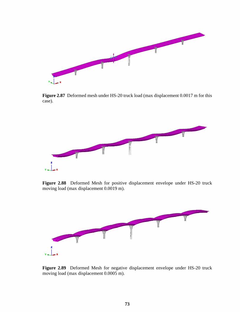
73
Figure 2.87 Deformed mesh under HS-20 truck load (max displacement 0.0017 m for this
case).
Figure 2.88 Deformed Mesh for positive displacement envelope under HS-20 truck
moving load (max displacement 0.0019 m).
Figure 2.89 Deformed Mesh for negative displacement envelope under HS-20 truck
moving load (max displacement 0.0005 m).

74
Furthermore, Moment Diagrams under different Load cases have been shown in
Figures 2.90-2.92. For the case of HS-20 truck moving load, positive and negative Moment
Diagram envelopes have been presented in Figures 2.93 and 2.94. Figures 2.95-2.98
illustrate Stress Contours of the deck and piers as a result of gravity load, lane load and
moving HS-20 truck load applied to the bridge model.
Figure 2.90 Moment Diagram under gravity load (max positive moment 17.47 × 10³
kN.m and max negative moment −35.61 × 10³ kN.m).
Figure 2.91 Moment Diagram under lane load (max positive moment 1.77 × 10³ kN.m
and max negative moment −3.35 × 10³ kN.m).
Figure 2.92 Moment Diagram under HS-20 truck load.
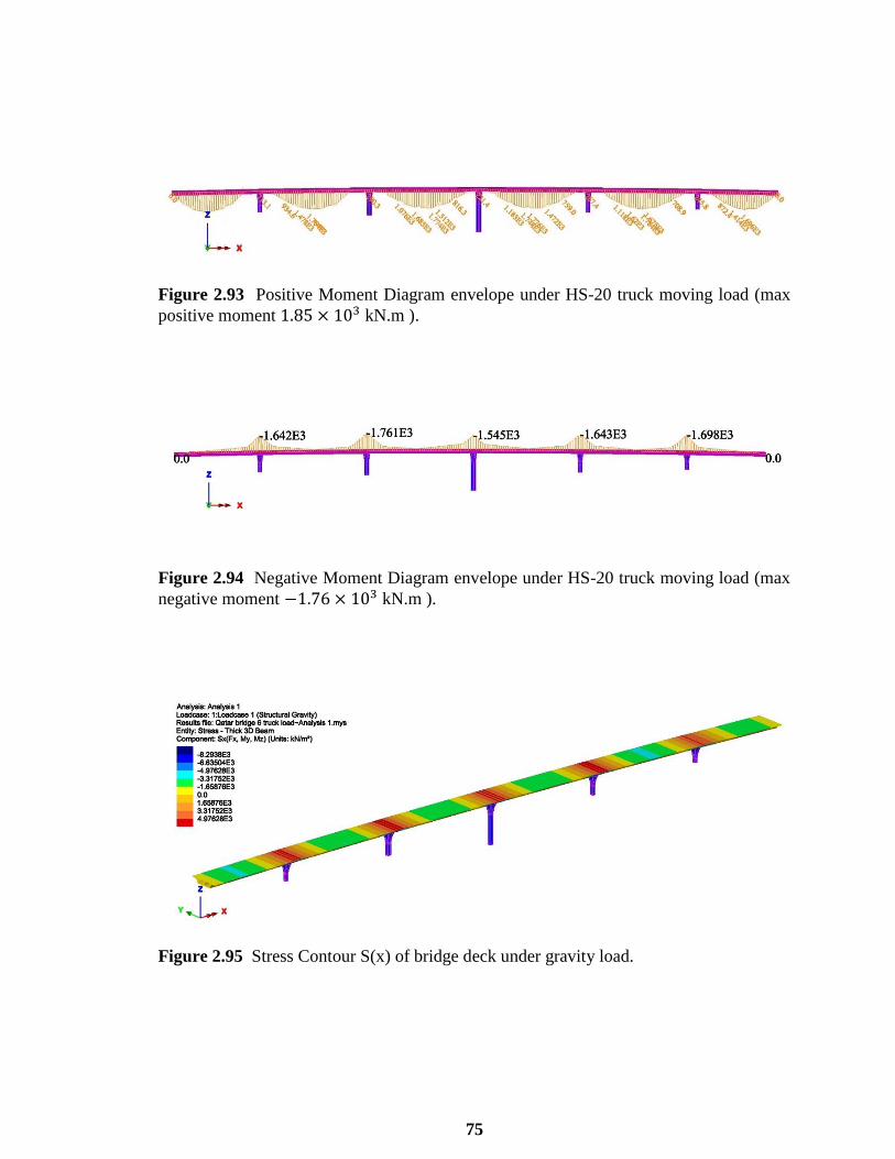
75
Figure 2.93 Positive Moment Diagram envelope under HS-20 truck moving load (max
positive moment 1.85 × 10³ kN.m ).
Figure 2.94 Negative Moment Diagram envelope under HS-20 truck moving load (max
negative moment −1.76 × 10³ kN.m ).
Figure 2.95 Stress Contour S(x) of bridge deck under gravity load.
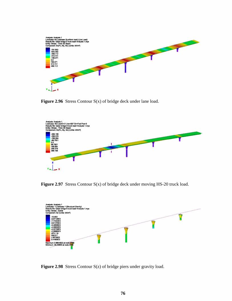
76
Figure 2.96 Stress Contour S(x) of bridge deck under lane load.
Figure 2.97 Stress Contour S(x) of bridge deck under moving HS-20 truck load.
Figure 2.98 Stress Contour S(z) of bridge piers under gravity load.
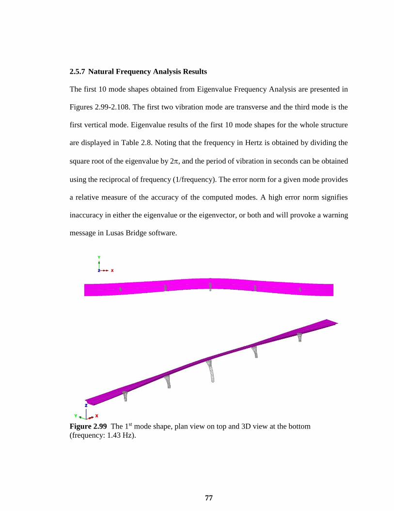
77
2.5.7 Natural Frequency Analysis Results
The first 10 mode shapes obtained from Eigenvalue Frequency Analysis are presented in
Figures 2.99-2.108. The first two vibration mode are transverse and the third mode is the
first vertical mode. Eigenvalue results of the first 10 mode shapes for the whole structure
are displayed in Table 2.8. Noting that the frequency in Hertz is obtained by dividing the
square root of the eigenvalue by 2, and the period of vibration in seconds can be obtained
using the reciprocal of frequency (1/frequency). The error norm for a given mode provides
a relative measure of the accuracy of the computed modes. A high error norm signifies
inaccuracy in either the eigenvalue or the eigenvector, or both and will provoke a warning
message in Lusas Bridge software.
Figure 2.99 The 1st mode shape, plan view on top and 3D view at the bottom
(frequency: 1.43 Hz).
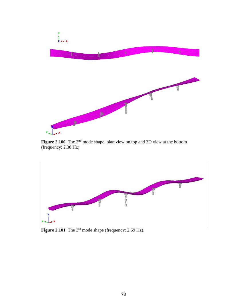
78
Figure 2.100 The 2nd mode shape, plan view on top and 3D view at the bottom
(frequency: 2.38 Hz).
Figure 2.101 The 3rd mode shape (frequency: 2.69 Hz).

79
Figure 2.102 The 4th mode shape.
Figure 2.103 The 5th mode shape.
Figure 2.104 The 6th mode shape, plan view on top and 3D view at the bottom.

80
Figure 2.105 The 7th mode shape.
Figure 2.106 The 8th mode shape.
Figure 2.107 The 9th mode shape.
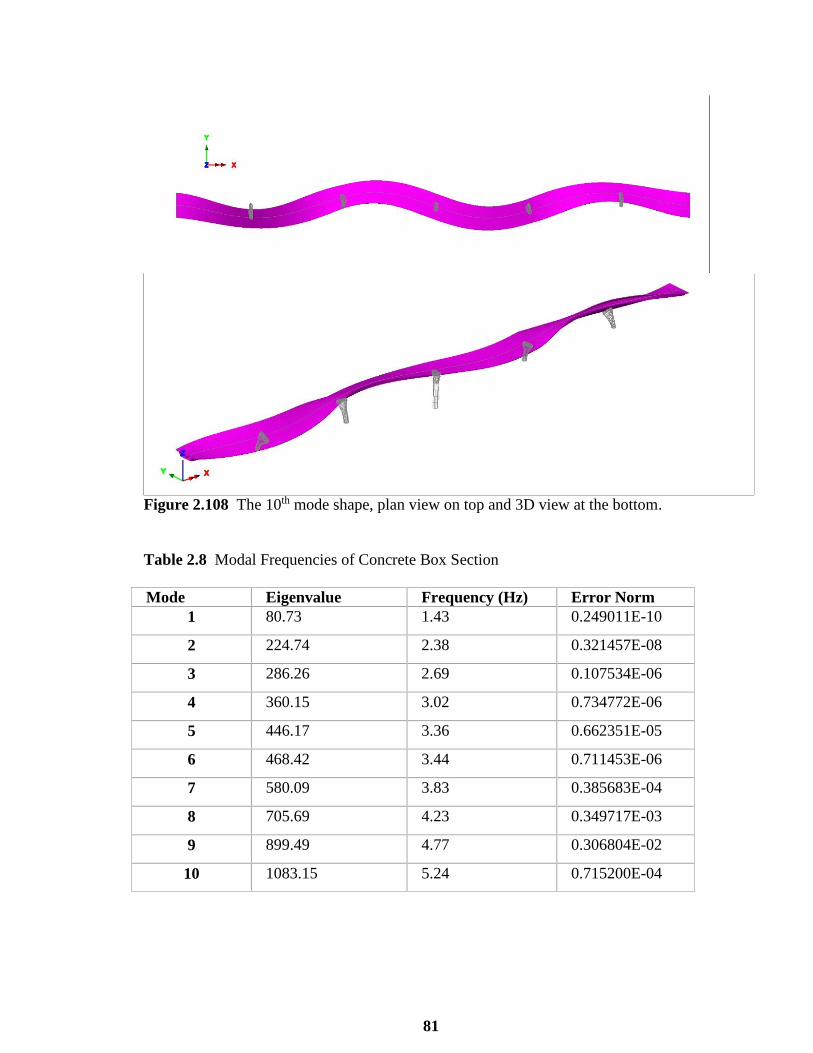
81
Figure 2.108 The 10th mode shape, plan view on top and 3D view at the bottom.
Table 2.8 Modal Frequencies of Concrete Box Section
Mode Eigenvalue Frequency (Hz) Error Norm
1 80.73 1.43 0.249011E-10
2 224.74 2.38 0.321457E-08
3 286.26 2.69 0.107534E-06
4 360.15 3.02 0.734772E-06
5 446.17 3.36 0.662351E-05
6 468.42 3.44 0.711453E-06
7 580.09 3.83 0.385683E-04
8 705.69 4.23 0.349717E-03
9 899.49 4.77 0.306804E-02
10 1083.15 5.24 0.715200E-04

82
2.6 Conclusions
In this chapter, Lusas Bridge plus finite element program was used to simulate the behavior
of an experimental frame, 3-span bridge and the in-service 6-Span Precast Segmental Box
Girder Bridge. In general, the conclusions and methods would be very similar using other
nonlinear Finite Element Analysis programs. Model development for aforementioned
structures is demonstrated. Element types used in the models are covered along with the
constitutive assumptions and parameters for the various materials in each Section. Besides,
Geometry of the models, loading and boundary conditions are illustrated. The mode shapes
obtained from eigenvalue frequency analysis are presented. For the 3-span bridge Moving
Load analysis has been carried using the IMDPlus facility and Seismic response of the
bridge under El Centro earthquake ground motion is presented. Furthermore, Static and
Dynamic Finite Element Analysis of 6-Span Precast Segmental Box Girder Bridge has
been carried out. Finite Element Analysis results for each model thoroughly demonstrated
in each section. The Finite Element Analysis performed in this chapter will be employed
in the next chapters. For future studies, the accuracy of FEA results obtained will be
validated using lab-scale experimental or Structural Health Monitoring results.
Additionally, Finite Element Modal Updating technique can be utilized to obtain calibrated
model of each structure.

83
CHAPTER 3
EXPERIMENTAL WORK
3.1 Introduction
This chapter is dedicated to a preliminary study in designing and setting up a test-bed for
the research on Structural Health Monitoring utilizing Wireless Sensor Networks. To
evaluate the performance of the sensors and validate the proposed optimal design and
algorithms of used wireless sensor network under actual experimental conditions, a series
of tests were carried out on a scaled down frame mounted on the shaking table in the
laboratory. The design and setup of the physical model are presented in detail. Three
different excitation cases has been investigated to evaluate the performance of the
developed wireless sensing system under actual experimental conditions. Furthermore,
responses obtained from the WSN system will be compared to the ones resulted from the
finite element model.
3.2 Reinforced Concrete Frame
Reinforced concrete frame used for this lab experiment was designed by Dr. Mohamed
Mahgoub and constructed in Qatar University Department of Engineering laboratory. The
RC frame is shown in Figure 3.1. The span of the beam is 32.5 cm (12.8 in) and the height
of both columns are 24.5 cm (9.6 in). The frame properties are: The modulus of elasticity
𝐸𝑐 = 31.58MPa (4500 psi), mass per unit volume M = 2400 kg/m3 (150 lb/scf), cross-
section dimensions 5 × 5 cm for an area A = 25 cm2, #2 (6 mm diameter) for Steel rebar,
for stirrups diameter of 3 mm and 1 cm concrete cover. Figure 3.2 shows the frame
dimensions and the location of the rebar. There were four main flexural steel bars extending
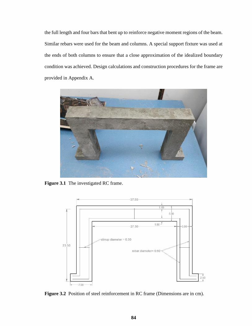
84
the full length and four bars that bent up to reinforce negative moment regions of the beam.
Similar rebars were used for the beam and columns. A special support fixture was used at
the ends of both columns to ensure that a close approximation of the idealized boundary
condition was achieved. Design calculations and construction procedures for the frame are
provided in Appendix A.
Figure 3.1 The investigated RC frame.
Figure 3.2 Position of steel reinforcement in RC frame (Dimensions are in cm).
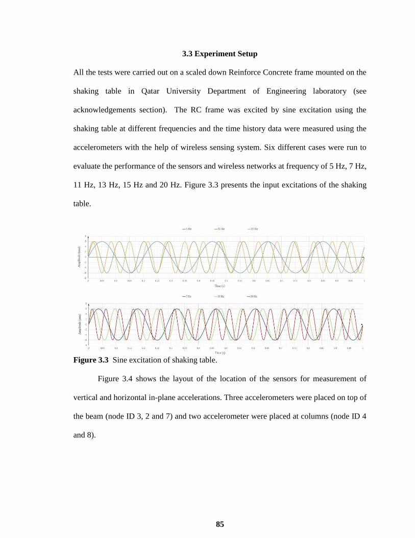
85
3.3 Experiment Setup
All the tests were carried out on a scaled down Reinforce Concrete frame mounted on the
shaking table in Qatar University Department of Engineering laboratory (see
acknowledgements section). The RC frame was excited by sine excitation using the
shaking table at different frequencies and the time history data were measured using the
accelerometers with the help of wireless sensing system. Six different cases were run to
evaluate the performance of the sensors and wireless networks at frequency of 5 Hz, 7 Hz,
11 Hz, 13 Hz, 15 Hz and 20 Hz. Figure 3.3 presents the input excitations of the shaking
table.
Figure 3.3 Sine excitation of shaking table.
Figure 3.4 shows the layout of the location of the sensors for measurement of
vertical and horizontal in-plane accelerations. Three accelerometers were placed on top of
the beam (node ID 3, 2 and 7) and two accelerometer were placed at columns (node ID 4
and 8).
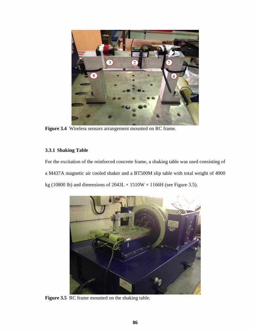
86
Figure 3.4 Wireless sensors arrangement mounted on RC frame.
3.3.1 Shaking Table
For the excitation of the reinforced concrete frame, a shaking table was used consisting of
a M437A magnetic air cooled shaker and a BT500M slip table with total weight of 4900
kg (10800 lb) and dimensions of 2043L × 1510W × 1166H (see Figure 3.5).
Figure 3.5 RC frame mounted on the shaking table.

87
M437A shaker has the capacity of maximum force of 8,800 lbf peak sine force with
a dynamic performance ranging from DC to 2,500 Hz and designed for specimen payload
up to 500 kg (1102 lbs). Other properties of the shaker has been presented in Table 3.1.
The BT500M slip table with the dimensions of 500 mm × 500 mm (19.7 in × 19.7 in) is
capable of providing high over-turning moment and cross-axial restraints, since it
combines a standard slip table assembly with 3,000 psi hydrostatic bearings to provide high
dynamic moment restraint while preserving the damping characteristics of an oil film.
Additionally, light weight magnesium has been used for the slip plate (see Table 3.2 for
more details). As shown in Figure 3.5, the frame is mounted on the shaking table using
fully threaded stainless steel bolts.
Table 3.1 M437A Shaker Properties
System Performance American Metric
Sine Force 8,800 lbf 4,000 kgf
Shock Force (6ms) 17,600 lbf 8,000 kgf
Useful Frequency Range DC to 2,500 Hz DC to 2,500 Hz
Continuous Displacement 2.0 in 51 mm
Max Velocity 5.9 ft/s 1.8 m/s
Max Acceleration (sine) 100 g 981 m/s²
Max Static Payload 1102 lb 500 kg
Armature Diameter 14.5 in 370 mm
Armature Material Aluminum (A) Aluminum (A)
Amplifier Series/Model Number MPA409 MPA409

88
Table 3.2 BT500M Slip Table Properties
System Performance American Metric
Slip Plate Working Surface 19.7 x 19.7 in 500 x 500 mm
Slip Plate Material Magnesium (M) Magnesium (M)
Slip Plate Thickness 1.57 in 40 mm
Slip Plate Grid plus amature pattern 4 in grid 100 mm grid
Slip Plate Mass 46.2 lb 21 kg
Max Payload 882 lb 400 kg
3.3.2 Measurement Sensors
Regarding the wireless based equipment, the Crossbow technology [22] was chosen as it
offers economical solutions including low powering boards and measurement platforms
with microaccelerometers embedded. The selected Crossbow product (WSN professional
kit) uses as gateway a IRIS Mote board (Figure 3.6) in charge of the communication over
the network in the radio frequency range of 2.4 to 2.48 GHz. IRIS Mote provides three
times radio range and twice the program memory over previous MICA Motes and Outdoor
line-of-sight tests have yielded ranges as far as 500 meters between nodes without
amplification. Additionally, any IRIS Mote can function as a base station when it is
connected to a standard PC interface or gateway board. A base station allows the
aggregation of sensor network data onto a PC or other computer platform.
Figure 3.6 IRIS mote board top and bottom view.

89
To provide communication, in-system programming and to supply energy to the
devices, the system uses an interface board model MIB520 (Figure 3.6) connected to a
central computer trough an USB bus. USB Bus power eliminates the need for an external
power source for this board.
Figure 3.7 MIB520 USB interface board.
The sensors’ platform supplied by Crossbow is composed by a measurement board
that works mounted on an IRIS Mote board. In this unit, the IRIS Mote board is not only
in charge of the network communication but also in charge of supplying energy to the
measurement board (using two AA batteries), as well as acquiring and converting the
analog measurements with an ADC resolution of 10 bits. There are several options of
measurements boards available in the market, however; the one suitable for dynamic
monitoring works is the MTS400 which developed in conjunction with UC Berkeley and
Intel Research Labs. This measurement board has embedded four microsensors: biaxial
microaccelerometer; light; pressure-temperature; and humidity-temperature. Table 3.3
presents the characteristics of the biaxial microaccelerometer ADXL202 embedded in the
MTS400 board. These sensor boards utilize the latest generation of IC-based surface mount
sensors which enable these energy-efficient digital devices to provide extended battery-life
and performance wherever low maintenance field-deployed sensor nodes are required. The
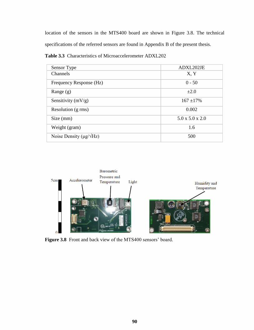
90
location of the sensors in the MTS400 board are shown in Figure 3.8. The technical
specifications of the referred sensors are found in Appendix B of the present thesis.
Table 3.3 Characteristics of Microaccelerometer ADXL202
Sensor Type ADXL202JE
Channels X, Y
Frequency Response (Hz) 0 - 50
Range (g) ±2.0
Sensitivity (mV/g) 167 ±17%
Resolution (g rms) 0.002
Size (mm) 5.0 x 5.0 x 2.0
Weight (gram) 1.6
Noise Density (μg/√Hz) 500
Figure 3.8 Front and back view of the MTS400 sensors’ board.
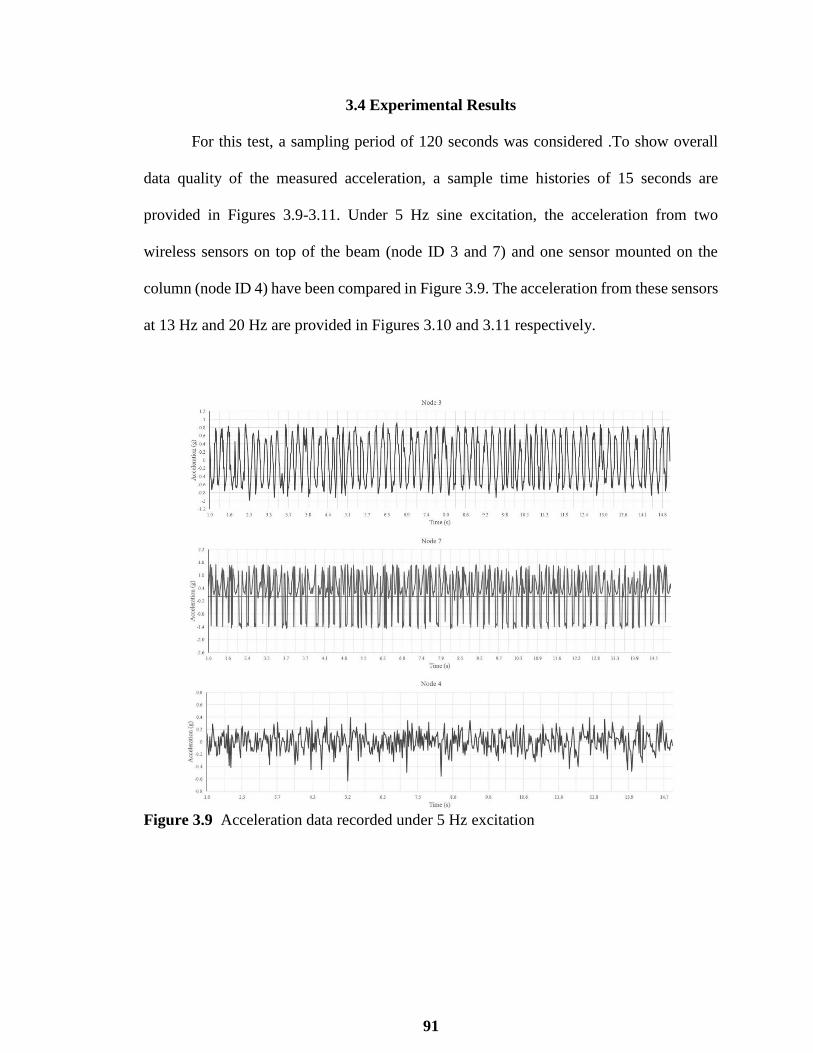
91
3.4 Experimental Results
For this test, a sampling period of 120 seconds was considered .To show overall
data quality of the measured acceleration, a sample time histories of 15 seconds are
provided in Figures 3.9-3.11. Under 5 Hz sine excitation, the acceleration from two
wireless sensors on top of the beam (node ID 3 and 7) and one sensor mounted on the
column (node ID 4) have been compared in Figure 3.9. The acceleration from these sensors
at 13 Hz and 20 Hz are provided in Figures 3.10 and 3.11 respectively.
Figure 3.9 Acceleration data recorded under 5 Hz excitation
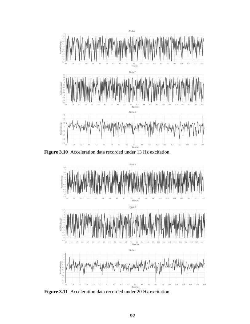
92
Figure 3.10 Acceleration data recorded under 13 Hz excitation.
Figure 3.11 Acceleration data recorded under 20 Hz excitation.

93
From the experimental data it can be observed that the accelerations measured seem
identical to the excitation due to the fact that the frame with the small size being very rigid.
Moreover, for all excitation cases the recordings of the three accelerometers are very
similar because of the geometric size of the RC frame model.
3.5 Conclusions
This chapter presents a preliminary study in designing and setting up a test-bed for the
research on SHM of bridges utilizing Wireless Sensor Networks. The test-bed encompasses
the physical model and FE model of a scaled down reinforced concrete frame. The design
and setup of the physical model are presented in detail.
The Reinforced Concrete frame was excited by sine excitation using the shaking
table at six different frequencies and the time history data were measured using five MEMS
accelerometers with the help of wireless sensing system. Note that the problems related to
the energy consumption were not considered since the use of these platforms for long term
monitoring was outside the scope of these tests. Time histories of the measured
accelerations are provided at three different frequency. In conclusion, the plot results show
that the developed wireless sensing system is capable of measuring the dynamic response
of the RC frame structure with reliable precision level.
In the future studies, dynamic characterization of the RC frame will be carried out
to determine the modal properties of the frame such as: natural frequencies, modal shapes
and damping ratios. Subsequently, the natural frequencies and mode shapes obtained from
the initial FE model in Section 2.3 will be compared with those measured from the vibration
tests. Finite Element Model updating is needed to improve the FE model, Hence, these

94
measured dynamic characteristics of the physical model will be used for updating the FE
model of the RC frame. Eventually, damage cases will be applied in the frame in the form
of saw cuts perpendicular to the longitudinal axis of the beam. Modal test results obtained
from the damaged frame will be compared to the updated FE model for the subsequent
studies of damage detection.

95
CHAPTER 4
IMPLEMENTATION OF HEALTH MONITORING SYSTEM ON
AN IN-SERVICE HIGHWAY BRIDGE
4.1 Introduction
Major applications of SHM have been implemented in the oil industry, large dams and
bridges and have acquired a great deal of research and practical efforts. Residential and
commercial structures have received relatively little attention in comparison [10]. Bridge
monitoring can be dated back to the construction of the Golden Gate and Bay Bridges in
San Francisco in the 1930s in USA, in which the dynamic behavior of the bridges was
studied. The collapse of the Tacoma Narrows Bridge in Washington State, USA in 1940
led to the inspection and modification of other suspension bridges, including strengthening
the Golden Gate Bridge. The widespread introduction of systematic bridge inspection
programs was directly attributed to the catastrophic bridge collapse at Point Pleasant, West
Virginia, USA, in 1967 [10]. At present, bridges are generally inspected every two years,
largely using visual inspection techniques with the aid of some NDE methods such as
acoustic or ultrasonic methods. There is the possibility that damage could not be detected
between inspection intervals.
In the last three decades, many attempts have been made to detect structural damage
using vibration data, in both time domain and frequency domain [10, 11]. The vibration-
based methods have achieved some success in mechanical and aerospace engineering,
whereas their successful applications to large-scale civil structures are very limited [23]
due to the uniqueness of civil structures, significant uncertainties of structures and
complicated environmental factors.

96
Since the 1990s, long-term monitoring systems have been implemented in major
bridges in China, Japan, America, and Europe. In Hong Kong and mainland China alone,
more than 40 long-span bridges had been equipped with long-term monitoring systems by
[24]. Table 4.1 lists major bridges in the United States instrumented with real-time
monitoring systems [25, 26].
Table 4.1 Major Bridges Equipped with Health Monitoring Systems.
Bridge name Bridge
Type[1]
Location Mai
n
span
(m)
Sensors
installed [2]
Golden Gate Bridge Susp San Francisco, CA 1280 (1) (4) (16)
Sunshine Skyway
Bridge
Cable Tampa Bay, FL 366 (2) (3) (5) (7)
(9)
Bayview Bridge Cable Quincy, IL 274 (9) (18)
Commodore Barry
Bridge
Truss Logan Township,
NJ
548 (1) (2) (3) (4)
(5) (8)
(12) (19) (21)
(22)
Ironton-Russell Bridge Truss Ironton, OH 241 (2) (3)
New Benicia Martinez
Bridge
Box CA 201 (2) (3) (4) (9)
(12) (14)
Saint Anthony Falls
I−35W Bridge
Box Minneapolis, MN
154 (2) (3) (4) (9)
(11) (24)
North Halawa Valley
Bridge
Box
Halawa, HI 110
(2) (3) (5) (12)
Source: W.S. Winston Ho and Norman N. Li , “Membrane Processes,” Perry’s Chemical Engineers’
Handbook, ed. Robert H. Perry and Don W. Green, 6th ed. (New York: McGraw-Hill,1984)17-20
Note [1]: Susp – Suspension bridge; Cable – Cable-stayed bridge; Arch – Arch bridge;
Truss – Steel truss bridge; Box – Box Girder Bridge; Rigid – Continuous rigid-frame bridge
Note [2]: (1) – anemometer; (2) – temperature sensor; (3) – strain gauge; (4) – accelerometer;
(5) – displacement transducer; (6) – velocimeter; (7) – global positioning system;
(8) – weigh-in-motion sensor; (9) – corrosion sensor; (10) – elasto-magnetic sensor;
(11) – optic fibre sensor; (12) – tiltmeter; (13) – level sensing station; (14) – dynamometer;
(15) – total station; (16) – seismometer; (17) – fatigue meter; (18) – cable tension force;
(19) – joint meter; (20) – laser displacement sensor; (21) – meteorological station;
(22) – video camera; (23) – jacking pressure sensor; (24) – potentiometer;

97
Several recent trends in SHM practice for bridges are worth mentioning:
The recent long-term health monitoring systems emphasize multipurpose monitoring
of the bridge integrity, durability, and reliability. For instance, the monitoring system
for the Stonecutters Bridge includes sensors measuring environment, such as corrosion
sensors, rainfall gauges, barometers, hygrometers, and pluviometers to facilitate bridge
safety/reliability assessment [27].
For some recent bridges such as the Shenzhen Western Corridor and the Stonecutters
Bridge, the design of a monitoring system is required as part of the bridge design.
Integration of bridge design and monitoring system design ensures that design
engineers’ important concerns are reflected in the monitoring system while civil
provisions for implementing a monitoring system are considered in the bridge design.
The implementation of long-term monitoring systems on new bridges, such as the
Stonecutters Bridge and the Sutong Bridge, is achieved in accordance with the
construction progress. In this way some specific types of sensors, such as corrosion
sensors, strain gauges, and fiber optic sensors, can be embedded into the bridge during
certain bridge erection stages. Furthermore, the construction monitoring results provide
initial values of parameters. This is especially important for the strain gauges such that
the absolute strain rather than relative strain can be obtained [28]. Consequently the
health condition of the structural components and the impact of extreme events
(typhoons, earthquakes, etc.) on the structural performance can be evaluated
realistically. Additionally, the construction monitoring can provide a complete record
of the bridge as the in-construction state may be different from the design state.
Integration of the construction monitoring ensures that the later long-term monitoring
will be more accurate and effective.
4.2 Structural Health Monitoring Systems
A Structural Health Monitoring system generally consists of sensory system, data
acquisition and transmission system, data processing and control system, data management
system, and structural evaluation system. The first two are embedded on the structures,
while the other three are usually located in the control office.

98
The sensory system is composed of various types of sensors that are distributed
along the bridge to capture different signals of interest. The data acquisition and
transmission system is responsible for collecting signals from the sensors and transmitting
the signals to the central database server. The data processing and control system is
developed to control the data acquisition and transmission, process and store the data, and
display it. The data management system consists of the database system for temporal and
spatial data management. In accordance with monitoring objectives, the structural
evaluation system may have different applications. It may include an online structural
condition evaluation system and/or an offline structural health and safety assessment
system. The online system is mainly to compare the measurement data with the design
values, analysis results, and pre-determined thresholds and patterns to provide an
evaluation on the structural condition. The offline includes varieties of model-based and
data-driven algorithms, for example, loading identification, modal identification and model
updating, bridge rating system, and damage diagnosis and prediction.
Design of SHM systems requires comprehensive understanding of the monitoring
needs, characteristics of the structure, environment condition, hardware performance, and
economic considerations. First of all, the monitoring items and the corresponding
information should be identified, which may include [29]:
The parameters to be monitored, such as temperature, wind, displacement, and
corrosion;
The nominal value and expected ranges of the parameters;
The spatial and temporal properties of the parameters, for example, variation speed of
the measurands, location of the measurands;

99
The accuracy requirement;
The environment condition of the monitoring;
The duration of the monitoring.
After the monitoring parameters are identified, the number of sensors should be
determined according to the size and complexity of the structure and the monitoring
objectives. Then types of sensors are carefully selected such that their performance can
meet the requirement of the monitoring. Important sensor performance characteristics
include measurement range, sampling rate, sensitivity, resolution, linearity, stability,
accuracy, repeatability, frequency response and durability. Moreover, sensors must be
compatible with the monitoring environment, such as temperature range, humidity range,
size, packaging, isolation, and thermal effect. The data acquisition units (DAUs) should be
compatible with the sensors as well. Sampling rate, resolution, accuracy, and working
environment should be taken into account for selection of hardware.
Besides, the budget of the project is another important factor in SMH system
design, such as availability of hardware, installation and protection of the hardware. Special
protection of sensors and wires is worth the effort. Maintenance is also a factor to be
considered during the design stage. Important sensors and DAUs should be accessible for
check and repair after installation.
4.3 Sensors and Sensing Technology
In bridge monitoring system, the sensors are mainly employed for monitoring three types
of parameters: (i) loading sources such as wind, seismic, and traffic loading; (ii) structural

100
responses such as strain, displacement, and acceleration; and (iii) environmental effects
including temperature, humidity, rain, and corrosion. This section introduces the
commonly used sensors, categorized by the monitoring parameters.
4.3.1 Wind Measurement Sensors
The traditional sensors widely used for wind monitoring of a bridge include anemometers
for measuring wind velocity. Occasionally, pressure transducers are installed to measure
wind pressures and pressure distribution over a particular part of the bridge envelope.
Propeller and ultrasonic anemometers are the most commonly used instruments for
measuring wind velocity and direction on site. The propeller anemometer directly records
wind speed and direction. It is convenient and relatively reliable and sustainable in harsh
environments but it is not sensitive enough to capture the nature of turbulent winds at
higher frequencies. The ultrasonic anemometer measures wind velocity through its two or
three orthogonal components. The ultrasonic anemometer is quite sensitive but it is not
sustainable in harsh environments. For bridge with a long span, the anemometers are often
installed at a few bridge deck sections on both sides. Wind pressure transducers sense
differential pressure and convert this pressure difference to a proportional electrical output
for either unidirectional or bidirectional pressure ranges.
4.3.2 Seismic Sensors
Seismometers are instruments that measure motions of the ground, including those of
seismic waves generated by earthquakes, nuclear explosions, and other sources. For short-
period seismometers, the inertial force produced by a seismic ground motion deflects the
mass from its equilibrium position, and the displacement or velocity of the mass is then

101
converted into an electric signal as the output proportional to the seismic ground motion.
Long-period or broadband seismometers are built according to the force-balanced
principle, in which the inertial force is compensated with an electrically generated force so
that the mass moves as little as possible. The feedback force is generated with an
electromagnetic force transducer and it is proportional to the seismic ground acceleration.
A strong-motion seismometer usually measures acceleration, which is also built on the
force balanced principle and can be integrated to obtain ground velocities and
displacements.
4.3.3 Weigh-in-motion Stations
Weigh-in-motion (WIM) devices can measure the axle weight of the passing vehicles and
thus the sum of the weight of the vehicles, velocity of the vehicles, and distance between
the axles. These data can be used to evaluate the traffic load on bridges. Current WIM
systems are capable of measuring weight at normal traffic speeds and do not require the
vehicle to stop, making them much more efficient. A dynamic WIM station mainly consists
of a metal housing with lightning protection, bending plate sensors and processing board,
induction loop detection and loop processor board, central processing unit, and power
supply.
4.3.4 Thermometers
Temperature, including structural temperature and ambient air temperature, is frequently
measured in many monitoring systems. Changes in temperature significantly influence the
overall deflection and deformation of bridges. Restraint of movement can induce stresses
within a bridge. Additionally, Excessive thermal stresses can damage bridges. It is noted

102
the temperature is usually non-uniformly distributed over the entire structure and is
different from the ambient temperature, due to heat transfer. The most often used
temperature sensors include thermocouples, thermistors, and resistance temperature
detectors.
4.3.5 Strain Gauges
Foil strain gauges, fiber optic strain gauges, and vibrating wire strain gauges are commonly
used sensors measuring strain in civil structures. Figure 4.1 represents a brief comparison
between foil strain gauges (also known as electrical resistance strain gauges) and vibrating
wire strain gauges. Fiber optic strain gauges will be described later.
Foil strain gauges are the most common type of strain gauge consisting of a thin
insulting backing which supports a fine metallic foil. As the object is deformed, the foil is
stretched or shortened causing the change in its electrical resistance in proportion to the
amount of strain, which is usually measured using a Wheatstone bridge. The physical size
of most foil strain gauges is about a few millimeters to centimeters in length. Its full
measurement range is about a few milli-strain. The foil strain gauges are economical and
can measure dynamic strains.
The vibrating wire strain gauge consists of a thin steel wire held in tension between
two end anchorages. The wire vibrates due to an excitation with a short pulse and the
resonant frequency is measured. When the distance between the anchorages changes, the
tension of the wire changes, so does the natural frequency. The change in the vibration
frequency of the wire is transferred into the change in strain. A main drawback of vibrating
wire gauges is that they can measure the static strain only as it takes seconds to obtain the
frequency of the vibrating wire.
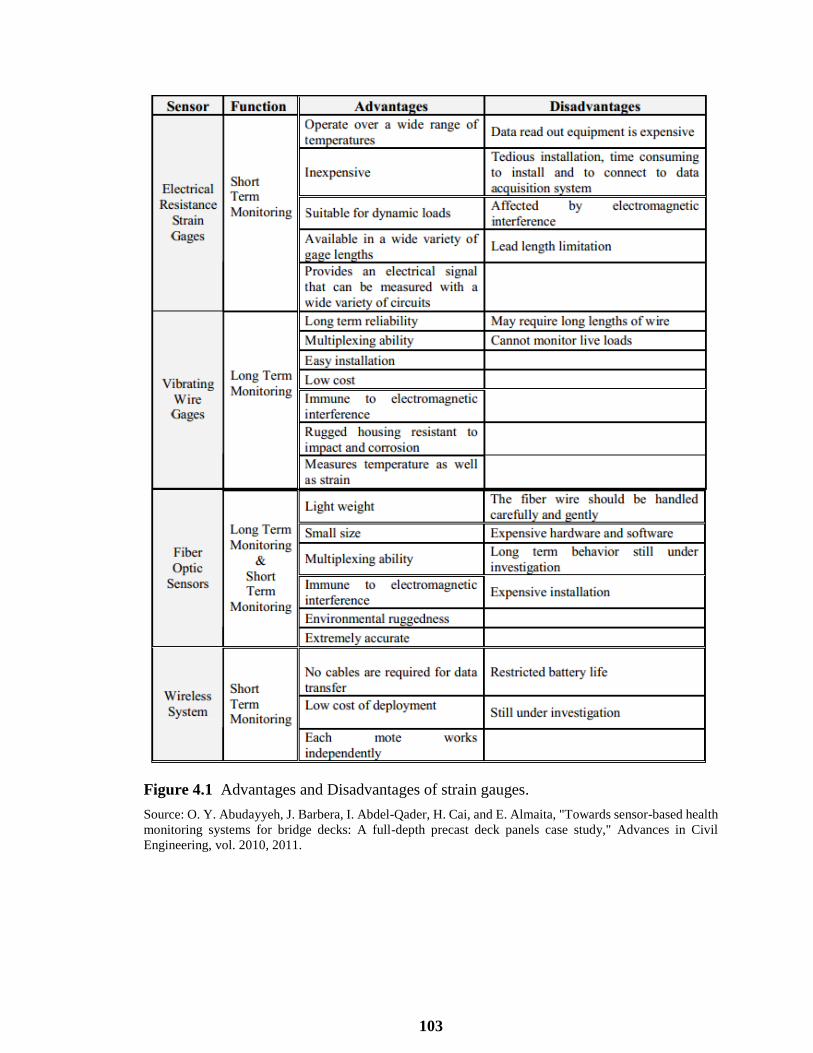
103
Figure 4.1 Advantages and Disadvantages of strain gauges.
Source: O. Y. Abudayyeh, J. Barbera, I. Abdel-Qader, H. Cai, and E. Almaita, "Towards sensor-based health
monitoring systems for bridge decks: A full-depth precast deck panels case study," Advances in Civil
Engineering, vol. 2010, 2011.

104
4.3.6 Displacement Measurement Sensors
Displacement of bridge structures serves as an effective indicator of its structural
performance condition. Large displacements or deformations may create hazardous
conditions for traffic actually on the bridge, and excessive displacements may affect the
bridge’s structural integrity. Displacement monitoring is thus needed. Equipment
measuring the displacement includes linear variable differential transformer, level sensing
station and Global Positioning System (GPS).
The linear variable differential transformer (LVDT) is a commonly used
electromechanical facility for measuring relative displacements based on the principle of
mutual inductance. It consists of a hollow metallic tube and a separate movable
ferromagnetic core. The coils produce an electrical signal that is in proportion to the
position of the moving core. LVDTs are available in a wide range of linear stroke, ranging
from micro-meters to 0.5 meter. The measurement of vertical displacement by the level
sensors is in principle based on the pressure difference. The conventional level sensing
system can detect the elevation difference of about 0.5 mm.
The Global Positioning System (GPS) consists of three parts: the space segment,
the control segment, and the user segment. The space segment is composed of 32 satellites
in six orbital planes. The spacing of satellites in orbits is arranged so that at least six
satellites are within line of sight from any location on the Earth’s surface at all times [30].
The control segment is composed of a master control station, an alternate master control
station, and shared ground antennas and monitor stations. The user segment is composed
of millions of civil, commercial, and scientific users of the standard positioning service.
Basically, a GPS receiver receives the signals sent by the GPS satellites high above the

105
Earth, determines the transit time of each message, computes the distances to each satellite,
and calculates the position of the receiver. Nevertheless, this accuracy is in the order of a
meter and cannot be used for displacement monitoring of bridges. In the practical survey,
the Real Time Kinematic (RTK) technique is used where a reference station provides the
real-time corrections. A RTK system usually consists of a base station receiver and a
number of mobile units. The base station re-broadcasts the phase of the carrier that it
measures, and the mobile units compare their own phase measurements with the ones
received from the base station. This system can achieve a nominal accuracy of 1 cm ± 2
parts-per-million (ppm) horizontally and vertically. Atmospheric conditions affect the
accuracy of GPS measurements.
4.3.7 Accelerometers
Although vibration can be measured in terms of velocity and dynamic displacement as
well, acceleration can be measured more accurately. Accelerometers are widely used to
measure acceleration of structures induced by force or ambient excitations. The
acceleration responses of a bridge are closely related to the serviceability and functionality
of the bridge. Additionally, a vibration testing can be employed to obtain the natural
frequencies, damping ratios, and mode shapes of the global structure, which are directly
associated with the mass, stiffness, and damping characteristics.
Basically an accelerometer is a mass-spring-damper system that produces electrical
signals in proportion to the acceleration of the base where the sensor is mounted. The
following parameters should be considered in selection of accelerometers: usable
frequency response, sensitivity, dynamic range, and thermal transient sensitivity. There are

106
four main types of accelerometers available: piezoelectric type, piezoresistive type,
capacitive type, and servo force balance type.
4.3.8 Weather Stations
In some applications, it is desirable to measure the environmental conditions such as
ambient temperature, humidity, rainfall, air pressure, and solar irradiation. A typical
weather station usually integrates a few types of sensors and can measure the above-
mentioned parameters besides the wind speed and direction. Solar irradiation intensity, air
temperature, and wind are important parameters for deriving the temperature distribution
of structures. With temperature distribution, the thermal effect on the structural responses
can be evaluated quantitatively.
4.3.9 Fiber Optic Sensors
Optical fibers can be used as sensors to measure strain, temperature, pressure, and other
quantities. The sensors modify a fiber so that the quantity to be measured modulates the
intensity, phase, polarization, wavelength of light in the fiber. Accordingly the fiber optic
sensors can be classified into four categories as: intensity modulated sensors,
interferometric sensors, polarimetric sensors, and spectrometric sensors [31].
A significant advantage of the fiber optic sensors is multiplexing, that is, several fiber optic
sensors can be written at the same optical fiber and interrogated at the same time via one
channel. In addition, fiber optic sensors are very small in size and immune to
electromagnetic interferences. They are also suitable for both static and dynamics
measurements with a frequency from hundreds to thousands Hertz. The major drawback
of fiber optic sensors is the high cost of both sensors and the acquisition unit (or readout
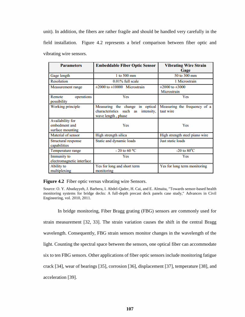
107
unit). In addition, the fibers are rather fragile and should be handled very carefully in the
field installation. Figure 4.2 represents a brief comparison between fiber optic and
vibrating wire sensors.
Figure 4.2 Fiber optic versus vibrating wire Sensors.
Source: O. Y. Abudayyeh, J. Barbera, I. Abdel-Qader, H. Cai, and E. Almaita, "Towards sensor-based health
monitoring systems for bridge decks: A full-depth precast deck panels case study," Advances in Civil
Engineering, vol. 2010, 2011.
In bridge monitoring, Fiber Bragg grating (FBG) sensors are commonly used for
strain measurement [32, 33]. The strain variation causes the shift in the central Bragg
wavelength. Consequently, FBG strain sensors monitor changes in the wavelength of the
light. Counting the spectral space between the sensors, one optical fiber can accommodate
six to ten FBG sensors. Other applications of fiber optic sensors include monitoring fatigue
crack [34], wear of bearings [35], corrosion [36], displacement [37], temperature [38], and
acceleration [39].

108
4.4 Wireless Sensors and Wireless Monitoring
Advances in micro-electro-mechanical systems (MEMS) technology, wireless
communications, and digital electronics have enabled the rapid development of the
wireless sensor technology since the late twentieth century. The wireless sensor is actually
neither one kind of pure sensing technology nor just a new transmission method, but a new
system that can carry out many tasks including SHM. A wireless sensor network can
comprise all of the components in a wire-based SHM system described previously, whereas
it has its unique characteristics as compared with the wire-based SHM systems.
Development of wireless sensors is due to the fact that a robust system may require
a dense network of sensors throughout the system. Traditional sensing systems usually
attempt to develop more accurate sensors of limited quantity at optimized locations. A bio-
system, however, usually comprises a huge number of distributed sensors each with limited
functions. This philosophy inspires researchers to develop a network of low-cost, small
size, large quantity sensors. In addition, the traditional sensing systems are usually wire-
based which have high installation costs. Maintenance of such a monitoring system at a
reliable operating level under the adverse environment for a long period of time is very
difficult. Experience in monitoring civil structures shows that communication wires are
more vulnerable to the environment than sensors themselves [40]. The wireless
transmission provides a more flexible communication manner and sensors can be deployed
and scalable easily.
As a result, Wireless sensor networks have been proposed extensively over the past
several years as a means of alleviating instrumentation costs associated with structural
health monitoring of civil infrastructure. However, low data throughput, unacceptable

109
packet yield rates, and limited system resources have generally plagued many deployments
by limiting the number of sensors and their sampling rate. The sensor networks present
challenges in three broad areas: energy consumption, network configuration and
interaction with the physical world. Therefore, the development of sensor networks
requires technologies from three different research areas: sensing, communication, and
computing (including hardware, software, and algorithms). Structural health monitoring
sensors need to be low-cost, low-power, self-healing, self-organized, and compact.
Researchers at the University of California at Berkeley have developed the open
platform, well known as Berkeley Mote whose ultimate goal is to create a fully autonomous
system within a cubic millimeter volume [41]. Such a system may comprise hundreds or
thousands of sensor nodes each costing as little as about one US dollar. Berkeley Mote was
the first open hardware/software research platform, which allows users to customize
hardware/software for a particular application. The third generation of Mote, the Mica, was
released in 2001. Subsequent improvements to the Mica platform resulted in Mica2,
Mica2Dot, and MicaZ. Another commonly used wireless sensor unit is the Intel Mote
platform Imote [42] and Imote 2 [43].
Berkeley Mote, Intel Mote, and quite a few others have been used for general
purposes in military, environment, health, home, and other commercial areas [44, 45].
These systems have been customized for SHM applications [46-48]. A wireless monitoring
was implemented in the Jindo Bridge, Korea in June 2009, in which 110 wireless nodes
were used. In the structural discipline, researchers from Stanford University have
developed their own wireless sensor unit for SHM [49, 50].

110
4.4.1 Basic Architectures and Features of Wireless Sensors
A wireless sensor node usually consists of four basic components: a sensing unit, a
processing unit, a transceiver unit, and a power unit [44]. The components are carefully
selected to meet the specified functions and keep a total low cost.
The processing unit is a micro-processor (or micro-controller), which controls the
sensing, data processing, computation, and communication with other sensor nodes or the
central station. The on-board processor makes the wireless sensor node intelligent, which
differs from a traditional sensor. The microprocessor has a small storage that stores internal
programs and processed data.
The sensing unit is usually composed of a few sensors and the Analog to Digital
Converter (ADC). The analogue signals collected by the sensors are converted to digital
signals by the ADC, and then sent to the processing unit. It is noted that the ADC in most
general wireless sensor nodes is of only 8 or 10 bits. This is insufficient for vibration
monitoring. In the customized Imote 2 [48], a 16-bits ADC is embedded. The wireless
sensor unit developed in Stanford University [49] has a 16-bits ADC as well.
A transceiver unit connects the node to the network. The transmission distance of
most wireless nodes is about 50 m to 500 m in outdoor environment.
Hence for large civil structures, this transmission range requires the sensor nodes
communicate with the peers and send the data to the base station over the network. The
wireless network has three kinds [51]: star, peer-to-peer, and multi-tier, as shown in Figure
4.3. In the figure, the sensor nodes include generic nodes and gateway nodes. A gateway
node, like the substation in the wired systems, gathers data from the adjacent generic nodes

111
and transmits them to the base station. Most of the smart sensors to date adopt radio
frequency for the wireless communication.
Figure 4.3 Wireless network topology.
The power unit is an important component in wireless sensor node. Currently most
of available smart sensors rely on the battery power supply, which has finite capacity and
finite life. There have been several attempts to harvest energy at sensor nodes locally, for
example, solar cell, wind turbine, mechanical vibration, fuel cells, and mobile supplier.
Solar cell is the current mature technique and was used in wireless monitoring of the Jindo
Bridge [52]. In wireless sensor nodes, communication consumes much more power than
other operations including sensing and processing. Therefore, collected raw data are
processed within the sensing unit to reduce the amount of the raw data transmitted
wirelessly over the network. This also takes advantage of the computational characteristics
of the processor board. Accordingly this distributed computation and monitoring make the
wireless monitoring different from the monitoring using the traditional wired system.
To facilitate this distributed monitoring, the micro-processor has two types of
software: one is the operating system and the other is the engineering algorithms. The
operating system controls the nodes and provides device drivers. One popular operating
system is TinyOS (http://www.tinyos.net), an open-source operating system designed by

112
the University of California at Berkeley. Both Berkeley Mote and Intel Mote run the
TinyOS operating system.
Currently algorithms for distributed monitoring are relatively scarce and simple,
mainly in modal analysis. The complicated monitoring algorithms used in the centralized
monitoring usually need a large amount of memory, heavy computation, and data from
multiple sensors. Consequently transplanting the available monitoring algorithms from the
wired monitoring system directly is not feasible. It is imperative to develop appropriate
algorithms for this distributed monitoring.
4.4.2 Sustainable Operation of the Wireless Sensor Network
Sensors, data acquisition systems, communication and processing units require sustainable
power for truly autonomous operation. Sustainable operation of a sensor network platform
is determined by the correlation of three metrics: (1) Peak energy consumption of the
sensor node components, (2) energy harvesting/generation capability, and (3) rechargeable
battery capacity. If peak sensor energy consumption can eventually drain the battery, the
system is deemed not sustainable. Therefore, designing intelligent hardware and software
protocols is necessary for achieving energy and service equilibrium to enable the on-going
sensing operations. In the following subsections, design decisions for achieving
sustainability are highlighted with respect to these metrics.
Several standards exist for RF communications such as IEEE 802.11 (WLAN),
Bluetooth and IEEE 802.15.4 (ZigBee). Among these standards, ZigBee has become a
popular choice in WSN applications due to its low power requirements and adequate data
rates (up to 250Kbps). For instance, a common chip for ZigBee is Texas Instrument’s
CC2420 2.4 GHz RF transceiver which has been widely used in other smart sensors such

113
as MicaZ and Mica2 [53]. RF chip transmission power output is an important choice for
the overall operation of the WSN. Transmission power determines (i) the communication
distance, (ii) current consumption and (iii) battery output capacity. Therefore, sensor
deployment (i.e. the proximity of the neighboring nodes) for infrastructure structural
system should be done carefully by analyzing the power requirements and sensor node
distances.
RF communication consumes significantly more power than sensor front-end or
microcontroller units. However, distributed computing strategies associated with smart
sensors for health monitoring requires complex computation and processing [54]. Several
new sensor technologies follow this trend such as iMote2 [55] which is based on Intel
XScale processor. On the other hand, FPGAs (Field-Programmable Gate Array) provide
reconfigurable logic, tremendous flexibility and dedicated data-path logic for custom data
processing. This enables previously unattainable computation and control to be realized at
the sensor node. New FPGA technologies target low power sensor applications with ultra-
low power standby and active mode selections [56].
4.4.2.1 Energy Harvesting Among all energy harvesting techniques, solar energy is the
most convenient and suitable for structural health monitoring applications. Photovoltaic
cells provide the highest power concentration (100 mW/cm2)[57]. Structural systems such
as bridges can utilize the ambient solar energy by coupling solar panels with sensor nodes.
Another energy source, although limited in power generation, is piezoelectric material in
which mechanical strains across a material layer generate a surface charge. Several

114
companies such as Microstrain, Inc. produce piezoelectric energy harvesters. These
harvesters can produce up to 30mW at 3.2 VDC with 1.5 g input vibrations.
Solar and piezoelectric energy harvesters can be simultaneously deployed for
redundant and fault-tolerant monitoring operation: The sensors located under direct
sunlight are equipped with two sustainable sources: solar and piezoelectric. The system can
utilize an intelligent controller to switch between available sources (solar or vibration). For
instance, during the daytime when sun irradiation is plentiful, solar provides the main
power not only to power the smart sensors but also to charge up the backup battery. During
the night or cloudy situations, the backup battery and the piezoelectric harvesters can act
as the power source. A multiple-input power electronic converter needs to be implemented
to add the energy of both these sources for energy diversification and increased reliability.
The combination of various energy sources provides adequate power to energize the
sensors and supply the power required for the SoC computation and RF communication.
Other energy harvesting systems, such as mini generators using bridge vibrations
as the power source, or micro wind turbines, have also been considered for health
monitoring applications, however to a much lesser extent than solar power systems.
4.4.2.2 Power Management For sustainability, not only is energy harvesting is critical,
but efficient power management is also necessary. Power management and maintenance of
a reliable operation is ensured by:
Removing the load from energy harvesting source (putting the SoC system into sleep
mode) if power reserves are less than a threshold.
Minimizing the operations requiring high power consumption such as frequent and/or
redundant raw data transmissions.

115
Reserving minimum emergency power for critical instances of sensing such as when
the traffic load is heavy and/or unexpected severe environmental changes occur.
Utilizing ultra-low power components with minimal standby current.
Transmitting only when there is an anomaly or a major change in the structural health
to be reported.
By integrating smart SoC processors, sensor nodes are capable of selfmonitoring their
power generation and power consumption continuously. For continuous use, a power
reserve must be provided in the form of battery to avoid power shortages. Using
rechargeable energy storage such as high capacity (>5000mAh) Li-Ion/Polymer
batteries, the power harvested by photovoltaic cells or piezoelectric energy sources can
extend over a long period of time.

116
4.5 Structural Health Monitoring System of an In-service Highway Bridge
A Structural Health Monitoring System (SMH) using wireless Sensor Networks for an in-
service 6-Span Precast Segmental Box Girder Bridge has been devised (see Section 2.5 for
bridge description), which will be installed and operated by the Public Works Authority -
Qatar (Ashghal, PWA). The deployment of Wireless Sensor Networks in the bridge will
be implemented to evaluate the bridge response and demonstrate the ability of the proposed
long-term monitoring systems to successfully perform on the bridge. The layout of the
sensory system for the bridge is demonstrated in this section. The sensors are in four major
types: accelerometers, temperature sensors, weigh-in-motion sensors, and strain gauges.
4.5.1 Accelerometers
A total of 36 Accelerometers were installed both on the bridge super-and substructures. As
shown in Figure 4.4, one tri-axial accelerometer (A0), nine bi-axial (A2, A3, A5, A7, A9,
A13, A15, A17 and A20), and twenty six uni-axial (A1, A4, A6, A8, A10, A11, A12, A14,
A16, A18, A19, A21, A22 to A35) were installed. The accelerometers are located such that
the longitudinal, lateral, torsional, and vertical motions of the bridge deck and piers can be
measured. Thus, one bi-axial accelerometer will be installed on the south side for
measuring the accelerations in the vertical and lateral directions, while one uni-axial
accelerometer will be installed on the north side to measure the vertical acceleration.
Figure 4.4 Schematic Layout of the Accelerometers.

117
The positions of A1 to A35 are in respectively in the middle and quarter points of
the spans (see Figure 4.4). Except for A0, which will be installed against the end wall at
Abutment 1 to measure the ground motion in the three directions, accelerometers (A1 to
A35) should be mounted on the floor surface inside the box-girder, by brackets bolted into
the concrete, to measure the superstructure vibration at different positions.
4.5.2 Strain Gauges
There are 67 strain gauges which will be installed in the bridge. Sixty four strain meters
will be embedded in the bridge superstructure (see Figure 4.5), and three will be embedded
in pier 3. Sections A1 to A6 are at the middle of each span, sections B1 to B5 are at the end
of spans above the piers. The three strain meters installed in pier 3 are at the same elevation,
measuring vertical strains at the three equally dividend points of the periphery of a circular
cross section to obtain information of the static gravity load on pier 3. The strain meters
are assumed to develop deformations consistent with the concrete, thus measuring the
strain of the concrete at that position.
Figure 4.5 Distribution of strain gauges in the bridge, (a) Sections monitored, (b) A1 to
A6 cross sections, (c) B1 to B5 cross sections.
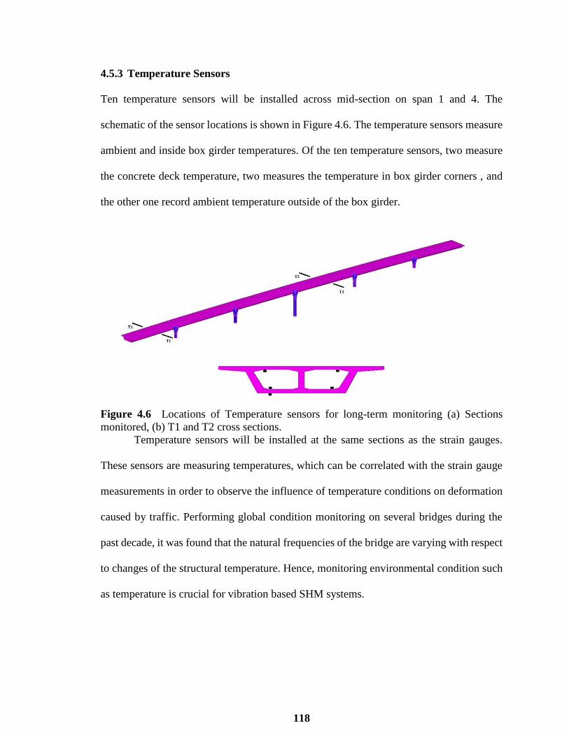
118
4.5.3 Temperature Sensors
Ten temperature sensors will be installed across mid-section on span 1 and 4. The
schematic of the sensor locations is shown in Figure 4.6. The temperature sensors measure
ambient and inside box girder temperatures. Of the ten temperature sensors, two measure
the concrete deck temperature, two measures the temperature in box girder corners , and
the other one record ambient temperature outside of the box girder.
Figure 4.6 Locations of Temperature sensors for long-term monitoring (a) Sections
monitored, (b) T1 and T2 cross sections.
Temperature sensors will be installed at the same sections as the strain gauges.
These sensors are measuring temperatures, which can be correlated with the strain gauge
measurements in order to observe the influence of temperature conditions on deformation
caused by traffic. Performing global condition monitoring on several bridges during the
past decade, it was found that the natural frequencies of the bridge are varying with respect
to changes of the structural temperature. Hence, monitoring environmental condition such
as temperature is crucial for vibration based SHM systems.

119
4.5.4 Weigh-in-motion (WIM) Stations
The traffic loads on the bridge can be monitored by four dynamic WIM stations which
were respectively installed in four lanes of the carriageways (two east-bound and two west-
bound) at the west side approach slab. Each sensor is composed of two bending path pads
and two magnetic loop detectors. The two bending path pads respectively placed on the
left and right hand sides of the lanes were used for vehicle weight detection. The two
magnetic loop detectors respectively installed in the front and rear of the carriageways at a
defined distance were used for measuring axle numbers, axle length, as well as vehicle
speed and height.
4.6 Conclusions
Designing a SHM system is a systematic work integrating various expertise. In this chapter
first the design criteria of SHM for a large-scale bridge is outlined. The commonly used
types of sensory systems is then introduced. As a new and potentially promising sensing,
transmission and monitoring system method, wireless monitoring is specially described in
this chapter. Moreover, design and realization of power harvesting and power usage
optimization for self-sustainable operation of SMH monitoring systems using wireless
sensor networks is briefly discussed.
Finally, the long-term Structural Health Monitoring System using Wireless Sensor
Networks (WSNs) for an in-service highawy bridge is introduced. The results obtained
from the FEA has been utilized to determine sensor locations and measurement types and
could effectively minimize the number of sensors, data for transmission, and volume of
data for processing. Once the hardware of the monitoring system is in place, continuous
monitoring of the structure will be performed. Through continuous monitoring of the

120
dynamic response, vibrational features of the structure can be identified in terms of modal
parameters. Next, damage localization will be performed based on the comparison of
identified modal parameters with the initial values determined for the structure in its perfect
condition. Finite Element Model Updating is then can be performed to update the structural
model to reflect the change in structural dynamic response over time. This will provide the
basis for the future use of the updated model to predict the capacity and remaining life of
the structur

121
CHAPTER 5
OPERATIONAL MODAL ANALYSIS
5.1 Fundamentals of Operational Modal Analysis
The expression Operational Modal Analysis means methods of modal identification which
are based on response measurements only. Early applications of this discipline can be
traced back to the beginning of modal testing in 1960s. The first applications of OMA were
mainly based on the analysis of Power Spectral Density (PSDs) and the identification of
Operational Deflection Shapes (ODSs). An ODS represents the deflection of a structure at
a particular frequency under a generic input and it is usually the result of the contribution
of different modes and ODSs are a close estimate of the actual mode shapes under certain
assumptions. In the 1990s a number of methods working in time domain were developed
and applied in combination with correlation functions, such as Natural Excitation
Techniques (NExT). In the same period the use of ARMA models for modal parameter
estimation started spreading and at the end of the 1990s new effective output-only modal
identification techniques, such as the Frequency Domain Decomposition (FDD) and the
Stochastic Subspace Identification (SSI) became available which could overcome the
limitations of the previous techniques in dealing with closely spaced modes and noise[13].
Nowadays, OMA is a widely accepted tool for modal identification and has been applied
to bridges [58-60], buildings [61, 62], historical structures [63], offshore platforms [64],
wind turbines [65], dams [66], stadia [67]. Applications to ships [68], car bodies [69],
trucks [70], engines [71] and rotating machinery are, instead, directly related to the
mechanical engineering field. In aerospace engineering, examples of output-only tests

122
concern modal identification of aircrafts and shuttles by mean of in-flight tests and studies
about flutter phenomena [72].
OMA techniques are based on the following assumptions:
Linearity: the response of the system to a given combination of inputs is equal to the
same combination of the corresponding outputs;
Stationarity: the dynamic characteristics of the structure do not change over time, which
means, coefficients of differential equations describing the problem are constant with
respect to time;
Observability: test setup must be defined in order to be able to measure the dynamic
characteristics of interest (nodal point must be avoided in order to detect a certain mode
for instance).
As mentioned before, OMA is based on the dynamic response of the structure under
test to noncontrollable and immeasurable loadings such as environmental and operational
loads (traffic, wind, etc.) unlike traditional modal testing. Consequently, some assumptions
about the input are needed. First of all, it is assumed to be a stationary zero mean Gaussian
white noise, which implies that input is characterized by a flat spectrum in the frequency
range of interest and, hence, it gives a broadband excitation, so that all modes are excite
[13]. Since all modes are equally excited, the output spectrum contains full information
about the structure. From a mathematical point of view, signals are completely described
by their correlation functions or by their counterpart in the frequency domain, the auto and
cross power spectra. However, that input actually has a spectral distribution of its own
which is not necessarily flat. Thus, modes are weighted by the spectral distribution of the
input force and the response shows information originating not only from structural modes
but also from the excitation signal. As a result, actual modes must be selected between
information not related to physical modes, such as the ones due to input forces,

123
measurement noise and harmonic vibrations created by rotating parts. Secondly, the
assumption of broadband excitation ensures that all the structural modes in the frequency
range of interest are excited. Assuming that the combined system is excited by a random
input, the second order statistics of the response carry all the physical information about
the system and play a fundamental role in output-only modal identification [13].
5.2 Basic Concepts of Stationary Random Data and Processes
The data observed from a physical phenomenon which can be described by an explicit
mathematical relationship called deterministic. The observed free vibration response of a
Single Degree Of Freedom (SDOF) system under a set of initial conditions is an example
of deterministic data, since it can be defined by an explicit mathematical expression based
on the mass and stiffness properties of the system. On the other hand, random data cannot
be described by explicit mathematical relationships, therefore, the exact value at a certain
time cannot be predicted and they must be described in probabilistic terms.
A random or stochastic process is the combination of all possible physical
understanding of the random phenomenon. A sample function is a single time history
representing the random phenomenon which is one of its physical realizations. A sample
record is a sample function observed over a finite time interval and it can be thought as the
observed result of a single experiment. In the following, focusing the attention in Stationary
Random Processes (SRP) and in particular, Stationary and Ergodic Random Processes
(SERP).
A collection of sample functions which also called ensemble is needed to
characterize a random process. The mean value of the random process can be computed
from the instantaneous values of each function in the ensemble at that time as follows:

124
𝜇𝑥(𝑡)̅ = lim𝐾→∞
1
𝐾∑𝑥𝑘(𝑡̅)
𝐾
𝑘=1
(5.1)
Where 𝑥𝑘(𝑡)̅ is the k-th function in the ensemble, at a certain time instant 𝑡̅.
Similarly, the autocorrelation function can be computed by taking the ensemble
average of the product of instantaneous values at time instants 𝑡̅ and 𝑡̅ + 𝜏:
𝑅𝑥𝑥(𝑡̅, 𝑡̅ + 𝜏) = lim𝐾→∞
1
𝐾∑𝑥𝑘(𝑡̅)𝑥𝑘(𝑡̅ + 𝜏)
𝐾
𝑘=1
(5.2)
Whenever the quantities expressed by Equations (5.1) and (5.2) do not change when
the considered time instant t varies, the random process is said to be stationary. The mean
value is independent of the time t and the autocorrelation depends only on the time lag τ
for stationary random processes,
𝜇𝑥(𝑡̅) = 𝜇𝑥 (5.3)
𝑅𝑥𝑥(𝑡,̅ 𝑡̅ + 𝜏) = 𝑅𝑥𝑥(𝜏) (5.4)

125
In the following sections the basic properties for stationary random records such as
probability density functions, auto- and cross-correlation functions, autoand cross-spectral
density functions are briefly discussed. In fact, the above-mentioned properties are primary
tools of signal analysis and commonly used to prepare the data for most OMA techniques.
5.2.1 Spectral Density Functions
Power spectral density function (PSD) is a statistical function which shows the strength of
the variations (energy) as a function of frequency. In other words, it shows at which
frequencies variations are strong and at which frequencies variations are weak. The unit of
PSD is energy per frequency(width) and energy can be obtain within a specific frequency
range by integrating PSD within that frequency range. Computation of PSD is done directly
by the method called Fast Fourier Transform (FFT) or computing autocorrelation function
and then transforming it which will be briefly described. PSD is a useful tool for identifying
oscillatory signals in time series data and their amplitude.
Considering a sample record 𝑥𝑘(𝑡) of finite duration T from stationary random
processes. Its Fourier transforms exist as a consequence of the finite duration of the signals
and can be written as follows:
𝑋𝑘(𝑓, 𝑇) = ∫ 𝑥𝑘(𝑡)𝑒−𝑖2𝜋𝑓𝑡𝑑𝑡
𝑇
0
(5.5)
and the two-sided auto- and cross-spectral density functions are defined as follows:

126
𝑆𝑥𝑥(𝑓) = lim𝑇→∞
𝐸 [1
𝑇𝑋𝑘∗(𝑓, 𝑇)𝑋𝑘(𝑓, 𝑇)] (5.6)
where * represents complex conjugate. Two-sided means that 𝑆(𝑓) is defined for f in the
range (-∞, +∞) and the expected value operation is working over the ensemble index k.
The one-sided auto- and cross-spectral density functions, with f varying in the range (0,
+∞), are given by:
𝐺𝑥𝑥(𝑓) = 2𝑆𝑥𝑥(𝑓) = 2 lim𝑇→∞
𝐸[|𝑋𝑘(𝑓, 𝑇)|2] 0 ˂ 𝑓 ˂ + ∞ (5.7)
The two-sided spectral density functions are more commonly utilized in theoretical
derivations and mathematical calculations, whereas the one-sided spectral density
functions are typically used in the applications. In practical applications the one-sided
spectral density functions are always the result of Fourier transforms of records of finite
length (T < ∞), along with averaging of a finite number of ensemble elements.
Before analyzing the computation of PSDs in practice, it is worth noting that PSDs
and correlation functions are Fourier transform pairs. Accordingly, the two-sided spectral
density functions are the Fourier transforms of the correlation functions:

127
𝑆𝑥𝑥(𝑓) = ∫ 𝑅𝑥𝑥(𝜏)𝑒−𝑖2𝜋𝑓𝜏𝑑𝜏
+∞
−∞
(5.8)
Equation (5.8) is also called the Wiener-Khinchin relation. The auto-spectral
density functions are real-valued functions, on the other hand, the cross-spectral density
functions are complex-valued. In terms of one-sided spectral density functions, the
correspondence with the correlation functions is given by:
𝐺𝑥𝑥(𝑓) = 4∫ 𝑅𝑥𝑥(𝜏) cos(2𝜋𝑓𝜏) 𝑑𝜏∞
0
(5.9)
It is worth pointing out two important properties of Gaussian random processes for
practical applications. First, it can be shown that if a Gaussian process undergoes a linear
transformation, the output is still a Gaussian process [73]. Furthermore, assuming a sample
record of an ergodic Gaussian random process with zero mean, it can be proven that the
Gaussian probability density function is completely determined by the knowledge of the
auto-spectral density function [73].
In fact, considering that:

128
𝜎𝑥2 = ∫ 𝑥2𝑝(𝑥)𝑑𝑥
+∞
−∞
≈ ∫ 𝐺𝑥𝑥(𝑓)𝑑𝑓∞
0
(5.10)
𝐺𝑥𝑥(𝑓) alone determines 𝜎𝑥 [73]. Hence, spectral density functions and their
Fourier transform pairs (the correlation functions) play a fundamental role in the analysis
of random data.
In practical applications, PSDs can be obtained by computing the correlation
functions first and then Fourier transforming them. This approach is known as the
Blackman-Tukey procedure [13]. Another approach, known as the Welch procedure, is,
instead, based on the direct computation of the FFT of the records and the estimation of
the PSDs in agreement with Equation (5.7). The Welch procedure is less computational
demanding than the Blackman-Tukey method, but it requires some operations on the signal
in order to improve the quality of the estimates.
Additionally, based on Equation (5.7), the one-sided auto-spectral density function
can be estimated by dividing a record into 𝑛𝑑 contiguous segments, each of length T=NΔt,
Fourier transforming each segment and then computing the auto-spectral density through
an ensemble averaging operation over the 𝑛𝑑 subsets of data [13].
Even if the direct computation via FFT of the spectral density function is
advantageous from a computational point of view, specific strategies are required to
eliminate the errors originating from the fact that the estimates are based on records of
finite length. A sample record x(t) can be interpreted as an unlimited record v(t) multiplied
by a rectangular time window u(t):

129
𝑥(𝑡) = 𝑢(𝑡) 𝑣(𝑡) 𝑢(𝑡) = {1 0 ≤ 𝑡 ≤ 𝑇0 𝑒𝑙𝑠𝑒𝑤ℎ𝑒𝑟
(5.11)
Therefore, the Fourier transform of x(t) is given by the convolution of the Fourier
transforms of u(t) and v(t). The Fourier transformof a rectangular signal is basically a sinc
function (Figure 5.1) with side lobes characterized by a fairly large amplitude with respect
to the main lobe (the amplitude difference is just _13 dB).
Figure 5.1 Discrete Fourier Transform (DFT) of a rectangular window: amplitude.
The large side lobes of |U(f)| allow the energy at a certain frequency to spread to
nearby frequencies, causing large amplitude errors. This phenomenon is also known as
leakage and it may introduce significant distortions in the estimated spectra, in particular
in the presence of data characterized by narrow bandwidth. Nevertheless, it does not
happen when the analyzed data are periodic with a period equal to the record length. In
such a case, in fact, the discrete frequency values, equally spaced at Δf=1/T, coincide with
zeros of the spectral window in the frequency domain with the only exception of the

130
frequency line in the main lobe. The result is an exact reproduction of the correct spectrum.
Thus, in order to suppress the leakage problem, data are made periodic by tapering them
by an appropriate time window, which eliminates the discontinuities at the beginning and
end of the analyzed record. There are different options for the choice of the window [74].
Here, the most commonly employed window is introduced. It is the full cosine tapering
window, also known as Hanning window, which is given by:
𝑢𝐻𝑎𝑛𝑛𝑖𝑛𝑔(𝑡) = {1 − cos2(𝜋𝑡
𝑇) 0 ≤ 𝑡 ≤ 𝑇
0 𝑒𝑙𝑠𝑒𝑤ℎ𝑒𝑟 (5.12)
The highest side lobe level of the Hanning window is 32 dB below the main lobe.
Thus, leakage is minimized. The use of the Hanning window to compute spectral density
estimates by Fourier transform techniques implies a loss factor of 3/8. As a consequence,
a rescaling is needed to obtain spectral density estimates characterized by the correct
magnitude.
5.2.2 Fundamentals of Matrix Algebra
Most OMA methods are based on fitting of an assumed mathematical model to the
measured data. In such a case, the ultimate goal is to determine the unknown modal
parameters of the system from the measured response of the structure under certain
assumptions about the input. This is an example of inverse problem. The solution of inverse
problems is based on matrix algebra, including methods for matrix decomposition.

131
Additionally, Matrix algebra plays an important role in the case of those OMA
methods that extract the modal parameters without assumptions about the system that
produced the measured data. Thus, a review of basics of matrix algebra and of some
methods for the solution of inverse problems is presented to understand the mathematical
background of the OMA methods described in consequent sections.
Consider the generic matrix:
[𝐴] = [
𝑎1,1 ⋯ 𝑎1,𝑀⋯ 𝑎𝑖,𝑗 …𝑎𝐿,1 … 𝑎𝐿,𝑀
] (5.13)
of dimensions L×M. Its generic element is 𝑎𝑖,𝑗, where the index i=1, . . ., L indicates the
row number and the index j=1, . . ., M refers to the column number. The matrix [A] can be
real-valued or complex valued, depending if its elements are real or complex numbers.
When the matrix [A] presents a linear operator transforming a certain vector {𝑥}
into a new vector {𝑦}:
{𝑦} = [𝐴]{𝑥} (5.14)

132
When the vector {𝑦} in Equation (5.14) can be computed via the matrix
multiplication [A]{𝑥}, and via the scalar product λ{𝑥}, λ is defined an eigenvalue of [A]
and {𝑥} is the corresponding eigenvector. The eigenvalues are obtained as a solution of the
characteristic equation:
𝑑𝑒𝑡([𝐴] − 𝜆[𝐼]) = 0 (5.15)
and the corresponding eigenvectors are determined by replacing the obtained eigenvalues
𝜆𝑘[𝐼] into Equation (5.16):
([𝐴] − 𝜆𝑘[𝐼]){𝑥𝑘} = {0} (5.16)
If the matrix [A] is Hermitian or symmetric, the eigenvectors corresponding to
distinct eigenvalues are orthogonal (their dot product is zero) and its eigenvalues are real.
If the symmetric matrix [A] is positive-definite the eigenvalues are real and positive and
the matrix [A] is invertible.
The matrix inversion can be implemented more effectively when dealing with
systems of equations by decomposing the matrix into factors. There are different types of

133
matrix decomposition methods. The eigenvalue decomposition (EVD) provides an
expression for the invertible square matrix [A] as a product of three matrices:
[𝐴] = [𝑈][Σ][𝑉]𝑇 (5.17)
where [Σ] of dimensions L×M is a rectangular diagonal matrix containing the singular
values which arranged in descending order. The first r singular values are positive, while
the remaining singular values 𝜎𝑟+1, . . ., 𝜎𝑀 are all equal to zero. [U] and [V] are orthogonal
matrices of dimensions L×L and M×M, respectively. The column vectors {𝑢1}, . . ., {𝑢𝑟} of
[U] span the range of [A], while the vectors {𝑣𝑟+1}, . . ., {𝑣𝑀} span the null space of [A].
If [A] is a complex-valued matrix, the Singular Value Decomposition (SVD) is generalized
by replacing the transpose with the Hermitian operator.
The SVD has many applications in signal processing and for the solution of inverse
problems, including the computation of pseudo-inverse, least squares fitting of data, matrix
approximation and rank determination. In the common case in which [A] is a square, real-
valued matrix, [Σ] can be explained as a scaling matrix, while [U] and [V]T can be regarded
as rotation matrices. Hence, the SVD can be interpreted as a series of three geometrical
transformations, namely a rotation, a scaling, and another rotation [13]. The SVD is also
used for the computation of the Moore-Penrose pseudoinverse of a matrix.
Other decomposition methods such as LQ decomposition and RQ decomposition
for square matrices result in the conversion of the matrix [A] into a product of an orthogonal

134
matrix [Q] and an upper [R] or lower [L] triangular matrix. The Cholesky factorization,
instead, is a decomposition of a real-valued, symmetric, and positivedefinite matrix into
the product of a lower triangular matrix and its transpose. Further details about matrix
algebra and decompositions can be found elsewhere [75].
5.2.3 Inverse Problems
A common approach in OMA is the fitting of a hypothesized model to the measurements
in order to obtain the unknown modal parameters. The approach to fitting depends on the
selected model. For explaining the fundaments, in this section the main concepts are
demonstrated with reference to a simple and general polynomial function:
𝑦(𝑥) = 𝑐0 + 𝑐1𝑥 + 𝑐2𝑥2 +⋯+ 𝑐𝐿−1𝑥
𝐿−1 (5.18)
No specific references are made to the theoretical background of OMA at this stage,
but the application of these concepts in different contexts is straightforward and it will
become more clear when the theory of some OMA methods is reviewed in the subsequent
sections.
Assuming that M measurements have been carried out, the L unknown model
parameters (𝑐0,𝑐1, . . .,𝑐𝐿−1) can be determined from the following set of M equations which
are rearranged in matrix form as:

135
{𝑦} = {
𝑦1…𝑦𝑖…𝑦𝑀
} =
[ 1 𝑥1 𝑥1
2 ⋯ 𝑥1𝐿−1
⋯ ⋯ ⋯ ⋯ ⋯
1⋯1
𝑥𝑖⋯𝑥𝑀
𝑥𝑖2
⋯𝑥𝑀2
⋯⋯⋯
𝑥𝑖𝐿−1
⋯𝑥𝑀𝐿−1]
{
𝑐0⋯𝑐𝑖⋯𝑐𝐿−1}
= [𝑀]{𝑐} (5.19)
Considering that the setting of the problem in matrix form does not need a linear
functional relation between y and x. A linear combination of basis functions of x is also
suitable. Typically, there are more measurements than unknowns (M>L), so that an
overdetermined set of equations can be defined and measurements are noisy. It is worth
mentioning that when the number of unknowns L exceeds the number of equations M, the
problem is definitely underdetermined. Thus, the inverse problem cannot lead to a unique
solution and additional information has to be provided or the number of unknowns has to
be reduced. On the other hand, when M>L the problem can not only be overdetermined,
but also be evendetermined or underdetermined, depending on the eventual presence of
analogous measurements which do not provide additional information. Therefore, the rank
of the matrix in Equation (5.19) actually determines if the problem is overdetermined or
underdetermined. But in practical applications, the sole determination of the rank of a
matrix can be misleading due to the presence of measurement noise.
In similar conditions the SVD of the matrix can provide more valuable information
about the type of inverse problem. As a matter of fact, the condition number κ which is the
ratio between the maximum and minimum absolute values of singular values, can be
computed to evaluate whether the matrix is noninvertible (𝐾 = ∞), ill-conditioned (K very
large) or invertible (small K). In ill-conditioned problems the small singular values magnify

136
the errors, so considering only the subset of the largest singular values can reduce their
effect. The selection of the number of singular values to be maintain is usually depends on
sorting of the singular values and identification of jumps [13].
Assuming that a curve fitting the measured data has been found and the functional
relation between y and x in Equation (5.18) has been established, there will be an error (or
residual) corresponding to the i-th measurement. It can be computed as difference between
the predicted (𝑦𝑖,𝑝𝑟𝑒𝑑) and the measured (𝑦𝑖,𝑚𝑒𝑎𝑠) value of y:
휀𝑖 = 𝑦𝑖,𝑝𝑟𝑒𝑑 − 𝑦𝑖,𝑚𝑒𝑎𝑠 (5.20)
Therefore, the objective of the analysis is the estimation of the unknown
coefficients (𝑐0,𝑐1, . . .,𝑐𝐿−1) from the measured data in a way able to minimize the sum of
the residuals when all measurements are considered.
Different definitions for the residuals can be selected, considering that the selected
error definition has an influence on the estimation of the unknown parameters. For instance,
when the data are characterized by the presence of very large and very small values in the
same set, the computation of the residuals according to Equation (5.20) skew the inversion
towards the largest values. Hence, one of the following definitions of residual can be
considered as an alternative:

137
휀𝑖 =𝑦𝑖,𝑝𝑟𝑒𝑑 − 𝑦𝑖,𝑚𝑒𝑎𝑠
𝑦𝑖,𝑝𝑟𝑒𝑑 (𝑝𝑟𝑜𝑝𝑜𝑟𝑡𝑖𝑜𝑛𝑎𝑙 𝑒𝑟𝑟𝑜𝑟) (5.21)
휀𝑖 = log(𝑦𝑖,𝑚𝑒𝑎𝑠) − log(𝑦𝑖,𝑝𝑟𝑒𝑑) (log 𝑑𝑖𝑓𝑓𝑒𝑟𝑒𝑛𝑐𝑒) (5.22)
Additional error definitions can be found in the literature [76].
A global evaluation of the quality of the fit can be obtained from the computation
of the norm of the vector of residuals {휀}:
{휀} =
{
휀1⋯휀𝑖⋯휀𝑀}
(5.23)
The generic n-norm is given by:
𝐿𝑛 = √∑|휀𝑖|𝑛
𝑖
𝑛 (5.24)

138
The order of the norm is related to the weight placed on the larger errors, in other
words the higher the order of the norm, the higher the weight of the larger errors. Three
notable norms are:
𝐿1 =∑|휀𝑖|
𝑖
(5.25)
𝐿2 = √∑|휀𝑖|2
𝑖
= √{휀}𝑇{휀} (5.26)
𝐿∞ = max (|휀1|, … , |휀𝑖|, … , |휀𝑀|) (5.27)
The 𝐿1 norm provides a powerful solution, since it is not sensitive to a few large
errors in the data. The 𝐿2 norm is compatible with additive Gaussian noise present in the
data and the 𝐿∞ norm considers only the largest error and is the most sensitive to errors in
the data.
Based on the previous definitions, the least squares solution of the inverse problem
can be defined as the set of values of the coefficients (𝑐0,𝑐1, . . .,𝑐𝐿−1) that minimizes the
𝐿2 norm of the vector of residuals. Therefore, setting the derivative of this 𝐿2 norm with
respect to {𝑐} equal to zero, under the assumption that [𝑀]𝑇[𝑀] is invertible the least
squares solution provides the following estimate of the model parameters:

139
{𝑐} = ([𝑀]𝑇[𝑀])−1[𝑀]𝑇{𝑦𝑚𝑒𝑎𝑠} = [𝑀]+{𝑦𝑚𝑒𝑎𝑠} (5.28)
The least squares method is a standard approach to the approximate solution of
overdetermined systems. It works well when the uncertainties affect the dependent
variable. If substantial uncertainties affect also the independent variable, the total least
square approach has to be adopted. This method is able to consider the observational errors
on both dependent and independent variables. More mathematical details of the method
can be find in the literature [75].
5.3 Classification of OMA Techniques
A classical distinction between Modal identification methods is based on the domain of
implementation. OMA methods directly based on time histories of the output signals are
referred to as time domain methods. Methods based on spectral density functions and
Fourier transform of signals are, instead, referred to as frequency domain methods. Even
if this distinction may look artificial, since they simply consider different representations
of the same signal and it is always possible to transform signals from one domain to the
other, there are some differences in terms of practical applications. In fact, time domain
methods are usually better conditioned than the frequency domain counterpart. This is
mainly related to the effect of the powers of frequencies in frequency domain equations.
Moreover, time domain methods are usually more suitable for handling noisy data, and
they avoid most signal processing errors such as leakage if applied directly to raw time
domain data. On the other hand, in noisy measurement conditions, averaging is easier and
more efficient in frequency domain.

140
Another distinction is between Single Degree Of Freedom (SDOF) and Multiple
Degree Of Freedom (MDOF) methods based on the assumption about the number of modes
determining the structural response. When in a certain frequency band only one mode is
assumed to be important and the structural response in that frequency range depends only
on that mode, the parameters of this mode can be determined separately, leading to the
SDOF methods. Even if these methods are very fast and characterized by a low
computational burden, the SDOF assumption is a reasonable approximation only if the
modes of the system are well decoupled. On the other hand, MDOF methods are necessary
when dealing with close coupled modes or even coincident modes to properly identify the
different modes contributing to the overall structural response.
5.4 Operational Modal Analysis in the Frequency Domain
5.4.1 The Basic Frequency Domain (Peak-Picking) Method
The most undemanding method for modal parameter estimation from output-only data is
the Basic Frequency Domain (BFD) method [77], also called the Peak-Picking method. In
the past, it has been widely used for identification purposes in civil engineering and a
practical implementation was made by Felber [78]. The name of the method is related to
the fact that natural frequencies are determined as the peaks of the Power Spectral Density
(PSD) plots, obtained by converting the measured data to the frequency domain by the
Discrete Fourier Transform (DFT).
The BFD technique is a SDOF method for OMA. In fact, it is based on the
assumption that, around a resonance, only one mode is dominant. When it happens, taking

141
into account the following expression for the Frequency Response Function (FRF) and that
the input spectrum is assumed to be constant.
[𝐻(𝜔)] =∑[[𝐴]𝑟
𝑗𝜔 − λ𝑟+
[𝐴]𝑟∗
𝑗𝜔 − λ𝑟∗]
𝑁
𝑟=1
(5.29)
being [𝐴]𝑟 the residue matrix, N the number of modes and λ𝑟 the r-th eigenvalue. The
output spectrum matrix, which can be expressed as follows:
[𝐺𝑦𝑦(𝜔)] = ∑∑[[𝑅𝑘]
𝑗𝜔 − λ𝑟+
[𝑅𝑘∗]
𝑗𝜔 − λ𝑟∗]
𝑁
𝑟=1
𝑁
𝑘=1
[𝐶] [[𝑅𝑠]
𝑗𝜔 − λ𝑠+
[𝑅𝑠∗]
𝑗𝜔 − λ𝑠∗]
𝐻
(5.30)
can be approximated by considering only the contribution of the dominant mode, for
example the r-th mode, as:
[𝐺𝑦𝑦(𝜔)] ≈[𝑅𝑟]
𝑗𝜔 − λ𝑟+
[𝑅𝑟∗]
𝑗𝜔 − λ𝑟∗ (5.31)

142
where the residues are related to the mode shape.
It is clear that in this case the power spectral density (PSD) matrix is of rank one.
Therefore, at resonance any column of the PSD matrix can be considered as an estimate of
the corresponding mode shape, up to a scaling factor being the input unmeasured.
From a practical point of view, first to identify the peaks corresponding to structural
resonances, the trace of the PSD matrix (the sum of the autospectra) at each discrete
frequency value is computed. Then, the mode shapes associated to the identified
frequencies are obtained from one of the columns of the PSD matrix. A reference sensor
for the computation of the cross-spectral densities with all other measurement channels has
to be selected considering that reference sensor cannot be a sensor placed at a node of the
mode shape. Depending on the geometry of the structure and the adopted sensor layout, a
single reference sensor could be insufficient to identify all the modes and at least a couple
of reference sensors with different orientation have to be adopted.
Additionally, Identification of actual natural frequencies can be carried out by
looking not only at peaks of the spectra but also by inspecting the coherence function
between two channels, defined as:
𝛾𝑟𝑠2 (𝑓) =
|𝐺𝑟𝑠 (𝑓)|2
𝐺𝑟𝑟 (𝑓)𝐺𝑠𝑠 (𝑓) (5.32)

143
and assuming values between 0 and 1; 𝐺𝑟𝑠 (𝑓) is the value of the crosss-pectrum between
channels r and s at the frequency f, while 𝐺𝑟𝑟 (𝑓) and 𝐺𝑠𝑠 (𝑓) are the values of the auto-
spectra of channel r and channel s, respectively, at the same frequency.
If (f) is a resonant frequency, the coherence function is close to one because of the
high signal-to-noise ratio at that frequency. This characteristic is helpful in the
discrimination between real eigenfrequencies and peaks due to disturbances. Also, the
coherence function can be useful for the identification of the nature of a mode. With the
combination of information from spectra and coherence functions even it is possible to
identify closely spaced modes. However, the success of the identification process heavily
depends on the geometry of the structure and the skill of the analyst. Also, when the peaks
in the spectra are not clear for instance in the case of noisy measurements, the results of
modal identification suffer a certain degree of subjectivity.
The BFD method allows the evaluation of the modal properties and the accuracy of
the estimated eigenfrequencies depends on the frequency resolution of the spectra. In other
words, to obtain good natural frequency estimates, a fine frequency resolution is necessary.
In order to estimate damping ratios from the spectra, it is suggested to use the half-power
bandwidth method [77]. However, a number of studies have shown that they are not
accurate [79, 80].
In summary, this method is very simple and not demanding from computational
point of view which makes it a useful analysis tool for the analyst, especially during field
tests, to get a quick insight about effectiveness of measurements and results of dynamic
identification [13]. However, it suffers some drawbacks due to the SDOF assumption. The
BFD technique works well when damping is low and modes are well-separated, but if these

144
conditions are violated it may lead to inaccurate results. In fact, the method, instead of the
actual mode shapes, identifies the Operational Deflection Shapes (ODSs) which are a
combination of all mode shapes. They are a good approximation of actual mode shapes
only if one mode is dominant at the considered frequency. In case of closely-spaced modes,
ODS is the superposition of multiple modes. Another important drawback is that the
selection of eigenfrequencies can become a subjective task if the spectrum peaks are not
very clear. Moreover, eigenfrequencies are estimated on a local basis by looking at single
spectra and a fine frequency resolution is required in order to obtain a good estimation of
the natural frequency.
5.4.2 The (Enhanced) Frequency Domain Decomposition
The main drawbacks of the BFD method have been overcome by the introduction of the
Frequency Domain Decomposition (FDD) technique [69]. This method was originally
applied to FRFs and was known as Complex Mode Indicator Function (CMIF) in order to
point out its ability to detect multiple roots and possibility count the number of dominant
modes at a certain frequency [81]. The method has been then better systematized by
Brincker and applied to response spectrum data.
A theoretical verification of the method is based on the modal expansion of the
structural response:
{𝑦(𝑡) = [Φ]{𝑝(𝑡)}} (5.33)

145
where [Φ] is the modal matrix and {𝑝(𝑡)} the vector of modal coordinates. From Equation
(5.33), the correlation matrix of the responses can be computed:
𝑅𝑦𝑦(𝜏) = 𝐸 [{𝑦(𝑡 + 𝜏)}{𝑦(𝑡)}𝑇] = [Φ][𝑅𝑝𝑝(𝜏)][Φ]𝑇 (5.34)
The PSD matrix can be obtained from Equation (5.34) by taking the Fourier
transform:
[𝐺𝑦𝑦(𝜔)] = [Φ][𝐺𝑝𝑝(𝜔)][Φ]𝐻 (5.35)
Taking into account that the Singular Value Decomposition (SVD) of the PSD
matrix at a certain frequency ω the following factorization can be derived:
[𝐺𝑦𝑦(𝜔)] = [U][Σ][V]𝐻 (5.36)
where [U] and [V] are the unitary matrices holding the left and right singular vectors and
[Σ] is the matrix of singular values which should be arranged in descending order. Since

146
the PSD is a Hermitian and positive definite matrix, [U] = [V] and the decomposition of
Equation (5.36) can be rewritten as:
[𝐺𝑦𝑦(𝜔)] = [U][Σ][U]𝐻 (5.37)
The comparison between Equations (5.35) and (5.37) demonstrate that it is possible
to identify a one-to-one relationship between singular vectors and mode shapes;
furthermore, the singular values are related to the modal responses which can be used to
define the spectra of equivalent SDOF systems characterized by the same modal
parameters as the modes contributing to the response of the MDOF system under
investigation. As mentioned before, the SVD provides the singular values arranged in
descending order, so near a resonance the first singular value contains the information
about the dominant mode at that frequency. Moreover, since the number of nonzero
elements in [Σ] is the rank of the PSD matrix at the considered frequency, this feature is
used to identify closely spaced or even coincident modes. In other words, the number of
dominant singular values (the rank of the output PSD matrix) at a certain frequency the
number of modes that give a significant contribution to the structural response at that
particular frequency are equivalent.
Assuming at the frequency ω, only one mode is dominant and also the selected
frequency is associated to the peak of resonance of the k-th mode, the PSD matrix

147
approximates to a rank one matrix and there will be only one term on the right side of
Eequation (5.37):
[𝐺𝑦𝑦(𝜔)] = 𝜎1{𝑢1}{𝑢1}𝐻 𝜔 → 𝜔𝑘 (5.38)
In such a case, the first singular vector {𝑢1} is an estimate of the mode shape of the
k-th mode:
{�̂�𝑘} = {𝑢1(𝜔𝑘)} (5.39)
and the corresponding singular value 𝜎1 belongs to the auto power spectral density function
of the corresponding SDOF system. In case of repeated modes, the PSD matrix rank is
equal to the number of multiplicity of the modes.
By comparing the mode shape estimate {�̂�𝑘} at the peak with the singular vectors
associated to the frequency lines around the peak, the singular values whose singular
vectors show a correlation with {�̂�𝑘} higher than a user-defined threshold can be identified,
which called MAC Rejection Level. Such singular values define the equivalent SDOF PSD
function. The Modal Assurance Criterion (MAC) is used as a measure of the correlation
between two modal vectors [82]. This equivalent SDOF PSD function is used, when

148
applying the Enhanced Frequency Domain Decomposition (EFDD) algorithm [83, 84], to
estimate the modal damping ratio and obtain an estimate of the natural frequency which is
independent of the frequency resolution of the spectra computed by the Fast Fourier
Transform (FFT) algorithm. In fact, an approximated correlation function of the equivalent
SDOF system can be obtained by the inverse Fourier transform of the equivalent SDOF
PSD function. From the free decay function of the SDOF system, the damping ratio can be
calculated by the logarithmic decrement technique. A similar procedure is adopted in order
to extract natural frequencies, carrying out a linear regression on the zero crossing times of
the equivalent SDOF system correlation function and taking into account the relation of
damped an un-damped natural frequency [13].
The FDD method allows to overcome the typical drawbacks of the BFD technique
such as identification of closely spaced modes. However, it worth to mention that in this
case the mode shape estimates could be biased. The singular vectors are forced to be
orthogonal by the SVD, if the experimental mode shapes are also orthogonal the obtained
estimates are unbiased. However, this is not always true; in such a case, estimation of the
mode shape for the closely spaced modes are biased and the bias mainly affects the weak
mode, while the mode shape estimate for the dominant mode is still good. The larger the
difference between the first and second singular value, the smaller the error due to the bias.
Hence, the mode shape estimates should be obtained from singular vectors at frequencies
characterized by the largest difference between the first and second singular value. This
frequency might be different from the frequency of the peak in the presence of closely
spaced modes.

149
The method described above is the classical implementation of the FDD/EFDD
method, however, alternate methods are possible to find in the literature [85, 86]. In
particular, an alternative implementation of FDD based on EVD instead of SVD is also
available [87]. It is worth mentioning the so-called Frequency-Spatial Domain
Decomposition (FSDD) [62] as another variants of the FDD method, where spatial filtering
has been applied to enhance the estimation of modal frequencies and damping ratios. The
FSDD makes use of the mode shapes estimates computed via SVD of the output PSD
matrix to enhance PSDs. The use of the estimated mode shapes as weighting vectors gives,
results in an enhanced PSD which can be approximated as a SDOF system therefore, a
SDOF curve fitter may be used to estimate the natural frequency and the damping ratio of
the considered mode.
5.5 Spectral Kurtosis Estimation of Harmonic Excitations
5.5.1 Theoretical Background
The Spectral Kurtosis Estimator (SK) is a higher order unbiased statistical estimator
associated with an accumulated Power Spectral Density (PSD) estimate, it is given by [88]:
2
2
1
11 ,
1
MSMSK
M S
(5.40)

150
where 𝑆1(𝑓𝑘) = ∑ 𝑃𝑖𝑀𝑖=1 (𝑓𝑘) represents the sum at each frequency bin, 𝑓𝑘, 𝑖 = 0, 𝑁/2 , of
M consecutive FFT raw power estimates, and 𝑆2(𝑓𝑘) = ∑ 𝑃𝑖2(𝑓𝑘)
𝑀𝑖=1 the sum of their
squares. It is worth mentioning that in the case of a pure Gaussian time domain signal,
statistical expectation of the SK estimator is unity at each frequency bin, although the
power spectrum may have an arbitrary spectral shape.
In order to quantify the expected statistical fluctuations of the SK estimator around
its unity mean, the exact analytical expressions of the infinite series of the statistical
moments of the SK estimator can be obtained [88]. Its first four centralized standard
moments in terms of the accumulation length 𝑀 as follows:
(5.41)
where Γ(𝑧) = ∫ 𝑡𝑧−1∞
0𝑒−𝑡𝑑𝑡 is the Euler’s gamma function.
However, the variance μ2≡ 𝜎2 of the SK estimator in Equation (5.41) is not
sufficient for assigning standard symmetric deviations about the mean. A series expansion
of μ3 shows that the probability density function (PDF) of the SK estimator has a skewness
that does not vanish faster than 10/√𝑀. Hence, the asymmetry of the PDF distribution
around its mean must be taken into consideration, for small accumulation lengths M, in

151
order to estimate the true asymmetric statistical fluctuations of the SK estimator about its
mean[88].
For 𝑀 ≥ 24, accurate detection thresholds of non-Gaussian spectral components
corresponding to a preferred probability of false alarm (PFA) can be computed by
providing a 4-moment Pearson Type IV approximation of the SK probability density
function (PDF). This approach can be generalized and used for 6 ≤ 𝑀 ≤ 23 by either
deriving a 3-moment Pearson Type IV approximation or a more computationally
convenient Pearson Type III (gamma distribution) approximation which can provide
accurately enough PFA thresholds for most practical applications [88].
The Pearson Type III approximation of the SK cummulative probability
distribution function (CF), assuming the shortcut notations 𝛼 =𝜇3
2𝜇2, 𝛽 = 4
𝜇23
𝜇32 , and 𝛿 =
1 −2𝜇2
2
𝜇3, can be written in the following form1:
, , /CF M
(5.42)
where 𝛾(𝛽, 𝑥) = ∫ 𝑡𝛽−1𝑒−𝑡𝑥
0𝑑𝑡 is the incompete gamma function. From Equation (5.42)
the non-Gaussian SK detection thresholds, 𝜉𝑙𝑜𝑤𝑒𝑟 < 1 and 𝜉𝑢𝑝𝑝𝑒𝑟 > 1 , may be computed
by equating 𝐶𝐹(𝜉𝑙𝑜𝑤𝑒𝑟 , 𝑀) and, respectively 1 − 𝐶𝐹(𝜉𝑢𝑝𝑝𝑒𝑟, 𝑀) to a desired PFA level, or
to the standard 3𝜎 PFA probability of 0.13% on each side of the unity mean.
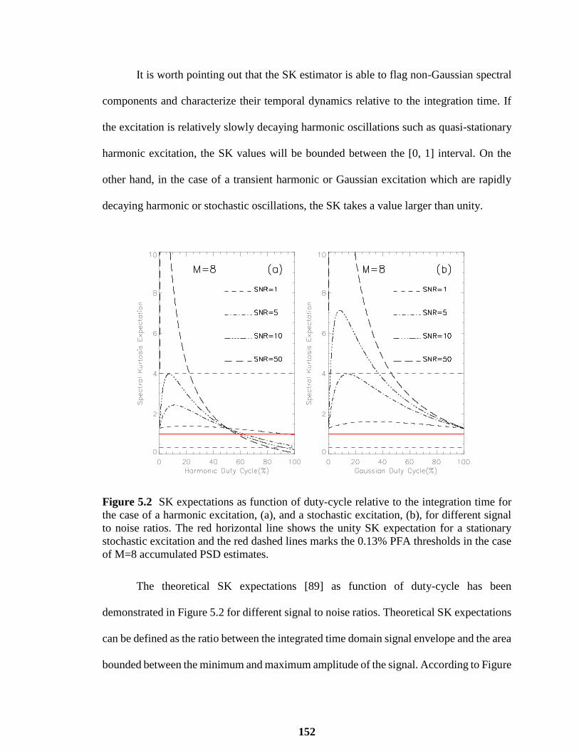
152
It is worth pointing out that the SK estimator is able to flag non-Gaussian spectral
components and characterize their temporal dynamics relative to the integration time. If
the excitation is relatively slowly decaying harmonic oscillations such as quasi-stationary
harmonic excitation, the SK values will be bounded between the [0, 1] interval. On the
other hand, in the case of a transient harmonic or Gaussian excitation which are rapidly
decaying harmonic or stochastic oscillations, the SK takes a value larger than unity.
Figure 5.2 SK expectations as function of duty-cycle relative to the integration time for
the case of a harmonic excitation, (a), and a stochastic excitation, (b), for different signal
to noise ratios. The red horizontal line shows the unity SK expectation for a stationary
stochastic excitation and the red dashed lines marks the 0.13% PFA thresholds in the case
of M=8 accumulated PSD estimates.
The theoretical SK expectations [89] as function of duty-cycle has been
demonstrated in Figure 5.2 for different signal to noise ratios. Theoretical SK expectations
can be defined as the ratio between the integrated time domain signal envelope and the area
bounded between the minimum and maximum amplitude of the signal. According to Figure

153
5.2, in the case illustrated here which is sum of only M=8 consecutive PSD estimates, it
can be concluded that the ability of the SK estimator to discriminate various types of
spectral components is limited to relatively high SNR and duty-cycle harmonic system
responses. Hence, the SK estimator is potentially more efficient in detecting harmonic or
stochastic transients. Moreover, where similar plots are shown for M=1000 it has been
illustrated that with the accumulation numbers, the efficiency of the SK estimator increases
[89].
5.5.2 The Experimental Data Set
To better serve the purpose of this study, which is to provide a proof of concept for the
applicability of the methods it proposes, dynamic response of the concrete box bridge due
to different moving truck load scenarios and El-Centro earthquake as illustrated in Section
2.4 has been analyzed which thus allows immediate comparison between undamaged and
damaged bridge.
However, the Data from Dynamic Analysis of the bridge using Lusas Bridge
software contains only pure oscillation of the structure without any background noise,
which is not identical to a real dataset collected from sensors. Thus, to demonstrate the full
potential of the SK analysis, results presented in this section are based on a hybrid
simulation in which, the original data streams were digitally mixed with two computer
generated narrow band harmonic signals. For instance, Figure 5.3 presents the data
obtained from dynamic analysis without any background noise, and Figure 5.4 shows the
data in the presence of added noise based on the above mentioned assumption. It is worth
noticing that without noise, the SK estimator is flat but well above unity, while in the
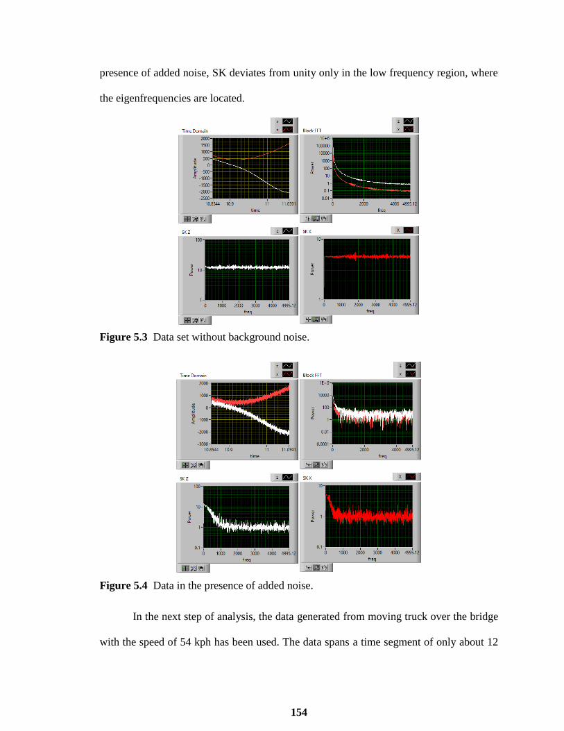
154
presence of added noise, SK deviates from unity only in the low frequency region, where
the eigenfrequencies are located.
Figure 5.3 Data set without background noise.
Figure 5.4 Data in the presence of added noise.
In the next step of analysis, the data generated from moving truck over the bridge
with the speed of 54 kph has been used. The data spans a time segment of only about 12
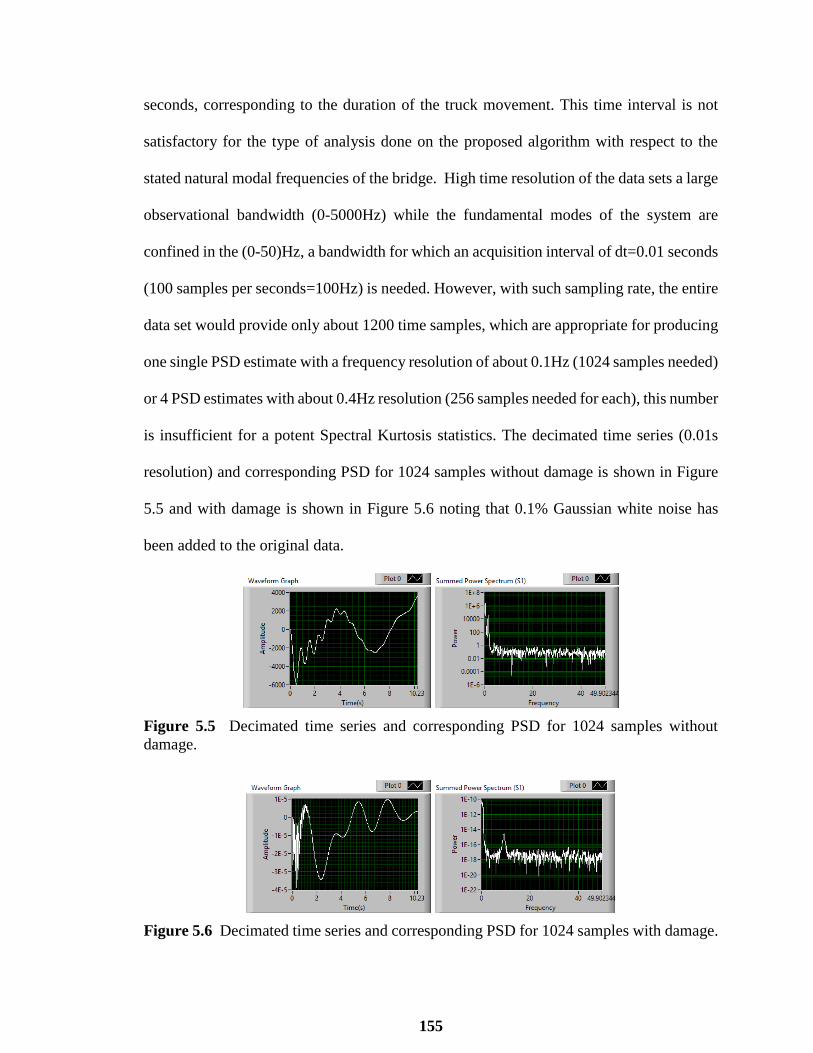
155
seconds, corresponding to the duration of the truck movement. This time interval is not
satisfactory for the type of analysis done on the proposed algorithm with respect to the
stated natural modal frequencies of the bridge. High time resolution of the data sets a large
observational bandwidth (0-5000Hz) while the fundamental modes of the system are
confined in the (0-50)Hz, a bandwidth for which an acquisition interval of dt=0.01 seconds
(100 samples per seconds=100Hz) is needed. However, with such sampling rate, the entire
data set would provide only about 1200 time samples, which are appropriate for producing
one single PSD estimate with a frequency resolution of about 0.1Hz (1024 samples needed)
or 4 PSD estimates with about 0.4Hz resolution (256 samples needed for each), this number
is insufficient for a potent Spectral Kurtosis statistics. The decimated time series (0.01s
resolution) and corresponding PSD for 1024 samples without damage is shown in Figure
5.5 and with damage is shown in Figure 5.6 noting that 0.1% Gaussian white noise has
been added to the original data.
Figure 5.5 Decimated time series and corresponding PSD for 1024 samples without
damage.
Figure 5.6 Decimated time series and corresponding PSD for 1024 samples with damage.
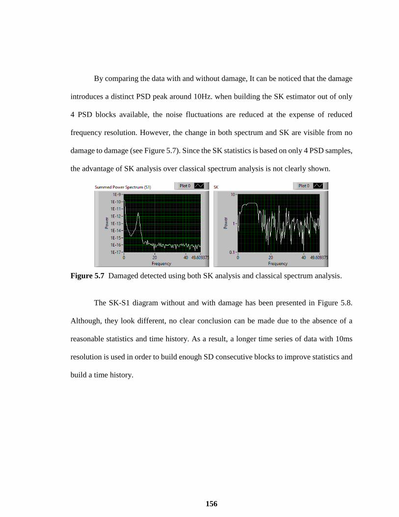
156
By comparing the data with and without damage, It can be noticed that the damage
introduces a distinct PSD peak around 10Hz. when building the SK estimator out of only
4 PSD blocks available, the noise fluctuations are reduced at the expense of reduced
frequency resolution. However, the change in both spectrum and SK are visible from no
damage to damage (see Figure 5.7). Since the SK statistics is based on only 4 PSD samples,
the advantage of SK analysis over classical spectrum analysis is not clearly shown.
Figure 5.7 Damaged detected using both SK analysis and classical spectrum analysis.
The SK-S1 diagram without and with damage has been presented in Figure 5.8.
Although, they look different, no clear conclusion can be made due to the absence of a
reasonable statistics and time history. As a result, a longer time series of data with 10ms
resolution is used in order to build enough SD consecutive blocks to improve statistics and
build a time history.

157
Figure 5.8 SK-S1 diagram without(a) and with damage(b) based on the bridge dynamic
response in X and Z directions.
For this purpose, SK analysis has been carried out on the data obtained from the
dynamic response of the bridge under Moving truck with the speed of 1.125 m/s (or 4 kph)
which provides 160 seconds time series of data and under El-Centro earthquake which
provides 60 seconds time series of data (see Section 2.4 for the dynamic analysis details).
Figure 5.9 presents the data obtained from the moving truck scenario with the speed of
1.125 m/s (or 4 kph) on both damaged and undamaged bridge. Figure 5.10 shows the data
obtained from response of the bridge due to El-Centro earthquake ground motion. In above
mentioned loading scenarios, the data from bridge without any defects shows larger
deviation from SK=1, which are not observed in the data of the bridge with defect as
expected. Utilizing these two longer time series of data from the bridge with and without
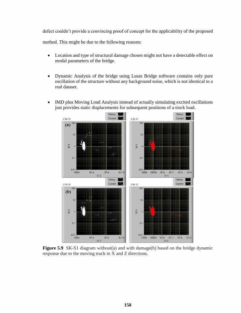
158
defect couldn’t provide a convincing proof of concept for the applicability of the proposed
method. This might be due to the following reasons:
Location and type of structural damage chosen might not have a detectable effect on
modal parameters of the bridge.
Dynamic Analysis of the bridge using Lusas Bridge software contains only pure
oscillation of the structure without any background noise, which is not identical to a
real dataset.
IMD plus Moving Load Analysis instead of actually simulating excited oscillations
just provides static displacements for subsequent positions of a truck load.
Figure 5.9 SK-S1 diagram without(a) and with damage(b) based on the bridge dynamic
response due to the moving truck in X and Z directions.
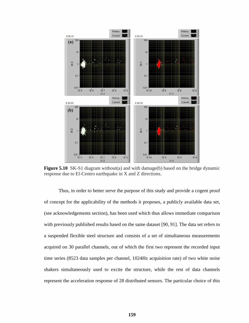
159
Figure 5.10 SK-S1 diagram without(a) and with damage(b) based on the bridge dynamic
response due to El-Centro earthquake in X and Z directions.
Thus, in order to better serve the purpose of this study and provide a cogent proof
of concept for the applicability of the methods it proposes, a publicly available data set,
(see acknowledgements section), has been used which thus allows immediate comparison
with previously published results based on the same dataset [90, 91]. The data set refers to
a suspended flexible steel structure and consists of a set of simultaneous measurements
acquired on 30 parallel channels, out of which the first two represent the recorded input
time series (8523 data samples per channel, 1024Hz acquisition rate) of two white noise
shakers simultaneously used to excite the structure, while the rest of data channels
represent the acceleration response of 28 distributed sensors. The particular choice of this
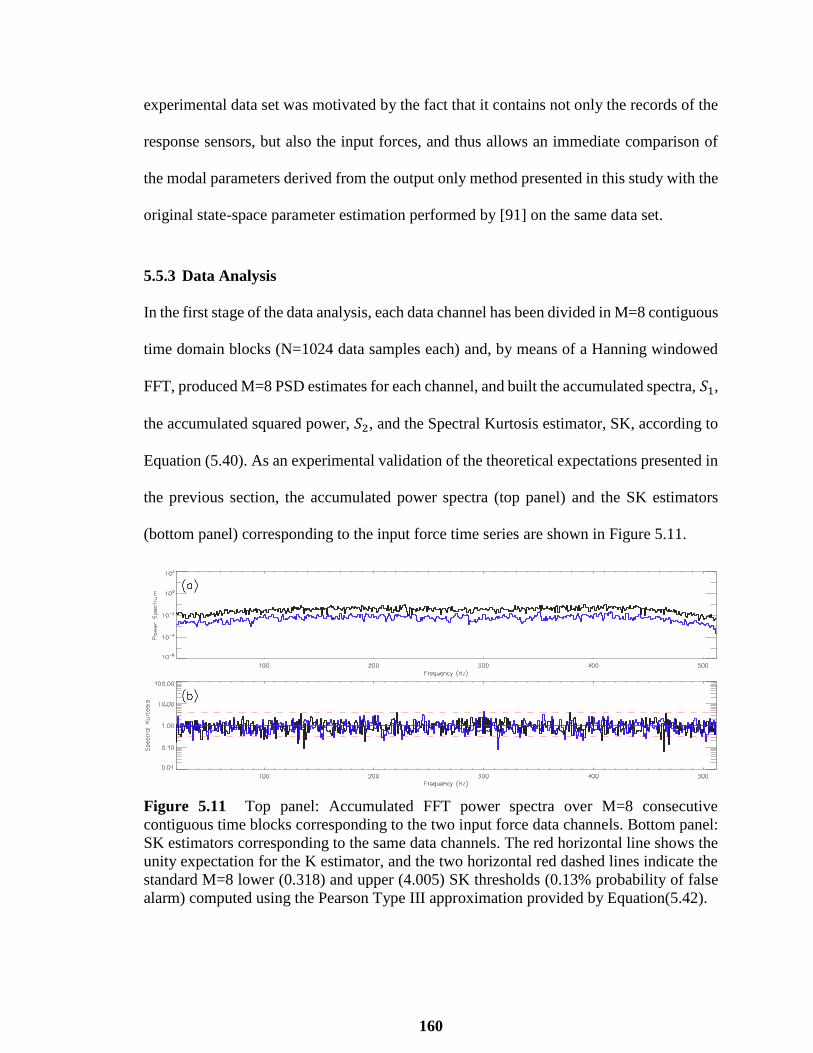
160
experimental data set was motivated by the fact that it contains not only the records of the
response sensors, but also the input forces, and thus allows an immediate comparison of
the modal parameters derived from the output only method presented in this study with the
original state-space parameter estimation performed by [91] on the same data set.
5.5.3 Data Analysis
In the first stage of the data analysis, each data channel has been divided in M=8 contiguous
time domain blocks (N=1024 data samples each) and, by means of a Hanning windowed
FFT, produced M=8 PSD estimates for each channel, and built the accumulated spectra, 𝑆1,
the accumulated squared power, 𝑆2, and the Spectral Kurtosis estimator, SK, according to
Equation (5.40). As an experimental validation of the theoretical expectations presented in
the previous section, the accumulated power spectra (top panel) and the SK estimators
(bottom panel) corresponding to the input force time series are shown in Figure 5.11.
Figure 5.11 Top panel: Accumulated FFT power spectra over M=8 consecutive
contiguous time blocks corresponding to the two input force data channels. Bottom panel:
SK estimators corresponding to the same data channels. The red horizontal line shows the
unity expectation for the K estimator, and the two horizontal red dashed lines indicate the
standard M=8 lower (0.318) and upper (4.005) SK thresholds (0.13% probability of false
alarm) computed using the Pearson Type III approximation provided by Equation(5.42).
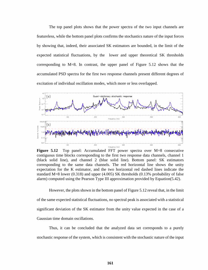
161
The top panel plots shows that the power spectra of the two input channels are
featureless, while the bottom panel plots confirms the stochastics nature of the input forces
by showing that, indeed, their associated SK estimators are bounded, in the limit of the
expected statistical fluctuations, by the lower and upper theoretical SK thresholds
corresponding to M=8. In contrast, the upper panel of Figure 5.12 shows that the
accumulated PSD spectra for the first two response channels present different degrees of
excitation of individual oscillation modes, which more or less overlapped.
Figure 5.12 Top panel: Accumulated FFT power spectra over M=8 consecutive
contiguous time blocks corresponding to the first two response data channels, channel 1
(black solid line), and channel 2 (blue solid line). Bottom panel: SK estimators
corresponding to the same data channels. The red horizontal line shows the unity
expectation for the K estimator, and the two horizontal red dashed lines indicate the
standard M=8 lower (0.318) and upper (4.005) SK thresholds (0.13% probability of false
alarm) computed using the Pearson Type III approximation provided by Equation(5.42).
However, the plots shown in the bottom panel of Figure 5.12 reveal that, in the limit
of the same expected statistical fluctuations, no spectral peak is associated with a statistical
significant deviation of the SK estimator from the unity value expected in the case of a
Gaussian time domain oscillations.
Thus, it can be concluded that the analyzed data set corresponds to a purely
stochastic response of the system, which is consistent with the stochastic nature of the input

162
forces used to excite the system. It is also worth noting that the SK estimator provides
straightforward and theoretically objective means to validate the stochastic nature of a
system response without any need to make assumptions about the unknown statistical
nature of the driving forces, which would not have been possible limiting the analysis to
the first order statistics spectral description of the data provided by the PSD estimate alone
[92].
However, due to the pure statistical nature of this particular data set to demonstrate
the full potential of the SK analysis, the subsequent results has been presented based on a
hybrid simulation in which, the original experimental data streams were digitally mixed
with two computer generated narrow band harmonic signals. Therefore, a quasi- stationary
harmonic response characterized by a relatively slow exponential decay (0.85% duty-
cycle) and harmonic transient response characterized by a relatively fast exponential decay
(0.11% duty-cycle) have been simulated.
The result of the SK analysis shown in bottom panel of Figure 5.13, which is
consistent with the theoretical expectations presented in Figure 5.2, fully demonstrates the
ability of the SK estimator objectively discriminate the deterministic or non-stationary
system responses, performance that could not have been achieved solely based on the
analysis of the spectral peaks present in the upper panel accumulated spectral power plots.
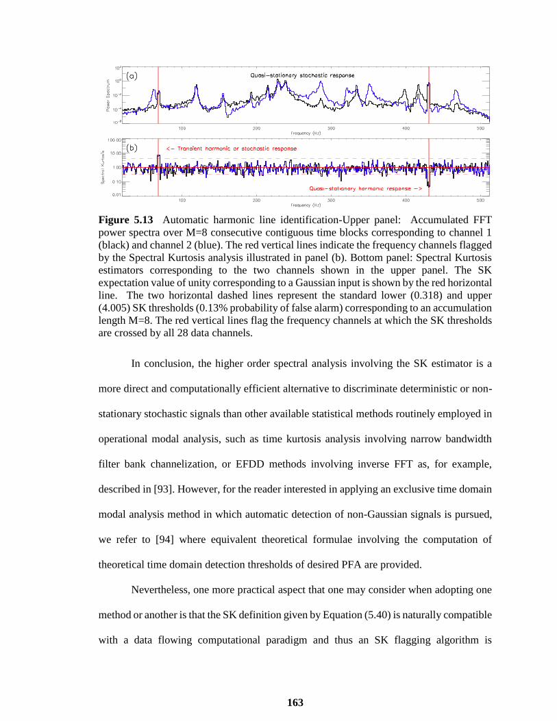
163
Figure 5.13 Automatic harmonic line identification-Upper panel: Accumulated FFT
power spectra over M=8 consecutive contiguous time blocks corresponding to channel 1
(black) and channel 2 (blue). The red vertical lines indicate the frequency channels flagged
by the Spectral Kurtosis analysis illustrated in panel (b). Bottom panel: Spectral Kurtosis
estimators corresponding to the two channels shown in the upper panel. The SK
expectation value of unity corresponding to a Gaussian input is shown by the red horizontal
line. The two horizontal dashed lines represent the standard lower (0.318) and upper
(4.005) SK thresholds (0.13% probability of false alarm) corresponding to an accumulation
length M=8. The red vertical lines flag the frequency channels at which the SK thresholds
are crossed by all 28 data channels.
In conclusion, the higher order spectral analysis involving the SK estimator is a
more direct and computationally efficient alternative to discriminate deterministic or non-
stationary stochastic signals than other available statistical methods routinely employed in
operational modal analysis, such as time kurtosis analysis involving narrow bandwidth
filter bank channelization, or EFDD methods involving inverse FFT as, for example,
described in [93]. However, for the reader interested in applying an exclusive time domain
modal analysis method in which automatic detection of non-Gaussian signals is pursued,
we refer to [94] where equivalent theoretical formulae involving the computation of
theoretical time domain detection thresholds of desired PFA are provided.
Nevertheless, one more practical aspect that one may consider when adopting one
method or another is that the SK definition given by Equation (5.40) is naturally compatible
with a data flowing computational paradigm and thus an SK flagging algorithm is

164
conceptually simple to be embedded in processors capable of real-time blind detection of
harmonic response and damage detection [88].
5.6 A Maximum Likelihood Curve Fitting Method
for Frequency Domain Decomposition
5.6.1 Theoretical Background
In this section, a new curve fitting maximum likelihood method will be demonstrated. In
which, the statistical nature of statistical fluctuations that affect power spectra obtained by
FFT has been taken into consideration. This method provides more reliable and accurate
means for mode identification and estimation of modal parameters in operational modal
analysis.
The proposed method first has been theoretically developed for the purpose of
automatic decomposition of astronomical radio spectra as a linear superposition of an
unknown number of overlapping individual spectral spikes which assumed to have
Gaussian bell shapes [95]. It is based on the assumption that the FFT of response signal to
stochastic excitation is a superposition of decaying resonant modal contributions.
Consequently, the Gaussian superposition has been replaced with a linear superposition of
𝑛 partially overlapping Lorentz spectral peaks in the original spectral decomposition
algorithm development [95].

165
1
0
12
1n
i
i
k ik
i
ss af b
c
(5.43)
being 𝑆0 the background noise level, 𝑛 the number of spectra peaks, 𝑎𝑖, 𝑏𝑖 and 𝑐𝑖
the Lorentzian parameters which are unknown and have to be determined in order to obtain
accurate estimates of the number of fundamental modes and their characteristic parameters,
𝑓0𝑖 = √𝑏𝑖2 + 𝑐𝑖
2 the natural mode frequencies, , and 𝜉𝑖 = 1/√1 + (𝑏𝑖/𝑐𝑖)2 the relative
damping ratios.
An original statistical estimator has been introduced in order to find a Maximum
Likelihood solution of such frequency domain decomposition problem, which is called
Sample to Model Ratio (SMR) [95]. For every frequency 𝑓𝑘 , it is defined as the ratio
between the accumulated power 𝑆𝑘, and the yet to be determined most likely spectral
model 𝑠𝑘, as follows:
/k k kS s
(5.44)
In the case of the true spectral model, and assuming that time domain noise
normally distributed, the SMR estimator is expected to fluctuate around unity since a

166
probability distribution function found to be a gamma distribution of unit mean and 1/M
variance,
11kMM M
k kG M e M
(5.45)
which provides the probabilities to observe a local SMR deviations above the mean,
𝑝𝑎 = 𝑝𝑟𝑜𝑏(𝜌𝑘 > 1), and below the mean 𝑝𝑏 = 𝑝𝑟𝑜𝑏(𝜌𝑘 < 1),
1 1
( ,M) ( ) ; 1 ( ,M) ( )a bp M M p M M
(5.46)
The Maximum Likelihood solution for the unknown set of free parameters may be
obtained by minimizing the negative Log Likelihood function:
0 1 1 1
1
(s , , ,c ) 2 / 1 1/N
N N N k k k k
k
a b M S s Ln s M Ln S
(5.47)

167
and the goodness of fit may be estimated by evaluating a ChiSq-like estimator associated
with the degrees of freedom of the minimization problem (number of frequency bins
minus number of free model parameters):
22
1
11
N
k
k
MN
(5.48)
The goodness of fit estimator defined by Equation (5.48) has a probability to be
equal or larger than the observed one given by:
1
2 2( ) ,3 2 3 2 3 2
M M Mp
M M M
(5.49)
which reduces to a standard ChiSq probability only in the limit of a large M.
To address the well-known problem of computational sensitivity of the ML
minimization problem relative to the initial conditions, a more robust standard least-square
fit in a first stage can be performed using the statistically justified weights
𝑤𝑘 = (𝑀 + 1)/𝑆𝑘2, followed by a second stage ML minimization of Equation (5.47).
However, it is necessary to estimate the true number of individual modes 𝑛 in order to have
a well-stated ML problem which is also a free parameter that has to be determined from

168
the data. As an alternative to the peak-picking method, which is biased in principle and not
well-suited for an automated frequency domain decomposition algorithm, an additional
statistical estimator, 𝜂𝑎, defined as the mean of a given number of systematic SMR
deviations. In a compact region of the observed spectrum, SMR deviations are all above
unity and situation that may indicate a missing peak in the model function used to fit the
spectrum [95]. Hence, if the true number of spectral peaks is correctly estimated, there is
practically a null probability for such compact regions to deviate from unity more than a
hard limit that can be expressed solely in terms of the accumulation length 𝑀 and the
number of spectral points belonging to such region [92].
5.6.2 Algorithm Implementation and Validation
To demonstrate the suitability of the curve fitting algorithm described above for operational
modal analysis, the same division of the 28 response data channels in M contiguous time
domain blocks has been used, and built the 28×28 accumulated cross-correlation matrix
associated with the response data channels. Following a standard FDD approach [96], the
singular value decomposition (SVD) of the cross-correlation matrix was performed, and
thus 28 SVD spectra was obtained, those being associated with the largest 6 SVD values
being shown on the top panel of Figure 5.14, which indicate that the dominant SVD
spectrum (thick black line) contains all spectral peaks visible on least one of the channel-
based power spectra like those displayed in Figure 5.11 (a).
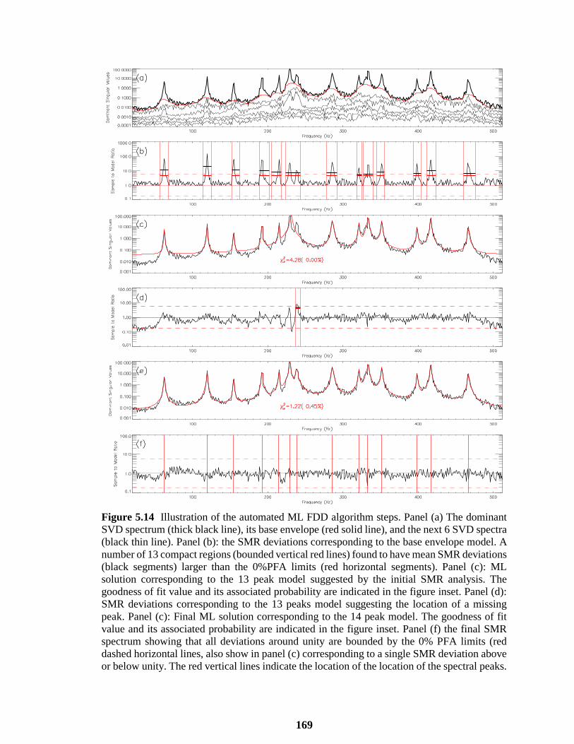
169
Figure 5.14 Illustration of the automated ML FDD algorithm steps. Panel (a) The dominant
SVD spectrum (thick black line), its base envelope (red solid line), and the next 6 SVD spectra
(black thin line). Panel (b): the SMR deviations corresponding to the base envelope model. A
number of 13 compact regions (bounded vertical red lines) found to have mean SMR deviations
(black segments) larger than the 0%PFA limits (red horizontal segments). Panel (c): ML
solution corresponding to the 13 peak model suggested by the initial SMR analysis. The
goodness of fit value and its associated probability are indicated in the figure inset. Panel (d):
SMR deviations corresponding to the 13 peaks model suggesting the location of a missing
peak. Panel (c): Final ML solution corresponding to the 14 peak model. The goodness of fit
value and its associated probability are indicated in the figure inset. Panel (f) the final SMR
spectrum showing that all deviations around unity are bounded by the 0% PFA limits (red
dashed horizontal lines, also show in panel (c) corresponding to a single SMR deviation above
or below unity. The red vertical lines indicate the location of the location of the spectral peaks.

170
In the next step of analysis, the dominant SVD spectrum has been divided by the
lower spectral envelope (red solid line), which is considered as the first order
approximation of the spectral model, and produce the SMR spectrum shown on Figure 5.14
panel (b). The SMR spectrum is then used to automatically flag 13 distinct compact regions
(delimited by vertical red lines) for which the averaged SMR deviations (horizontal black
solid segments) were found to be larger than the 0%PFA limits (horizontal red solid
segments), which were computed for M=8 and their lengths l (according to the formulae
provided by [95]). The lower and upper ~0% PFA limits for any single SMR deviation
(region of l=1) are indicated for reference by dashed horizontal red lines in Figure 5.14 (b).
By visual comparison of Figure 5.14 (a) and (b) it can be noticed that 12 of the 14 SVD
peaks are clearly associated with a distinct SMR compact region, except for two partially
overlapped peaks around 230Hz, which consistently correspond to the same compact SMR
region.
In the next step of the algorithm, a model function comprising a flat 𝑠0 background
and 13 peaks (Equation (5.43)) is constructed, the initial Lorentzian guess parameters are
set to values consistent with the SMR regions, and the minimization of log-likelihood
function defined by Equation (5.47) is performed in order to obtain the ML solution (red
continuous line) illustrated in of Figure 5.14(c). In the plot inset we show the associated
goodness of fit estimator 𝜒𝜈2 = 4.28, which correspond to a 0% probability to observe a
larger value for the existent model, which is an indication of a poor fit, conclusion
consistent with the fact that the automatically generated 13 peaks spectral model actually
missed one of the true peaks of the SVD spectrum.

171
In the next step of the algorithm a new SMR spectrum, shown in Figure 5.14(d), is
constructed by dividing the SVD spectrum by the 13 peaks ML solution and one missing
peak is automatically identified at the correct location, as marked by the two vertical lines.
As a consequence, the spectral model is amended by adding the missing peak and a new
log-likelihood minimization is performed to derive the solution shown in Figure 5.14(e).
As expected, the new solution is characterized by a smaller goodness of fit value,
𝜒𝜈2 = 1.22, which, according to Equation (5.49) correspond to a 0.45% probability to
observe a larger deviation for the same model and another realization of the noise
fluctuations.
As a final validation of the algorithm, we display in Figure 5.14(f) the final SMR
spectrum showing that all deviations around unity are bounded by the 0% PFA limits (red
dashed horizontal lines) corresponding to a single SMR deviation above or below unity.
For a quantitative assessment, the ML modal parameters, i.e. the natural frequencies
and relative damping ratios, are displayed in Table 5.1, where they are compared with
original modal parameters derived from the same data set by using a Multivariable
Subspace Identification (MOESP) estimation method involving both the input and output
channels [90].
The quantitative comparison with the references values shows an excellent
agreement in terms of natural frequency estimations (less than 1% relative difference),
while the relative damping ratios disagree more, with a general trend of the ML damping
ratios being overestimated relative to the MOESP values. The ML method, however, fails
to resolve the 156.45 Hz mode, which may be just an intrinsic limitation of any OMA
method lacking full information about the true input forces.

172
Table 5.1 Comparison Between the Modal Parameters Estimated by Maximum-
Likelihood Fit of the Dominant Singular Value Decomposition Spectrum with the Original
State-space Estimates Obtained by [90].
Natural Frequency Estimates (Hz) Damping Ratio Estimates (%)
Reference ML fit Relative difference (%) Reference ML fit Relative difference (%)
1 62.22 62.36 0.23 0.67 0.92 38.00
2 118.90 118.90 0.00 0.20 0.44 118.54
3 154.49 154.53 0.03 0.08 0.15 81.93
156.45 0.25
4 192.44 192.45 0.01 0.22 0.22 -1.57
5 214.94 214.68 -0.12 0.23 0.17 -26.87
6 229.35 229.11 -0.11 0.11 0.27 145.64
7 239.33 238.54 -0.33 0.26 0.47 81.74
8 286.79 285.84 -0.33 0.19 0.35 84.44
9 321.14 321.00 -0.04 0.15 0.20 36.15
10 333.98 332.96 -0.31 0.24 0.33 35.96
11 352.33 351.24 -0.31 0.26 0.19 -27.54
12 398.18 398.36 0.05 0.17 0.16 -8.34
13 417.59 416.63 -0.23 0.13 0.16 23.84
14 467.49 466.92 -0.12 0.16 0.19 16.23
Note: The outlined row corresponds to a spectral mode not resolved by the ML fitting method.
5.7 Conclusions
Experimental methods based on modal analysis under ambient vibrational excitation are
often employed to detect structural damages of mechanical systems. An extensive literature
review has been crucial for the identification of effective procedures of operational modal
analysis. The mathematical background and the main characteristics of the methods have
been deeply discussed in this chapter. Many of the frequency domain methods, such as

173
Basic Frequency Domain (BFD), Frequency Domain Decomposition (FFD), or Enhanced
Frequency Domain Decomposition (EFFD), use as first step a Fast Fourier Transform
(FFT) estimate of the power spectral density (PSD) associated with the response of the
system. In this chapter, it is shown that higher order statistical estimators such as Spectral
Kurtosis (SK) and Sample to Model Ratio (SMR) can be successfully employed not only
to more reliably discriminate the response of the system against the ambient noise
fluctuations, but also to better identify and separate contributions from closely spaced
individual modes. Moreover, it is shown that a SMR-based Maximum Likelihood curve
fitting algorithm improve the accuracy of the spectral shape and location of the individual
modes and, when combined with the SK analysis, it provides efficient means to categorize
such individual spectral components according to their temporal dynamics as harmonic or
stochastic system responses to unknown ambient excitations.

174
CHAPTER 6
CONCLUSIONS AND FUTURE WORK
6.1 Conclusions
Structural Health Monitoring, damage detection and localization of bridges using Wireless
Sensor Networks (WSN) are studied in this thesis. This research is motivated by the need
to improve the efficiency and accuracy of the current highway bridge inspection and
maintenance practice. The application of SHM on bridge structures will enable the
condition of the bridge to be constantly monitored and prevent unnecessary costly and
emergent maintenance. To this end, wireless monitoring systems provide a new approach
and enhace the use of current SMH systems by maximizing the lifetime of the system, the
accuracy of the sensed data, and the system reliability, and minimizing the system cost.
An extensive literature review of Structural Health Monitoring, Vibration-Based
Damaged Detection techniques and Operational Modal Analysis is first provided. By
comparing the relative merits and shortcomings of the various methods proposed to date,
promising techniques and areas that need further research are identified.
Finite Element Analysis (FEA) has been carried out using LUSAS Bridge Plus
software to simulate the behavior of a scaled down reinforced concrete frame, 3-span
bridge and an in-service 6-span precast segmental box girder bridge. Model development
for each structure is demonstrated. Element types used in the models are covered along
with the constitutive assumptions and parameters for the various materials in each section.
Besides, Geometry of the models, loading and boundary conditions are illustrated. The
mode shapes obtained from eigenvalue frequency analysis are presented. For the 3-span
bridge Moving Load analysis has been carried out using the IMDPlus facility and Seismic

175
Response of the bridge under El Centro earthquake ground motion is presented.
Furthermore, Static and Dynamic Finite Element analysis of the 6-Span Precast Segmental
Box Girder Bridge has been carried out. Finite Element Analysis results for each model
thoroughly demonstrated in each section. The Finite Element Analysis performed in this
chapter is employed in the next chapters.
A preliminary study in designing and setting up a test-bed for the research on SHM
of bridges utilizing Wireless Sensor Networks is presented in chapter 3. The test-bed
encompasses the physical model and FE model of a scaled down reinforced concrete frame
from chapter 2. The design and setup of the physical model are presented in detail. The
reinforced concrete frame was excited by sine excitation using the shaking table at six
different frequencies and the time history data were measured using five MEMS
accelerometers with the help of wireless sensing system. To show overall data quality of
the measured acceleration, a sample time histories of 15 seconds are provided. It is
concluded from the plot results that the developed wireless sensing system is capable of
measuring the dynamic response of the RC frame structure with reliable precision level.
Designing a SHM system is a systematic work integrating various expertise. In
chapter 4, first the design criteria of SHM for a large-scale bridge is outlined. The
commonly used types of sensory systems is then introduced. As a new and potentially
promising sensing, transmission and monitoring system method, wireless monitoring is
specially described in this chapter. Moreover, design and realization of power harvesting
and power usage optimization for self-sustainable operation of SMH monitoring systems
using wireless sensor networks is briefly discussed. Finally, the long-term Structural
Health Monitoring System using Wireless Sensor Networks (WSNs) for the in-service

176
highway bridge is introduced. The results obtained from the FEA has been utilized to
determine sensor locations and measurement types and could effectively minimize the
number of sensors, data for transmission, and volume of data for processing.
Experimental methods based on modal analysis under ambient vibrational
excitation are often employed to detect structural damages of mechanical systems.. Many
of the frequency domain methods, such as Basic Frequency Domain (BFD), Frequency
Domain Decomposition (FFD), or Enhanced Frequency Domain Decomposition (EFFD),
use as first step a Fast Fourier Transform (FFT) estimate of the power spectral density
(PSD) associated with the response of the system. In chapter 5, it is shown that higher order
statistical estimators such as Spectral Kurtosis (SK) and Sample to Model Ratio (SMR)
can be successfully employed not only to more reliably discriminate the response of the
system against the ambient noise fluctuations, but also to better identify and separate
contributions from closely spaced individual modes. Moreover, it is shown that a SMR-
based Maximum Likelihood curve fitting algorithm improve the accuracy of the spectral
shape and location of the individual modes and, when combined with the SK analysis, it
provides efficient means to categorize such individual spectral components according to
their temporal dynamics as harmonic or stochastic system responses to unknown ambient
excitations.
6.2 Recommendations for Future Work
This study has demonstrated the potential of using wireless sensor technology for long term
and real-time structural health monitoring and post-event damage detection. Meanwhile,
this study also identified key issues and tasks, as listed below, that must be addressed before
the proposed damage detection algorithm and wireless monitoring system can be applied

177
to the new stadium that State of Qatar will build in preparation for the 2022 World Cup.
The research on structural health monitoring using WSNs, damage identification and
sensor placement process is still a novel field of study, especially for long term monitoring
of bridges. Based on the research in this study, the following tasks and topics are
recommended for future work:
Validating the accuracy of results obtained from Finite Element Analysis of the RC
frame by using lab-scale experimental results.
Identifying modal parameters of the frame such as: natural frequencies, modal
shapes and damping ratios.
Improving the initial FE model utilizing Finite Element Model updating techniques.
Development of different type of damage cases in the form of saw cuts perpendicular
to the longitudinal axis of the beam. Comparing modal test results of the damaged
frames to the updated FE model for the subsequent studies of damage detection.
Deployment of proposed Structural Health Monitoring system using Wireless
Sensor Networks on the in-service highway bridge located in Qatar and Identifying
modal parameters of the bridge.
Applying the proposed damage detection and localization technique proposed in this
study to the in-service highway bridge for long term monitoring.
Performing FE model updating to provide the basis for the future use of the updated
model to predict the capacity and remaining life of the aforementioned bridge.

178
APPENDIX A
CONSTRUCTION OF REINFORCED CONCRETE FRAME
The RC frame used for all the lab experiments mentioned above was constructed at
University of Qatar. The pictures below show the step by step building of the frame from
assembling the form-work to curing. The frame was cast and cured under standard
conditions. It was design to have dimension to match the test bed of shaking table along
with frame legs to be able to fix it on the shaking table. The frame was cured in a steam
room 28 days after pouring.
Figure A.1 Reinforcement assembly.
Figure A.2 The wood works and reinforcement for the RC frame.
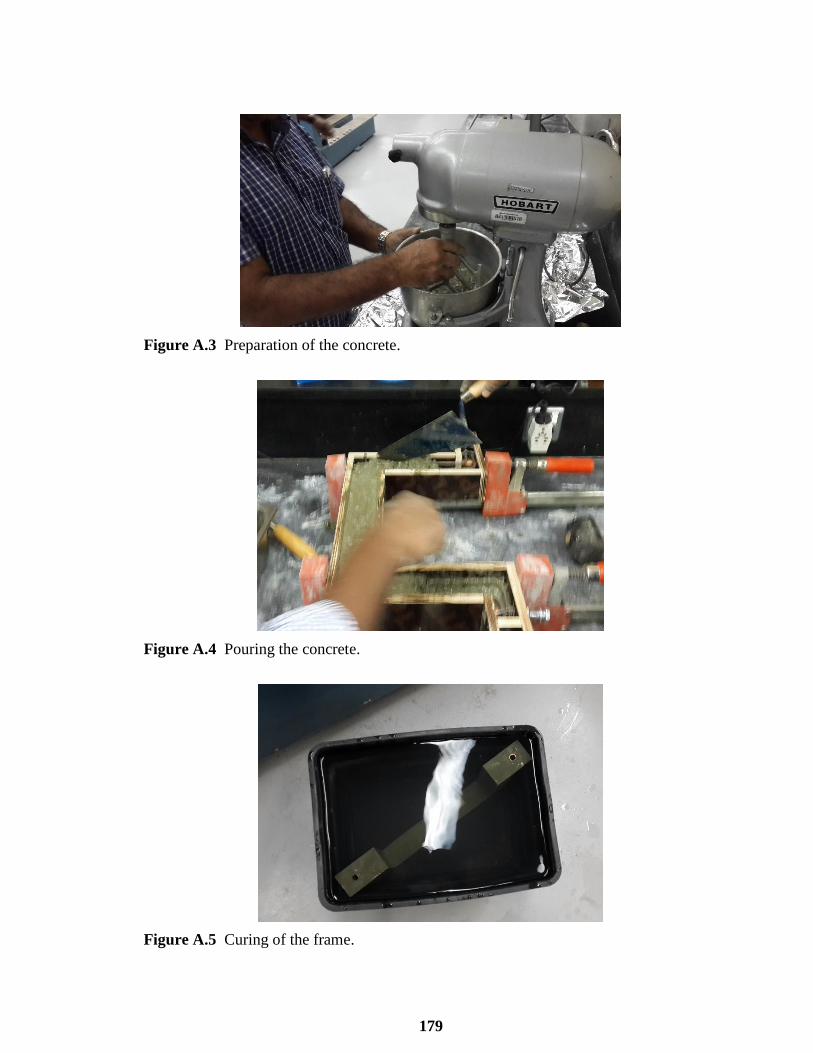
179
Figure A.3 Preparation of the concrete.
Figure A.4 Pouring the concrete.
Figure A.5 Curing of the frame.
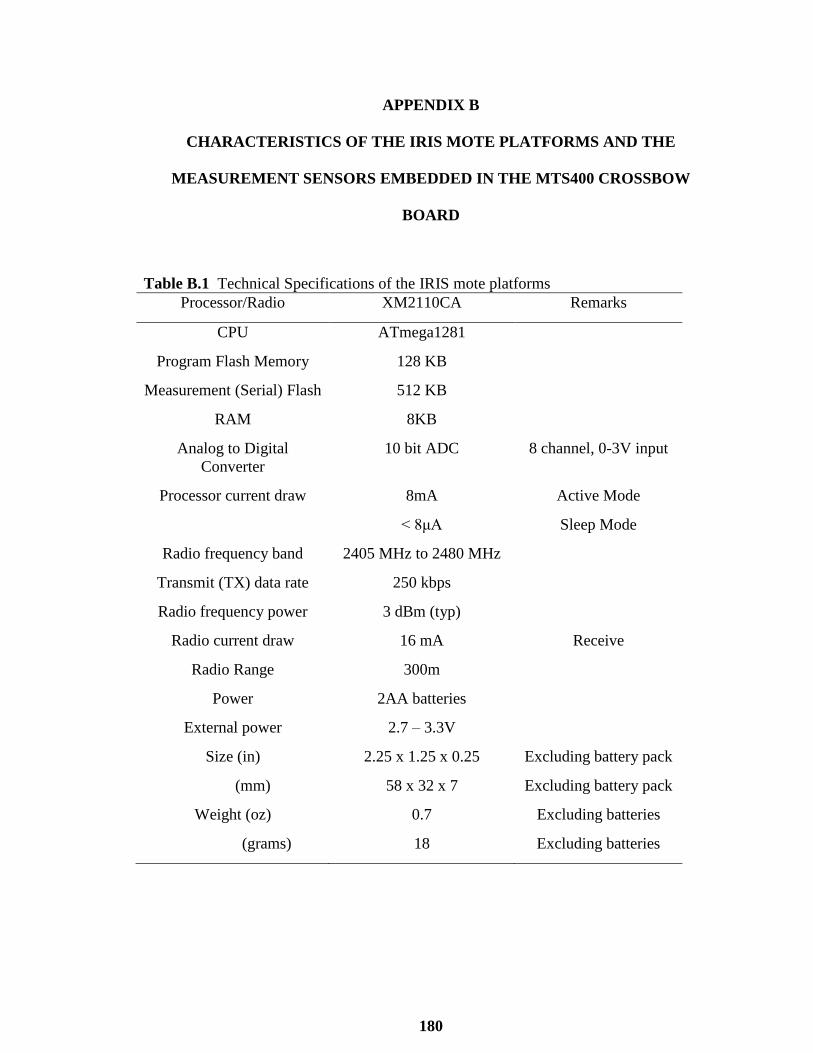
180
APPENDIX B
CHARACTERISTICS OF THE IRIS MOTE PLATFORMS AND THE
MEASUREMENT SENSORS EMBEDDED IN THE MTS400 CROSSBOW
BOARD
Table B.1 Technical Specifications of the IRIS mote platforms
Processor/Radio XM2110CA Remarks
CPU ATmega1281
Program Flash Memory 128 KB
Measurement (Serial) Flash 512 KB
RAM 8KB
Analog to Digital
Converter
10 bit ADC 8 channel, 0-3V input
Processor current draw 8mA
< 8μA
Active Mode
Sleep Mode
Radio frequency band 2405 MHz to 2480 MHz
Transmit (TX) data rate 250 kbps
Radio frequency power 3 dBm (typ)
Radio current draw 16 mA Receive
Radio Range 300m
Power 2AA batteries
External power 2.7 – 3.3V
Size (in) 2.25 x 1.25 x 0.25 Excluding battery pack
(mm) 58 x 32 x 7 Excluding battery pack
Weight (oz) 0.7 Excluding batteries
(grams) 18 Excluding batteries

181
Table B.2 Characteristics of the Humidity and Temperature Sensor
Table B.3 Characteristics of the Barometric Pressure and Temperature Sensor
Table B.4 Characteristics of the Light Sensor
Sensor Type Taos TSL2550
Channels Light
Range 400 – 1000 nm
Operating Range 3.6 to 2.7 volts
Interface Digital Interface
Sensor Type Sensirion SHT11
Channels Humidity Temperature
Range 0 to 100% -40ºC to 80ºC
Accuracy ±3.5% RH (typical) ±0.5ºC
Operating Range 3.6 to 2.4 volts
Interface Digital Interface
Sensor Type Intersema MS5534
Channels Pressure Temperature
Range 300 to 110 mbar -10ºC to 60ºC
Accuracy ±3.5% ±0.5ºC
Operating Range 3.6 to 2.4 volts
Interface Digital Interface

182
Table B.5 Characteristics of the Accelerometer Sensor
Sensor Type Analog Devices ADXL202JE
Channels X (ADC1), Y (ADC2)
Range ±2g
Sensitivity 167 mV/g, ±17%
Resolution 2mg (0.002g) RMS
Offset VBattery/2 ±0.4V
Operating Range 3.6 to 3.0 volts
Interface Analog Interface
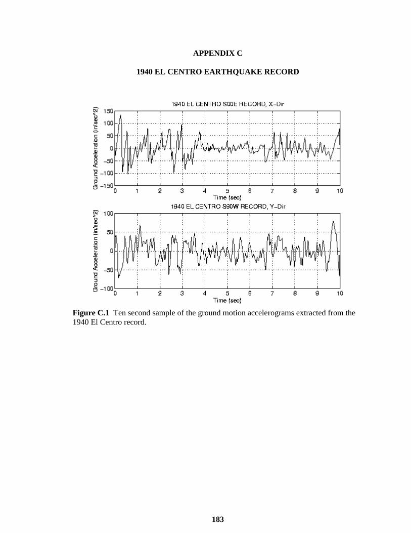
183
APPENDIX C
1940 EL CENTRO EARTHQUAKE RECORD
Figure C.1 Ten second sample of the ground motion accelerograms extracted from the
1940 El Centro record.

184
REFERENCES
[1] S. B. CHASE and J. A. LAMAN, "Dynamics and Field Testing of Bridges,"
2000.
[2] "Report Card for America’s Infrastructure," American Society of Civil Engineers,
http://www.infrastructurereportcard.org/bridges/2013.
[3] FHWA, National Bridge Inventory (NBI),
http://www.fhwa.dot.gov/bridge/nbi/defbr11.cfm2011.
[4] NBIS, "National Bridge Inspection Standards, Code of Federal Regulations," U.S.
Government Printing Office via GPO Access, 2015.
[5] M. Moore, D. Rolander, B. Graybeal, B. Phares, and G. Washer, "Highway bridge
inspection: State-of-the-Practice Study," Federal Highway Administration, ed.,
Department of Transportation, 2001.
[6] M. Moore, B. M. Phares, B. Graybeal, D. Rolander, and G. Washer, "Reliability
of visual inspection for highway bridges, volume I: Final report," 2001.
[7] S. Chase, "The Role of Sensing and Measurement in Achieving FHWA’S
Strategic Vision for Highway Infrastructure," in Sensing Issues in Civil Structural
Health Monitoring, F. Ansari, Ed., ed: Springer Netherlands, 2005, pp. 23-32.
[8] C. R. Farrar and K. Worden, "An introduction to structural health monitoring,"
Philosophical Transactions of the Royal Society A: Mathematical, Physical and
Engineering Sciences, vol. 365, pp. 303-315, 2007.
185
[9] B. F. Spencer Jr and S. Cho, "Wireless smart sensor technology for monitoring
civil infrastructure: technological developments and full-scale applications," in
Proceedings of World Congress on Advances in Structural Engineering and
Mechanics, Seoul, Korea, 2011, pp. 18-23.
[10] S. W. Doebling, C. R. Farrar, M. B. Prime, and D. W. Shevitz, "Damage
Identification and Health Monitoring of Structural and Mechanical Systems from
Changes in Their Vibration Characteristics: A Literature Review," Los Alamos
National Laboratory LA-13070-MS, 1996.
[11] H. Sohn, C. R. Farrar, F. M. Hemez, D. D. Shunk, D. W. Stinemates, B. R.
Nadler, et al., A review of structural health monitoring literature: 1996-2001: Los
Alamos National Laboratory Los Alamos, NM, 2004.
[12] D. J. Ewins, Modal testing: theory, practice and application vol. 2.
[13] C. Rainieri and G. Fabbrocino, Operational Modal Analysis of Civil Engineering
Structures: Springer, 2014.
[14] E. Parloo, P. Verboven, P. Guillaume, and M. Van Overmeire, "Force
identification by means of in-operation modal models," Journal of Sound and
Vibration, vol. 262, pp. 161-173, 2003.
[15] C. R. Farrar and K. Worden, Structural health monitoring: a machine learning
perspective: John Wiley & Sons, 2012.
[16] A. Deraemaeker, E. Reynders, G. De Roeck, and J. Kullaa, "Vibration-based
structural health monitoring using output-only measurements under changing
environment," Mechanical systems and signal processing, vol. 22, pp. 34-56,
2008.
[17] F. Magalhães, A. Cunha, and E. Caetano, "Vibration based structural health
monitoring of an arch bridge: from automated OMA to damage detection,"
Mechanical Systems and Signal Processing, vol. 28, pp. 212-228, 2012.

186
[18] "LUSAS Bridge Case Studies," http://www.lusas.com/case/bridge/index.html,
Sept. 25, 2014.
[19] K.-J. Bathe, Finite element procedures: Klaus-Jurgen Bathe, 2006.
[20] S. P. Shah, Fracture mechanics of concrete: applications of fracture mechanics to
concrete, rock and other quasi-brittle materials: John Wiley & Sons, 1995.
[21] M. Bangash, "Concrete and concrete structures: numerical modelling and
applications," 1989.
[22] "Crossbow Wireless Sensors Network," http://www.moog-crossbow.com, Apr. 1,
2015.
[23] J. M. Brownjohn and T.-C. Pan, "Identifying loading and response mechanisms
from ten years of performance monitoring of a tall building," Journal of
performance of constructed facilities, vol. 22, pp. 24-34, 2008.
[24] L. Sun, Z. Sun, D. Dan, and Q. Zhang, "Large-span bridge and their health
monitoring systems in China," in Proceeding of 2007 International Symposium on
Integrated Life-Cycle Design and Management of Infrastructure, 2007, pp. 79-95.
[25] J. Ko and Y. Ni, "Technology developments in structural health monitoring of
large-scale bridges," Engineering structures, vol. 27, pp. 1715-1725, 2005.
[26] S.-P. Chang, J. Yee, and J. Lee, "Necessity of the bridge health monitoring system
to mitigate natural and man-made disasters," Structure and Infrastructure
Engineering, vol. 5, pp. 173-197, 2009.
[27] Y. Ni, K. Wong, and Y. Xia, "Health checks through landmark bridges to sky-
high structures," Advances in Structural Engineering, vol. 14, pp. 103-119, 2011.
[28] Y. Xia, Y. q. Ni, P. Zhang, W. y. Liao, and J. m. Ko, "Stress development of a
supertall structure during construction: Field monitoring and numerical analysis,"

187
Computer‐Aided Civil and Infrastructure Engineering, vol. 26, pp. 542-559,
2011.
[29] A. E. Aktan, F. N. Catbas, K. A. Grimmelsman, and M. Pervizpour,
"Development of a model health monitoring guide for major bridges," Report
submitted to: Federal Highway Administration Research and Development, 2002.
[30] B. Hofmann-Wellenhof, H. Lichtenegger, and J. Collins, Global positioning
system: theory and practice: Springer Science & Business Media, 2012.
[31] J. R. Casas and P. J. Cruz, "Fiber optic sensors for bridge monitoring," Journal of
Bridge Engineering, vol. 8, pp. 362-373, 2003.
[32] J. M. Seim, E. Udd, W. L. Schulz, and H. M. Laylor, "Health monitoring of an
Oregon historical bridge with fiber grating strain sensors," in 1999 Symposium on
Smart Structures and Materials, 1999, pp. 128-134.
[33] Y. Ni, Y. Xia, W. Liao, and J. Ko, "Technology innovation in developing the
structural health monitoring system for Guangzhou New TV Tower," Structural
Control and Health Monitoring, vol. 16, pp. 73-98, 2009.
[34] T. S. Austin, M. M. Singh, P. J. Gregson, J. P. Dakin, and P. M. Powell, "Damage
assessment in hybrid laminates using an array of embedded fiber optic sensors,"
in 1999 Symposium on Smart Structures and Materials, 1999, pp. 281-288.
[35] E. I. Cohen, S. A. Mastro, C. P. Nemarich, J. F. Korczynski Jr, A. W. Jarrett, and
W. C. Jones, "Recent developments in the use of plastic optical fiber for an
embedded wear sensor," in 1999 Symposium on Smart Structures and Materials,
1999, pp. 256-267.
[36] Y.-L. Lo and F.-Y. Shaw, "Development of corrosion sensors using a single-pitch
Bragg grating fiber with temperature compensations," in 5th Annual International
Symposium on Smart Structures and Materials, 1998, pp. 64-72.
[37] S. Vurpillot, N. Casanova, D. Inaudi, and P. Kronenberg, "Bridge spatial
displacement monitoring with 100 fiber optic deformation sensors: Sensors

188
network and preliminary results," in Smart Structures and Materials' 97, 1997,
pp. 51-57.
[38] A. Stewart, G. Carman, and L. Richards, "Health monitoring technique for
composite materials utilizing embedded thermal fiber optic sensors," Journal of
composite materials, vol. 39, pp. 199-213, 2005.
[39] R. Sun, Z. Sun, and L. Sun, "Design and performance tests of a FBG-based
accelerometer for Structural Vibration Monitoring," in The Proceeding of 4th
China-Japan-US Symposium on Structural Control and Monitoring, 2006.
[40] Y. L. Xu and Y. Xia, Structural health monitoring of long-span suspension
bridges: CRC Press, 2011.
[41] K. RHKJM and K. Pister, "Mobile networking for smart dust," in ACM/IEEE
International Conference on Mobile Computing and Networking (MobiCom 99),
Seattle, 1999.
[42] R. M. Kling, "Intel mote: an enhanced sensor network node," in Int’l Workshop
on Advanced Sensors, Structural Health Monitoring, and Smart Structures, 2003,
pp. 12-17.
[43] R. M. Kling, "Intel motes: advanced sensor network platforms and applications,"
in Microwave Symposium Digest, 2005 IEEE MTT-S International, 2005, p. 4 pp.
[44] I. F. Akyildiz, W. Su, Y. Sankarasubramaniam, and E. Cayirci, "Wireless sensor
networks: a survey," Computer networks, vol. 38, pp. 393-422, 2002.
[45] J. Yick, B. Mukherjee, and D. Ghosal, "Wireless sensor network survey,"
Computer networks, vol. 52, pp. 2292-2330, 2008.
[46] B. Spencer, "A study on building risk monitoring using wireless sensor network
MICA mote," in First International Conference on Structural Health Monitoring
and Intelligent Infrastructure, Japan, 2003, pp. 353-363.

189
[47] M. Ruiz-Sandoval, T. Nagayama, and B. Spencer Jr, "Sensor development using
Berkeley Mote platform," Journal of Earthquake Engineering, vol. 10, pp. 289-
309, 2006.
[48] J. A. Rice and B. Spencer Jr, "Structural health monitoring sensor development
for the Imote2 platform," in The 15th International Symposium on: Smart
Structures and Materials & Nondestructive Evaluation and Health Monitoring,
2008, pp. 693234-693234-12.
[49] J. P. Lynch, K. H. Law, A. S. Kiremidjian, T. W. Kenny, E. Carryer, and A.
Partridge, "The design of a wireless sensing unit for structural health monitoring,"
in Proceedings of the 3rd International Workshop on Structural Health
Monitoring, 2001, pp. 12-14.
[50] J. P. Lynch, A. Sundararajan, K. H. Law, A. S. Kiremidjian, T. W. Kenny, and E.
Carryer, "Computational core design of a wireless structural health monitoring
system," Proceedings of Advances in Structural Engineering and Mechanics
(ASEM’02), pp. 21-23, 2002.
[51] V. M. Karbhari and F. Ansari, Structural health monitoring of civil infrastructure
systems: Elsevier, 2009.
[52] S. Jang, H. Jo, S. Cho, K. Mechitov, J. A. Rice, S.-H. Sim, et al., "Structural
health monitoring of a cable-stayed bridge using smart sensor technology:
deployment and evaluation," Smart Structures and Systems, vol. 6, pp. 439-459,
2010.
[53] J. P. Lynch and K. J. Loh, "A summary review of wireless sensors and sensor
networks for structural health monitoring," Shock and Vibration Digest, vol. 38,
pp. 91-130, 2006.
[54] Y. Gao and B. F. Spencer Jr, "Structural health monitoring strategies for smart
sensor networks," Newmark Structural Engineering Laboratory. University of
Illinois at Urbana-Champaign. 1940-9826, 2008.

190
[55] R. Kling, R. Adler, J. Huang, V. Hummel, and L. Nachman, "Intel Mote‐based
sensor networks," Structural Control and Health Monitoring, vol. 12, pp. 469-
479, 2005.
[56] "ACTEL, Low-Power Flash FPGAs Handbook Igloo Handbook,"
http://www.actel.com/documents/IGLOO_HB.pdf, 2009.
[57] S. Roundy, B. P. Otis, Y.-H. Chee, J. M. Rabaey, and P. Wright, "A 1.9 GHz RF
transmit beacon using environmentally scavenged energy," optimization, vol. 4, p.
4, 2003.
[58] J. M. Brownjohn, "Assessment of structural integrity by dynamic measurements,"
University of Bristol, 1988.
[59] F. Benedettini, D. Zulli, and R. Alaggio, "Frequency-veering and mode
hybridization in arch bridges," in Proceedings of the 27th International Modal
Analysis Conference, 2009.
[60] R. Cantieni, "Experimental methods used in system identification of civil
engineering structures," in Proceedings of the International Operational Modal
Analysis Conference (IOMAC), 2005, pp. 249-260.
[61] K. Thibert, C. E. Ventura, M. Turek, and S. Guerrero, "Dynamic soil-structure
interaction study of a reinforced concrete high-rise building," in Proceedings of
the 2nd International Operational Modal Analysis Conference, 2007.
[62] Y. Tamura, A. Yoshida, L. Zhang, T. Ito, S. Nakata, and K. Sato, "Examples of
modal identification of structures in Japan by FDD and MRD techniques," in Proc
1st international operational modal analysis conference, Copenhagen, 2005.
[63] L. F. Ramos, L. Marques, P. B. Lourenço, G. De Roeck, A. Campos-Costa, and J.
Roque, "Monitoring historical masonry structures with operational modal
analysis: Two case studies," Mechanical Systems and Signal Processing, vol. 24,
pp. 1291-1305, 2010.

191
[64] R. Brincker, P. H. Kirkegaard, P. Andersen, and M. Martinez, "Damage detection
in an offshore structure," Dept. of Building Technology and Structural
Engineering, Aalborg University1994.
[65] L. B. Ibsen and M. Liingaard, "Output-only modal analysis used on new
foundation concept for offshore wind turbine," in The International Operational
Modal Analysis Conference, 2005.
[66] M. Baptista and P. Mendes, "Use of Ambient Vibration Tests for Structural
Identification: 3 Case Studies," in 1st International Operational Modal Analysis
Conference, 2005.
[67] P. Reynolds, P. Mohanty, and A. Pavic, "Use of operational modal analysis on
empty and occupied stadia structures," in 1st International Operational Modal
Analysis Conference, 2005.
[68] S.-E. Rosenow, S. Uhlenbrock, and G. Schlottmann, "Parameter extraction of ship
structures in presence of stochastic and harmonic excitations," in Proceedings of
International Operational Modal Analysis Conference, Copenhagen, Denmark,
2007.
[69] R. Brincker, P. Andersen, N. Møller, and H. Herlufsen, "Output-only Modal
Testing of a car body subject to Engine Excitation," Proc. of the 18th
International Modal Analysis Conference, San Antonio, Texas, 2000.
[70] B. Peeters, J.-S. Servaye, and J. Cock, "Truck Applications of Operational Modal
Analysis," Proceedings of The 26th IMAC, Orlando, Florida, USA, 2008.
[71] N. Møller, R. Brincker, and P. Andersen, "Modal extraction on a diesel engine in
operation," in The International Modal Analysis Conference, 2000, pp. 1845-
1851.
[72] T. Uhl, M. Petko, G. Karpiel, and A. Klepka, "Real time estimation of modal
parameters and their quality assessment," Shock and Vibration, vol. 15, pp. 299-
306, 2008.

192
[73] J. S. Bendat and A. G. Piersol, Random data: analysis and measurement
procedures vol. 729: John Wiley & Sons, 2011.
[74] W. Heylen, S. Lammens, and P. Sas, Modal Analysis Theory and Testing:
Division of Production Engineering, Machine Design and Automation, Katholieke
Universiteit Leuven, 1994.
[75] G. H. Golub and C. F. Van Loan, Matrix computations vol. 3: JHU Press, 2012.
[76] J. C. Santamarina and D. Fratta, Discrete signals and inverse problems: an
introduction for engineers and scientists: John Wiley & Sons, 2005.
[77] J. S. Bendat and A. G. Piersol, "Engineering applications of correlation and
spectral analysis," New York, Wiley-Interscience, 1980. 315 p., vol. 1, 1980.
[78] A. J. Felber, "Development of a hybrid bridge evaluation system," University of
British Columbia, 1993.
[79] B. Peeters, "System Identification and Damage Detection in Civil Engeneering,"
2000.
[80] C. Rainieri, G. Fabbrocino, and E. Cosenza, "Some remarks on experimental
estimation of damping for seismic design of civil constructions," Shock and
Vibration, vol. 17, pp. 383-395, 2010.
[81] C. Shih, Y. Tsuei, R. Allemang, and D. Brown, "Complex mode indication
function and its applications to spatial domain parameter estimation," Mechanical
Systems and Signal Processing, vol. 2, pp. 367-377, 1988.
[82] R. J. Allemang and D. L. Brown, A Correlation Coefficient for Modal Vector
Analysis, 1982.
[83] R. Brincker, L. Zhang, and P. Andersen, "Modal identification of output-only
systems using frequency domain decomposition," Smart materials and structures,
vol. 10, p. 441, 2001.

193
[84] S. Gade, N. Møller, H. Herlufsen, and H. Konstantin-Hansen, "Frequency domain
techniques for operational modal analysis," in Proceedings 1st IOMAC
Conference, 2005, pp. 26-27.
[85] J. Rodrigues, R. Brincker, and P. Andersen, "Improvement of frequency domain
output-only modal identification from the application of the random decrement
technique," in Proc. 23rd Int. Modal Analysis Conference, Deaborn, MI, 2004.
[86] N.-J. Jacobsen, P. Andersen, and R. Brincker, "Applications of frequency domain
curve-fitting in the EFDD technique," in Proceedings IMAC XXVI Conference,
2008.
[87] R. Brincker and L. Zhang, "Frequency domain decomposition revisited," in
Proceedings of the third international operational modal analysis conference.
Porto Novo, 2009.
[88] G. M. Nita and D. E. Gary, "Statistics of the spectral kurtosis estimator,"
Statistics, vol. 122, pp. 595-607, 2010.
[89] G. M. Nita, D. E. Gary, Z. Liu, G. J. Hurford, and S. M. White, "Radio Frequency
Interference Excision Using Spectral‐Domain Statistics," Publications of the
Astronomical Society of the Pacific, vol. 119, pp. 805-827, 2007.
[90] M. Abdelghani, C. T. CHOU, and M. Verhaegen, "Using subspace methods in the
identification and modal analysis of structures," in Proceedings of SPIE, the
International Society for Optical Engineering, 1997, pp. 1392-1398.
[91] M. Abdelghani, M. Basseville, and A. Benveniste, "In-operation damage
monitoring and diagnostics of vibrating structures, with applications to offshore
structures and rotating machinery," in Proceedings of SPIE, the International
Society for Optical Engineering, 1997, pp. 1815-1821.
[92] G. M. Nita, M. Mahgoub, S. Sharyatpanahi, N. Cretu, and T. M. El-Fouly,
"Higher Order Statistical Frequency Domain Decomposition for Operational
Modal Analysis," presented at the 7th International Conference on Structural
Health Monitoring of Intelligent Infrastructure, 2015.

194
[93] N.-J. Jacobsen, P. Andersen, and R. Brincker, "Eliminating the influence of
harmonic components in operational modal analysis," in Proceedings IMAC XXV
Conference, 2007.
[94] G. M. Nita and D. E. Gary, "The generalized spectral kurtosis estimator," Monthly
Notices of the Royal Astronomical Society: Letters, vol. 406, pp. L60-L64, 2010.
[95] G. M. Nita, G. D. Fleishman, D. E. Gary, W. Marin, and K. Boone, "Fitting FFT-
derived Spectra: Theory, Tool, and Application to Solar Radio Spike
Decomposition," The Astrophysical Journal, vol. 789, p. 152, 2014.
[96] R. Brincker, L. Zhang, and P. Andersen, "Modal identification from ambient
responses using frequency domain decomposition," in Proc. of the
18th‘International Modal Analysis Conference (IMAC), San Antonio, Texas, 2000.
Top Related