


Languages
Pages
Legal


STRENGTH OF DIFFERENT ANATOLIAN SANDS IN WEDGE SHEAR, TRIAXIAL SHEAR, AND SHEAR BOX TESTS
A THESIS SUBMITTED TO THE GRADUATE SCHOOL OF NATURAL AND APPLIED SCIENCES
OF THE MIDDLE EAST TECHNICAL UNIVERSITY
BY
YUSUF ERZİN
IN PARTIAL FULFILLMENT OF THE REQUIREMENTS FOR THE DEGREE OF
DOCTOR OF PHILOSOPHY
IN
THE DEPARTMENT OF CIVIL ENGINEERING
JANUARY 2004
Approval of the Graduate School of Natural and Applied Sciences. ____________________ Prof. Dr. Canan Özgen Director I certify that this thesis satisfies all the requirements as a thesis for the degree of Doctor of Philosophy. ____________________ Prof. Dr. Erdal Çokça Head of Department This is to certify that we have read this thesis and that in our opinion it is fully adequate, in scope and quality, as a thesis for the degree of Doctor of Philosophy.
________________________ __________________________
Prof. Dr. Asuman Türkmenoğlu Prof. Dr. Türker Mirata Co-Supervisor Supervisor
Examining Committee Members
Prof. Dr. Teoman Norman (Chairman) __________________________ Prof. Dr. Yıldız Wasti __________________________ Prof. Dr. Asuman Türkmenoğlu __________________________ Prof. Dr. Reşat Ulusay __________________________ Prof. Dr. Türker Mirata _________________________
ii
ABSTRACT
STRENGTH OF DIFFERENT ANATOLIAN SANDS IN WEDGE
SHEAR, TRIAXIAL SHEAR, AND SHEAR BOX TESTS
Erzin, Yusuf
Ph. D., Department of Civil Engineering
Supervisor: Prof. Dr. Türker Mirata
Co-supervisor: Prof. Dr. Asuman Türkmenoğlu
2004, 227 pages
Past studies on sands have shown that the shear strength measured in plane
strain tests was higher than that measured in triaxial tests. It was observed that this
difference changed with the friction angle φcv at constant volume related to the
mineralogical composition. In order to investigate the difference in strength
measured in the wedge shear test, which approaches the plane strain condition, in the
triaxial test, and in the shear box test, Anatolian sands were obtained from different
locations in Turkey. Mineralogical analyses, identification tests, wedge shear tests
(cylindrical wedge shear tests (cylwests) and prismatic wedge shear tests
(priswests)), triaxial tests, and shear box tests were performed on these samples.
In all shear tests, the shear strength measured was found to increase with the
inclination δ of the shear plane to the bedding planes. Thus, cylwests (δ = 60o)
iii

yielded higher values of internal friction φ by about 3.6o than priswests (δ = 30o)
under normal stresses between 17 kPa and 59 kPa. Values of φ measured in cylwests
were about 1.08 times those measured in triaxial tests (δ ≈ 65o), a figure close to the
corresponding ratio of 1.13 found by past researchers between actual plane strain and
triaxial test results. There was some indication that the difference between cylwest
and triaxial test results increased with the φcv value of the samples. With the smaller
δ values (30o and 40o), priswests yielded nearly the same φ values as those obtained
in triaxial tests under normal stresses between 20 kPa and 356 kPa.
Shear box tests (δ =0o) yielded lower values of φ than cylwests (by about
7.9o), priswests (by about 4.4o), and triaxial tests (by about 4.2o) under normal
stresses between 17 kPa and 48 kPa. It was shown that the shear strength measured
in shear box tests showed an increase when δ was increased from 30o to 60o; this
increase (about 4.2o) was of the order of the difference (about 3.6o) between priswest
(δ = 30o) and cylwest (δ = 60o) results mentioned earlier. Shear box specimens with
δ = 60o, prepared from the same batch of any sample as the corresponding cylwests,
yielded φ values very close to those obtained in cylwests.
Keywords: Angle of internal friction, peak strength, plane strain test, sand, shear box
test, shear strength, triaxial compression test, ultimate strength, wedge
shear test
iv
ÖZ
DEĞİŞİK ANADOLU KUMLARININ KAMA KESME, ÜÇ EKSENLİ
VE KESME KUTUSU DENEYLERİNDEKİ DAYANIMI
Erzin, Yusuf
Doktora, İnşaat Mühendisliği Bölümü
Tez Danışmanı: Prof. Dr. Türker Mirata
Ortak Tez Danışmanı: Prof. Dr. Asuman Türkmenoğlu
2004, 227 sayfa
Kumlar üzerinde yapılan önceki çalışmalar, düzlemsel boy değişimi
deneylerinde ölçülen kayma dayanımının üç eksenli deneylerinde ölçülenden daha
yüksek olduğunu göstermiştir. Bu farkın mineral bileşimine bağlı olan değişmez
hacimdeki kayma dayanımı açısı φcv ile değiştiği gözlenmiştir. Düzlemsel boy
değişimi koşullarına yakın olan kama kesme deneyleri ile üç eksenli deneyler ve
kesme kutusu deneylerinde ölçülen dayanımlar arasındaki farkı araştırmak amacıyla,
Türkiye’deki farklı yörelerden kum örnekleri alınmıştır. Bunlar üzerinde mineral
analizler, tanımlama deneyleri, kama kesme deneyleri (silindirsel kama kesme
deneyleri (skkd) ve prizmatik kama kesme deneyleri (pkkd)), üç eksenli deneyler ve
kesme kutusu deneyleri yapılmıştır.
Tüm kesme deneylerinde, ölçülen kayma dayanımının kayma düzlemi ile
sıkıştırma katmanları arasındaki açıyla (δ) arttığı görülmüştür. Bu nedenle, 17 kPa
ile 59 kPa arasında değişen dikey gerilmeler altında skkd (δ = 60o), pkkd
v
(δ = 30o)’den yaklaşık olarak 3.6o daha yüksek içsel sürtünme açısı φ değerleri
vermiştir. Skkd’de ölçülen φ değerleri üç eksenli deneylerde (δ ≈ 65o) ölçülenin
yaklaşık 1.08 katı olarak bulunmuştur ki bu katsayı, önceki araştırmacılarca gerçek
düzlemsel boy değişimi deneyleri ve üç eksenli deneyler arasında bulunan 1.13
değerine yakındır. Üç eksenli ve skkd sonuçları arasındaki bu farkın, örneklerin φcv
değerleriyle arttığını gösteren belirtiler gözlenmiştir. Daha küçük δ açılarıyla (30o ve
40o) yapılan pkkd, 20 kPa ile 356 kPa arasında değişen dikey gerilmeler altında, üç
eksenli deneylerden elde edilen φ değerlerine çok yakın sonuçlar vermiştir
Kesme kutusu deneyleri (δ = 0o), 17 kPa ile 48 kPa arasında değişen dikey
gerilmeler altında, skkd’den (yaklaşık olarak 7.9o), pkkd’den (yaklaşık olarak 4.4o)
ve üç eksenli deneylerden (yaklaşık olarak 4.2o) daha düşük φ değerleri vermiştir.
Kesme kutusu deneylerinde, δ açısının 30 dereceden 60 dereceye artırılmasıyla,
kayma dayanımında bir artış gözlenmiştir. Bu artış (yaklaşık olarak 4.2o) daha önce
belirtilen skkd (δ = 60o) ve pkkd (δ = 30o) sonuçları arasındaki farkla (yaklaşık
olarak 3.6o) aynı düzeydedir. Herhangi bir örneğin, skkd örneklerinin hazırlandığı
bölümünden elde edilen kesme kutusu örnekleri (δ = 60o) skkd’den bulunan
φ değerlerine çok yakın sonuçlar vermiştir.
Anahtar kelimeler: Düzlemsel boy değişimi deneyi, en yüksek dayanım, içsel
sürtünme açısı, kama kesme deneyi, kayma dayanımı, kesme
kutusu deneyi, kum, nihai dayanım, üç eksenli basınç deneyi
vi

TO MY PARENTS
vii
ACKNOWLEDGEMENTS
The subject of this thesis was suggested by Prof. Dr. Türker Mirata, and the
work has been carried out under his supervision. The author wishes to express his
sincere gratitude to Prof. Mirata for his close supervision, guidance and
encouragement throughout this study, and for correcting the manuscript; and to his
co - supervisor Prof. Dr. Asuman Türkmenoğlu for her valuable guidance during the
mineralogical analyses.
Special thanks are also extended to Prof. Dr. Teoman Norman for his
valuable help in the selection of the sites for sampling, and during the mineralogical
and particle shape analyses; and to both Prof. Norman and Prof. Dr. Yıldız Wasti for
their valuable suggestions as members of the Ph.D. progress tracking committee.
The author would also like to thank Mr. Ali Bal of the Soil Mechanics
Laboratory for his valuable help during the shear tests, Ms. İnciser Girgin for the
mineralogical analyses, Mr. Mehmet Ekinci for some of the drawings, and last but
not least, his wife and family for their endless support.
viii
TABLE OF CONTENTS
Page
ABSTRACT................................................................................................. ii
ÖZ ................................................................................................................ iv
DEDICATION ............................................................................................. vi
ACKNOWLEDGEMENTS ......................................................................... vii
TABLE OF CONTENTS ............................................................................ viii
LIST OF TABLES ....................................................................................... xiii
LIST OF FIGURES ..................................................................................... xvii
LIST OF ABBREVIATIONS AND SYMBOLS ........................................ xxv
CHAPTER 1. INTRODUCTION .............................................................................. 1
2. REVIEW OF RELEVANT LITERATURE ....................................... 4
2.1 Factors Affecting Shear Strength of Sands ................................... 4
2.1.1 Effect of Rate of Dilatation .................................................. 4
2.1.2 Effect of Initial Void Ratio .................................................. 8
2.1.3 Effect of Confining Stress ................................................... 9
2.1.4 Effect of Intermediate Principal Stress ................................ 13
2.1.5 Effect of Particle Composition ............................................ 23
2.1.5.1 Definitions .............................................................. 23
2.1.5.2 Effect of Particle Shape and Mineral Composition 26
2.1.5.3 Effect of Particle Size ............................................. 32
2.1.5.4 Effect of Gradation ................................................. 33
ix
2.2 Effect on Shear Strength of the Inclination of Shear Plane to the
Bedding Plane in Plane Strain Tests ............................................. 34
2.3 Wedge Shear Tests ....................................................................... 35
2.3.1 Calculation of Stresses and Displacements ........................ 35
2.3.1.1 Introduction ............................................................... 35
2.3.1.2 Simplified Analysis (Analysis A) ............................. 38
2.3.1.3 Average Shear Plane Analysis (Analysis B) ............ 40
2.3.1.4 True Shear Plane Analysis (Analysis C) .................. 40
2.4 Comparison of the Wedge Shear Test with the Plane Strain Test 43
3.
MINERALOGICAL AND PARTICLE SHAPE ANALYSES OF
THE SAMPLES .................................................................................. 45
3.1 Introduction ................................................................................... 45
3.2 Preparation of the Samples ........................................................... 46
3.3 Mineralogical Analyses Performed .............................................. 46
3.4 Results of Mineralogical Analyses ............................................... 47
3.5 Results of Particle Shape Analyses ............................................... 52
4. PHYSICAL AND COMPACTION PROPERTIES OF THE
SAMPLES .......................................................................................... 53
4.1 Introduction ................................................................................... 53
4.2 Sieve Analyses and Particle Breakage .......................................... 53
4.2.1 Particle Breakage during Shear ......................................... 53
4.2.2 Particle Breakage during Compaction ............................... 59
4.3 Density Tests ................................................................................ 61
4.3.1 Maximum Density Tests ..................................................... 61
4.3.2 Minimum Density Tests ..................................................... 63
4.3.2.1 Minimum Density Tests Performed by Following
the Procedure for Sands ....................................... 64
x

4.3.2.2 Minimum Density Tests Performed by Following
the Procedure for Gravelly Soils ............................ 65
4.3.2.3 Comparison of Minimum Density Test Results ..... 67
4.3.3 Determination of Dry Density / Water Content Relation
by Standard Proctor Compaction Test .................................. 67
4.4 Specific Gravity Tests ................................................................... 69
5. WEDGE SHEAR TESTS PERFORMED .......................................... 70
5.1 Cylindrical Wedge Shear Tests Performed ................................... 70
5.1.1 Introduction ......................................................................... 70
5.1.2 Calculation of Wet Mass of Each Layer ............................. 70
5.1.3 Test Procedure ................................................................... 72
5.1.4 Order of Testing Cylwest Specimens ................................. 77
5.1.5 Evaluation of Test Results .................................................. 79
5.1.6 Test Results ......................................................................... 79
5.1.7 Effect on the Cylwest Results of the Order of Testing ....... 91
5.2 Prismatic Wedge Shear Tests Performed ..................................... 92
5.2.1 Introduction ......................................................................... 92
5.2.2 Description of the Priswest Apparatus ............................... 92
5.2.3 Test Procedure .................................................................... 95
5.2.4 Order of Testing Priswest Specimens ................................ 96
5.2.5 Evaluation of the Test Results ............................................ 98
5.2.6 Test Results ......................................................................... 99
6. TRIAXIAL TESTS PERFORMED .................................................... 120
6.1 Introduction ................................................................................... 120
6.2 Test Procedure .............................................................................. 120
6.3 Order of Testing Triaxial Test Specimens .................................... 128
6.4 Test Results ................................................................................... 130
xi

7. SHEAR BOX TESTS PERFORMED ................................................ 145
7.1 Introduction ................................................................................... 145
7.2 Description of Shear Box Test Apparatus ................................... 145
7.3 Shear Box Tests Performed on Specimens Compacted Directly
in the Shear Box ............................................................................ 147
7.3.1 Test Procedure ................................................................... 147
7.3.2 Test Results ........................................................................ 151
7.4 Shear Box Tests Performed on Specimens Taken from the Shear
Plane of Samples Compacted in the Cylwest and Priswest
Moulds ........................................................................................... 157
7.4.1 Introduction ........................................................................ 157
7.4.2 Preparation of the Samples ................................................ 157
7.4.3 Test Procedure for Specimens Taken from the Shear
Plane of Samples Compacted in the Cylwest Mould ....... 160
7.4.4 Test Procedure for Specimens Taken from the Shear
Plane of Samples Compacted in the Priswest Mould ........ 163
7.4.5 Results of Shear Box Tests on Specimens from the Shear
Plane of Samples Compacted in the Cylwest and Priswest
Moulds ............................................................................... 165
8. DISCUSSIONS ................................................................................... 170
8.1 Discussions of the Shear Test Results .......................................... 170
8.1.1 Shear Strength Measured in Wedge Shear and Triaxial
Shear Tests ........................................................................ 170
8.1.2 Comparison of Shear Strength Measured in Shear Box
Tests with other Test Results ............................................. 186
8.1.3 Possible Effect of Particle Crushing on Measured Relative
Density and Shear Strength ................................................ 194
xii
8.2 Comparison of the Results of the Shear Tests with Existing
Empirical Relationships............................................................. 194
8.3 Comparison of the Results of Shear Tests with the Strength
Limits Calculated by Using Stress – Dilatancy Equation ............. 197
8.3.1 Wedge Shear and Triaxial Tests ....................................... 197
8.3.2 Shear Box Tests ................................................................ 205
9. CONCLUSIONS AND RECOMMENDATIONS............................ 207
REFERENCES ............................................................................................. 210
APPENDICES A. CALCULATION OF PEAK FRICTION ANGLE φd FROM THE
VALUES OF R ............................................................................... 217
B. THE RELATION BETWEEN RELATIVE POROSITY AND
RELATIVE DENSITY .................................................................... 218
C. CALCULATION OF MARSAL’S (1967) PARTICLE
BREAKAGE FACTOR ................................................................... 220
D. EXAMINATION OF THE EFFECT ON CYLWEST RESULTS
OF THE USE OF THE DOUBLE-CUT CYLWEST MOULD
WITH NO TRIMMING................................................................................. 221
E. ESTIMATION OF CELL PRESSURES TO BE APPLIED IN
THE TRIAXIAL TEST .................................................................... 223
CURRICULUM VITAE ................................................................................. 227
xiii

LIST OF TABLES
TABLES Page
2.1 Friction angles at peak strength and at constant volume for
cohesionless soils (after Bardet, 1997) ………………….............. 9
2.2 Physical properties of the sand (after Adel, 2001) ………............. 22
2.3 Powers roundness criteria and values (after Youd, 1973) ............ 24
2.4 Physical properties of the quartz samples (after Koerner, 1970) ... 28
2.5 Composition properties of glass beads and sands (after Holubec
& D’Appolonia, 1973) …………………..............................…….
29
2.6 Physical properties of the sands (after Ueng & Chen, 2000) ......... 32
2.7 Effect of particle shape and grading on friction angle (quoted
from Sowers (1951) by Lambe & Whitman, 1979) …………....
34
3.1 Locations of the samples ……………………………….....……... 45
3.2 Specimen numbers for mineralogical analyses ………….............. 47
3.3 Mineralogical composition of sample A ………………….......…. 48
3.4 Details and relative contributions to strength of ingredients in
Table 3.3 for sample A ………………………………………....... 48
3.5 Mineralogical composition of sample B …………….......………. 48
3.6 Details and relative contributions to strength of ingredients in
Table 3.5 for sample B ………………………………………....... 49
3.7 Mineralogical composition of sample C ……………………........ 49
3.8 Details and relative contributions to strength of ingredients in
Table 3.7 for sample C ...................……………………………… 49
3.9 Mineralogical composition of sample D ………………….......…. 50
xiv
3.10 Details and relative contributions to strength of ingredients in
Table 3.9 for sample D .………………………………………...... 50
3.11 Mineralogical composition of sample E ………………........…… 50
3.12 Details and relative contributions to strength of ingredients in
Table 3.11 for sample E .............………………………………… 51
3.13 Mineralogical composition of sample F …………….....………... 51
3.14 Details and relative contributions to strength of ingredients in
Table 3.13 for sample F .............………………………………… 51
3.15 The results of particle shape analyses of each sample …...........… 52
4.1 Summary of the gradation and classification of samples A to F ... 54
4.2 Breakage factors calculated from the initial and final gradation of
samples A to F after different shear tests ……............................... 58
4.3 Maximum density test results ……………………….....……….. 63
4.4 Volume of specimen in the glass cylinder for different trials ........ 64
4.5 Calculation of minimum density form the procedure for sands ... 65
4.6 Mass of specimen loosely poured in the CBR mould for different
trials ……....................................................................................... 66
4.7 Calculation of minimum density from the procedure for gravelly
soils ..............………………….........……..................................... 66
4.8 The values of maximum dry density and optimum water content
for each sample .............................…………………………........ 67
4.9 Specific gravity of the samples .....……………………….....…… 69
5.1 Specimens used in the cylwests ….....………………….......……. 78
5.2 Principal features of cylwest series CA to CC on samples A to C
respectively ... ………………………............................................ 81
5.3 Principal features of cylwest series CD to CF on samples D to F
respectively .....………………………........................................... 82
5.4 Principal features of cylwest series CDH to CFH on samples D to
F respectively .....……………….................................................... 83
5.5 Results of cylwest series CA to CC ....…........………………....... 88
5.6 Results of cylwest series CD to CF ... ...…….......……………….. 89
xv

5.7 Results of cylwest series CDH to CFH .........……................……. 90
5.8 Specimens used in the priswests ……….......…………………… 97
5.9 Principal features of priswest series PA1 to PC1 on samples A to
C respectively .. …………............................................................. 100
5.10 Principal features of priswest series PA2 to PC2 on samples A to
C respectively ...………….............................................................. 101
5.11 Principal features of priswest series PD1 to PF1 on samples D to
F respectively ......…...............................……................................ 102
5.12 Principal features of priswest series PD2 to PF2 on samples D to
F respectively ..... …...............................……................................ 103
5.13 Principal features of priswest series PDH1 to PFH1 on samples
D to F respectively ......……........................................................... 104
5.14 Principal features of priswest series PDH2 to PFH2 on samples
D to F respectively .. ………......................................................... 105
5.15 Results of the priswests performed on samples A and B
at the lower density .………………………………………...…… 115
5.16 Results of the priswests performed on samples C and D
at the lower density .……………………………………………... 116
5.17 Results of the priswests performed on samples E and F at the
lower density ………………………….......………………......… 117
5.18 Results of the priswests performed on samples D and E at the
higher density .…………………..............……………………….. 118
5.19 Results of the priswests performed on sample F at the higher
density ............................................................................................ 119
6.1 Specimens used in the triaxial tests ………….............................. 129
6.2 Results of triaxial test series TA on sample A ….......................... 136
6.3 Results of triaxial test series TB on sample B …........................... 137
6.4 Results of triaxial test series TC on sample C ….......................... 138
6.5 Results of triaxial test series TD on sample D ….......................... 139
6.6 Results of triaxial test series TE on sample E …........................... 140
6.7 Results of triaxial test series TF on sample F ................................ 141
xvi

6.8 Results of triaxial test series TDH on sample D ............................ 142
6.9 Results of triaxial test series TEH on sample E ............................. 143
6.10 Results of triaxial test series TFH on sample F .…........................ 144
7.1 Results of shear box test series SA to SC …….............................. 155
7.2 Results of shear box test series SD to SF ……............................. 156
7.3 Results of shear box test series SBC to SFC ................................. 166
7.4 Results of shear box test series SBP to SFP …............................. 167
8.1 Summary of shear tests for sample A to F at the lower density .... 171
8.2 Summary of shear tests for sample D to F at the higher density ... 172
8.3 Peak friction angles obtained from the cylwests, priswests,
and triaxial tests for samples A to F .……..............................…… 173
8.4 Test numbers and normal stresses of single shear tests used for
the comparisons in Figs. 8.1 to 8.5 ................................................ 177
8.5 Ultimate friction angles obtained from the cylwests, priswests,
and triaxial compression tests for samples A to F ......................... 180
8.6 Test numbers and normal stresses of single shear tests used for
the comparisons in Figs. 8.6 to 8.10 .............................................. 184
8.7 Summary of cylwests, priswests, triaxial tests, and shear box
tests for samples A to F at the lower density ……................…… 187
8.8 Test numbers and normal stresses of single shear tests used for
the comparisons in Figs. 8.11 and 8.12 .......................................... 190
8.9 Test numbers and normal stresses of single shear tests used for
the comparisons in Figs. 8.13 and 8.14 ......................................... 190
8.10 The results of additional five cylwests on specimens previously
sheared more than once for samples B to F ................................... 193
C.1 Sample calculation for Marsal’s breakage factor ........................... 220
E.1 Sample calculation for the cell pressure to be applied in the
triaxial test ...................................................................................... 226
xvii
LIST OF FIGURES
FIGURES Page
2.1 Relation between φµ and φcv (after Rowe, 1969) ......................... 6
2.2 Comparisons of φd values measured in plane strain, triaxial
compression, and direct shear tests with theoretical peak
strength limits (after Rowe, 1969) ............................................... 7
2.3 Results of drained tests on Ham River sand (after Bishop, 1966) 11
2.4 Variation of the peak angle of friction with initial relative
density for Chattahoochee sand (after Hussaini, 1973) ......…… 15
2.5 Stress - strain relationship for plane strain and triaxial specimen
(σ3 = 70 kPa) (after Marachi et al., 1981) .…........….................. 16
2.6 Variations of peak angles of friction with confining pressure
(after Marachi et al., 1981) ..………….......…….................…… 17
2.7 Maximum strength under plane strain and triaxial tests (after
Schanz & Vermeer, 1996) .……………………................…….. 20
2.8 Comparison of relationships between peak angles of friction in
plane strain and triaxial tests (after Mirata & Gökalp, 1997) ......
21
2.9 Typical particles assigned to each category (after Youd, 1973) .. 25
2.10 Definitions of angularity and sphericity (after Norman, 2000(c)) 26
2.11 A visual comparison chart for roundness and sphericity (after
Norman, 2000(c)) ........................................................................ 27
2.12 Effect of particle shape on the φd value (after Holubec &
D’Appolonia, 1973) ..................................................................... 30
2.13 Effect of particle shape on the φd value (after Holubec &
D’Appolonia, 1973) ....................................................................
31
xviii

2.14 Forces, displacements and distances in simplified analysis of
cylwest showing (a) usual mode of failure, (b) and (c)
alternative modes (after Mirata, 1991; 2003(a)) .………............. 36
2.15 Effect of mould rotation on the measured values of δx and δy in
priswests (after Mirata, 1991; 2003(a)) ...………………............ 37
2.16 Pre-failure deformation of a plastic clay in cylwest (after
Mirata, 1991; 2003(a)) ......…………………………………….. 41
2.17 Plane strain test sample after failure (after Bishop, 1966)........... 43
4.1 Comparison of gradation of sample A at the lower density
before testing and after being sheared in cylwests .…………… 54
4.2 Comparison of gradation of sample B at the lower density
before testing and after being sheared in priswests using
the 30o mould under lower normal stresses .…………........…… 55
4.3 Comparison of gradation of sample C at the lower density
before testing and after being sheared in triaxial tests ....……… 55
4.4 Comparison of gradation of sample D at the higher density
before testing and after being sheared in cylwests ...................... 56
4.5 Comparison of gradation of sample E at the higher ensity
before testing and after being sheared in priswests using the 40o
mould under higher normal stresses .……….....................…….. 56
4.6 Comparison of gradation of sample F at the higher density
before testing and after being sheared in triaxial tests .………… 57
4.7 Original gradation of sample E and the gradations after
first and second compactions at the lower density .…........…... 60
4.8 Original gradation of sample E and the gradations after
first and second compactions at the higher density .….........…. 60
4.9 The compaction curves for samples A to F .………….......……. 68
5.1 Apparatus used for cylwests (a) modified compression
machine; (b) double-cut mould (after Gürol, 2000) .................... 71
5.2 The double-cut cylwest mould used (after Gürol (2000),
modified from Mirata, 1991; re-modified after Mirata, 2003(a)) 74
xix

5.3 Layout for cylwests performed using a 5-ton compression
machine (after Gün, 1997) ..……………………….....………… 75
5.4 Typical curves for series CA of the variation with u of (a) τ,
(b) v , (c) β, and (d) dv/du ...........................................……..... 84
5.5 Typical curves for series CDH of the variation with u of (a) τ,
(b) v , (c) β, and (d) dv/du ……….............................................. 85
5.6 The results of cylwests on samples A to F at the lower density .. 86
5.7 The results of cylwests on samples D to F at the higher density.. 87
5.8 The results of cylwest series CA ................................................. 91
5.9 Priswest set-up showing (a) box in position for placement of
sample and (b) at start of shear (adapted from Mirata, 1991;
2003(a)) .......................................................................................
93
5.10 Modified cross-beam of 20 ton priswest frame (after Mirata,
1992) ............................................................................................ 94
5.11 Typical curves for series PB1 of the variation with u of (a) τ,
(b) v , (c) β, and (d) dv/du …...….....……………….................. 106
5.12 Typical curves for series PD2 of the variation with u of (a) τ,
(b) v , (c) β, and (d) dv/du …....………...………… 107
5.13 Typical curves for series PEH1 of the variation with u of (a) τ,
(b) v , (c) β, and (d) dv/du....………………...…….................... 108
5.14 Typical curves for series PFH2 of the variation with u of (a) τ,
(b) v , (c) β, and (d) dv/du ….………………...…….................. 109
5.15 The results of priswests on samples A to F at the lower density
and lower normal stress range ….........……..........….................. 110
5.16 The results of priswests on samples A to F at the lower density
and higher normal stress range ….........……................…...…… 111
5.17 The combined results of priswests on each of samples A to F at
the lower density ....................……..…................................…… 112
xx

5.18 The results of priswest series on sample D to F at the higher
density: (a), (c), (e): lower normal stress range; (b), (d), (f):
higher normal stress range ........................................................... 113
5.19 The combined results of priswests on each of samples D to F at
the higher density ....................……..…...................................... 114
6.1 Triaxial apparatus used (adapted from Çağnan, 1990) ............... 121
6.2 Rubber membranes on the three-part split mould with special
attachment (after Gökalp, 1994) ………………………............ 122
6.3 Three-part split mould (after Gökalp, 1994) ……………......… 123
6.4 Three-part split mould with collar held gently above the rubber
membrane (after Gökalp, 1994) ..…………………………....... 124
6.5 Top view of anti-friction guide …………………………...….... 126
6.6 Layout of triaxial cell with the anti- friction guide ..…....……... 126
6.7 Typical curves for series TB of the variation of εa of
(a) (σ1-σ3)/2 and (b) εv ………........…………………………... 131
6.8 Typical curves for series TF of the variation of εa of
(a) (σ1-σ3)/2 and (b) εv ……………........…….............………… 132
6.9 Typical curves for series TDH of the variation of εa of
(a) (σ1-σ3)/2 and (b) εv .…......................................…………… 133
6.10 Typical curves for series TEH of the variation of εa of
(a) (σ1-σ3)/2 and (b) εv ……….........……….………………………………… 134
6.11 The results of the triaxial test series TA on sample A (a) at peak
strength, and (b) at ultimate strength ……..................….........… 135
6.12 The results of the triaxial test series TDH on sample D (a) at
peak strength, and (b) at ultimate strength ……......................... 135
7.1 Shear box test apparatus (after Aybak, 1988) ………….........… 146
7.2 Assembly of shear box (modified from Head (1981) by
Aybak,1988) ................................................................................ 148
7.3 Typical curves for series SA of the variation with u of (a) τ,
(b) v, and (c) β ..……………………………......……................. 152
xxi

7.4 Typical curves for series SC of the variation with u of (a) τ,
(b) v, and (c) β ............................................................................. 153
7.5 The results of shear box tests performed on specimens
compacted directly in the shear box ………........…...............….
154
7.6 Original gradation of sample B and the gradation before shear
box tests ……………………………………………................ 158
7.7 Original gradation of sample C and the gradation before shear
box tests ……………………………………………….............. 158
7.8 Original gradation of sample D and the gradation before shear
box tests …………………………………………….............…. 159
7.9 Original gradation of sample E and the gradation before shear
box tests ……………………………………………….............. 159
7.10 Original gradation of sample F and the gradation before shear
box tests ………………………………………………............... 160
7.11 Setup used for extracting shear box specimens from the cylwest
mould ……………………………………………….................. 162
7.12 Setup used for extracting shear box specimens from the
priswest mould ……………………………………………….... 164
7.13 The results of shear box tests on specimens taken from the
shear plane of the cylwest samples .............................................. 168
7.14 The results of shear box tests on specimens taken from the
shear plane of the priswest samples ………................................ 169
8.1 Comparison of the peak friction angles measured in single
shear tests on previously untested specimens for samples A to F
at the lower density under the lower σ range .............................. 174
8.2 Comparison of the peak friction angles measured in single
shear tests on previously untested specimens for samples A and
B at the lower density under the higher σ range .......................... 175
8.3 Comparison of the peak friction angles measured in single
shear tests on previously untested specimens for samples D to F
at the higher density under the lower σ range ............................. 175
xxii

8.4 Comparison of the peak friction angles measured in single
shear tests on specimens previously used once for samples A to
F at the lower density under the higher σ range .......................... 176
8.5 Comparison of the peak friction angles measured in single
shear tests on specimens previously used once for samples D to
F at the higher density under the higher σ range ......................... 176
8.6 Comparison of the ultimate friction angles measured in single
shear tests on previously untested specimens for samples A to F
at the lower density under the lower σ range .............................. 181
8.7 Comparison of the ultimate friction angles measured in single
shear tests on previously untested specimens for samples A and
B at the lower density under the higher σ range .......................... 181
8.8 Comparison of the ultimate friction angles measured in single
shear tests on previously untested specimens for samples D to F
at the higher density under the lower σ range ............................. 182
8.9 Comparison of the ultimate friction angles measured in single
shear tests on specimens previously used once for samples A to
F at the lower density under the higher σ range .......................... 182
8.10 Comparison of the ultimate friction angles measured in single
shear tests on specimens previously used once for samples D to
F at the higher density under the higher σ range ......................... 183
8.11 Comparison of the peak friction angles measured in single
shear tests on previously untested specimens for samples A to F
at the lower density under the lower σ range .............................. 188
8.12 Comparison of the peak friction angles measured in single
shear tests on previously untested specimens for samples A and
B at the lower density under the higher σ range .......................... 188
8.13 Comparison of the peak friction angles measured in single
shear tests on specimens previously sheared more than once for
samples B to F at the lower density under the lower σ range ..... 189
xxiii

8.14 Comparison of the peak friction angles measured in single
wedge shear tests on specimens used once in previous shear
tests for samples A and B at the lower density under the lower
σ range ......................................................................................... 189
8.15 Comparison of the peak friction angles measured in single
shear tests on specimens previously sheared more than once for
samples B to F at the lower density under the lower σ range ..... 193
8.16 Comparison of relationships between peak friction angles in
wedge shear and triaxial shear tests for samples A to F at the
lower density ................................................................................ 195
8.17 Comparison of relationships between peak friction angles in
wedge shear and triaxial shear tests for samples D to F at the
higher density .............................................................................. 196
8.18 Comparison of the φd values measured in wedge shear and
triaxial test series under the lower σ ranges with the limiting φd
values calculated for different sample groups ............................. 199
8.19 Comparison of the φd values measured in wedge shear and
triaxial test series under the higher σ ranges with the limiting φd
values calculated for different sample groups ............................. 200
8.20 Comparison of the φd values measured in wedge shear and
triaxial test series under the combined σ ranges with the
limiting φd values calculated for different sample groups ........... 201
8.21 Comparison of the φd values measured in single shear tests on
previously untested specimens under the lower σ range with the
limiting φd values calculated for different sample groups ........... 202
8.22 Comparison of the φd values measured in single shear tests on
previously untested specimens under the higher σ range with
the limiting φd values calculated for different sample groups ..... 203
8.23 Comparison of the φd values measured in shear box tests with
the limiting φd values calculated for different sample groups ..... 206
xxiv
A.1 Sketch showing the state of stress for sands ............................... 217
D.1 The sand specimen does not bear on the test mould during shear 222
E.1 Sketch showing the state of stress .............................................. 223
xxv

LIST OF ABBREVIATIONS AND SYMBOLS
ABBREVIATIONS
cylwest Cylindrical wedge shear test
C Cylindrical wedge shear test series
EAURF Extensively altered ultrabasic rock fragments
EIRF Extrusive igneous rock fragments
Fig. Figure
Figs. Figures
HPTCPU Hydraulic pump type constant pressure unit
iswest In situ wedge shear test
IIRF Intrusive igneous rock fragments
LC Load cell
LP1, LP2 Grooved plates
MRF Metamorphic rock fragments
priswest Prismatic wedge shear test
P Prismatic wedge shear test series
S Shear box test series
SB Single ball
SP Poorly graded sand
SRF Sedimentary rock fragments
T Triaxial test series
TF Tuffaceous rock fragments
TM Test mould
TM(S) Stationary half of the test mould
vol. Volume
VCMD Volume change measurement device
xxvi

LATIN SYMBOLS A Area of the shear box test specimen
Ac Corrected area of shear plane
b Inner width of test mould
Bg Breakage factor
Cc Curvature coefficient
Cu Uniformity Coefficient
d The length of shearing plane of test mould
dc Diameter of the circumscribing circle
di Diameter of the inscribed circle
dk Diameter of curvature of the sharpest corner
D Distance between the grooves on LP1 and the single ball SB
Di Inside diameter of the test mould in cylwests
Dr Initial relative density
D10 Effective size
D30 Largest size of the smallest 30 %
D60 Largest size of the smallest 30 %
dv/du Rate of dilatancy
e Void ratio
emax Maximum void ratio
emin Minimum void ratio
eo Initial void ratio
E Coefficient of angularity measured by an indirect method based on
permeability
Gs Specific gravity
h1 Height from the flat part of the serrated plate to the top of the shear
box
IR Relative dilatancy index
MB the sum of moments about single ball SB of all components between
the grooves of plate LP1 and SB when θ = 0o
xxvii

n Porosity
nc Initial clearance between the two halves of the test mould
nmax Maximum porosity
nmin Minimum porosity
nr Initial relative porosity
p' Mean effective stress
P Main load
Q Lateral load
Qg A constant as a function of grain type
r Correlation coefficient
RF Roundness of a particle
SR Riley sphericity
tp Thickness of the loading pad
u Shear displacement in shear box tests
u Average shear displacement in wedge shear tests
v Normal displacement in shear box tests
vs Volume decrease per unit volume
v Average normal displacement in wedge shear tests
Vc Cell pressure valve of the triaxial cell
Vp Pore pressure valve of the triaxial cell
w Water content
wopt Optimum water content
W The total weight of the soil wedge, the test mould TM and the
grooved loading plate LP1
WBC Weight of ball cage
Wd Additional dead weight
WLP Weight of the grooved loading plate LP2
Wqn The component normal to Q of the simply supported reaction due to
the self-weight of the lateral loading device
Wt Total dead weight
xxviii

X Component of all forces parallel to P
Y Component of all forces normal to P
GREEK SYMBOLS
α True angle between the shear plane and the axis of the test mould
αi The angle between A1B1 and the initial direction of P
αn The angle between the shearing plane of the test mould and initial
direction of P
αr The angle between A1B1 and the rotated direction of P
β Slight rotation of test mould
∆yp Shift in the positive y direction applied to P prior to testing,relative
to the initial centroid of shearing plane
δx Displacements measured in the positive X direction
δy Displacements measured in the positive y direction
δXq Increase in X due to the lateral load Q
δYq Increase in Y due to the lateral load Q
δθ Small angle introduced to avoid division by zero when θ = 0
δσ/σ Percentage difference between the normal stress at the trialing end
of soil wedge and average normal stress
εv Volumetric strain
(εv)f Volumetric strain at failure
ε1 Axial strain
(ε1)f Axial strain at failure
ε2 Intermediate principal strain
ε3 Minor principal strain
θ The angle between the main load and horizontal
µ Coefficient of friction
ν Poisson’s ratio
ρbulk Bulk density
xxix
(ρd)min Minimum dry density
ρdry Dry density
ρdmax Maximum dry density
σ Normal stress
σo Mean normal stress
σ1 Major principal stress
σ1′ Major principal effective stress
σ2 Intermediate principal stress
σ3 Minor principal stress (or confining pressure)
σ3′ Minor principal effective stress
(σ1/σ3) Principal stress ratio
(σ/σ3)f Maximum principal stress ratio at failure
(σ1- σ3) Principal stress difference
τ Shear stress
τf Shear strength
φ Angle of internal friction
φc Peak friction angle obtained from the results of cylindrical wedge
shear tests under the lower ranges of normal stress
φcu Peak friction angle obtained from the result of the cylwest on
untested specimen.
φcv Angle of friction at constant volume (or ultimate friction angle)
(φcv)ps Ultimate friction angle measured in plane strain tests
(φcv)t Ultimate friction angle measured in triaxial tests
φc2 Peak friction angle defined by two cylindrical wedge shear tests
under about the same normal stress
φd Peak friction angle
φds Peak friction angle measured in direct simple shear test
φf A semi-empirical friction angle
φps Peak friction angle measured in plane strain tests
(φps)max Maximum peak friction angle measured in plane strain tests
xxx

(φps)min Minimum peak friction angle measured in plane strain tests
φpa Peak friction angle obtained from the combined results of all
prismatic wedge shear tests
φph Peak friction angle obtained from the results of prismatic wedge
shear tests under the higher ranges of normal stress
φpl Peak friction angle obtained from the results of prismatic wedge
shear tests under the lower ranges of normal stress
φpu Peak friction angle obtained from the result of the priswest on
untested specimen.
φsa Peak friction angle obtained from the combined results of all shear
box tests on specimens compacted directly in the shear box
φsc Peak friction angle obtained from the results of shear box tests on
specimens taken from the shear plane of previously sheared samples
compacted in the cylwest mould under the lower ranges of normal
stress
φsh Peak friction angle obtained from the results of shear box tests on
specimens compacted directly in the shear box under the higher
ranges of normal stress
φsl Peak friction angle obtained from the results of shear box tests on
specimens compacted directly in the shear box under the lower
ranges of normal stress
φsp Peak friction angle obtained from the results of shear box tests on
specimens taken from the shear plane of previously sheared samples
compacted in the priswest mould under the lower ranges of normal
stress
φt Peak friction angle measured in triaxial tests
φta Peak friction angle obtained from the combined results of all triaxial
tests
φth Peak friction angle obtained from the results of triaxial tests under
the higher ranges of normal stress
xxxi
φtl Peak friction angle obtained from the results of triaxial tests under
the lower ranges of normal stress
φtu Peak friction angle obtained from the result of the triaxial test on
untested specimen.
φuc Ultimate friction angle obtained from the results of cylindrical
wedge shear tests under the lower ranges of normal stress
φupa Ultimate friction angle obtained from the combined results of all
prismatic wedge shear tests
φuph Ultimate friction angle obtained from the results of prismatic wedge
shear tests under the higher ranges of normal stress
φupl Ultimate friction angle obtained from the results of prismatic wedge
shear tests under the lower ranges of normal stress
φuta Ultimate friction angle obtained from the combined results of all
triaxial tests
φutl Ultimate friction angle obtained from the results of triaxial tests
under the lower ranges of normal stress
φuth Ultimate friction angle obtained from the results of triaxial tests
under the higher ranges of normal stress
φµ The angle of friction between the mineral particles
ψ The angle between the failure plane and the plane on which the
major principal stress acts
xxxii
CHAPTER 1
INTRODUCTION
Shear strength of sands is influenced by many factors such as void ratio,
confining stress, intermediate principal stress, particle composition. Denser sands
have higher friction angles compared with loose sands; this is due to the better
interlocking in the former; this interlocking decreases as the confining stress
increases, because particles become flattened at contact points, sharp corners are
crushed, and particles break, reducing the friction angle (Lambe & Whitman, 1979).
The amount of crushing in sand increases with confining pressure and depends on the
mineral composition, gradation, and shape of particles (Vesic & Clough, 1968). For a
sand composed of strong and rigid particles, very little crushing is observed and the
particles remain dilatant even at high pressures compared with sand of soft particles
(Seed & Lee, 1967). A particle of a given size undergoes less breakage when in a
well graded sand, since in a well graded sand there are many interparticle contacts
and the load per contact is thus less than in a uniform sand (Lambe & Whitman,
1979). More crushing occurs in larger particles; this is due to the fact that increasing
the particle size increases the load per particle, and hence crushing begins at a
smaller confining pressures (Lambe & Whitman, 1979).
The effect of intermediate principal stress is seen in the results of triaxial and
plane strain tests. Shear strength of sands measured in plane strain tests is greater
than that measured in triaxial tests (section 2.1.4). The reason for the increased
resistance in the plane strain tests is that the sand particles are given less freedom in
the way that they can move around adjacent particles so as to overcome interlocking
1

(Mitchell, 1976). The greatest difference is observed in dense sands at low confining
pressures and the smallest difference occurs in either loose sands at all confining
pressures or dense sands at sufficiently high confining pressures to prevent dilation
(Lee, 1970).
“The composition of sand can have an important influence on its friction
angle, indirectly by influencing initial void ratio, and directly by influencing the
amount of interlocking occurring for a given void ratio.” (Kezdi, 1974.) Composition
effect can be explained in terms of the size, shape, and gradation of the particles, and
the type of minerals making up the sand. Particle shape effect can be expressed in
terms of the spherictiy and angularity. Sands composed of less spherical and more
angular particles have larger friction angles, because these particles interlock more
thoroughly than rounded and spherical ones. For sands with grains of low strength,
for example decomposed granite, calcareous sand, and shaley alluvial sand, particle
crushing can be quite significant even under the low pressures commonly
encountered in a soil deposit (Ueng & Chen, 2000).
On the basis of the earlier two paragraphs, the peak friction angle measured
in plane strain tests (φps) is higher than that measured in triaxial tests (φt), and this
difference changes with the degree of particle crushing related to mineralogical
composition. In order to investigate the difference in strength measured in the wedge
shear test, which approaches the plane strain condition (section 2.4), in the triaxial
test, and in the shear box test, Anatolian sands were obtained from different locations
in Turkey. These locations, suggested by Norman (2000(a)), were in Şereflikoçhisar
(Ankara), Bafra (Samsun), Sinop, Ceyhan (Adana), and Yumurtalık (Adana). In
addition to these, one more sample was obtained from Kazan (Ankara).
A minimum of 350 kg of sand was taken from each of the chosen locations,
transported to the Soil Mechanics Laboratory of METU, and prepared for
mineralogical and granulometric analyses, and shear tests. Mineralogical and particle
shape analyses for each sample are presented in Chapter 3. Physical and compaction
2
properties of each sample are presented in Chapter 4. The shear strength of each
sample was measured firstly in the wedge shear tests (cylindrical wedge shear test
(cylwest) and prismatic wedge shear test (priswest)) (Chapter 5), secondly in the
triaxial test (Chapter 6), and finally in the shear box test (Chapter 7). Discussions of
the results of the shear tests are presented in Chapter 8. Conclusions and
recommendations are presented in Chapter 9.
As all the stresses used in this thesis are effective stresses, the word
“effective” has been omitted in referring to the peak and ultimate angles of friction,
and no prime sign ( ′ ) has been used in the symbol φ, or the relevant normal stresses.
3
CHAPTER 2
REVIEW OF RELEVANT LITERATURE
2.1 Factors Affecting Shear Strength of Sands
Lambe & Whitman (1979) divided the factors that affect the shear strength of
sands into two general groups. The first group includes those factors that affect the
shear resistance of any given sand: void ratio, confining stress, loading conditions,
etc. The second group includes those factors that cause the strength of one sand to
differ from the strength of another for the same confining stress and void ratio. These
factors are the size, shape, and gradation of the particles, and the type of minerals
making up the sand.
The paragraphs in some of the following sub-sections have been numbered
for ease of reference.
2.1.1 Effect of Rate of Dilatation
The stress – dilatancy equation was derived for saturated drained sands by
Rowe (1962). Unless otherwise stated, the following paragraphs have been
summarized from Rowe (1969).
4
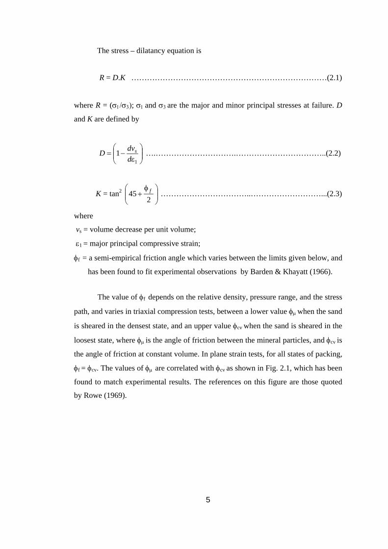
The stress – dilatancy equation is
R = D.K …………………………………………………………………(2.1)
where R = (σ1/σ3); σ1 and σ3
are the major and minor principal stresses at failure. D
and K are defined by
⎟⎟⎠
⎞⎜⎜⎝
⎛ε
−=1
1ddvD s ….………………………….……………………………..(2.2)
K = tan2 ⎟⎟⎠
⎞⎜⎜⎝
⎛ φ+
245 f ……………………………..………………………...(2.3)
where
vs = volume decrease per unit volume;
ε1 = major principal compressive strain;
φf = a semi-empirical friction angle which varies between the limits given below, and
has been found to fit experimental observations by Barden & Khayatt (1966).
The value of φf depends on the relative density, pressure range, and the stress
path, and varies in triaxial compression tests, between a lower value φµ when the sand
is sheared in the densest state, and an upper value φcv when the sand is sheared in the
loosest state, where φµ is the angle of friction between the mineral particles, and φcv is
the angle of friction at constant volume. In plane strain tests, for all states of packing,
φf = φcv. The values of φµ are correlated with φcv as shown in Fig. 2.1, which has been
found to match experimental results. The references on this figure are those quoted
by Rowe (1969).
5
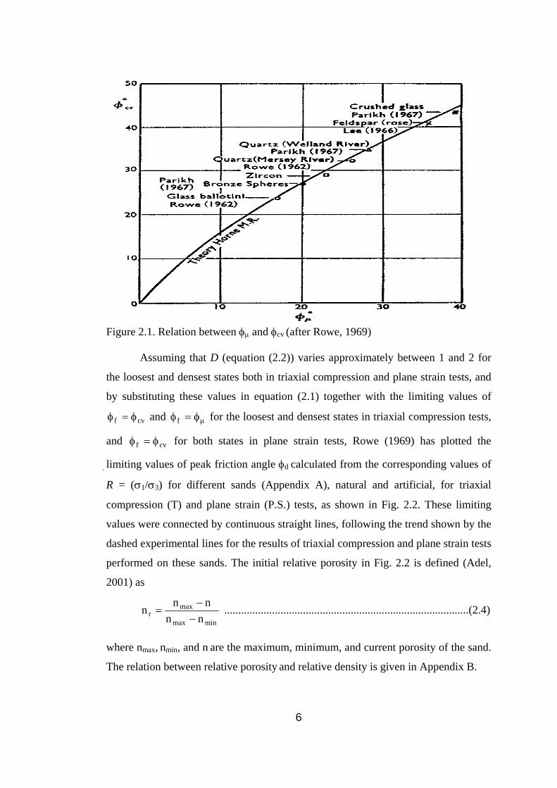
Figure 2.1. Relation between φµ and φcv (after Rowe, 1969) Assuming that D (equation (2.2)) varies approximately between 1 and 2 for
the loosest and densest states both in triaxial compression and plane strain tests, and
by substituting these values in equation (2.1) together with the limiting values of
and cvf φ=φ µφ=φf for the loosest and densest states in triaxial compression tests,
and for both states in plane strain tests, Rowe (1969) has plotted the cvf φ=φ
limiting values of peak friction angle φd calculated from the corresponding values of
R = (σ1/σ3) for different sands (Appendix A), natural and artificial, for triaxial
compression (T) and plane strain (P.S.) tests, as shown in Fig. 2.2. These limiting
values were connected by continuous straight lines, following the trend shown by the
dashed experimental lines for the results of triaxial compression and plane strain tests
performed on these sands. The initial relative porosity in Fig. 2.2 is defined (Adel,
2001) as
minmax
maxr nn
nnn
−−
= .......................................................................................(2.4)
where nmax, nmin, and n are the maximum, minimum, and current porosity of the sand.
The relation between relative porosity and relative density is given in Appendix B.
6
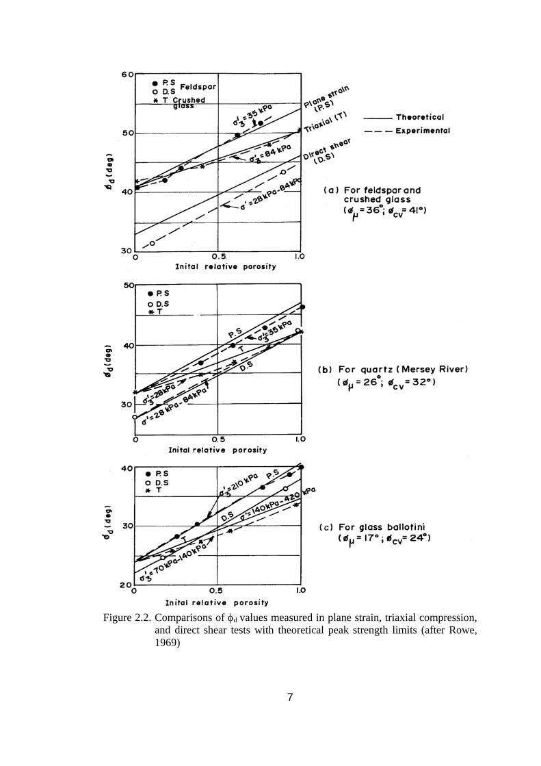
Figure 2.2. Comparisons of φd values measured in plane strain, triaxial compression, and direct shear tests with theoretical peak strength limits (after Rowe, 1969)
7

Rowe (1969) also derived the following relation between the peak friction
angles measured in direct simple shear φds and plane strain φps for all states of
packing.
cvpsds costantan φφ=φ …………………………….…………………(2.5)
Experimental results presented show that the conventional shear box test
results are also closely consistent with equation (2.5). Rowe (1969) used equation
(2.5) and the results of conventional shear box tests to plot the curves shown in
Fig. 2.2 for the direct shear (D.S.) test.
The relations in Fig. 2.2 allow overall comparison of φd values in the three
types of test when the effects of the orientation of the shear plane and of the
confining pressure and so the crushing of sand particles on the measured φd values
were disregarded. These effects are discussed in subsequent sub-sections.
2.1.2 Effect of Initial Void Ratio
Void ratio is perhaps the most important single parameter that affects the
strength of sands (Mitchell, 1976; Maeda & Miura, 1999(a)). Generally, for drained
tests either in triaxial or direct shear tests, the lower the void ratio, the higher the
shear strength. The effect of void ratio on the friction angle (φd ) can be explained by
the phenomenon of interlocking (Lambe & Whitman, 1979). The denser the sand, the
greater the interlocking, and so the greater the value of φd.
Bardet (1997) gives possible ranges of the peak friction angle φd and the
friction angle φcv at constant volume at different densities for different frictional soils
(Table 2.1), which is in conformity with Lambe & Whitman’s (1979) views that the
lower the void ratio, the higher the shear strength.
8
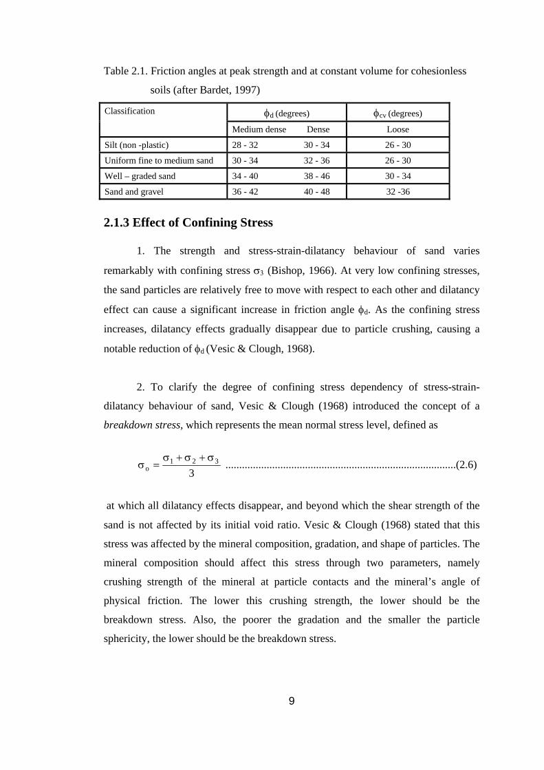
Table 2.1. Friction angles at peak strength and at constant volume for cohesionless
soils (after Bardet, 1997)
φd (degrees) φcv (degrees) Classification
Medium dense Dense Loose
Silt (non -plastic) 28 - 32 30 - 34 26 - 30
Uniform fine to medium sand 30 - 34 32 - 36 26 - 30
Well – graded sand 34 - 40 38 - 46 30 - 34
Sand and gravel 36 - 42 40 - 48 32 -36
2.1.3 Effect of Confining Stress
1. The strength and stress-strain-dilatancy behaviour of sand varies
remarkably with confining stress σ3 (Bishop, 1966). At very low confining stresses,
the sand particles are relatively free to move with respect to each other and dilatancy
effect can cause a significant increase in friction angle φd. As the confining stress
increases, dilatancy effects gradually disappear due to particle crushing, causing a
notable reduction of φd (Vesic & Clough, 1968).
2. To clarify the degree of confining stress dependency of stress-strain-
dilatancy behaviour of sand, Vesic & Clough (1968) introduced the concept of a
breakdown stress, which represents the mean normal stress level, defined as
3321
oσ+σ+σ
=σ ....................................................................................(2.6)
at which all dilatancy effects disappear, and beyond which the shear strength of the
sand is not affected by its initial void ratio. Vesic & Clough (1968) stated that this
stress was affected by the mineral composition, gradation, and shape of particles. The
mineral composition should affect this stress through two parameters, namely
crushing strength of the mineral at particle contacts and the mineral’s angle of
physical friction. The lower this crushing strength, the lower should be the
breakdown stress. Also, the poorer the gradation and the smaller the particle
sphericity, the lower should be the breakdown stress.
9
3. The stress-strain-dilatancy behaviour of sands under various σ3 values was
investigated by a number of researchers. A summary of each follows.
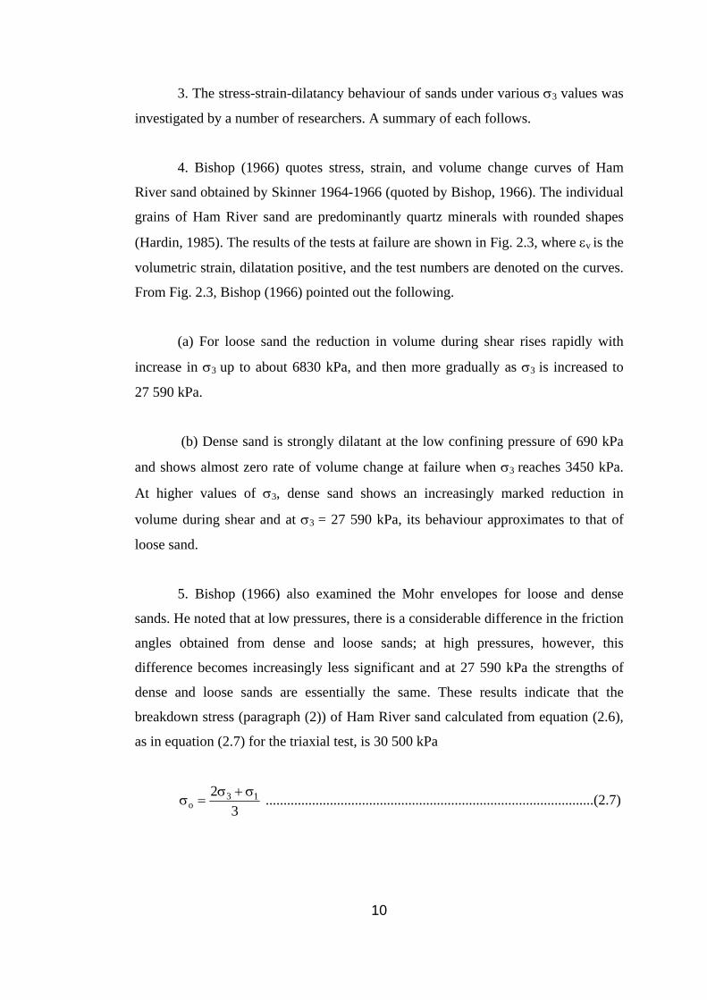
4. Bishop (1966) quotes stress, strain, and volume change curves of Ham
River sand obtained by Skinner 1964-1966 (quoted by Bishop, 1966). The individual
grains of Ham River sand are predominantly quartz minerals with rounded shapes
(Hardin, 1985). The results of the tests at failure are shown in Fig. 2.3, where εv is the
volumetric strain, dilatation positive, and the test numbers are denoted on the curves.
From Fig. 2.3, Bishop (1966) pointed out the following.
(a) For loose sand the reduction in volume during shear rises rapidly with
increase in σ3 up to about 6830 kPa, and then more gradually as σ3 is increased to
27 590 kPa.
(b) Dense sand is strongly dilatant at the low confining pressure of 690 kPa
and shows almost zero rate of volume change at failure when σ3 reaches 3450 kPa.
At higher values of σ3, dense sand shows an increasingly marked reduction in
volume during shear and at σ3 = 27 590 kPa, its behaviour approximates to that of
loose sand.
5. Bishop (1966) also examined the Mohr envelopes for loose and dense
sands. He noted that at low pressures, there is a considerable difference in the friction
angles obtained from dense and loose sands; at high pressures, however, this
difference becomes increasingly less significant and at 27 590 kPa the strengths of
dense and loose sands are essentially the same. These results indicate that the
breakdown stress (paragraph (2)) of Ham River sand calculated from equation (2.6),
as in equation (2.7) for the triaxial test, is 30 500 kPa
32 13
oσ+σ
=σ ............................................................................................(2.7)
10

20 29
6
5
2020
LOOSE
σ3 = 27 590 kPa
70 000
14 000
28 000
42 000
56 000
ε v
(%)
0
σ3 = 6830 kPa29
σ3 = 3450 kPa
σ3 = 690 kPa 5
6
(σ
1-σ 3
) (kP
a)
Str
ess
diffe
renc
e (σ
1-σ 3
) (kP
a)
14 000
28 000
42 000
56 000
27
26
25
21
0
DENSE
σ3 = 27 590 kPa21
LIMIT OF TEST
σ3 = 3450 kPa 25
26
27 σ3 = 690 kPa
σ3 = 6830 kPa
+5 0
-15
-5 -10
ε v
(%)
0 10 20 30 40 50 0 10 20 30 40 50
Axial strain ε1 (%) ε1 (%)
0 -5 -10 -15 -20
70 000
Figure 2.3. Results of drained tests on Ham River sand (after Bishop, 1966)
6. Seed & Lee (1967) investigated the drained strength characteristics of
sands over a wide range of confining pressures. The soil used for this investigation
was fine uniform sand that had been dredged from the Sacramento River. The
individual grains were mostly feldspar and quartz minerals with subangular to
subrounded shapes. Seed & Lee (1967) examined the relationships between stress,
strain, and volume change in a series of drained triaxial tests on dense sand under
increasing confining pressures, and observed that an increase in σ3 increased the
11

strain to failure, and decreased the tendency to dilate. Similar results were obtained
from a series of drained triaxial tests on loose sand. The pattern is similar to that for
dense sand, except that at low pressures the tendency for dilation is not so strong as
for dense sand. Seed & Lee (1967) also found that the local slope of the Mohr
envelope for dense sand at low confining stresses σ3, below 800 kPa, was about 41o,
but at the higher values of σ3, up to 4000 kPa, it reduced to about 24o. A similar trend
was observed for the loose sand, the corresponding reduction being from 34o to 24o.
These results indicate that the breakdown stress (paragraph (2)) of Sacramento River
sand, calculated from equation (2.7) is 7000 kPa.
7. Vesic & Clough (1968) performed triaxial tests on Chattahoochee sand to
investigate the effect of σ3 on the behaviour of cohesionless soils. The individual
grains of Chattahoochee sand were predominantly quartz and some mica minerals
with subangular shapes (Hardin, 1985). Under the mean normal stresses σo (equation
(2.6)) below 100 kPa, there was very little crushing, and dilatancy effects were quite
significant. At higher σo, up to 10 000 kPa, crushing became more pronounced, and
dilatancy effects gradually disappeared. At σo = 10 000 kPa, dilatancy effects
completely disappeared, indicating that the breakdown stress (paragraph (2)) of
Chattahoochee sand is 10 000 kPa.
8. Breakdown stresses of Ham River sand, Chattahoochee sand, and
Sacramento River sand were found as 30 500 kPa, 10 000 kPa, and 7000 kPa by
Skinner (1964-1966) (quoted by Bishop, 1966), Vesic & Clough (1968), and Seed &
Lee (1967) respectively (paragraphs (5) to (7)). It is seen that (i) Ham River sand of
predominantly quartz minerals with rounded shapes has the highest breakdown
stress; (ii) Chattahoochee sand of predominantly quartz and some mica minerals with
subangular shapes has the intermediate breakdown stress; (iii) Sacramento River
sand of mostly feldspar, the grains of which have lower resistance to crushing
compared to quartz grains (Norman, 2000(b)), and quartz minerals with subangular
to subrounded shapes has the lowest breakdown stress. This is a confirmation of the
views, quoted in paragraph (2), that mineral composition and shape of sand particles
12
affect breakdown stress, and that for sands with grains of low strength and angular
shape, breakdown stress is lower.
9. Maeda & Miura (1999(b)) studied the deformation – failure behaviour of
some 80 granular materials in a series of triaxial tests at σ3 values between 50 kPa
and 400 kPa. The peak angle of friction φd was found to decrease with an increase in
σ3, as observed by Bishop (1966), Seed & Lee (1967), and Vesic & Clough (1968)
(paragraphs (5) to (7) respectively). Maeda & Miura (1999(b)) stated that the higher
reduction in the values of φd was observed on granular materials which possess a
high value of angularity and void ratio extent (difference between maximum void
ratio, emax, and minimum void ratio, emin). Void ratio extent is controlled mainly by
the gradation, shape, and size of the sand particles (Youd, 1973; Shahu & Yudhbir,
1998; Maeda & Miura, 1999(a)). For specimens consisting of uniformly graded,
rounded particles (e.g., Leighton Buzzard sand and glass beads), the value of
(emax – emin) is roughly one half of the corresponding value for specimens consisting
of well graded, angular particles (e.g., Kalpi sand and Biddulph sand) for any given
value of average particle size (Yudhbir et al., 1991) (quoted by Shahu & Yudhbir,
1998).
10. From paragraphs (5), (6), (7), and (9), the reduction in φd of sands,
observed with an increase in σ3, seems to be linked with the gradation, shape, and the
mineralogical composition of the sand particles.
2.1.4 Effect of Intermediate Principal Stress
1. The effect of intermediate principal stress σ2 is seen in the results of
triaxial and plane strain tests. The triaxial test simulates an axisymmetric condition
(three-dimensional strain), and the plane strain test simulates a two-dimensional
loading condition (two-dimensional strain). Denoting the major, intermediate, and
minor principal stresses σ1, σ2, and σ3, respectively, and the corresponding principal
strains by ε1, ε2, and ε3, the stress - strain conditions are given as follows:
13

For the plane strain test,
σ1 > σ2 > σ3 ε1≠0 ε2=0 ε3≠0
For the triaxial compression test,
σ1 > σ2 = σ3 ε1≠0 ε2=ε3≠0
2. Shear strength of sands measured in plane strain tests is greater than that
measured in triaxial tests (Leussink & Whitke, 1963; Lee, 1970; Cornforth, 1973;
Schanz & Vermeer, 1996). The reason for the increased resistance in the plane strain
tests comes about because the sand particles are given less freedom in the way that
they can move around adjacent particles so as to overcome interlocking (Mitchell,
1976).
3. A number of researchers investigated the variation of the difference
between the peak friction angles measured in plane strain tests (φps) and triaxial tests
(φt) with density and confining pressure. A summary of each follows.
4. Leussink & Whitke (1963) performed plane strain and triaxial tests on
glass balls with a constant diameter of approximately 15 mm at confining pressures
σ3 of between 50 kPa and 300 kPa. They obtained φps = 51.4o and φt = 40.7o,
indicating a difference of about 11o between the peak friction angles.
5. Lee (1970) performed plane strain and triaxial tests on specimens of
Sacramento River sand prepared at two different initial relative densities Dr of 38%
and 78% at σ3 values of 30 kPa to 1000 kPa. The difference (φps - φt) was 8o for
dense specimens at σ3 values lower than 100 kPa, and vanished both for loose
specimens at all σ3 values and for dense specimens at sufficiently high σ3 values to
prevent dilation. These results indicate that (φps - φt) is linked with dilatation and so
with σ3 and density.
14
6. Cornforth (1973) performed plane strain and triaxial tests on specimens of
Brasted sand prepared at initial Dr values ranging from 15% to 80% at σ3 = 280 kPa.
The results of these tests indicated the following. The values of φps were higher than
those of φt. A decrease in Dr caused the difference (φps - φt) to decrease. The
difference was about 4o to 5o for dense specimens and decreased to about 1o for loose
specimens. The ultimate strength of the sand at all densities was approximately
constant and nearly the same in both plane strain and triaxial tests. These results
indicate that, in contrast to the peak strength, the ultimate strength of sand is
independent of strain conditions and void ratio.
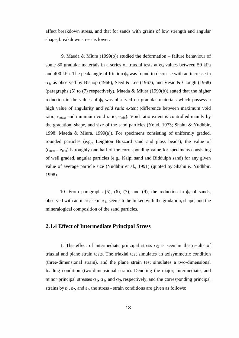
7. Similar results were obtained by Hussaini (1973) who performed plane
strain and triaxial tests on specimens of Chattahoochee sand prepared at initial Dr
between 30 % and 100 %, at σ3 = 490 kPa. The results of these tests are shown in
Fig. 2.4, from which the following can be noted.
Triaxial compression
Plane strain
σ3 = 490 kPa
P
eak
angl
e of
fric
tion
φ d (d
egre
es)
Initial relative density Dr (%)
Figure 2.4. Variation of the peak angle of friction with initial relative density for
Chattahoochee sand (after Hussaini, 1973)
15
(a) An increase in Dr resulted in an increase in both φps and φt.
(b) The values of φps were higher than those of φt. A decrease in Dr caused
the difference (φps - φt) to decrease, as observed by Lee (1970) and Cornforth (1973)
(paragraphs (5) and (6)); the difference was about 3o for dense sand and about 1o for
loose sand.
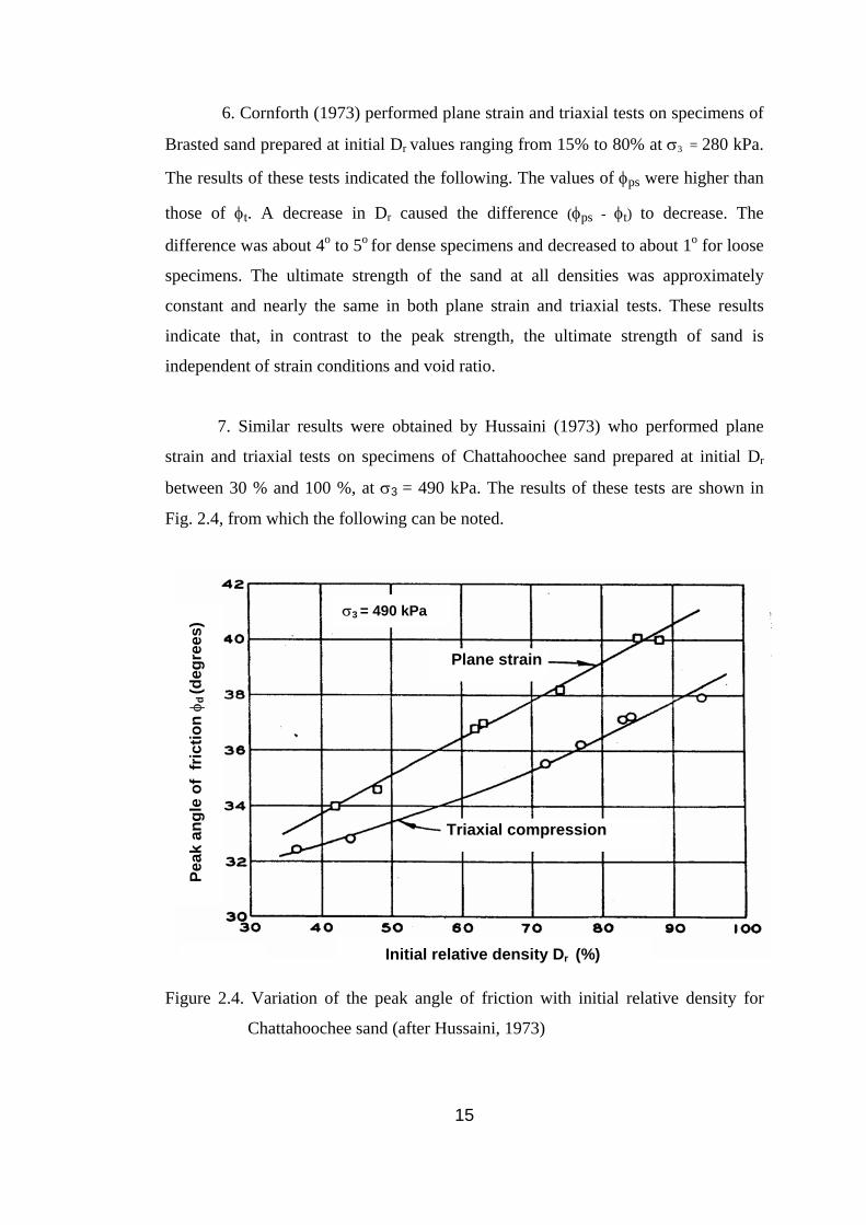
8. Marachi et al. (1981) performed plane strain and triaxial tests on specimens
of Monterey sand prepared at densities ranging from loose to dense, under
σ3 = 70 kPa to 3450 kPa. Specimens were prepared to initial void ratios eo of 0.75,
0.65, and 0.55, corresponding to initial Dr of 27 %, 60 %, and 90 % respectively.
Typical stress - strain curves for plane strain and triaxial tests at σ3 = 70 kPa are
shown in Fig. 2.5, from which the following can be noted.
Loose eo = 0.75
Medium dense eo = 0.65 Dense
eo = 0.55
Prin
cipa
l str
ess
ratio
(σ1/σ
3)
Axial strain (%)
Figure 2.5. Stress - strain relationship for plane strain and triaxial specimen
(σ3 = 70 kPa) (after Marachi et al., 1981)
(a) The plane strain test yields higher values of maximum principal stress
ratio (σ1/σ3)f than the triaxial test for the same void ratio.
16
(b) An increase in eo causes a decrease in (σ1/σ3)f for both triaxial and plane
strain tests.
(c) When eo increases, the difference between the (σ1/σ3)f values for plane
strain and triaxial tests decreases.
(d) The plane strain specimens fail or reach (σ1/σ3)f value at smaller values
of axial strain (ε1)f than the triaxial specimens.
(e) The values of (ε1)f for plane strain and triaxial tests are larger for loose
specimens than for dense specimens.
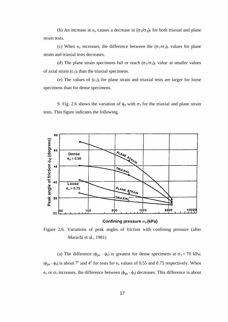
9. Fig. 2.6 shows the variation of φd with σ3 for the triaxial and plane strain
tests. This figure indicates the following.
Figure 2.6. Variations of peak angles of friction with confining pressure (after
Marachi et al., 1981)
e Loose
o = 0.75
Dense eo = 0.55
P
eak
angl
e of
fric
tion
φ d (d
egre
es)
Confining pressure σ3 (kPa)
(a) The difference (φps - φt) is greatest for dense specimens at σ3 = 70 kPa;
(φps - φt) is about 7o and 4o for tests for eo values of 0.55 and 0.75 respectively. When
eo or σ3 increases, the difference between (φps - φt) decreases. This difference is about
17
1o for σ3 = 3450 kPa. These results confirm Lee’s (1970) findings (paragraph (5))
that the difference between values of φps and φt is linked with dilatation.
(b) The φd values are found to be higher for dense sands than for loose sands,
which is due to greater interlocking in the former in conformity with Lambe &
Whitman’s (1979) views (section 2.1.2). For both dense and loose specimens, an
increase in σ3 causes a decrease in φd measured in both tests, which is due to particle
crushing, as discussed in section 2.1.3.
10. By considering Matsuoka’s (1974) (quoted by Wroth, 1984) failure
criterion for soils, Wroth (1984) investigated the effect of intermediate principal
stress on shear strength. He gives the following approximate relation.
8 (φps) = 9 (φt) ……………………...………………………….....(2.8)
11. This equation does not take into account factors which influence shear
strength of sands such as density, confining stress, mineralogical composition,
inclination of the shear plane to the bedding planes.
12. Bolton (1986) collated extensive data on the strength and dilatancy of 17
sands available in the literature in plane strain and triaxial tests at different densities
and confining pressures to produce empirical relations by which φd could be
predicted. He introduced a relative dilatancy index (IR), in terms of relative density
and applied stress level, of the form
IR = Dr [Qg – ln(p')] – s ………………………………………..………….(2.9)
where p' (kPa) is the mean effective stress (σ1′+σ3
′) / 2 ; Qg is a function of grain
type, and s is a constant.
18
13. In deriving simple correlations amongst IR, Dr, and p', it was found that
Qg = 10 and s = 1 gave the best fit for the different sands collated. This yielded
IR = Dr [10 – ln(p')] – 1 ……..........……………………………………(2.10)
14. Bolton (1986) also obtained the following correlations between IR and
(φd - φcv):
For plane strain tests
(φps) - (φcv)ps ≈ 5 IR ……………………………………...............(2.11)
For triaxial tests
(φt) - (φcv)t ≈ 3 IR ……………………………………...................(2.12)
where (φcv)ps and (φcv)t are the ultimate friction angles measured in plane strain and
triaxial tests respectively.
15. Bolton (1986) stated that the sands presented in his study were mainly of
quartz and feldspar (Qg = 10); the presence of substantial proportions of mica, calcite
or other materials (Qg ≈ 5 to 8) would be bound to affect both φcv and the crushing
which reduces IR at high stresses; this implies that the parameter Qg in equation (2.9)
should be reduced for soils of weaker grains.
16. Schanz & Vermeer (1996) have eliminated IR between equations (2.11)
and (2.12), and obtained the following equation to correlate φps and φt for sands.
φt = ( 3 φps+ 2 φcv) / 5 ……………......…………………………….(2.13)
19
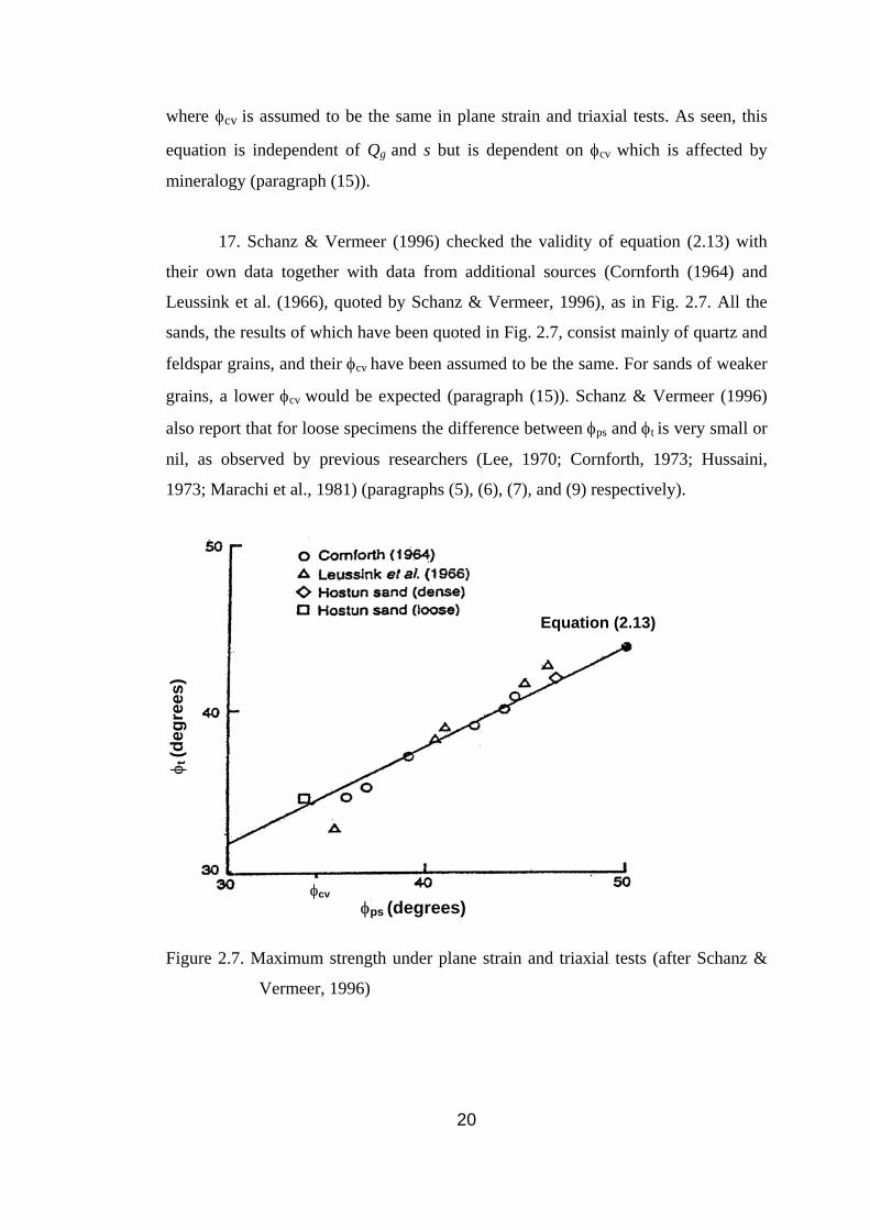
where φcv is assumed to be the same in plane strain and triaxial tests. As seen, this
equation is independent of Qg and s but is dependent on φcv which is affected by
mineralogy (paragraph (15)).
17. Schanz & Vermeer (1996) checked the validity of equation (2.13) with
their own data together with data from additional sources (Cornforth (1964) and
Leussink et al. (1966), quoted by Schanz & Vermeer, 1996), as in Fig. 2.7. All the
sands, the results of which have been quoted in Fig. 2.7, consist mainly of quartz and
feldspar grains, and their φcv have been assumed to be the same. For sands of weaker
grains, a lower φcv would be expected (paragraph (15)). Schanz & Vermeer (1996)
also report that for loose specimens the difference between φps and φt is very small or
nil, as observed by previous researchers (Lee, 1970; Cornforth, 1973; Hussaini,
1973; Marachi et al., 1981) (paragraphs (5), (6), (7), and (9) respectively).
φps (degrees)
φcv
φ
t (de
gree
s)
Equation (2.13)
Figure 2.7. Maximum strength under plane strain and triaxial tests (after Schanz &
Vermeer, 1996)
20

18. Mirata & Gökalp (1997) tested the applicability of the cylindrical wedge
shear test (cylwest) (Mirata, 1991) to sands. A sand to which 30% crushed stone of
up to 10 mm particles was added (sample S1), and the same sand with 30%
subangular gravel up to 5 mm particles (sample S2) were tested in cylwests and
triaxial tests. They investigated the difference between φps and φt by assuming that
φd values measured in cylwests represent φps; their results are given in Fig. 2.8
against φt. The circular point represents the results of the tests on sample S1, and the
triangular point those on sample S2. The chain-dotted lines representing equation
(2.13) for these samples have been plotted by assuming φcv to be equal to the
ultimate friction angle measured in cylwests. The full line represents equation (2.13)
for the Hostun sand tested by Schanz & Vermeer (1996). The dashed line represents
Wroth’s (1984) equation (2.8). For a given φcv, the proximity of the results to both
Wroth (1984) : φps = 89 φt
φ
t (de
gree
s)
φps (degrees)
: Test results for S2
: Test results for S1
2 : Eq. (2.13) for sample S2
1 : Eq. (2.13) for sample S1
H : Eq. (2.13) for Hostun sand
Figure 2.8. Comparison of relationships between peak angles of friction in plane
strain and triaxial tests (after Mirata & Gökalp, 1997)
21

Schanz & Vermeer’s (1996) equation (2.13) and to Wroth’s (1984) equation (2.8),
particularly for sample S2, was found noteworthy by Mirata & Gökalp (1997), who
suggested that in the absence of plane strain equipment, the cylwest might be used to
investigate the difference between φps and φt.
19. Adel (2001) performed triaxial and plane strain tests on samples of three
types of silica sand at σ3 values of 172 kPa and 344 kPa. The physical properties of
the sands are summarized in Table 2.2. He obtained results indicating the following.
Table 2.2. Physical properties of the sands (after Adel, 2001)
Sand type Grading Particle shape
Gs emax
emin
Cu D50
A Uniform Rounded 2.65 0.80 0.40 2.40 0.22
B Uniform Angular 2.63 0.90 0.50 2.33 0.65
C Well graded Angular 2.64 0.95 0.40 2.00 0.65
(a) The values of φps were about 5% to 12% higher than those of φt for dense
sands, whereas they were slightly higher or equal for the case of loose sands. This is
consistent with previous findings (Lee, 1970; Cornforth, 1973; Hussaini, 1973;
Marachi et al., 1981; Schanz & Vermeer, 1996) (paragraphs (5), (6), (7), (9), and
(17) respectively).
(b) The values of axial strain at failure (ε)f for triaxial tests were always
higher than those for plane strain tests for the same initial porosity. This is in
conformity with Fig. 2.5.
(c) The values of volumetric strain (εv) were higher for dense sand than for
loose sand. The values of εv at failure (εv)f for sand C were higher than those for
sands A and B under the same conditions. This was due to the fact that sand C was
well graded with angular particles, which resulted in a high degree of interlocking
between particles, and so to a larger dilatation during shear.
22

2.1.5 Effect of Particle Composition
2.1.5.1 Definitions
“The use of relative density correlations based on an average sand to predict
soil behaviour without considering the particle composition can result in poor or
misleading predictions. So, this question arises: Do granular soils at the same relative
density have the same properties? Tests on medium to fine sands with varying
particle compositions indicate that granular soils at the same relative density can
have drastically different engineering properties. Variations in engineering properties
due to particle composition can be as large as variations associated with large
differences in relative densities.” (Holubec & D’Appolonia, 1973.)
The composition of sand can have an important influence on its friction
angle, indirectly by influencing initial void ratio eo, and directly by influencing the
amount of interlocking occurring for a given eo (Kezdi, 1974).
Composition effect can be explained in terms of the size, shape, gradation,
and mineralogy of the particles. The particle size effect on the shear strength can be
evaluated by varying the effective size, D10, of the particles. The gradation effect on
the shear strength can be evaluated by varying the coefficient of uniformity (Cu) of
the soil. The particle shape effect can be evaluated by varying sphericity and
angularity. (Koerner, 1970.) The definitions and method of measurement of some of
these properties are given in the following paragraphs.
The following paragraph has been summarized from Yudhbir & Rahim
(1991); the references are those quoted by the authors.
Sedimentologists generally express particle shape in terms of surface texture,
sphericity, and roundness (Blatt et al., 1971). Surface texture is used to describe
irregularities of the surface of particles that are too small to affect the overall shape.
23
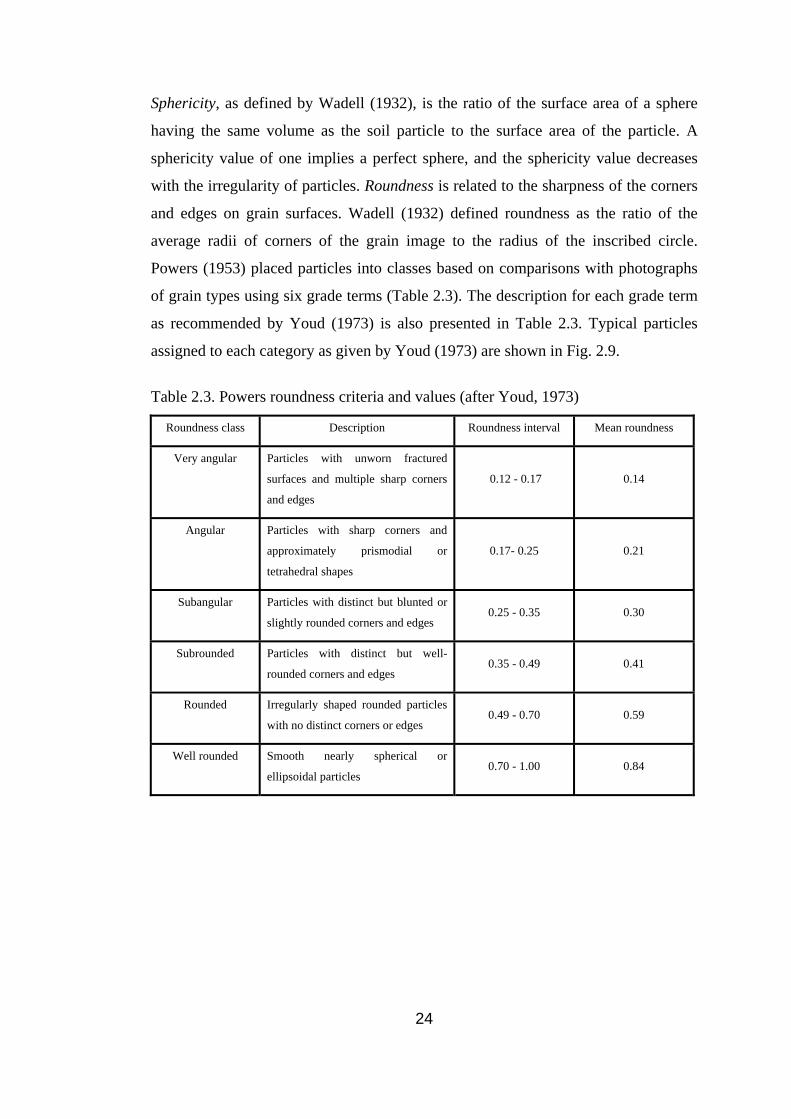
Sphericity, as defined by Wadell (1932), is the ratio of the surface area of a sphere
having the same volume as the soil particle to the surface area of the particle. A
sphericity value of one implies a perfect sphere, and the sphericity value decreases
with the irregularity of particles. Roundness is related to the sharpness of the corners
and edges on grain surfaces. Wadell (1932) defined roundness as the ratio of the
average radii of corners of the grain image to the radius of the inscribed circle.
Powers (1953) placed particles into classes based on comparisons with photographs
of grain types using six grade terms (Table 2.3). The description for each grade term
as recommended by Youd (1973) is also presented in Table 2.3. Typical particles
assigned to each category as given by Youd (1973) are shown in Fig. 2.9.
Table 2.3. Powers roundness criteria and values (after Youd, 1973)
Roundness class Description Roundness interval Mean roundness
Very angular Particles with unworn fractured
surfaces and multiple sharp corners
and edges
0.12 - 0.17 0.14
Angular Particles with sharp corners and
approximately prismodial or
tetrahedral shapes
0.17- 0.25 0.21
Subangular Particles with distinct but blunted or
slightly rounded corners and edges 0.25 - 0.35 0.30
Subrounded Particles with distinct but well-
rounded corners and edges 0.35 - 0.49 0.41
Rounded Irregularly shaped rounded particles
with no distinct corners or edges 0.49 - 0.70 0.59
Well rounded Smooth nearly spherical or
ellipsoidal particles 0.70 - 1.00 0.84
24
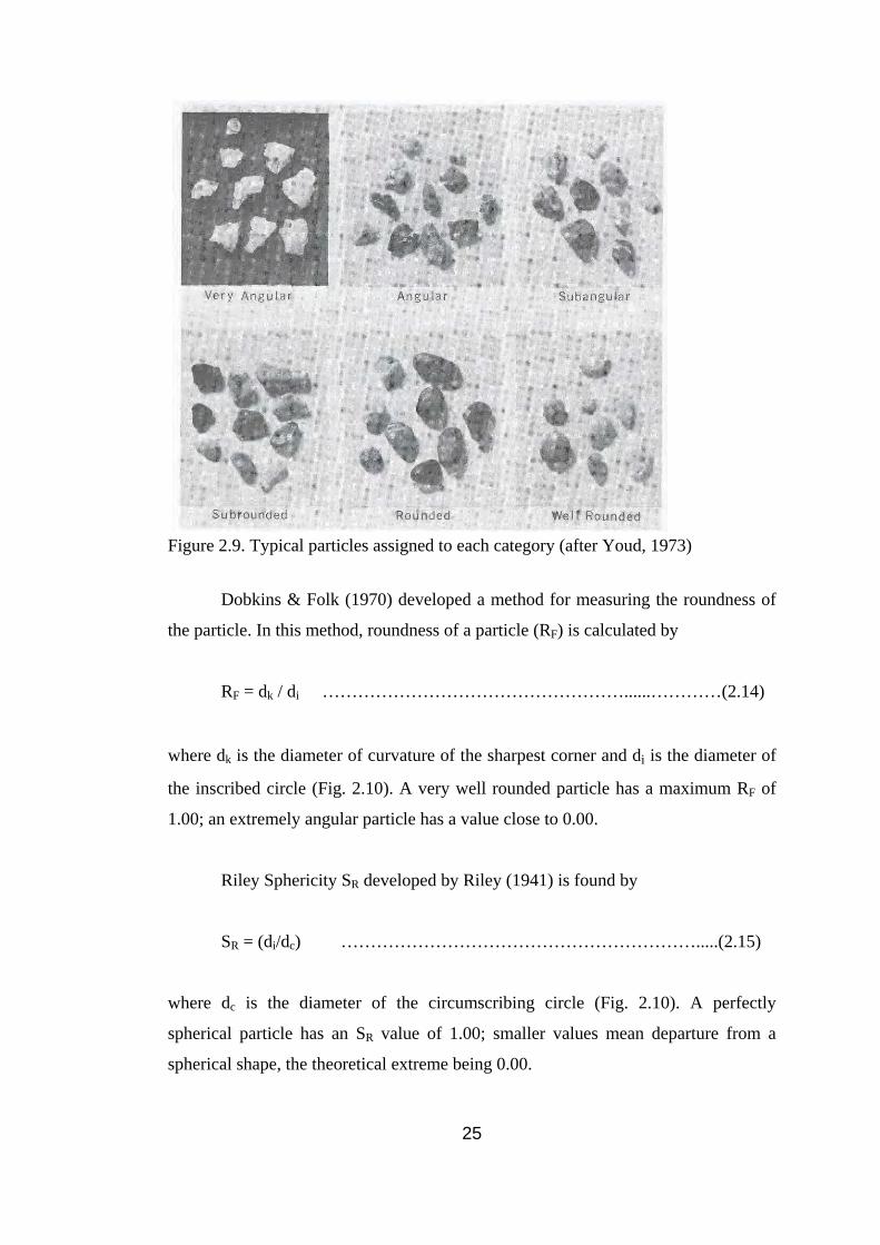
Figure 2.9. Typical particles assigned to each category (after Youd, 1973)
Dobkins & Folk (1970) developed a method for measuring the roundness of
the particle. In this method, roundness of a particle (RF) is calculated by
RF = dk / di ……………………………………………......…………(2.14)
where dk is the diameter of curvature of the sharpest corner and di is the diameter of
the inscribed circle (Fig. 2.10). A very well rounded particle has a maximum RF of
1.00; an extremely angular particle has a value close to 0.00.
Riley Sphericity SR developed by Riley (1941) is found by
SR = (di/dc) …………………………………………………….....(2.15)
where dc is the diameter of the circumscribing circle (Fig. 2.10). A perfectly
spherical particle has an SR value of 1.00; smaller values mean departure from a
spherical shape, the theoretical extreme being 0.00.
25
dc
O
di
dk
Figure 2.10. Definitions of angularity and sphericity (after Norman, 2000(c))
The calculations of sphericity and roundness are complex; but the values of
RF and SR can be estimated by using comparison charts (Fig. 2.11) including
silhouettes or photographs of grains whose roundness and sphericity values have
already been calculated.
2.1.5.2 Effect of Particle Shape and Mineral Composition
The following paragraph has been taken from Shahu & Yudhbir (1998); the
references are those quoted by the authors.
The angularity and mineralogical composition of a sand affect its mechanical
and engineering properties significantly. Winterkorn & Fang (1986) have stated that
the peak angle of friction φd value for a given initial relative density Dr depends
largely upon particle shape and gradation of sand. Rahim (1989) has shown that the
mechanical characteristics of a sand such as its compressibility and crushing are
strongly influenced by the shape of sand particles (Yudhbir & Wood 1989; Yudhbir
& Rahim, 1991).
26

Degrees of roundness according to Russel-Taylor-Pettijohn (after Schneiderhöhn, 1954) (quoted by Norman, 2000(c)). From top to bottom: angular - subangular - subrounded - rounded - well rounded.
Figure 2.11. A visual comparison chart for roundness and sphericity (after Norman,
2000(c))
27
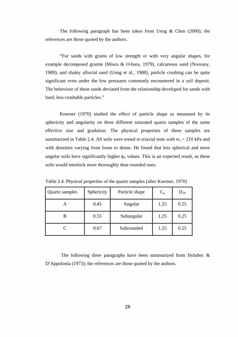
The following paragraph has been taken from Ueng & Chen (2000); the
references are those quoted by the authors.
“For sands with grains of low strength or with very angular shapes, for
example decomposed granite (Miura & O-hara, 1979), calcareous sand (Noorany,
1989), and shaley alluvial sand (Ueng et al., 1988), particle crushing can be quite
significant even under the low pressures commonly encountered in a soil deposit.
The behaviour of these sands deviated from the relationship developed for sands with
hard, less crushable particles.”
Koerner (1970) studied the effect of particle shape as measured by its
sphericity and angularity on three different saturated quartz samples of the same
effective size and gradation. The physical properties of these samples are
summarized in Table 2.4. All soils were tested in triaxial tests with σ3 = 210 kPa and
with densities varying from loose to dense. He found that less spherical and more
angular soils have significantly higher φd values. This is an expected result, as these
soils would interlock more thoroughly than rounded ones.
Table 2.4. Physical properties of the quartz samples (after Koerner, 1970)
Quartz samples Sphericity Particle shape Cu D10
A 0.45 Angular 1.25 0.25
B 0.55 Subangular 1.25 0.25
C 0.67 Subrounded 1.25 0.25
The following three paragraphs have been summarized from Holubec &
D’Appolonia (1973); the references are those quoted by the authors.
28
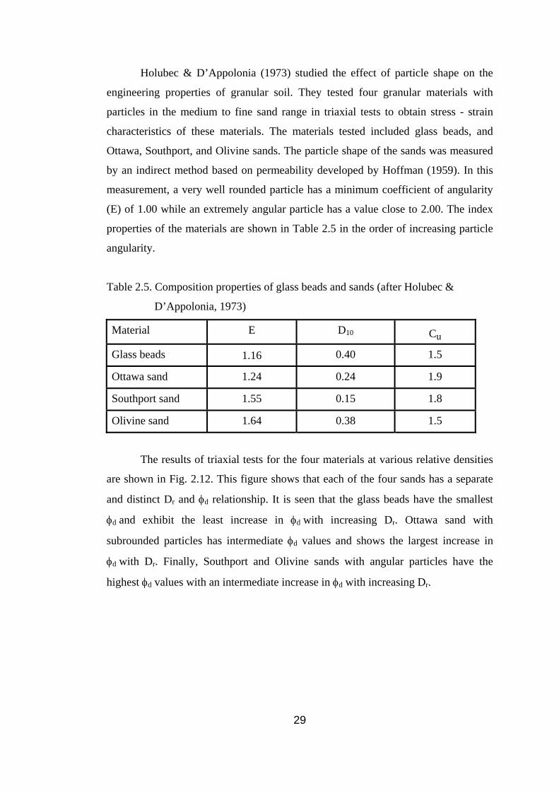
Holubec & D’Appolonia (1973) studied the effect of particle shape on the
engineering properties of granular soil. They tested four granular materials with
particles in the medium to fine sand range in triaxial tests to obtain stress - strain
characteristics of these materials. The materials tested included glass beads, and
Ottawa, Southport, and Olivine sands. The particle shape of the sands was measured
by an indirect method based on permeability developed by Hoffman (1959). In this
measurement, a very well rounded particle has a minimum coefficient of angularity
(E) of 1.00 while an extremely angular particle has a value close to 2.00. The index
properties of the materials are shown in Table 2.5 in the order of increasing particle
angularity.
Table 2.5. Composition properties of glass beads and sands (after Holubec &
D’Appolonia, 1973)
Material E D10 Cu
Glass beads 1.16 0.40 1.5
Ottawa sand 1.24 0.24 1.9
Southport sand 1.55 0.15 1.8
Olivine sand 1.64 0.38 1.5
The results of triaxial tests for the four materials at various relative densities
are shown in Fig. 2.12. This figure shows that each of the four sands has a separate
and distinct Dr and φd relationship. It is seen that the glass beads have the smallest
φd and exhibit the least increase in φd with increasing Dr. Ottawa sand with
subrounded particles has intermediate φd values and shows the largest increase in
φd with Dr. Finally, Southport and Olivine sands with angular particles have the
highest φd values with an intermediate increase in φd with increasing Dr.
29
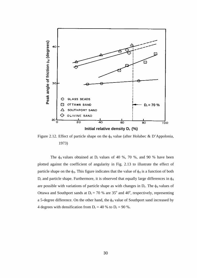
Dr = 70 %
Initial relative density Dr (%)
Pea
k an
gle
of fr
ictio
n φ d
(deg
rees
)
Figure 2.12. Effect of particle shape on the φd value (after Holubec & D’Appolonia,
1973)
The φd values obtained at Dr values of 40 %, 70 %, and 90 % have been
plotted against the coefficient of angularity in Fig. 2.13 to illustrate the effect of
particle shape on the φd. This figure indicates that the value of φd is a function of both
Dr and particle shape. Furthermore, it is observed that equally large differences in φd
are possible with variations of particle shape as with changes in Dr. The φd values of
Ottawa and Southport sands at Dr = 70 % are 35o and 40o, respectively, representing
a 5-degree difference. On the other hand, the φd value of Southport sand increased by
4 degrees with densification from Dr = 40 % to Dr = 90 %.
30
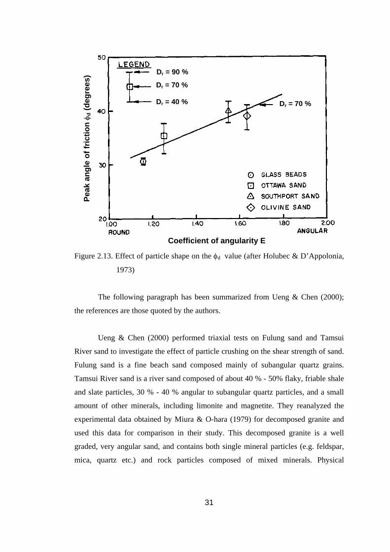
Pea
k an
gle
of fr
ictio
n φ d
(deg
rees
)
Coefficient of angularity E
Dr = 40 %
Dr = 70 %
Dr = 90 %
Dr = 70 %
Figure 2.13. Effect of particle shape on the φd value (after Holubec & D’Appolonia,
1973)
The following paragraph has been summarized from Ueng & Chen (2000);
the references are those quoted by the authors.
Ueng & Chen (2000) performed triaxial tests on Fulung sand and Tamsui
River sand to investigate the effect of particle crushing on the shear strength of sand.
Fulung sand is a fine beach sand composed mainly of subangular quartz grains.
Tamsui River sand is a river sand composed of about 40 % - 50% flaky, friable shale
and slate particles, 30 % - 40 % angular to subangular quartz particles, and a small
amount of other minerals, including limonite and magnetite. They reanalyzed the
experimental data obtained by Miura & O-hara (1979) for decomposed granite and
used this data for comparison in their study. This decomposed granite is a well
graded, very angular sand, and contains both single mineral particles (e.g. feldspar,
mica, quartz etc.) and rock particles composed of mixed minerals. Physical
31
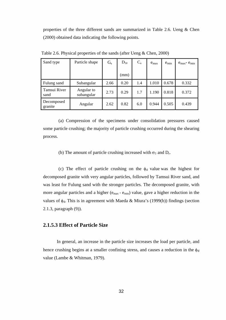
properties of the three different sands are summarized in Table 2.6. Ueng & Chen
(2000) obtained data indicating the following points.
Table 2.6. Physical properties of the sands (after Ueng & Chen, 2000)
Sand type Particle shape Gs D50
(mm)
Cu
emax
emin
emax- emin
Fulung sand Subangular 2.66 0.20 1.4 1.010 0.678 0.332
Tamsui River sand
Angular to subangular 2.73 0.29 1.7 1.190 0.818 0.372
Decomposed granite Angular 2.62 0.82 6.0 0.944 0.505 0.439
(a) Compression of the specimens under consolidation pressures caused
some particle crushing; the majority of particle crushing occurred during the shearing
process.
(b) The amount of particle crushing increased with σ3 and Dr.
(c) The effect of particle crushing on the φd value was the highest for
decomposed granite with very angular particles, followed by Tamsui River sand, and
was least for Fulung sand with the stronger particles. The decomposed granite, with
more angular particles and a higher (emax - emin) value, gave a higher reduction in the
values of φd. This is in agreement with Maeda & Miura’s (1999(b)) findings (section
2.1.3, paragraph (9)).
2.1.5.3 Effect of Particle Size
In general, an increase in the particle size increases the load per particle, and
hence crushing begins at a smaller confining stress, and causes a reduction in the φd
value (Lambe & Whitman, 1979).
32
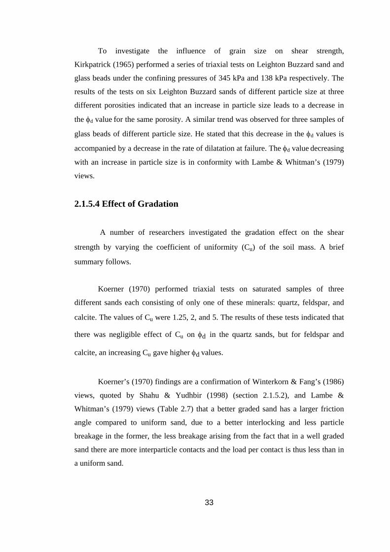
To investigate the influence of grain size on shear strength,
Kirkpatrick (1965) performed a series of triaxial tests on Leighton Buzzard sand and
glass beads under the confining pressures of 345 kPa and 138 kPa respectively. The
results of the tests on six Leighton Buzzard sands of different particle size at three
different porosities indicated that an increase in particle size leads to a decrease in
the φd value for the same porosity. A similar trend was observed for three samples of
glass beads of different particle size. He stated that this decrease in the φd values is
accompanied by a decrease in the rate of dilatation at failure. The φd value decreasing
with an increase in particle size is in conformity with Lambe & Whitman’s (1979)
views.
2.1.5.4 Effect of Gradation
A number of researchers investigated the gradation effect on the shear
strength by varying the coefficient of uniformity (Cu) of the soil mass. A brief
summary follows.
Koerner (1970) performed triaxial tests on saturated samples of three
different sands each consisting of only one of these minerals: quartz, feldspar, and
calcite. The values of Cu were 1.25, 2, and 5. The results of these tests indicated that
there was negligible effect of Cu on φd in the quartz sands, but for feldspar and
calcite, an increasing Cu gave higher φd values.
Koerner’s (1970) findings are a confirmation of Winterkorn & Fang’s (1986)
views, quoted by Shahu & Yudhbir (1998) (section 2.1.5.2), and Lambe &
Whitman’s (1979) views (Table 2.7) that a better graded sand has a larger friction
angle compared to uniform sand, due to a better interlocking and less particle
breakage in the former, the less breakage arising from the fact that in a well graded
sand there are more interparticle contacts and the load per contact is thus less than in
a uniform sand.
33
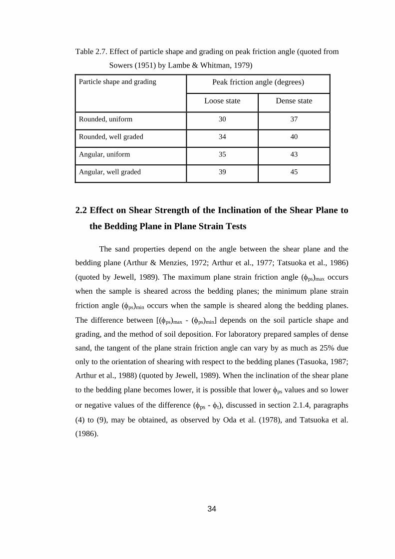
Table 2.7. Effect of particle shape and grading on peak friction angle (quoted from
Sowers (1951) by Lambe & Whitman, 1979)
Peak friction angle (degrees) Particle shape and grading
Loose state Dense state
Rounded, uniform 30 37
Rounded, well graded 34 40
Angular, uniform 35 43
Angular, well graded 39 45
2.2 Effect on Shear Strength of the Inclination of the Shear Plane to
the Bedding Plane in Plane Strain Tests
The sand properties depend on the angle between the shear plane and the
bedding plane (Arthur & Menzies, 1972; Arthur et al., 1977; Tatsuoka et al., 1986)
(quoted by Jewell, 1989). The maximum plane strain friction angle (φps)max occurs
when the sample is sheared across the bedding planes; the minimum plane strain
friction angle (φps)min occurs when the sample is sheared along the bedding planes.
The difference between [(φps)max - (φps)min] depends on the soil particle shape and
grading, and the method of soil deposition. For laboratory prepared samples of dense
sand, the tangent of the plane strain friction angle can vary by as much as 25% due
only to the orientation of shearing with respect to the bedding planes (Tasuoka, 1987;
Arthur et al., 1988) (quoted by Jewell, 1989). When the inclination of the shear plane
to the bedding plane becomes lower, it is possible that lower φps values and so lower
or negative values of the difference (φps - φt), discussed in section 2.1.4, paragraphs
(4) to (9), may be obtained, as observed by Oda et al. (1978), and Tatsuoka et al.
(1986).
34
2.3 Wedge Shear Tests
Unless otherwise stated, this section has been summarized from Mirata
(1991, 2003(a)).
The in situ wedge shear test (iswest) was developed (Mirata, 1974) as a
simpler means than the in situ large shear box test for measuring the shear strength of
unsaturated, fissured and/or stony clays. A different version of the iswest is the
cylindrical wedge shear test (cylwest) developed for enabling cylindrical samples of
clay (up to 10 mm dia.) taken from boreholes to be tested without the risk of entering
a test pit in an active landslide to perform an in situ test. The prismatic wedge shear
test (priswest) is a larger version of the cylwest, enabling prismatic specimens of
gravel, crushed rock or clay containing up to 40 mm particles to be tested, using a
portable frame. The test procedures for the last two versions are summarized in
sections 5.1.3 and 5.2.3.
2.3.1 Calculation of Stresses and Displacements
2.3.1.1 Introduction
The assumptions and calculations for the different types of analysis, which
will be explained below, based mainly on Fig. 2.14, are valid for all versions of the
wedge shear test. Basically the problem is one of summing up the normal and shear
components of all forces, and dividing these by the corrected area of the shear plane.
Differences in analysis arise in deciding which to take as the shear plane and whether
to consider the slight rotation β (Fig. 2.15) of the test mould during the test.
Distinction is made between three types of analysis explained in the following
sub-sections.
35
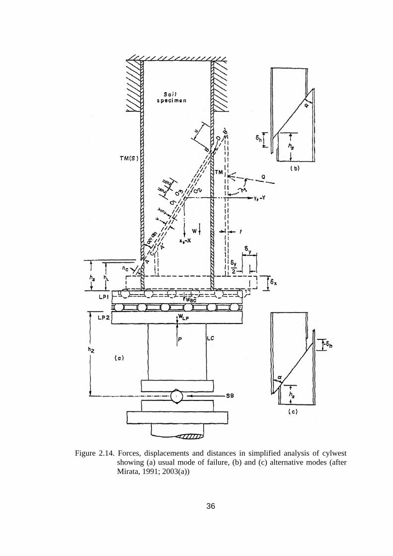
Figure 2.14. Forces, displacements and distances in simplified analysis of cylwest showing (a) usual mode of failure, (b) and (c) alternative modes (after Mirata, 1991; 2003(a))
36

Figure 2.15. Effect of mould rotation on the measured values of δx and δy in priswests
(after Mirata, 1991; 2003(a))
37
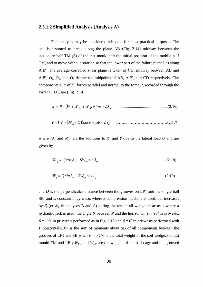
2.3.1.2 Simplified Analysis (Analysis A)
This analysis may be considered adequate for most practical purposes. The
soil is assumed to break along the plane AB (Fig. 2.14) midway between the
stationary half TM (S) of the test mould and the initial position of the mobile half
TM, and to move without rotation so that the lower part of the failure plane lies along
A′B′. The average corrected shear plane is taken as CD, midway between AB and
A′B′. O1, O2, and O3 denote the midpoints of AB, A′B′, and CD respectively. The
components X, Y of all forces parallel and normal to the force P, recorded through the
load cell LC, are (Fig. 2.14)
( ) qLPBC XsinWWWPX δθ +++−= .................................................(2.16)
( )( ) qB YPcosD/MWY δµθ +++= …….....………….……………(2.17)
where δXq and δYq are the additions to X and Y due to the lateral load Q and are
given by
qqnqq sinSWcosQX λλδ −= ……….........……..…………………...(2.18)
qqnqq cosSWsinQY λλδ += …………..................………………...(2.19)
and D is the perpendicular distance between the grooves on LP1 and the single ball
SB, and is constant in cylwests where a compression machine is used, but increases
by δx (or δxo in analyses B and C) during the test in all wedge shear tests where a
hydraulic jack is used; the angle θ between P and the horizontal (θ = 90o in cylwests;
θ = -90o in priswests performed as in Fig. 2.15 and θ = 0o in priswests performed with
P horizontal); MB is the sum of moments about SB of all components between the
grooves of LP1 and SB when θ = 0o; W is the total weight of the soil wedge, the test
mould TM and LP1; WBC and WLP are the weights of the ball cage and the grooved
38
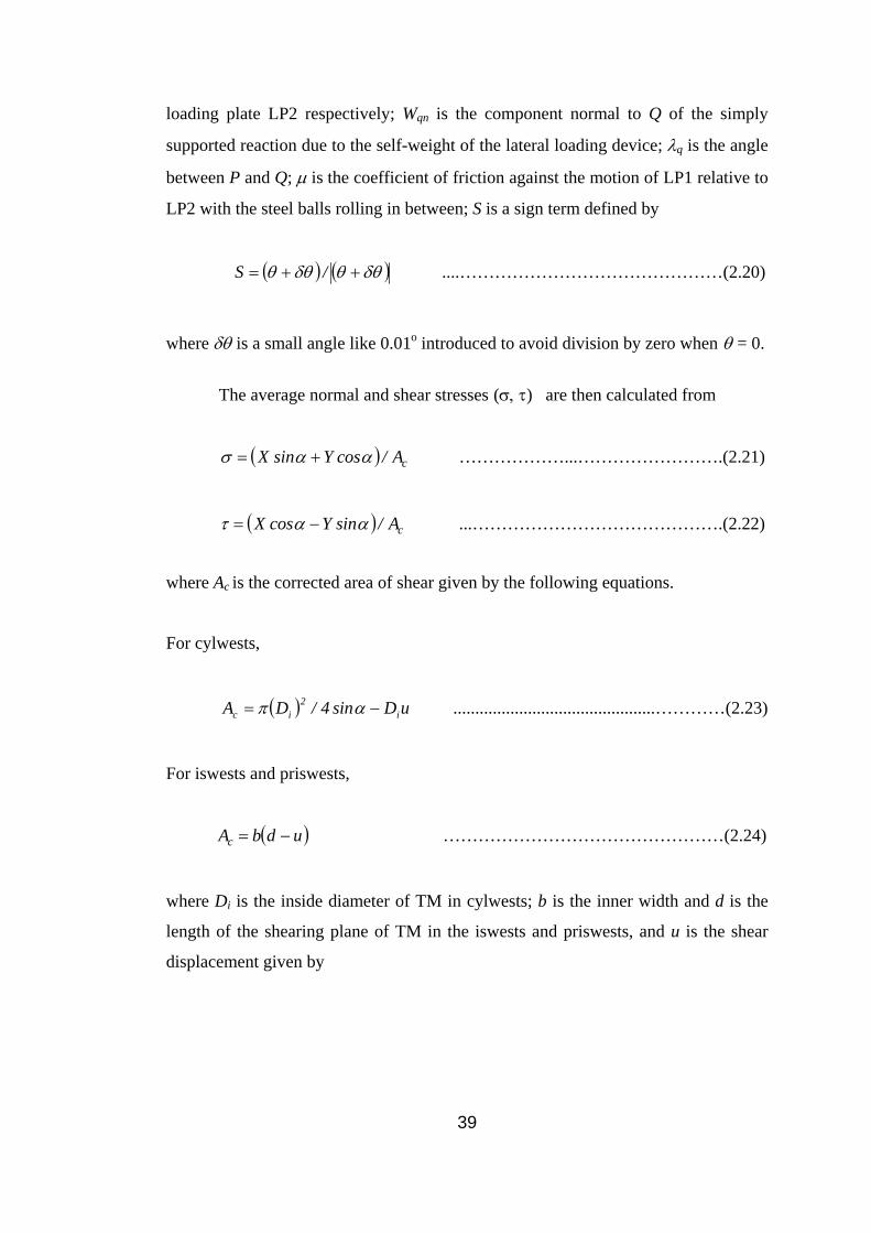
loading plate LP2 respectively; Wqn is the component normal to Q of the simply
supported reaction due to the self-weight of the lateral loading device; λq is the angle
between P and Q; µ is the coefficient of friction against the motion of LP1 relative to
LP2 with the steel balls rolling in between; S is a sign term defined by
( ) ( )δθθδθθ ++= /S ....………………………………………(2.20)
where δθ is a small angle like 0.01o introduced to avoid division by zero when θ = 0.
The average normal and shear stresses (σ, τ) are then calculated from
( cA/cosYsinX )αασ += ………………...…………………….(2.21)
( cA/sinYcosX )αατ −= ...…………………………………….(2.22) where Ac is the corrected area of shear given by the following equations. For cylwests,
( ) uDsin4/DA i2
ic −= απ ..............................................…………(2.23)
For iswests and priswests,
( )udbAc −= …………………………………………(2.24)
where Di is the inside diameter of TM in cylwests; b is the inner width and d is the
length of the shearing plane of TM in the iswests and priswests, and u is the shear
displacement given by
39

αδαδ sincosu yx += ……...................………………………(2.25)
where δx and δy are the displacements measured in the positive directions of X and y
(Fig. 2.14), respectively. The normal displacement v is given by
αδαδ sincosv xy −= ..............................................................(2.26)
where positive values of v indicate dilatation. α = αn, the nominal angle between P
and the shearing plane of TM (Fig. 2.15) in priswests and iswests, and in cylwests
where the specimen fails as in Fig. 2.14(a). In cylwests on clays, failure can
sometimes occur as in Fig. 2.14(b) or (c), in which case α is calculated from the
geometry of the failure plane.
2.3.1.3 Average Shear Plane Analysis (Analysis B)
In this analysis, the average shear plane is assumed to be the same as in
Analysis A, except that the effect of the slight rotation β of the mould is taken into
account. The average shear and normal displacements (u , v respectively), and β are
calculated as explained by Mirata (1991). θ in equations (2.16) and (2.17) is then
replaced by βθθ +=r , and u in equations (2.23) and (2.24) by u . The value of α is
unaltered, implying that both P and the average shear plane rotate by β.
2.3.1.4 True Shear Plane Analysis (Analysis C)
The rotation β is calculated as in analysis B, but shear is assumed to take
place initially between the trailing tip A1 of TM and the point B1 which represents
the opposite tip of TM (S) (Fig. 2.15). The angle iα between A1B1 and the initial
direction of P, and the length 11BA (Fig. 2.16) are calculated as explained by Mirata
(1991).
40

Figure 2.16. Pre-failure deformation of a plastic clay in cylwest (after Mirata, 1991; 2003(a))
41

The angle αr between the rotated position of P and A1B1 (Fig. 2.16), and the
equivalent shear displacement 1u are given by
β−α=α ir ......………………………………………………………(2.27)
111 2 BAsin/du iyb −= α ......………………………………………….(2.28)
where dyb is defined as ( 2/cos/nsind ncn )α−α in priswests and iswests (where nc
is the initial clearance between the shearing planes of the two halves of the priswest
box, and is equal to 0 for iswests), and as (Di / 2) in cylwests. Equations (2.23) and
(2.24) are then replaced by equations (2.29) and (2.30), and α in equations (2.21) and
(2.22) is replaced by αr.
For cylwests,
( ) iybc Dusin/dA 12 −= απ ................................................(2.29)
For iswests and priswests,
( )12 usin/dbA iybc −= α ...................................................(2.30)
After the peak strength is reached, further movement of the soil wedge is
assumed to take place in the general direction of the failure plane formed at peak
strength, but any further changes in β to be reflected equally to the direction of P
and the orientation of the failure plane. So 1u in equations (2.29) and (2.30) is
replaced by u obtained as in analysis B, and αi and αr are assumed to remain fixed
at the values at peak strength.
42
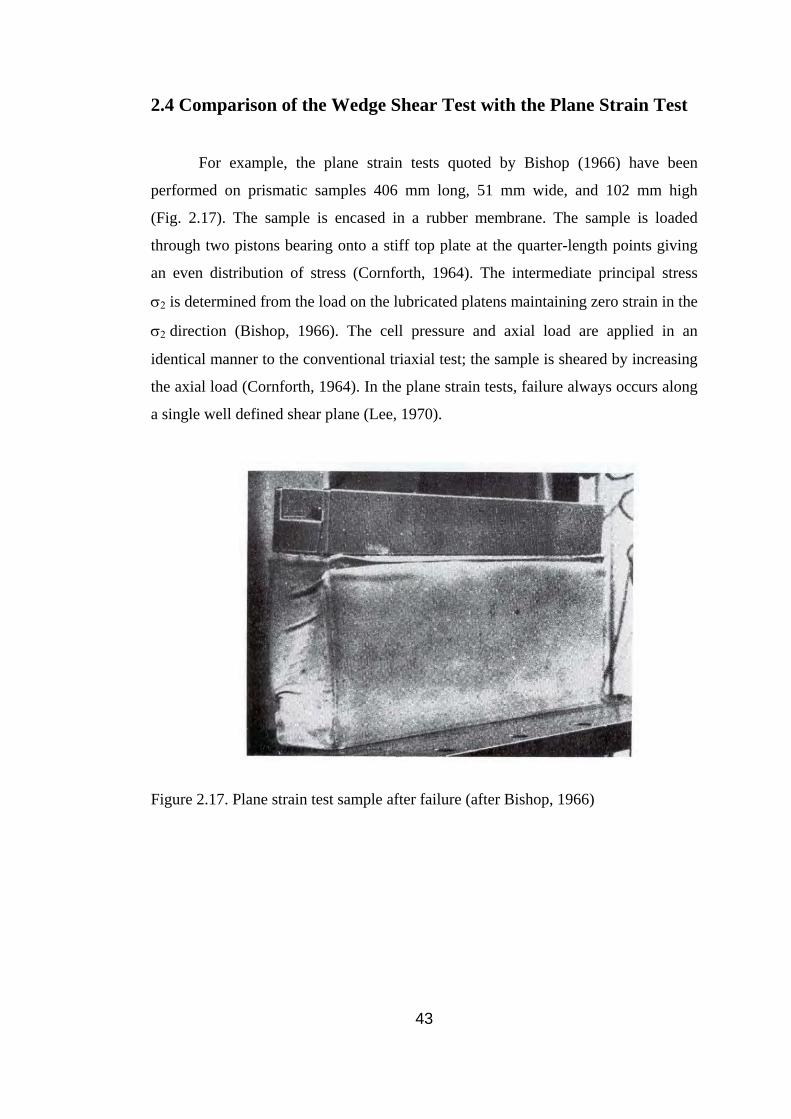
2.4 Comparison of the Wedge Shear Test with the Plane Strain Test
For example, the plane strain tests quoted by Bishop (1966) have been
performed on prismatic samples 406 mm long, 51 mm wide, and 102 mm high
(Fig. 2.17). The sample is encased in a rubber membrane. The sample is loaded
through two pistons bearing onto a stiff top plate at the quarter-length points giving
an even distribution of stress (Cornforth, 1964). The intermediate principal stress
σ2 is determined from the load on the lubricated platens maintaining zero strain in the
σ2 direction (Bishop, 1966). The cell pressure and axial load are applied in an
identical manner to the conventional triaxial test; the sample is sheared by increasing
the axial load (Cornforth, 1964). In the plane strain tests, failure always occurs along
a single well defined shear plane (Lee, 1970).
Figure 2.17. Plane strain test sample after failure (after Bishop, 1966)
43
The following has been taken from Mirata (2003(b)).
In the prismatic wedge shear test (priswest), each half of the sample, such as
seen in Fig. 2.15, is enclosed in a 10 - mm thick steel mould; the lateral yield of the
sample is thus prevented except along the relatively small gap (Tables 5.9 to 5.14,
column 3) between the two halves of the mould. No rubber membrane is used. The
sample is sheared by applying a relatively small lateral load (analogous to the cell
pressure in Fig. 2.17), and increasing the main load P (analogous to the axial load in
Fig. 2.17). The angle between the shear plane and the main load is restricted by the
test mould used, and the distribution of stress on the faces of the sample, although
capable of being controlled to some extent by applying an initial eccentricity to P, is
not uniform (see Tables 5.9 to 5.14, columns 5, 12, and 19). The initial shear plane
area is 300 mm x 300 mm, and the test is evaluated on the basis of average stresses
on this plane, as in the conventional shear box test.
In the cylindrical wedge shear test (cylwest), loading is effected in a similar
way to the priswest, but the sheared wedge is part of a cylinder, and the shear plane
is initially elliptical. On the other hand, the inclination of the shear plane to the
layering during sample placement in the cylwest using an αn = 30o test mould is
closer to that in the plane strain test (Fig. 2.17). In the priswest this inclination is
lower, but can be improved by modifying the test mould (Fig. 5.9(b)) so that the side
of the mould on which the main load is applied becomes the removable lid.
It is seen that the wedge shear test is similar but not identical with the
conventional plane strain test.
44
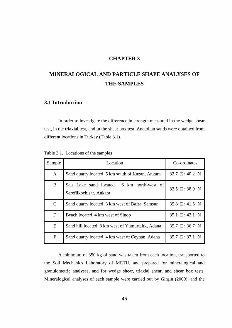
CHAPTER 3
MINERALOGICAL AND PARTICLE SHAPE ANALYSES OF
THE SAMPLES
3.1 Introduction
In order to investigate the difference in strength measured in the wedge shear
test, in the triaxial test, and in the shear box test, Anatolian sands were obtained from
different locations in Turkey (Table 3.1).
Table 3.1. Locations of the samples
Sample Location Co-ordinates
A Sand quarry located 5 km south of Kazan, Ankara 32.7o E ; 40.2o N
B Salt Lake sand located 6 km north-west of
Şereflikoçhisar, Ankara 33.5o E ; 38.9o N
C Sand quarry located 3 km west of Bafra, Samsun 35.8o E ; 41.5o N
D Beach located 4 km west of Sinop 35.1o E ; 42.1o N
E Sand hill located 8 km west of Yumurtalık, Adana 35.7o E ; 36.7o N
F Sand quarry located 4 km west of Ceyhan, Adana 35.7o E ; 37.1o N
A minimum of 350 kg of sand was taken from each location, transported to
the Soil Mechanics Laboratory of METU, and prepared for mineralogical and
granulometric analyses, and for wedge shear, triaxial shear, and shear box tests.
Mineralogical analyses of each sample were carried out by Girgin (2000), and the
45
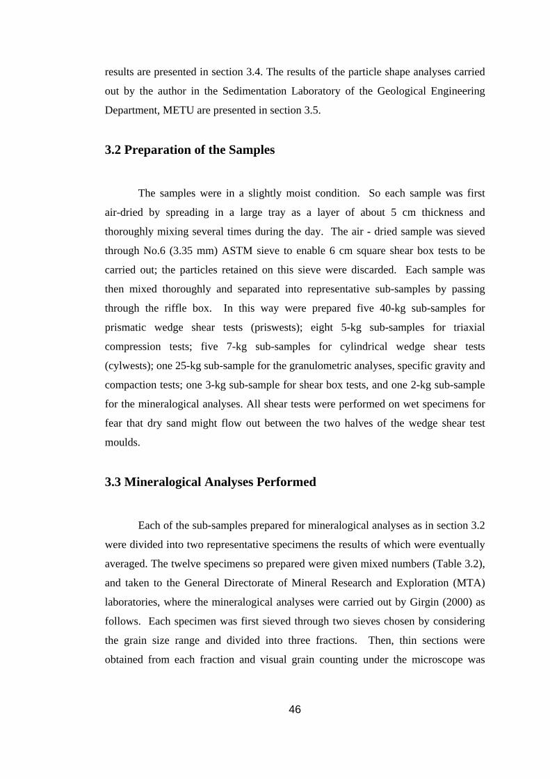
results are presented in section 3.4. The results of the particle shape analyses carried
out by the author in the Sedimentation Laboratory of the Geological Engineering
Department, METU are presented in section 3.5.
3.2 Preparation of the Samples
The samples were in a slightly moist condition. So each sample was first
air-dried by spreading in a large tray as a layer of about 5 cm thickness and
thoroughly mixing several times during the day. The air - dried sample was sieved
through No.6 (3.35 mm) ASTM sieve to enable 6 cm square shear box tests to be
carried out; the particles retained on this sieve were discarded. Each sample was
then mixed thoroughly and separated into representative sub-samples by passing
through the riffle box. In this way were prepared five 40-kg sub-samples for
prismatic wedge shear tests (priswests); eight 5-kg sub-samples for triaxial
compression tests; five 7-kg sub-samples for cylindrical wedge shear tests
(cylwests); one 25-kg sub-sample for the granulometric analyses, specific gravity and
compaction tests; one 3-kg sub-sample for shear box tests, and one 2-kg sub-sample
for the mineralogical analyses. All shear tests were performed on wet specimens for
fear that dry sand might flow out between the two halves of the wedge shear test
moulds.
3.3 Mineralogical Analyses Performed
Each of the sub-samples prepared for mineralogical analyses as in section 3.2
were divided into two representative specimens the results of which were eventually
averaged. The twelve specimens so prepared were given mixed numbers (Table 3.2),
and taken to the General Directorate of Mineral Research and Exploration (MTA)
laboratories, where the mineralogical analyses were carried out by Girgin (2000) as
follows. Each specimen was first sieved through two sieves chosen by considering
the grain size range and divided into three fractions. Then, thin sections were
obtained from each fraction and visual grain counting under the microscope was
46

made on the sections. The mineralogical composition of the samples so obtained is
presented in the following sections.
Table 3.2. Specimen numbers for mineralogical analyses
Sample Mineralogical analysis specimen numbers
A S5, S11
B S2, S9
C S1, S7
D S4, S10
E S6, S8
F S3, S12
3.4 Results of Mineralogical Analyses:
In this section the following notation has been used:
MRF: metamorphic rock fragments;
SRF: sedimentary rock fragments;
EAURF: extensively altered ultrabasic rock fragments;
EIRF: extrusive igneous rock fragments;
IIRF: intrusive igneous rock fragments;
TF: tuffaceous fragments.
The relative contribution to shear strength, based on the assessment by
Norman (2000(b)), was indicated as follows: (+): tending to increase shear strength,
(-): tending to decrease shear strength and (+-): effect on shear strength unknown.
The mineralogical composition of the samples and relative contribution to
strength of the different ingredients, listed in order of abundance in any one category,
are given in Tables 3.3 to 3.14.
47
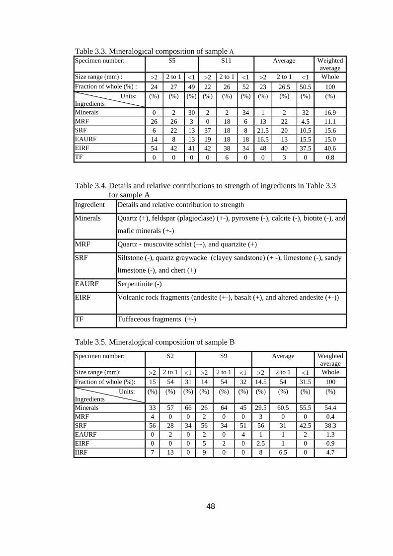
Table 3.3. Mineralogical composition of sample A Specimen number: S5 S11 Average Weighted
average Size range (mm) : >2 2 to 1 <1 >2 2 to 1 <1 >2 2 to 1 <1 Whole Fraction of whole (%) : 24 27 49 22 26 52 23 26.5 50.5 100 Units: Ingredients
(%) (%) (%) (%) (%) (%) (%) (%) (%) (%)
Minerals 0 2 30 2 2 34 1 2 32 16.9 MRF 26 26 3 0 18 6 13 22 4.5 11.1 SRF 6 22 13 37 18 8 21.5 20 10.5 15.6 EAURF 14 8 13 19 18 18 16.5 13 15.5 15.0 EIRF 54 42 41 42 38 34 48 40 37.5 40.6 TF 0 0 0 0 6 0 0 3 0 0.8 Table 3.4. Details and relative contributions to strength of ingredients in Table 3.3 for sample A Ingredient Details and relative contribution to strength
Minerals Quartz (+), feldspar (plagioclase) (+-), pyroxene (-), calcite (-), biotite (-), and
mafic minerals (+-)
MRF Quartz - muscovite schist (+-), and quartzite (+)
SRF Siltstone (-), quartz graywacke (clayey sandstone) (+ -), limestone (-), sandy
limestone (-), and chert (+)
EAURF Serpentinite (-)
EIRF Volcanic rock fragments (andesite (+-), basalt (+), and altered andesite (+-))
TF Tuffaceous fragments (+-)
Table 3.5. Mineralogical composition of sample B
Specimen number: S2 S9 Average Weighted average
Size range (mm): >2 2 to 1 <1 >2 2 to 1 <1 >2 2 to 1 <1 Whole Fraction of whole (%): 15 54 31 14 54 32 14.5 54 31.5 100 Units: Ingredients
(%) (%) (%) (%) (%) (%) (%) (%) (%) (%)
Minerals 33 57 66 26 64 45 29.5 60.5 55.5 54.4 MRF 4 0 0 2 0 0 3 0 0 0.4 SRF 56 28 34 56 34 51 56 31 42.5 38.3 EAURF 0 2 0 2 0 4 1 1 2 1.3 EIRF 0 0 0 5 2 0 2.5 1 0 0.9 IIRF 7 13 0 9 0 0 8 6.5 0 4.7
48
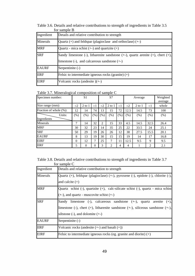
Table 3.6. Details and relative contributions to strength of ingredients in Table 3.5 for sample B Ingredient Details and relative contribution to strength
Minerals Quartz (+) and feldspar (plagioclase and orthoclase) (+-)
MRF Quartz - mica schist (+-) and quartzite (+)
SRF Sandy limestone (-), litharenite sandstone (+-), quartz arenite (+), chert (+),
limestone (-), and calcareous sandstone (+-)
EAURF Serpentinite (-)
IIRF Felsic to intermediate igneous rocks (granite) (+)
EIRF Volcanic rocks (andesite )(+-)
Table 3.7. Mineralogical composition of sample C Specimen number: S1 S7 Average Weighted
average Size range (mm): >2 2 to 1 <1 >2 2 to 1 <1 >2 2 to 1 <1 whole Fraction of whole (%): 12 14 74 13 15 72 12.5 14.5 73 100 Units: Ingredients
(%) (%) (%) (%) (%) (%) (%) (%) (%) (%)
Minerals 7 14 32 2 15 33 4.5 14.5 32.5 26.4 MRF 30 32 23 14 35 25 22 33.5 24 25.1 SRF 50 29 19 26 26 12 38 27.5 15.5 20.1 EAURF 8 13 19 30 15 15 19 14 17 16.8 EIRF 0 12 7 25 7 11 12.5 9.5 9 9.5 IIRF 5 0 0 3 2 4 4 1 2 2.1 Table 3.8. Details and relative contributions to strength of ingredients in Table 3.7 for sample C Ingredient Details and relative contribution to strength
Minerals Quartz (+), feldspar (plagioclase) (+-), pyroxene (-), epidote (-), chlorite (-),
and calcite (+)
MRF Quartz schist (-), quartzite (+), calc-silicate schist (-), quartz - mica schist
(+-), and quartz - muscovite schist (+-)
SRF Sandy limestone (-), calcareous sandstone (+-), quartz arenite (+),
limestone (-), chert (+), litharenite sandstone (+-), siliceous sandstone (+-),
siltstone (-), and dolomite (+-)
EAURF Serpentinite (-)
IIRF Volcanic rocks (andesite (+-) and basalt (+))
EIRF Felsic to intermediate igneous rocks (eg. granite and diorite) (+)
49

Table 3.9. Mineralogical composition of sample D Specimen number: S4 S10 Average Weighted
average Size range (mm): >0.5 < 0.5 >0.5 0.5 to 0.25 <.25 >0.5 < 0.5 whole Fraction of whole (%): 82 18 2 94 4 42 58 100 Units: Ingredients
(%) (%) (%) (%) (%) (%) (%) (%)
Minerals 53 42 53 28 51 53 41 46.0 MRF 5 19 18 20 11 11.5 17 14.7 SRF 34 28 27 41 29 30.5 31 30.8 EAURF 4 11 2 11 9 3 11 7.7 EIRF 4 0 0 0 0 2 0 0.8 Table 3.10. Details and relative contributions to strength of ingredients in Table 3.9 for sample D Ingredient Details and relative contribution to strength
Minerals Quartz (+), feldspar (plagioclase and orthoclase) (+-), pyroxene(-),
calcite (-), and epidote (-)
MRF Quartz - mica schist (+-), and quartzite (+)
SRF Limestone (-), sandy limestone (-), and siltstone (-)
EAURF Serpentinite (-)
EIRF Volcanic rock fragments (+-)
Table 3.11. Mineralogical composition of sample E Specimen number: S6 S8 Average Weighted
average Size range (mm): >.5 .5 to .25 <.25 >.5 .5 to .25 <.25 >.5 .5 to .25 < .25 whole Fraction of whole (%): 14 64 22 13 66 21 13.5 65 21.5 100 Units: Ingredients
(%) (%) (%) (%) (%) (%) (%) (%) (%) (%)
Minerals 5 23 27 6 21 31 5.5 22 29 21.3 SRF 90 67 55 87 67 57 88.5 67 56 67.5 EAURF 5 10 18 7 12 8 6 11 13 10.8 EIRF 0 0 0 0 0 4 0 0 2 0.4
50

Table 3.12. Details and relative contributions to strength of ingredients in Table 3.11 for sample E
Ingredient Details and relative contribution to strength
Minerals Quartz (+), feldspar (plagioclase) (+-), epidote (-), and mafic minerals (+-)
SRF Sandy limestone (-), litharenite sandstone (+-), limestone (-), chert (+),
siltstone (-), quartz arenite (+), dolomitic limestone (-), and fossil fragments
(-)
EAURF Serpentinite (-)
EIRF Volcanic rock fragments (andesite (+-))
Table 3.13. Mineralogical composition of sample F Specimen number: S3 S12 Average Weighted
average Size range (mm): >2 2 to 1 <1 >2 2 to 1 <1 >2 2 to 1 <1 whole Fraction of whole (%): 2 4 94 2 4 94 2 4 94 100 Units: Ingredients
(%) (%) (%) (%) (%) (%) (%) (%) (%) (%)
Minerals 0 7 26 2 14 38 1 10.5 32 30.5 MRF 6 11 2 13 12 6 9.5 11.5 4 4.4 SRF 53 38 45 34 23 32 43.5 30.5 38.5 38.2 EAURF 27 24 19 32 42 17 29.5 33 18 18.8 EIRF 12 16 4 17 7 7 14.5 11.5 5.5 5.9 IIRF 3 4 4 2 2 0 2.5 3 2 2.2
Table 3.14. Details and relative contributions to strength of ingredients in Table 3.13 for sample F
Ingredient Details and relative contribution to strength
Minerals Quartz (+), feldspar (+-), calcite (-), pyroxene (-), biotite (-), and epidote (-)
MRF Quartz - mica schist (+-), quartz - muscovite schist (+-)
SRF Clayey siltstone (-), quartz arenite (+), chert (+), litharenite sandstone (+-),
limestone (-), siltstone (-), and sandy limestone (-)
EAURF Extensively altered and silicified ultrabasic rock fragments (-)
EIRF Volcanic rock fragments (andesite (+-) and altered andesite (+-))
IIRF Felsic to intermediate igneous rocks (granite and granodiorite /diorite) (+)
The mineralogical analyses show that each sample contains both single
mineral particles (quartz, feldspar, calcite, epidote, etc) and rock particles (quartz
arenite, quartzite, limestone, etc.), which have different contribution to strength. In
51

any one category, the relative contribution to strength of the different ingredients is
listed in order of abundance, but the individual percentages of these ingredients are
unknown, yielding unpredictable contribution to strength. To determine the effect on
strength of the mineral composition of the sands, more detailed analyses seem to be
required, including determination of individual percentages of each ingredient
(which was not possible in this study).
3.5 Results of Particle Shape Analyses
Particle shape analyses of each sample were carried out in the Sedimentation
Laboratory of the Geological Engineering Department, METU.
Projection was used for determining grain morphology (particle shape)
quantified by the roundness RF and sphericity SR, defined in section 2.1.5.1. The
methods given by Dobkins & Folk (1970) and Riley (1941), given in section 2.1.5.1,
were used for RF and SR respectively as follows. RF and SR were calculated for 60
grains projected for each of the samples by measuring selected grain axes (dk, di, and
dc (Fig. 2.10)); average values of RF and SR for each sample were taken. The results
of particle shape analyses so obtained are given in Table 3.15.
Table 3.15. The results of particle shape analyses of each sample
Sample RF SR
A 0.25 0.78 B 0.22 0.80 C 0.21 0.78 D 0.30 0.77 E 0.33 0.80 F 0.34 0.79
According to the classification given in section 2.1.5.1 (Table 2.3), samples
A, B, and C consist of angular particles; samples D, E, and F consist of subangular
particles. Also, according to the chart given in section 2.1.5.1 (Fig. 2.11), the SR
values indicate grains of high sphericity.
52
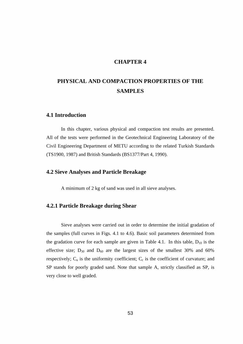
CHAPTER 4
PHYSICAL AND COMPACTION PROPERTIES OF THE
SAMPLES
4.1 Introduction
In this chapter, various physical and compaction test results are presented.
All of the tests were performed in the Geotechnical Engineering Laboratory of the
Civil Engineering Department of METU according to the related Turkish Standards
(TS1900, 1987) and British Standards (BS1377/Part 4, 1990).
4.2 Sieve Analyses and Particle Breakage
A minimum of 2 kg of sand was used in all sieve analyses.
4.2.1 Particle Breakage during Shear
Sieve analyses were carried out in order to determine the initial gradation of
the samples (full curves in Figs. 4.1 to 4.6). Basic soil parameters determined from
the gradation curve for each sample are given in Table 4.1. In this table, D10 is the
effective size; D30 and D60 are the largest sizes of the smallest 30% and 60%
respectively; Cu is the uniformity coefficient; Cc is the coefficient of curvature; and
SP stands for poorly graded sand. Note that sample A, strictly classified as SP, is
very close to well graded.
53
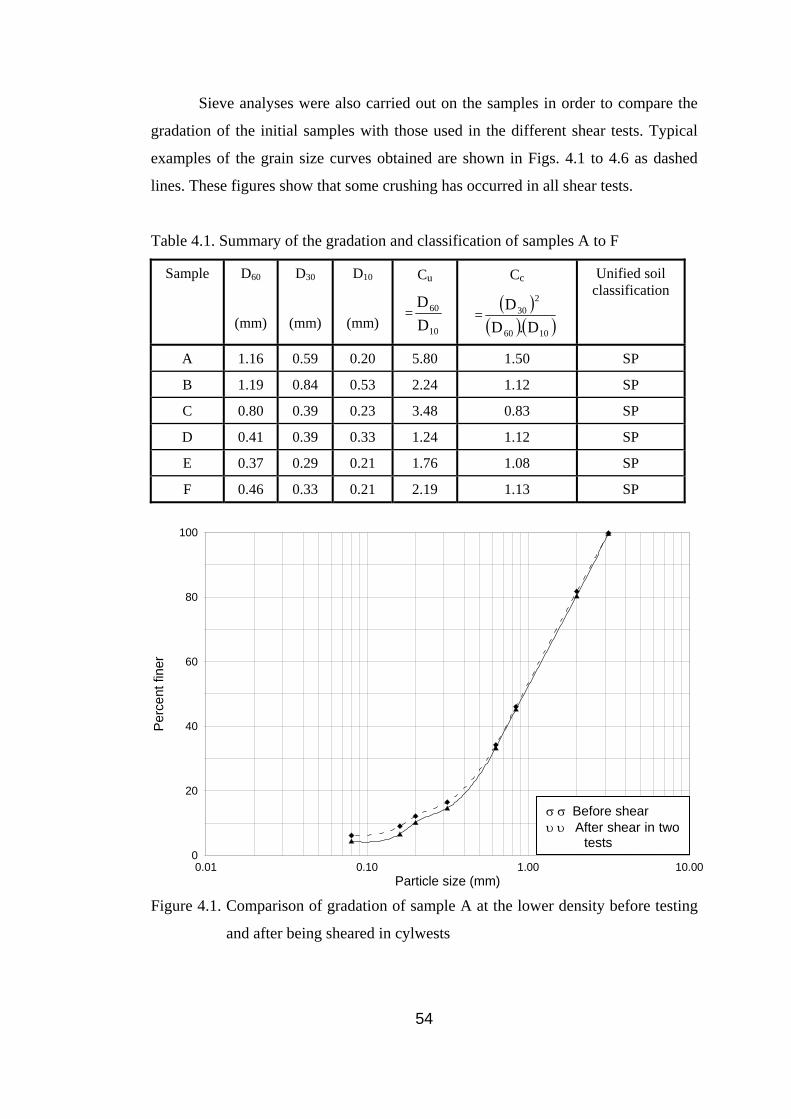
Sieve analyses were also carried out on the samples in order to compare the
gradation of the initial samples with those used in the different shear tests. Typical
examples of the grain size curves obtained are shown in Figs. 4.1 to 4.6 as dashed
lines. These figures show that some crushing has occurred in all shear tests.
Table 4.1. Summary of the gradation and classification of samples A to F
Sample D60
(mm)
D30
(mm)
D10
(mm)
Cu
=10
60
DD
Cc
=( )
( )( )1060
230
D.DD
Unified soil classification
A 1.16 0.59 0.20 5.80 1.50 SP
B 1.19 0.84 0.53 2.24 1.12 SP
C 0.80 0.39 0.23 3.48 0.83 SP
D 0.41 0.39 0.33 1.24 1.12 SP
E 0.37 0.29 0.21 1.76 1.08 SP
F 0.46 0.33 0.21 2.19 1.13 SP
0.01 0.10 1.00 10.00Particle size (mm)
0
20
40
60
80
100
Perc
ent f
iner
σ σ Before shear υ υ After shear in two
tests
Figure 4.1. Comparison of gradation of sample A at the lower density before testing
and after being sheared in cylwests
54
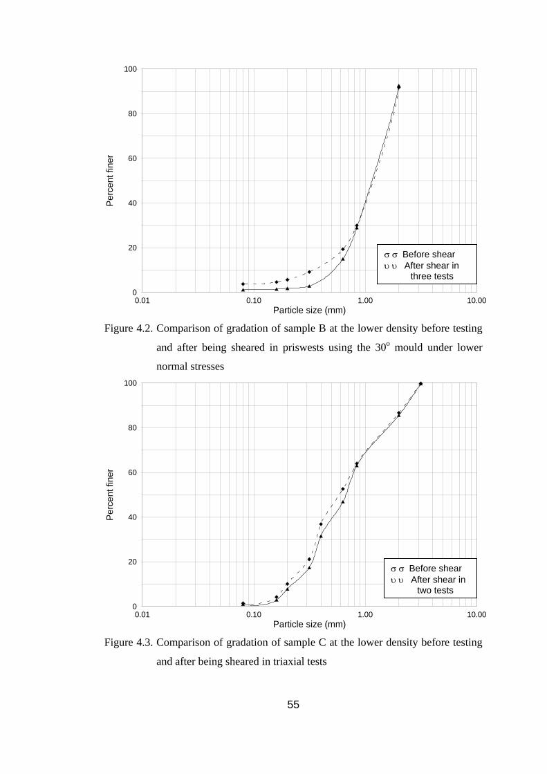
0.01 0.10 1.00 10.00Particle size (mm)
0
20
40
60
80
100
Perc
ent f
iner
σ σ Before shear υ υ After shear in
three tests
Figure 4.2. Comparison of gradation of sample B at the lower density before testing
and after being sheared in priswests using the 30o mould under lower
normal stresses
0.01 0.10 1.00 10.00Particle size (mm)
0
20
40
60
80
100
Perc
ent f
iner
σ σ Before shear υ υ After shear in
two tests
Figure 4.3. Comparison of gradation of sample C at the lower density before testing
and after being sheared in triaxial tests
55

0.01 0.10 1.00Particle size (mm)
0
20
40
60
80
100
Perc
ent f
iner
σ σ Before shear υ υ After shear in
two tests
Figure 4.4. Comparison of gradation of sample D at the higher density before testing
and after being sheared in cylwests
0.01 0.10 1.00 10.00Particle size (mm)
0
20
40
60
80
100
Perc
ent f
iner
σ σ Before shear υ υ After shear in
three tests
Figure 4.5. Comparison of gradation of sample E at the higher density before testing
and after being sheared in priswests using the 40o mould under higher
normal stresses
56

0.01 0.10 1.00 10.00Particle size (mm)
0
20
40
60
80
100
Perc
ent f
iner
σ σ Before shear υ υ After shear in
two tests
Figure 4.6. Comparison of gradation of sample F at the higher density before testing
and after being sheared in triaxial tests
The values of Marsal’s (1967) breakage factor Bg (Appendix C) were
calculated from the initial and final gradation of samples A to F at the lower and
higher densities (Table 4.2). In this table, the test numbers in columns 2 to 9 refer to
the test numbers in Tables 5.1, 5.8, and 6.1 for the cylwests, priswests, and triaxial
tests respectively.
Comparing the values of Bg of all samples at the lower density
(Table 4.2, columns 2 to 5) both under the lower and higher ranges of normal stress
σ, the values of Bg for samples A to C are smaller than those for samples D to F. This
indicates that samples A to C have particles exhibiting relatively higher resistance to
crushing than samples D to F.
Generally, for sands with particles of angular shapes, particle crushing can be
quite significant even under low pressure (Ueng & Chen, 2000) (section 2.1.5.2).
However, in this study, more particle crushing occurred in samples with subangular
particles (samples D to F) compared to the samples with angular particles (samples A
57

Table 4.2. Breakage factors calculated from the initial and final gradation of samples A to F after different shear test
1 2 3 4 5 6 7 8 9
Breakage factors of samples A to F at the lower density Breakage factors of samples D to F at the higher density Sample
Cylwests Priswests Triaxial tests Cylwests Priswests Triaxial tests
A After test 4
Bg = 3.1 %
After test 3
Bg = 4.2 %
After test 6
Bg = 4.7 %
After test 7
Bg = 4.5 % ... … … …
B After test 4
Bg = 6.6 %
After test 3
Bg= 6.2 %
After test 6
Bg = 7.0 %
After test 7
Bg = 6.7 % … … … …
C After test 4
Bg = 7.6 %
After test 5
Bg = 5.8 %
After test 6
Bg = 8.3 %
After test 7
Bg = 7.9 % … … … …
D After test 4
Bg = 13.7 %
After test 5
Bg = 14.8 %
After test 6
Bg = 19.1 %
After test 7
Bg = 17.7 %
After test 4
Bg = 39.5 %
After test 3
Bg = 44.5 %
After test 6
Bg = 46.4 %
After test 6
Bg = 40.7 %
E After test 4
Bg = 13.8 %
After test 5
Bg = 20.8 %
After test 6
Bg = 23.7 %
After test 7
Bg = 21.9 %
After test 4
Bg = 25.7 %
After test 3
Bg = 27.2 %
After test 6
Bg = 28.0 %
After test 6
Bg = 26.7 %
F After test 4
Bg = 10.2 %
After test 5
Bg = 11.3 %
After test 6
Bg = 14.1 %
After test 7
Bg = 14.5 %
After test 4
Bg = 18.5 %
After test 3
Bg = 18.8 %
After test 6
Bg = 22.5 %
After test 6
Bg = 24.8 %
58
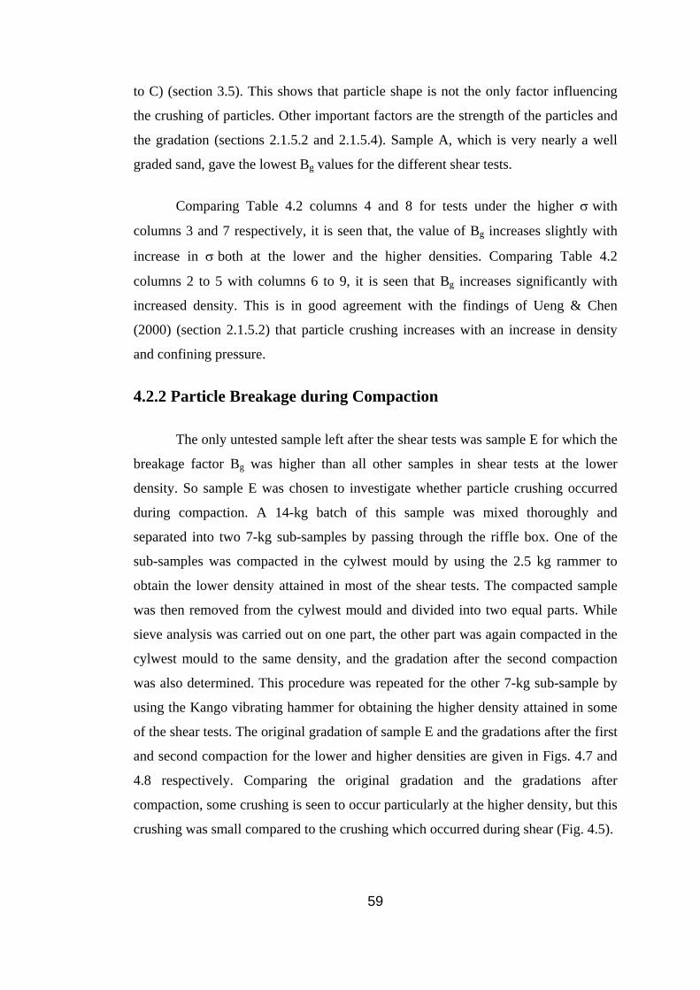
to C) (section 3.5). This shows that particle shape is not the only factor influencing
the crushing of particles. Other important factors are the strength of the particles and
the gradation (sections 2.1.5.2 and 2.1.5.4). Sample A, which is very nearly a well
graded sand, gave the lowest Bg values for the different shear tests.
Comparing Table 4.2 columns 4 and 8 for tests under the higher σ with
columns 3 and 7 respectively, it is seen that, the value of Bg increases slightly with
increase in σ both at the lower and the higher densities. Comparing Table 4.2
columns 2 to 5 with columns 6 to 9, it is seen that Bg increases significantly with
increased density. This is in good agreement with the findings of Ueng & Chen
(2000) (section 2.1.5.2) that particle crushing increases with an increase in density
and confining pressure.
4.2.2 Particle Breakage during Compaction
The only untested sample left after the shear tests was sample E for which the
breakage factor Bg was higher than all other samples in shear tests at the lower
density. So sample E was chosen to investigate whether particle crushing occurred
during compaction. A 14-kg batch of this sample was mixed thoroughly and
separated into two 7-kg sub-samples by passing through the riffle box. One of the
sub-samples was compacted in the cylwest mould by using the 2.5 kg rammer to
obtain the lower density attained in most of the shear tests. The compacted sample
was then removed from the cylwest mould and divided into two equal parts. While
sieve analysis was carried out on one part, the other part was again compacted in the
cylwest mould to the same density, and the gradation after the second compaction
was also determined. This procedure was repeated for the other 7-kg sub-sample by
using the Kango vibrating hammer for obtaining the higher density attained in some
of the shear tests. The original gradation of sample E and the gradations after the first
and second compaction for the lower and higher densities are given in Figs. 4.7 and
4.8 respectively. Comparing the original gradation and the gradations after
compaction, some crushing is seen to occur particularly at the higher density, but this
crushing was small compared to the crushing which occurred during shear (Fig. 4.5).
59
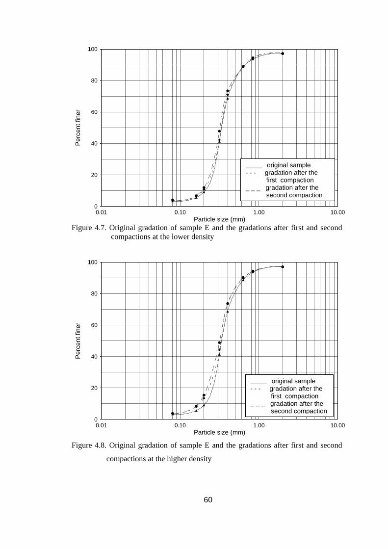
0.01 0.10 1.00 10.00Particle size (mm)
0
20
40
60
80
100
Perc
ent f
iner
_____ original sample - - - gradation after the
first compaction _ _ _ gradation after the
second compaction
Figure 4.7. Original gradation of sample E and the gradations after first and second compactions at the lower density
0.01 0.10 1.00 10.00Particle size (mm)
0
20
40
60
80
100
Perc
ent f
iner
_____ original sample - - - gradation after the
first compaction _ _ _ gradation after the
second compaction
Figure 4.8. Original gradation of sample E and the gradations after first and second
compactions at the higher density
60

4.3 Density Tests
4.3.1 Maximum Density Tests
The maximum density tests were performed on each sample generally
following the procedure given in the British Standards (BS 1377, 1990).
This method is suitable for sands containing a small amount of material
passing a 63-µm test sieve, and up to 10 % of fine gravel passing a 6.3-mm test
sieve. The soil is compacted in a 1-litre mould (105 mm inside diameter, 115.5 mm
high) under water using an electric vibrating hammer. In this study, a mould, 152
mm in diameter, 115 mm high was used.
The sample prepared as in section 3.2 was mixed thoroughly on a large metal
tray, and divided by riffling into two representative portions of about 5 kg each. Each
sample was poured into warm water in a bucket and stirred thoroughly to remove air
bubbles. The container was covered, and allowed to stand for several hours, e.g.
overnight, to cool.
An extension was attached to the mould and the assembly was placed in a
watertight container on the concrete floor. Water was poured to about 50-mm depth
in the mould, and to the same level in the surrounding container.
A portion of the soil-water mixture was added to the mould with a scoop,
placing it carefully under the water surface without loss of fines and without
segregation of coarse particles. The quantity of sample so added was such that the
mould was about one-third filled when compacted. Some water was added to the
surrounding container up to the same level as in the mould and the soil surface was
made approximately level.
61
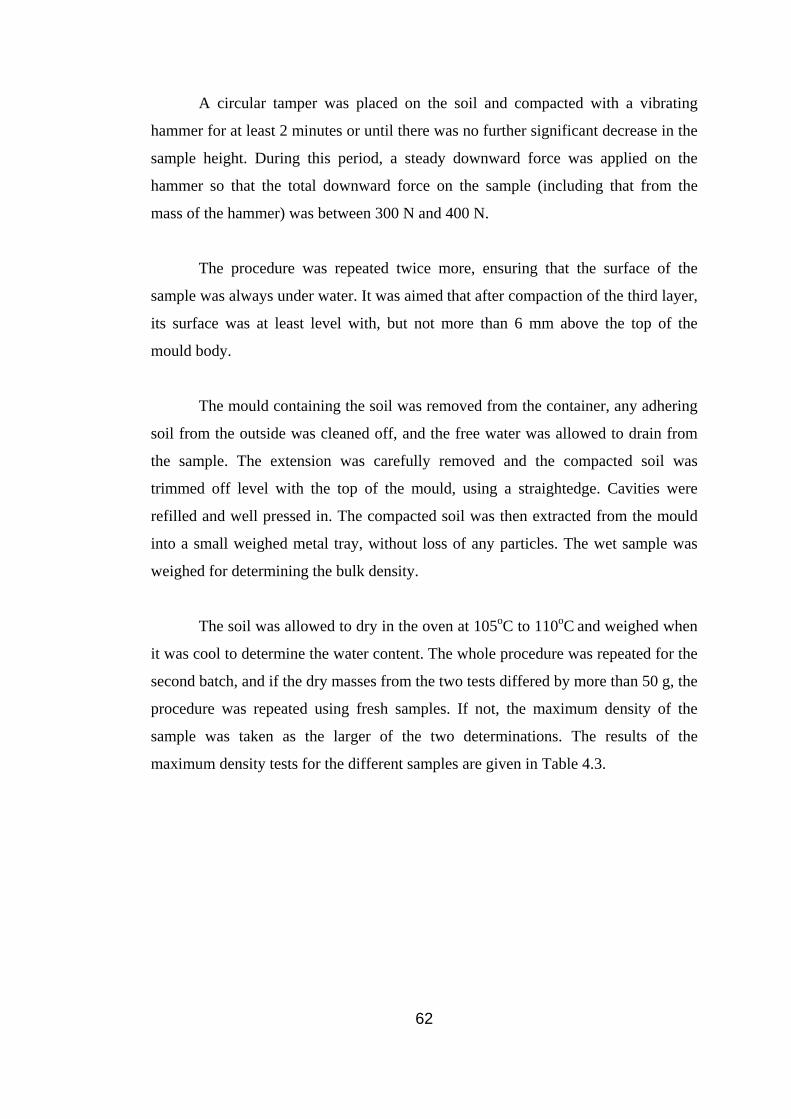
A circular tamper was placed on the soil and compacted with a vibrating
hammer for at least 2 minutes or until there was no further significant decrease in the
sample height. During this period, a steady downward force was applied on the
hammer so that the total downward force on the sample (including that from the
mass of the hammer) was between 300 N and 400 N.
The procedure was repeated twice more, ensuring that the surface of the
sample was always under water. It was aimed that after compaction of the third layer,
its surface was at least level with, but not more than 6 mm above the top of the
mould body.
The mould containing the soil was removed from the container, any adhering
soil from the outside was cleaned off, and the free water was allowed to drain from
the sample. The extension was carefully removed and the compacted soil was
trimmed off level with the top of the mould, using a straightedge. Cavities were
refilled and well pressed in. The compacted soil was then extracted from the mould
into a small weighed metal tray, without loss of any particles. The wet sample was
weighed for determining the bulk density.
The soil was allowed to dry in the oven at 105oC to 110oC and weighed when
it was cool to determine the water content. The whole procedure was repeated for the
second batch, and if the dry masses from the two tests differed by more than 50 g, the
procedure was repeated using fresh samples. If not, the maximum density of the
sample was taken as the larger of the two determinations. The results of the
maximum density tests for the different samples are given in Table 4.3.
62
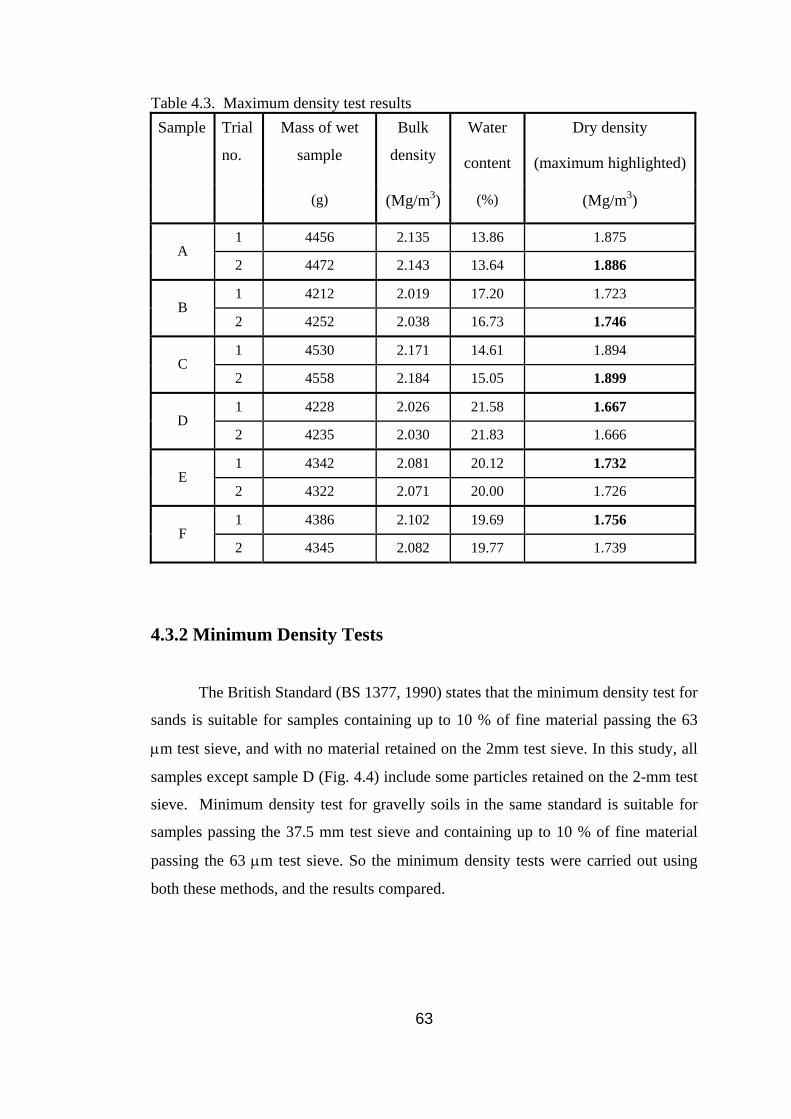
Table 4.3. Maximum density test results Mass of wet
sample
Bulk
density
Water
content
Dry density
(maximum highlighted)
Sample Trial
no.
(g) (Mg/m3) (%) (Mg/m3)
1 4456 2.135 13.86 1.875 A
2 4472 2.143 13.64 1.886
1 4212 2.019 17.20 1.723 B
2 4252 2.038 16.73 1.746
1 4530 2.171 14.61 1.894 C
2 4558 2.184 15.05 1.899
1 4228 2.026 21.58 1.667 D
2 4235 2.030 21.83 1.666
1 4342 2.081 20.12 1.732 E
2 4322 2.071 20.00 1.726
1 4386 2.102 19.69 1.756 F
2 4345 2.082 19.77 1.739
4.3.2 Minimum Density Tests
The British Standard (BS 1377, 1990) states that the minimum density test for
sands is suitable for samples containing up to 10 % of fine material passing the 63
µm test sieve, and with no material retained on the 2mm test sieve. In this study, all
samples except sample D (Fig. 4.4) include some particles retained on the 2-mm test
sieve. Minimum density test for gravelly soils in the same standard is suitable for
samples passing the 37.5 mm test sieve and containing up to 10 % of fine material
passing the 63 µm test sieve. So the minimum density tests were carried out using
both these methods, and the results compared.
63

4.3.2.1 Minimum Density Tests Performed by Following the
Procedure for Sands
A representative sample of 1 kg prepared as in section 3.2 was placed in a
1000 cm3 glass cylinder without a pouring lip, and a piece of rubber membrane was
held against the mouth of the cylinder. The cylinder was shaken to loosen the sand
and inverted a few times. During the last inversion, the cylinder was turned upside
down, and held until all the sample was at rest; then it was quickly turned the right
way up. The cylinder was put on a flat surface without jarring it. The volume reading
at the mean level of the surface of the sand was recorded to the nearest 10 cm3.
During this operation shaking or jolting the cylinder was avoided. The procedure was
repeated to give at least 10 determinations altogether. The minimum dry density
(ρd)min of the different samples was calculated as set out in Tables 4.4 and 4.5.
Table 4.4. Volume of specimen in the glass cylinder for different trials
Volume of specimen for ten different trials
(maximum highlighted)
(cm3)
Sample
1 2 3 4 5 6 7 8 9 10
A 610 620 610 620 620 620 620 620 610 620
B 710 710 700 700 710 710 710 700 710 710
C 580 600 590 580 570 580 600 580 580 600
D 670 670 680 680 670 670 670 680 680 680
E 660 660 670 670 670 660 670 660 660 670
F 670 660 670 660 660 670 670 670 670 670
64

Table 4.5. Calculation of minimum density from the procedure for sands
1 2 3 4 5 6
Mass of specimen
Maximum volume of specimen (cm3)
(from Table 4.4)
Bulk density
ρbulk
Air-dry
water content
(ρd)minSample
(g) (Mg/m3) (%) (Mg/m3)
A 620 1.613 0.850 1.599
B 710 1.408 0.179 1.406
C 600 1.667 0.336 1.661
D 680 1.471 0.135 1.469
E 670 1.492 0.208 1.489
F
1000
670 1.492 0.472 1.485
4.3.2.2 Minimum Density Tests Performed by Following the
Procedure for Gravelly Soils
The sample prepared as in section 3.2 was mixed thoroughly on a large tray,
and a representative sample of about 5 kg was obtained by riffling. The sample was
placed in a bucket and mixed to ensure an even distribution of particles of all sizes.
The CBR mould, 152 mm in diameter and 115 mm high, with base and extension
attached, was then placed in a tray and the contents of the bucket was poured into the
mould steadily from a height of about 50 cm by using a hand-scoop. The extension
was carefully removed and the surface of the soil was leveled to the top of the mould
using a straightedge without disturbing the soil in the mould or jarring the mould.
The weight of soil in the mould was determined; this soil was then remixed
with the excess soil remaining on the tray. The procedure was repeated to give at
least 10 determinations altogether. The minimum density of the different samples
was calculated as set out in Tables 4.6 and 4.7.
65
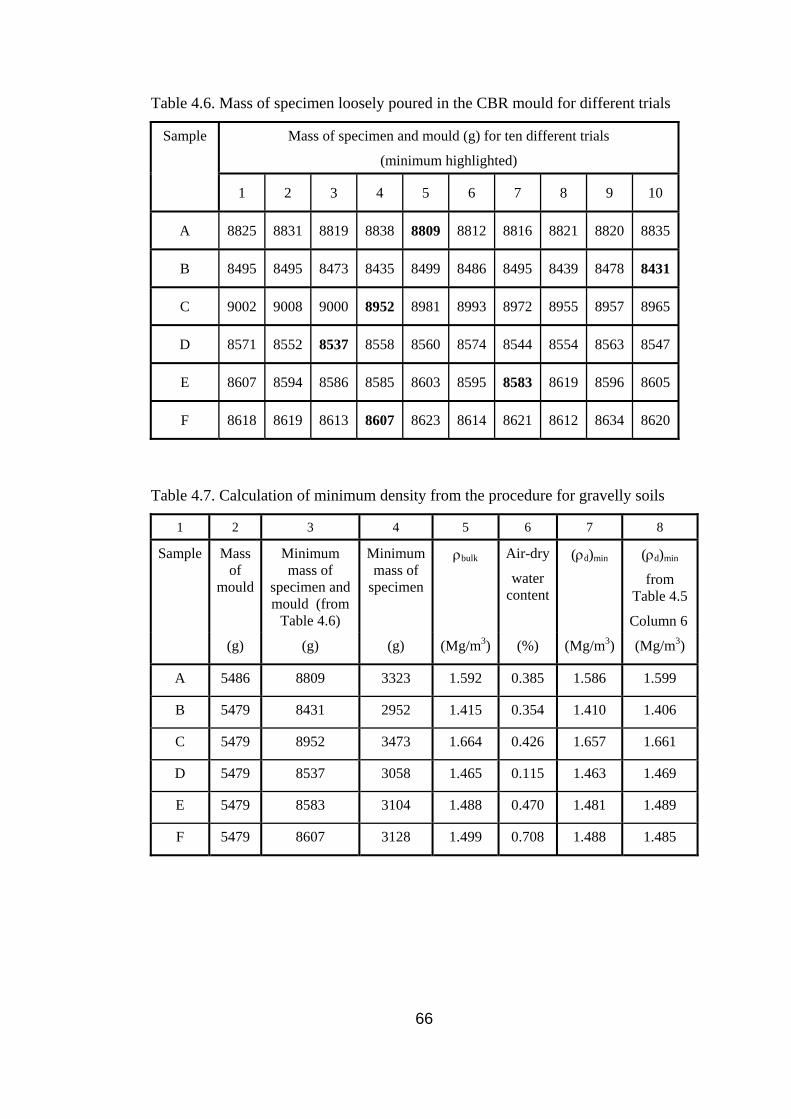
Table 4.6. Mass of specimen loosely poured in the CBR mould for different trials
Mass of specimen and mould (g) for ten different trials
(minimum highlighted)
Sample
1 2 3 4 5 6 7 8 9 10
A 8825 8831 8819 8838 8809 8812 8816 8821 8820 8835
B 8495 8495 8473 8435 8499 8486 8495 8439 8478 8431
C 9002 9008 9000 8952 8981 8993 8972 8955 8957 8965
D 8571 8552 8537 8558 8560 8574 8544 8554 8563 8547
E 8607 8594 8586 8585 8603 8595 8583 8619 8596 8605
F 8618 8619 8613 8607 8623 8614 8621 8612 8634 8620
Table 4.7. Calculation of minimum density from the procedure for gravelly soils
1 2 3 4 5 6 7 8
Sample Mass of
mould
Minimum mass of
specimen and mould (from
Table 4.6)
Minimum mass of
specimen
ρbulk
Air-dry
water content
(ρd)min
(ρd)min
from Table 4.5
Column 6
(g) (g) (g) (Mg/m3) (%) (Mg/m3) (Mg/m3)
A 5486 8809 3323 1.592 0.385 1.586 1.599
B 5479 8431 2952 1.415 0.354 1.410 1.406
C 5479 8952 3473 1.664 0.426 1.657 1.661
D 5479 8537 3058 1.465 0.115 1.463 1.469
E 5479 8583 3104 1.488 0.470 1.481 1.489
F 5479 8607 3128 1.499 0.708 1.488 1.485
66
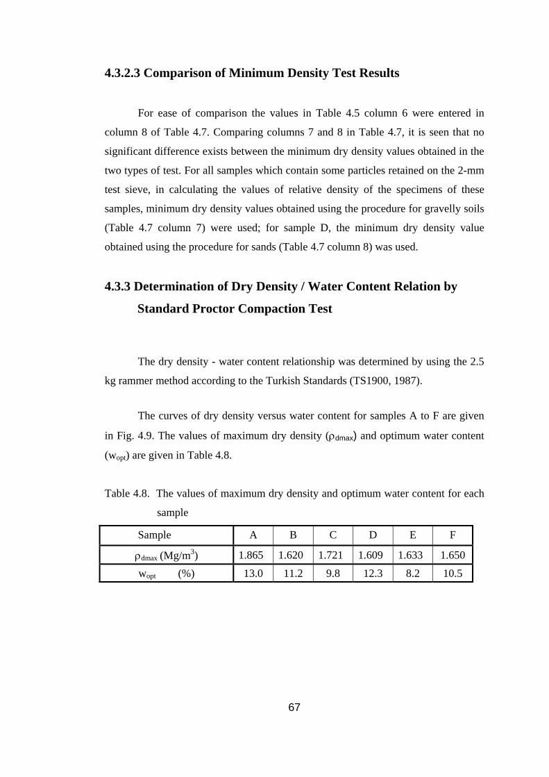
4.3.2.3 Comparison of Minimum Density Test Results
For ease of comparison the values in Table 4.5 column 6 were entered in
column 8 of Table 4.7. Comparing columns 7 and 8 in Table 4.7, it is seen that no
significant difference exists between the minimum dry density values obtained in the
two types of test. For all samples which contain some particles retained on the 2-mm
test sieve, in calculating the values of relative density of the specimens of these
samples, minimum dry density values obtained using the procedure for gravelly soils
(Table 4.7 column 7) were used; for sample D, the minimum dry density value
obtained using the procedure for sands (Table 4.7 column 8) was used.
4.3.3 Determination of Dry Density / Water Content Relation by
Standard Proctor Compaction Test
The dry density - water content relationship was determined by using the 2.5
kg rammer method according to the Turkish Standards (TS1900, 1987).
The curves of dry density versus water content for samples A to F are given
in Fig. 4.9. The values of maximum dry density (ρdmax) and optimum water content
(wopt) are given in Table 4.8.
Table 4.8. The values of maximum dry density and optimum water content for each
sample
Sample A B C D E F
ρdmax (Mg/m3) 1.865 1.620 1.721 1.609 1.633 1.650
wopt (%) 13.0 11.2 9.8 12.3 8.2 10.5
67

4 8 12 16 20 24Water content (%)
1.70
1.75
1.80
1.85
1.90
Dry
den
sity
4 8 12 16Water content (%)
1.56
1.58
1.60
1.62
1.64
Dry
de
2 4 6 8 10 12 1Water content (%)
4 4 8 12 16Water content (%)
1.58
1.59
1.60
1.61
1.62
Dry
den
sity
4 6 8 10 12 14 6 8 10 12 14Water content (%)
1.60
1.62
1.64
1.66
Dry
den
sity
nsity
(Mg/
m3 )
(Mg/
m3 )
Sample A Sample B
1.66
1.68
1.70
1.72
1.74
Dry
den
sity
(Mg/
m3 )
(Mg/
m3 )
Sample C Sample D
Water content (%)
1.62
1.63
1.64
Dry
den
sity
(Mg/
m3 )
(Mg/
m3 )
Sample F Sample E
Figure 4.9. The compaction curves for samples A to F
68
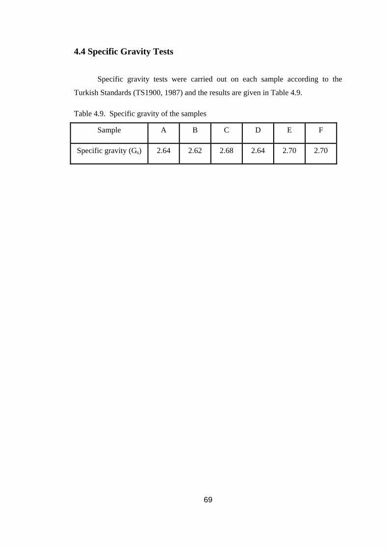
4.4 Specific Gravity Tests
Specific gravity tests were carried out on each sample according to the
Turkish Standards (TS1900, 1987) and the results are given in Table 4.9. Table 4.9. Specific gravity of the samples
Sample A B C D E F
Specific gravity (Gs) 2.64 2.62 2.68 2.64 2.70 2.70
69

CHAPTER 5
WEDGE SHEAR TESTS PERFORMED
5.1 Cylindrical Wedge Shear Tests Performed
5.1.1 Introduction
Cylindrical wedge shear tests (cylwests) have been carried out using an
available compression machine (Fig. 5.1(a)) modified as explained in section 5.1.3,
and a double-cut cylwest mould with both cuts inclined at 30o to the axis (Fig 5.1(b)).
5.1.2 Calculation of Wet Mass of Each Layer
To obtain the same degree of compaction as in the standard Proctor test, the
wet mass of each layer and the number of layers in the cylwest mould were
calculated to give the same compacted height per layer and the same compactive
effort per unit volume as in the standard Proctor test as follows.
In the standard Proctor test, average compacted height per layer is 4 cm and
the inside diameter of the mould is 10.16 cm, giving a volume of 324.28 cm3. When
the sand is compacted in the cylwest mould, whose inside diameter is 10.44 cm,
using the same height per layer,
Compacted volume /layer = 324.28 x 244.10 ⎞
16.10⎟⎠
⎜⎝⎛ = 342.40 cm3
70
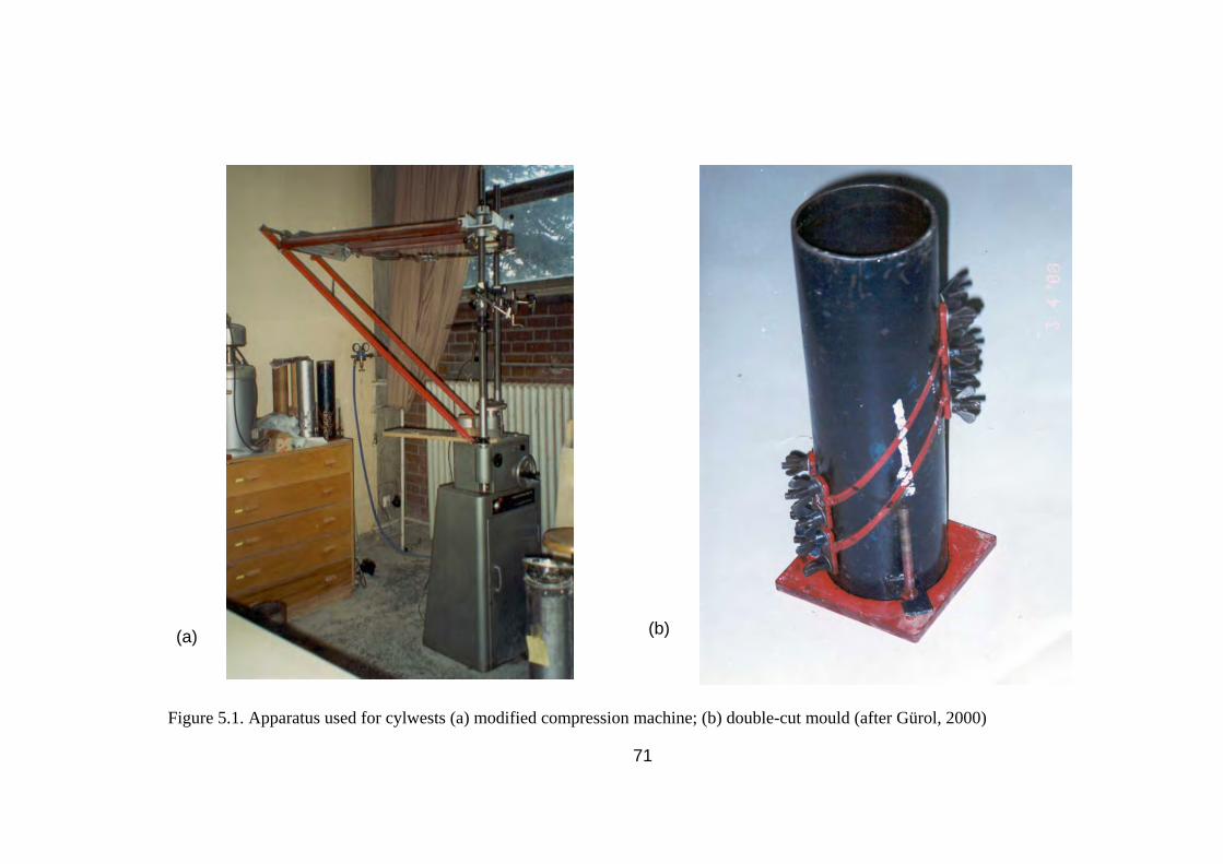
71
Figure 5.1. Apparatus used for cylwests (a) modified compression machine; (b) double-cut mould (after Gürol, 2000)
(a) (b)

The wet mass of each layer to be compacted to a height of 40 mm in the cylwest
mould = 342.40 x ρbulk
The bulk density ρbulk was calculated from
ρbulk = ρdmax (1+wopt )
where ρdmax and wopt for each sample are given in Table 4.8.
To ensure that the top of the sample was well above the upper cut of the
mould (Fig. 5.2), the sample was compacted in 9 layers of 40 mm each, giving a total
height of 382 mm including the 22 mm high disc at the bottom.
5.1.3 Test Procedure
The following paragraphs have been mostly quoted from Gürol (2000), based
on Gün (1997) and Mirata (1991).
1. A tightly fitting wooden disc of 22 mm thickness was inserted in the
bottom of the cylwest mould to prevent the cohesionless material from falling out of
the mould during handling. The mould was secured on the base plate. For each
sample prepared for cylwests as in section 3.2, the calculated amount of sand per
layer (section 5.1.2) was weighed, placed in the mould and compacted by using the
2.5 kg rammer to obtain a lower density, and by using the Kango vibrating hammer
to obtain a higher density. This procedure was repeated for eight more layers. The
specimen compacted in the mould was weighed, the height of the empty portion
above the specimen was measured in order to provide the same bulk density in the
subsequent shear tests on the same sample, and wooden discs of appropriate height
were placed in the empty portion such that they would be flush with the top of the
mould.
72
2. A 5-ton, electrically loaded compression machine was used for loading. To
enable the use of this machine for cylwests without impairing its original
construction, the cross-beam was replaced by a channel CH as described by Mirata
(1991), and the supports for the lateral loading devices mounted on lugs L welded on
to the channel CH (Fig. 5.3(a)), and hinged clamps HC; another pair of hinged
clamps HC were used to fix the temporary support TS in position on one of the strain
rods SR of the compression machine (Fig. 5.3(b)); and a hook HK was welded on to
CH for supporting the yoke Y when not in use. Full details of these attachments are
given by Mirata (2003(a)). The loading rate was adjusted to 0.15 mm/min and 0.06
mm/min for the samples at the lower and higher densities respectively.
3. The cylwest mould was inserted between the jaws of the clamp C attached
to the channel CH, and supported temporarily by the hooked lugs HL (Fig. 5.2(a))
using the rotatable bar TS (Fig. 5.3(b)). The proving ring was set to zero with the
grooved plates LP1 and LP2, with the ball cage BC in between, mounted on top.
This unit was then placed on the single ball SB resting in a central recess on a steel
plate on the loading platen of the compression machine; the test mould was placed
on top of LP1, and the loading platen raised until the mould just touched the channel
CH (Fig. 5.3(a)). The mould was clamped on to this channel, tightening the vertical
screws on the clamp lightly first, then tightening the horizontal screws evenly, and
finally tightening the vertical screws. A small load of about 100 N was then applied.
4. The lateral force Q was applied by means of the yoke Y attached to the
turnbuckle T and the 900 N capacity spring balance SB (Fig. 5.3(a)). During
assembly of the equipment, the yoke rested in the dashed position held by the hook
HK. To apply Q, the yoke was swung around to the lower position, and Q was
adjusted to the desired value. Q was then kept constant until the peak strength was
reached. As relatively large values of Q were to be applied, the rigidity of the
stationary part TM (S) of the mould was improved by inserting a cross-bar CB and
suitable packing between its lower tip and the strain rods SR (Fig. 5.3(c)).
73
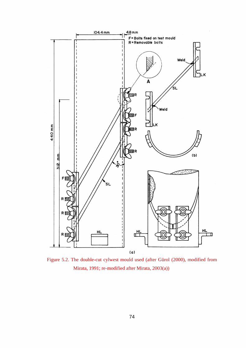
Figure 5.2. The double-cut cylwest mould used (after Gürol (2000), modified from
Mirata, 1991; re-modified after Mirata, 2003(a))
74

Figure 5.3. Layout for cylwests performed using a 5-ton compression machine
(after Gün, 1997)
75

5. Two dial gauges were mounted in position for measuring the
displacements of the mould in the direction of the main load P and perpendicular to
this direction; for recording the slight rotation β of the mould during the test,
another dial gauge was set to register the relative displacement between the grooved
plates.
6. As the sand was unable to hold itself in the stationary part of the mould
TM (S) after the test, only one test could be performed on the sample after each
compaction. So the upper cut of the mould was used in all tests, as this imposed
lower moments on the clamp C during application of Q. The screws securing the
upper pair of mould couplings (Fig. 5.2) were removed and the average clearance nc
between the shearing planes of the two halves of the mould was determined.
7. The catches and brackets on LP1 were turned free of LP2, and the two
grooved plates aligned by shifting the single ball. No initial eccentricity was applied.
The initial readings of the proving ring dial, and the three displacement dials were
recorded.
8. The specimen was sheared by increasing the axial load P. After the peak
strength was reached, the test was prolonged to measure the ultimate strength. At this
stage, calculator programs given by Mirata (2003(a)) were used to adjust Q to keep
σ at about its value at peak strength. The test was continued until ultimate strength
was reached (see Appendix D).
9. The dial gauges were removed. The two grooved plates were fastened
together using the swivel catches and brackets. Then Q was decreased to about 100
N, and the yoke stretched and hung on to the hook HK (Fig. 5.3(a)). The vertical
screws holding one jaw of the clamp were slackened. The horizontal screws of the
clamp were slackened evenly. The mould was rotated until it could be supported by
means of the rotatable bar TS (Fig. 5.3(b)) through one of the lugs. The loading
platen was lowered. The proving ring and the attached grooved plates were
76

removed, and placed on a plate with a central recess. Holding its two parts together,
the mould was removed.
10. The tested specimen was extracted from the test mould and the water
content was checked.
11. The same specimen was re-compacted in the cylwest mould as in step 1.
Steps 2 to 10 were then repeated using a higher lateral load Q.
12. Steps 1 to 11 were repeated on one more specimen of the same sample
prepared as in section 3.2.
Each cylwest, including specimen preparation, took about 1.5 hours.
5.1.4 Order of Testing Cylwest Specimens
In accordance with steps (11) and (12) of the test procedure (section 5.1.3),
the order of testing of the specimens is summarized below.
In the cylwests at the lower density, the order of testing given in the
following paragraph and summarized in Table 5.1, columns 2 to 5 was applied on all
samples.
An untested specimen was used for test 1 (column 2). The specimen used in
test 1 was recompacted and test 2 (column 3) was performed. Another untested
specimen was used for test 3 (column 4). The specimen used in test 3 was
recompacted and test 4 (column 5) was performed.
77

Table 5.1. Specimens used in the cylwests 1 2 3 4 5 6 7 8 9
Cylwests at the lower density Cylwests at the higher density
Sample Test 1
Q ≈ 93 N
Test 2
Q ≈ 436 N
Test 3
Q ≈ 93 N
Test 4
Q ≈ 436 N
Test 1
Q ≈ 110 N
Test 2
Q ≈ 436 N
Test 3
Q ≈ 110 N
Test 4
Q ≈ 436 N
A S.U. * R.A.T.**
(col. 2) S.U.
R.A.T.
(col. 4) … … … …
B S.U. R.A.T.
(col. 2) S.U.
R.A.T.
(col. 4) … … … …
C S.U. R.A.T.
(col. 2) S.U.
R.A.T.
(col. 4) … … … …
D S.U. R.A.T.
(col. 2) S.U.
R.A.T.
(col. 4) S.U.
R.A.T.
(col. 6) S.U.
R.A.T.
(col. 8)
E S.U. R.A.T.
(col. 2) S.U.
R.A.T.
(col. 4) S.U.
R.A.T.
(col. 6) S.U.
R.A.T.
(col. 8)
F S.U. R.A.T.
(col. 2) S.U.
R.A.T.
(col. 4) S.U.
R.A.T.
(col. 6) S.U.
R.A.T.
(col. 8)
* S.U.: separate untested specimen. * * R.A.T. (col. n): specimen reused after test in column n.
78
In the cylwests at the higher density, the order of testing given in the
following paragraph and summarized in Table 5.1, columns 6 to 9 was applied on
samples D to F. Samples A to C were not tested in cylwests at the higher density.
An untested specimen was used for test 1 (column 6). The specimen used in
test 1 was recompacted and test 2 (column 7) was performed. Another untested
specimen was compacted and test 3 (column 8) was performed. The specimen used
in test 3 was recompacted and test 4 (column 9) was performed.
5.1.5 Evaluation of Test Results
The tests were evaluated by using the computer program CYLWEE88
(Mirata, 2003(a)) which performs all three types of analysis explained by Mirata
(1991), and summarized in section 2.3.1. The results of cylwests presented are those
based on analysis C (section 2.3.1.4).
5.1.6 Test Results
Cylwest series CA to CF of four tests each were performed on samples A to F
respectively, at the lower density. The results obtained from the cylwest and triaxial
test series on samples A to F at the lower density had shown that the difference in the
measured φd values for samples A to C were higher than those for samples D to F
(Table 8.3, column (17)). An increase in density causes the difference in the
measured φd values in plane strain and triaxial tests to increase (section 2.1.4). To see
whether the difference in the measured φd values would increase with density,
additional three cylwest series CDH, CEH, and CFH of four tests each were
performed on samples D to F respectively, at the higher density.
The principal features of the cylwests are given in Tables 5.2 to 5.4. In these
tables, αn = nominal angle between the shear plane and the axis of test mould;
α = true angle between the shear plane and the axis of the test mould at peak
79
strength; nc = initial clearance between the stationary and the mobile halves of the
test mould; Dr = initial relative density, P = the main load applied; Q = lateral load;
u = average shear displacement; v = average normal displacement;
δσ/σ = percentage difference between the normal stress at the trailing end of the soil
wedge and the average normal stress; dv/du = rate of dilatation (change in v
(positive values indicating dilatation) divided by the change in u ). Figs. 5.4 and 5.5
show typical curves for series CA and CDH of the variation with u of shear stress τ,
u , dv/du, and β (Fig. 2.15).
It is observed from the u versus v curves (Figs. 5.4(b) and 5.5(b)) that at the
beginning of the tests, a drop in the v values has occurred, especially under the
higher values of Q; in the later stages of the tests, dilation has occurred. It is
observed from the u versus dv/du curves (Figs. 5.4(d) and 5.5(d)) that at the end of
the tests, the values of dv/du are nearly zero, showing that tests have been
sufficiently prolonged to yield the ultimate strength.
The results of cylwest series CA to CF and series CDH to CFH are plotted in
Figs. 5.6 and 5.7, and summarized in Tables 5.5 to 5.7. In these tables, e is the initial
void ratio; Dr is the initial relative density.
80

Table 5.2. Principal features of cylwest series CA to CC on samples A to C respectively.
1 2 3 4 5 6 7 8 9 10 11 12 13 14 15 16 17 18 19 Values at peak strength Values at ultimate strength αn
α
nc
Dr
P Q u v dv/du β δσ/σ P Q u v dv/du β δσ/σ
Test no.
(deg) (deg) (mm) (%) (N) (N) (mm) (mm) ratio (deg) (%) (N) (N) (mm) (mm) ratio (deg) (%)
CA/1 31.4 29.2 8.2 67.9 1705 100 3.1 0.95 0.55 -0.13 44.9 1326 585 5.9 0.44 -0.25 -0.06 11.9
CA/2 31.4 29.2 8.2 69.4 3201 436 3.9 -0.40 0.33 0.09 11.0 2436 753 6.1 0.06 0.17 0.20 1.0
CA/3 31.4 29.2 8.2 69.8 1662 94 2.3 0.27 0.45 0.10 24.1 1164 437 5.4 0.86 0.11 0.16 8.0
CA/4 31.4 29.2 8.2 67.5 3031 445 3.6 -0.27 0.41 0.09 10.7 2165 760 5.8 0.21 0.03 0.11 0.8
CB/1 31.4 29.2 8.2 61.6 815 89 3.0 1.41 0.46 0.27 28.1 731 336 10.1 1.56 0.02 0.53 -2.1
CB/2 31.4 29.2 8.2 62.7 1874 442 3.1 -0.32 0.28 0.13 5.7 1475 742 8.3 0.59 0.09 0.35 -8.6
CB/3 31.4 29.2 8.2 62.7 693 88 2.1 0.48 0.46 0.14 36.1 629 287 7.7 1.26 -0.06 0.26 11.8
CB/4 31.4 29.2 8.2 63.3 1989 442 3.1 0.01 0.27 0.18 4.1 1610 747 8.5 0.90 0.18 0.47 -11.5
CC/1 31.4 29.2 8.2 29.6 689 94 0.7 0.20 0.48 0.01 42.0 526 186 4.9 1.14 -0.10 0.28 23.3
CC/2 31.4 29.2 8.2 28.2 1763 436 2.5 -0.06 0.27 0.10 7.8 1382 612 9.5 0.53 -0.06 0.23 0.8
CC/3 31.4 29.2 8.2 25.7 650 94 1.0 0.40 0.54 0.06 41.4 488 181 8.3 1.39 0.01 0.44 20.2
CC/4 31.4 29.2 8.2 24.8 1826 436 3.1 -0.95 0.18 -0.15 19.8 1395 677 9.4 -0.31 0.00 0.22 -3.1
81

Table 5.3. Principal features of cylwest series CD to CF on samples D to F respectively.
1 2 3 4 5 6 7 8 9 10 11 12 13 14 15 16 17 18 19 Values at peak strength Values at ultimate strength αn
α
nc
Dr
P Q u v dv/du β δσ/σ P Q u v dv/du β δσ/σ
Test no.
(deg) (deg) (mm) (%) (N) (N) (mm) (mm) ratio (deg) (%) (N) (N) (mm) (mm) ratio (deg) (%)
CD/1 31.4 29.2 8.2 67.6 567 96 1.2 0.78 0.59 0.11 42.6 472 181 10.3 2.41 0.03 0.45 23.9
CD/2 31.4 29.2 8.2 65.7 1593 441 2.4 0.52 0.41 0.14 6.7 1272 624 7.8 1.27 0.01 0.12 4.2
CD/3 31.4 29.2 8.2 68.1 597 96 1.5 0.04 0.39 0.07 42.2 461 181 7.1 0.86 0.06 0.27 26.3
CD/4 31.4 29.2 8.2 68.1 1674 436 1.7 0.14 0.33 0.05 10.4 1271 667 7.9 0.68 0.03 0.43 -10.8
CE/1 31.4 29.2 8.2 65.5 843 102 2.5 0.56 0.31 0.10 34.3 595 238 8.2 0.15 0.01 0.36 11.0
CE/2 31.4 29.2 8.2 64.0 2226 440 3.0 0.27 0.30 -0.07 20.0 1531 741 10.2 0.19 -0.02 0.29 -5.6
CE/3 31.4 29.2 8.2 65.2 769 102 1.1 0.23 0.38 0.08 33.9 570 243 9.2 0.42 -0.02 0.53 2.7
CE/4 31.4 29.2 8.2 65.2 2309 441 2.5 0.05 0.31 0.11 8.5 1635 740 9.4 0.38 0.02 0.51 -10.3
CF/1 31.4 29.2 8.2 65.3 689 96 1.2 -0.15 0.55 -0.05 45.2 505 199 9.9 2.23 0.21 0.63 9.5
CF/2 31.4 29.2 8.2 65.0 1949 439 2.9 -0.27 0.20 0.11 7.7 1466 659 10.2 0.37 -0.04 0.03 7.3
CF/3 31.4 29.2 8.2 65.0 729 98 1.5 0.04 0.42 0.08 35.8 520 218 10.2 0.69 -0.01 0.57 3.7
CF/4 31.4 29.2 8.2 65.3 2056 441 2.8 0.01 0.20 0.10 9.1 1502 701 12.0 0.74 0.06 0.29 -2.8
82
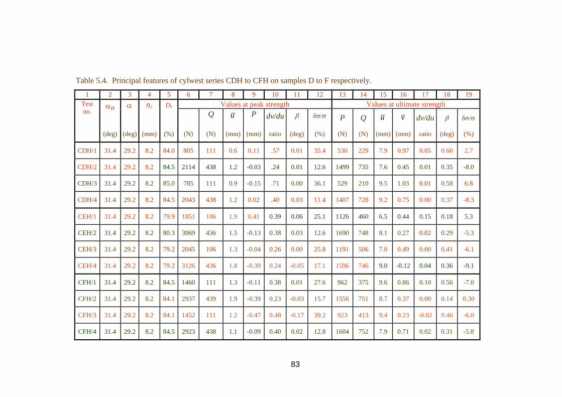
Table 5.4. Principal features of cylwest series CDH to CFH on samples D to F respectively.
83
1 2 3 4 5 6 7 8 9 10 11 12 13 14 15 16 17 18 19 Values at peak strength Values at ultimate strength αn
α
nc
Dr
Q u P dv/du β δσ/σ P Q u v dv/du β δσ/σ
Test no.
(deg) (deg) (mm) (%) (N) (N) (mm) (mm) ratio (deg) (%) (N) (N) (mm) (mm) ratio (deg) (%)
CDH/1 31.4 29.2 8.2 84.0 805 111 0.6 0.11 .57 0.01 35.4 530 229 7.9 0.97 0.05 0.60 2.7
CDH/2 31.4 29.2 8.2 84.5 2114 438 1.2 -0.03 .24 0.01 12.6 1499 735 7.6 0.45 0.01 0.35 -8.0
CDH/3 31.4 29.2 8.2 85.0 785 111 0.9 -0.15 .71 0.00 36.1 529 210 9.5 1.03 0.01 0.58 6.8
CDH/4 31.4 29.2 8.2 84.5 2043 438 1.2 0.02 .40 0.03 11.4 1407 728 9.2 0.75 0.00 0.37 -8.3
CEH/1 31.4 29.2 8.2 79.9 1851 106 1.9 0.41 0.39 0.06 25.1 1126 460 6.5 0.44 0.15 0.18 5.3
CEH/2 31.4 29.2 8.2 80.3 3069 436 1.5 -0.13 0.38 0.03 12.6 1690 748 8.1 0.27 0.02 0.29 -5.3
CEH/3 31.4 29.2 8.2 79.2 2045 106 1.3 -0.04 0.26 0.00 25.8 1191 506 7.0 0.49 0.00 0.41 -6.1
CEH/4 31.4 29.2 8.2 79.2 3126 436 1.8 -0.39 0.24 -0.05 17.1 1596 746 9.0 -0.12 0.04 0.36 -9.1
CFH/1 31.4 29.2 8.2 84.5 1460 111 1.3 -0.11 0.38 0.01 27.6 962 375 9.6 0.86 0.10 0.56 -7.0
CFH/2 31.4 29.2 8.2 84.1 2937 439 1.9 -0.39 0.23 -0.03 15.7 1556 751 8.7 0.37 0.00 0.14 0.30
CFH/3 31.4 29.2 8.2 84.1 1452 111 1.2 -0.47 0.48 -0.17 39.2 923 413 9.4 0.23 -0.02 0.46 -6.0
CFH/4 31.4 29.2 8.2 84.5 2923 438 1.1 -0.09 0.40 0.02 12.8 1604 752 7.9 0.71 0.02 0.31 -5.8

0 2 4 6 (mm)
80
100
200
(kPa
)
τ
0 2 4 6 8 u (mm)
-1
0
1
(m
m)
0 2 4 6 8 (mm)
-0.5
0 2 4 6 8 (mm)
-1
0
1
dv/d
u (ra
tio)
0.0
g
u v
(deg
)
0.5
(de
) β
Figure 5.4. Typical curves for series CA of the variation with of ( )a) τ, (b ,
(c) β, and (d) dv/du
υ CA/1 � CA/2
(b)
(c)
(d)
β
_
V
u (mm)
(mm)
u (mm)
u (mm)
dv/
du (r
atio
)
(a)
84
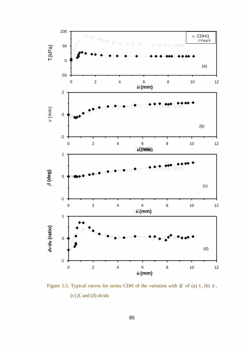
0 2 4 6 8 10 (mm)
12-50
0
50
100
0 2 4 6 8 10 (mm)
12-2
0
2
(m
m)
0 2 4 6 8 10 (mm)
12-1
0
1
(d
eg)
0 2 4 6 8 10 (mm)
12-1
0
1
dv/
du (r
atio
)
(c)
(d)
u u (mm)
(k
τ
Pa)
Figure 5.5. Typical curves for series CDH of the variation with u of (a) τ, (b) v
,
(c) β, and (d) dv/du
υ CDH/1 � CDH/2
(a)
(b)
β
u
u
(m
u (mm)
u (mm)
u (
mm)
mm)
dv/d
u (r
atio
)
β
(deg
)
u (
85

0 40 80 120 160Normal stress (kPa)
0
40
80
120
160
Shea
r stre
ngth
(kPa
)
0 30 60Normal stress (kPa)
900
30
60
90
Shea
r stre
ngth
(kPa
)
0 30 60 90
0 40 0 25 50 75 100Normal stress (kPa)
0
25
50
Normal stress (kPa)
0
30
60
Shea
r stre
ngth
(kPa
)
90 90 (c) Series CC (d) Series CD
0 30 60 90Normal stress (kPa)
0
30
60Sh
ear s
treng
th (k
Pa)
80 120Normal stress (kPa)
0
40
120
80Pa) 75
kPa)
100
Shea
r stre
ngth
(
Shea
r stre
ngth
(k
Figure 5.6. The results of cylwests on samples A to F at the lower density
(a) Series CA (b) Series CB
(e) Series CE (f) Series CF
υ υ at peak σ σ at ultimate
86
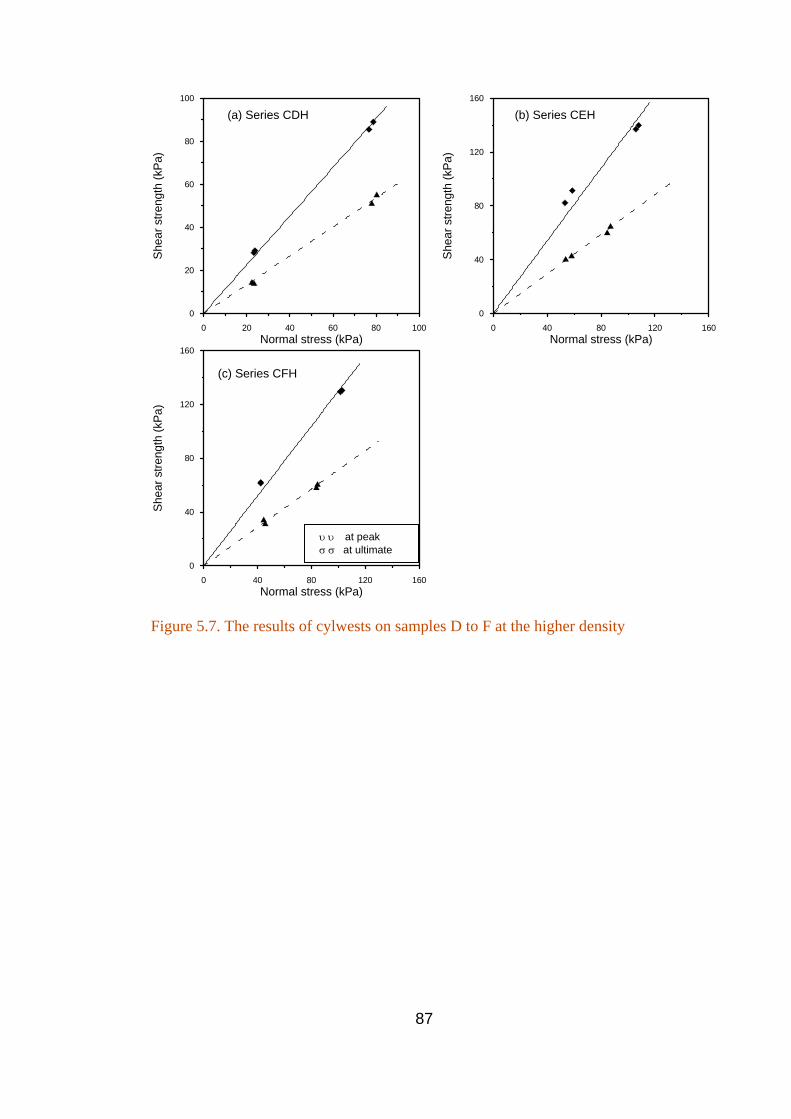
0 20 40 60 80 1Normal stress (kPa)
00
0 40 80 120 160Normal stress (kPa)
0
40
80
120
160
Shea
r stre
ngth
(kPa
)
Figure 5.7. The results of cylwests on samples D to F at the higher density
υ υ at peak σ σ at ultimate
(c) Series CFH
(a) Series CDH (b) Series CEH
0
20
40
60
80
100
Shea
r stre
ngth
0 40 80 120 160Normal stress (kPa)
0
40
80
120
160
Shea
r stre
ngth
(kPa
)
(kPa
)
87
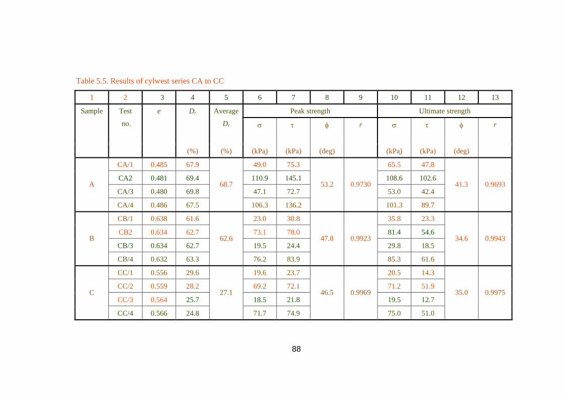
Table 5.5. Results of cylwest series CA to CC
1 2 3 4 5 6 7 8 9 10 11 12 13
Peak strength Ultimate strength Dr Average
Dr σ τ
φ r σ τ
φ r
Sample Test
no.
e
(%) (%) (kPa) (kPa) (deg) (kPa) (kPa) (deg)
CA/1 0.485 67.9 49.0 75.3 65.5 47.8
CA2 0.481 69.4 110.9 145.1 108.6 102.6
CA/3 0.480 69.8 47.1 72.7 53.0 42.4 A
CA/4 0.486 67.5
68.7
106.3 136.2
53.2 0.9730
101.3 89.7
41.3 0.9693
CB/1 0.638 61.6 23.0 30.8 35.8 23.3
CB2 0.634 62.7 73.1 78.0 81.4 54.6
CB/3 0.634 62.7 19.5 24.4 29.8 18.5 B
CB/4 0.632 63.3
62.6
76.2 83.9
47.8 0.9923
85.3 61.6
34.6 0.9943
CC/1 0.556 29.6 19.6 23.7 20.5 14.3
CC/2 0.559 28.2 69.2 72.1 71.2 51.9
CC/3 0.564 25.7 18.5 21.8 19.5 12.7 C
CC/4 0.566 24.8
27.1
71.7 74.9
46.5 0.9969
75.0 51.0
35.0 0.9975
88
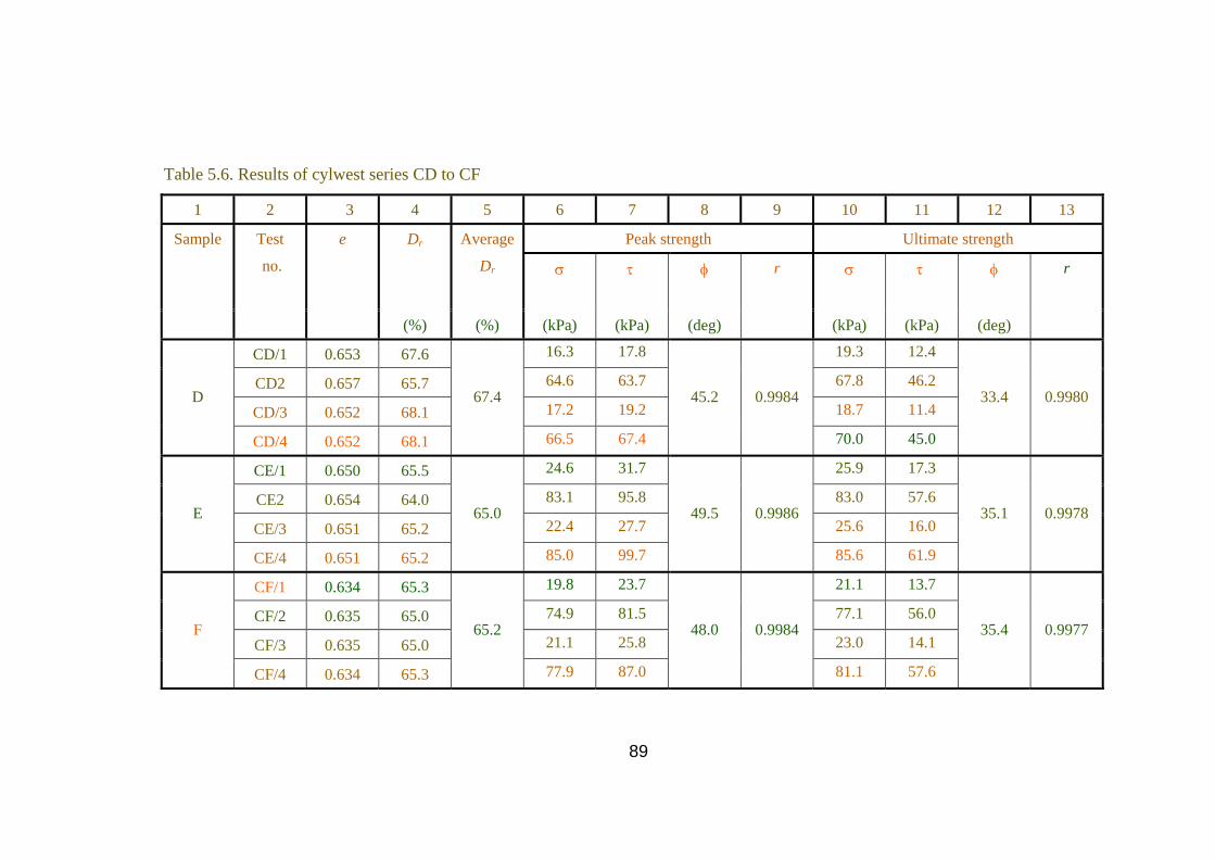
Table 5.6. Results of cylwest series CD to CF
1 2 3 4 5 6 7 8 9 10 11 12 13
Peak strength Ultimate strength Dr Average
Dr σ τ
φ r σ τ
φ r
Sample Test
no.
e
(%) (%) (kPa) (kPa) (deg) (kPa) (kPa) (deg)
CD/1 0.653 67.6 16.3 17.8 19.3 12.4
CD2 0.657 65.7 64.6 63.7 67.8 46.2
CD/3 0.652 68.1 17.2 19.2 18.7 11.4 D
CD/4 0.652 68.1
67.4
66.5 67.4
45.2 0.9984
70.0 45.0
33.4 0.9980
CE/1 0.650 65.5 24.6 31.7 25.9 17.3
CE2 0.654 64.0 83.1 95.8 83.0 57.6
CE/3 0.651 65.2 22.4 27.7 25.6 16.0 E
CE/4 0.651 65.2
65.0
85.0 99.7
49.5 0.9986
85.6 61.9
35.1 0.9978
CF/1 0.634 65.3 19.8 23.7 21.1 13.7
CF/2 0.635 65.0 74.9 81.5 77.1 56.0
CF/3 0.635 65.0 21.1 25.8 23.0 14.1 F
CF/4 0.634 65.3
65.2
77.9 87.0
48.0 0.9984
81.1 57.6
35.4 0.9977
89
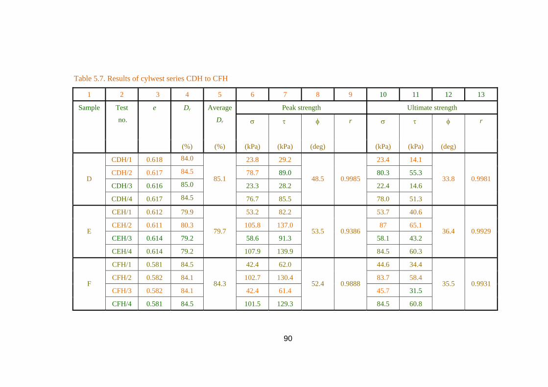
Table 5.7. Results of cylwest series CDH to CFH
1 2 3 4 5 6 7 8 9 10 11 12 13
Peak strength Ultimate strength Dr Average
Dr σ τ
φ r σ τ
φ r
Sample Test
no.
e
(%) (%) (kPa) (kPa) (deg) (kPa) (kPa) (deg)
CDH/1 0.618 84.0 23.8 29.2 23.4 14.1
CDH/2 0.617 84.5 78.7 89.0 80.3 55.3
CDH/3 0.616 85.0 23.3 28.2 22.4 14.6 D
CDH/4 0.617 84.5
85.1
76.7 85.5
48.5 0.9985
78.0 51.3
33.8 0.9981
CEH/1 0.612 79.9 53.2 82.2 53.7 40.6
CEH/2 0.611 80.3 105.8 137.0 87 65.1
CEH/3 0.614 79.2 58.6 91.3 58.1 43.2 E
CEH/4 0.614 79.2
79.7
107.9 139.9
53.5 0.9386
84.5 60.3
36.4 0.9929
CFH/1 0.581 84.5 42.4 62.0 44.6 34.4
CFH/2 0.582 84.1 102.7 130.4 83.7 58.4
CFH/3 0.582 84.1 42.4 61.4 45.7 31.5 F
CFH/4 0.581 84.5
84.3
101.5 129.3
52.4 0.9888
84.5 60.8
35.5 0.9931
90

5.1.7 Effect on the Cylwest Results of the Order of Testing In cylwests at the lower and higher densities, both of the untested specimens
had been sheared under the lower normal stress σ (Table 5.1). The effect on the
cylwest series CA (the plotted peak strength results of which show the largest
deviation from the fitted envelope in Fig. 5.6(a)) results of the order of testing can be
seen by examining Fig. 5.8. The test numbers are denoted on this figure.
0 40 80 120Normal stress (kPa)
1600
40
80
120
160
Shea
r stre
ngth
(kPa
)
2
4
1
3
- - - - __ _ __ F________
From tests 1 & 3 From tests 2 & 4
rom all four tests
Figure 5.8. The results of cylwest series CA
Fig. 5.8 shows that a higher peak friction angle φc2 would be obtained from
the two tests 1 and 3 than from tests 2 and 4. According to the sieve analysis before
and after cylwests, some particle crushing has occurred (Table 4.2). Crushing of sand
particles is considered as the main reason of the reduction in strength; also, an
increase in normal stress causes a reduction in strength (section 2.1.3). So, the φc2
value defined by tests 2 and 4 in Fig. 5.8 being smaller than that defined by tests 1
and 3 is an expected result. Had test 2, under the higher σ, been performed on an
91
untested specimen, the corresponding shear strength would be higher than shown in
Fig. 5.8; test 3 then would have to be performed on a re-sheared specimen, resulting
in a lower shear strength than shown in Fig. 5.8. The net result of this altered order of
testing would probably be a relatively small increase in the φ value defined by the
full line in Fig. 5.8.
5.2 Prismatic Wedge Shear Tests Performed
5.2.1 Introduction
The prismatic wedge shear tests (priswests) have been carried out using a
20-ton loading frame (Mirata, 1992; 2003(a)) and two different test moulds whose
shearing planes were inclined at angles αn = 30o and 40o to the main load. In this
section, the description of the priswest apparatus, the test procedure, the order of
testing priswest specimens, and the results of the tests are presented. Sections 5.2.2
and 5.2.3 have been adapted from Mirata (1991,1992, 2003(a)).
5.2.2 Description of the Priswest Apparatus
The apparatus used in this study is a portable system consisting of loading
devices, a test mould and a 20-ton capacity version of the simple, 5-ton frame shown
in Fig. 5.9. The modifications to this frame to convert it into a 20-ton one is shown
in Fig. 5.10. The priswest mould is made of 10-mm thick mild steel plate, and
consists of two identical halves, each with a shear plane measuring 300 mm x 300
mm internally. The mobile half TM has a removable lid; the stationary half TM (S) is
bolted on the left - hand beam of the frame (Fig. 5.9(b)). Initially, the two halves of
the mould are bolted together through four pairs of links with spacers SR screwed in
the middle, and the lid on TM is replaced by a 70 - mm high collar (Fig. 5.9(a)) while
the sample is placed in the mould. The grooved loading plates LP1 and LP2, the ball
92
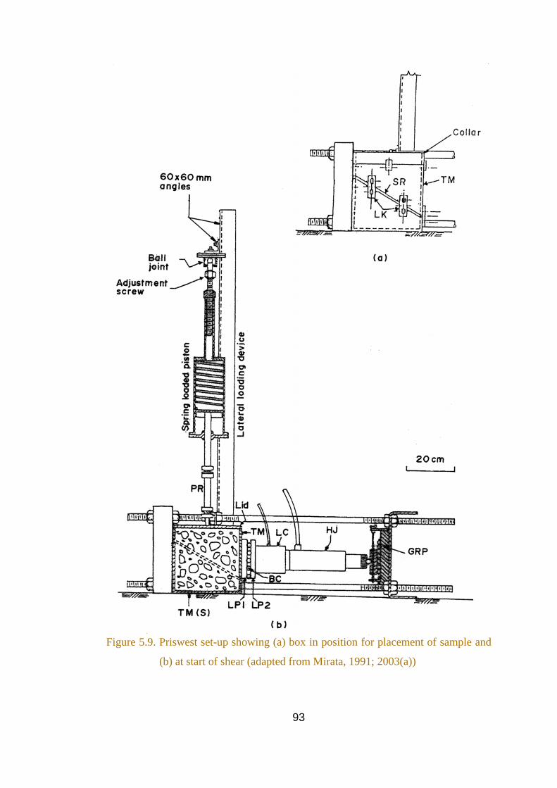
Figure 5.9. Priswest set-up showing (a) box in position for placement of sample and
(b) at start of shear (adapted from Mirata, 1991; 2003(a))
93

cage BC, the load cell LC, and the hydraulic jack HJ are placed between the grooved
reaction plate GRP and the test mould TM (Fig. 5.9(b)). The lateral loading device
consists of a spring loaded piston, or preferably an air piston as used in this study.
Figure 5.10. Modified cross – beam of 20 ton priswest frame (after Mirata, 1992)
94
5.2.3 Test Procedure
1. To facilitate the various operations, the lateral loading device (Fig. 5.9(b))
was removed. The lid on TM (Fig. 5.9(b)) was removed, and to prevent grit blocking
the tapped holes at the top of the mould, these were temporarily covered with sticky
tape. The collar (Fig. 5.9(a)) was screwed on top of the mould through the four lugs.
2. For each sample prepared as in section 3.2, the amount of sand per layer of
thickness one-fifth of the total depth of the mould plus 2 mm, required to give the
same wet density as that obtained in cylwests was calculated. This amount was
compacted to the desired thickness in the priswest mould by applying vibration,
using the Kango hammer, directly on the sand for 90 seconds and on a 10-mm thick
steel plate placed on top of the sand for another 30 seconds. This procedure was
repeated five times, obtaining a compacted sample with the top about 10 mm above
the top of the mould.
3. The collar was then removed, the surplus material scraped off, and the
surface smoothed. The temporary tapes were removed, and the lid secured in position
by fly-bolts. The lateral loading device carrying a proving ring was mounted in
position; the proving dial was set to zero before the tip contacted the test mould, and a lateral load of about 150 N was applied.
4. The grooved loading plates LP1 and LP2, the ball cage BC, the load cell
LC, and the hydraulic jack HJ were placed between the grooved reaction plate GRP
and the test mould TM (Figure 5.9(b)). A main load P of about 200 N was applied.
5. The spacers were removed. Dial gauges were mounted in position for
measuring the displacements of the mould in the direction of P and perpendicular to
this direction; for recording the slight rotation of the mould during the test, another
dial gauge was set to register the relative displacement between the grooved plates.
95

6. The lateral load Q was raised gradually to the desired value, increasing P
by about equal increments. Keeping Q constant, P was gradually increased producing
a displacement rate of about 0.5 mm/min in the direction of P. Readings of the
displacement dials, and of P and Q were taken. Loading was continued until P
started dropping. Then Q was adjusted approximately as explained by Mirata
(2003(a)) to keep the normal stress σ at about its value at peak strength; in this
approximate method, Q is increased to keep P close to but somewhat below its value
at peak strength to account for the reduction in the shear plane area, and the
relatively small contribution of Q to σ. At this stage, the rate of loading was
increased between readings, restoring this rate to the original value during the
readings to minimize rheological effects.
7. At the end of the test, the dial gauges were first removed; Q was then
reduced to zero; the lateral loading device was removed. Taking care of the load cell
and the grooved plates, P was reduced to zero. The grooved plates, the ball cage, and
the load cell were removed. The load cell was stored in a safe place. The grooved
plates and ball cage were stored in a dust-proof container. A moisture content
specimen was taken from the failure plane; the mould was emptied, cleaned and
smeared with machine oil to minimize oxidation.
Each priswest, including specimen preparation, took about 2 hours.
5.2.4 Order of Testing Priswest Specimens
In the priswests on specimens at the lower density, the order of testing given
in the following two paragraphs and summarized in Table 5.8, columns 2 to 7 was
applied for the different samples.
96
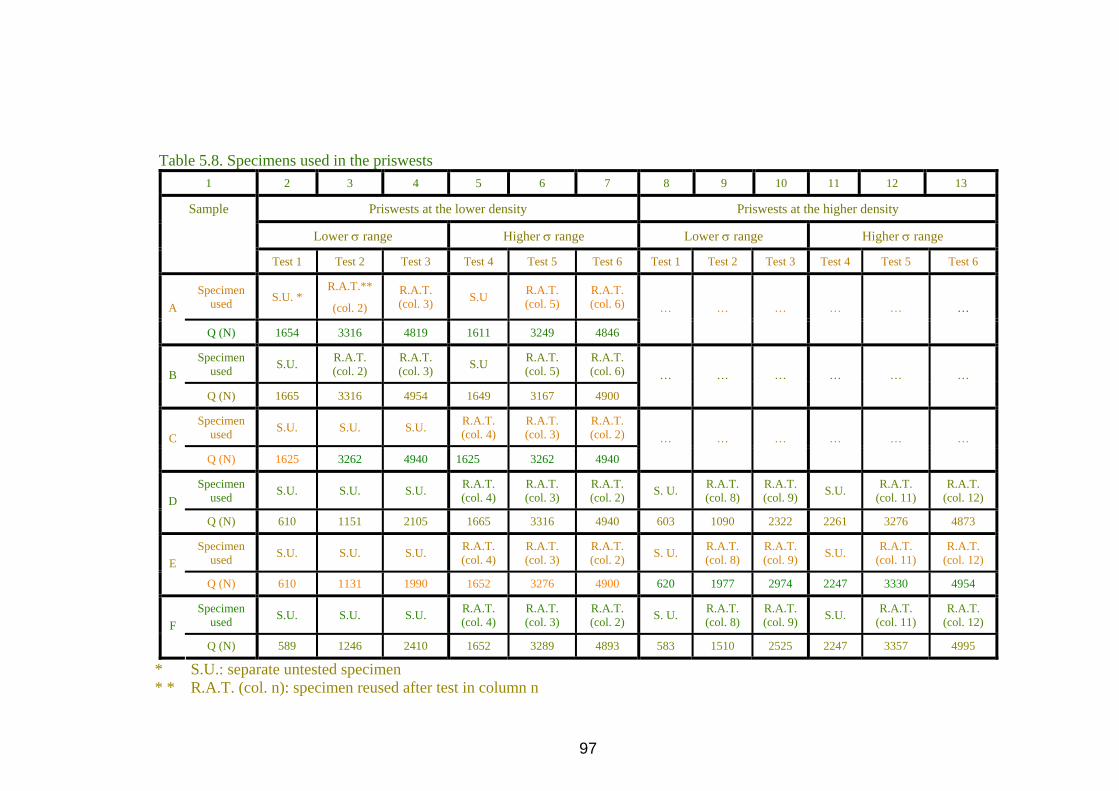
Table 5.8. Specimens used in the priswests 1 2 3 4 5 6 7 8 9 10 11 12 13
Priswests at the lower density Priswests at the higher density
Lower σ range Higher σ range Lower σ range Higher σ range
Sample
Test 1 Test 2 Test 3 Test 4 Test 5 Test 6 Test 1 Test 2 Test 3 Test 4 Test 5 Test 6
Specimen used S.U. *
R.A.T.**
(col. 2) R.A.T. (col. 3) S.U R.A.T.
(col. 5) R.A.T. (col. 6) A
Q (N) 1654 3316 4819 1611 3249 4846
… … … … … …
Specimen used S.U. R.A.T.
(col. 2) R.A.T. (col. 3) S.U R.A.T.
(col. 5) R.A.T. (col. 6) B
Q (N) 1665 3316 4954 1649 3167 4900
… … … … … …
Specimen used S.U. S.U. S.U. R.A.T.
(col. 4) R.A.T. (col. 3)
R.A.T. (col. 2) C
Q (N) 1625 3262 4940 1625 3262 4940
… … … … … …
Specimen used S.U. S.U. S.U. R.A.T.
(col. 4) R.A.T. (col. 3)
R.A.T. (col. 2) S. U. R.A.T.
(col. 8) R.A.T. (col. 9) S.U. R.A.T.
(col. 11) R.A.T.
(col. 12) D
Q (N) 610 1151 2105 1665 3316 4940 603 1090 2322 2261 3276 4873
Specimen used S.U. S.U. S.U. R.A.T.
(col. 4) R.A.T. (col. 3)
R.A.T. (col. 2) S. U. R.A.T.
(col. 8) R.A.T. (col. 9) S.U. R.A.T.
(col. 11) R.A.T.
(col. 12) E
Q (N) 610 1131 1990 1652 3276 4900 620 1977 2974 2247 3330 4954
Specimen used S.U. S.U. S.U. R.A.T.
(col. 4) R.A.T. (col. 3)
R.A.T. (col. 2) S. U. R.A.T.
(col. 8) R.A.T. (col. 9) S.U. R.A.T.
(col. 11) R.A.T.
(col. 12) F
Q (N) 589 1246 2410 1652 3289 4893 583 1510 2525 2247 3357 4995
* S.U.: separate untested specimen * * R.A.T. (col. n): specimen reused after test in column n
97
For each of the samples A and B, an untested specimen was used for test 1
(column 2). The specimen used in test 1 was recompacted and test 2 (column 3) was
performed. The specimen used in test 2 was compacted a third time and test 3
(column 4) was performed. Another untested specimen was used for test 4 (column
5). The specimen used in test 4 was recompacted and test 5 (column 6) was
performed. The specimen used in test 5 was compacted a third time and test 6
(column 7) was performed.
For each of the samples C to F, each of the tests under the lower σ (columns
2 to 4) was performed on a separate untested specimen. Each specimen used in tests
3, 2, and 1 was recompacted, and test 4 (column 5), test 5 (column 6), and test 6
(column 7) respectively were performed.
In the priswests on specimens at the higher density, the order of testing given
in the following paragraph and summarized in Table 5.8, columns 8 to 13 was
applied on samples D to F. Samples A to C were not tested at the higher density.
For each of the samples D to F, an untested specimen was used for test 1
(column 8). The specimen used in test 1 was recompacted and test 2 (column 9) was
performed. The specimen used in test 2 was compacted a third time and test 3
(column 10) was performed. Another untested specimen was compacted and test 4
(column 11) was performed. The specimen used in test 4 was recompacted and test 5
(column 12) was performed. The specimen used in test 5 was compacted a third time
and test 6 (column 13) was performed.
5.2.5 Evaluation of the Test Results
The tests were evaluated by using the computer program IWPW77
(Mirata, 2003(a)) which performs all three types of analysis explained by Mirata
(1991), and summarized in section 2.3.1. The results of priswests presented are those
based on analysis C (section 2.3.1.4).
98
5.2.6 Test Results
Priswests series PA1 to PF1 were carried out on samples A to F under the
lower normal stresses σ, using a 30o test mould. Series PA2 to PF2 were carried out
on samples A to F under the higher σ, using a 40o test mould. For the reason
explained in section 5.1.6, additional priswest series PDH1 to PFH1 and PDH2 to
PFH2 were performed on samples D to F at a higher density, under the lower and
higher σ respectively. Each series consisted of three tests.
The principal features of the priswests are given in Tables 5.9 to 5.14. In
these tables, ∆yp = shift in the positive y direction (Fig. 2.15) applied to P prior to
testing. The rest of the symbols are defined in section 5.1.6. Typical curves of the
variation with u of τ, v , dv/du, and β (Fig. 2.15) are plotted in Figs. 5.11 to 5.14. It
is observed from the u versus dv/du curves (Figs. 5.11(d) to 5.14(d)) that at the end
of the tests, the values of dv/du are nearly zero, showing that all tests have been
sufficiently prolonged to yield the ultimate strength.
The results of the priswests are plotted in Figs. 5.15 to 5.19, and summarized
in Tables 5.15 to 5.19. The combined results of all priswests performed on each
sample are also given in Tables 5.15 to 5.19.
99
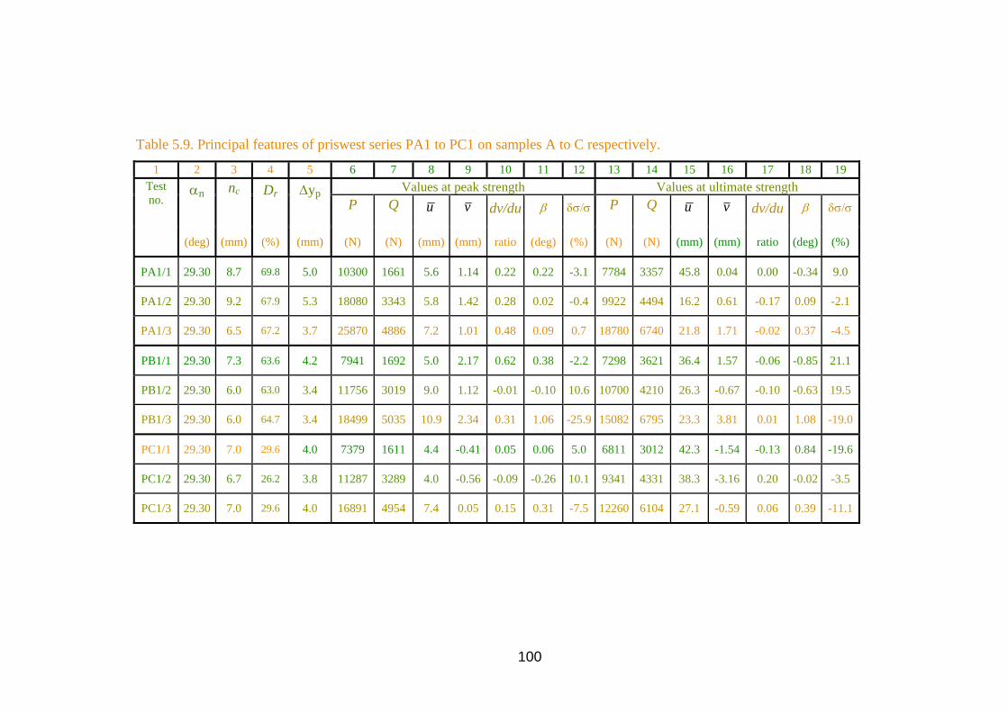
Table 5.9. Principal features of priswest series PA1 to PC1 on samples A to C respectively.
1 2 3 4 5 6 7 8 9 10 11 12 13 14 15 16 17 18 19 Values at peak strength Values at ultimate strength αn
nc
Dr
∆yp P Q u v dv/du β δσ/σ P Q u v dv/du β δσ/σ
Test no.
(deg) (mm) (%) (mm) (N) (N) (mm) (mm) ratio (deg) (%) (N) (N) (mm) (mm) ratio (deg) (%)
PA1/1 29.30 8.7 69.8 5.0 10300 1661 5.6 1.14 0.22 0.22 -3.1 7784 3357 45.8 0.04 0.00 -0.34 9.0
PA1/2 29.30 9.2 67.9 5.3 18080 3343 5.8 1.42 0.28 0.02 -0.4 9922 4494 16.2 0.61 -0.17 0.09 -2.1
PA1/3 29.30 6.5 67.2 3.7 25870 4886 7.2 1.01 0.48 0.09 0.7 18780 6740 21.8 1.71 -0.02 0.37 -4.5
PB1/1 29.30 7.3 63.6 4.2 7941 1692 5.0 2.17 0.62 0.38 -2.2 7298 3621 36.4 1.57 -0.06 -0.85 21.1
PB1/2 29.30 6.0 63.0 3.4 11756 3019 9.0 1.12 -0.01 -0.10 10.6 10700 4210 26.3 -0.67 -0.10 -0.63 19.5
PB1/3 29.30 6.0 64.7 3.4 18499 5035 10.9 2.34 0.31 1.06 -25.9 15082 6795 23.3 3.81 0.01 1.08 -19.0
PC1/1 29.30 7.0 29.6 4.0 7379 1611 4.4 -0.41 0.05 0.06 5.0 6811 3012 42.3 -1.54 -0.13 0.84 -19.6
PC1/2 29.30 6.7 26.2 3.8 11287 3289 4.0 -0.56 -0.09 -0.26 10.1 9341 4331 38.3 -3.16 0.20 -0.02 -3.5
PC1/3 29.30 7.0 29.6 4.0 16891 4954 7.4 0.05 0.15 0.31 -7.5 12260 6104 27.1 -0.59 0.06 0.39 -11.1
100

Table 5.10. Principal features of priswest series PA2 to PC2 on samples A to C respectively.
1 4 2 3 5 6 7 8 9 10 11 12 13 14 15 16 17 18 19 Values at peak strength αn
nc
Dr
∆yp P Q u v dv/du β δσ/σ P Q u v dv/du β δσ/σ
Test no.
(deg) (mm) (%) (mm) (N) (N) (mm) (mm) ratio (deg) (%) (N) (N) (mm) (mm) ratio (deg) (%)
PA2/1 39.91 6.8 69.8 3.5 25287 1625 4.5 -1.52 0.11 0.19 -4.6 19364 2937 13.5 -1.38 -0.10 0.28 -0.40
PA2/2 39.91 6.8 69.4 3.5 43982 3262 7.0 -2.81 0.16 0.54 -17.8 25105 6537 31.3 -1.06 -0.08 0.74 -6.60
PA2/3 39.91 6.8 68.3 3.5 50588 4900 9.8 0.90 0.21 1.04 -28.2 25980 6808 38.1 1.33 0.01 0.66 2.00
PB2/1 39.91 5.0 68.1 2.4 19744 1672 4.3 -0.59 0.14 0.29 -2.7 16736 4862 45.3 -1.65 -0.03 0.51 7.80
PB2/2 39.91 4.7 62.5 2.2 24932 3262 4.4 -1.71 0.23 0.34 -6.1 21407 6294 50.4 -1.77 -0.04 0.77 2.60
PB2/3 39.91 4.5 63.3 2.0 31519 4947 4.7 -1.92 0.30 0.25 -4.0 23840 6828 26.5 0.26 0.00 0.74 -3.70
PC2/1 39.91 4.9 24.3 2.3 12747 1665 2.6 -0.40 0.08 0.06 5.3 12066 3316 27.2 -0.51 -0.03 0.12 13.6
PC2/2 39.91 4.7 27.2 2.2 21213 3262 3.4 -2.28 -0.02 -0.01 3.2 19266 5448 41.3 -3.11 -0.05 1.05 -10.0
PC2/3 39.91 4.7 28.2 2.2 34234 4913 3.5 -1.87 0.14 0.29 -6.4 21016 5847 34.6 -1.95 -0.02 0.71 -2.1
Values at ultimate strength
101
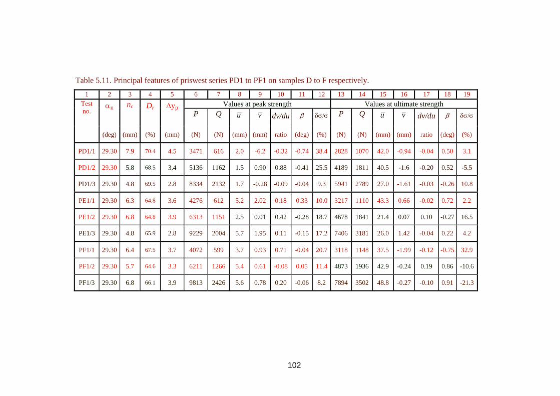
Table 5.11. Principal features of priswest series PD1 to PF1 on samples D to F respectively.
1 2 3 4 5 6 7 8 9 10 11 12 13 14 15 16 17 18 19 Values at peak strength Values at ultimate strength αn
nc
Dr
∆yp P Q u v dv/du β δσ/σ P Q u v dv/du β δσ/σ
Test no.
(deg) (mm) (%) (mm) (N) (N) (mm) (mm) ratio (deg) (%) (N) (N) (mm) (mm) ratio (deg) (%)
PD1/1 29.30 7.9 70.4 4.5 3471 616 2.0 -6.2 -0.32 -0.74 38.4 2828 1070 42.0 -0.94 -0.04 0.50 3.1
PD1/2 29.30 5.8 68.5 3.4 5136 1162 1.5 0.90 0.88 -0.41 25.5 4189 1811 40.5 -1.6 -0.20 0.52 -5.5
PD1/3 29.30 4.8 69.5 2.8 8334 2132 1.7 -0.28 -0.09 -0.04 9.3 5941 2789 27.0 -1.61 -0.03 -0.26 10.8
PE1/1 29.30 6.3 64.8 3.6 4276 612 5.2 2.02 0.18 0.33 10.0 3217 1110 43.3 0.66 -0.02 0.72 2.2
PE1/2 29.30 6.8 64.8 3.9 6313 1151 2.5 0.01 0.42 -0.28 18.7 4678 1841 21.4 0.07 0.10 -0.27 16.5
PE1/3 29.30 4.8 65.9 2.8 9229 2004 5.7 1.95 0.11 -0.15 17.2 7406 3181 26.0 1.42 -0.04 0.22 4.2
PF1/1 29.30 6.4 67.5 3.7 4072 599 3.7 0.93 0.71 -0.04 20.7 3118 1148 37.5 -1.99 -0.12 -0.75 32.9
PF1/2 29.30 5.7 64.6 3.3 6211 1266 5.4 0.61 -0.08 0.05 11.4 4873 1936 42.9 -0.24 0.19 0.86 -10.6
PF1/3 29.30 6.8 66.1 3.9 9813 2426 5.6 0.78 0.20 -0.06 8.2 7894 3502 48.8 -0.27 -0.10 0.91 -21.3
102

Table 5.12. Principal features of priswest series PD2 to PF2 on samples D to F respectively.
1 2 3 4 5 6 7 8 9 10 11 12 13 14 15 16 17 18 19 Values at peak strength Values at ultimate strength αn
nc
Dr
∆yp P Q u v dv/du β δσ/σ P Q u v dv/du β δσ/σ
Test no.
(deg) (mm) (%) (mm) (N) (N) (mm) (mm) ratio (deg) (%) (N) (N) (mm) (mm) ratio (deg) (%)
PD2/1 39.91 4.9 69.0 2.3 11995 1679 3.6 0.22 0.20 0.17 3.8 11020 3046 28.5 0.19 -0.02 1.20 -11.7
PD2/2 39.91 4.8 71.4 2.2 20941 3337 3.8 0.71 0.15 -0.08 9.0 18236 5116 34.9 0.51 -0.12 1.15 -12.0
PD2/3 39.91 5.2 66.2 2.5 25235 4981 5.4 0.56 0.15 0.27 -1.9 20967 6226 24.2 1.49 0.16 1.05 -11.7
PE2/1 39.91 5.7 64.0 2.8 17915 1683 3.9 -0.17 0.19 0.08 3.1 13555 3369 46.5 -2.55 -0.60 0.71 4.1
PE2/2 39.91 5.0 63.3 2.4 25979 3316 4.8 0.19 0.05 0.14 1.9 18822 4832 51.2 -0.67 -0.03 1.80 -22.5
PE2/3 39.91 5.2 63.3 2.5 33511 4940 7.4 2.11 0.22 0.32 -1.0 21352 5401 44.3 2.53 0.00 0.74 8.2
PF2/1 39.91 4.9 65.3 2.3 15909 1665 3.9 0.20 0.22 -0.08 10.7 12455 2937 30.3 1.37 -0.01 0.76 2.4
PF2/2 39.91 5.2 65.7 2.5 27273 3350 6.0 -0.49 0.12 0.32 -4.2 19072 3939 52.6 -1.53 0.02 1.18 -2.2
PF2/3 39.91 4.7 66.4 2.2 34219 4974 4.3 -1.28 0.07 -0.06 5.4 26078 5590 48.2 -2.09 -0.03 -0.02 30.0
103
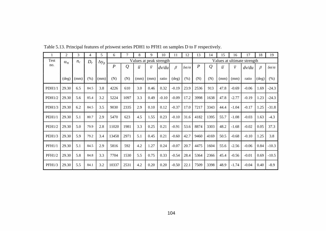
Table 5.13. Principal features of priswest series PDH1 to PFH1 on samples D to F respectively.
1 2 3 4 5 6 7 8 9 10 11 12 13 14 15 16 17 18 19Values at peak strength Values at ultimate strength αn
nc
Dr
∆yp P Q u v dv/du β δσ/σ P Q u v dv/du β δσ/σ
Test no.
(deg) (mm) (%) (mm) (N) (N) (mm) (mm) ratio (deg) (%) (N) (N) (mm) (mm) ratio (deg) (%)
PDH1/1 29.30 6.5 84.5 3.8 4226 610 3.0 0.46 0.32 -0.19 23.9 2536 913 47.8 -0.69 -0.06 1.69 -24.3
PDH1/2 29.30 5.6 85.4 3.2 5224 1097 3.3 0.49 -0.10 -0.09 17.2 3998 1638 47.8 -2.77 -0.19 1.23 -24.3
PDH1/3 29.30 6.2 84.5 3.5 9030 2335 2.9 0.10 0.12 -0.37 17.0 7217 3343 44.4 -1.04 -0.17 1.25 -31.8
PEH1/1 29.30 5.1 80.7 2.9 5470 623 4.5 1.55 0.23 -0.10 31.6 4182 1395 55.7 -1.08 -0.03 1.63 -4.3
PEH1/2 29.30 5.0 79.9 2.8 11020 1981 3.3 0.25 0.21 -0.91 53.6 8874 3303 48.2 -1.68 -0.02 0.05 37.3
PEH1/3 29.30 5.9 79.2 3.4 13458 2971 5.1 0.45 0.21 -0.60 42.7 9460 4169 50.5 -0.68 -0.10 1.25 3.8
PFH1/1 29.30 5.1 84.5 2.9 5816 592 4.2 1.27 0.24 -0.07 20.7 4475 1604 55.6 -2.56 -0.06 0.84 -10.3
PFH1/2 29.30 5.8 84.8 3.3 7704 1530 5.5 0.75 0.33 -0.54 28.4 5364 2366 45.4 -0.56 -0.01 0.69 -10.5
PFH1/3 29.30 5.5 84.1 3.2 10337 2531 4.2 0.20 0.20 -0.50 22.1 7509 3398 48.9 -1.74 -0.04 0.40 -8.9
104

Table 5.14. Principal features of priswest series PDH2 to PFH2 on samples D to F respectively.
1 2 3 4 5 6 7 8 9 10 11 12 13 14 15 16 17 18 19Values at peak strength Values at ultimate strength αn
nc
Dr
∆yp P Q u v dv/du β δσ/σ P Q u v dv/du β δσ/σ
Test no.
(deg) (mm) (%) (mm) (N) (N) (mm) (mm) ratio (deg) (%) (N) (N) (mm) (mm) ratio (deg) (%)
PDH2/1 39.91 5.8 84.0 2.9 21845 2261 4.0 1.29 0.32 0.18 0.9 15018 4748 60.6 1.52 -0.15 0.64 11.6
PDH2/2 39.91 5.4 85.4 2.6 28964 3330 2.1 -0.22 0.15 -0.02 3.4 22625 7167 56.2 -2.22 0.01 0.63 4.0
PDH2/3 39.91 5.9 85.0 2.9 35107 5013 3.9 -0.65 0.14 0.18 -3.5 22040 6984 56.8 -2.05 -0.01 1.02 -7.8
PEH2/1 39.91 5.6 79.5 2.7 24327 2274 4.9 -0.01 0.18 0.55 -12.0 19894 5279 53.9 -1.28 -0.08 0.77 4.4
PEH2/2 39.91 4.9 80.3 2.3 33352 3370 6.0 -0.01 0.07 0.49 -8.9 27403 7363 58.1 -1.88 -0.03 1.07 -3.7
PEH2/3 39.91 4.9 80.7 2.3 38618 5035 6.7 -0.06 0.12 0.63 -13.2 27988 7471 57.3 -1.84 -0.08 1.37 -13.5
PFH2/1 39.91 5.2 84.8 2.5 22332 2288 6.1 0.13 0.14 0.39 -4.6 16969 4568 49.8 -1.40 0.02 1.18 -9.2
PFH2/2 39.91 5.3 84.1 2.6 29009 3398 5.1 -0.43 0.07 0.23 -2.3 21747 6206 59.5 -2.55 -0.12 0.95 -1.7
PFH2/3 39.91 6.0 83.8 3.0 37680 5051 5.5 -0.58 0.09 0.26 -5.1 26233 7187 50.7 -2.03 0.00 0.64 4.6
105

0 10 20 30
-100
0
100
200
(kPa
)
(a)
τ
40 (mm) (mm)
0 10 20 30 (mm)
40-4
0
4
(m
m)
uu
(b)
0 10 20 30 (mm)
40-4
4
u u (mm)
(m
m)
β
β (d
eg)
0
0 10 20 30 (mm)
40-2
0
2
dv/d
u (m
m)
Figure 5.11. Typical curves for series PB1 of the variation with u of (a) τ, (b) v ,
(c) β, and (d) dv/du
σ PB1/1 � PB1/2 υ PB1/3
(c)
(d)
dv/d
u (r
atio
)
u
u
u (mm)
(mm) u
106

107
0 10 20 30 4 (mm
-50
0
50
100
150
200
(kPa
)
τ (a)
0)
u (
(mm)
0 10 20 30 (mm)
40-2
0
2
(deg
)
0 10 20 30-2
2
0
(m
m)
40
(mm)
u
(mm)
-10 10 20 30 40
(mm)
0
1
dv/d
u (ra
tio)
ure 5.12. Typical curves for s f the variation with Fig
σ PD2/1 � PD2/2 υ PD2/3
(c
(d)
β
u
u (mm)
mm)
u
u
dv/
du (r
atio
)
β (d
eg)
)
b) (
u of (a) τ, (b) veries PD2 o ,
(c) β, and (d) dv/du
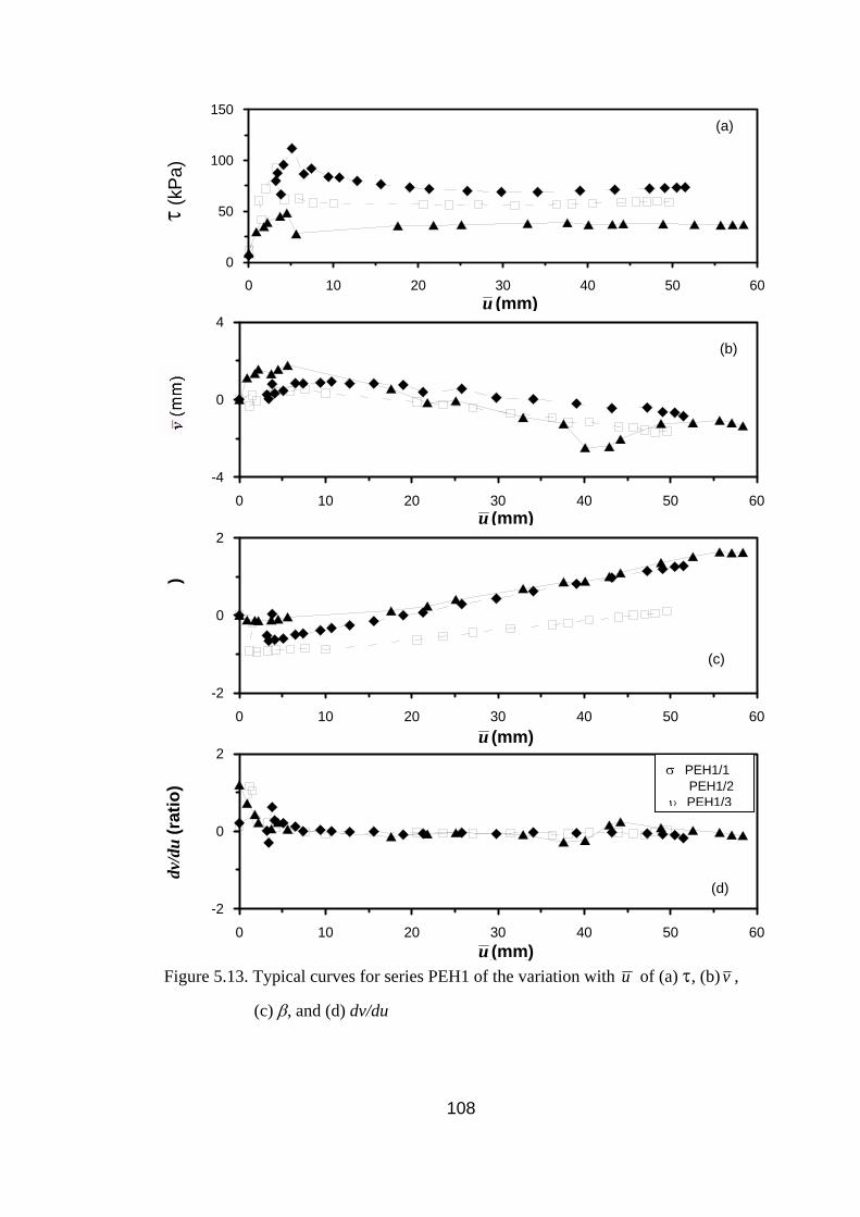
0 10 20 30 40 50 (mm)
600
50
100
150
(kPa
)
(a)
τ
0 10 20 30 40 50 (mm)
60-4
0
4
0 10 20 30 40 50
0 10 20 30 40 50 (mm)
60-2
0
2
dv/d
u (ra
tio)
u (mm)
(b)
(m
m)
_
60 (mm)
-2
2
0
(deg
)
β
β
(deg
Figure 5.13. Typical curves for series PEH1 of the variation with u of (a) τ, (b) v ,
(c) β, and (d) dv/du
σ PEH1/1 � PEH1/2 υ PEH1/3
(d)
(c)
u
u (mm)
u (mm)
u (mm)
dv/
du (r
atio
) )
108

0 10 20 30 40 50 (mm)
60-100
0
100
200
300
400
(kPa
)
0 10 20 30 40 50 (mm)
60-3
0
3
(m
m)
109
0 10 20 30 40 50 60 (mm)
0
β
1
2
(deg
)
0 10 20 30 40 50 (mm)
60-2
0
2
dv/d
u (ra
tio)
Figure 5.14. Typical curves for series PFH2 of the variation with u of (a) τ, (b) v ,
(c) β, and (d) dv/du
σ PFH2/1 � PFH2/2 υ PFH2/3
(d)
(c)
(b)
(a)
τ
u (mm)
u
u
(mm)
u (mm
u
)
u (mm)
d
v/du
(rat
io)
β (d
eg)
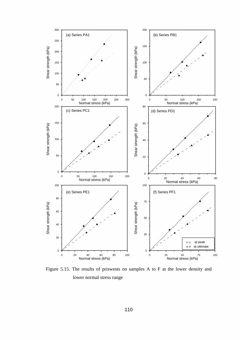
0 50 100 150 200 250 300Normal stress (kPa)
0
50
100
150
200
250
300
Shea
r stre
ngth
(kPa
)
0 50 100 150 200Normal stress (kPa)
0
50
100
150
200
Shea
r stre
ngth
(kPa
)
0 50 100 150 200Normal stress (kPa)
0
50
100
150
200
Shea
r stre
ngth
(kPa
)
0 20 40 60 8Normal stress (kPa)
00
20
40
60
80
Shea
r stre
ngth
(kPa
)
0 20 40 60 80 1Normal stress (kPa)
00 0 25 50 75Normal stress (kPa)
1000
25
50
75
100
Shea
r stre
ngth
(kPa
)
(a) Series PA1 (b) Series PB1
0
20
40
60
80
100
Shea
r stre
ngth
(kPa
)
Figure 5.15. The results of priswests on samples A to F at the lower density and
lower normal stress range
(c) Series PC1 (d) Series PD1
(e) Series PE1 (f) Series PF1
υ υ at peak σ σ at ultimate
110

0 100 200 300 400 500 600Normal stress (kPa)
0
100
200
300
400
500
600
Shea
r stre
ngth
(kPa
)
0 50 100 150 200 250 300Normal stress (kPa)
0
50
100
150
200
250
300
Shea
r stre
ngth
(kPa
)
0 50 100 150 200 250 300 350Normal stress (kPa)
0
50
100
150
200
250
300
350
Shea
r stre
ngth
(kPa
)
0 50 100 150 200 250Normal stress (kPa)
0
50
100
150
200
250
Shea
r stre
ngth
(kPa
)
0 50 100 150 200 250 300Normal stress (kPa)
0
50
100
150
200
250
0 50 100 150 200 250 300 350Normal stress (kPa)
0
50
100
150
200
250
300
300 350
(e) Series PE2 (f) Series PF2
Shea
r stre
ngth
(kPa
)
Shea
r stre
ngth
(kPa
)
Figure 5.16. The results of priswests on samples A to F at the lower density and
higher normal stress range
υ υ at peak σ σ at ultimate
(d) Series PD2 (c) Series PC2
(b) Series PB2 (a) Series PA2
111
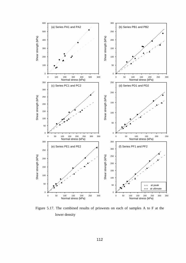
0 100 200 300 400 500 600Normal stress (kPa)
0
100
200
300
400
500
600
Shea
r stre
ngth
(kPa
)
0 50 100 150 200 250 300Normal stress (kPa)
0
50
100
150
200
250
300
Shea
r stre
ngth
(kPa
)
0 50 100 150 200 250 300 350Normal stress (kPa)
0
50
100
150
200
250
300
350
Shea
r stre
ngth
(kPa
)
0 50 100 150 200 250Normal stress (kPa)
0
50
100
150
200
250
Shea
r stre
ngth
(kPa
)
0 50 100 150 200 250 300Normal stress (kPa)
0
50
100
150
200
0 50 100 150 200 250 300 350Normal stress (kPa)
0
50
100
150
200
250
250
300
(kPa
)
(e) Series PE1 and PE2 (f) Series PF1 and PF2
300
Shea
r stre
ngth
(kPa
)
350
Shea
r stre
ngth
Figure 5.17. The combined results of priswests on each of samples A to F at the
lower density
d PA2 d PB2
d PC2 d PD2
υ υ at peak σ σ at ultimate
(d) Series PD1 an(c) Series PC1 an
(b) Series PB1 an(a) Series PA1 an
112

0 20 40 60 80 1Normal stress (kPa)
00 0 50 100 150 200 250 300 350Normal stress (kPa)
0
50
100
150
200
250
300
350
Shea
r stre
ngth
(kPa
)
0 20 40 60 80 100 12Normal stress (kPa)
0
0 20 40 60 80 1Normal stress (kPa)
00
0
20
40
60
80
100
Shea
r stre
ngth
(kPa
)
0
20
40
60
80
120
a)
100350(c) Series PEH1 (d) Series PEH2
0 50 100 150 200 250 300 350 400Normal stress (kPa)
0
50
100
150
200
250
300
400
Shea
r stre
ngth
(kPa
)
Shea
r stre
ngth
(kP
0
20
40
60
80
100
Shea
r stre
ngth
(kPa
)
0 50 100 150 200 250 300 350 400Normal stress (kPa)
0
50
100
150
200
250
300
350
400
Shea
r stre
ngth
(kPa
)
Figure 5.18. The results of priswests series on samples D to F at the higher density:
(a), (c), (e): lower normal stress range; (b), (d), (f): higher normal stress
range
(b) Series PDH2
(e) Series PFH1 (f) Series PFH2
υ υ at peak σ σ at ultimate
(a) Series PDH1
113

0 50 100 150 200 250 30
0 50 100 150 200 250 300 350 400Normal s
0 3No l s a
50rma stres (kP )
00
0
0
00
0 50 100N
150rma
200stres
250 (kP
300)
350 400o l s a
0
0
tress a (kP )
0
50
1
150
200
2
300
35
4
00
50
0
00
H1
σ at u teltima
5
100
150
200
250
300
350
400
Shea
r stre
ngth
(kPa
)
0
50
1
15
200
25
3
350
Shea
r stre
ngth
(kPa
)Sh
ear s
treng
th (k
Pa)
Figu
re 5.19. The combined results of priswests on each of samples D to F at the
higher density
(a) Series PDH1 and PDH2 (b) Series PE and PEH2
(c) Series PFH1 and PFH2
υ υ at peak σ
114
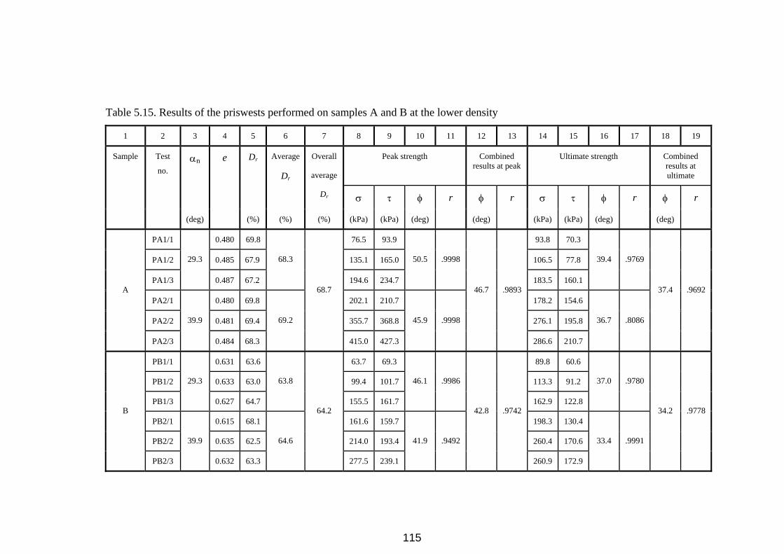
Table 5.15. Results of the priswests performed on samples A and B at the lower density
1 2 3 4 5 6 7 8 9 10 11 12 13 14 15 16 17 18 19
Peak strength Combined results at peak
Ultimate strength Combined results at ultimate
αn e Dr
Average
Dr
Overall
average
Dr σ τ φ r φ r σ τ φ r φ r
Sample
Test
no.
(deg) (%) (%) (%) (kPa) (kPa) (deg) (deg) (kPa) (kPa) (deg) (deg)
PA1/1 0.480 69.8 76.5 93.9 93.8 70.3
PA1/2 0.485 67.9 135.1 165.0 106.5 77.8
PA1/3
29.3
0.487
67.2
68.3
194.6 234.7
50.5 .9998
183.5 160.1
39.4 .9769
PA2/1 0.480 69.8 202.1 210.7 178.2 154.6
PA2/2 0.481 69.4 355.7 368.8 276.1 195.8
A
PA2/3
39.9
0.484
68.3
69.2
68.7
415.0 427.3
45.9 .9998
46.7 .9893
286.6 210.7
36.7 .8086
37.4 .9692
PB1/1 0.631 63.6 63.7 69.3 89.8 60.6
PB1/2 0.633 63.0 99.4 101.7 113.3 91.2
PB1/3
29.3
0.627
64.7
63.8
155.5 161.7
46.1 .9986
162.9 122.8
37.0 .9780
PB2/1 0.615 68.1 161.6 159.7 198.3 130.4
PB2/2 0.635 62.5 214.0 193.4 260.4 170.6
B
PB2/3
39.9
0.632
63.3
64.6
64.2
277.5 239.1
41.9 .9492
42.8 .9742
260.9 172.9
33.4 .9991
34.2 .9778
115

Table 5.16. Results of the priswests performed on samples C and D at the lower density
1 2 3 4 5 6 7 8 9 10 11 12 13 14 15 16 17 18 19
Peak strength Combined results at peak
Ultimate strength Combined results at ultimate
αn e Dr
Average
Dr
Overall
average
Dr σ τ φ r φ r σ τ φ r φ r
ample est
o.
(deg) (%) (%) (%) (kPa) (kPa) (deg) (deg) (kPa) (kPa) (deg) (deg)
PC1/1 0.556 29.6 60.7 63.2 83.1 58.2
99.1 93.3 78.4
C1/3
29.3 28.5 44.2 .9958 34.5 .9972
PC2/1 0.567 24.3 110.7 96.9 132.3 87.3
PC2/2 0.561 27.2 187.5 159.2 224.1 147.3
C2/3
39.9 26.6
27.5
295.6 262.6
41.2 .9986
41.9 .9937
236.5 158.9
33.6 .9990
33.8 .9984
PD1/1 0.647 70.4 29.5 29.1 35.1 23.2
PD1/2 0.651 68.5 43.7 42.5 51.3 33.9
D1/3
29.3 69.4
70.7 68.6
44.2 .9999
70.8 46.2
33.3 .9997
PD2/1 0.650 69.0 105.4 90.9 120.9 79.2
PD2/2 0.645 71.4 184.8 158.4 201.1 138.7
D2/3
39.9 68.9
69.2
231.0 186.7
39.7 .9936
40.1 .9949
226.0 149.2
33.8 .9958
33.8 .9991
S T
n
PC1/2 0.563 26.2 112.7
P 0.556 29.6 146.7 143.1
144.3 97.6
C
P 0.559 28.2
P 0.649 69.5
D
P 0.656 66.2
116

Table 5.17. Results of the priswests performed on samples E and F at the lower density
1 2 3 4 5 6 7 8 9 10 11 12 13 14 15 16 17 18 19
Peak strength Combined results at peak
Ultimate strength Combined results at ultimate
αn e Dr
Average
Dr
Overall
average
Dr σ τ φ r φ r σ τ φ r φ r
Sample
no.
Test
(deg) (%) (%) (%) (kPa) (kPa) (deg) (deg) (kPa) (kPa) (deg) (deg)
PE1/1 0.652 64.8 33.5 37.7 37.6 27.9
PE1/2 0.652 64.8 50.0 54.6 51.4 37.1
PE1/3
29.3
0.649
65.9
65.2
74.7 79.9
47.2 .9982
81.3 58.7
35.9 .9995
PE2/1 0.654 64.0 148.4 144.0 155.5 110.0
PE2/2 0.656 63.3 221.539.9 63.5
64.3 43.0 .9965 35.7 .9994
204.1 218.3 154.3
PE2/3 63.3 290.6 264.6 236.8 178.3
32.4 35.3 37.2 26.2
PF1/2 0.636 64.6 51.0 53.4 57.9 41.7
PE1/3 0.632
66.1
66.1
82.2 84.0
46.0 .9981
96.8 69.2
35.6 .9999
PF2/1 0.634 65.3 134.2 125.9 132.3 94.5
PF2/2 0.633 65.7 232.6 216.9 214.4 167.5
PF2/3
39.9
0.631 66.4
65.8
65.9
297.9 265.6
42.3 .9965
42.6 .9973
289.8 224.8
37.6 .9964
37.4 .9983
E
42.7 .9957 35.7 .9953
0.656
PF1/1 0.628 67.5
29.3
F
117

Table 5.18. Results of the priswests performed on samples D and E at the higher density
1 2 3 4 5 6 7 8 9 10 11 12 13 14 15 16 17 18 19
Peak strength Combined results at peak
Ultimate strength Combined results at ultimate
αn e Dr
Average
Dr
Overall
average
Dr σ τ φ r φ r σ τ φ r φ r
Sample
Test no.
(deg) (%) (%) (%) (kPa) (kPa) (deg) (deg) (kPa) (kPa) (deg) (deg)
PDH1/1 0.617 84.5 33.4 36.7 31.9 21.7
PDH1/2 0.615 85.4 43.7 43.9 50.1 34.2
PDH1/3
29.3
0.617
84.5
84.8
76.9 75.3
45.0 .9922
89.1 61.6
34.5 .9998
PDH2/1 0.618 84.0 180.9 175.9 191.7 124.5
PDH2/2 0.615 85.4 241.6 228.4 284.0 180.9
D
PDH2/3
39.9
0.616
85.0
84.8
84.8
302.2 273.2
42.9 .9857
43.0 .9981
276.3 177.9
32.7 .9989
32.8 .9995
PEH1/1 0.610 80.7 39.7 48.2 47.6 36.4
PEH1/2 0.612 79.9 82.7 93.1 97.6 74.5
PEH1/3
29.3
0.614 79.2
79.9
104.8 111.7
47.7 .9910
109.1 73.2
35.6 .9730
PEH2/1 0.613 79.5 199.5 198.0 235.5 166.5
PEH2/2 0.611 80.3 275.5 270.7 328.8 232.8
E
PEH2/3
39.9
0.610 80.7
80.2
80.0
328.9 306.9
43.8 .9871
44.2 .9950
332.9 237.8
35.4 .9995
35.4 .9993
118
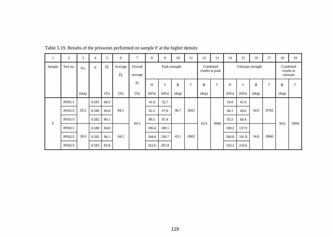
119
Table 5.19. Results of the priswests performed on sample F at the higher density
1 2 3 4 5 6 7 8 9 10 11 12 13 14 15 16 17 18 19
Peak strength Combined results at peak
Ultimate strength Combined results at ultimate
αBBn BB
e DBBr
Average
DBBrBB
OverallBB
average
DBBr BB σ τ φ r φ r σ τ φ r φ r
Sample Test no.
(deg) (%) (%) (%) (kPa) (kPa) (deg) (deg) (kPa) (kPa) (deg) (deg)
PFH1/1 0.581 84.5 41.9 52.7 54.0 41.0
PFH1/2 0.580 84.8 62.2 67.0 66.1 44.6
PFH1/3
29.3
0.582 84.1
84.5
86.5 87.4
46.7 .9261
93.5 64.4
34.9 .9782
PFH2/1 0.580 84.8 186.4 180.1 198.2 137.9
PFH2/2 0.582 84.1 244.6 230.7 268.8 181.8
F
PFH2/3
39.9
0.583 83.8
84.2
84.3
322.6 297.8
43.1 .9962
43.4 .9966
310.3 216.6
34.6 .9966
34.6 .9994
CHAPTER 6
TRIAXIAL TESTS PERFORMED
6.1 Introduction
To compare the results of wedge shear tests with those of triaxial tests,
triaxial tests were performed on samples A to F. In this chapter, the test procedure,
the order of testing the specimens, and the results of the tests are presented.
6.2 Test Procedure
This section has been mostly taken from Mirata (2000), and Gökalp (1994).
1. A 100 ml burette and the attached tubing were filled with deaired, distilled
water and connected to the pore pressure valve Vp of the cell (Fig. 6.1(b)); the pore
pressure ducts were flushed up to the top of the cell pedestal by opening the valve
Vp; then Vp was closed. The sides of the pedestal and the top cap were wiped dry and
smeared with castor oil for a better seal between the rubber membrane and these
components.
120

V3
V8
(b) Plan of base of
triaxial cell
(a) Some components of triaxial unit used
Figure 6.1. Triaxial apparatus used (adapted from Çağnan, 1990)
V4
Vp
GAUGE ON GAUGE OFF
V1 RIGHT UNIT IN USE LEFT UNIT IN USE
HPTCPU *
* HPTCPU : Hydraulic pump type constant pressure unit
BY - PASS
Triaxial cell
water
burette To
Copper tube
Vc
V2
V7
V5
V6
Pressure gauge
measurement device Volume change
121

2. Two 0.3 mm thick rubber membranes were passed through the three-part
split mould (Fig. 6.2); the ends turned over the mould and held by two rubber O-
rings at each end. The mould was placed on to the base plate, and the fastening
screws tightened moderately not to damage the membranes. The split ring SR (Fig.
6.3(b)), carrying three lugs L, displaced at 1200 with screw S welded on each, was
then clamped on to the mould as in Fig. 6.3(a). The collar C carrying three lugs with
holes engaging the screws S, was then placed on top of the mould, and the gap
between the collar and the top of the mould was adjusted by means of the nuts N so
as not to damage the rubber membranes (Fig. 6.4).
Figure 6.2. Rubber membranes on the three-part split mould with special attachment
(after Gökalp, 1994)
122
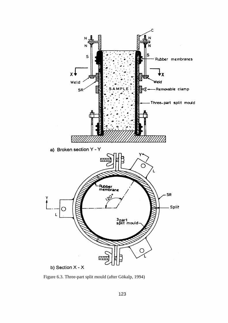
Figure 6.3. Three-part split mould (after Gökalp, 1994)
123

Figure 6.4. Three-part split mould with collar held gently above the rubber
membrane (after Gökalp, 1994)
3. For each sample prepared as in section 3.2, the amount of sand required to
give the same wet density as that obtained in cylwests and priswests was calculated.
This amount was compacted in the three-part split mould in five layers by the 2.5 kg
rammer to yield lower relative densities for samples A to F, and by the Kango
vibrating hammer to yield higher relative densities for samples D to F.
4. The collar and the split ring SR were removed and the top of the specimen
smoothed level with the top of the rubber membranes passing over the upper rim of
the mould. A perspex disc was held on top of the specimen and the whole inverted.
The base plate was replaced by a filter paper disc and a coarse porous stone, and the
whole re-inverted and placed on the cell pedestal. Another filter paper disc and a
coarse porous stone were placed on top of the specimen. The top cap was placed on
top; the ends of the rubber membranes were turned over the pedestal and the top cap.
124

The clamp of the mould was detached and the three segments of the mould removed.
During compaction using the Kango vibrating hammer, the membranes could be
damaged. So using a membrane placer, the outer membrane was replaced by an
intact membrane, and the damaged membrane was used during vibratory compaction
in subsequent tests. The rubber membranes were sealed with two rubber O-rings at
each end.
5. The cell ram was adjusted to just touch the top cap. To prevent buckling of
the loading system under high loads, the anti-friction guide (Fig. 6.5) was passed
over the cell ram for specimens at the higher density. The proving ring was mounted
in position, and the cell was raised until the ram just touched the proving ring
(Fig. 6.6).
6. The cell was filled with deaired distilled water using a separate tube
connected to the cell pressure valve Vc of the cell (Fig. 6.1(b)) to speed up the filling;
the air vent on top of the cell was closed. This tube was then disconnected and the
copper tube leading to the volume change measurement device (VCMD) (Fig. 6.1(a))
was connected to the valve Vc. The water level in the burette was adjusted to the
level of the mid-height of the specimen. This adjustment was done throughout the
test by lowering the burette when the specimen was compressed, and adding water to
the burette when the specimen dilated. If there was a hole in the membrane, after the
cell pressure was applied, the water level in the burette would rise continuously;
when this occurred, the test was stopped, and a new specimen prepared, using
undamaged membranes.
125

Figure 6.5. Top view of the anti-friction guide
Figure 6.6. Layout of triaxial cell with the anti-friction guide
126

7. The valve Vc on the cell was shut off. The valve V8 on the VCMD
(Fig. 6.1(a)) was set to the “bypass” position. By using the hydraulic pump type
constant pressure unit (HPTCPU), the cell pressure was built up to the desired value
to yield about the same average principal stress as that obtained in cylwests and
priswests. This cell pressure was calculated and output by the programs CYLWEE88
and IWPW77 (sections 5.1.5 and 5.2.5), assuming the angle between the shear plane
and the major principal stress in the wedge shear tests to be equal to (45o + φ/2)
(Appendix E). Valves V1, V3, and V4 were opened; valve V2 was set to “left unit in
use” position. Valves Vc and Vp on the cell were opened. During this procedure, due
to the compression of the specimen, and the penetration of the rubber membrane into
the soil pores, air was pressed out of the specimen pushing the water level in the
burette up. This level was restored to the level of the mid-height of the specimen by
removing some water from the burette if necessary.
8. The cell was left in this condition for about two hours. Then the valve V8
on the VCMD was shifted to the “read” position. When the volume change readings
became steady, the axial strain and proving ring dials were set to zero. The initial
burette readings on the VCMD were taken. The strain rate was set to 0.1 mm/min,
and axial loading was started. Axial strain, proving ring dial gauge, and the volume
change readings were taken at 10x10-3 inch intervals of axial compression. The test
was continued at this rate until the proving ring readings became steady or started to
drop. After the peak strength was reached, the strain rate was increased to
0.5 mm/min, but it was reduced to the original value of 0.1 mm/min and time was
allowed for the proving ring dial reading to become steady before taking the
readings. The test was continued until the proving ring readings become roughly
constant.
9. At the end of test, the compression machine was stopped; the valve V8 on
the VCMD was shifted to the “bypass” position. The cell pressure was reduced to
zero. The valve Vc on the cell and the valves V1, V3, and V4 were closed. The air
vent on top of the cell was opened. The axial load was removed by reversing the
127
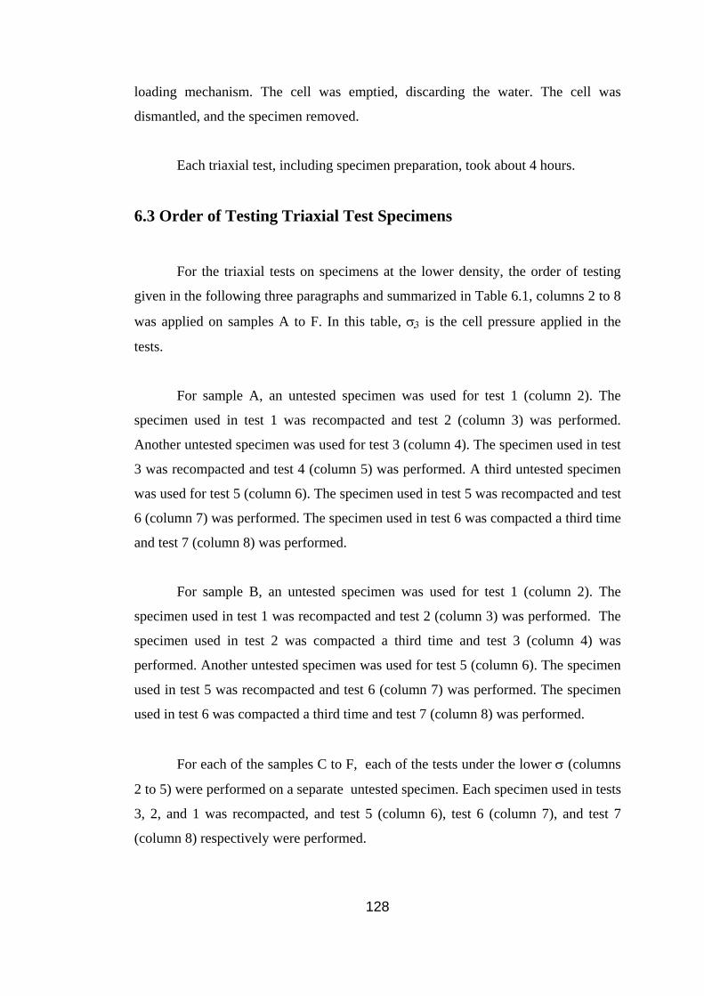
loading mechanism. The cell was emptied, discarding the water. The cell was
dismantled, and the specimen removed.
Each triaxial test, including specimen preparation, took about 4 hours.
6.3 Order of Testing Triaxial Test Specimens
For the triaxial tests on specimens at the lower density, the order of testing
given in the following three paragraphs and summarized in Table 6.1, columns 2 to 8
was applied on samples A to F. In this table, σ3 is the cell pressure applied in the
tests.
For sample A, an untested specimen was used for test 1 (column 2). The
specimen used in test 1 was recompacted and test 2 (column 3) was performed.
Another untested specimen was used for test 3 (column 4). The specimen used in test
3 was recompacted and test 4 (column 5) was performed. A third untested specimen
was used for test 5 (column 6). The specimen used in test 5 was recompacted and test
6 (column 7) was performed. The specimen used in test 6 was compacted a third time
and test 7 (column 8) was performed.
For sample B, an untested specimen was used for test 1 (column 2). The
specimen used in test 1 was recompacted and test 2 (column 3) was performed. The
specimen used in test 2 was compacted a third time and test 3 (column 4) was
performed. Another untested specimen was used for test 5 (column 6). The specimen
used in test 5 was recompacted and test 6 (column 7) was performed. The specimen
used in test 6 was compacted a third time and test 7 (column 8) was performed.
For each of the samples C to F, each of the tests under the lower σ (columns
2 to 5) were performed on a separate untested specimen. Each specimen used in tests
3, 2, and 1 was recompacted, and test 5 (column 6), test 6 (column 7), and test 7
(column 8) respectively were performed.
128
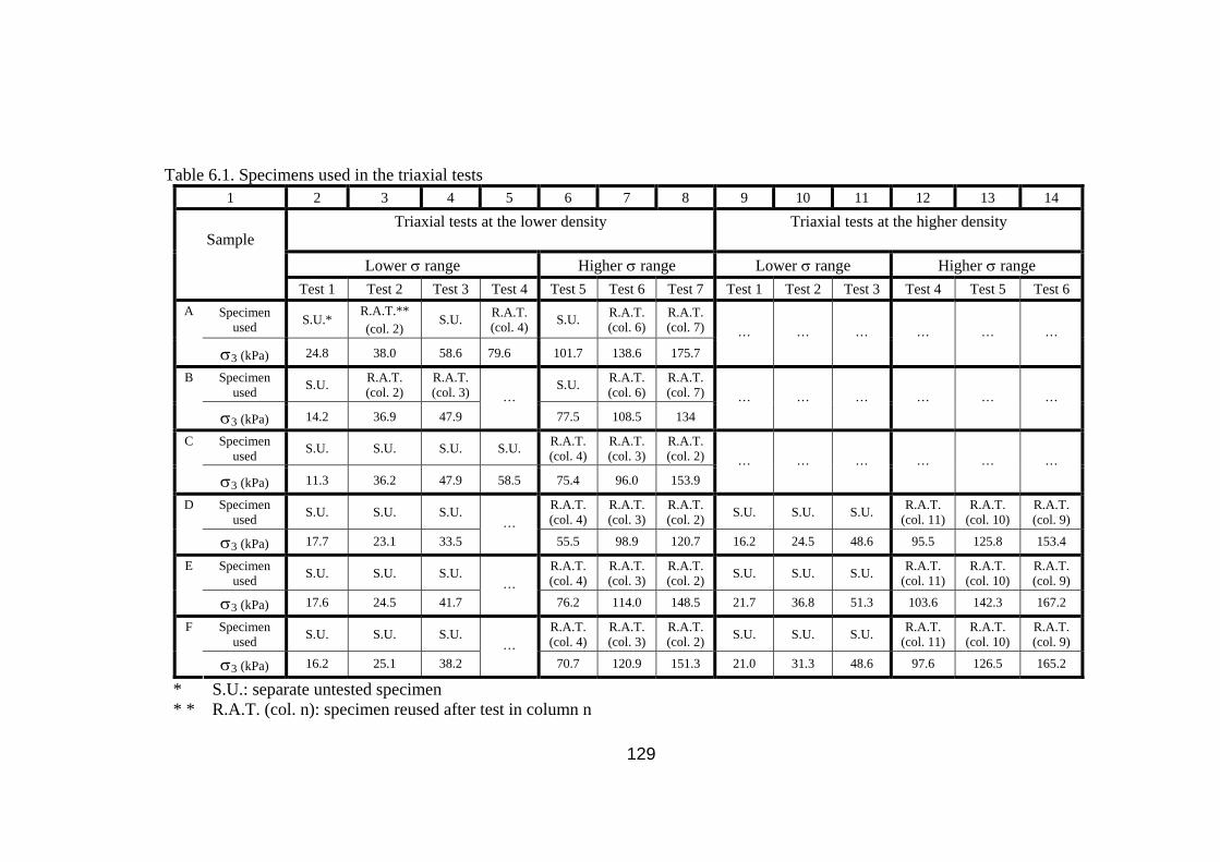
Table 6.1. Specimens used in the triaxial tests 1 2 3 4 5 6 7 8 9 10 11 12 13 14
Triaxial tests at the lower density Triaxial tests at the higher density
Lower σ range Higher σ range Lower σ range Higher σ range
Sample
Test 1 Test 2 Test 3 Test 4 Test 5 Test 6 Test 7 Test 1 Test 2 Test 3 Test 4 Test 5 Test 6 Specimen
used S.U.* R.A.T.** (col. 2)
S.U. R.A.T. (col. 4) S.U. R.A.T.
(col. 6) R.A.T. (col. 7)
A
σ3 (kPa) 24.8
38.0 58.6 79.6 101.7 138.6 175.7… … … … … …
Specimen used S.U. R.A.T.
(col. 2) R.A.T. (col. 3) S.U. R.A.T.
(col. 6) R.A.T. (col. 7)
B
σ3 (kPa) 14.2
36.9 47.9…
77.5 108.5 134… … … … … …
Specimen used S.U. S.U. S.U. S.U. R.A.T.
(col. 4) R.A.T. (col. 3)
R.A.T. (col. 2)
C
σ3 (kPa) 11.3
36.2 47.9 58.5 75.4 96.0 153.9… … … … … …
Specimen used S.U. S.U. S.U. R.A.T.
(col. 4) R.A.T. (col. 3)
R.A.T. (col. 2) S.U. S.U. S.U. R.A.T.
(col. 11) R.A.T.
(col. 10) R.A.T. (col. 9)
D
σ3 (kPa) 17.7 23.1 33.5…
55.5 98.9 120.7 16.2 24.5 48.6 95.5 125.8 153.4
Specimen used S.U. S.U. S.U. R.A.T.
(col. 4) R.A.T. (col. 3)
R.A.T. (col. 2) S.U. S.U. S.U. R.A.T.
(col. 11) R.A.T.
(col. 10) R.A.T. (col. 9)
E
σ3 (kPa) 17.6 24.5 41.7…
76.2 114.0 148.5 21.7 36.8 51.3 103.6 142.3 167.2
Specimen used S.U. S.U. S.U. R.A.T.
(col. 4) R.A.T. (col. 3)
R.A.T. (col. 2) S.U. S.U. S.U. R.A.T.
(col. 11) R.A.T.
(col. 10) R.A.T. (col. 9)
F
σ3 (kPa) 16.2 25.1 38.2…
70.7 120.9 151.3 21.0 31.3 48.6 97.6 126.5 165.2
* S.U.: separate untested specimen * * R.A.T. (col. n): specimen reused after test in column n 129
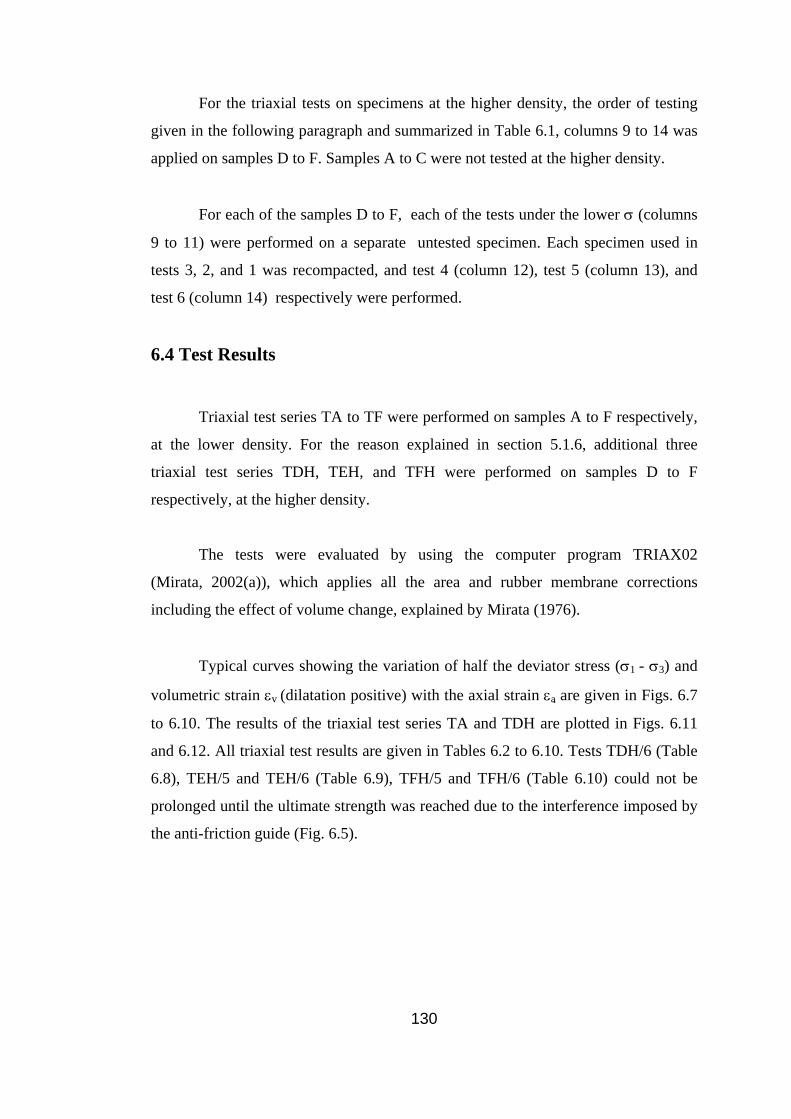
For the triaxial tests on specimens at the higher density, the order of testing
given in the following paragraph and summarized in Table 6.1, columns 9 to 14 was
applied on samples D to F. Samples A to C were not tested at the higher density.
For each of the samples D to F, each of the tests under the lower σ (columns
9 to 11) were performed on a separate untested specimen. Each specimen used in
tests 3, 2, and 1 was recompacted, and test 4 (column 12), test 5 (column 13), and
test 6 (column 14) respectively were performed.
6.4 Test Results
Triaxial test series TA to TF were performed on samples A to F respectively,
at the lower density. For the reason explained in section 5.1.6, additional three
triaxial test series TDH, TEH, and TFH were performed on samples D to F
respectively, at the higher density.
The tests were evaluated by using the computer program TRIAX02
(Mirata, 2002(a)), which applies all the area and rubber membrane corrections
including the effect of volume change, explained by Mirata (1976).
Typical curves showing the variation of half the deviator stress (σ1 - σ3) and
volumetric strain εv (dilatation positive) with the axial strain εa are given in Figs. 6.7
to 6.10. The results of the triaxial test series TA and TDH are plotted in Figs. 6.11
and 6.12. All triaxial test results are given in Tables 6.2 to 6.10. Tests TDH/6 (Table
6.8), TEH/5 and TEH/6 (Table 6.9), TFH/5 and TFH/6 (Table 6.10) could not be
prolonged until the ultimate strength was reached due to the interference imposed by
the anti-friction guide (Fig. 6.5).
130
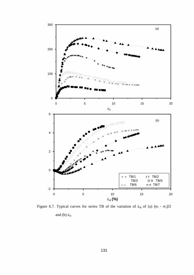
0 5 10 15 20
0
100
200
300
(kPa
)
(a)
(%) εa (%)
0 5 10 15 20 (%)
-2
0
2
4
6
(%)
(b)
εv
ε
v (%
)
(σ
- σ
)/21
3
(σ 1
- σ 3
)/2 (k
Pa)
ν ν TB/1 5 5 TB/2 � � TB/3 Η Η TB/5 υ υ TB/6 σ σ TB/7
εa (%)
Figure 6.7. Typical curves for series TB of the variation of εa of (a) (σ1 - σ3)/2
and (b) εv
131
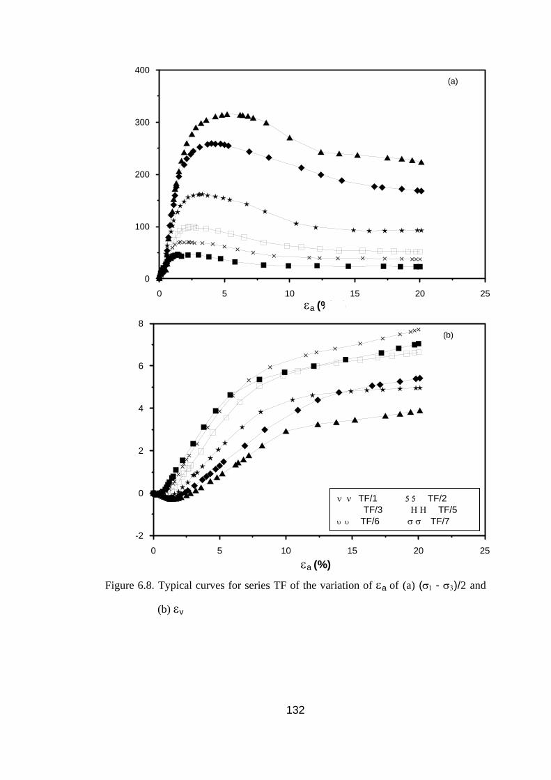
0 5 10 15 20 25
εa (%) (%)
0
100
200
300
400
(
kPa)
(a)
(σ 1
- σ 3
)/2
(
σ 1 -
σ 3)/2
(kPa
)
0 5 10 15 20 25 (%)
-2
0
2
4
6
8
(
%)
(b)
εv
ε v
(%)
ν ν TF/1 5 5 TF/2 � � TF/3 Η Η TF/5 υ υ TF/6 σ σ TF/7
εa (%)
Figure 6.8. Typical curves for series TF of the variation of εa of (a) (σ1 - σ3)/2 and
(b) εv
132
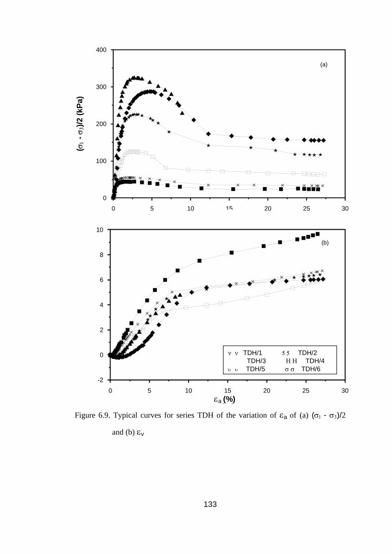
0 5 10 15 20 25 30
0
100
200
300
400
(k
Pa)
(a)
(
σ 1 -
σ 3)/2
(kPa
)
(%)εa (%)
0 5 10 15 20 25 30(%)
-2
0
2
4
6
8
10
(%)
(b)
εv
εv
(%)
ν ν TDH/1 5 5 TDH/2 � � TDH/3 Η Η TDH/4 υ υ TDH/5 σ σ TDH/6
εa εa (%)
Figure 6.9. Typical curves for series TDH of the variation of εa of (a) (σ1 - σ3)/2
and (b) εv
133
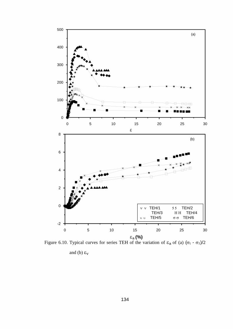
0 5 10 15 20 25 300
100
200
300
400
500
(k
Pa)
(a)
(σ1 -
σ3)/
2
(σ
1 - σ
3)/2
(kPa
)
(%) εa (%)
0 5 10 15 20 25 30(%)
-2
0
2
4
6
8
(%)
(b)
ε
v
ε v
(%)
ν ν TEH/1 5 5 TEH/2 � � TEH/3 Η Η TEH/4 υ υ TEH/5 σ σ TEH/6
Figure 6.10. Typical curves for series TEH of the variation of εa of (a) (σ1 - σ3)/2
and (b) εv
εa (%)
134
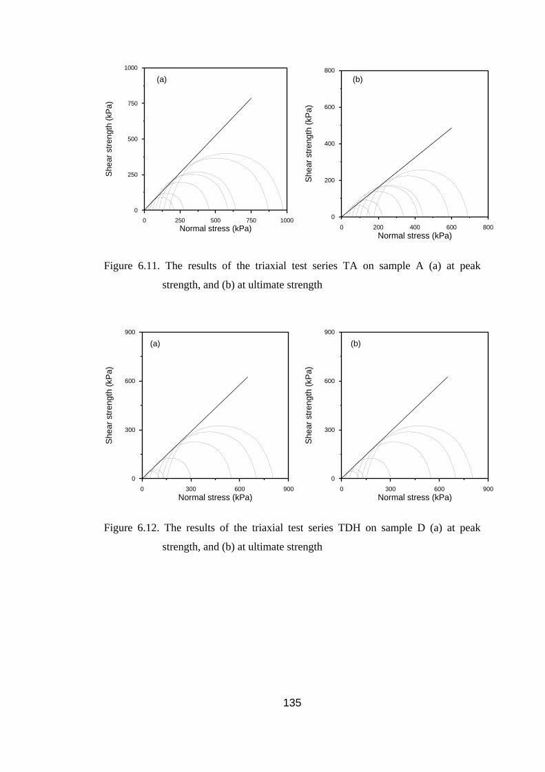
0 250 500 750 1000Normal stress (kPa)
0
250
500
750
1000
Shea
r stre
ngth
(kPa
)
0 200 400 600 800
Normal stress (kPa)
0
200
400
600
800
Shea
r stre
ngth
(kPa
)
(a) (b)
Figure 6.11. The results of the triaxial test series TA on sample A (a) at peak
strength, and (b) at ultimate strength
0 300 600 900Normal stress (kPa)
0
300
600
900
Shea
r stre
ngth
(kPa
)
0 300 600 900Normal stress (kPa)
0
300
600
900
Shea
r stre
ngth
(kPa
)
(a) (b)
Figure 6.12. The results of the triaxial test series TDH on sample D (a) at peak
strength, and (b) at ultimate strength
135
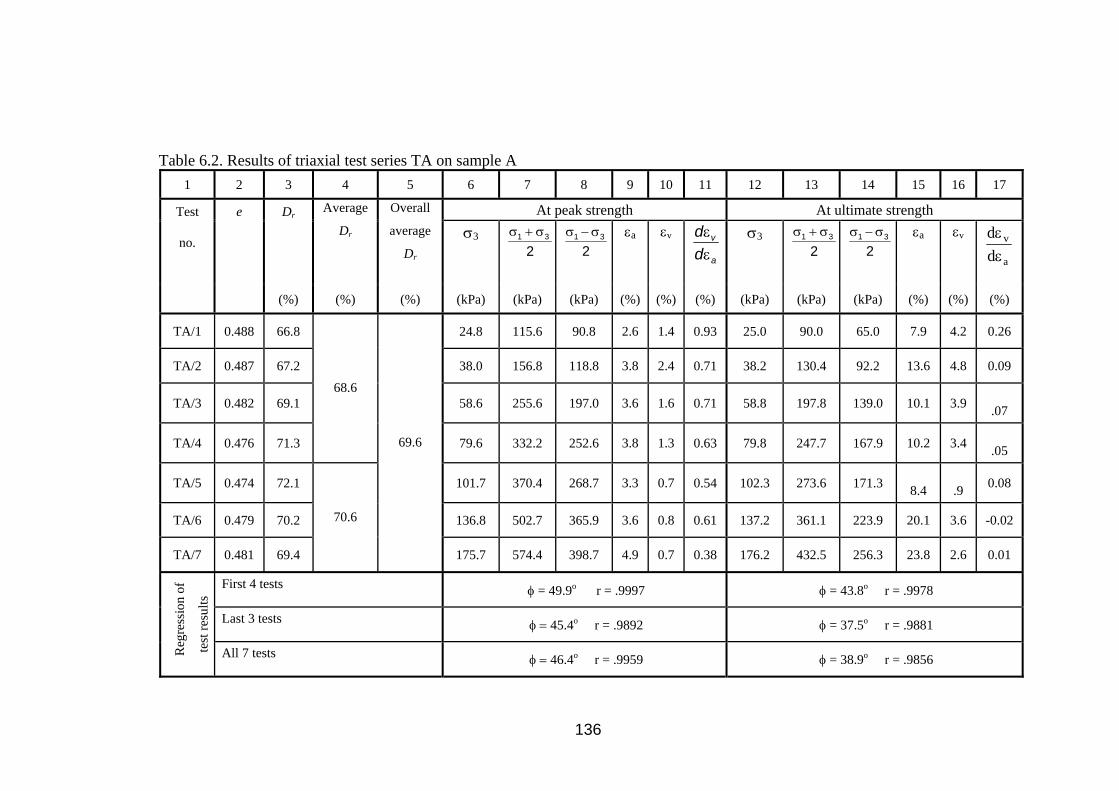
Table 6.2. Results of triaxial test series TA on sample A 1 2 3 4 5 6 7 8 9 10 11 12 13 14 15 16 17
At peak strength At ultimate strength DrAverage
Dr
Overall
average
Dr
σ32
31 σ+σ
2
31 σ−σ
εa
εv
σ32
31 σ+σ
2
31 σ−σ
εa
εv
a
v
dd
εε
Test
no.
e
(%) (%) (%) (kPa) (kPa) (kPa) (%) (%) (%) (kPa) (kPa) (kPa) (%) (%) (%)
TA/1 0.488 66.8 24.8 115.6 90.8 2.6 1.4 0.93 25.0 90.0 65.0 7.9 4.2 0.26
TA/2 0.487 67.2 38.0 156.8 118.8 3.8 2.4 0.71 38.2 130.4 92.2 13.6 4.8 0.09
TA/3 0.482 69.1 58.6 255.6 197.0 3.6 1.6 0.71 58.8 197.8 139.0 10.1 3.9 .07
TA/4 0.476 71.3
68.6
79.6 332.2 252.6 3.8 1.3 0.63 79.8 247.7 167.9 10.2 3.4 .05
TA/5 0.474 72.1 101.7 370.4 268.7 3.3 0.7 0.54 102.3 273.6 171.3 8.4 .9 0.08
TA/6 0.479 70.2 136.8 502.7 365.9 3.6 0.8 0.61 137.2 361.1 223.9 20.1 3.6 -0.02
TA/7 0.481 69.4
70.6
69.6
175.7 574.4 398.7 4.9 0.7 0.38 176.2 432.5 256.3 23.8 2.6 0.01
First 4 tests φ = 49.9o r = .9997 φ = 43.8o r = .9978
Last 3 tests φ = 45.4o r = .9892 φ = 37.5o r = .9881
R
egre
ssio
n of
test
resu
lts
All 7 tests φ = 46.4o r = .9959 φ = 38.9o r = .9856
a
v
dd
εε
136
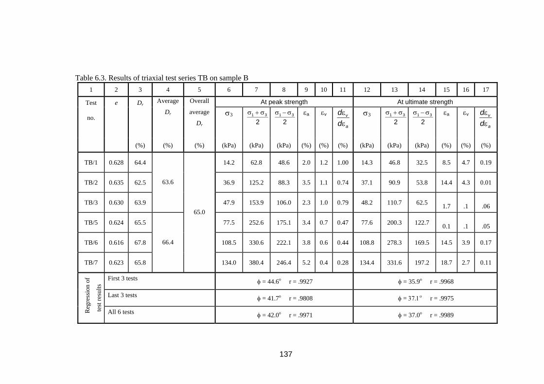
Table 6.3. Results of triaxial test series TB on sample B 1 2 3 4 5 6 7 8 9 10 11 12 13 14 15 16 17
At peak strength At ultimate strength DrAverage
Dr
Overall
average
Dr
σ32
31 σ+σ
2
31 σ−σ
εa
εv
σ32
31 σ+σ
2
31 σ−σ
εa
εv
a
v
dd
εε
Test
no.
e
(%) (%) (%) (kPa) (kPa) (kPa) (%) (%) (%) (kPa) (kPa) (kPa) (%) (%) (%)
TB/1 0.628 64.4 14.2 62.8 48.6 2.0 1.2 1.00 14.3 46.8 32.5 8.5 4.7 0.19
TB/2 0.635 62.5 36.9 125.2 88.3 3.5 1.1 0.74 37.1 90.9 53.8 14.4 4.3 0.01
TB/3 0.630 63.9
63.6
47.9 153.9 106.0 2.3 1.0 0.79 48.2 110.7 62.5 1.7 .1 .06
TB/5 0.624 65.5 77.5 252.6 175.1 3.4 0.7 0.47 77.6 200.3 122.7 0.1 .1 .05
TB/6 0.616 67.8 108.5 330.6 222.1 3.8 0.6 0.44 108.8 278.3 169.5 14.5 3.9 0.17
TB/7 0.623 65.8
66.4
65.0
134.0 380.4 246.4 5.2 0.4 0.28 134.4 331.6 197.2 18.7 2.7 0.11
First 3 tests φ = 44.6o r = .9927 φ = 35.9o r = .9968
Last 3 tests φ = 41.7o r = .9808 φ = 37.1ο r = .9975
R
egre
ssio
n of
test
resu
lts
All 6 tests φ = 42.0o r = .9971 φ = 37.0o r = .9989
a
v
dd
εε
137
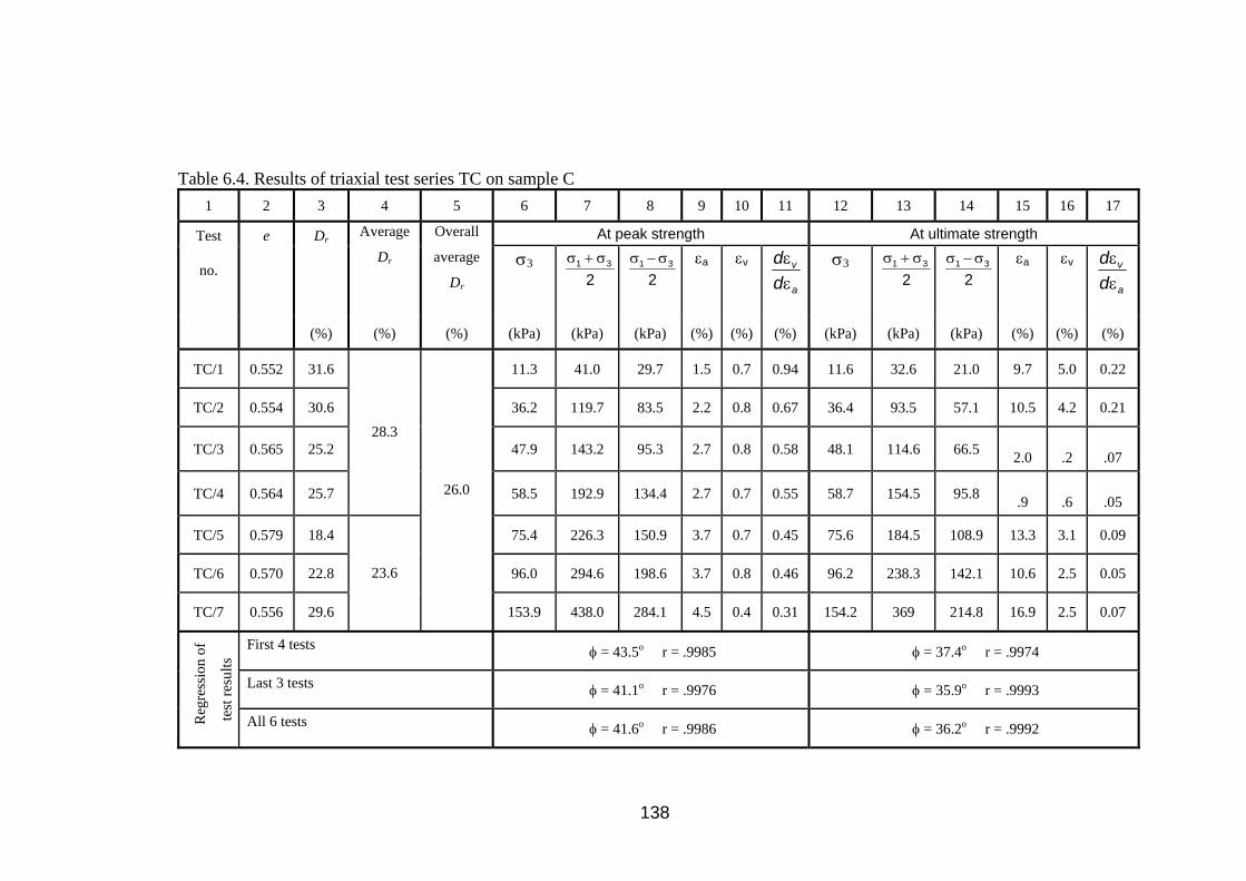
Table 6.4. Results of triaxial test series TC on sample C 1 2 3 4 5 6 7 8 9 10 11 12 13 14 15 16 17
At peak strength At ultimate strength DrAverage
Dr
Overall
average
Dr
σ32
31 σ+σ
2
31 σ−σ
εa
εv
σ32
31 σ+σ
2
31 σ−σ
εa
εv
a
v
dd
εε
Test
no.
e
(%) (%) (%) (kPa) (kPa) (kPa) (%) (%) (%) (kPa) (kPa) (kPa) (%) (%) (%)
TC/1 0.552 31.6 11.3 41.0 29.7 1.5 0.7 0.94 11.6 32.6 21.0 9.7 5.0 0.22
TC/2 0.554 30.6 36.2 119.7 83.5 2.2 0.8 0.67 36.4 93.5 57.1 10.5 4.2 0.21
TC/3 0.565 25.2 47.9 143.2 95.3 2.7 0.8 0.58 48.1 114.6 66.5 2.0 .2 .07
TC/4 0.564 25.7
28.3
58.5 192.9 134.4 2.7 0.7 0.55 58.7 154.5 95.8 .9 .6 .05
TC/5 0.579 18.4 75.4 226.3 150.9 3.7 0.7 0.45 75.6 184.5 108.9 13.3 3.1 0.09
TC/6 0.570 22.8 96.0 294.6 198.6 3.7 0.8 0.46 96.2 238.3 142.1 10.6 2.5 0.05
TC/7 0.556 29.6
23.6
26.0
153.9 438.0 284.1 4.5 0.4 0.31 154.2 369 214.8 16.9 2.5 0.07
First 4 tests φ = 43.5o r = .9985 φ = 37.4o r = .9974
Last 3 tests φ = 41.1o r = .9976 φ = 35.9o r = .9993
R
egre
ssio
n of
test
resu
lts
All 6 tests φ = 41.6o r = .9986 φ = 36.2o r = .9992
a
v
dd
εε
138
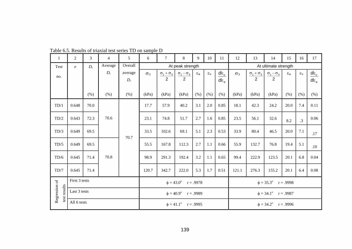
Table 6.5. Results of triaxial test series TD on sample D 1 2 3 4 5 6 7 8 9 10 11 12 13 14 15 16 17
At peak strength At ultimate strength DrAverage
Dr
Overall
average
Dr
σ32
31 σ+σ
2
31 σ−σ
εa
εv
σ32
31 σ+σ
2
31 σ−σ
εa
εv
a
v
dd
εε
Test
no.
e
(%) (%) (%) (kPa) (kPa) (kPa) (%) (%) (%) (kPa) (kPa) (kPa) (%) (%) (%)
TD/1 0.648 70.0 17.7 57.9 40.2 3.1 2.0 0.85 18.1 42.3 24.2 20.0 7.4 0.11
TD/2 0.643 72.3 23.1 74.8 51.7 2.7 1.6 0.85 23.5 56.1 32.6 8.2 .3 0.06
TD/3 0.649 69.5
70.6
33.5 102.6 69.1 5.1 2.3 0.53 33.9 80.4 46.5 20.0 7.1 .17
TD/5 0.649 69.5 55.5 167.8 112.3 2.7 1.1 0.66 55.9 132.7 76.8 19.4 5.1 .10
TD/6 0.645 71.4 98.9 291.3 192.4 3.2 1.1 0.65 99.4 222.9 123.5 20.1 6.8 0.04
TD/7 0.645 71.4
70.8
70.7
120.7 342.7 222.0 5.3 1.7 0.51 121.1 276.3 155.2 20.1 6.4 0.08
First 3 tests φ = 43.0o r = .9978 φ = 35.3o r = .9998
Last 3 tests φ = 40.9o r = .9989 φ = 34.1o r = .9987
R
egre
ssio
n of
test
resu
lts
All 6 tests φ = 41.1o r = .9995 φ = 34.2o r = .9996
a
v
dd
εε
139

Table 6.6. Results of triaxial test series TE on sample E 1 2 3 4 5 6 7 8 9 10 11 12 13 14 15 16 17
At peak strength At ultimate strength DrAverage
Dr
Overall
average
Dr
σ32
31 σ+σ
2
31 σ−σ
εa
εv
a
v
dd
εε
σ3
231 σ+σ
2
31 σ−σ
εa
εv
a
v
dd
εε
Test
no.
e
(%) (%) (%) (kPa) (kPa) (kPa) (%) (%) (%) (kPa) (kPa) (kPa) (%) (%) (%)
TE/1 0.654 64.0 17.6 70.3 52.7 1.9 0.8 1.00 18.1 45.8 27.7 20.0 5.6 0.12
TE/2 0.654 64.0 24.5 95.4 70.9 1.4 0.8 0.46 24.9 63.6 38.7 0.0 4.3 0.09
TE/3 0.651 65.2
64.4
41.7 156.9 115.2 2.4 0.9 0.97 42.1 102.4 60.3 0.1 .5 .08
TE/5 0.654 64.0 76.2 267.0 190.8 2.2 0.7 0.81 76.5 190.8 114.3 0.1 .4 .08
TE/6 0.651 65.2 114.0 362.5 248.5 3.7 0.7 0.48 114.4 288.1 173.7 20.1 3.5 0.14
TE/7 0.653 64.4
64.5
64.5
148.5 446.6 298.1 4.8 0.5 0.35 148.9 353.3 204.4 19.8 2.9 0.01
First 3 tests φ = 47.6o r = .9997 φ = 36.6o r = .9987
Last 3 tests φ = 43.0o r = .9895 φ = 36.1o r = .9961
R
egre
ssio
n of
te
st re
sults
All 6 tests φ = 43.4o r = .9976 φ = 36.2o r = .9994
140

Table 6.7. Results of triaxial test series TF on sample F 1 2 3 4 5 6 7 8 9 10 11 12 13 14 15 16 17
At peak strength At ultimate strength DrAverage
Dr
Overall
average
Dr
σ32
31 σ+σ
2
31 σ−σ
εa
εv
a
v
dd
εε
σ3
231 σ+σ
2
31 σ−σ
εa
εv
a
v
dd
εε
Test
no.
e
(%) (%) (%) (kPa) (kPa) (kPa) (%) (%) (%) (kPa) (kPa) (kPa) (%) (%) (%)
TF/1 0.636 64.6 16.2 63.0 46.8 1.4 0.7 1.08 16.7 39.7 23.0 20.0 7.1 0.16
TF/2 0.634 65.3 25.1 95.6 70.5 1.6 0.6 1.03 25.7 63.0 37.3 20.0 .7 0.14
TF/3 0.635 65.0
65.0
38.2 138.3 100.1 2.6 1.1 0.68 38.8 90.7 51.9 20.0 6.7 .10
TF/5 0.634 65.3 70.7 232.9 162.2 3.3 1.0 0.70 71.0 164.0 93.0 20.1 5.0 .02
TF/6 0.635 65.0 120.9 380.1 259.2 4.0 0.8 0.50 121.4 289.5 168.1 20.1 5.4 0.10
TF/7 0.632 66.1
65.4
65.2
151.3 466.6 315.3 5.2 0.9 0.42 151.7 375.5 223.8 20.1 3.9 0.10
First 3 tests φ = 46.9o r = .9993 φ = 35.4o r = .9988
Last 3 tests φ = 42.9ο r = .9992 φ = 36.0o r = .9985
R
egre
ssio
n of
te
st re
sults
All 6 tests φ = 43.2o r = .9992 φ = 36.0o r = .9996
141

Table 6.8. Results of triaxial test series TDH on sample D 1 2 3 4 5 6 7 8 9 10 11 12 13 14 15 16 17
At peak strength At ultimate strength DrAverage
Dr
Overall
average
Dr
σ32
31 σ+σ
2
31 σ−σ
εa
εv
σ32
31 σ+σ
2
31 σ−σ
εa
εv
a
v
dd
εε
Test
no.
e
(%) (%) (%) (kPa) (kPa) (kPa) (%) (%) (%) (kPa) (kPa) (kPa) (%) (%) (%)
TDH/1 0.615 85.4 16.2 60.5 44.3 1.4 1.0 1.12 17.0 40.5 23.5 26.5 9.7 0.19
TDH/2 0.618 84.0 24.5 79.7 55.2 2.5 1.6 0.84 25.1 57.8 32.7 6.5 6.6 0.12
TDH/3 0.616 85.0
84.8
48.6 174.2 125.6 2.4 0.9 0.90 49.3 112.9 63.6 6.5 .9 .18
TDH/4 0.617 84.5 95.5 321.6 226.1 2.7 1.0 0.83 96.1 212.6 116.5 26.0 6.4 .08
TDH/5 0.615 85.4 125.8 413.0 287.2 4.7 1.2 0.66 126.5 282.0 155.5 27.2 6.1 0.05
TDH/6 0.618 84.0
84.6
84.7
153.4 478.8 325.4 2.7 1.1 0.76 153.6 383.3 229.7 8.9 4.8 0.25
First 3 tests φ = 45.9o r = 0.9993 φ = 34.4o r = 0.9998
Last 3 tests φ = 43.6o r = 0.9952 φ = 35.2o r = 0.9876
R
egre
ssio
n of
te
st re
sults
All 6 tests φ = 43.8o r =0.9994 φ =35.2o r =0.9974
a
v
dd
εε
142

Table 6.9. Results of triaxial test series TEH on sample E 1 2 3 4 5 6 7 8 9 10 11 12 13 14 15 16 17
At peak strength At ultimate strength DrAverage
Dr
Overall
average
Dr
σ32
31 σ+σ
2
31 σ−σ
εa
εv
σ32
31 σ+σ
2
31 σ−σ
εa
εv
a
v
dd
εε
Test
no.
e
(%) (%) (%) (kPa) (kPa) (kPa) (%) (%) (%) (kPa) (kPa) (kPa) (%) (%) (%)
TEH/1 0.616 78.4 21.7 113.8 92.1 1.4 1.2 1.65 22.4 56.4 34.0 26.0 5.8 0.09
TEH/2 0.616 78.4 36.8 171.3 134.5 1.8 1.0 1.53 37.4 94.3 56.9 26.2 .7 0.01
TEH/3 0.611 80.3
79.0
51.3 214.5 163.2 2.0 0.8 1.30 51.9 128.5 76.6 26.9 4.2 .09
TEH/4 0.615 78.8 103.6 399.9 296.3 3.0 0.6 0.83 104.3 274.1 169.8 6.8 .9 .17
TEH/5 0.615 78.8 142.3 492.2 349.9 2.2 0.8 0.76 142.5 379.0 236.5 9.1 3.5 0.08
TEH/6 0.615 78.8
78.8
78.9
167.2 570.4 403.2 2.7 0.6 0.65 167.2 436.5 269.2 8.9 2.1 0.02
First 3 tests φ = 50.9o r = 0.9947 φ = 36.8o r = 0.9998
Last 3 tests φ = 45.7o r = 0.9884 φ = 38.3o r = 0.9996
R
egre
ssio
n of
test
resu
lts
All 6 tests φ = 46.2o r = 0.9972 φ = 38.2o r = 0.9998
a
v
dd
εε
143

Table 6.10. Results of triaxial test series TFH on sample F 1 2 3 4 5 6 7 8 9 10 11 12 13 14 15 16 17
At peak strength At ultimate strength DrAverage
Dr
Overall
average
Dr
σ32
31 σ+σ
2
31 σ−σ
εa
εv
σ32
31 σ+σ
2
31 σ−σ
εa
εv
a
v
dd
εε
Test
no.
e
(%) (%) (%) (kPa) (kPa) (kPa) (%) (%) (%) (kPa) (kPa) (kPa) (%) (%) (%)
TFH/1 0.579 85.2 21.0 96.5 75.5 1.1 0.3 1.40 21.8 51.6 29.8 26.5 9.0 0.22
TFH/2 0.580 84.8 31.3 137.3 106.0 2.0 1.0 1.26 32.0 73.6 41.6 6.9 5.9 0.10
TFH/3 0.580 84.8
84.9
48.6 207.2 158.6 2.2 0.9 1.17 49.2 116.7 67.5 5.3 .5 0.01
TFH/4 0.580 84.8 97.6 356.1 258.5 3.7 0.9 0.74 98.1 230.2 132.1 27.2 4.1 .05
TFH/5 0.582 84.1 126.5 428.7 302.2 3.0 0.8 0.66 126.6 336.1 209.5 9.1 3.0 0.06
TFH/6 0.579 85.2
84.7
84.8
165.2 517.6 352.4 3.9 1.1 0.47 165.2 487.2 322.0 8.5 3.0 0.36
First 3 tests φ = 50.3o r = 0.9997 φ = 35.1o r = 0.9995
Last 3 tests φ = 44.3o r = 0.9786 φ = 39.7o r = 0.9899
R
egre
ssio
n of
test
resu
lts
All 6 tests φ = 44.9o r = 0.9959 φ= 39.5o r = 0.9965
a
v
dd
εε
144
CHAPTER 7
SHEAR BOX TESTS PERFORMED
7.1 Introduction
To compare the results of wedge shear and triaxial shear tests with those of the
shear box tests, shear box tests were performed on previously untested specimens,
compacted directly in the shear box, at the lower density under the lower and higher
normal stress σ ranges. Shear box tests were also performed on specimens, taken
from the shear plane of previously sheared samples compacted in the cylwest and
priswest moulds, at the lower density under the lower σ range to study the effect on
shear strength of the orientation of the shear plane.
7.2 Description of Shear Box Test Apparatus
The following paragraphs have been mostly taken from Aybak (1988).
The shear box test apparatus (Fig. 7.1) has a shear box (a) split horizontally at
the level of the centre of the soil sample, which is held between metal grills and
porous stones. The upper and lower parts are held together by two retaining screws;
another two knurled screws are provided for raising the upper half relative to the
lower after the retaining screws are removed.
145
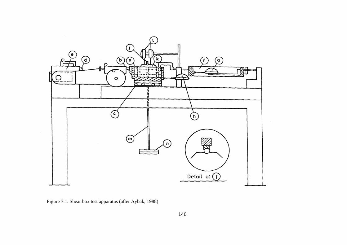
Figure 7.1. Shear box test apparatus (after Aybak, 1988)
146

A carrier (b), in which the box is placed, restrains the lower half of the box,
but allows free movement of the upper half. The carrier rests on a ball track (c) in
such a way that it can move only longitudinally. The movement of the carrier is
effected at a uniform rate by means of an electric motor (d) and a variable speed gear
box (e). The upper half of the box bears against a steel proving ring (f), whose
deformation is shown by a dial gauge (g), and can be converted into shearing force.
Another dial gauge (h) is attached to the bracket fixed to the main frame to measure
the shear displacement.
The vertical load is applied through a yoke (j) bearing on a metal pad (k),
which lies on top of the sample, and fits loosely into the shear box. Dead weights (n)
can be placed on a hanger (m) suspended from the yoke. A steel ball distributes the
load evenly over the sample while transmitting the load from the yoke to the pad.
Two dial gauges (l), which bear on the loading pad, are used for measuring vertical
displacement during shear, enabling also the slight rotation of the loading pad to be
calculated.
7.3 Shear Box Tests Performed on Specimens Compacted directly in
the Shear Box
7.3.1 Test Procedure
This section has been mostly taken from Mirata (2001). 60 mm x 60 mm
square specimens were used in all shear box tests. The components of the shear box
were similar to those shown in Fig. 7.2 for a circular shear box.
1. The shear box (Fig. 7.2) was cleaned, the inner walls were smeared with a
thin layer of silicone grease, and the two halves were screwed together. Ensuring that
the recesses on the retaining plate engaged the pins at the inner sides of the shear
box, this plate and the porous stone were placed in the bottom of the shear box,
followed by the serrated, perforated grid plate, making sure that the serrations faced
upwards and were at right angles to the direction of shear.
147
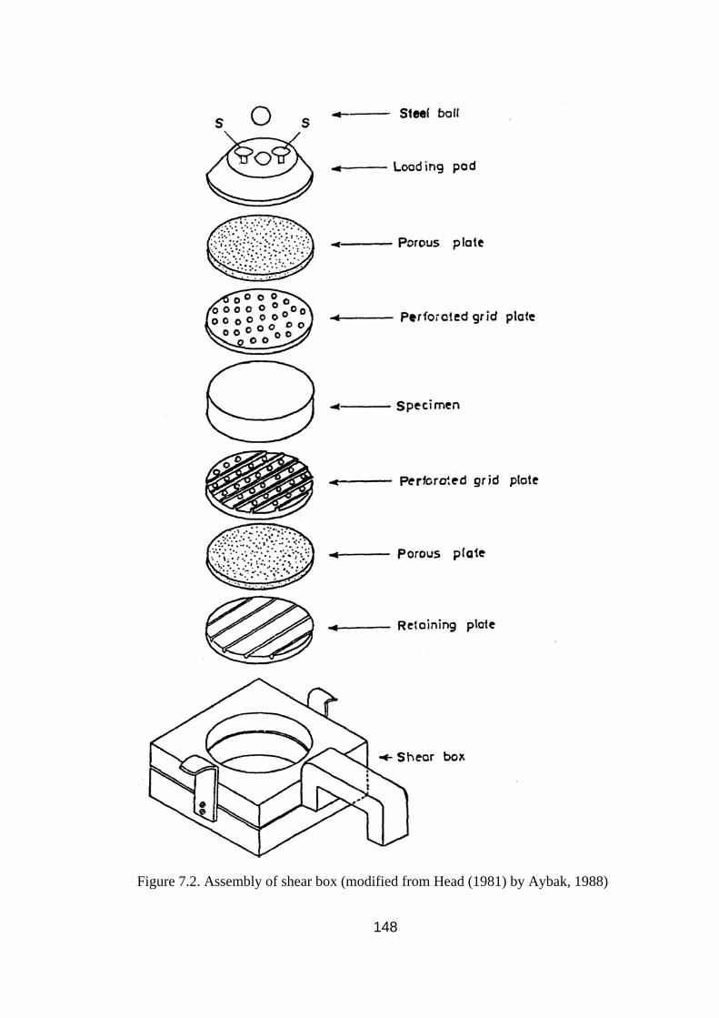
Figure 7.2. Assembly of shear box (modified from Head (1981) by Aybak, 1988)
148
2. For each sample prepared as in section 3.2, the amount of sand at the
desired water content to be placed in the shear box to from a 20 mm thick specimen
was calculated to yield the same wet density as that obtained in previous wedge shear
and triaxial shear tests. In calculating the volume of the specimen to be placed in the
shear box, the total volume of the serrations on the serrated grid plate was deducted,
and the total volume of the perforations on this plate was added. So, 0.35 cm3 was
deducted from the calculated volume of the specimen.
3. The height h1 (mm) from the flat part of the serrated plate to the top of the
shear box was measured. The sand, calculated at step 2, was placed in the shear box
in three layers. Each layer was tamped at such an intensity that when the whole
specimen had been placed in the shear box, the height between the top of the loading
pad, temporarily placed on top of the specimen, would be (h1 – 20 – tp) mm below
the top of the shear box, where tp (mm) was the thickness of the loading pad.
4. The upper serrated grid plate was placed on the specimen, with the
serrations facing downwards and at right angles to the direction of shear. The upper
porous stone was laid on top of the grid plate, and the loading pad was placed on top,
with the two studs S (Fig. 7.2) aligned in the direction of shear.
5. The shear box was placed into the carrier (b in Fig. 7.1), and the hanger
was set in position on the loading pad, with a cleaned and lubricated steel ball in
between. The two vertical displacement dials (l in Fig. 7.1), were set to bear on the
two studs S of the loading pad (k in Fig. 7.1), and adjusted to enable recording
displacements of at least 5 mm both ways. The horizontal distance between the tips
of these dial gauges was measured.
6. The additional dead weight Wd (lbf) to be placed on the hanger (without the
load magnification arm) was calculated from the following equations to give the
same normal stress σ (kPa) as that obtained from previous wedge shear tests, and
placed on the hanger.
149

48.44
AWtσ
= ………......………………………..(7.1)
08.13WW td −= ................…………………………(7.2)
where Wt (lbf) is the total dead weight on the specimen and A (cm2) is the area of the
specimen
7. The two knurled lifting screws were tightened until they just beared on the
lower half of the shear box. The two retaining screws were removed and the lifting
screws were given sufficient number of turns to make the clearance between the two
halves of the box slightly more than the largest size of the particle in the specimen.
(One full turn of such screws raised the upper half by 0.9 mm). Then the lifting
screws were loosened by more number of turns than they had been tightened.
8. The displacement rate was set to about 0.08 mm/min by choosing the
appropriate pair of gear wheels, and the right position of the gear lever. The initial
readings of the shear displacement dial, the vertical displacement dials, and the
proving ring dial were recorded.
9. The motor feed was engaged by turning the knurled knob at the rear of the
hand wheel until the tongue engaged the slot. The motor was switched on and
readings were taken at appropriate intervals until the peak strength was reached.
Then the displacement rate was increased by 5 times between readings, reducing this
rate to the initial value before taking the readings. Readings were continued until the
ultimate strength was reached.
10. The motor was stopped. The motor feed was disengaged, and the box was
reversed manually until the initial shear displacement was obtained. The pair of the
vertical displacement dial gauges were raised and turned to one side without
disturbing their horizontal distance from the shear box. The dead weights were lifted
off and the shear box was removed.
150

Each shear box test, including specimen preparation, took about 1 hour.
7.3.2 Test Results
Six shear box test series SA to SF of six tests each were performed on
samples A to F respectivelyssss. The tests were evaluated by using the computer
program DIST02 (Mirata, 2002(b)). The values output for no area correction and no
dilatation correction were taken.
Typical curves of the variation with shear displacement u of shear stress τ,
normal displacement v (positive values indicating dilatation), and the slight rotation
β of the loading pad (positive values indicating clockwise rotation when viewed as in
Fig. 7.1) are given in Figs. 7.3 and 7.4. Test results are plotted in Fig. 7.5, and
summarized in Tables 7.1 and 7.2.
151
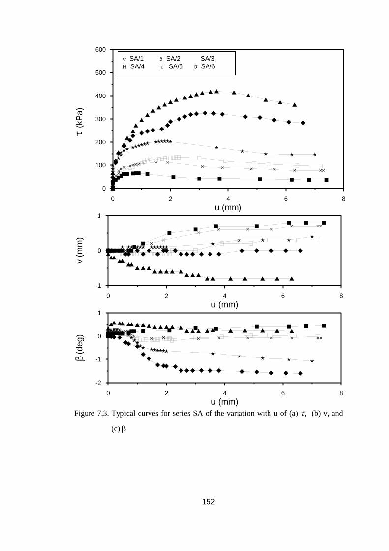
0 2 4 6u
8(mm)
0
100
200
300
400
500
600
(kPa
)
ν SA/1 5 SA/2 � SA/3 Η SA/4 υ SA/5 σ SA/6
τ
0 2 4 6 8u (mm)
-1
0
1
v (m
m)
0 2 4 6 8u (mm)
-2
-1
0
1
(
β
deg
)
Figure 7.3. Typical curves for series SA of the variation with u of (a) τ, (b) v, and
(c) β
152
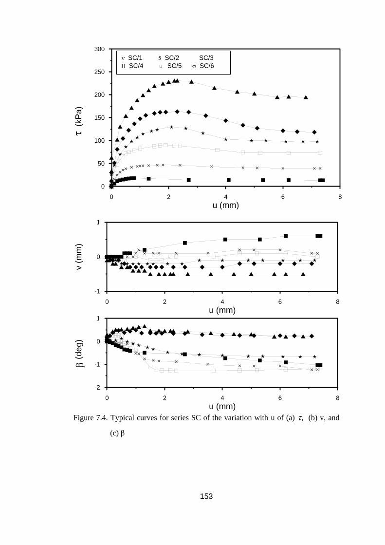
0 2 4 6u
8(mm)
0
50
100
150
200
250
300
(kPa
)
ν SC/1 5 SC/2 � SC/3 Η SC/4 υ SC/5 σ SC/6
0 2 4 6 8u (mm)
-1
0
1
v (m
m)
0 2 4 6 8u (mm)
-2
-1
0
1
(d
eg)
τ
β
Figure 7.4. Typical curves for series SC of the variation with u of (a) τ, (b) v, and
(c) β
153

0 100 200 300 400 500 600Normal stress (kPa)
0
100
200
300
400
500
600
Shea
r stre
ngth
(kPa
)
0 100 200 300 400Normal stress (kPa)
0
100
200
300
400
Shea
r stre
ngth
(kPa
)
0 100 200 300 400Normal stress (kPa)
0
100
200
300
400
Shea
r stre
ngth
(kPa
)
0 100 200 300Normal stress (kPa)
0
100
200
300
Shea
r stre
ngth
(kPa
)
0 100 200 300 400Normal stress (kPa)
0
100
200
300
400
Shea
r stre
ngth
(kPa
)
0 100 200 300 400Normal stress (kPa)
0
100
200
300
400
Shea
r stre
ngth
(kPa
)
(a) Series SA (b) Series SB
(c) Series SC (d) Series SD
(e) Series SE (f) Series SF
υ υ at peak σ σ at ultimate
Figure 7.5. The results of shear box tests performed on specimens compacted directly
in the shear box
154
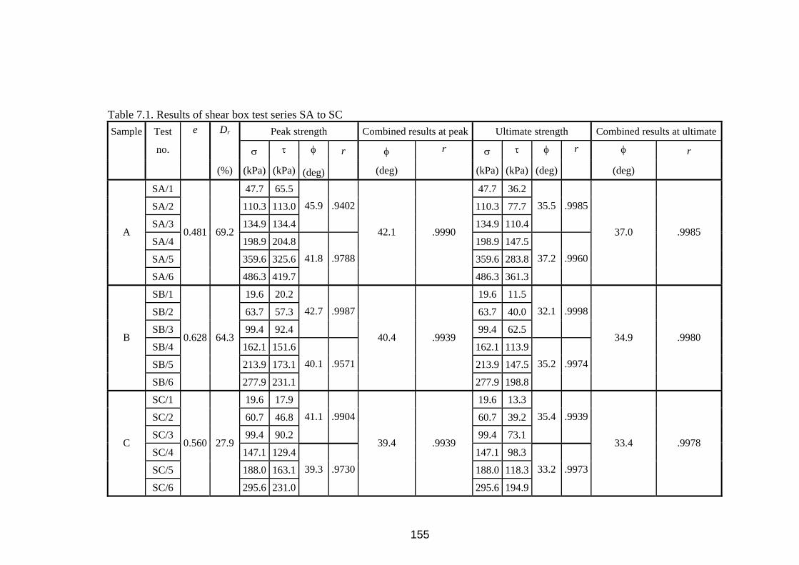
Table 7.1. Results of shear box test series SA to SC Peak strength Combined results at peak Ultimate strength Combined results at ultimate Dr
σ τ φ r φ r σ τ φ r φ r
Sample Test
no.
e
(%) (kPa) (kPa) (deg) (deg) (kPa) (kPa) (deg) (deg)
SA/1 47.7 65.5 47.7 36.2
SA/2 110.3 113.0 110.3 77.7
SA/3 134.9 134.4
45.9 .9402
134.9 110.4
35.5 .9985
SA/4 198.9 204.8 198.9 147.5
SA/5 359.6 325.6 359.6 283.8
A
SA/6
0.481 69.2
486.3 419.7
41.8 .9788
42.1 .9990
486.3 361.3
37.2 .9960
37.0 .9985
SB/1 19.6 20.2 19.6 11.5
SB/2 63.7 57.3 63.7 40.0
SB/3 99.4 92.4
42.7 .9987
99.4 62.5
32.1 .9998
SB/4 162.1 151.6 162.1 113.9
SB/5 213.9 173.1 213.9 147.5
B
SB/6
0.628 64.3
277.9 231.1
40.1 .9571
40.4 .9939
277.9 198.8
35.2 .9974
34.9 .9980
SC/1 19.6 17.9 19.6 13.3
SC/2 60.7 46.8 60.7 39.2
SC/3 99.4 90.2
41.1 .9904
99.4 73.1
35.4 .9939
SC/4 147.1 129.4 147.1 98.3
SC/5 188.0 163.1 188.0 118.3
C
SC/6
0.560 27.9
295.6 231.0
39.3 .9730
39.4 .9939
295.6 194.9
33.2 .9973
33.4 .9978
155
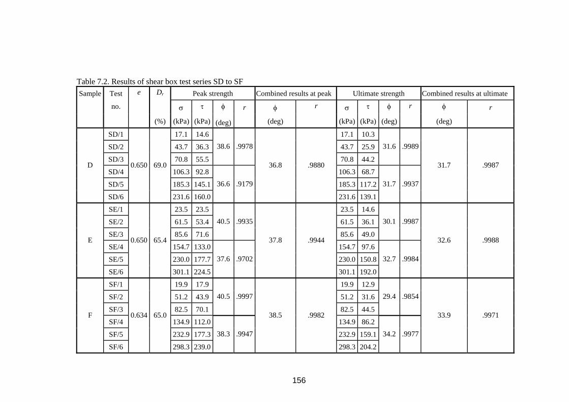
Table 7.2. Results of shear box test series SD to SF Peak strength Combined results at peak Ultimate strength Combined results at ultimate Dr
σ τ φ r φ r σ τ φ r φ r
Sample Test
no.
e
(%) (kPa) (kPa) (deg) (deg) (kPa) (kPa) (deg) (deg)
SD/1 17.1 14.6 17.1 10.3
SD/2 43.7 36.3 43.7 25.9
SD/3 70.8 55.5
38.6 .9978
70.8 44.2
31.6 .9989
SD/4 106.3 92.8 106.3 68.7
SD/5 185.3 145.1 185.3 117.2
D
SD/6
0.650 69.0
231.6 160.0
36.6 .9179
36.8 .9880
231.6 139.1
31.7 .9937
31.7 .9987
SE/1 23.5 23.5 23.5 14.6
SE/2 61.5 53.4 61.5 36.1
SE/3 85.6 71.6
40.5 .9935
85.6 49.0
30.1 .9987
SE/4 154.7 133.0 154.7 97.6
SE/5 230.0 177.7 230.0 150.8
E
SE/6
0.650 65.4
301.1 224.5
37.6 .9702
37.8 .9944
301.1 192.0
32.7 .9984
32.6 .9988
SF/1 19.9 17.9 19.9 12.9
SF/2 51.2 43.9 51.2 31.6
SF/3 82.5 70.1
40.5 .9997
82.5 44.5
29.4 .9854
SF/4 134.9 112.0 134.9 86.2
SF/5 232.9 177.3 232.9 159.1
F
SF/6
0.634 65.0
298.3 239.0
38.3 .9947
38.5 .9982
298.3 204.2
34.2 .9977
33.9 .9971
156

7.4 Shear Box Tests Performed on Specimens Taken from the Shear
Plane of Samples Compacted in the Cylwest and Priswest
Moulds 7.4.1 Introduction
The results obtained from the wedge shear tests on samples A to F (section
8.1.1, paragraph (4)) had shown that the values of peak friction angles obtained from
cylwests under the lower normal stresses were higher than those obtained from
priswests using the 30o mould. In order to investigate the reason of this difference,
samples used in previous shear tests were compacted in the cylwest and priswest
moulds, and shear box tests were performed on specimens taken from the shear plane
of these samples under the lower σ ranges.
7.4.2 Preparation of the Samples
Sample A was inadvertently discarded after the previous shear tests had been
completed. Samples B to F, already used in previous shear tests, were in a slightly
moist condition. So each of the samples were first air-dried by spreading them in a
large tray as a layer of about 5 cm thickness and thoroughly mixing them several
times during the day. Each sample was then mixed thoroughly and separated into
representative sub-samples by passing through the riffle box. In this way were
prepared one 40-kg sub-sample for compaction in the priswest mould, two 8-kg
sub-samples for compaction in the cylwest mould, and one 2-kg sub-sample for the
granulometric analyses. The grain size curves of the original samples and the
samples taken for shear box tests are shown in Figs. 7.6 to 7.10.
157
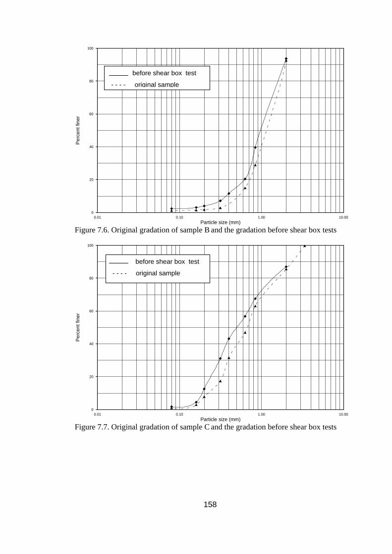
0.01 0.10 1.00 10.00Particle size (mm)
0
20
40
60
80
100
Perc
ent f
iner
Figure 7.6. Original gradation of sample B and the gradation before shear box tests
0.01 0.10 1.00 10.00Particle size (mm)
0
20
40
60
80
100
Perc
ent f
iner
before shear box test
- - - - original sample
before shear box test
- - - - original sample
Figure 7.7. Original gradation of sample C and the gradation before shear box tests
158
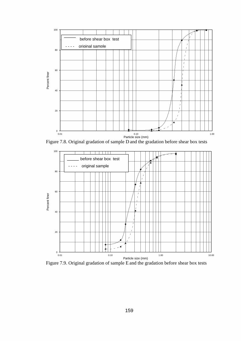
0.01 0.10 1.00Particle size (mm)
0
20
40
60
80
100
Perc
ent f
iner
Figure 7.8. Original gradation of sample D and the gradation before shear box tests
0.01 0.10 1.00 10.00Particle size (mm)
0
20
40
60
80
100
Perc
ent f
iner
before shear box test
- - - - original sample
before shear box test
- - - - original sample
Figure 7.9. Original gradation of sample E and the gradation before shear box tests
159
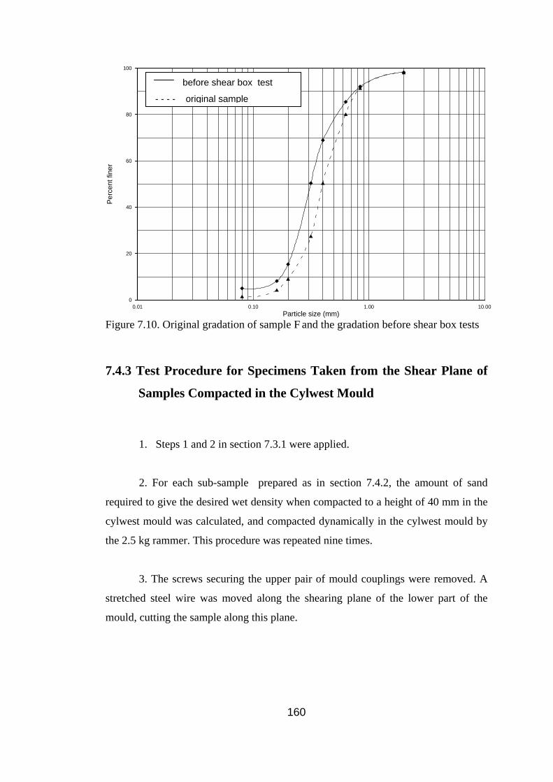
0.01 0.10 1.00 10.00Particle size (mm)
0
20
40
60
80
100
Perc
ent f
iner
before shear box test
- - - - original sample
Figure 7.10. Original gradation of sample F and the gradation before shear box tests 7.4.3 Test Procedure for Specimens Taken from the Shear Plane of
Samples Compacted in the Cylwest Mould
1. Steps 1 and 2 in section 7.3.1 were applied.
2. For each sub-sample prepared as in section 7.4.2, the amount of sand
required to give the desired wet density when compacted to a height of 40 mm in the
cylwest mould was calculated, and compacted dynamically in the cylwest mould by
the 2.5 kg rammer. This procedure was repeated nine times.
3. The screws securing the upper pair of mould couplings were removed. A
stretched steel wire was moved along the shearing plane of the lower part of the
mould, cutting the sample along this plane.
160

4. The lower half of the cylwest mould was placed on a wooden supporting
frame holding the shear surface in a horizontal position (Fig. 7.11). The core cutter,
of the right size for the shear box and carrying a label which enabled the direction of
shear in the shear box to be the same as in the cylwest, was placed on the shear
surface. Applying pressure through a wooden disc placed on top, the core cutter was
pressed manually into the sample in the cylwest mould until the top of the specimen
was flush with the top of the core cutter. The sand around the core cutter was
removed by means of a spatula, and the specimen cut at an adequate distance from
the cutting edge of the core cutter without disturbing the specimen.
5. The whole was turned up side down, and the upper end of the specimen
trimmed flush with the cutting edge of the core cutter. If the mass of the specimen
was less than the value calculated at (2), sand was added from the trimmings until the
desired mass was obtained. (The maximum amount needed to be added was 1 g to 2
g.)
6. The core cutter containing the specimen was held just above the shear box
according to the predefined direction of shear. The retaining plate together with the
porous stone and serrated grid plate (Fig. 7.2) were raised by pressing with the
fingers from below until the upper surface of the serrated plate touched the bottom of
the specimen. Then, the loading plate was placed on top of the specimen in the core
cutter and pushed slowly downwards while letting the retaining plate engage the pins
at the inner sides of the shear box.
7. After the specimen was placed in the shear box, the height of the specimen
was checked. If it was more than 20 mm, (the maximum height recorded at this stage
was 23 mm and in no case was this less than 20 mm) additional compaction was
applied to bring it down to 20 mm.
8. Steps 4 to 10 in section 7.3.1 were applied.
161
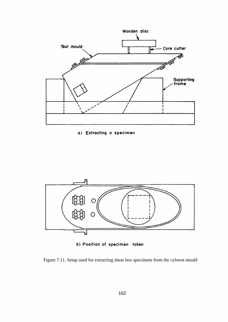
Wooden disc
Core cutter
Supporting frame
Test mould
a) Extracting a specimen
Figure 7.11. Setup used for extracting shear box specimens from the cylwest mould
162

9. For taking the second specimen, an additional wooden disc of height
50 mm was jacked into the bottom of the lower part of the cylwest mould thus
pushing the sample upwards by this amount. The protruding part of sample was
trimmed flush with the shear plane of the mould. A second shear box specimen was
taken as at step 4, and steps 5 to 8 were repeated.
10. Steps 1 to 9 were then repeated on the second sub-sample prepared as in
section 7.4.2.
7.4.4 Test Procedure for Specimens Taken from the Shear Plane of
Samples Compacted in the Priswest Mould
1. Steps 1 and 2 in section 7.3.1 were applied.
2. For each sub-sample prepared as in section 7.4.2, the mass of sand required
to give the desired wet density when compacted to a height of 51 mm in the
30-degree priswest mould was calculated, and compacted in this mould using the
Kango vibrating hammer, as in section 5.2.3. This procedure was repeated five times,
obtaining a compacted sample with the top about 10 mm above the top of the mould.
The collar was then removed, the surplus material scraped off, the surface smoothed,
and the lid screwed in position. The link bolts and spacers were removed. The
sample was cut by moving a stretched steel wire along the shearing surface of the
lower part of the mould.
3. The lower half of the priswest mould was held with the shear surface in a
horizontal position by using wooden blocks as in Fig. 7.12. A specimen was
extracted from position 1 (Fig. 7.12 (b)), following the same procedure as in section
7.4.3 (4).
163

Figure 7.12. Setup used for extracting shear box specimens from the priswest mould
a) Extracting a specimen
Test mould
Wooden block
b) Position of specimen taken
Wooden block
Wooden block
Position 1
Position 2
Wooden disc Core cutter
164
4. The steps 5 to 8 in section 7.4.3 were then applied to the specimen.
5. A second shear box specimen was taken as at step 3 from position 2
(Fig. 7.12 (b)), and steps 5 to 8 in section 7.4.3 were repeated
6. Steps 1 to 5 were then repeated on the sub-same sample prepared as in
section 7.4.2.
7.4.5 Results of Shear Box Tests on Specimens Taken from the Shear
Plane of Samples Compacted in the Cylwest and Priswest
Moulds
Ten shear box tests series SBC, SCC, SDC, SEC, SFC; SBP, SCP, SDP, SEP,
and SFP of four tests each were performed on the specimens taken from the cylwest
and priswest moulds. In this notation, the first letter signifies the shear box test; the
second letter denotes the sample tested; the C and P at the end denote the specimens
taken from the cylwest and priswest moulds respectively. The tests were evaluated
by using the computer program DIST02 (Mirata, 2002(b)). The results are
summarized in Tables 7.3 and 7.4 and plotted in Figs. 7.13 and 7.14.
165
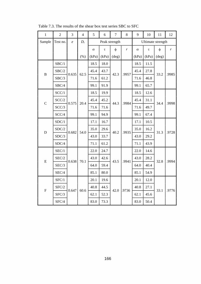
Table 7.3. The results of the shear box test series SBC to SFC
1 2 3 4 5 6 7 8 9 10 11 12
Peak strength Ultimate strength Dr
σ τ φ r σ τ φ r
Sample Test no. e
(%) (kPa) (kPa) (deg) (kPa) (kPa) (deg)
SBC/1 18.5 18.0 18.5 11.5
SBC/2 45.4 43.7 45.4 27.8
SBC/3 71.6 61.2 71.6 46.8 B
SBC/4
0.635 62.5
99.1 91.9
42.3 .9957
99.1 65.7
33.2 .9985
SCC/1 18.5 19.9 18.5 12.6
SCC/2 45.4 45.2 45.4 31.1
SCC/3 71.6 71.6 71.6 49.7 C
SCC/4
0.575 20.4
99.1 94.9
44.3 .9984
99.1 67.4
34.4 .9998
SDC/1 17.1 16.7 17.1 10.5
SDC/2 35.0 29.6 35.0 16.2
SDC/3 43.0 33.7 43.0 29.2 D
SDC/4
0.682 54.0
71.1 61.2
40.2 .9935
71.1 43.9
31.3 .9728
SEC/1 22.0 24.7 22.0 14.6
SEC/2 43.0 42.6 43.0 28.2
SEC/3 64.0 59.4 64.0 40.4 E
SEC/4
0.638 70.1
85.1 80.0
43.5 .9941
85.1 54.9
32.8 .9994
SFC/1 20.1 19.6 20.1 12.0
SFC/2 40.8 44.5 40.8 27.1
SFC/3 62.1 52.3 62.1 45.6 F
SFC/4
0.647 60.6
83.0 73.3
42.0 .9736
83.0 50.4
33.1 .9776
166
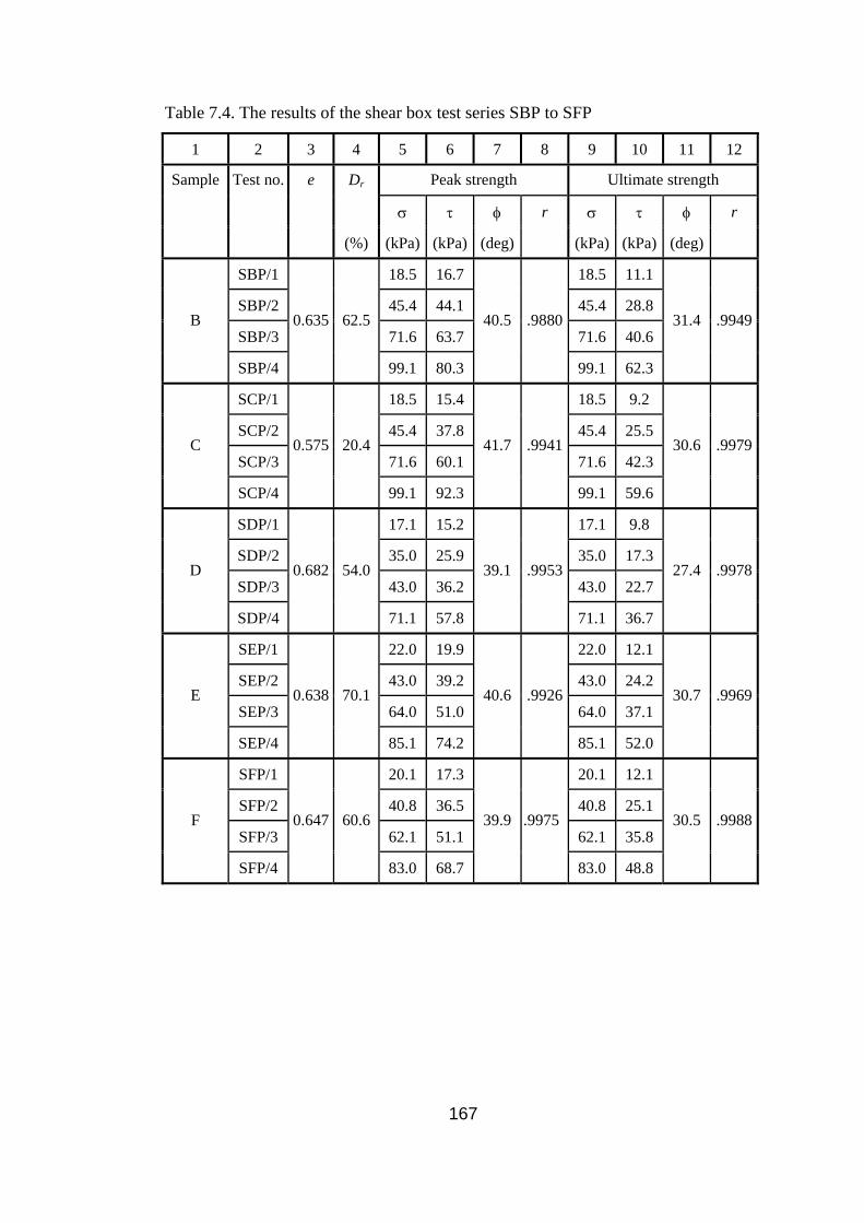
Table 7.4. The results of the shear box test series SBP to SFP
1 2 3 4 5 6 7 8 9 10 11 12
Peak strength Ultimate strength Dr
σ τ φ r σ τ φ r
Sample Test no. e
(%) (kPa) (kPa) (deg) (kPa) (kPa) (deg)
SBP/1 18.5 16.7 18.5 11.1
SBP/2 45.4 44.1 45.4 28.8
SBP/3 71.6 63.7 71.6 40.6 B
SBP/4
0.635 62.5
99.1 80.3
40.5 .9880
99.1 62.3
31.4 .9949
SCP/1 18.5 15.4 18.5 9.2
SCP/2 45.4 37.8 45.4 25.5
SCP/3 71.6 60.1 71.6 42.3 C
SCP/4
0.575 20.4
99.1 92.3
41.7 .9941
99.1 59.6
30.6 .9979
SDP/1 17.1 15.2 17.1 9.8
SDP/2 35.0 25.9 35.0 17.3
SDP/3 43.0 36.2 43.0 22.7 D
SDP/4
0.682 54.0
71.1 57.8
39.1 .9953
71.1 36.7
27.4 .9978
SEP/1 22.0 19.9 22.0 12.1
SEP/2 43.0 39.2 43.0 24.2
SEP/3 64.0 51.0 64.0 37.1 E
SEP/4
0.638 70.1
85.1 74.2
40.6 .9926
85.1 52.0
30.7 .9969
SFP/1 20.1 17.3 20.1 12.1
SFP/2 40.8 36.5 40.8 25.1
SFP/3 62.1 51.1 62.1 35.8 F
SFP/4
0.647 60.6
83.0 68.7
39.9 .9975
83.0 48.8
30.5 .9988
167

0 25 50 75 100 1Normal stress (kPa)
25 0 25 50 75 100Normal stress (kPa)
1250
25
50
75
100
125
Shea
r stre
ngth
(kPa
)
0 25 50 75 100 0 25 50 75 100Normal stress (kPa)
1250
25
50
75
100
125
Shea
r stre
ngth
(kPa
)
0 25 50 75 100Normal stress (kPa)
1250
25
50
75
100
125
Shea
r stre
ngth
(kPa
)
0
25
50
75
100
125
Shea
r stre
ngth
(kPa
)
(a) Series SBC (b) Series SCC
Normal stress (kPa)
0
25
50
75
100
Shea
r stre
ngth
(kPa
)
(c) Series SDC (d) Series SEC
(e) Series SFC
υ υ at peak σ σ at ultimate
Figure 7.13. The results of shear box tests on specimens taken from the shear plane
of cylwest samples
168
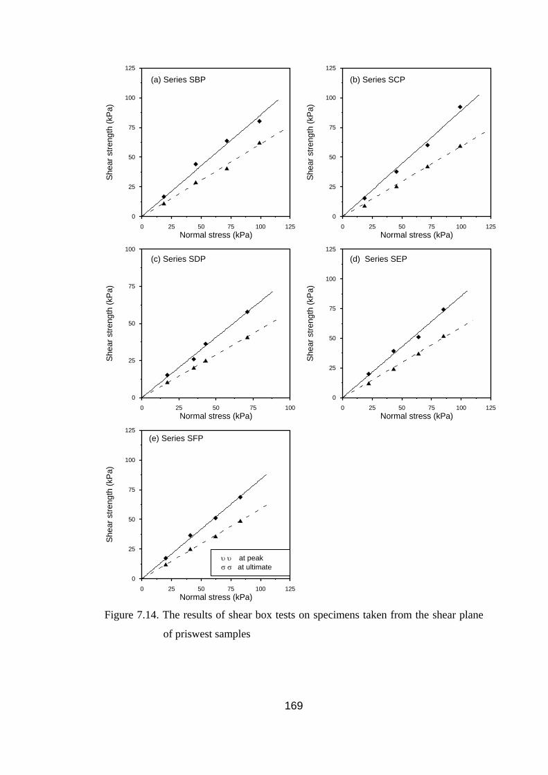
0 25 50 75 100 1Normal stress (kPa)
25 0 25 50 75 100Normal stress (kPa)
1250
25
50
75
100
125
Shea
r stre
ngth
(kPa
)
0 25 50 75 100 0 25 50 75 100Normal stress (kPa)
1250
25
50
75
100
125
Shea
r stre
ngth
(kPa
)
0 25 50 75 100Normal stress (kPa)
1250
25
50
75
100
125
Shea
r stre
ngth
(kPa
)
0
25
50
75
100
125
Shea
r stre
ngth
(kPa
)
(a) Series SBP (b) Series SCP
Normal stress (kPa)
0
25
50
75
100
Shea
r stre
ngth
(kPa
)
(c) Series SDP (d) Series SEP
(e) Series SFP
υ υ at peak σ σ at ultimate
Figure 7.14. The results of shear box tests on specimens taken from the shear plane
of priswest samples
169
CHAPTER 8
DISCUSSIONS
8.1 Discussion of Shear Test Results
The paragraphs in the following sub-sections have been numbered for ease of
reference.
8.1.1 Shear Strength Measured in Wedge Shear and Triaxial Tests
1. The summary of cylwests, priswests, and triaxial tests performed on
samples A to F at the lower density under the lower and higher ranges of normal
stress σ are given in Table 8.1. The corresponding results for samples D to F at the
higher density are given in Table 8.2. All peak friction angles measured for each
sample are compared in Table 8.3. In this table, for both densities, φc denotes values
obtained from cylwests under the lower ranges of σ; φpl and φtl denote those from the
results of priswests and triaxial tests under the lower ranges of σ respectively; φph
and φth denote those from the results of priswests and triaxial tests under the higher
ranges of σ respectively; φpa and φta denote those from the combined results of all
priswests and triaxial tests respectively. These results, however, are affected by
different degrees of previous particle crushing in specimens used for some of the
tests (Tables 5.1, 5.8, and 6.1). To eliminate the effect of particle crushing, bar chart
comparisons have been given between the results of tests performed on identical
specimens regarding previous use in shear tests. Thus the comparisons in Figs. 8.1 to
8.3 are those of tests on previously untested specimens; the comparisons in Figs. 8.4
170
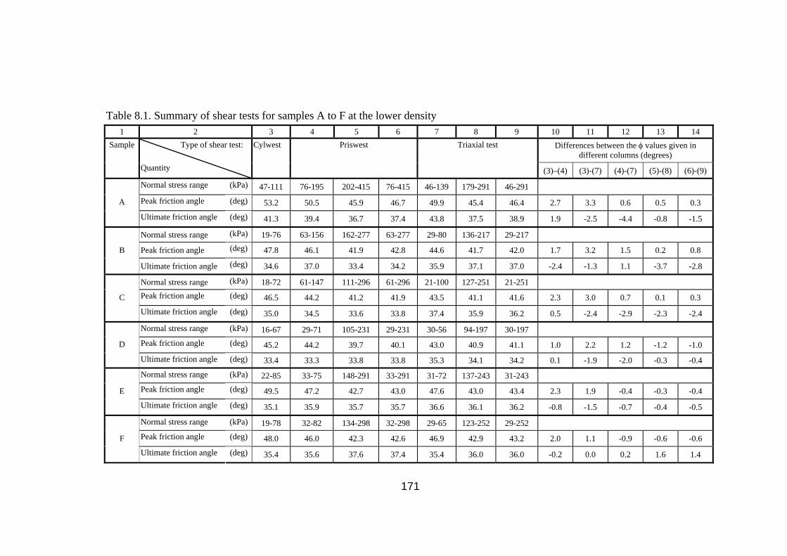
Table 8.1. Summary of shear tests for samples A to F at the lower density 1 2 3 4 5 6 7 8 9 10 11 12 13 14
Differences between the φ values given in different columns (degrees)
Sample Type of shear test: Quantity
Cylwest
Priswest Triaxial test
(3)–(4) (3)-(7) (4)-(7) (5)-(8) (6)-(9)
Normal stress range (kPa) 47-111 76-195 202-415 76-415 46-139 179-291 46-291
Peak friction angle (deg) 53.2 50.5 45.9 46.7 49.9 45.4 46.4 2.7 3.3 0.6 0.5 0.3A
Ultimate friction angle (deg) 41.3 39.4 36.7 37.4 43.8 37.5 38.9 1.9 -2.5 -4.4 -0.8 -1.5
Normal stress range (kPa) 19-76 63-156 162-277 63-277 29-80 136-217 29-217
Peak friction angle (deg) 47.8 46.1 41.9 42.8 44.6 41.7 42.0 1.7 3.2 1.5 0.2 0.8B
Ultimate friction angle (deg) 34.6 37.0 33.4 34.2 35.9 37.1 37.0 -2.4 -1.3 1.1 -3.7 -2.8
Normal stress range (kPa) 18-72 61-147 111-296 61-296 21-100 127-251 21-251Peak friction angle (deg) 46.5 44.2 41.2 41.9 43.5 41.1 41.6 2.3 3.0 0.7 0.1 0.3C
Ultimate friction angle (deg) 35.0 34.5 33.6 33.8 37.4 35.9 36.2 0.5 -2.4 -2.9 -2.3 -2.4
Normal stress range (kPa) 16-67 29-71 105-231 29-231 30-56 94-197 30-197Peak friction angle (deg) 45.2 44.2 39.7 40.1 43.0 40.9 41.1 1.0 2.2 1.2 -1.2 -1.0D
Ultimate friction angle (deg) 33.4 33.3 33.8 33.8 35.3 34.1 34.2 0.1 -1.9 -2.0 -0.3 -0.4
Normal stress range (kPa) 22-85 33-75 148-291 33-291 31-72 137-243 31-243Peak friction angle (deg) 49.5 47.2 42.7 43.0 47.6 43.0 43.4 2.3 1.9 -0.4 -0.3 -0.4E
Ultimate friction angle (deg) 35.1 35.9 35.7 35.7 36.6 36.1 36.2 -0.8 -1.5 -0.7 -0.4 -0.5
Normal stress range (kPa) 19-78 32-82 134-298 32-298 29-65 123-252 29-252Peak friction angle (deg) 48.0 46.0 42.3 42.6 46.9 42.9 43.2 2.0 1.1 -0.9 -0.6 -0.6F
Ultimate friction angle (deg) 35.4 35.6 37.6 37.4 35.4 36.0 36.0 -0.2 0.0 0.2 1.6 1.4
171

Table 8.2. Summary of shear tests for samples D to F at the higher density 1 2 3 4 5 6 7 8 9 10 11 12 13 14
Differences between the φ values given in different columns (degrees)
Sample Type of shear test: Quantity
Cylwest
Priswest Triaxial test
(3)–(4) (3)-(7) (4)-(7) (5)-(8) (6)-(9)Normal stress range (kPa) 23-79 33-77 181-303 33-303 29-84 166-254 29-254Peak friction angle (deg) 48.5 45.0 42.9 43.0 45.9 43.6 43.8 3.5 2.6 -0.9 -0.7 -0.8D
Ultimate friction angle (deg) 33.8 34.5 32.7 32.8 34.4 35.2 35.2 -0.7 -0.6 0.1 -2.5 -2.4
Normal stress range (kPa) 53-108 39-105 199-329 39-329 42-88 188-282 42-282
Peak friction angle (deg) 53.5 47.7 43.8 44.2 50.9 45.7 46.2 5.8 2.6 -3.2 -1.9 -2.0E
Ultimate friction angle (deg) 36.4 35.6 35.4 35.4 36.8 38.3 38.2 0.8 -0.4 -1.2 -2.9 -2.8
Normal stress range (kPa) 42-103 41-87 186-323 41-323 38-85 176-272 38-272Peak friction angle (deg) 52.4 46.7 43.1 43.4 50.3 44.3 44.9 5.7 2.1 -3.5 -1.2 -1.5F
Ultimate friction angle (deg) 35.5 34.9 34.6 34.6 35.1 39.7 39.5 0.6 0.4 -0.2 -5.1 -4.9
172

Table 8.3. Peak friction angles obtained from the cylwests, priswests, and triaxial tests for samples A to F 1 2 3 4 5 6 7 8 9 10 11 12 13 14 15 16 17 18 19 20 21 22 23 24 25
Peak friction angles at the lower density (degrees)
Peak friction angles at the higher density (degrees)
Differences between the values of peak friction angles
given in different columns (degrees)
Sample
φc
φpl
φph
φpa
φtl
φth
φta
φc
φpl
φph
φpa
φtl
φth
φta
(2) – (3) (2) – (6) (3) – (6) (4) – (7) (5) – (8) (9) – (10) (9) – (13) (10) – (13) (11) – (14) (12) – (15)
A 53.2 50.5 45.9 46.7 49.9 45.4 46.4 … … … … … … … 2.7 3.3 0.6 0.5 0.3 … … … … …
B 47.8 46.1 41.9 42.8 44.6 41.7 42.0 … … … … … … … 1.7 3.2 1.5 0.2 0.8 … … … … …
C 46.5 44.2 41.2 41.9 43.5 41.1 41.6 … … … … … … … 2.3 3.0 0.7 0.1 0.3 … … … … …
D 45.2 44.2 39.7 40.1 43.0 40.9 41.1 48.5 45.0 42.9 43.0 45.9 43.6 43.8 1.0 2.2 1.2 -1.2 -1.0 3.5 2.6 -0.9 -0.7 -0.8
E 49.5 47.2 42.7 43.0 47.6 43.0 43.4 53.5 47.7 43.8 44.2 50.9 45.7 46.2 2.3 1.9 -0.4 -0.3 -0.4 5.8 2.6 -3.2 -1.9 -2.0
F 48.0 46.0 42.3 42.6 46.9 42.9 43.2 52.4 46.7 43.1 43.4 50.3 44.3 44.9 2.0 1.1 -0.9 -0.6 -0.6 5.7 2.1 -3.5 -1.2 -1.5
173
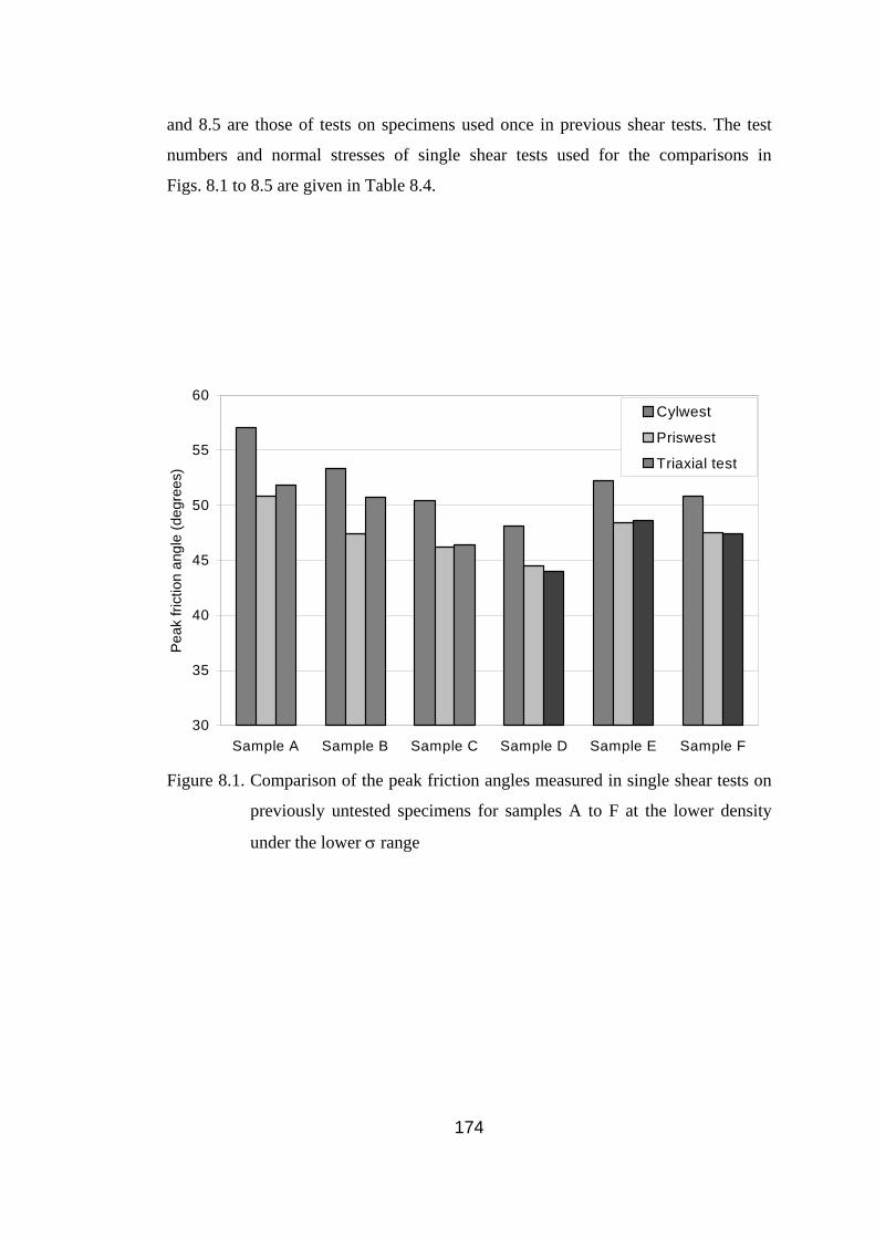
and 8.5 are those of tests on specimens used once in previous shear tests. The test
numbers and normal stresses of single shear tests used for the comparisons in
Figs. 8.1 to 8.5 are given in Table 8.4.
30
35
40
45
50
55
60
Sample A Sample B Sample C Sample D Sample E Sample F
Pea
k fri
ctio
n an
gle
(deg
rees
)
Cylwest
Priswest
Triaxial test
Figure 8.1. Comparison of the peak friction angles measured in single shear tests on
previously untested specimens for samples A to F at the lower density
under the lower σ range
174

35
40
45
50
Sample A Sample B
Pea
k fri
ctio
n an
gle
(deg
rees
)P riswest
Triaxial test
Figure 8.2. Comparison of the peak friction angles measured in single shear tests on
previously untested specimens for samples A and B at the lower density
under the higher σ range
3 0
3 5
4 0
4 5
5 0
5 5
6 0
S a m p le D S a m p le E S a m p le F
Pea
k fri
ctio
n an
gle
(deg
rees
)
C y lw e s t
P r is w e s t
T r ia x ia l te s t
Figure 8.3. Comparison of the peak friction angles measured in single shear tests on
previously untested specimens for samples D to F at the higher density
under the lower σ range
175
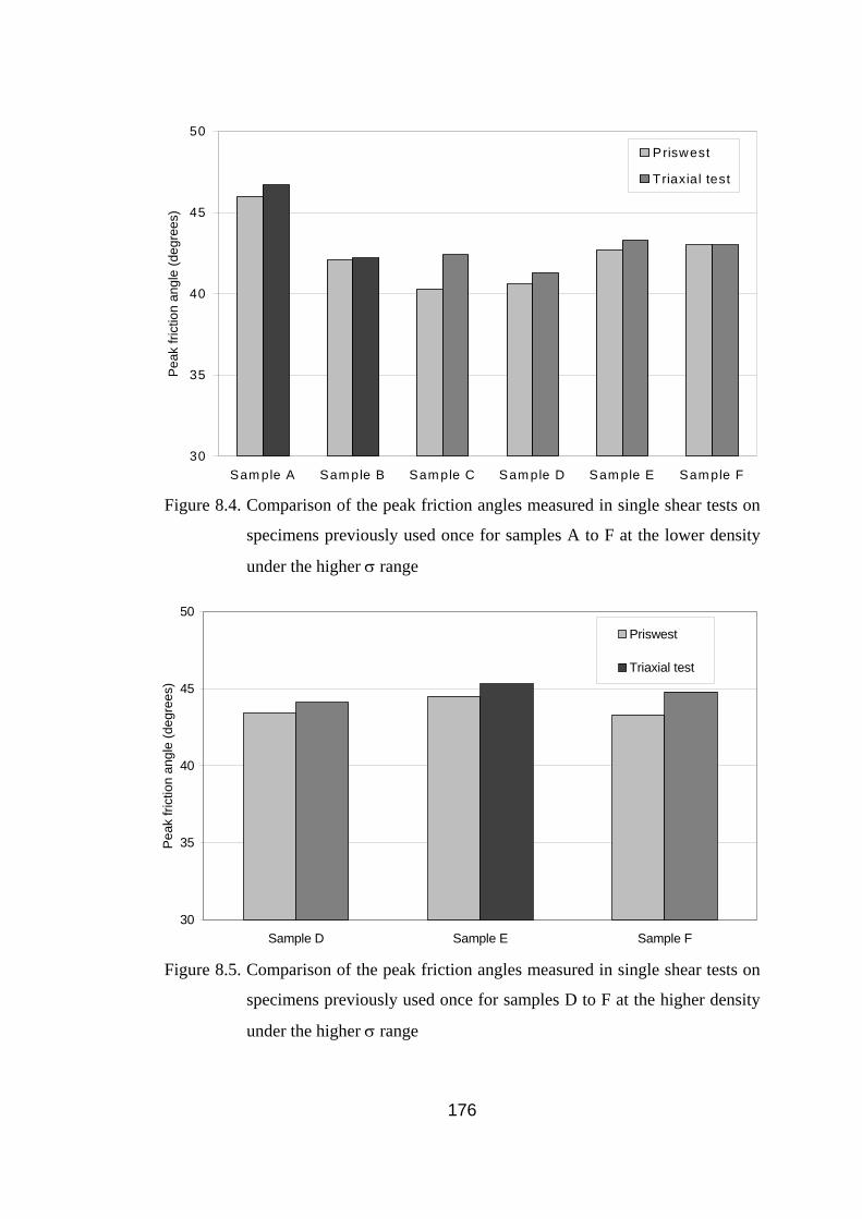
30
35
40
45
50
Sam ple A Sam ple B Sam ple C Sam ple D Sam ple E Sam ple F
Pea
k fri
ctio
n an
gle
(deg
rees
)P riswest
Triaxial test
Figure 8.4. Comparison of the peak friction angles measured in single shear tests on
specimens previously used once for samples A to F at the lower density
under the higher σ range
30
35
40
45
50
Sample D Sample E Sample F
Pea
k fri
ctio
n an
gle
(deg
rees
)
Priswest
Triaxial test
Figure 8.5. Comparison of the peak friction angles measured in single shear tests on
specimens previously used once for samples D to F at the higher density
under the higher σ range
176

Table 8.4. Test numbers and normal stresses of single shear tests used for the
comparisons in Figs. 8.1 to 8.5
1 2 3 4 5 6 7 8
Cylwest Priswest Triaxial test
Test σ Test σ Test σ
Figure
no.
Sample
no.* (kPa) no.# (kPa) no.$ (kPa)
A CA/3 47.1 PA1/1 76.5 TA/1 46.2
B CB/1 23.0 PB1/1 63.7 TB/1 28.7
C CC/1 19.6 PC1/1 60.7 TC/1 20.6
D CD/3 17.2 PD1/1 29.5 TD/1 30.5
E CE/1 24.6 PE1/1 33.5 TE/1 31.4
8.1
F CF/3 21.1 PF1/1 32.4 TF/1 28.8
A ... ... PA2/1 202.1 TA/5 179.1 8.2
B ... ... PB2/1 161.6 TB/5 136.1
D CDH/1 23.8 PDH1/1 33.4 TDH/1 28.7
E CEH/3 58.6 PEH1/1 39.7 TEH/1 42.3 8.3
F CFH/1 42.4 PFH1/1 41.9 TFH/1 38.4
A ... ... PA2/2 355.7 TA/6 242.2
B ... ... PB2/2 214.0 TB/6 182.9
C ... ... PC2/2 187.5 TC/6 163.8
D ... ... PD2/2 184.8 TD/6 165.3
E ... ... PE2/2 221.5 TE/6 193.0
8.4
F ... ... PF2/2 232.6 TF/6 203.7
D ... ... PDH2/2 241.6 TDH/5 214.9
E ... ... PEH2/2 275.5 TEH/5 241.8 8.5
F ... ... PFH2/2 244.6 TFH/5 217.7
* Tables 5.5 to 5.7 # Tables 5.15 to 5.19 $ Tables 6.2 to 6.10
177
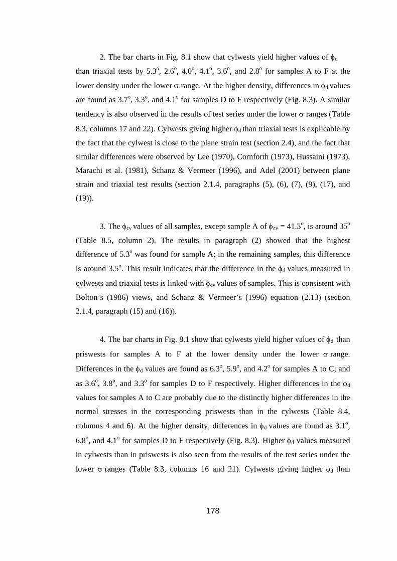
2. The bar charts in Fig. 8.1 show that cylwests yield higher values of φd
than triaxial tests by 5.3o, 2.6o, 4.0o, 4.1o, 3.6o, and 2.8o for samples A to F at the
lower density under the lower σ range. At the higher density, differences in φd values
are found as 3.7o, 3.3o, and 4.1o for samples D to F respectively (Fig. 8.3). A similar
tendency is also observed in the results of test series under the lower σ ranges (Table
8.3, columns 17 and 22). Cylwests giving higher φd than triaxial tests is explicable by
the fact that the cylwest is close to the plane strain test (section 2.4), and the fact that
similar differences were observed by Lee (1970), Cornforth (1973), Hussaini (1973),
Marachi et al. (1981), Schanz & Vermeer (1996), and Adel (2001) between plane
strain and triaxial test results (section 2.1.4, paragraphs (5), (6), (7), (9), (17), and
(19)).
3. The φcv values of all samples, except sample A of φcv = 41.3o, is around 35o
(Table 8.5, column 2). The results in paragraph (2) showed that the highest
difference of 5.3o was found for sample A; in the remaining samples, this difference
is around 3.5o. This result indicates that the difference in the φd values measured in
cylwests and triaxial tests is linked with φcv values of samples. This is consistent with
Bolton’s (1986) views, and Schanz & Vermeer’s (1996) equation (2.13) (section
2.1.4, paragraph (15) and (16)).
4. The bar charts in Fig. 8.1 show that cylwests yield higher values of φd than
priswests for samples A to F at the lower density under the lower σ range.
Differences in the φd values are found as 6.3o, 5.9o, and 4.2o for samples A to C; and
as 3.6o, 3.8o, and 3.3o for samples D to F respectively. Higher differences in the φd
values for samples A to C are probably due to the distinctly higher differences in the
normal stresses in the corresponding priswests than in the cylwests (Table 8.4,
columns 4 and 6). At the higher density, differences in φd values are found as 3.1o,
6.8o, and 4.1o for samples D to F respectively (Fig. 8.3). Higher φd values measured
in cylwests than in priswests is also seen from the results of the test series under the
lower σ ranges (Table 8.3, columns 16 and 21). Cylwests giving higher φd than
178
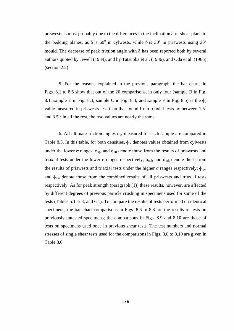
priswests is most probably due to the differences in the inclination δ of shear plane to
the bedding planes, as δ is 60o in cylwests, while δ is 30o in priswests using 30o
mould. The decrease of peak friction angle with δ has been reported both by several
authors quoted by Jewell (1989), and by Tatsuoka et al. (1986), and Oda et al. (1986)
(section 2.2).
5. For the reasons explained in the previous paragraph, the bar charts in
Figs. 8.1 to 8.5 show that out of the 20 comparisons, in only four (sample B in Fig.
8.1, sample E in Fig. 8.3, sample C in Fig. 8.4, and sample F in Fig. 8.5) is the φd
value measured in priswests less than that found from triaxial tests by between 1.5o
and 3.5o; in all the rest, the two values are nearly the same.
6. All ultimate friction angles φcv measured for each sample are compared in
Table 8.5. In this table, for both densities, φuc denotes values obtained from cylwests
under the lower σ ranges; φupl and φutl denote those from the results of priswests and
triaxial tests under the lower σ ranges respectively; φuph and φuth denote those from
the results of priswests and triaxial tests under the higher σ ranges respectively; φupa
and φuta denote those from the combined results of all priswests and triaxial tests
respectively. As for peak strength (paragraph (1)) these results, however, are affected
by different degrees of previous particle crushing in specimens used for some of the
tests (Tables 5.1, 5.8, and 6.1). To compare the results of tests performed on identical
specimens, the bar chart comparisons in Figs. 8.6 to 8.8 are the results of tests on
previously untested specimens; the comparisons in Figs. 8.9 and 8.10 are those of
tests on specimens used once in previous shear tests. The test numbers and normal
stresses of single shear tests used for the comparisons in Figs. 8.6 to 8.10 are given in
Table 8.6.
179
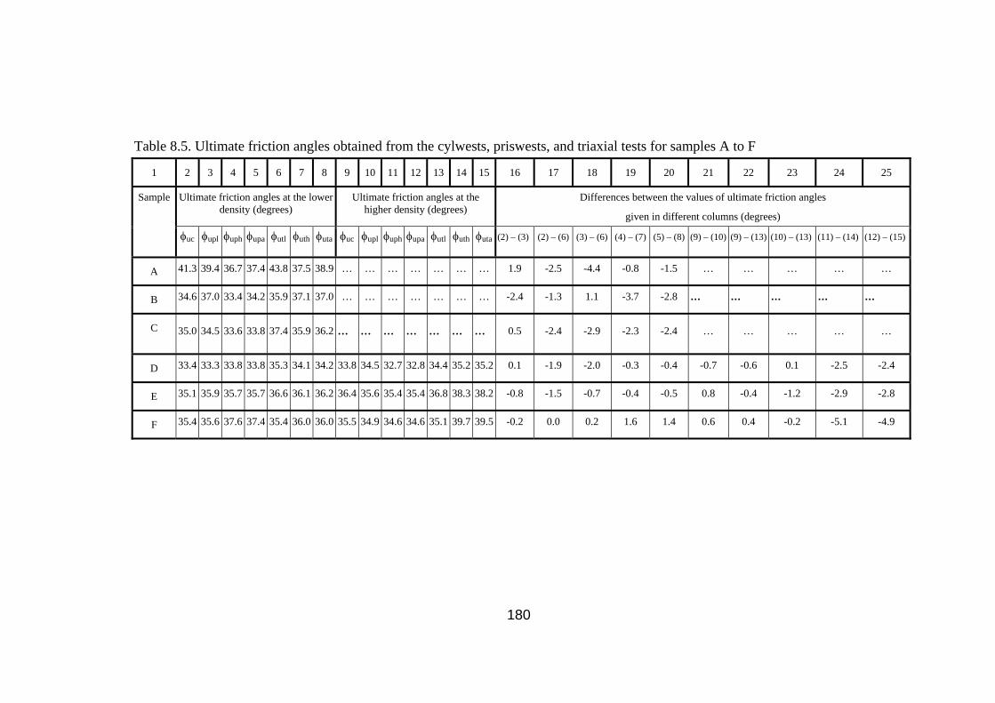
Table 8.5. Ultimate friction angles obtained from the cylwests, priswests, and triaxial tests for samples A to F
1 2 3 4 5 6 7 8 9 10 11 12 13 14 15 16 17 18 19 20 21 22 23 24 25
Ultimate friction angles at the lower density (degrees)
Ultimate friction angles at the higher density (degrees)
Differences between the values of ultimate friction angles
given in different columns (degrees)
Sample
φuc
φupl
φuph
φupa
φutl
φuth
φuta
φuc
φupl
φuph
φupa
φutl
φuth
φuta
(2) – (3) (2) – (6) (3) – (6) (4) – (7) (5) – (8) (9) – (10) (9) – (13) (10) – (13) (11) – (14) (12) – (15)
A 41.3 39.4 36.7 37.4 43.8 37.5 38.9 … … … … … … … 1.9 -2.5 -4.4 -0.8 -1.5 … … … … …
B 34.6 37.0 33.4 34.2 35.9 37.1 37.0 … … … … … … … -2.4 -1.3 1.1 -3.7 -2.8 … … … … …
C 35.0 34.5 33.6 33.8 37.4 35.9 36.2 … … … … … … … 0.5 -2.4 -2.9 -2.3 -2.4 … … … … …
D 33.4 33.3 33.8 33.8 35.3 34.1 34.2 33.8 34.5 32.7 32.8 34.4 35.2 35.2 0.1 -1.9 -2.0 -0.3 -0.4 -0.7 -0.6 0.1 -2.5 -2.4
E 35.1 35.9 35.7 35.7 36.6 36.1 36.2 36.4 35.6 35.4 35.4 36.8 38.3 38.2 -0.8 -1.5 -0.7 -0.4 -0.5 0.8 -0.4 -1.2 -2.9 -2.8
F 35.4 35.6 37.6 37.4 35.4 36.0 36.0 35.5 34.9 34.6 34.6 35.1 39.7 39.5 -0.2 0.0 0.2 1.6 1.4 0.6 0.4 -0.2 -5.1 -4.9
180

25
30
35
40
45
50
S am ple A Sam ple B S am ple C S am ple D S am ple E S am ple F
Ulti
mat
e fri
ctio
n an
gle
(deg
rees
)
C ylwest
P riswest
T riaxia l test
Figure 8.6. Comparison of the ultimate friction angles measured in single shear tests
on previously untested specimens for samples A to F at the lower density
under the lower σ range
25
30
35
40
45
Sample A Sample B
Ulti
mat
e fri
ctio
n an
gle
(deg
rees
)
P riswest
Triaxial test
Figure 8.7. Comparison of the ultimate friction angles measured in single shear tests
on previously untested specimens for samples A and B at the lower
density under the higher σ range
181

2 5
3 0
3 5
4 0
S a m p le D S a m p le E S a m p le F
Ulti
mat
e fri
ctio
n an
gle
(deg
rees
)
C y lw e s t
P risw e s t
T ria x ia l te s t
Figure 8.8. Comparison of the ultimate friction angles measured in single shear tests
on previously untested specimens for samples D to F at the higher
density under the lower σ range
25
30
35
40
Sample A Sample B Sample C Sample D Sample E Sample F
Ulti
mat
e fri
ctio
n an
gle
(deg
rees
)
Priswest
Triaxial test
Figure 8.9. Comparison of the ultimate friction angles measured in single shear tests
on specimens previously used once for samples A to F at the lower
density under the higher σ range
182
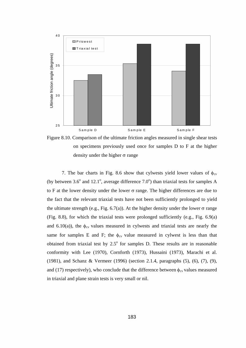
2 5
3 0
3 5
4 0
S a m p le D S a m p le E S a m p le F
Ulti
mat
e fri
ctio
n an
gle
(deg
rees
)
P r is w e s t
T r ia x ia l te s t
Figure 8.10. Comparison of the ultimate friction angles measured in single shear tests
on specimens previously used once for samples D to F at the higher
density under the higher σ range
7. The bar charts in Fig. 8.6 show that cylwests yield lower values of φcv
(by between 3.6o and 12.1o, average difference 7.0o) than triaxial tests for samples A
to F at the lower density under the lower σ range. The higher differences are due to
the fact that the relevant triaxial tests have not been sufficiently prolonged to yield
the ultimate strength (e.g., Fig. 6.7(a)). At the higher density under the lower σ range
(Fig. 8.8), for which the triaxial tests were prolonged sufficiently (e.g., Fig. 6.9(a)
and 6.10(a)), the φcv values measured in cylwests and triaxial tests are nearly the
same for samples E and F; the φcv value measured in cylwest is less than that
obtained from triaxial test by 2.5o for samples D. These results are in reasonable
conformity with Lee (1970), Cornforth (1973), Hussaini (1973), Marachi et al.
(1981), and Schanz & Vermeer (1996) (section 2.1.4, paragraphs (5), (6), (7), (9),
and (17) respectively), who conclude that the difference between φcv values measured
in triaxial and plane strain tests is very small or nil.
183

Table 8.6. Test numbers and normal stresses of single shear tests used for the
comparisons in Figs. 8.6 to 8.10
1 2 3 4 5 6 7 8
Cylwest Priswest Triaxial test
Test σ Test σ Test σ
Figure
no.
Sample
no.* (kPa) no.# (kPa) no.$ (kPa)
A CA/1 65.5 PA1/1 93.8 TA/1 45.0
B CB/1 29.8 PB1/1 89.8 TB/1 27.7
C CC/3 19.5 PC1/1 83.1 TC/1 19.8
D CD/3 18.7 PD1/1 35.1 TD/1 28.3
E CE/3 25.6 PE1/1 37.6 TE/1 29.3
8.6
F CF/3 23.0 PF1/1 37.2 TF/1 26.4
A ... ... PA2/1 178.2 TA/5 169.4 8.7
B ... ... PB2/1 198.3 TB/5 126.3
D CDH/1 23.4 PDH1/1 31.9 TDH/1 27.2
E CEH/3 58.1 PEH1/1 47.6 TEH/1 36.0 8.8
F CFH/1 44.6 PFH1/1 54.0 TFH/1 34.5
A ... ... PA2/2 276.1 TA/6 224.8
B ... ... PB2/2 260.4 TB/6 176.1
C ... ... PC2/2 224.1 TC/6 155.0
D ... ... PD2/2 201.1 TD/6 153.7
E ... ... PE2/2 218.3 TE/6 185.5
8.9
F ... ... PF2/2 214.4 TF/6 190.7
D ... ... PDH2/2 284.0 TDH/5 192.4
E ... ... PEH2/2 328.8 TEH/5 232.4 8.10
F ... ... PFH2/2 268.8 TFH/5 202.5
* Tables 5.5 to 5.7 # Tables 5.15 to 5.19 $ Tables 6.2 to 6.10
184
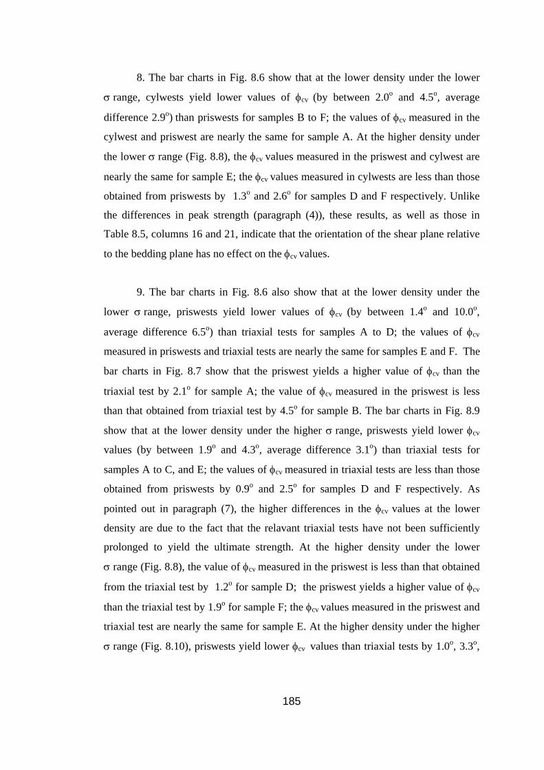
8. The bar charts in Fig. 8.6 show that at the lower density under the lower
σ range, cylwests yield lower values of φcv (by between 2.0o and 4.5o, average
difference 2.9o) than priswests for samples B to F; the values of φcv measured in the
cylwest and priswest are nearly the same for sample A. At the higher density under
the lower σ range (Fig. 8.8), the φcv values measured in the priswest and cylwest are
nearly the same for sample E; the φcv values measured in cylwests are less than those
obtained from priswests by 1.3o and 2.6o for samples D and F respectively. Unlike
the differences in peak strength (paragraph (4)), these results, as well as those in
Table 8.5, columns 16 and 21, indicate that the orientation of the shear plane relative
to the bedding plane has no effect on the φcv values.
9. The bar charts in Fig. 8.6 also show that at the lower density under the
lower σ range, priswests yield lower values of φcv (by between 1.4o and 10.0o,
average difference 6.5o) than triaxial tests for samples A to D; the values of φcv
measured in priswests and triaxial tests are nearly the same for samples E and F. The
bar charts in Fig. 8.7 show that the priswest yields a higher value of φcv than the
triaxial test by 2.1o for sample A; the value of φcv measured in the priswest is less
than that obtained from triaxial test by 4.5o for sample B. The bar charts in Fig. 8.9
show that at the lower density under the higher σ range, priswests yield lower φcv
values (by between 1.9o and 4.3o, average difference 3.1o) than triaxial tests for
samples A to C, and E; the values of φcv measured in triaxial tests are less than those
obtained from priswests by 0.9o and 2.5o for samples D and F respectively. As
pointed out in paragraph (7), the higher differences in the φcv values at the lower
density are due to the fact that the relavant triaxial tests have not been sufficiently
prolonged to yield the ultimate strength. At the higher density under the lower
σ range (Fig. 8.8), the value of φcv measured in the priswest is less than that obtained
from the triaxial test by 1.2o for sample D; the priswest yields a higher value of φcv
than the triaxial test by 1.9o for sample F; the φcv values measured in the priswest and
triaxial test are nearly the same for sample E. At the higher density under the higher
σ range (Fig. 8.10), priswests yield lower φcv values than triaxial tests by 1.0o, 3.3o,
185
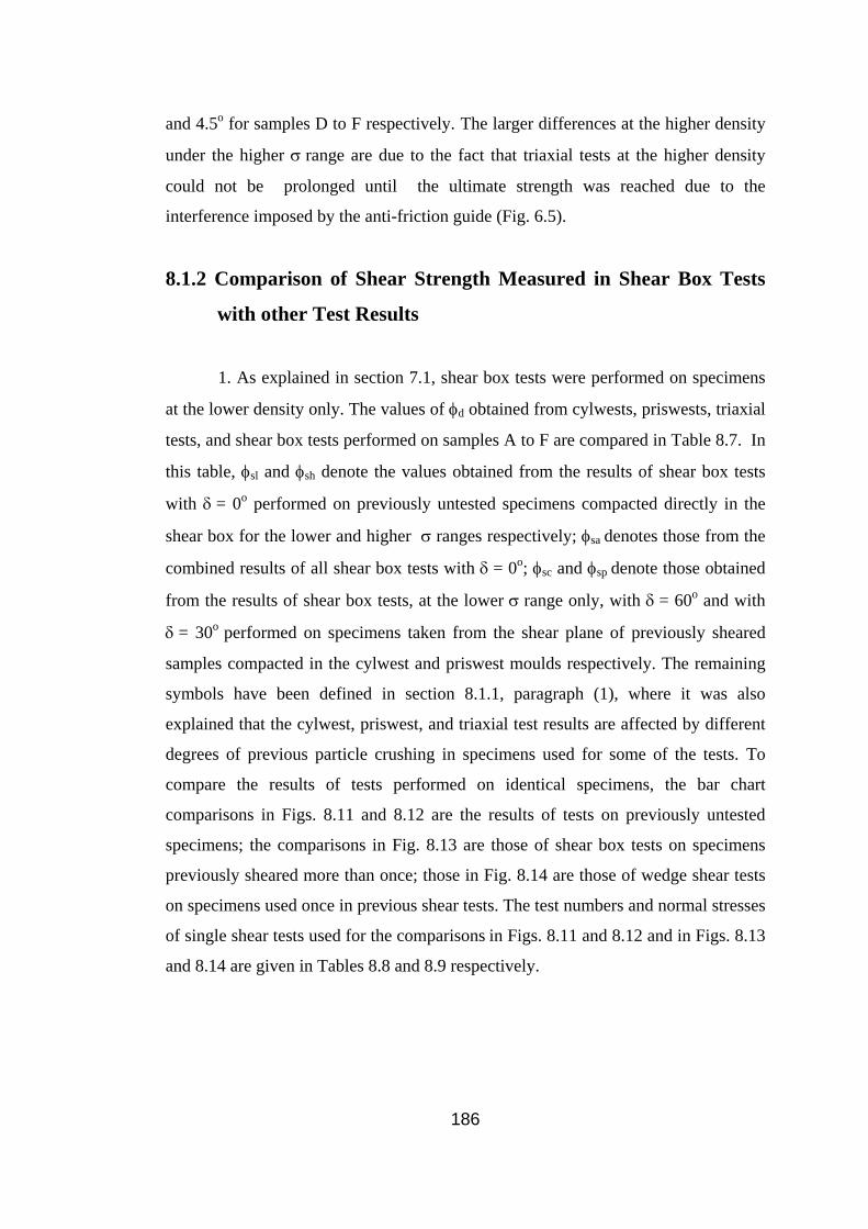
and 4.5o for samples D to F respectively. The larger differences at the higher density
under the higher σ range are due to the fact that triaxial tests at the higher density
could not be prolonged until the ultimate strength was reached due to the
interference imposed by the anti-friction guide (Fig. 6.5).
8.1.2 Comparison of Shear Strength Measured in Shear Box Tests
with other Test Results
1. As explained in section 7.1, shear box tests were performed on specimens
at the lower density only. The values of φd obtained from cylwests, priswests, triaxial
tests, and shear box tests performed on samples A to F are compared in Table 8.7. In
this table, φsl and φsh denote the values obtained from the results of shear box tests
with δ = 0o performed on previously untested specimens compacted directly in the
shear box for the lower and higher σ ranges respectively; φsa denotes those from the
combined results of all shear box tests with δ = 0o; φsc and φsp denote those obtained
from the results of shear box tests, at the lower σ range only, with δ = 60o and with
δ = 30o performed on specimens taken from the shear plane of previously sheared
samples compacted in the cylwest and priswest moulds respectively. The remaining
symbols have been defined in section 8.1.1, paragraph (1), where it was also
explained that the cylwest, priswest, and triaxial test results are affected by different
degrees of previous particle crushing in specimens used for some of the tests. To
compare the results of tests performed on identical specimens, the bar chart
comparisons in Figs. 8.11 and 8.12 are the results of tests on previously untested
specimens; the comparisons in Fig. 8.13 are those of shear box tests on specimens
previously sheared more than once; those in Fig. 8.14 are those of wedge shear tests
on specimens used once in previous shear tests. The test numbers and normal stresses
of single shear tests used for the comparisons in Figs. 8.11 and 8.12 and in Figs. 8.13
and 8.14 are given in Tables 8.8 and 8.9 respectively.
186

Table 8.7. Peak friction angles obtained from cylwests, priswests, triaxial tests, and shear box tests for samples A to F at the lower density
1 2 3 4 5 6 7 8 9 10 11 12 13 14 15 16 17 18 19 20 21 22
Peak friction angles
(degrees)
Differences between the values of peak friction angles given in different columns
(degrees)
Sample
φc φpl φph φpa φtl φth φta φsl φsh φsa φsc φsp (2) - (9) (3) - (9) (6) – (9) (4) – (10) (7) – (10) (5) – (11) (8) – (11) (2) – (3) (12) – 13)
A 53.2 50.5 45.9 46.7 49.9 45.4 46.4 45.5 41.8 42.1 … … 7.7 5.0 4.4 4.1 3.6 4.6 4.3 2.7 ...
B 47.8 46.1 41.9 42.8 44.6 41.7 42.0 42.7 40.1 40.4 42.3 40.5 5.1 3.4 1.9 1.8 1.6 2.4 1.6 1.7 1.8
C 46.5 44.2 41.2 41.9 43.5 41.1 41.6 41.1 39.2 39.4 44.3 41.7 5.4 3.1 2.4 2.0 1.9 2.5 2.2 2.3 2.6
D 45.2 44.2 39.7 40.1 43.0 40.9 41.1 38.6 36.6 36.8 40.2 39.0 6.6 5.6 4.4 3.1 4.3 3.3 4.3 1.0 1.2
E 49.5 47.2 42.7 43.0 47.6 43.0 43.4 40.5 37.6 37.8 43.5 40.6 9.0 6.7 7.1 5.1 5.4 5.2 5.6 2.3 2.9
F 48.0 46.0 42.3 42.6 46.9 42.9 43.2 40.5 38.3 38.5 42.0 39.9 7.5 5.5 6.4 4.0 4.6 4.1 4.7 2.0 2.1
187
30
35
40
45
50
55
60
Sample A Sample B Sample C Sample D Sample E Sample F
Pea
k fri
ctio
n an
gle
(deg
rees
)
Cylwest Priswest
Triaxial test Shear box test (δ = 0ο)
Figure 8.11. Comparison of the peak friction angles measured in single shear tests on
previously untested specimens for samples A to F at the lower density
under the lower σ range
40
45
50
S am p le A S am ple B
Pea
k fri
ctio
n an
gle
(deg
rees
)
P risw est
T riax ia l tes t
S hear box tes t (δ = 0ο)
Figure 8.12. Comparison of the peak friction angles measured in single shear tests on
previously untested specimens for samples A and B at the lower density
under the higher σ range
188

30
35
40
45
50
55
Sample B Sample C Sample D Sample E Sample F
Peak
fric
tion
angl
e (d
egre
es)
Shear box test
st (δ = 60
o) Shear box te
(δ = 30o)
Figure 8.13. Comparison of the peak friction angles measured in single shear tests on
specimens previously sheared more than once for samples B to F at the
lower density under the lower σ range
40
45
50
55
Sample A Sample B
Pea
k fri
ctio
n an
gle
(deg
rees
)
Cylwest Priswest
Figure 8.14. Comparison of the peak friction angles measured in single wedge shear
tests on specimens used once in previous shear tests for samples A and
B at the lower density under the lower σ range
189
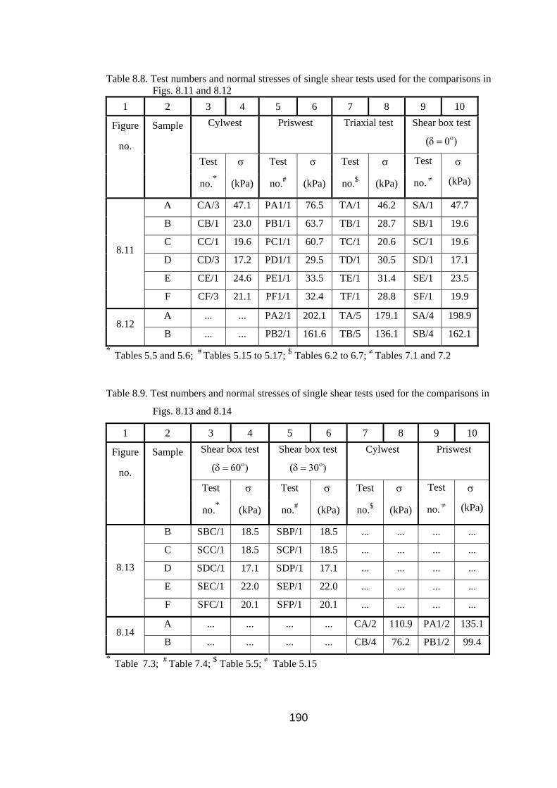
Table 8.8. Test numbers and normal stresses of single shear tests used for the comparisons in Figs. 8.11 and 8.12
1 2 3 4 5 6 7 8 9 10 Cylwest Priswest Triaxial test Shear box test
(δ = 0ο)
Test σ Test σ Test σ Test σ
Figure
no.
Sample
no.* (kPa) no.# (kPa) no.$ (kPa) no. ≠ (kPa)
A CA/3 47.1 PA1/1 76.5 TA/1 46.2 SA/1 47.7
B CB/1 23.0 PB1/1 63.7 TB/1 28.7 SB/1 19.6
C CC/1 19.6 PC1/1 60.7 TC/1 20.6 SC/1 19.6
D CD/3 17.2 PD1/1 29.5 TD/1 30.5 SD/1 17.1
E CE/1 24.6 PE1/1 33.5 TE/1 31.4 SE/1 23.5
8.11
F CF/3 21.1 PF1/1 32.4 TF/1 28.8 SF/1 19.9
A ... ... PA2/1 202.1 TA/5 179.1 SA/4 198.9 8.12
B ... ... PB2/1 161.6 TB/5 136.1 SB/4 162.1 * Tables 5.5 and 5.6; # Tables 5.15 to 5.17; $ Tables 6.2 to 6.7; ≠ Tables 7.1 and 7.2
Table 8.9. Test numbers and normal stresses of single shear tests used for the comparisons in
Figs. 8.13 and 8.14
1 2 3 4 5 6 7 8 9 10 Shear box test
(δ = 60ο)
Shear box test
(δ = 30ο)
Cylwest Priswest
Test σ Test σ Test σ Test σ
Figure
no.
Sample
no.* (kPa) no.# (kPa) no.$ (kPa) no. ≠ (kPa)
B SBC/1 18.5 SBP/1 18.5 ... ... ... ...
C SCC/1 18.5 SCP/1 18.5 ... ... ... ...
D SDC/1 17.1 SDP/1 17.1 ... ... ... ...
E SEC/1 22.0 SEP/1 22.0 ... ... ... ...
8.13
F SFC/1 20.1 SFP/1 20.1 ... ... ... ...
A ... ... ... ... CA/2 110.9 PA1/2 135.18.14
B ... ... ... ... CB/4 76.2 PB1/2 99.4 * Table 7.3; # Table 7.4; $ Table 5.5; ≠ Table 5.15
190

2. The bar charts in Fig. 8.11 show that cylwests (δ = 60o) yield higher values
of φd (by between 7.2o and 8.9o, average difference 7.9o) than shear box tests (δ = 0o).
A similar tendency is also observed in the results of test series under the lower
σ ranges (Table 8.7, column 14), and probably results from the higher values of δ in
the cylwests.
3. The bar charts in Fig. 8.11 show that priswests (δ = 30o) yield higher
values of φd than shear box tests (δ = 0o) for samples A to F at the lower density
under the lower σ range. Differences in the φd values are found as 2.0o, 1.5o, and 3.7o
for samples A to C; and as 4.1o, 3.4o, and 5.6o for samples D to F respectively. Lower
differences in the φd values for samples A to C are probably due to the distinctly
higher differences in the normal stresses in the corresponding priswests than in the
shear box tests with δ = 0o (Table 8.8, columns 6 and 10). The bar charts in Fig. 8.12
show that the φd value measured in priswests are higher than those in shear box tests
(δ = 0o) by 0.4o and 1.6o for samples A and B respectively. Higher φd values
measured in priswests than in shear box tests is also seen from the results of the test
series under the lower, higher, and combined σ ranges (Table 8.7, columns 15, 17,
and 19), and probably results from the higher values of δ in the priswests.
4. The bar charts in Figs. 8.11 show that triaxial tests (δ ≅ 65o) yield higher
values of φd (by between 3.0o and 6.1o, average difference 4.2o) than shear box tests
(δ = 0o) for samples A to F at the lower density under the lower σ range. The bar
charts in Fig. 8.12 show that the φd value measured in triaxial tests are higher than
those in shear box tests (δ = 0o) by 0.7o and 0.8o for samples A and B respectively.
Higher φd values measured in triaxial tests than in shear box tests is also seen from
the results of the test series under the lower, higher, and combined σ ranges (Table
8.7, columns 16, 18, and 20), and probably results from the higher values of δ in the
triaxial tests.
191
5. The bar charts in Fig. 8.13 show that shear box tests with δ = 60o yield
higher φd values (by between 2.1o and 7.4o, average difference 4.4o) than shear box
tests with δ = 30o for samples B to F under the lower σ range. A similar tendency is
observed in the results obtained from shear box test series with δ = 60o and δ = 30o
under the lower σ ranges (Table 8.7, column 22). The difference in the φd values
with change in δ is similar to that observed in cylwests (δ = 60o) and priswests
(δ = 30o) under the lower σ range (Fig. 8.14): cylwests yield higher φd values than
priswests by 1.9o and 2.1o for samples A and B respectively. These results, as well as
those in Table 8.7, columns 21 and 22, are verifications of the earlier argument that
cylwests yield higher φd values than priswests due to the larger δ in the cylwests
(section 8.1.1, paragraph (4)).
6. The value of the peak friction angle φd measured in single cylwests on
previously untested specimens for samples A and B were 57.1o and 53.3o respectively
(Fig. 8.11). When these sheared specimen were tested a second time (Fig. 8.14), the
φd values decreased to 52.6o and 47.8o, indicating differences of 4.5o and 5.5o. Such
results raised the question of whether the reason for cylwests yielding higher φd
values than shear box tests (δ = 60o) (Table 8.7, columns 2 and 12) could be the use
of specimens previously sheared more than once in the shear box tests. So an
additional cylwest (Table 8.10), at the lower density under the lower σ range, was
performed on each of the samples B to F using specimens prepared from the same
batch of the samples as those from which the shear box (δ = 60o) specimens had been
prepared. The normal stress σ in these tests (Table 8.10, column 4) were close to
those in the second tests of shear box test series SBC to SFC (Table 7.3); so the
results of these second tests were used for the bar chart comparisons in Fig. 8.15.
Fig. 8.15 shows that the φd values measured in cylwests and shear box tests are nearly
the same for samples C and E; cylwests yield lower φd values than shear box tests by
1.7o, 1.1o and 3.1o for samples B, D, and F respectively. It is seen that the average
difference between the cylwest and shear box test results has decreased from 5o
192
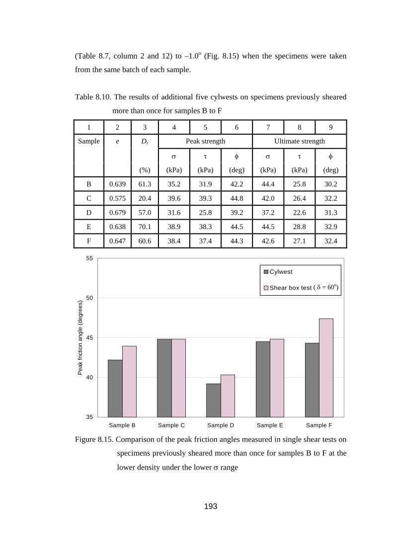
(Table 8.7, column 2 and 12) to –1.0o (Fig. 8.15) when the specimens were taken
from the same batch of each sample.
Table 8.10. The results of additional five cylwests on specimens previously sheared
more than once for samples B to F
1 2 3 4 5 6 7 8 9
Peak strength Ultimate strength Dr
σ τ φ σ τ φ
Sample e
(%) (kPa) (kPa) (deg) (kPa) (kPa) (deg)
B 0.639 61.3 35.2 31.9 42.2 44.4 25.8 30.2
C 0.575 20.4 39.6 39.3 44.8 42.0 26.4 32.2
D 0.679 57.0 31.6 25.8 39.2 37.2 22.6 31.3
E 0.638 70.1 38.9 38.3 44.5 44.5 28.8 32.9
F 0.647 60.6 38.4 37.4 44.3 42.6 27.1 32.4
35
40
45
50
55
Sample B Sample C Sample D Sample E Sample F
Pea
k fri
ctio
n an
gle
(deg
rees
)
Cylwest
Shear box test ( δ = 60
o)
Figure 8.15. Comparison of the peak friction angles measured in single shear tests on
specimens previously sheared more than once for samples B to F at the
lower density under the lower σ range
193

8.1.3 Possible Effect of Particle Crushing on Measured Relative
Density and Shear Strength The relative density Dr values given in Tables 5.5 to 5.7 for cylwest; 5.15 to
5.19 for priswests; 6.2 to 6.10 for triaxial tests; 7.1 to 7.4 for shear box test; and 8.10
for the additional cylwests were calculated on the basis of the dry density ρd of the
specimens, and the emax and emin values determined by using ρmax and ρmin as in
section 4.3. When a specimen, which has crushed to some extent in a previous shear
test (or tests), is re-tested, a lower compactive effort is sufficient to produce the ρd
value obtained for previously untested specimens because of the finer particles filling
the spaces between the coarser ones. Also the emax and emin values obtained for
previously untested specimens are not valid for previously sheared specimens. So the
true Dr values of previously sheared specimens are probably lower than given in the
tables listed above, and this may be part of the reason for the significant drop in φd
values in tests on such specimens on being re-sheared.
8.2 Comparison of the Results of the Shear Tests with Existing
Empirical Relationships
The relationships obtained from equation (2.13), given by Schanz & Vermeer
(1996), and equation (2.8), given by Wroth (1984), for samples A to F at the lower
density and for samples D to F at the higher density are shown in Figs. 8.16 and 8.17,
respectively. Equation (2.13) is represented as full lines, starting with the
corresponding φcv, taken as the average of the ultimate friction angles measured in
the wedge shear tests (Table 8.5, columns 2 and 5); equation (2.8) is represented by
dashed lines. The peak friction angles measured in wedge shear tests (assumed to be
plane strain tests) have been plotted in Figs. 8.16 and 8.17 against the corresponding
values measured in triaxial tests. To eliminate the effect of crushing in previous shear
tests, peak friction angles φcu, φpu, and φtu measured in single cylwest, priswest, and
triaxial tests respectively in which previously untested specimens had been used are
also compared in these figures.
194
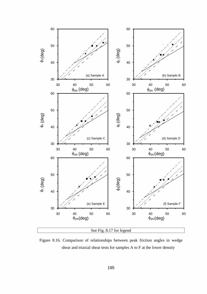
30 40 50 60
30 40 50 60 (deg)
30
40
50
60
(deg
)
30
30
30 40 50 60
30 40 50 60
30
40
50
60
(deg
)
φ
t
φ
t
(a) Sample A (b) Sample B
(deg)φps
40 50 60 (deg)
φps
30
40
50
60
(deg
)
40 50 (
φps
60deg)
30
40
50
60
(deg
)
φps
φ t
φt
(c) Sample C (d) Sample D
( φps deg)
30
40
50
60
(deg
)
( φps deg)
30
40
50
60
(deg
)
φ t
φ t
(e) Sample E (f) Sample F
See Fig. 8.17 for legend Figure 8.16. Comparison of relationships between peak friction angles in wedge
shear and triaxial shear tests for samples A to F at the lower density
195

30 40 50 60
30 40 50 60 (deg)
30
40
50
60
(deg
)
30 40 50 60 (deg)
30
40
50
60
(deg
)
30
40
50
60
(deg
)
φ t
φ t
(a) Sample D
(b) Sample E
(deg) φps φps
• φcu vs φtu; o φpu vs φtu; υ φc vs φtl
ν φpl vs φtl; σ φph vs φth; Υ φpa vs φta
45-degree line
Schanz & Vermeer’s (1996) eqn. (2.13)
Wroth’s (1984) eqn. (2.8)
........... Equation (8.1)
φt
(c) Sam
φps
ple F
Figure 8.17. Comparison of relationships between peak friction angles in wedge
shear and triaxial shear tests for samples D to F at the higher density
From Figs. 8.16 and 8.17, it can be seen that the plotted points representing
cylwest versus triaxial test results, especially on untested specimens, (except for
sample B at the lower density (Fig. 8.16(b)) and sample E at the higher density
(Fig. 8.17(b)), all lie above but are quite close to both of the representations of
equations (2.8) and (2.13). This tendency is in good agreement with Mirata and
Gökalp’s (1997) findings (section 2.1.4, paragraph (18)), and is a verification of the
earlier argument that the wedge shear test is similar although not identical with the
conventional plane strain test (section 2.4), when the orientation of the shear plane to
the bedding plane is about the same.
196
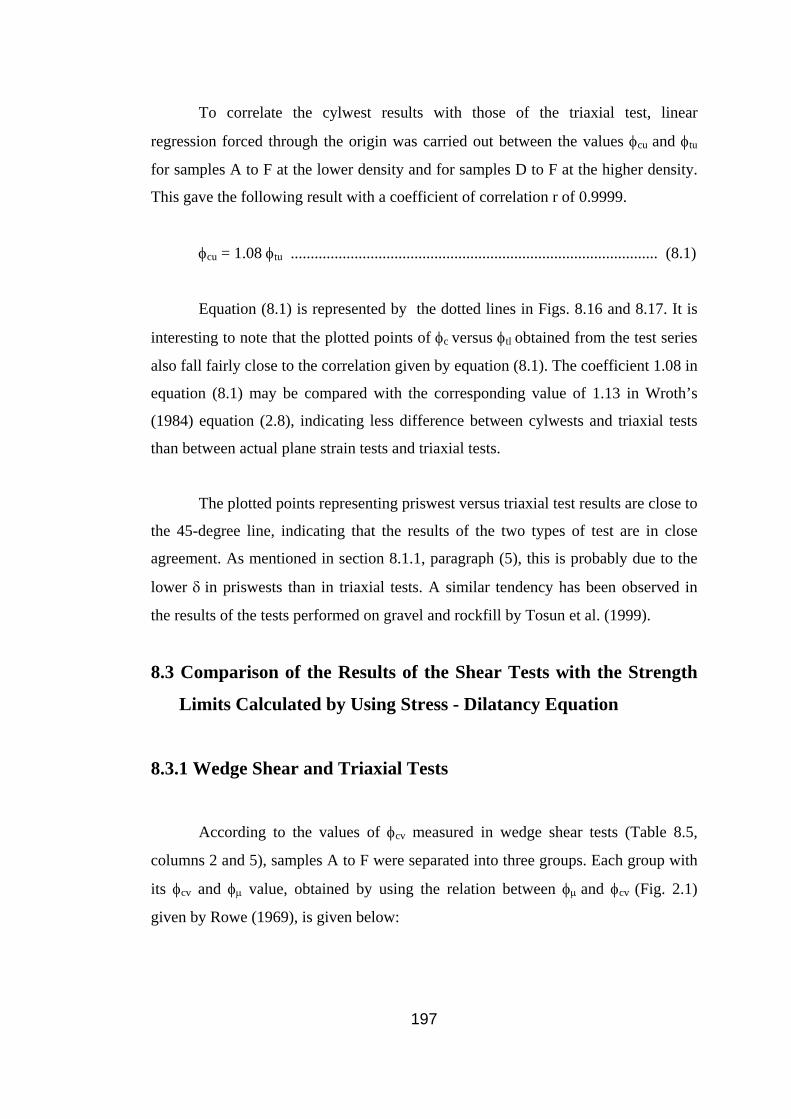
To correlate the cylwest results with those of the triaxial test, linear
regression forced through the origin was carried out between the values φcu and φtu
for samples A to F at the lower density and for samples D to F at the higher density.
This gave the following result with a coefficient of correlation r of 0.9999.
φcu = 1.08 φtu ............................................................................................ (8.1)
Equation (8.1) is represented by the dotted lines in Figs. 8.16 and 8.17. It is
interesting to note that the plotted points of φc versus φtl obtained from the test series
also fall fairly close to the correlation given by equation (8.1). The coefficient 1.08 in
equation (8.1) may be compared with the corresponding value of 1.13 in Wroth’s
(1984) equation (2.8), indicating less difference between cylwests and triaxial tests
than between actual plane strain tests and triaxial tests.
The plotted points representing priswest versus triaxial test results are close to
the 45-degree line, indicating that the results of the two types of test are in close
agreement. As mentioned in section 8.1.1, paragraph (5), this is probably due to the
lower δ in priswests than in triaxial tests. A similar tendency has been observed in
the results of the tests performed on gravel and rockfill by Tosun et al. (1999).
8.3 Comparison of the Results of the Shear Tests with the Strength
Limits Calculated by Using Stress - Dilatancy Equation
8.3.1 Wedge Shear and Triaxial Tests
According to the values of φcv measured in wedge shear tests (Table 8.5,
columns 2 and 5), samples A to F were separated into three groups. Each group with
its φcv and φµ value, obtained by using the relation between φµ and φcv (Fig. 2.1)
given by Rowe (1969), is given below:
197

(a) Group 1 (Sample A) (φcv = 39.4o; φµ = 33o)
(b) Group 2 (Samples B, C, E, and F) (φcv = 35.2o; φµ = 28o)
(c) Group 3 (Sample D) (φcv = 33.6o; φµ = 26o)
Following Rowe (1969) (section 2.1.1), it was assumed that D (equation
(2.2)) varies approximately between 1 and 2 as the material passes from the loosest
to the densest state in both triaxial tests and wedge shear tests (assumed to be plane
strain tests). By substituting these D values in equation (2.1) together with the
limiting values of φf (given in section 2.1.1), the limiting values of peak friction
angle φd were calculated from the corresponding values of R (defined in section
2.1.1, and explained in Appendix A) for each group, both for the plane strain and the
triaxial tests. The limiting values for the plane strain tests were connected by a full
line, and those for the triaxial tests were connected by a dashed line, as shown in
Figs. 8.18 to 8.22. The peak friction angle of each sample in each group measured in
wedge shear and tiaxial test series under the lower, higher, and combined σ ranges
was also plotted against the average initial relative density Dr in Figs. 8.18 to 8.20.
The symbols in the legends used in Figs. 8.18 to 8.20 have been defined in section
8.1.1, paragraph (1), where it was also explained that the cylwest, priswest, and
triaxial test results are affected by different degrees of previous particle crushing in
specimens used for some of the tests. To compare the results of tests performed on
identical specimens, peak friction angles measured in single shear tests on previously
untested specimens were plotted against Dr values in Figs. 8.21 and 8.22. The
symbols in the legends used in Figs. 8.21 and 8.22 have been defined in section 8.2.
198
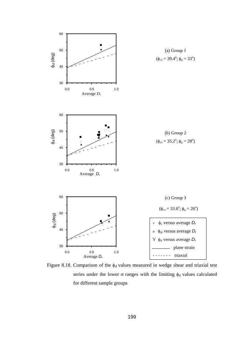
0.0 0.5 1.0 D
30
40
50
60
(de
g)
(a) Group 1
(φcv = 39.4o; φµ = 33o)
0.0 0.5 1.0
(b) Group 2
(φcv = 35.2o; φµ = 28o)
0.0 0.5 1.0
(c) Group 3
(φcv = 33.6o; φµ = 26o)
Average Dr D
30
40
50
60
(de
g)
Average Dr D
30
40
50
60
(de
g)
Average Dr
φ
d (d
eg)
φ
d (d
eg)
φ d (d
eg)
ν φc versus average Dr
σ φpl versus average Dr
Υ φtl versus average Dr
plane strain
- - - - - - - triaxial
Figure 8.18. Comparison of the φd values measured in wedge shear and triaxial test
series under the lower σ ranges with the limiting φd values calculated
for different sample groups
199

0.0 0.5 1.0 D
30
40
50
60
(de
g)
(a) Group 1
(φcv = 39.4o; φµ = 33o)
0.0 0.5 1.0
(b) Group 2
(φcv = 35.2o; φµ = 28o)
0.0 0.5 1.0D
30
40
50
(de
g)
(c) Group 3
(φcv = 33.6o; φµ = 26o)
φ d (d
eg)
Average Dr D
30
40
50
60
(de
g)
Average Dr
φ d (d
eg)
φ d
(deg
)
φ d
(deg
)
σ φph versus average Dr
Υ φth versus average Dr
plane strain - - - - - - - - triaxial
Average Dr
Figure 8.19. Comparison of the φd values measured in priswest and triaxial test series
under the higher σ ranges with the limiting φd values calculated for
different sample groups
200
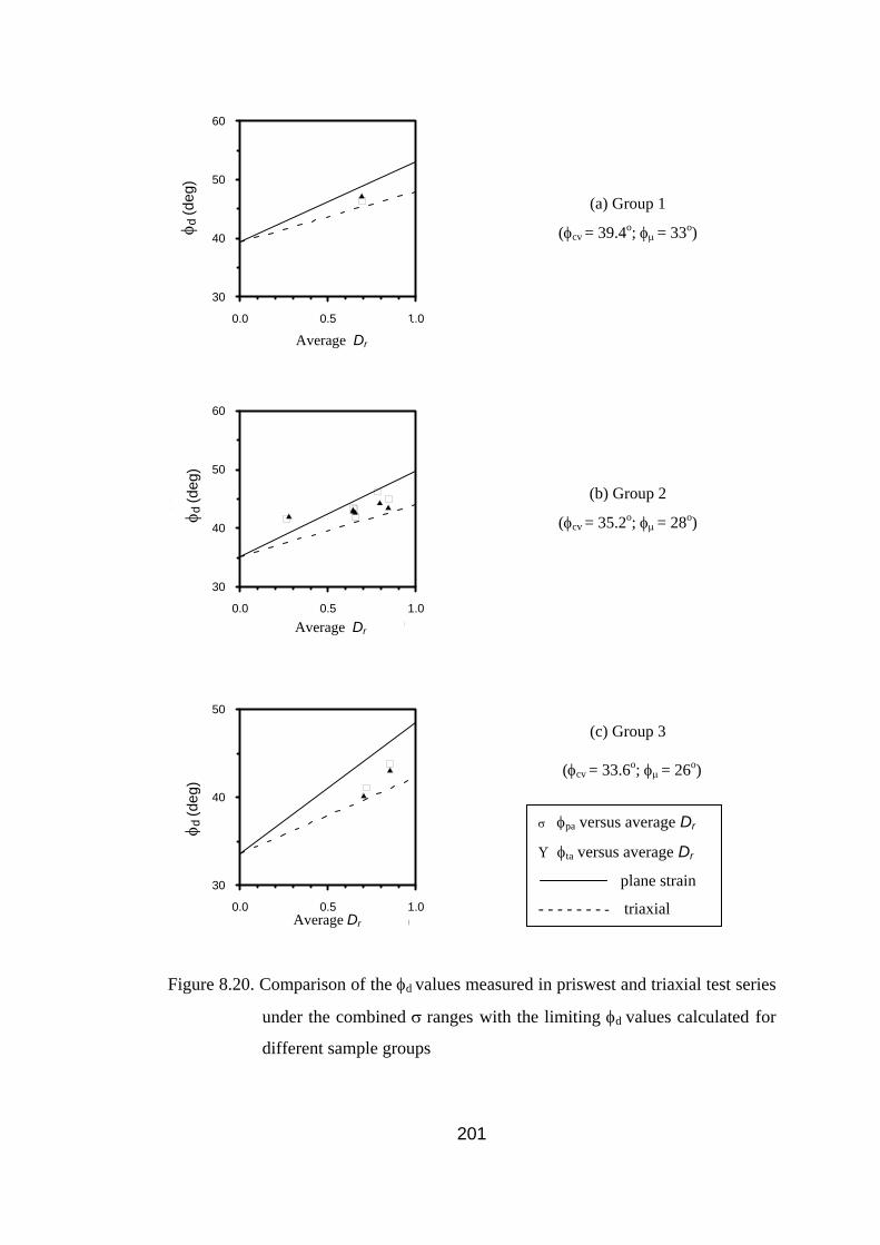
0.0 0.5 1.0 D
30
40
50
60
(de
g)
(a) Group 1
(φcv = 39.4o; φµ = 33o)
0.0 0.5 1.0
(b) Group 2
(φcv = 35.2o; φµ = 28o)
0.0 0.5 1.0
(c) Group 3
(φcv = 33.6o; φµ = 26o)
φ
d (d
eg)
Average Dr
Average Dr D
30
40
50
60
(de
g)
φ
d (d
eg)
Average Dr D
30
40
50
(de
g)
φd
(deg
)
σ φpa versus average Dr
Υ φta versus average Dr
plane strain
- - - - - - - - triaxial
Figure 8.20. Comparison of the φd values measured in priswest and triaxial test series
under the combined σ ranges with the limiting φd values calculated for
different sample groups
201

0.0 0.5 1.0 D
30
40
50
60
(de
g)
(a) Group 1
(φcv = 39.4o; φµ = 33o)
0.0 0.5 1.0
(b) Group 2
(φcv = 35.2o; φµ = 28o)
0.0 0.5 1.0
(c) Group 3
(φcv = 33.6o; φµ = 26o)
Dr D
30
40
50
60
(de
g)
Dr D
30
40
50
60
(de
g)
φd
(deg
)
φ d
(deg
)
φd
(deg
)
Dr
φ
d (d
eg)
ν φcu versus average Dr
σ φpu versus average Dr
Υ φtu versus average Dr
plane strain
- - - - - - - triaxial
Figure 8.21. Comparison of the φd values measured in single shear tests on previously
untested specimens under the lower σ range with the limiting φd values
calculated for different sample groups
202

0.0 0.5 1.0 D
30
40
50
60
(de
g)
(a) Group 1
(φcv = 39.4o; φµ = 33o)
0.0 0.5 1.0 D
30
40
50
60
(de
g)
(b) Group 2
(φcv = 35.2o; φµ = 28o)
0.0 0.5 1.0D
30
40
50
60
(de
g)
(c) Group 3
(φcv = 33.6o; φµ = 26o)
Dr
Dr
φ d
(deg
)
φd
(deg
)
φ d
(deg
)
Dr
σ φpu versus average Dr
Υ φtu versus average Dr
plane strain
- - - - - - - triaxial
Figure 8.22. Comparison of the φd values measured in single shear tests on previously
untested specimens under the higher σ range with the limiting φd values
calculated for different sample groups
203
For the cylwests, Fig. 8.21 shows that the plotted points representing φcu
versus Dr for each group are located well above the full line for the plane strain test.
A similar tendency is also observed in the plotted points representing φc versus
average Dr in cylwest series (Fig. 8.18), except those for group 3 in Fig. 8.18(c).
These results show that cylwests generally yield higher values of φd than those
calculated by using stress - dilatancy equation.
For the triaxial tests, Fig. 8.21 also shows that under the lower σ range, the
plotted points representing φtu versus Dr for each group are well above the dashed
line for the triaxial test. A similar tendency is also observed in the plotted points
representing φtl versus average Dr in triaxial test series under the lower σ range
(Fig. 8.18). Fig. 8.22 shows that the plotted point representing φtu versus Dr for group
1 is close to the dashed line for the triaxial test; that for group 2 is located well above
this line. In triaxial test series under the higher σ ranges (Fig. 8.19), three of the φth
values are located well above the dashed line for the triaxial test; the remaining six
φth values are close to this line. A similar tendency is observed in triaxial test series
under the combined σ ranges (Fig. 8.20).
For the priswests, Fig. 8.21 shows that under the lower σ range, the plotted
points representing φpu versus Dr for groups 1 and 3 are close to the full line for the
plane strain test; those for group 2 are located well above this line. Under the higher
σ range (Fig. 8.22), two of the φpu values are located below the line for the plane
strain test; in the remaining three, the φpu value is close to this line. In priswest series
under the lower σ ranges (Fig. 8.18), the plotted points representing φpl versus
average Dr for each group are close to the full line for the plane strain test. In
priswest series under the higher σ ranges (Fig. 8.19), three of the φph values are
located well below the full line for the plane strain test; the remaining six φph values
are close to this line. A similar tendency is observed in priswest series under the
combined σ ranges (Fig. 8.20).
204
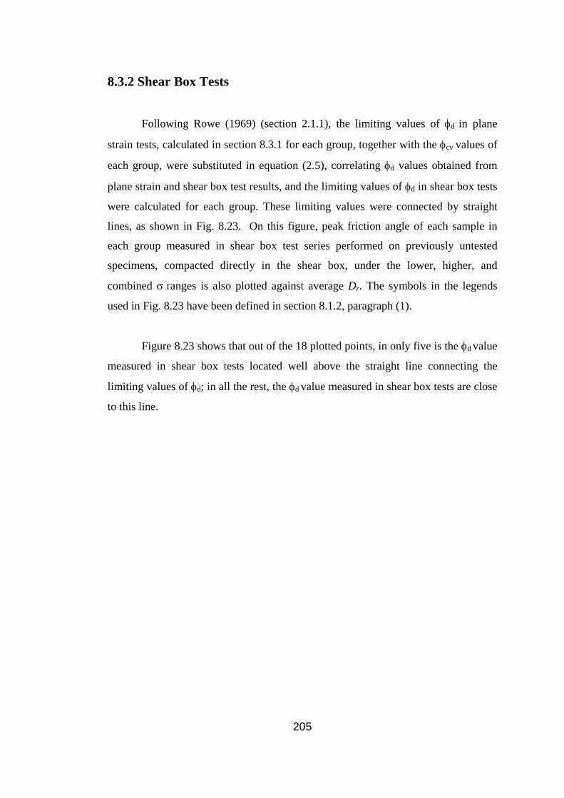
8.3.2 Shear Box Tests
Following Rowe (1969) (section 2.1.1), the limiting values of φd in plane
strain tests, calculated in section 8.3.1 for each group, together with the φcv values of
each group, were substituted in equation (2.5), correlating φd values obtained from
plane strain and shear box test results, and the limiting values of φd in shear box tests
were calculated for each group. These limiting values were connected by straight
lines, as shown in Fig. 8.23. On this figure, peak friction angle of each sample in
each group measured in shear box test series performed on previously untested
specimens, compacted directly in the shear box, under the lower, higher, and
combined σ ranges is also plotted against average Dr. The symbols in the legends
used in Fig. 8.23 have been defined in section 8.1.2, paragraph (1).
Figure 8.23 shows that out of the 18 plotted points, in only five is the φd value
measured in shear box tests located well above the straight line connecting the
limiting values of φd; in all the rest, the φd value measured in shear box tests are close
to this line.
205
0.0 0.5 1.0 D
30
35
40
45
50
(deg
)
(a) Group 1
(φcv = 39.4o; φµ = 33o)
0.0 0.5 1.0 D
25
30
35
40
45
(deg
)
(b) Group 2
(φcv = 35.2o; φµ = 28o)
0.0 0.5 1.0
(c) Group 3
(φcv = 33.6o; φµ = 26o)
Average Dr D
25
30
35
40
45
deg)
(
φd
(deg
)
Average Dr
Average Dr
φ d
(deg
)
φd
(deg
)
ν φsl versus average Dr
υ φsh versus average Dr
Υ φsh versus average Dr
Figure 8.23. Comparison of the φd values measured in shear box tests with the
limiting φd values calculated for different sample groups
206
CHAPTER 9
CONCLUSIONS AND RECOMMENDATIONS
Particle crushing has occurred in all shear tests even under low normal
stresses. In the samples tested, it was verified that particle shape was not the only
factor influencing the crushing of particles; other important factors were the strength
of the particles, and the gradation.
Cylwests yielded higher shear strength than priswests under the lower normal
stress σ range (between 17 kPa and 59 kPa). This is probably due to the difference in
the inclination δ of the shear plane to the bedding planes: δ is 60o in cylwests, while
in priswests using the 30o mould δ is 30o.
Cylwests yielded higher shear strength than triaxial tests under the lower σ
range, and there was some indication that this difference in strength was linked with
the φcv values of the samples, as observed by past researchers. The results of the
cylwests and triaxial tests, especially on untested specimens, were quite close to the
existing correlations between φps obtained from actual plane strain tests and φt from
triaxial tests. This indicated that the wedge shear test is similar although not identical
with the conventional plane strain test, when the orientation of the shear plane to the
bedding planes is about the same. Correlating the results on previously untested
specimens, the φcu from cylwests were found to be 1.08 times the φtu from triaxial
tests; the corresponding ratio between actual plane strain test and triaxial test results
given by Wroth’s (1994) equation (2.8) is 1.13.
207
The results of priswests and triaxial tests under the same σ ranges are in close
agreement; this is probably due to the lower δ in priswests than in triaxial tests. This
may also explain the close agreement between priswests and triaxial tests on < 40
mm gravel and crushed rock reported by Tosun et al. (1999).
Shear box tests (δ = 0o) performed on specimens compacted directly in the
shear box yielded lower shear strength than both wedge shear and triaxial shear tests
under the same σ ranges. It was shown that the shear strength measured in shear box
showed an increase when δ was increased from 30o to 60o; this increase was of the
order of the difference between priswest (δ = 30o) and cylwest (δ = 60o) results
mentioned earlier. Shear box specimens with δ = 60o, prepared from the same batch
of any sample as the corresponding cylwests, yielded nearly the same strength as that
obtained in cylwests (δ = 60o).
When the triaxial shear tests could be sufficiently prolonged to yield the
ultimate strength, the φcv values measured in the wedge shear test and the triaxial test
were nearly the same.
Following Rowe (1969), the results of the wedge shear, triaxial, and shear
box tests were compared with the strength limits calculated by using the stress –
dilatancy equation for plane strain, triaxial, and shear box tests. Compared to the
calculated values, under the lower σ ranges, cylwests generally yielded higher shear
strength; under the lower σ ranges, priswests generally yielded nearly the same shear
strength, triaxial tests yielded higher shear strength; under the higher and combined
σ ranges, priswests yielded lower shear strength, triaxial tests yielded nearly the
same shear strength. The shear strength measured in shear box tests was generally
close to the calculated values.
208

As an overall conclusion, it can be said that for the analysis of a plane strain
type of problem like the stability of slopes in sand, the cylwest or the priswest may
be used depending on in which test the inclination of the shear plane to the bedding
planes is closer to the average inclination in the actual stability problem. If the size of
the particles permit, the shear box test may be used, provided specimens are prepared
with the correct inclination of the shear plane to the bedding planes. Triaxial tests
would give a conservative factor of safety, and conventional shear box tests with
horizontal bedding planes even more conservative values for such problems.
For future studies, the following recommendations can be made.
(a) Each shear test should be performed on an untested specimen to eliminate
the effect of particle crushing.
(b) To determine the effect on shear strength of mineral composition, more
detailed mineralogical analyses should be carried out, including the determination of
individual percentages of each ingredient.
(c) The effect of δ on the peak friction angle measured in priswests may be
investigated by modifying the test mould (Fig. 5.9(b)) so that the side of the mould
on which the main load is applied becomes the removable lid.
(d) Slope failures in sand may be studied and back analyses performed to
estimate the φd mobilized in the slips and compare these with the laboratory test
results.
209
REFERENCES
Adel, H. (2001). Determination of Plane Strain Shear Strength of Sand from the
Results of Triaxial Tests. Canadian Geotechnical Journal 38, pp. 1231-
1240.
Aybak, T. (1988). Improved Measurement of Shear Strength in the In Situ Wedge
Shear Test. MS thesis, Middle East Technical University, Ankara.
Barden, L. & Khayatt, A.J. (1966). Incremental Strain Rate Ratios and Strength of
sand in the Triaxial Test . Géotechnique 16, No. 4, pp. 338 – 357.
Bardet, J. P. (1997). Experimental Soil Mechanics. Prentice Hall, New Jersey.
Bishop, A.W. (1966). The Strength and Soils as Engineering Materials.
Géotechnique 16, No. 2, pp. 91 – 130.
Bolton, M.D. (1986). The Strength and Dilatancy of Sands. Géotechnique
36, No. 1, pp. 65 – 78.
Cornforth, D.K. (1964). Some Experiments on the Influence of Strain Conditions on
the Strength of Sand. Géotechnique 14, No. 2, pp. 143 – 167.
Cornforth, D.K. (1973). Prediction of Drained Strength of Sands from Relative
Density Measurements. ASTM Special Technical Publication 523, pp. 281 –
303.
210
Çağnan, Ş. (1990). Measurement of Shear Strength of Coarse Gravels by the Wedge
Shear Test. MS thesis, Middle East Technical University, Ankara.
Dobkins & Folk. (1970). Shape Development on Tahiti – Nui. Journal of
Sedimentary Petrology 40, pp. 1167 – 1203.
Girgin, İ. (2000). Results of Mineralogical Analyses. Unpublished work. Mineral
Research and Exploration Directorate Laboratories, Ankara.
Gökalp, A. (1994). Investigation of Certain Problems related with the Wedge Shear
Test. MS thesis, Middle East Technical University, Ankara.
Gün, F. (1997). Comparison of the Shear Strength of Statically and Dynamically
Compacted Clays. MS thesis, Middle East Technical University, Ankara.
Gürol, A. (2000). Effect of Curing on the Undrained Shear Strength of Compacted
Clays. MS thesis, Middle East Technical University, Ankara.
Hardin, B.O. (1985). Crushing of Soil Particles. Getechnical Testing Journal 14, No.
3, pp. 296 – 308.
Holubec, I. & D’Appolonia, E. (1973). Effect of Particle Shape on the Engineering
Properties of Granular Soils. ASTM Special Technical Publication 523, pp.
304 – 318.
Hussaini, M.M. (1973). Influence of Relative Density and Deformation of
Sand under Plane Strain Conditions. ASTM Special Technical
Publication 523, pp. 332 – 347.
Jewell, R. A. (1989). Direct Shear Tests on Sand. Géotechnique 39, No.2, pp. 309 –
322.
211
Kezdi, A. (1974). Handbookof Soil Mechanics. Elsevier Scientific Publishing
Company, New York.
Kirkpatrick, W.M. (1965). Effects of Grain Size and Grading on the Shear
Behaviour of Granular Materials. Proceedings of 6th International
Conference on Soil Mechanics and Foundation Engineering, Montreal 1, pp.
273 –277.
Koerner, M.R. (1970). Effect of Particle Characteristics on Soil Strength.
Journal of Soil Mechanics and Foundation Division, ASCE 96, SM4, pp.
1221 –1234.
Lambe, W.T. & Whitman, R.V. (1979). Soil Mechanics. John Wiley, USA.
Lee, K.L. (1970). Comparison of Plane Strain and Triaxial Tests on Sand.
Journal of Soil Mechanics and Foundation Division, ASCE 96, SM3, pp.
901 –923.
Leussink, H. & Wittke, W. (1963). Difference in Triaxial and Plane Strain
Shear Strength. ASTM Special Technical Publication. No.361, pp. 281 –
303.
Maeda, K. & Miura, K. (1999(a)). Relative Density Dependency of Mechanical
Properties of Sands. Soils and Foundations 39, No. 1, pp. 69 - 79.
Maeda, K. & Miura, K. (1999(b)). Confining Stress Dependency of Mechanical
Properties of Sands. Soils and Foundations 39, No. 1, pp. 53 - 67.
Marachi, N.D., Duncan, J.M., Chan, C.K., & Seed, H.B. (1981). Plane Strain Testing
of Sand . ASTM Special Technical Publication. No. 740, pp. 294 -302
212
Marsal, R.J. (1967). Large Scale Testing of Rockfill Materials. Journal of Soil
Mechanics and Foundation Division, ASCE 93, SM2, pp. 27 –43.
Mirata, T. (1974). The In Situ Wedge Shear Test -- A New Technique in Soil
Testing. Géotechnique 24, No.3, pp. 311–332. Corrigenda: Géotechnique
24, No.4, p. 698; 25, No.1, pp. 157-158; 36, No.1, p. 144; 37, No.3, p. 420;
38, No.1, p. 163.
Mirata, T. (1976). Short-term Stability of Slopes in Ankara Clay. PhD Thesis,
University of London.
Mirata, T. (1991). Developments in Wedge Shear Testing of Unsaturated Clays and
Gravels. Géotechnique 41, No.1, pp. 79 – 100. Corrigenda: Géotechnique
41, No.2, p. 296 and 41, No.4, pp. 639.
Mirata, T. (1992). Author’s Reply to Discussion on Developments in Wedge Shear
Testing of Unsaturated Clays and Gravels. Géotechnique 42, No.4, pp. 645-
648.
Mirata, T. (2000). Test Procedure for the Triaxial Shear Test on Sand. Unpublished
Work. Middle East Technical University, Ankara.
Mirata, T. (2001). Test Procedure for the Shear Box Test on Sand. Unpublished
Work. Middle East Technical University, Ankara.
Mirata, T. (2002(a)). TRIAX02. A Computer Program for the Evaluation of Triaxial
Tests. Middle East Technical University, Ankara.
Mirata, T. (2002(b)). DIST02. A Computer Program for the Evaluation of Shear Box
Tests. Middle East Technical University, Ankara.
213
Mirata, T. (2002(c)). Examination of the Effect on Cylwest Results of the Use of the
Double-cut Cylwest Mould with no Trimming. Unpublished Work. Middle
East Technical University, Ankara.
Mirata, T. (2003(a)). Manual for Wedge Shear Testing of Soils. Department of Civil
Engineering, Middle East Technical University, Ankara. (obtainable from
ULAKBİM Library)
Mirata, T. (2003(b)). Comparison of the Wedge Shear Test with the Plane Strain
Test. Unpublished Work. Middle East Technical University, Ankara.
Mirata, T. & Gökalp, A. (1997). Discussion. Géotechnique 47, No.4, pp. 887 – 889.
Mitchell, J.K. (1976). Fundamentals of Soil Behaviour. Wiley & Sons. USA
Norman, T. (2000(a)). Personal Communication. Middle East Technical University,
Ankara.
Norman, T. (2000(b)). Personal Communication. Middle East Technical University,
Ankara.
Norman, T. (2000(c)). Sedimentary Petrography Class Notes. Unpublished Work.
Middle East Technical University, Ankara.
Oda, M., Koishikawa, I., & Higuchi, T. (1978). Experimental Study of Anisotropic
Shear Strength of Sand by Plane Strain Test. Soils and Foundations 18, No.
1, pp. 25–37.
Riley, N.A. (1941) Projection Sphericity. Journal of Sedimentary Petrology 1, pp. 94
– 97.
214
Rowe, P. W. (1962). The Stress- Dilatancy Relation for Static Equilibrium of an
Assembly of Particles in Contact. Proc. R. Soc. A 269, pp. 500- 527.
Rowe, P. W. (1969). The Relation between the Shear Strength of Sands in Triaxial
Compression, Plane Strain, and Direct Shear. Géotechnique 19, No. 1,
pp. 75 – 86.
Şakar, M. (1997). Wedge Shear Testing of Clayey Gravels under Higher Normal
Stresses. MS thesis, Middle East Technical University, Ankara.
Schanz, T. & Vermeer, P.A. (1996). Angles of Friction and Dilatancy of Sand.
Géotechnique 46, No. 1, pp. 145 – 151.
Seed, H.B. & Lee, K.L. (1967). Drained Strength Characteristics of Sand. Journal of
Soil Mechanics and Foundation Division, ASCE 93, SM6, pp. 117 –141.
Shahu, J. T., & Yudhbir (1998). Model Tests on Sands with Different Angularity and
Mineralogy. Soils and Foundations 38, No. 4, pp. 151 –158.
Tatsuoka, F., Sakamato, M., Kawamura, T., & Fukushima, S. (1986). Strength and
Deformation Characteristics of Sand in Plane Strain Compression at
Extremely Low Pressures. Soils and Foundations 26, No. 1, pp. 65 –84.
Timeshenko, S. & Goodier, J.N. (1970). Theory of Elasticity, McGraw Hill, New
York
Tosun, H., Mirata, T., Mollamahmutoğlu, M., & Çolakoğlu, N.S. (1999). Shear
Strength of Gravel and Rockfill Measured in Triaxial and Plane Strain
Tests. Electronic Journal of Geotechnical Engineering:
http://www.ejge.com/
215
Ueng, T. & Chen, T. (2000). Energy Aspects of Particle Breakage in Drained Shear
of Sands. Géotechnique 50, No. 1, pp. 65– 72.
Vesic, A.S. & Clough, G.W. (1968). Behavior of Granular Materials under High
Stresses. Journal of Soil Mechanics and Foundation Division, ASCE 94,
SM3, pp. 661–687.
Wroth, C.P. (1984). The Interpretation of In Situ Soil Tests. Géotechnique 34, No. 4,
pp. 449 – 489.
Youd, T.L. (1973). Factors Controlling Maximum and Minimum Densities of Sands.
ASTM Special Technical Publication 523, pp. 98 – 112.
Yudhbir & Rahim, A. (1991). Quantification of Particle Shape and Angularity Using
the Image Analyzer. Getechnical Testing Journal 14, No. 3, pp. 296 – 308.
__________ (1987). İnşaat Mühendisliği için Zemin Deneyleri, TS 1900 Türk
Standardları Enstitüsü, Ankara.
__________ (1990). Soils for Civil Engineering Purposes; part 4, Compaction-
related Tests. BS 1377 British Standards Institution.
216

APPENDIX A
CALCULATION OF PEAK FRICTION ANGLE φd FROM THE
VALUES OF R
From Fig. A.1, sinφd is
⎟⎠⎞
⎜⎝⎛ σ+σ
⎟⎠⎞
⎜⎝⎛ σ−σ
=φ
2
2sin31
31
d = ⎟⎟⎠
⎞⎜⎜⎝
⎛σ+σσ−σ
31
31 =
⎟⎟⎠
⎞⎜⎜⎝
⎛+
σσ
⎟⎟⎠
⎞⎜⎜⎝
⎛−
σσ
=
⎟⎟⎠
⎞⎜⎜⎝
⎛+
σσ
σ
⎟⎟⎠
⎞⎜⎜⎝
⎛−
σσ
σ
1
1
1
1
3
1
3
1
3
13
3
13
................................. (A.1)
By replacing 3
1σσ
by R, the φd value is obtained as
⎟⎠⎞
⎜⎝⎛
+−
=φ −1R1Rsin 1
d ................................................................................................(A.2)
217217
φd
Failure envelope τ
σ
Figure A.1. Sketch showing the state of stress for sands
σ3 σ1
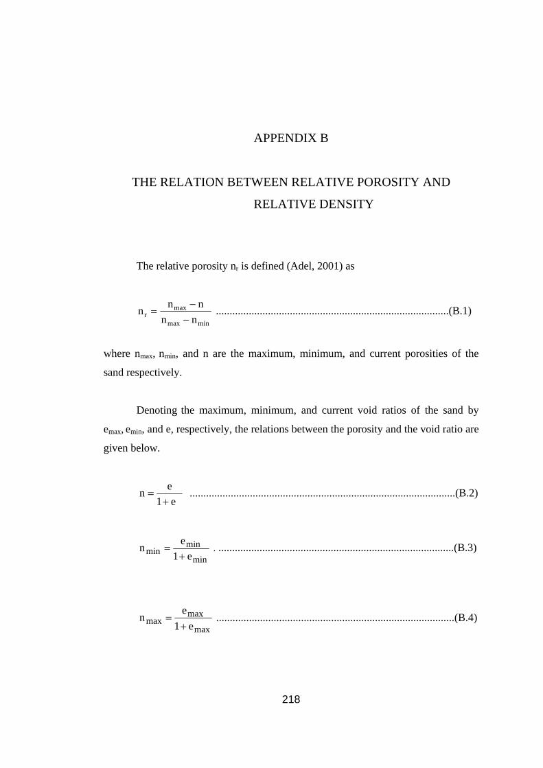
APPENDIX B
THE RELATION BETWEEN RELATIVE POROSITY AND
RELATIVE DENSITY
The relative porosity nr is defined (Adel, 2001) as
minmax
maxr nn
nnn−
−= .....................................................................................(B.1)
where nmax, nmin, and n are the maximum, minimum, and current porosities of the
sand respectively.
Denoting the maximum, minimum, and current void ratios of the sand by
emax, emin, and e, respectively, the relations between the porosity and the void ratio are
given below.
e1
en+
= .................................................................................................(B.2)
min
minmin e1
en+
= . ......................................................................................(B.3)
max
maxmax e1
en+
= .......................................................................................(B.4)
218
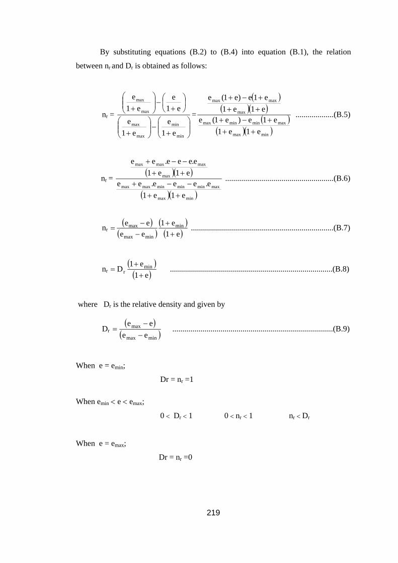
By substituting equations (B.2) to (B.4) into equation (B.1), the relation
between nr and Dr is obtained as follows:
nr =
⎟⎟⎠
⎞⎜⎜⎝
⎛+
−⎟⎟⎠
⎞⎜⎜⎝
⎛+
⎟⎠⎞
⎜⎝⎛
+−⎟⎟
⎠
⎞⎜⎜⎝
⎛+
min
min
max
max
max
max
e1e
e1e
e1e
e1e
=
( )( )( )
(( )( )
)minmax
maxminminmax
max
maxmax
e1e1e1e)e1(e
e1e1e1e)e1(e
+++−+
+++−+
...................(B.5)
nr = ( )( )
( )( )minmax
maxminminminmaxmax
max
maxmaxmax
e1e1e.eee.ee
e1e1e.eee.ee
++−−+
++−−+
......................................................(B.6)
nr ( )
( )( )
( )e1e1
eeee min
minmax
max
++
−−
= .......................................................................(B.7)
nr ( )
( )e1e1D min
r ++
= .................................................................................(B.8)
where Dr is the relative density and given by
Dr ( )
( )minmax
max
eeee
−−
= ................................................................................(B.9)
When e = emin;
Dr = nr =1 When emin < e < emax;
0 < Dr < 1 0 < nr < 1 nr < Dr
When e = emax;
Dr = nr =0
219
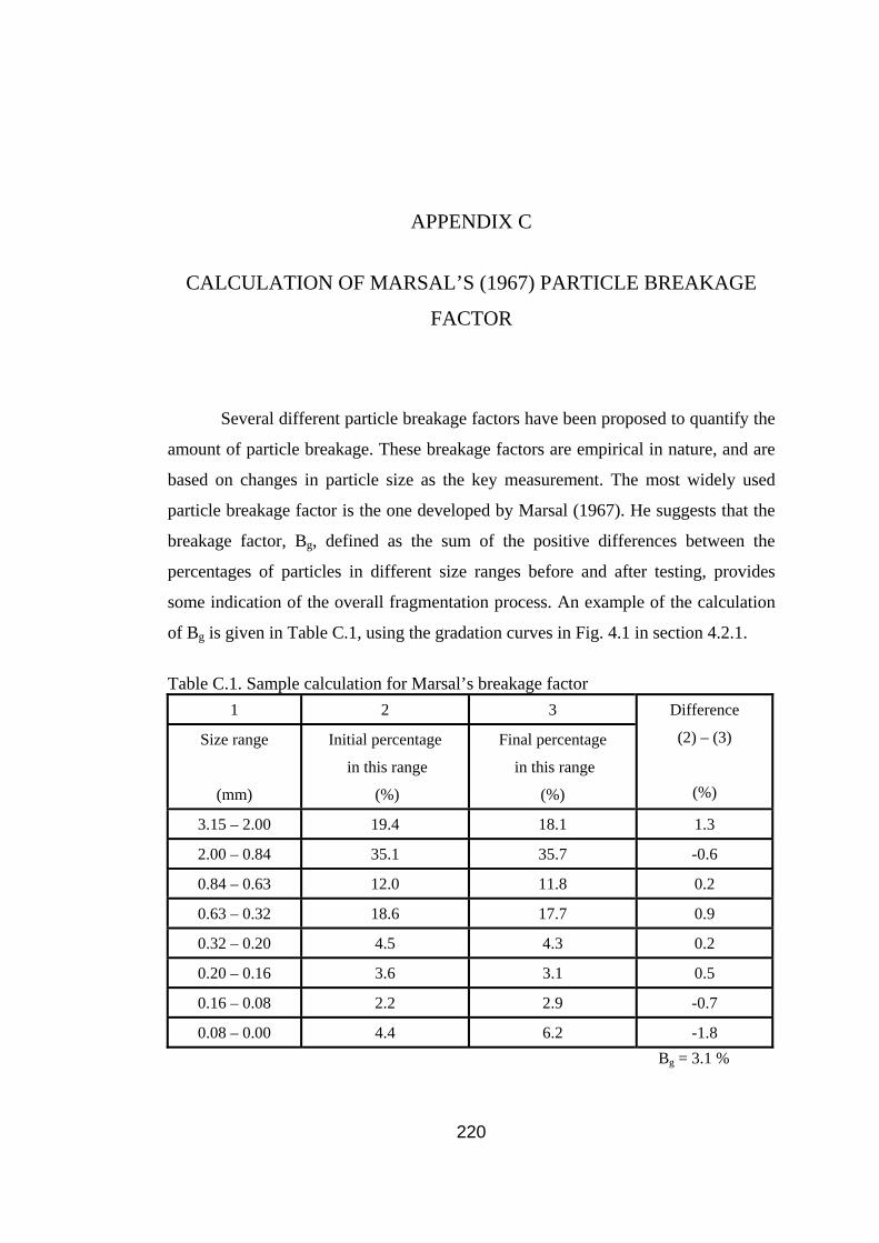
APPENDIX C
CALCULATION OF MARSAL’S (1967) PARTICLE BREAKAGE
FACTOR
Several different particle breakage factors have been proposed to quantify the
amount of particle breakage. These breakage factors are empirical in nature, and are
based on changes in particle size as the key measurement. The most widely used
particle breakage factor is the one developed by Marsal (1967). He suggests that the
breakage factor, Bg, defined as the sum of the positive differences between the
percentages of particles in different size ranges before and after testing, provides
some indication of the overall fragmentation process. An example of the calculation
of Bg is given in Table C.1, using the gradation curves in Fig. 4.1 in section 4.2.1.
Table C.1. Sample calculation for Marsal’s breakage factor
1 2 3
Size range
(mm)
Initial percentage
in this range
(%)
Final percentage
in this range
(%)
Difference
(2) – (3)
(%)
3.15 – 2.00 19.4 18.1 1.3
2.00 – 0.84 35.1 35.7 -0.6
0.84 – 0.63 12.0 11.8 0.2
0.63 – 0.32 18.6 17.7 0.9
0.32 – 0.20 4.5 4.3 0.2
0.20 – 0.16 3.6 3.1 0.5
0.16 – 0.08 2.2 2.9 -0.7
0.08 – 0.00 4.4 6.2 -1.8 Bg = 3.1 %
220
APPENDIX D
EXAMINATION OF THE EFFECT ON CYLWEST RESULTS
OF THE USE OF THE DOUBLE-CUT CYLWEST MOULD
WITH NO TRIMMING
According to the original design by Mirata (1991), the upper part of the shear
plane of TM (S) and the lower part of the shear plane of mobile part of the mould
TM (Fig. 5.3) should be chamfered slightly (see detail A in Fig. 5.2) to prevent the
soil in the opposite half from bearing on the test mould wall during shear. The test
mould used in the present study had no such chamfer. To examine the effect of this
defect on the test results, the shear plane was observed closely in a special cylwest on
sample E compacted at the lower density. It was seen that the part of the sand sample
moving past TM(S), being unrestrained in any way, did not bear on TM(S); there
was a distinct gap between this part of the sample and TM(S) as seen in Fig. D.1.
Apart from this observation, Mirata (2002(c)) repeated calculations for cylwest series
CA to CD (Tables 5.2 and 5.3), without applying an area correction, and it was seen
that the φ values both at peak and ultimate strength were not affected by more than
± 0.01o. So even if the separation shown in Fig. D.1 did not occur, and the tests were
evaluated without applying an area correction, the results would not significantly
differ from those presented in this thesis.
221
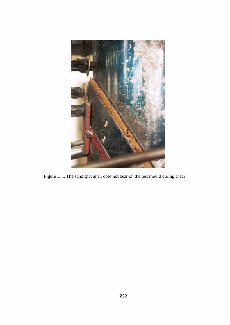
Figure D.1. The sand specimen does not bear on the test mould during shear
222
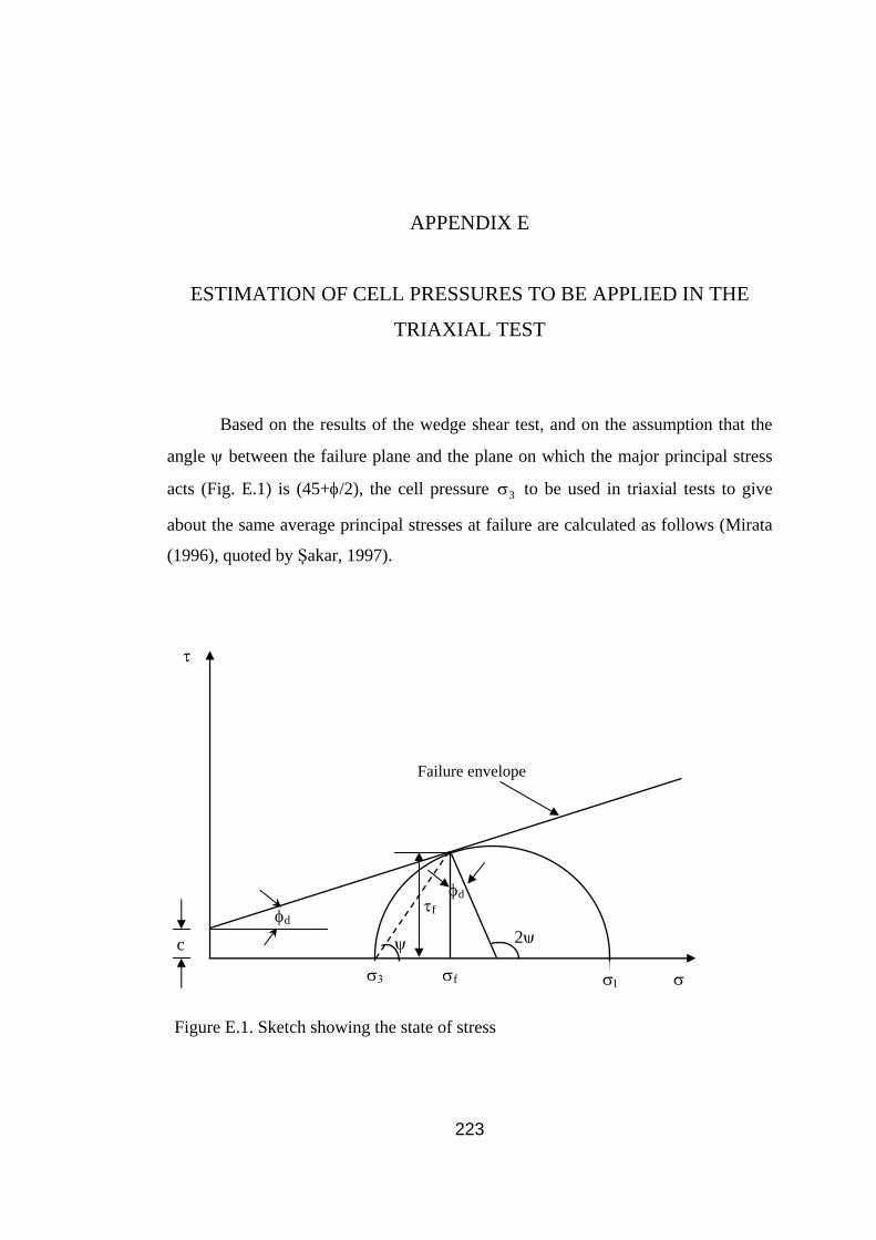
APPENDIX E
ESTIMATION OF CELL PRESSURES TO BE APPLIED IN THE
TRIAXIAL TEST
Based on the results of the wedge shear test, and on the assumption that the
angle ψ between the failure plane and the plane on which the major principal stress
acts (Fig. E.1) is (45+φ/2), the cell pressure 3σ to be used in triaxial tests to give
about the same average principal stresses at failure are calculated as follows (Mirata
(1996), quoted by Şakar, 1997).
Failure envelope
φd
σf σ3 σ1
Figure E.1. Sketch showing the state of stress
2ψ
τf φd
ψ
τ
c
σ
223

From Fig. E.1,
+σ=σ+σ
f31
2 τf tanφd.............................................................................(E.1)
For the same φd value, in the triaxial state of stress,
dd
d3131 sinsincos
c22
φ⎟⎟⎠
⎞⎜⎜⎝
⎛φφ
+σ+σ
=σ−σ
.......................................................(E.2)
For sands, c = 0. Then,
⎟⎠⎞
⎜⎝⎛ σ+σ
=σ−σ
223131 sinφd ................................................................... (E.3)
Also,
⎟⎠⎞
⎜⎝⎛ σ−σ
−⎟⎠⎞
⎜⎝⎛ σ+σ
=σ22
31313 .....................................................................(E.4)
Substituting equation (E.3) in equation (E.4),
⎟⎠⎞
⎜⎝⎛ σ+σ
=σ2
313 (1-sinφd)............................................................................(E.5)
Assuming plane strain conditions in the wedge shear test, the intermediate principal
stress is given by (e.g. Timeshenko & Goodier, 1970) 2σ
( )312 σ+σν=σ ........................................................................................(E.6)
where ν= poisson’s ratio.
224

The average principal stress σp is
⎟⎠⎞
⎜⎝⎛ σ+σ+σ
=σ3
321p .................................................................................(E.7)
Substituting equation (E.6) in equation (E.7)
( 31p 31
σ+σ⎟⎠⎞
⎜⎝⎛ ν+
=σ ) ................................................................................(E.8)
If ν = 0.3 is assumed (based on ν determinations on 5 mm – 10 mm gravel and on
unsaturated Ankara clay),
⎟⎠⎞
⎜⎝⎛ σ+σ
=σ23
6.2 31p ..................................................................................(E.9)
where ⎟⎠⎞
⎜⎝⎛ σ+σ
231 is estimated from equation (E.1)
After calculating σp for the wedge shear test in this way, one can equate this
to ⎟⎠⎞
⎜⎝⎛ σ+σ
231 in the triaxial test, and evaluate σ3 from equation (E.5) as
−σ=σ 1(p3 sinφd).....................................................................................(E.10)
An example of the calculation of σ3 values is given in Table E.1, using the φd
value of 39.7o obtained from the results of priswest series PD2 (Table 5.16).
225
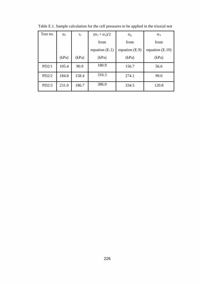
Table E.1. Sample calculation for the cell pressures to be applied in the triaxial test
Test no. σf
(kPa)
τf
(kPa)
(σ1 + σ3)/2
from
equation (E.1)
(kPa)
σp
from
equation (E.9)
(kPa)
σ3
from
equation (E.10)
(kPa)
PD2/1 105.4 90.9 180.9 156.7 56.6
PD2/2 184.8 158.4 316.3 274.1 99.0
PD2/3 231.0 186.7 386.0 334.5 120.8
226
CURRICULUM VITAE
Yusuf Erzin was born in Adana on 5 January 1970. After graduating from
the Yumurtalık High School, he studied civil engineering at Selçuk University. He
received the degree of Bachelor of Science in January 1992. He worked as a site
engineer at Temelsu A. Ş. on an irrigation project at Çatalca, İstanbul. In April 1993,
he became a research assistant in the Geotechnics Division, Department of Civil
Engineering, Cumhuriyet University. As from September 1993, he carried out
postgraduate study on “Swell pressure – soil suction relationship” at the Middle East
Technical University (METU), obtaining his M. S. degree in September 1997. He
started his Ph. D. studies in January 1998. During his M. S. and Ph. D. studies at
METU, he was a research assistant in Soil Mechanics.
227
Top Related