


Languages
Pages
Legal


ARTICLE IN PRESS
Journal of Financial Economics 79 (2006) 537–568
0304-405X/$
doi:10.1016/j
$We are g
Pan, Bill Sc
University, B
Pittsburgh, U
seminar, the
Safdar for ex�CorrespoE-mail ad
www.elsevier.com/locate/jfec
Stock returns, aggregate earnings surprises,and behavioral finance$
S.P. Kotharia, Jonathan Lewellenb,c, Jerold B. Warnerd,�
aSloan School of Management, Massachusetts Institute of Technology, Cambridge, MA 02142, USAbTuck School of Business, Dartmouth College, Hanover, NH 03755, USAcNational Bureau of Economic Research, Cambridge, MA 02138, USA
dWilliam E. Simon Graduate School of Business Administration, University of Rochester,
Rochester, NY 14627, USA
Received 5 February 2003; received in revised form 24 May 2004; accepted 24 June 2004
Available online 30 September 2005
Abstract
We study the stock market’s reaction to aggregate earnings news. Prior research shows that,
for individual firms, stock prices react positively to earnings news but require several quarters
to fully reflect the information in earnings. We find a substantially different pattern in
aggregate data. First, returns are unrelated to past earnings, suggesting that prices neither
underreact nor overreact to aggregate earnings news. Second, aggregate returns correlate
negatively with concurrent earnings; over the last 30 years, for example, stock prices increased
5.7% in quarters with negative earnings growth and only 2.1% otherwise. This finding
- see front matter r 2005 Elsevier B.V. All rights reserved.
.jfineco.2004.06.016
rateful to Nicholas Barberis, John Campbell (the referee), Dan Collins, Leonid Kogan, Jun
hwert, Tuomo Vuolteenaho, Ross Watts, and workshop participants at Arizona State
oston College, University of Iowa, Massachusetts Institute of Technology, University of
niversity of Rochester, University of Southern California, the Q-Group’s 2003 Spring
2003 APJAE Symposium, and the 2005 AFA meetings for helpful comments. We thank Irfan
cellent research assistance.
nding author.
dress: [email protected] (J.B. Warner).

ARTICLE IN PRESS
S.P. Kothari et al. / Journal of Financial Economics 79 (2006) 537–568538
suggests that earnings and discount rates move together over time and provides new evidence
that discount-rate shocks explain a significant fraction of aggregate stock returns.
r 2005 Elsevier B.V. All rights reserved.
JEL classification: E31; E32; G12; G14; M41
Keywords: Stock prices; Earnings; Business cycles; Discount rates; Expected returns
1. Introduction
This article studies the stock market’s reaction to aggregate earnings news. Priorresearch shows that stock prices for individual firms react positively to earnings newsbut require several quarters to fully reflect the information in earnings, an empiricalfinding known as ‘‘post-earnings announcement drift’’ (see Kothari, 2001, for aliterature review). Our goal is to test whether post-earnings announcement driftshows up in aggregate data and, more broadly, to understand the connectionbetween market returns and aggregate earnings surprises.
The motivation for our study is twofold. First, we provide a simple out-of-sampletest of recent behavioral theories, including Bernard and Thomas (1990), Barberis etal. (BSV) (1998), and Daniel et al. (DHS) (1998). Those studies all cite post-earningsannouncement drift as a prime example of the type of irrational price behaviorpredicted by their models. Our reading of the theories suggests that, although theyare motivated by firm-level evidence, the biases they describe should also affectaggregate returns. While we do not view our paper as a strict test of the models, ouranalysis is in the spirit of asking whether the theories can ‘‘explain the big picture’’(Fama, 1998, p. 291). More generally, establishing whether the same behavioralbiases affect firm-level and aggregate returns should help theorists refine models ofprice formation.
Second, we study the market’s reaction to aggregate earnings news to betterunderstand the connections among earnings, stock prices, and discount rates. Alarge empirical literature tests whether stock prices move in response to cash-flownews or discount-rate news, but the importance of each remains poorly understood(see, e.g., Campbell and Shiller, 1988b; Fama and French, 1989; Fama, 1990;Campbell, 1991; Cochrane, 1992; Vuolteenaho, 2002; Hecht and Vuolteenaho, 2003;Lettau and Ludvigson, 2004). Our tests provide direct evidence on the correlationbetween earnings growth and movements in discount rates. Further, we argue thatthe market’s reaction to aggregate earnings news provides interesting indirectevidence.
Our initial tests mirror studies of post-earnings announcement drift in firmreturns. Bernard and Thomas (1990) show that, at the firm level, price drift matchesthe autocorrelation structure of quarterly earnings: positive for three quarters thennegative in the fourth. They conclude that investors do not understand the time-series properties of earnings (see also Barberis et al., 1998). Our first key result is thataggregate earnings are more persistent than firm earnings, yet there is no evidence of
ARTICLE IN PRESS
S.P. Kothari et al. / Journal of Financial Economics 79 (2006) 537–568 539
post-announcement drift in aggregate returns. Aggregate earnings growth is quitevolatile and, while positively autocorrelated, appears to contain a large unpredict-able component. From 1970 to 2000, the growth rate of seasonally differencedquarterly earnings (dE) has a standard deviation of 17.8%, about half of which canbe explained by a simple time-series model of earnings growth (as measured by theregression R2). Earnings surprises seem to be large, so our tests should havereasonable power to detect post-earnings announcement drift.
Second, and perhaps more surprising, we find that aggregate returns andcontemporaneous earnings growth are negatively correlated. For our mainCompustat sample from 1970 to 2000, stock returns are 5.7% in quarters withnegative earnings growth and only 2.1% otherwise (significantly different with a t-statistic of 2.0). In regressions, concurrent earnings explain roughly 5–10% of thevariation in quarterly returns and 10–20% of the variation in annual returns, with t-statistics between �2.4 and �3.7 depending on how earnings are measured. We findsimilar results using earnings on the Standard and Poor’s Composite Index (the S&P500 and its predecessors) going back to the 1930s.
These results provide strong, albeit indirect, evidence that earnings and discountrates move together. Mechanically, returns must be explained either by cash-flownews (with a positive sign) or expected-return news (with a negative sign; seeCampbell, 1991). Earnings surprises are positively related to cash flows, so themarket reacts negatively to earnings news only if good earnings are associated withhigher discount rates. In fact, we find that earnings growth is strongly correlatedwith several discount-rate proxies, including changes in T-bill rates ðþÞ, changes inthe slope of the term structure ð�Þ, and changes in the yield spread between low- andhigh-grade corporate bonds ð�Þ. But only the correlation with T-bill rates has theright sign and, together, the proxies only partially explain why prices react negativelyto earnings news.
The evidence suggests that discount-rate shocks that are not captured by ourproxies explain a significant fraction of stock returns (see also Campbell and Shiller,1988b; Fama, 1990; Campbell, 1991). For the horizons we study, discount-rate newsactually swamps the cash-flow news in aggregate earnings. The negative reaction togood earnings is especially surprising because theoretical models often predict thatdiscount rates drop, not increase, when the economy does well (examples include thehabit-based model of Campbell and Cochrane, 1999, and the heterogeneous-investormodel of Chan and Kogan, 2002). Our results complement Lettau and Ludvigson’s(2004) evidence that expected returns and expected dividend growth move together.
It is useful to note that a negative reaction to aggregate earnings is entirelyconsistent with a positive reaction to firm earnings (a result confirmed in our data).The economic story is simple. Aggregate earnings fluctuate with discount ratesbecause both are tied to macroeconomic conditions, while firm earnings primarilyreflect idiosyncratic cash-flow news. As a result, the confounding effects of discount-rate changes show up only in aggregate returns. Put differently, cash-flow news islargely idiosyncratic while discount-rate changes are common across firms. By asimple diversification argument, discount-rate effects play a larger role at theaggregate level (see also Vuolteenaho, 2002; Yan, 2004). In short, our evidence

ARTICLE IN PRESS
S.P. Kothari et al. / Journal of Financial Economics 79 (2006) 537–568540
suggests that common variation in discount rates explains an important fraction ofaggregate stock market movements.
The paper proceeds as follows. Section 2 provides background for our tests.Section 3 describes the data and the time-series properties of aggregate earnings.Section 4 studies the simple relation between returns and earnings, and Section 5explores the correlations among returns, earnings, and other macroeconomicvariables. Section 6 concludes.
2. Background: theory and evidence
Our study relates to three areas of research: (1) empirical research on the stockmarket’s reaction to earnings announcements; (2) a growing behavioral asset-pricingliterature; and (3) research on the correlations among stock prices, businessconditions, and discount rates. Prior research on post-earnings announcement drift,as well as recent behavioral theories, emphasize predictability in individual firmreturns. Our study of aggregate price behavior provides a natural extension of thisresearch.
2.1. Post-earnings announcement drift
Many studies show that returns are predictable after earnings announcements (see,e.g., Ball and Brown, 1968; Watts, 1978; Foster et al., 1984; Bernard and Thomas,1989). Firms’ stock prices react immediately to earnings reports, continue to drift inthe same direction for three quarters, then partially reverse in quarter four. Toillustrate, Bernard and Thomas (1990) study earnings announcements from 1974 to1986. They rank stocks quarterly based on unexpected earnings and track returns onthe top and bottom deciles for the subsequent two years. Over the first threequarters, the top decile outperforms the bottom decile by 8.1% after adjusting forrisk, with abnormal returns concentrated around earnings announcements. Chan etal. (1996) further show that post-earnings announcement drift is distinct from pricemomentum.
2.2. Behavioral finance
Post-announcement drift is consistent with behavioral models in which prices reactslowly to public news. Bernard and Thomas (1990) offer one such model, arguingthat investors do not understand that today’s earnings contain information aboutfuture profits. Empirically, seasonally differenced quarterly earnings are persistent,with average autocorrelations of 0.34, 0.19, 0.06, and �0.24 at lags 1–4, respectively,in their sample. Bernard and Thomas suggest that investors ignore this autocorrela-tion pattern and are thus surprised by predictable changes in earnings. The priceresponse to earnings announcements aligns closely with this prediction: A portfoliothat is long good-news stocks and short bad-news stocks, based on quarterly
ARTICLE IN PRESS
S.P. Kothari et al. / Journal of Financial Economics 79 (2006) 537–568 541
earnings, has abnormal returns of 1.32%, 0.70%, 0.04%, and �0.66% at the foursubsequent quarterly earnings announcements, respectively.
Barberis et al. (1998) propose a similar model to explain price anomalies. Theyassume that earnings follow a random walk, but investors believe that earningsalternate between two regimes, one in which earnings mean revert and one in whichearnings trend. The model is designed to capture two cognitive biases identified bypsychological research, the representative heuristic (‘‘the tendency of experimentalsubjects to view events as typical or representative of some specific class’’) and theconservatism bias (‘‘the slow updating of models in the face of new evidence’’). Inthis model, BSV show that investors tend to underreact to earnings news in the shortrun (i.e., a single report) but overreact to a string of positive or negative news.
Daniel et al. (1998) offer a third model in which investors underreact to publicnews, motivated by different psychological biases: overconfidence and attributionbias. Overconfidence implies that investors give too much weight to the value of theirprivate information, while attribution bias implies that investors generally attributesuccess to superior skill and failure to bad luck. Together, these biases imply thatprices overreact to private signals but underreact to public news (or, if public newsconfirms investors’ private information, attribution bias leads to continuedoverreaction). For our purposes, DHS predict short-run continuations after earningsannouncements followed by long-run reversals.
2.3. Aggregate price behavior
The studies above focus on individual stock returns, but pervasive biases shouldalso show up in aggregate prices. Indeed, BSV and DHS both discuss market returnsin motivating their models. Bernard and Thomas do not say whether their argumentsapply to aggregate returns, but it seems reasonable to conclude that investors who donot understand firm earnings will not get it right at the aggregate level either. Thus, asimple extension of the existing literature is to ask whether market prices drift afteraggregate earnings news. This question provides a natural out-of-sample test of thebehavioral theories. DHS argue that ‘‘to deserve consideration a theory should beparsimonious, explain a range of anomalous patterns in different contexts, andgenerate new empirical predictions’’ (p. 1841). We interpret our tests in this spirit. Ifa theory explains both firm and aggregate returns, we are more confident that itcaptures a pervasive phenomenon. If a theory explains one but not the other, we canreject it as a general description of prices. Of course, our empirical tests need torecognize that firm and aggregate price behavior could differ for a number ofreasons.
2.3.1. Earnings predictability
According to the naı̈ve-investor story of Bernard and Thomas, any difference inthe time-series properties of firm and aggregate earnings should lead to differences inprice behavior. However, we find that earnings autocorrelations are similar at thefirm and aggregate levels, though aggregate earnings are somewhat more persistent.The greater persistence of aggregate earnings suggests that post-announcement drift
ARTICLE IN PRESS
S.P. Kothari et al. / Journal of Financial Economics 79 (2006) 537–568542
should be stronger in market returns. But our evidence also suggests that firm-levelearnings contain a transitory component that gets diversified away at the marketlevel. If investors understand that aggregate earnings are a more reliable signal ofvalue, they might underreact less to aggregate earnings news.
2.3.2. Public versus private information
DHS emphasize that investors respond to public signals differently than to privateinformation. Firm-level and aggregate earnings are both publicly available, soinvestors should underreact to both (at least in the short run).
2.3.3. Limits to arbitrage
Many asset-pricing anomalies appear to be strongest in stocks with high trading(i.e., arbitrage) costs. That finding suggests that trading costs might be an importantdeterminant of post-announcement drift, and any difference between these costs atthe firm and aggregate levels could lead to different price behavior. The existence ofoptions and futures for market indices would seem to reduce transactions costs andshort-selling restrictions, thus mitigating aggregate post-announcement drift.However, exploiting patterns in aggregate returns can be quite risky. Levered orshort positions in the market necessitate holding systematic risk, while tradingstrategies based on firm-level earnings generally do not (see, e.g., Chan et al., 1996).This difference would tend to accentuate post-announcement drift in aggregatereturns.
2.3.4. Shocks to discount rates
Price movements must reflect either changes in expected cash flows or changes inexpected returns (Campbell, 1991). In an efficient market, the latter correspond tochanges in discount rates, which are likely to be relatively more important at theaggregate level. Discount rates should be strongly correlated across stocks, largelydriven by business conditions, while cash flows are likely to have a largeridiosyncratic component. A simple diversification argument suggests, therefore,that discount-rate news will make up a larger portion of market returns. Empirically,Vuolteenaho (2002) estimates that cash-flow news accounts for the bulk of individualstock returns, while Campbell suggests that it represents less than half of overallmarket returns (see also Campbell and Shiller, 1988b; Fama and French, 1989;Fama, 1990).
Movements in discount rates complicate the return-earnings association. Apositive correlation between earnings and discount-rate news would decrease thecontemporaneous return-earnings relation but enhance any lead-lag effects (i.e., inthe absence of underreaction, earnings would be positively related to future returnsbecause they are positively related to discount rates). A negative correlation betweenearnings and discount-rate news would have the opposite effect. We attempt tocontrol for discount rates using several proxies suggested in the literature, includinginterest rates, the slope of the term structure, and the yield spread between low- andhigh-grade bonds. Our hope is to measure the marginal impact of an earnings
ARTICLE IN PRESS
S.P. Kothari et al. / Journal of Financial Economics 79 (2006) 537–568 543
surprise and to provide evidence on the connections among earnings, prices, discountrates, and business conditions.
3. Aggregate earnings, 1970–2000
The main earnings sample for our tests includes all NYSE, Amex, and NASDAQstocks on the Compustat quarterly file from 1970 to 2000. We focus on the market’sreaction to quarterly earnings news, though we also look at annual data to checkrobustness. The tests use seasonally differenced quarterly earnings, dE, defined asearnings in the current quarter minus four quarters prior. Earnings are measuredbefore extraordinary items and discontinued operations, and, to ensure that fiscalquarters are aligned, the sample is restricted to firms with March, June, September,or December fiscal year ends. We scale earnings changes by lagged earnings (E),book equity (B), or price (P). Hence, firms must have earnings this quarter and bookequity, price, and earnings four quarters prior.
We calculate earnings changes for the overall market in three different ways,referred to as ‘‘aggregate,’’ ‘‘value-weighted,’’ and ‘‘equal-weighted.’’ The aggregateseries is simply the cross-sectional sum of earnings changes for all firms in thesample, subsequently scaled by the sum of lagged market equity (dE/P-agg), laggedbook equity (dE/B-agg), or lagged earnings (dE/E-agg) for the same group of firms.The equal- and value-weighted series, dE/P-ew and dE/P-vw, respectively, areinstead averages of firm-level ratios, using per share numbers.1 For descriptivepurposes, we calculate earnings yield and return on equity, E/P and E/B, in a similarfashion.
In constructing the sample, we drop approximately 25% of the firms onCompustat because their fiscal quarters do not match calendar quarters. We alsoexclude stocks with prices below $1 and the top and bottom 0.5% of firms ranked bydE/P each quarter. These exclusions are most important for the equal-weightedseries, for which small stocks and extreme outliers can have a big impact. Theaverage number of stocks per quarter is 3288, compared with an average of about sixthousand firms on the Center for Research in Security Prices (CRSP) and Compustatdatabases for the same period. The sample represents about 90% of total marketvalue.
3.1. Summary statistics
Table 1 reports summary statistics for quarterly earnings, and Figs. 1 and 2 plotearnings levels and changes from 1970 to 2000. For descriptive purposes, Table 1
1The value-weighted series dE/P-vw is nearly identical to the aggregate series dE/P-agg (correlation of
0.992). The only difference is that dE/P-vw begins with per share numbers, while dE/P-agg is based on a
firm’s total earnings and market value. The two differ when the number of shares outstanding changes
during the year.

ARTICLE IN PRESS
Table 1
Summary statistics for quarterly returns and earnings, 1970–2000
The table reports the time-series average and standard deviation of quarterly stock returns, earnings,
and earnings changes for various portfolios of stocks. All variables are in percent except for N, the number
of firms in each portfolio. EW and VW are equal- and value-weighted returns, respectively. E is earnings
before extraordinary items. dE is seasonally differenced earnings, equal to earnings this quarter minus
earnings four quarters ago. P is the market value of equity, and B is the book value. The denominator in
all ratios is lagged four quarters. The portfolio values are measured in three ways: The ‘‘Aggregate’’
numbers equal the sum of the numerator divided by the sum of the denominator for firms in the portfolio.
The ‘‘Equal weighted’’ and ‘‘Value weighted’’ numbers are instead averages of firm-level ratios, beginning
with per share numbers. The sample consists of firms with a March, June, September, or December fiscal
year-end and with earnings, book equity, share price, and shares outstanding data on Compustat,
excluding stocks with price below $1 and, subsequently, the top and bottom 0.5% of firms ranked by dE/
P. ‘‘Small stocks’’ and ‘‘Large stocks’’ are the bottom and top terciles of stocks ranked by market value.
‘‘Low-B/M stocks’’ and ‘‘High-B/M stocks’’ are the bottom and top terciles of stocks ranked by B/P.
CRSP ¼ Center for Research in Security Prices.
Portfolio N Returns Aggregate Value weighted Equal weighted
VW EW E/P E/B dE/P dE/B dE/E E/P E/B dE/P E/P E/B dE/P
CRSP
Avg. 6062 3.34 3.82 — — — — — — — — — — —
Std. dev. 1686 8.79 12.60 — — — — — — — — — — —
Earnings sample
Avg. 3288 3.22 3.53 2.27 3.58 0.14 0.23 7.84 2.07 4.13 0.10 1.34 1.90 0.25
Std. dev. 1505 8.59 12.07 0.89 0.66 0.37 0.57 17.77 0.83 0.69 0.34 1.57 1.29 0.54
Small stocks
Avg. 1093 3.73 4.24 0.67 0.18 0.35 0.30 — 0.60 0.38 0.45 0.32 0.10 0.66
Std. dev. 499 14.80 15.36 2.25 2.09 0.84 0.79 — 2.13 2.04 0.79 2.27 2.05 0.93
Large stocks
Avg. 1092 3.20 3.21 2.24 3.75 0.13 0.23 7.20 2.10 4.29 0.09 2.00 3.39 0.06
Std. dev. 498 8.40 9.73 0.85 0.66 0.34 0.56 16.58 0.80 0.74 0.33 0.96 0.75 0.35
Low-B/M stocks
Avg. 1094 2.90 2.30 1.73 5.39 0.16 0.49 10.66 1.66 5.57 0.14 0.69 2.12 0.42
Std. dev. 499 9.50 13.93 0.70 0.92 0.21 0.72 15.95 0.67 1.00 0.20 1.45 2.42 0.34
High-B/M stocks
Avg. 1093 4.27 4.71 2.83 2.14 0.13 0.07 — 2.51 2.14 0.07 1.28 1.06 0.23
Std. dev. 499 9.10 12.23 1.59 0.90 1.03 0.78 — 1.49 0.86 1.01 2.08 1.13 1.15
S.P. Kothari et al. / Journal of Financial Economics 79 (2006) 537–568544
also compares returns for the earnings sample with CRSP index returns. Our mainregressions use the CRSP value-weighted index, but the results are similar using thesample’s returns.2 From Table 1, the earnings sample has an average value-weightedreturn of 3.22% and an average equal-weighted return of 3.53%, somewhat lowerthan corresponding CRSP index returns of 3.34% and 3.82%, respectively. Thedifference is most likely the result of dropping firms with very low prices and extremeearnings. The return series are highly correlated, 0.991 for the two value-weightedseries and 0.993 for the equal-weighted series.
2Stock returns come from CRSP. We do not require firms in the earnings sample to have CRSP data, so
the return statistics, as well as later tests that use firm returns, represent a slightly smaller subset of firms.
On average, 3018 firms have return data, compared with 3288 firms in the earnings sample. Results
throughout the paper are similar if we restrict the tests to firms with CRSP data.
ARTICLE IN PRESS
Panel A
-0.02
0.00
0.02
0.04
0.06
1970.1 1974.1 1978.1 1982.1 1986.1 1990.1 1994.1 1998.1
E/P-agg E/P-ew
Panel B
-0.02
0.00
0.02
0.04
0.06
1970.1 1974.1 1978.1 1982.1 1986.1 1990.1 1994.1 1998.1
E/B-agg E/B-ew
Panel C
0
1000
2000
3000
4000
5000
6000
1970.1 1974.1 1978.1 1982.1 1986.1 1990.1 1994.1 1998.10.0
0.2
0.4
0.6
0.8
1.0
Number of firms (left scale)
Fraction E > 0 (right scale)
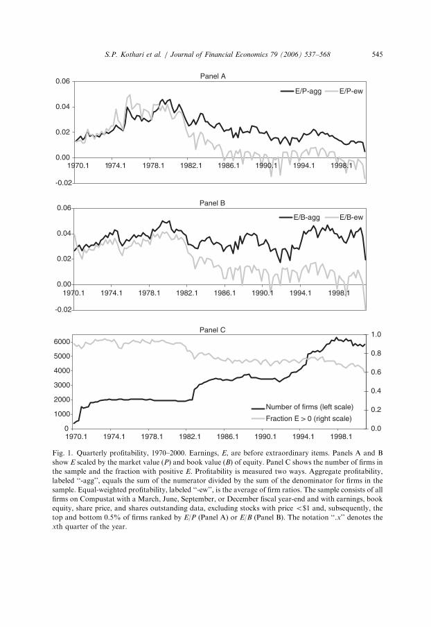
Fig. 1. Quarterly profitability, 1970–2000. Earnings, E, are before extraordinary items. Panels A and B
show E scaled by the market value (P) and book value (B) of equity. Panel C shows the number of firms in
the sample and the fraction with positive E. Profitability is measured two ways. Aggregate profitability,
labeled ‘‘-agg’’, equals the sum of the numerator divided by the sum of the denominator for firms in the
sample. Equal-weighted profitability, labeled ‘‘-ew’’, is the average of firm ratios. The sample consists of all
firms on Compustat with a March, June, September, or December fiscal year-end and with earnings, book
equity, share price, and shares outstanding data, excluding stocks with price o$1 and, subsequently, the
top and bottom 0.5% of firms ranked by E/P (Panel A) or E/B (Panel B). The notation ‘‘.x’’ denotes the
xth quarter of the year.
S.P. Kothari et al. / Journal of Financial Economics 79 (2006) 537–568 545

ARTICLE IN PRESS
Panel A
-0.60
-0.40
-0.20
0.00
0.20
0.40
0.60
1970.1 1974.1 1978.1 1982.1 1986.1 1990.1 1994.1 1998.1
dE/E-agg
Panel B
-0.010
-0.005
0.000
0.005
0.010
0.015
0.020
1970.1 1974.1 1978.1 1982.1 1986.1 1990.1 1994.1 1998.1
dE/P-vwdE/P-ew
Fig. 2. Seasonally differenced quarterly earnings, 1970–2000. Earnings, E, are measured before
extraordinary items. Seasonally differenced earnings, dE, are earnings this quarter minus earnings four
quarters ago. Panel A shows the growth rate of aggregate quarterly earnings, dE/E-agg, defined as the sum
of dE divided by the sum of earnings four quarters ago for firms in the sample. Panel B shows dE divided
by market value (P) at the end of quarter �4. In Panel B, the ratio is calculated for each firm and then
averaged; dE/P-vw is a value-weighted average and dE/P-ew is an equal-weighted average. The sample
consists of firms with a March, June, September, or December fiscal year-end and with earnings, book
equity, share price, and shares outstanding data on Compustat, excluding stocks with price below $1 and,
subsequently, the top and bottom 0.5% of firms ranked by dE/P. The notation ‘‘.x’’ denotes the xth
quarter of the year.
S.P. Kothari et al. / Journal of Financial Economics 79 (2006) 537–568546
Table 1 and Figs. 1 and 2 reveal several interesting facts. First, profitability since1970 has been fairly high. Average quarterly return on equity, E/B, is 4.13% for thevalue-weighted index and 1.90% for the equal-weighted index, implying annual E/Bof around 8–16%. This range is broad but brackets plausible estimates of the cost ofcapital. Fig. 1 shows that aggregate E/B declined in the early 1980s but has since

ARTICLE IN PRESS
S.P. Kothari et al. / Journal of Financial Economics 79 (2006) 537–568 547
remained stable or even increased. In contrast, aggregate earnings yield, E/P-agg,declined throughout the 1980s and 1990s, dropping from about 4% to about 1%quarterly. Comparing Panels A and B, the bull market of the 1980s and 1990s, not adecrease in profitability, seems to explain most of the drop in aggregate earningsyield.
Second, small stocks have much lower profitability than large stocks after 1980(see also Fama and French, 1995). In Fig. 1, equal-weighted E/P and E/B, which putmost weight on small firms, show a large decline in 1982 and subsequently a strikingdegree of fourth-quarter seasonality. Neither pattern is pronounced in the aggregateseries. Panel C shows that firms with negative earnings increase from less than 10%of the sample in 1970 to about 40% of the sample in 2000. In untabulated results, wefind little evidence that the patterns can be attributed to the expansion of the samplein 1982 (the sample jumps from 2007 to 2738 firms at the end of 1982; see Fig. 1,panel C). Firms existing prior to 1982 have earnings performance that is similar tonewly added firms.
Third, aggregate earnings exhibit substantial variability through time. Fig. 2 plotsthe growth rate of quarterly earnings, in Panel A, and earnings changes scaled bylagged price, in Panel B. Most of our tests focus on the price-scaled series because wecannot calculate growth rates for individual firms, since firm’s earnings are oftennegative. We can calculate an aggregate growth rate because aggregate earnings,before extraordinary items, are positive throughout the sample. (Aggregate netincome after extraordinary items does become negative in 1993. Also, as Table 1indicates, portfolio earnings become negative for subsamples of small and highbook-to-market stocks.)
Fig. 2 shows that earnings are volatile, with growth rates often more than 720%.The time-series properties appear to be stable during the sample, and seasonaldifferencing does a good job eliminating seasonality in earnings. The scaled-priceseries in Panel B, dE/P-ew and dE/P-vw, are highly correlated with each other andwith the earnings growth rate in Panel A (see also Table 2). The equal-weightedseries appears to be most variable. Earnings volatility is important for our later testsbecause, in the regressions, power hinges on the magnitude of earnings surprises (i.e.,for a given slope, higher earnings volatility implies greater power).
Finally, Table 1 reports statistics for the top and bottom terciles of stocks rankedby size and B/M. Comparing large and small firms, earnings levels are higher forlarge stocks but earnings growth is higher for small stocks. Comparing low-B/M andhigh-B/M firms, earnings levels and growth rates are both higher for low-B/M stocksif we scale by book equity, consistent with the standard value versus growthdichotomy. Growth is priced so highly, however, that the price-scaled measures, E/Pand dE/P, look as good or better for high-B/M stocks.
3.2. Autocorrelations
Table 3 explores the autocorrelation of seasonally differenced quarterly earnings.Firm-level results, in Panel A, are estimated for price-scaled earnings changes, whilemarket-level results, in Panel B, are estimated for dE/B-agg, dE/P-vw, and dE/P-ew.
ARTICLE IN PRESS
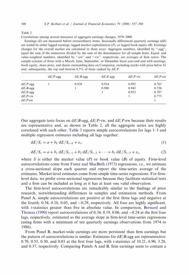
Table 2
Correlations among several measures of aggregate earnings changes, 1970–2000
Earnings (E) are measured before extraordinary items. Seasonally differenced quarterly earnings (dE)
are scaled by either lagged earnings, lagged market capitalization (P), or lagged book equity (B). Earnings
changes for the overall market are calculated in three ways: Aggregate numbers, identified by ‘‘-agg’’,
equal the sum of the numerator divided by the sum of the denominator for all sample firms. Equal- and
value-weighted numbers, identified by ‘‘-ew’’ and ‘‘-vw’’, respectively, are averages of firm ratios. The
sample consists of firms with a March, June, September, or December fiscal year-end and with earnings,
book equity, share price, and shares outstanding data on Compustat, excluding stocks with price below $1
and, subsequently, the top and bottom 0.5% of firms ranked by dE/P.
dE/P-agg dE/B-agg dE/E-agg dE/P-vw dE/P-ew
dE/P-agg 1 0.938 0.914 0.992 0.783
dE/B-agg 1 0.988 0.943 0.726
dE/E-agg 1 0.923 0.707
dE/P-vw 1 0.775
dE/P-ew 1
S.P. Kothari et al. / Journal of Financial Economics 79 (2006) 537–568548
Our aggregate tests focus on dE/B-agg, dE/P-vw, and dE/P-ew because their resultsare representative and, as shown in Table 2, all the aggregate series are highlycorrelated with each other. Table 3 reports simple autocorrelations for lags 1–5 andmultiple regression estimates including all lags together:
dE=St ¼ aþ bk dE=St�k þ et, (1)
dE=St ¼ aþ b1 dE=St�1 þ b2 dE=St�2 þ � � � þ b5 dE=St�5 þ et, (2)
where S is either the market value (P) or book value (B) of equity. Firm-levelautocorrelations come from Fama and MacBeth (1973) regressions, i.e., we estimatea cross-sectional slope each quarter and report the time-series average of theestimates. Market-level estimates come from simple time-series regressions. For firm-level data, we prefer cross-sectional regressions because they facilitate statistical testsand a firm can be included as long as it has at least one valid observation.
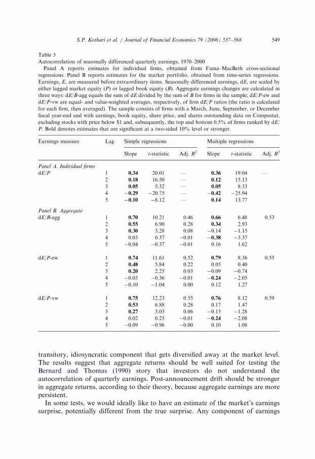
The firm-level autocorrelations are remarkably similar to the findings of priorresearch, notwithstanding differences in samples and estimation methods. FromPanel A, simple autocorrelations are positive at the first three lags and negative atthe fourth: 0.34, 0.18, 0.05, and �0.29, respectively. All four are highly significant,with t-statistics greater than five in absolute value. In comparison, Bernard andThomas (1990) report autocorrelations of 0.34, 0.19, 0.06, and �0.24 at the first fourlags, respectively, estimated as the average slope in firm-level time-series regressions(using firms with a minimum of ten quarterly earnings observations from 1974 to1986).
From Panel B, market-wide earnings are more persistent than firm earnings butthe pattern of autocorrelations is similar. Estimates for dE/B-agg are representative:0.70, 0.55, 0.30, and 0.03 at the first four lags, with t-statistics of 10.21, 6.90, 3.28,and 0.37, respectively. Comparing Panels A and B, firm earnings seem to contain a
ARTICLE IN PRESS
Table 3
Autocorrelation of seasonally differenced quarterly earnings, 1970–2000
Panel A reports estimates for individual firms, obtained from Fama–MacBeth cross-sectional
regressions. Panel B reports estimates for the market portfolio, obtained from time-series regressions.
Earnings, E, are measured before extraordinary items. Seasonally differenced earnings, dE, are scaled by
either lagged market equity (P) or lagged book equity (B). Aggregate earnings changes are calculated in
three ways: dE/B-agg equals the sum of dE divided by the sum of B for firms in the sample; dE/P-ew and
dE/P-vw are equal- and value-weighted averages, respectively, of firm dE/P ratios (the ratio is calculated
for each firm, then averaged). The sample consists of firms with a March, June, September, or December
fiscal year-end and with earnings, book equity, share price, and shares outstanding data on Compustat,
excluding stocks with price below $1 and, subsequently, the top and bottom 0.5% of firms ranked by dE/
P. Bold denotes estimates that are significant at a two-sided 10% level or stronger.
Earnings measure Lag Simple regressions Multiple regressions
Slope t-statistic Adj. R2 Slope t-statistic Adj. R2
Panel A. Individual firms
dE/P 1 0.34 20.01 — 0.36 19.04 —
2 0.18 16.50 — 0.12 15.13
3 0.05 5.32 — 0.05 8.33
4 �0.29 �20.75 — �0.42 �25.94
5 �0.10 �8.12 — 0.14 13.77
Panel B. Aggregate
dE/B-agg 1 0.70 10.21 0.46 0.66 6.48 0.53
2 0.55 6.90 0.28 0.34 2.93
3 0.30 3.28 0.08 �0.14 �1.15
4 0.03 0.37 �0.01 �0.38 �3.37
5 �0.04 �0.37 �0.01 0.16 1.62
dE/P-ew 1 0.74 11.61 0.52 0.79 8.36 0.55
2 0.48 5.84 0.22 0.05 0.40
3 0.20 2.25 0.03 �0.09 �0.74
4 �0.03 �0.36 �0.01 �0.24 �2.05
5 �0.10 �1.04 0.00 0.12 1.27
dE/P-vw 1 0.75 12.23 0.55 0.76 8.12 0.59
2 0.53 6.88 0.28 0.17 1.47
3 0.27 3.03 0.06 �0.15 �1.28
4 0.02 0.25 �0.01 �0.24 �2.08
5 �0.09 �0.96 �0.00 0.10 1.08
S.P. Kothari et al. / Journal of Financial Economics 79 (2006) 537–568 549
transitory, idiosyncratic component that gets diversified away at the market level.The results suggest that aggregate returns should be well suited for testing theBernard and Thomas (1990) story that investors do not understand theautocorrelation of quarterly earnings. Post-announcement drift should be strongerin aggregate returns, according to their theory, because aggregate earnings are morepersistent.
In some tests, we would ideally like to have an estimate of the market’s earningssurprise, potentially different from the true surprise. Any component of earnings

ARTICLE IN PRESS
S.P. Kothari et al. / Journal of Financial Economics 79 (2006) 537–568550
anticipated by investors would not affect current returns and would bias our slopeestimates toward zero. If investors believe earnings follow a seasonal random walk,earnings surprises are the same as earnings changes. If investors are rational, at aminimum we should take out the component of the earnings change that ispredictable based on past earnings. We use an AR1 model for this purpose becauseTable 3 indicates that it does a good job picking out the predictable component. Inmultiple regressions, few of the autocorrelations beyond lag 1 are significant and theincrease in R2 is modest (adding lags 2–5 increases the R2 from an average of 0.51 toan average of 0.56 for the three earnings series). Our tests also consider thepossibility that earnings are predictable using past returns.
4. The reaction to earnings surprises
Our main tests explore how the market reacts to aggregate earnings surprises,mirroring studies of post-earnings announcement drift in firm returns. We verifydrift for individual firms in our sample but find substantially different results inaggregate data.
4.1. Quarterly returns and earnings
In Table 4, we regress firm returns (Panel A) and market returns (Panel B) oncurrent and past earnings changes:
Rtþk ¼ aþ b dE=St þ etþk, (3)
where Rtþk is return for quarter tþ k and dE/St is seasonally differenced earnings forquarter t scaled by either the market value ðS ¼ PÞ or book value ðS ¼ BÞ of equity.Returns vary from k ¼ 0 to 4 quarters in the future. Here, k ¼ 0 refers to the quarterfor which earnings are measured and k ¼ 1 refers to the quarter in which earningsare typically announced. These quarters both measure the contemporaneous return-earnings association: The market learns much about a firm’s performance during themeasurement quarter, k ¼ 0, but earnings announcements clearly convey informa-tion to the market as well (see, e.g., Ball and Brown, 1968; Foster, 1977). Firmssometimes announce earnings more than three months after fiscal year-end, in whichcase k ¼ 2 also reflects the market’s reaction to new information. This effect shouldbe small in recent years.
Panel A reports Fama–MacBeth regressions for individual firms. Like priorstudies, we find that returns in quarters 0–3 have a strong positive association withearnings. The slopes for the measurement and announcement quarters, 0.61 and0.65, are largest and more than 30 standard errors above zero. The market alsoreacts strongly in quarters k ¼ 2 and 3, with slopes of 0.22 (t-statistic of 12.8) and0.11 (t-statistic of 6.1), respectively. Thus, investors appear to underreact to earningsnews, leading to post-announcement drift. The declining slopes for lags 2–4 line upwith the declining autocorrelation in earnings. As observed by Bernard and Thomas(1990), this suggests that investors do not understand earnings’ persistence.

ARTICLE IN PRESS
Table 4
Quarterly returns and earnings, 1970–2000
The table reports the slope estimate, t-statistic, and adjusted R2 when quarterly stock returns are
regressed on seasonally differenced quarterly earnings:
Rtþk ¼ aþ b dE=St þ etþk,
where dE is seasonally differenced earnings and S is either the market value (P) or book value (B) of
equity. Earnings are before extraordinary items. Rtþk varies from k ¼ 0 to 4 quarters in the future (k ¼ 0 is
the quarter for which earnings are measured; k ¼ 1 is the quarter in which earnings are typically
announced). Panel A reports estimates for individual firms, obtained from Fama–MacBeth regressions.
Panel B reports estimates for the market portfolio, obtained from time-series regressions. The market
return is the CRSP value-weighted index. dE/B-agg equals the sum of dE divided by the sum of B for all
firms in the earnings sample; dE/P-ew and dE/P-vw are equal- and value-weighted averages of firm dE/P
ratios. The earnings sample consists of firms with a March, June, September, or December fiscal year-end
and with earnings, book equity, share price, and shares outstanding data on Compustat, excluding stocks
with price o$1 and, subsequently, the top and bottom 0.5% of firms ranked by dE/P. Bold denotes
estimates that are significant at a two-sided 10% level or stronger.
Earnings measure k Earnings change Earnings surprise 1 Earnings surprise 2
Slope t-stat Adj. R2 Slope t-stat Adj. R2 Slope t-stat Adj. R2
Panel A. Individual firms
dE/P 0 0.61 32.83 — 0.49 28.47 — 0.50 28.67 —
1 0.65 30.76 — 0.67 33.80 — 0.67 34.23 —
2 0.22 12.78 — 0.22 12.93 — 0.22 13.77 —
3 0.11 6.10 — 0.12 6.90 — 0.11 7.51 —
4 0.01 0.52 — 0.03 1.81 — 0.04 2.30 —
Panel B. Aggregate
dE/B-agg 0 �2.35 �1.70 0.02 �0.37 �0.19 0.03 0.05 0.03 0.04
1 �3.39 �2.38 0.04 �7.19 �3.70 0.09 �6.87 �3.39 0.06
2 �0.35 �0.25 �0.01 1.13 0.56 �0.01 1.54 0.73 �0.01
3 �0.99 �0.71 �0.00 �0.25 �0.12 �0.01 0.42 0.20 �0.01
4 �1.12 �0.79 0.00 �2.65 �1.31 �0.00 �2.11 �0.98 �0.01
dE/P-ew 0 �1.42 �0.96 �0.00 2.68 1.27 0.05 3.16 1.47 0.05
1 �3.84 �2.60 0.05 �5.06 �2.42 0.05 �4.48 �2.01 0.04
2 �2.31 �1.58 0.01 �2.00 �0.94 0.00 �1.68 �0.74 0.01
3 �1.70 �1.16 0.00 0.74 0.35 0.01 1.74 0.77 0.04
4 �2.74 �1.89 0.02 �4.22 �1.98 0.02 �3.76 �1.62 0.03
dE/P-vw 0 �5.16 �2.27 0.03 �2.79 �0.82 0.03 �1.48 �0.43 0.05
1 �5.43 �2.38 0.04 �11.67 �3.57 0.08 �11.29 �3.27 0.07
2 �0.94 �0.42 �0.01 1.16 0.34 �0.01 2.13 0.59 �0.01
3 �1.62 �0.72 �0.00 �1.64 �0.48 �0.01 �0.37 �0.10 �0.01
4 �1.08 �0.48 �0.01 �3.79 �1.11 �0.00 �2.49 �0.68 �0.01
‘‘Earnings change’’ is the actual value of dE/S, ‘‘Earnings surprise 1’’ is the forecast error from an AR1
model, and ‘‘Earnings surprise 2’’ is the forecast error when dE/S is regressed on lagged dE/S and lagged
annual returns. In the latter two cases, the fitted value and forecast error from the forecasting regression
are both included in the second-stage return regression. ‘‘Adj. R2’’ measures the joint explanatory power of
both variables.
S.P. Kothari et al. / Journal of Financial Economics 79 (2006) 537–568 551

ARTICLE IN PRESS
S.P. Kothari et al. / Journal of Financial Economics 79 (2006) 537–568552
Panel B shows results for aggregate returns. We report estimates when CRSPvalue-weighted returns are regressed on either dE/B-agg, dE/P-ew, or dE/P-vw,using the simple earnings change, the forecast error from an AR1 model (Surprise 1),or the forecast error from a model that includes lagged earnings and lagged annualreturns (Surprise 2). The last measure uses past returns to take out more of theanticipated component of earnings.3 The panel shows two striking results: (1) thecontemporaneous relation between returns and earnings is significantly negative; and(2) past earnings have little power to predict future returns—if anything, thepredictive slopes are negative, opposite the predictions of behavioral models. Wediscuss these findings below.
4.1.1. Contemporaneous relation
Regardless of which earnings measure we use, market returns in the announcementquarter, k ¼ 1, correlate negatively with aggregate earnings. For simple earnings changes,the slopes range from �3.39 to �5.43 with t-statistics between �2.38 and �2.60. Theseestimates are probably conservative because any measurement error in earnings surprisesshould attenuate the slopes. If we take out the component of the earnings changepredicted by an AR1 model, the slopes for dE/B-agg and dE/P-vw more than double andtheir t-statistics jump to �3.70 and �3.57, respectively. The results are similar if weremove the component of earnings predicted by past returns. The negative announcementeffect is surprising and contrasts strongly with firm-level evidence.
Economically, the slope estimates for k ¼ 1 are fairly large. Earnings explain4–9% of quarterly returns and, using the point estimates in Table 4, a two-standard-deviation positive shock to earnings maps into a 4–6% decline in prices (the standarddeviation of earnings surprises from an AR1 model equals 0.42% for dE/B-agg,0.37% for dE/P-ew, and 0.23% for dE/P-vw). Historically, if earnings changes forany of the measures were in the bottom quartile of their distributions from 1970 to2000, the CRSP index return was about 7%. If earnings changes were in the topquartile, the CRSP index was essentially flat, increasing by about 1%.
Campbell (1991) shows that unexpected returns can be decomposed, mechanically,into cash-flow news and expected-return, or discount-rate, news. Thus, the priceimpact of earnings is determined by its covariance with each component. If goodearnings performance is accompanied by an increase in the discount rate, and if thelatter swamps the cash-flow news in earnings, then the overall correlation betweenearnings and returns can be negative.4
3We experimented with various return intervals and found that annual returns do a good job
summarizing the information in past prices. In the forecasting regression, the slope on lagged earnings is
similar to the autocorrelation reported in Table 3 and the slope on returns has a t-statistic of 2.07 for dE/
B-agg, 3.47 for dE/P-ew, and 3.17 for dE/P-vw. The R2s are slightly higher than for a simple AR1 model.4We take it for granted that earnings and cash flows are positively correlated. Table 3 suggests that
aggregate earnings shocks are permanent (earnings changes are positively autocorrelated for several
quarters and show no sign of long-term reversal) and, as such, should eventually lead to higher dividends
(Lintner, 1956; Campbell and Shiller, 1988a). We also emphasize that our results pertain to relatively
short-run earnings surprises, i.e., quarterly and annual. In the long run, prices and earnings should move
together.
ARTICLE IN PRESS
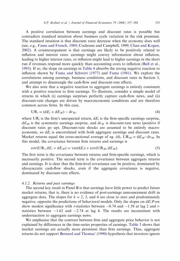
S.P. Kothari et al. / Journal of Financial Economics 79 (2006) 537–568 553
A positive correlation between earnings and discount rates is possible butcontradicts standard intuition about business cycle variation in the risk premium.The standard intuition is that discount rates decrease when the economy does well(see, e.g., Fama and French, 1989; Cochrane and Campbell, 1999; Chan and Kogan,2002). A counterargument is that earnings are likely to be positively related toinflation and interest rates: earnings might convey information about inflation,leading to higher interest rates, or inflation might lead to higher earnings in the shortrun if revenues respond more quickly than accounting costs to inflation (Ball et al.,1993). If so, the slope on earnings in Table 4 absorbs the strong negative reaction toinflation shown by Fama and Schwert (1977) and Fama (1981). We explore thecorrelations among earnings, business conditions, and discount rates in Section 5,and attempt to disentangle the cash-flow and discount-rate effects.
We also note that a negative reaction to aggregate earnings is entirely consistentwith a positive reaction to firm earnings. To illustrate, consider a simple model ofreturns in which (i) earnings surprises perfectly capture cash-flow news, and (ii)discount-rate changes are driven by macroeconomic conditions and are thereforecommon across firms. In this case,
URi ¼ ðdEi þ dEM Þ � drM , (4)
where URi is the firm’s unexpected return, dEi is the firm-specific earnings surprise,dEM is the systematic earnings surprise, and drM is discount-rate news (positive ifdiscount rates go up). Discount-rate shocks are assumed to be entirely macro-economic, so dEi is uncorrelated with both aggregate earnings and discount rates.Market returns equal the cross-sectional average of eg. (4), URM ¼ dEM�drM. Inthis model, the covariance between firm returns and earnings is
covðURi;dEi þ dEMÞ ¼ varðdEiÞ þ covðURM ;dEMÞ. (5)
The first term is the covariance between returns and firm-specific earnings, which isnecessarily positive. The second term is the covariance between aggregate returnsand earnings. It is clear that the firm-level covariance can be positive, dominated byidiosyncratic cash-flow shocks, even if the aggregate covariance is negative,dominated by discount-rate effects.
4.1.2. Returns and past earnings
The second key result in Panel B is that earnings have little power to predict futuremarket returns; that is, there is no evidence of post-earnings announcement drift inaggregate data. The slopes for k ¼ 2, 3, and 4 are close to zero and predominatelynegative, opposite the predictions of behavioral models. Only the slopes on dE/P-ewshow modest significance with t-statistics between �0.74 and �1.58 at lag 2 and t-statistics between �1.62 and �2.74 at lag 4. The results are inconsistent withunderreaction to aggregate earnings news.
We emphasize that the contrast between firm and aggregate price behavior is notexplained by differences in the time-series properties of earnings. Table 3 shows thatmarket earnings are actually more persistent than firm earnings. Thus, aggregatereturns do not support Bernard and Thomas’ (1990) hypothesis that investors ignore
ARTICLE IN PRESS
S.P. Kothari et al. / Journal of Financial Economics 79 (2006) 537–568554
the autocorrelation structure of earnings. Moreover, the positive relation betweenearnings and discount-rate changes implied by our k ¼ 1 slopes should make it easierto find post-announcement drift in returns: if earnings and discount-rate shocks arepositively related, earnings would be positively correlated with future returns even inthe absence of any underreaction.
4.2. Robustness checks
The aggregate results are rather surprising, so it seems worthwhile to consider afew robustness checks. The bottom line is that we find similar results for alternativedefinitions of earnings; each of the decades 1970s, 1980s, and 1990s; annualregressions; S&P 500 earnings going back to the 1930s; and size-sorted portfolios.
4.2.1. Alternative earnings variables
In addition to the three earnings series shown in Table 4, we ran regressions withaggregate dE scaled by lagged market values or lagged earnings. The results aresimilar to those in Table 4. For example, in regressions with aggregate earningsgrowth, dE/E, the t-statistics are �1.69 and �2.47 for k ¼ 0 and 1, respectively, andbetween �1.00 and �0.30 for the remaining lags. We find similar but somewhatweaker results if we use net income in place of earnings before extraordinary items.
4.2.2. Subperiods
To check whether the results are driven by one or two observations, or by returnsat the end of the sample, we repeat the tests for each of the decades 1970s, 1980s, and1990s. Again, the results are similar to those in Table 4. The slope coefficients onearnings changes are generally negative at all lags but not individually significantgiven the short sample in each decade. The coefficients on earnings surprises from anAR1 model are more significant. For example, using surprises based on dE/B-agg,the t-statistic at k ¼ 1 equals �1.95 for 1970–1979, �2.62 for 1980–1989, and �2.05for 1990–2000. Estimates for the other series are also negative, but not as significant.We never find evidence of post-announcement drift in aggregate returns.
4.2.3. Annual returns and earnings
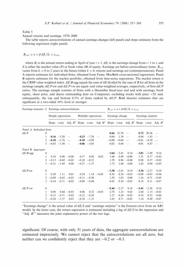
Table 5 replicates the analysis using annual data. We report return regressions forboth individual firms and the market, along with earnings autocorrelations. Thevariable definitions and data requirements are like those for the quarterly tests exceptthat the sample is restricted to firms with December fiscal year-ends (to make surethat fiscal years align). Annual returns are measured from May to the followingApril to control for delays in earnings announcements.
The time-series properties of annual earnings are consistent with prior studies (see,e.g., Ball and Watts, 1972; Brooks and Buckmaster, 1976). Earnings changes forindividual firms are negatively autocorrelated for two to three years, with t-statisticsas large as �7.58. At the same time, aggregate earnings are indistinguishable from arandom walk. Earnings changes for the overall market are positively autocorrelatedat lag 1 and negatively autocorrelated at lags 2 and 3, but none of the estimates is
ARTICLE IN PRESS
Table 5
Annual returns and earnings, 1970–2000
The table reports autocorrelations of annual earnings changes (left panel) and slope estimates from the
following regression (right panel):
Rtþk ¼ aþ b dE=St þ etþk,
where Rt is the annual return ending in April of year tþ 1, dEt is the earnings change from t�1 to t, and
S is either the market value (P) or book value (B) of equity. Earnings are before extraordinary items. Rtþk
varies from k ¼ 0 to 2 years in the future (when k ¼ 0, returns and earnings are contemporaneous). Panel
A reports estimates for individual firms, obtained from Fama–MacBeth cross-sectional regressions. Panel
B reports estimates for the market portfolio, obtained from time-series regressions. The market return is
the CRSP value-weighted index. dE/B-agg equals the sum of dE divided by the sum of B for all firms in the
earnings sample; dE/P-ew and dE/P-vw are equal- and value-weighted averages, respectively, of firm dE/P
ratios. The earnings sample consists of firms with a December fiscal-year end and with earnings, book
equity, share price, and shares outstanding data on Compustat, excluding stocks with price o$1 and,
subsequently, the top and bottom 0.5% of firms ranked by dE/P. Bold denotes estimates that are
significant at a two-sided 10% level or stronger.
Earnings measure k Earnings autocorrelations Rtþk ¼ aþ bdE=St þ etþk
Simple regressions Multiple regressions Earnings change Earnings surprise
Slope t-stat Adj. R2 Slope t-stat Adj. R2 Slope t-stat Adj. R2 Slope t-stat Adj. R2
Panel A. Individual firms
dE/P 0 0.66 21.59 — 0.72 20.56 —
1 �0.16 �5.58 — �0.23 �7.58 — 0.04 1.39 — 0.04 1.43 —
2 �0.10 �2.76 — �0.18 �4.99 �0.00 �0.04 — �0.01 �0.20 —
3 �0.03 �1.50 — �0.06 �3.05 0.02 0.64 — 0.01 0.47 —
Panel B. Aggregate
dE/B-agg 0 �3.64 �2.41 0.14 �3.81 �2.49 0.16
1 0.18 0.98 �0.00 0.17 0.88 0.02 1.60 0.99 �0.00 1.31 0.77 �0.02
2 �0.13 �0.69 �0.02 �0.10 �0.51 1.59 0.96 �0.00 0.98 0.57 �0.02
3 �0.31 �1.69 0.06 �0.27 �1.37 1.72 1.04 0.00 1.42 0.84 �0.05
dE/P-ew 0 �3.38 �2.41 0.14 �3.36 �2.27 0.10
1 0.20 1.11 0.01 0.24 1.14 �0.05 0.36 0.24 �0.03 �0.08 �0.05 �0.04
2 �0.09 �0.45 �0.03 �0.11 �0.50 1.59 1.03 0.00 1.16 0.71 �0.05
3 �0.14 �0.71 �0.02 �0.09 �0.44 0.85 0.54 �0.03 0.18 0.11 �0.07
dE/P-vw 0 �5.44 �2.57 0.16 �5.41 �2.58 0.18
1 0.08 0.44 �0.03 0.06 0.32 �0.03 2.78 1.23 0.02 2.64 1.15 �0.02
2 �0.13 �0.71 �0.02 �0.12 �0.58 1.27 0.54 �0.03 0.76 0.32 �0.06
3 �0.26 �1.37 0.03 �0.24 �1.21 1.65 0.71 �0.02 1.14 0.49 �0.07
‘‘Earnings change’’ is the actual value of dE/S and ‘‘earnings surprise’’ is the forecast error from an AR1
model. In the latter case, the return regression is estimated including a lag of dE/S in the regression and
‘‘Adj. R2’’ measures the joint explanatory power of the two lags.
S.P. Kothari et al. / Journal of Financial Economics 79 (2006) 537–568 555
significant. Of course, with only 31 years of data, the aggregate autocorrelations areestimated imprecisely. We cannot reject that the autocorrelations are all zero, butneither can we confidently reject that they are �0.2 or �0.3.

ARTICLE IN PRESS
S.P. Kothari et al. / Journal of Financial Economics 79 (2006) 537–568556
The return regressions in Table 5 largely reinforce our quarterly results. At thefirm level, returns and contemporaneous earnings are positively related, but there isno evidence of delayed reaction to earnings news. A simple underreaction storypredicts a positive slope on lagged earnings, while the Bernard and Thomas (1990)naı̈ve expectations model predicts a negative slope to match the autocorrelationstructure of earnings. It would be interesting to understand better why post-earningsannouncement drift does not show up at annual horizons.
The market-level regressions also match our quarterly results. Annual marketreturns are contemporaneously negatively correlated with all three earningsmeasures, defined using either the simple earnings change or residuals from anAR1 regression (which makes little difference). The adjusted R2s are substantial,between 10% and 18%, and the t-statistics range from �2.27 to �2.57 even thoughwe have only 31 annual observations. Further, lagged earnings exhibit no predictivepower for future annual returns. This result is consistent with both market efficiencyor the Bernard and Thomas (1990) naı̈ve expectations story, because marketearnings are not highly autocorrelated. Overall, the results confirm inferences fromquarterly regressions.
4.2.4. The S&P 500
Our main tests use Compustat data for two reasons: (1) to allow an easycomparison between firm and aggregate results, and (2) to ensure the quality andtiming of accounting information. At the same time, Compustat data restrict us to afairly short sample, 1970–2000. To check whether this period is special, we repeat thetests using earnings on the S&P 500 (and its predecessors) going back to 1936, theearliest year for which quarterly earnings data are available. We regress CRSPreturns on either the earnings growth rate, dE/E, or the earnings change scaled bylagged market value, dE/P. The data come from various issues of Standard andPoor’s Analyst’s Handbook.
As shown in Table 6, the results for 1970–2000 are similar to our earlierestimates. The slopes on dE/P at lags 0 and 1 are �5.00 and �4.78 (t-statistics of�2.28 and �2.16), respectively, compared with estimates in Table 4 of �5.16 and�5.43. More important, the negative reaction to earnings news shows up out-of-sample from 1936 to 1969 and in all of the time periods we consider. Prior to 1970,the negative price reaction is delayed, appearing most strongly at lags 1 and 2.This suggests that earnings news reached the market more slowly in the earlyperiod, perhaps because quarterly reports were less common (quarterlyreports were required by NYSE in 1939 and by the Securities and ExchangeCommission in 1970; see Leftwich et al., 1981). The slopes for k ¼ 2 are especiallystrong, with t-statistics between �2.10 and �2.42 for the various series. After 1956,when the index expanded to five hundred firms, the slopes on earnings changes dE/Eand dE/P are significant for k ¼ 0 and 1, with t-statistics between �1.94 and �2.55,and negative but not significant for the remaining lags. In short, the negativereaction to aggregate earnings news is not unique to either our time period or oursample of firms.

ARTICLE IN PRESS
Table 6
Quarterly returns and S&P 500 earnings, 1936–2000
The table reports the slope estimate and t-statistic when quarterly stock market returns are regressed on
seasonally differenced quarterly earnings for Standard and Poor’s (S&P) Composite Index:
Rtþk ¼ aþ b dE=St þ etþk,
where dE is seasonally differenced earnings and S is either lagged earnings (E, in panel A) or lagged
market value (P, in panel B) of the S&P 500 and its predecessors (the index was expanded to five hundred
firms in 1957). The regression is estimated over four sample periods: 1936–2000, 1957–2000, 1970–2000,
and 1936–1969. The market return is the CRSP value-weighted index, varying from k ¼ 0 to 4 quarters in
the future (k ¼ 0 is the quarter for which earnings are measured; k ¼ 1 is the quarter in which earnings are
typically announced). ‘‘Earnings change’’ is the actual value of dE/S and ‘‘earnings surprise’’ is the forecast
error from an AR1 model. In the latter case, the return regression is estimated including a lag of dE/S in
the regression. Bold denotes estimates that are significant at a two-sided 10% level.
k Earnings change Earnings surprise
1936–2000 1957–2000 1970–2000 1936–1969 1936–2000 1957–2000 1970–2000 1936–1969
Panel A. Earnings growth, dE/E
Slope 0 �0.03 �0.06 �0.06 �0.00 0.02 �0.03 �0.04 0.06
1 �0.06 �0.08 �0.07 �0.06 �0.06 �0.11 �0.12 �0.03
2 �0.04 �0.01 �0.01 �0.06 �0.04 0.01 0.02 �0.08
3 �0.02 �0.03 �0.02 �0.02 �0.01 �0.03 �0.01 �0.00
4 �0.03 �0.02 �0.02 �0.03 �0.04 �0.03 �0.03 �0.04
t-stat 0 �1.12 �1.94 �1.72 �0.04 0.73 �0.75 �0.84 1.68
1 �2.85 �2.33 �1.91 �2.18 �2.24 �2.58 �2.64 �0.93
2 �1.73 �0.39 �0.18 �2.31 �1.48 0.13 0.42 �2.42
3 �0.93 �0.93 �0.63 �0.68 �0.25 �0.82 �0.28 �0.00
4 �1.22 �0.51 �0.58 �1.13 �1.40 �0.73 �0.69 �1.25
Panel B. Earnings changes scaled by lagged price, dE/P
Slope 0 �1.39 �4.82 �5.00 0.20 0.49 �2.84 �3.51 2.10
1 �2.70 �4.95 �4.78 �1.83 �2.21 �7.23 �8.35 �0.07
2 �2.15 �1.36 �0.93 �2.85 �2.56 0.04 0.89 �4.01
3 �1.03 �2.21 �1.74 �0.69 �0.78 �4.01 �2.83 0.12
4 �0.94 �0.09 �0.11 �1.30 �1.71 �1.20 �1.03 �1.97
t-stat 0 �1.18 �2.49 �2.28 0.14 0.32 �1.10 �1.19 1.21
1 �2.30 �2.55 �2.16 �1.34 �1.45 �2.77 �2.91 �0.04
2 �1.82 �0.69 �0.43 �2.10 �1.67 0.01 0.30 �2.31
3 �0.87 �1.13 �0.80 �0.50 �0.51 �1.52 �0.96 0.07
4 �0.79 �0.04 �0.05 �0.94 �1.11 �0.45 �0.35 �1.12
S.P. Kothari et al. / Journal of Financial Economics 79 (2006) 537–568 557
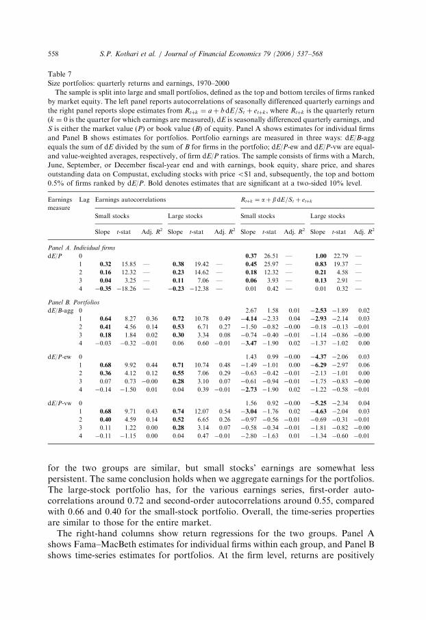
4.2.5. Size portfolios
As a final check, Table 7 repeats the analysis separately for big and small stocks,defined as the top and bottom terciles of firms ranked by market equity (these testsuse our main Compustat sample). Earnings autocorrelations, in the left columns,have the same patterns as our earlier estimates. At the firm level, autocorrelations arepositive at lags 1–3 and negative at lag 4 for both small and large stocks. Estimates
ARTICLE IN PRESS
Table 7
Size portfolios: quarterly returns and earnings, 1970–2000
The sample is split into large and small portfolios, defined as the top and bottom terciles of firms ranked
by market equity. The left panel reports autocorrelations of seasonally differenced quarterly earnings and
the right panel reports slope estimates from Rtþk ¼ aþ bdE=St þ etþk, where Rtþk is the quarterly return
(k ¼ 0 is the quarter for which earnings are measured), dE is seasonally differenced quarterly earnings, and
S is either the market value (P) or book value (B) of equity. Panel A shows estimates for individual firms
and Panel B shows estimates for portfolios. Portfolio earnings are measured in three ways: dE/B-agg
equals the sum of dE divided by the sum of B for firms in the portfolio; dE/P-ew and dE/P-vw are equal-
and value-weighted averages, respectively, of firm dE/P ratios. The sample consists of firms with a March,
June, September, or December fiscal-year end and with earnings, book equity, share price, and shares
outstanding data on Compustat, excluding stocks with price o$1 and, subsequently, the top and bottom
0.5% of firms ranked by dE/P. Bold denotes estimates that are significant at a two-sided 10% level.
Earnings
measure
Lag Earnings autocorrelations Rtþk ¼ aþ bdE=St þ etþk
Small stocks Large stocks Small stocks Large stocks
Slope t-stat Adj. R2 Slope t-stat Adj. R2 Slope t-stat Adj. R2 Slope t-stat Adj. R2
Panel A. Individual firms
dE/P 0 0.37 26.51 — 1.00 22.79 —
1 0.32 15.85 — 0.38 19.42 — 0.45 25.97 — 0.83 19.37 —
2 0.16 12.32 — 0.23 14.62 — 0.18 12.32 — 0.21 4.58 —
3 0.04 3.25 — 0.11 7.06 — 0.06 3.93 — 0.13 2.91 —
4 �0.35 �18.26 — �0.23 �12.38 — 0.01 0.42 — 0.01 0.32 —
Panel B. Portfolios
dE/B-agg 0 2.67 1.58 0.01 �2.53 �1.89 0.02
1 0.64 8.27 0.36 0.72 10.78 0.49 �4.14 �2.33 0.04 �2.93 �2.14 0.03
2 0.41 4.56 0.14 0.53 6.71 0.27 �1.50 �0.82 �0.00 �0.18 �0.13 �0.01
3 0.18 1.84 0.02 0.30 3.34 0.08 �0.74 �0.40 �0.01 �1.14 �0.86 �0.00
4 �0.03 �0.32 �0.01 0.06 0.60 �0.01 �3.47 �1.90 0.02 �1.37 �1.02 0.00
dE/P-ew 0 1.43 0.99 �0.00 �4.37 �2.06 0.03
1 0.68 9.92 0.44 0.71 10.74 0.48 �1.49 �1.01 0.00 �6.29 �2.97 0.06
2 0.36 4.12 0.12 0.55 7.06 0.29 �0.63 �0.42 �0.01 �2.13 �1.01 0.00
3 0.07 0.73 �0.00 0.28 3.10 0.07 �0.61 �0.94 �0.01 �1.75 �0.83 �0.00
4 �0.14 �1.50 0.01 0.04 0.39 �0.01 �2.73 �1.90 0.02 �1.22 �0.58 �0.01
dE/P-vw 0 1.56 0.92 �0.00 �5.25 �2.34 0.04
1 0.68 9.71 0.43 0.74 12.07 0.54 �3.04 �1.76 0.02 �4.63 �2.04 0.03
2 0.40 4.59 0.14 0.52 6.65 0.26 �0.97 �0.56 �0.01 �0.69 �0.31 �0.01
3 0.11 1.22 0.00 0.28 3.14 0.07 �0.58 �0.34 �0.01 �1.81 �0.82 �0.00
4 �0.11 �1.15 0.00 0.04 0.47 �0.01 �2.80 �1.63 0.01 �1.34 �0.60 �0.01
S.P. Kothari et al. / Journal of Financial Economics 79 (2006) 537–568558
for the two groups are similar, but small stocks’ earnings are somewhat lesspersistent. The same conclusion holds when we aggregate earnings for the portfolios.The large-stock portfolio has, for the various earnings series, first-order auto-correlations around 0.72 and second-order autocorrelations around 0.55, comparedwith 0.66 and 0.40 for the small-stock portfolio. Overall, the time-series propertiesare similar to those for the entire market.
The right-hand columns show return regressions for the two groups. Panel Ashows Fama–MacBeth estimates for individual firms within each group, and Panel Bshows time-series estimates for portfolios. At the firm level, returns are positively
ARTICLE IN PRESS
S.P. Kothari et al. / Journal of Financial Economics 79 (2006) 537–568 559
related to both concurrent and past earnings. Prices initially react most strongly forlarge firms, with point estimates of 1.00 and 0.83 for k ¼ 0 and 1 (t-statistics of 22.8and 19.4), respectively, compared with slopes of 0.37 and 0.45 for small stocks. Thestronger reaction for large firms is surprising because the earnings processes for thetwo groups are similar and investors are likely to have better prior informationabout large firms’ earnings. Post-announcement drift is about the same for small andlarge stocks, which again is surprising because the groups differ in many dimensionsthat might affect the market’s reaction to earnings news, including averageprofitability, liquidity, and earnings volatility.
The portfolio-level tests, in Panel B, suggest interesting differences across groups.Large stocks provide stronger evidence that portfolio returns and concurrentearnings are negatively correlated. The slopes for the large-stock portfolio aresignificantly negative for both k ¼ 0 and 1, with t-statistics between –1.89 and –2.97,while the slopes for small stocks are significantly negative only at k ¼ 1. In terms of alead-lag relation, small stocks provide the only evidence that portfolio earningspredict (negatively) future returns. The slopes at lags 2–4 are all negative, withsignificance at lag 4 for two earnings measures, dE/B-agg and dE/P-ew (t-statistics of�1.90 and �2.36, respectively). These results are generally consistent with ourmarket-level regressions.
The portfolio evidence suggests several conclusions. First, earnings are mostpersistent for the large-stock portfolio, yet the market reacts most negatively to itsearnings news, a combination that is puzzling from a cash-flow perspective. Itsuggests that large-stock earnings are more strongly correlated with discount rates.Second, the small-stock portfolio provides the most reliable evidence of marketinefficiency, in that earnings changes predict returns four quarters in the future. Thenegative relation seems to indicate market overreaction, except that the con-temporaneous relation between returns and earnings is flat. None of the portfolioresults lines up with behavioral theories, either the Bernard and Thomas (1990)naı̈ve-investor model or an underreaction story.
5. Earnings, business conditions, and discount rates
Our return regressions establish two key results: (1) aggregate earnings and stockreturns are contemporaneously negatively related; and (2) earnings surprises containlittle information about future returns. To better understand these results, weexplore the relations among earnings, business conditions, and discount rates. Weare particularly interested in whether movements in discount-rate proxies can explainthe contemporaneous return-earnings association.
5.1. Framework
Campbell (1991) provides a convenient framework for thinking aboutthese issues. In particular, he shows that returns Rt can be decomposed into

ARTICLE IN PRESS
S.P. Kothari et al. / Journal of Financial Economics 79 (2006) 537–568560
three components.
Rt ¼ rt þ Zd;t � Zr;t, (6)
where rt is the expected return for period t, Zd,t is the shock to expected dividends,and Zr;t is the shock to expected returns (the last component has a negative signbecause an increase in expected returns reduces the current price).5 Eq. (6) impliesthat earnings’ covariance with returns depends on its covariances with rt, Zd;t, and�Zr;t. If we have a good proxy for unexpected earnings, dEt, the covariance with rt isnecessarily zero, so Eq. (6) implies
covðdEt;RtÞ ¼ covðdEt; Zd;tÞ � covðdEt; Zr;tÞ. (7)
The first term is positive as long as higher earnings are associated with higherdividends. But the overall covariance can be negative, as we find in the data, if higherearnings are associated with an increase in expected returns, i.e., if cov(dEt, Zr;t) ispositive.
Assuming investors are rational, expected returns are the same as discount rates.Thus, the correlation between dEt and Zr;t suggests that discount rates rise whenearnings are strong (see also Lettau and Ludvigson, 2004). One possibility is thathigh earnings lead to higher real or nominal interest rates. The negative price impactof higher real interest rates is clear, but Modigliani and Cohn (1979) argue thatprices react even to purely nominal interest-rate changes because investorsmistakenly discount real earnings at nominal rates (see Nissim and Penman, 2003;Campbell and Vuolteenaho, 2004, for recent evidence). On the other hand, financetheory suggests that the risk premium should be countercyclical and, thus, negativelyrelated to earnings, opposite the effect implied by our regressions. Countercyclicalmovements in the equity premium might arise if investors try to smoothconsumption (see, e.g., Lucas, 1978) or if aggregate risk aversion varies over thebusiness cycle (see, e.g., Campbell and Cochrane, 1999; Chan and Kogan, 2002).6
We attempt to isolate these effects by including discount-rate proxies in theregressions. Our hope is to measure the marginal impact of an earnings surprise aftercontrolling for discount-rate effects.
5.2. Earnings and business conditions
Table 8 reports correlations among earnings, economic activity, and severaldiscount-rate proxies. Our measures of economic activity include the growth rates ofgross domestic product (GDP), industrial production (IPROD), and personal
5Formally, Zd;t ¼P1
k¼0 rkDEtdtþk and Zr;t ¼
P1k¼1 r
kDEthtþk, where DEt is the change in expectation
from t�1 to t, dt is the log dividend growth rate, ht is the log stock return, and r is a number close to one
determined by the asset’s average dividend yield. The decomposition is only approximate.6This is not to say that pro-cyclical variation in the discount rate is impossible. Cochrane (2001), for
example, observes that discount rates should covary positively with expected growth rates (i.e., be pro-
cyclical) if investors have constant relative risk aversion greater than one (see also Yan, 2004). The
intuition is that, when growth rates are high, investors naturally want to consume more today and, in
equilibrium, have to be induced to save through higher rates of return.

ARTICLE IN PRESS
Table 8
Earnings and the macroeconomy, 1970–2000
The table reports correlations between seasonally differenced quarterly earnings and various
macroeconomic series. Panel A shows simple correlations and Panel B shows regression coefficients (t-
statistics in parentheses). E is earnings before extraordinary items. dE is seasonally differenced quarterly
earnings. P is the market value and B is the book value of equity. dE/B-agg equals the sum of dE divided
by the sum of B for firms in the sample; dE/P-ew and dE/P-vw are equal- and value-weighted averages of
firm dE/P ratios. TBILL is the one-year T-bill rate. TERM is the yield spread between ten-year T-bonds
and one-year T-bills. DEF is the yield spread between Baa- and Aaa-rated corporate bonds. SENT is
consumer sentiment from the University of Michigan Survey Research Center, available from 1979–2000.
GDP and CONS are per capita growth rates of gross domestic product and personal consumption,
respectively. IPROD is growth in industrial production. The prefix D denotes four quarter changes in the
variables. Real dE/B and dE/P are calculated using inflation-adjusted earnings, book values, and market
values; GDP and CONS are measured as nominal or real growth rates to match the definition of dE/B and
dE/P, while TBILL, TERM, and DEF are always nominal rates. The earnings sample consists of firms
with a March, June, September, or December fiscal year-end and with earnings, book equity, share price,
and shares outstanding data on Compustat, excluding stocks with price below $1 and, subsequently, the
top and bottom 0.5% of firms ranked by dE/P. Bold denotes regression slope estimates that are significant
at a two-sided 10% level.
Nominal dE Real dE
dE/B-agg dE/P-ew dE/P-vw dE/B-agg dE/P-ew dE/P-vw
Panel A. Correlations
DTBILL 0.579 0.395 0.610 0.491 0.322 0.505
DTERM �0.469 �0.363 �0.532 �0.464 �0.366 �0.535
DDEF �0.325 �0.526 �0.360 �0.420 �0.635 �0.488
DSENT 0.185 0.392 0.124 0.243 0.437 0.196
GDP 0.475 0.574 0.566 0.607 0.668 0.681
IPROD 0.605 0.670 0.656 0.677 0.751 0.754
CONS 0.363 0.490 0.444 0.485 0.603 0.535
Panel B. dEt ¼ aþ bDTBILLt þ gDTERMt þ lDDEF t þ rdEt�1 þ �DTBILL 0.09 0.03 0.04 0.06 0.02 0.02
(3.29) (1.16) (2.80) (2.36) (0.87) (1.78)
DTERM 0.03 0.01 �0.01 0.02 �0.00 �0.02
(0.65) (0.16) (�0.26) (0.35) (�0.04) (�0.75)
DDEF �0.32 �0.36 �0.20 �0.36 �0.45 �0.24
(�3.38) (�3.63) (�3.87) (�3.82) (�4.64) (�4.72)
dEt�1 0.51 0.57 0.55 0.54 0.49 0.55
(6.49) (7.36) (8.00) (7.00) (6.13) (8.30)
Adjusted R2 0.54 0.56 0.64 0.54 0.58 0.64
Adjusted R2 without AR1 0.38 0.37 0.44 0.36 0.45 0.44
S.P. Kothari et al. / Journal of Financial Economics 79 (2006) 537–568 561
consumption (CONS). Our discount-rate proxies include the one-year T-bill rate, theyield spread between ten-year and one-year T-bonds (TERM), and the yield spreadbetween low-grade and high-grade corporate debt (DEF). The latter two proxies aremotivated by Fama and French’s (1989) evidence that variables similar to DEF andTERM capture movements in expected stock and bond returns over the businesscycle. We exclude valuation ratios, such as dividend yield, from our set of proxiesbecause they are tied mechanically to prices (and we wish to test whether the proxies
ARTICLE IN PRESS
S.P. Kothari et al. / Journal of Financial Economics 79 (2006) 537–568562
explain price changes). Finally, we also report correlations for the University ofMichigan’s consumer sentiment index. The variables are all measured as annualchanges or growth rates ending in the quarter that earnings are measured.
Panel A shows simple correlations between earnings and the macro-variables. Notsurprisingly, earnings are strongly related to the growth measures, GDP, IPROD,and CONS. Earnings are most closely tied to industrial production, with correlationsbetween 0.60 and 0.75 for the various earnings series. Co-movement with GDP andCONS is somewhat weaker and, in unreported tests, we find that IPROD subsumesthe correlation with the other two variables.
The behavior of discount rates is more important for our purposes. Earnings arestrongly positively correlated with DTBILL (estimates between 0.32 and 0.61) andnegatively correlated with DTERM and DDEF (estimates between �0.33 and�0.64). The correlation with DTBILL suggests that higher earnings are associatedwith higher discount rates, but the correlations with DTERM and DDEF have thewrong sign if, as Fama and French (1989) find, TERM and DEF are positivelyrelated to the equity premium. It is interesting that DEF, a proxy for bankruptcyrisk, is most closely tied to the performance of smaller stocks, measured by the equal-weighted earnings series. Also, earnings are weakly positively related to consumersentiment. Untabulated results show that DSENT is positively related to returns(0.39 in quarterly data), so its correlation with earnings has the wrong sign forexplaining why the market reacts negatively to earnings news.
Our tests below ask whether changes in discount rates can explain the correlationbetween returns and earnings. An easy way to do this is to break earnings into acomponent related to discount-rate news and an orthogonal component by firstregressing earnings on the discount-rate proxies. We then include both componentsin the second-stage return regression. In the second-stage regression, the slope on theorthogonal component is identical to the slope on earnings if we directly includeDTBILL, DTERM, and DDEF in the regression; the two-stage approach simplyeases the presentation and interpretation of the results.
Table 8, Panel B, shows the first-stage regression of earnings on the discount-rateproxies and an AR1 term (to soak up residual autocorrelation remaining aftercontrolling for discount rates). DTBILL and DDEF are both highly significant anddrive out any correlation between earnings and DTERM. Like the simplecorrelations, the slopes on DTBILL are significantly positive except in regressionswith the equal-weighted earnings series (for that series, dE/P-ew, the slope becomesmarginally significant if DTERM is dropped from the regression). The slopes onDEF are all significantly negative. Collectively, the three discount-rate proxiesexplain about 40% of the volatility in earnings changes, or between 50% and 60%together with the AR1 term.
In the tests below, we modify the first-stage regression slightly to obtain the fittedvalue and residual used in the return regressions. In particular, we have to take astand on when to measure changes in the discount-rate proxies. The regressions useannual changes measured over the same interval as the earnings change (from t�4 tot). Most of the annual change is known prior to t and, in an efficient market, shouldhave little impact on subsequent returns. Therefore, a better choice might be to use

ARTICLE IN PRESS
S.P. Kothari et al. / Journal of Financial Economics 79 (2006) 537–568 563
the quarterly change in the quarter for which earnings are measured, or in thequarter during which earnings are announced. We find similar results using all threespecifications. In the reported tests, we use changes in the discount-rate proxies in thequarter that earnings are measured. The estimates from the first stage are generallyconsistent with those in Table 8. TBILL and DEF both drop in significance, whilethe AR1 term becomes relatively more important.
5.3. Returns, earnings, and discount rates
Table 9 reports the second-stage regressions of returns on current and pastearnings surprises. The projection of earnings on the discount-rate proxies and AR1term is labeled ‘‘Fitted dE/S’’ and the orthogonal component is labeled ‘‘ResidualdE/S.’’ The slope on Residual dE/S measures the marginal impact of an earningssurprise after controlling for discount rates.
Our discount-rate proxies only partially explain why the market reacts negativelyto good earnings news. The slopes on Residual dE/S are typically less negative, ormore positive, than the corresponding slopes in Table 4. But the most importantfinding is that returns in the announcement quarter, k ¼ 1, remain negativelycorrelated with earnings news, with t-statistics on Residual dE/S between �1.93 and�3.17. Table 9 also provides no evidence of post-earnings announcement drift inaggregate returns. Thus, our discount-rate proxies do not eliminate the negativereaction to earnings news or change our conclusions about post-announcement drift.
Alternative specifications for discount-rate changes, in the first-stage regressionsthat provide Residual dE/S, give similar results. If we measure DTBILL, DTERM,and DDEF in the announcement instead of measurement quarter, the t-statistics onResidual dE/S for k ¼ 1 are �3.33, �1.90, and �3.05 for the three earnings series. Ifwe instead use annual changes in TBILL, TERM, and DEF, as in Table 8, the t-statistics for k ¼ 1 are �2.33, �1.65, and �2.23.
5.3.1. Annual returns
Table 10 repeats the analysis using annual returns and earnings. In unreportedfirst-stage regressions, only T-bill rates are significant when used together withTERM, DEF, and an AR1 term (like returns, the discount-rate proxies are laggedfour months relative to annual earnings). DTBILL alone explains more than 50% ofannual earnings changes. For this reason, we use DTBILL as the only proxy fordiscount-rate news in Table 10.
The table shows two key results. First, movements in interest rates largely explainthe negative reaction to earnings news in annual data. The slopes on Residual dE/Sfor lag 0 are roughly one standard error below zero, compared with t-statisticsaround �2.5 using raw earnings changes (see Table 5). Thus, prices seem to reactnegatively to annual earnings news because high earnings are tied to high interestrates. But the point estimates on Residual dE/S remain negative, so DTBILL doesnot fully remove the discount-rate effects in earnings.
Second, earnings are positively correlated with returns in the subsequent yearðk ¼ 1Þ. The slope is positive for all three earnings series, and significant for both dE/

ARTICLE IN PRESS
Table 9
Quarterly returns and earnings, controlling for discount rates, 1970–2000
The table reports slope estimates when quarterly stock returns are regressed on seasonally differenced
quarterly earnings broken into two components:
Rtþk ¼ aþ b Fitted dE=St þ g Residual dE=St þ etþk ;
where dE is seasonally differenced earnings, S is either the market value (P) or book value (B) of equity,
and the two components of dE/S are obtained from the regression
dE=St ¼ aþ b DTBILLt þ g DTERMt þ l DDEFt þ r dE=St�1 þ �t.
Fitted dE/S is the fitted value from this regression and Residual dE/S is the residual. The variables
DTBILL, DTERM, and DDEF are one-quarter changes in the variables, measured in the quarter of
earnings measurement. Earnings are before extraordinary items. Rtþk varies from k ¼ 0 to 4 quarters in
the future (k ¼ 0 is the quarter for which earnings are measured). Rt is the return on the CRSP value-
weighted index. dE/B-agg equals the sum of dE divided by the sum of B for all firms in the earnings
sample; dE/P-ew and dE/P-vw are equal- and value-weighted averages, respectively, of firm dE/P ratios.
The earnings sample consists of firms with a March, June, September, or December fiscal year-end and
with earnings, book equity, share price, and shares outstanding data on Compustat, excluding stocks with
price o$1 and, subsequently, the top and bottom 0.5% of firms ranked by dE/P. Bold denotes estimates
that are significant at a two-sided 10% level or stronger.
Earnings measure k Fitted dE/S Residual dE/S Adj. R2
Slope t-stat Slope t-stat
dE/B-agg 0 �6.29 �3.39 1.87 0.96 0.08
1 �1.50 �0.83 �6.66 �3.17 0.07
2 �2.25 �1.21 2.61 1.21 0.01
3 �1.22 �0.65 �0.52 �0.24 �0.01
4 0.11 0.06 �2.50 �1.15 �0.01
dE/P-ew 0 �5.92 �3.32 5.65 2.51 0.11
1 �3.80 �2.11 �4.48 �1.93 0.05
2 �3.06 �1.68 �0.69 �0.29 0.01
3 �3.41 �1.87 1.34 0.57 0.02
4 �1.71 �0.93 �4.30 �1.81 0.02
dE/P-vw 0 �9.24 �3.24 1.15 0.32 0.07
1 �2.79 �1.00 �10.91 �3.06 0.06
2 �3.13 �1.10 3.30 0.90 0.00
3 �1.25 �0.44 �1.99 �0.54 �0.01
4 0.47 0.16 �3.28 �0.89 �0.01
S.P. Kothari et al. / Journal of Financial Economics 79 (2006) 537–568564
B-agg (t-statistic of 1.78) and dE/P-vw (t-statistic of 2.25). The estimate for dE/P-vwis economically large. An increase in Residual dE/P-vw by two standard deviations(2� 0.84%) maps into a 13.1% increase in expected return. Residual dE/P-vwexplains more than 10% of the variation in next year’s return. These results providethe first evidence that aggregate prices underreact to earnings news, but they are alsoconsistent with our argument that high earnings are associated with higher discount
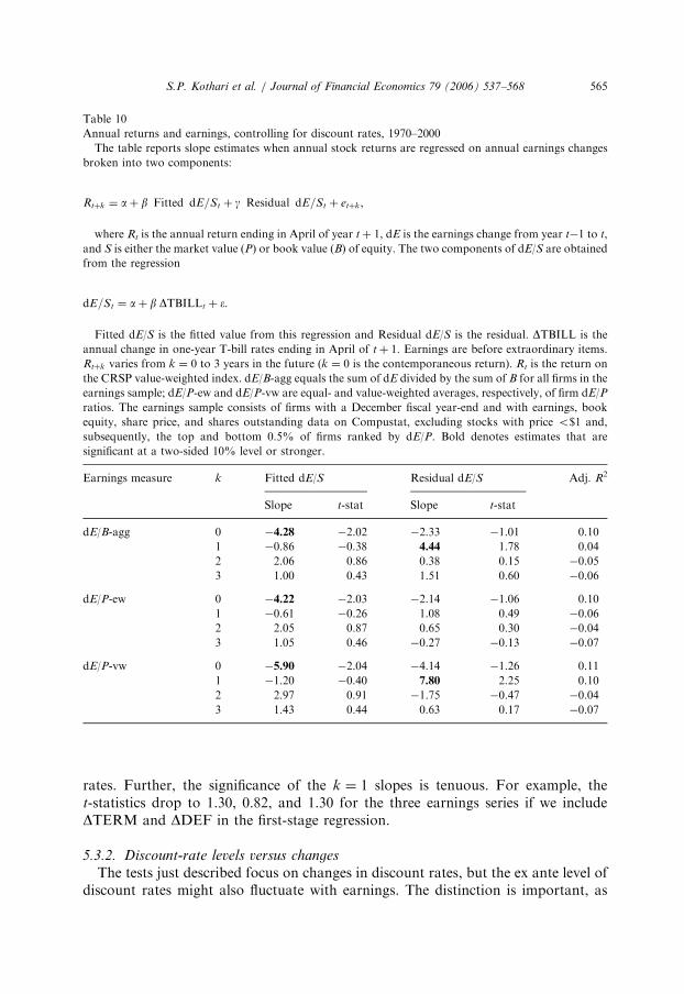
ARTICLE IN PRESS
Table 10
Annual returns and earnings, controlling for discount rates, 1970–2000
The table reports slope estimates when annual stock returns are regressed on annual earnings changes
broken into two components:
Rtþk ¼ aþ b Fitted dE=St þ g Residual dE=St þ etþk,
where Rt is the annual return ending in April of year tþ 1, dE is the earnings change from year t�1 to t,
and S is either the market value (P) or book value (B) of equity. The two components of dE/S are obtained
from the regression
dE=St ¼ aþ b DTBILLt þ �.
Fitted dE/S is the fitted value from this regression and Residual dE/S is the residual. DTBILL is the
annual change in one-year T-bill rates ending in April of tþ 1. Earnings are before extraordinary items.
Rtþk varies from k ¼ 0 to 3 years in the future (k ¼ 0 is the contemporaneous return). Rt is the return on
the CRSP value-weighted index. dE/B-agg equals the sum of dE divided by the sum of B for all firms in the
earnings sample; dE/P-ew and dE/P-vw are equal- and value-weighted averages, respectively, of firm dE/P
ratios. The earnings sample consists of firms with a December fiscal year-end and with earnings, book
equity, share price, and shares outstanding data on Compustat, excluding stocks with price o$1 and,
subsequently, the top and bottom 0.5% of firms ranked by dE/P. Bold denotes estimates that are
significant at a two-sided 10% level or stronger.
Earnings measure k Fitted dE/S Residual dE/S Adj. R2
Slope t-stat Slope t-stat
dE/B-agg 0 �4.28 �2.02 �2.33 �1.01 0.10
1 �0.86 �0.38 4.44 1.78 0.04
2 2.06 0.86 0.38 0.15 �0.05
3 1.00 0.43 1.51 0.60 �0.06
dE/P-ew 0 �4.22 �2.03 �2.14 �1.06 0.10
1 �0.61 �0.26 1.08 0.49 �0.06
2 2.05 0.87 0.65 0.30 �0.04
3 1.05 0.46 �0.27 �0.13 �0.07
dE/P-vw 0 �5.90 �2.04 �4.14 �1.26 0.11
1 �1.20 �0.40 7.80 2.25 0.10
2 2.97 0.91 �1.75 �0.47 �0.04
3 1.43 0.44 0.63 0.17 �0.07
S.P. Kothari et al. / Journal of Financial Economics 79 (2006) 537–568 565
rates. Further, the significance of the k ¼ 1 slopes is tenuous. For example, thet-statistics drop to 1.30, 0.82, and 1.30 for the three earnings series if we includeDTERM and DDEF in the first-stage regression.
5.3.2. Discount-rate levels versus changes
The tests just described focus on changes in discount rates, but the ex ante level ofdiscount rates might also fluctuate with earnings. The distinction is important, as
ARTICLE IN PRESS
S.P. Kothari et al. / Journal of Financial Economics 79 (2006) 537–568566
seen in Eq. (6): Rt ¼ rt þ Zd;t � Zr;t. The discount-rate level, rt, enters with a positivesign, but the discount-rate shock, Zr;t, enters with a negative sign. Thus, to explain anegative correlation with returns, earnings could be negatively correlated withdiscount-rate levels or positively correlated with discount-rate shocks. Theinterpretation of our results clearly depends on which is true.
We believe the results tell us principally about discount-rate shocks for severalreasons. First, if dEt is a good proxy for unexpected earnings, it must be uncorrelatedwith anything known prior to t, including rt. Our evidence in Section 3 suggests thata large fraction of dEt is, in fact, unexpected: dEt is quite volatile and time-seriesmodels explain only half of its variability. Moreover, when we remove thepredictable component to get a better proxy for unexpected earnings, the negativecorrelation with returns becomes stronger (Table 4). This suggests that unexpectedearnings, which can only be correlated with Zr;t, drive our results.
Second, dEt explains a large fraction of quarterly and annual returns: 4% to 9% ofquarterly returns and 10% to 18% of annual returns (see Tables 4 and 5). Theexplanatory power seems too large to be driven by the ex ante level of discount rates.As noted earlier, for example, quarterly returns are roughly 7% when earningsgrowth is poor (bottom quartile) but only 1% when earnings growth is strong (topquartile). In our view, the large difference in returns more likely reflects the arrival ofnew information during the quarter instead of differences in ex ante expectedreturns, again consistent with our focus on discount-rate shocks, not levels.
Finally, we directly test whether the level of discount rates is important byincluding in the regressions the lagged values of TBILL, TERM, and DEF. In thefirst-stage earnings regressions, lagged TBILL, TERM, and DEF have littlecorrelation with dE after controlling for contemporaneous changes in the variablesand the AR1 term; the three level variables are never significant and add almostnothing to the regression R2. Not surprisingly, then, the second-stage returnregressions are also similar to those reported in Table 9. In sum, the ex ante level ofdiscount rates seems unlikely to explain the negative correlation between returns andearnings.
6. Conclusions
The overall message from our analysis is, in some ways, quite simple: The market’sreaction to aggregate earnings differs dramatically from its reaction to firm earnings.Taking all of the results together, we find little evidence that prices react slowly toaggregate earnings news. Recent behavioral theories that explain post-earningsannouncement drift in firm returns do not seem to describe aggregate prices. Weleave it to the reader to judge whether the results should be viewed as a rejection ofthe theories or simply evidence that they apply only at the firm level. At a minimum,our results suggest that recent behavioral models are incomplete because theyprovide little guidance for understanding why firm and aggregate price behaviorshould differ.
ARTICLE IN PRESS
S.P. Kothari et al. / Journal of Financial Economics 79 (2006) 537–568 567
Our results also provide new evidence on the connections among prices, earnings,discount rates, and business conditions. The strong negative reaction to aggregateearnings news suggests that discount rates rise when earnings are unexpectedly high,an effect that dominates the cash-flow news in quarterly and annual earnings. In fact,we do find that earnings are strongly correlated with changes in several proxies fordiscount rates, including T-bill rates, the term spread, and the default spread.However, these variables only partially explain the market’s negative reaction toearnings news, which suggests that discount-rate shocks not captured by our proxiesexplain a significant fraction of returns (see also Fama, 1990; Campbell, 1991;Cochrane, 1992). The results are inconsistent with theoretical models that predictthat discount rates and cash flows should move in opposite directions (see, e.g.,Campbell and Cochrane, 1999; Chan and Kogan, 2002).
References
Ball, R., Brown, P., 1968. An empirical evaluation of accounting income numbers. Journal of Accounting
Research 6, 159–178.
Ball, R., Watts, R., 1972. Some time-series properties of accounting income. Journal of Finance 27,
663–682.
Ball, R., Kothari, S.P., Watts, R., 1993. Economic determinants of the relation between earnings changes
and stock returns. The Accounting Review 68, 622–638.
Barberis, N., Shleifer, A., Vishny, R., 1998. A model of investor sentiment. Journal of Financial
Economics 49, 307–343.
Bernard, V., Thomas, J., 1989. Post-earnings announcement drift: delayed price response or risk premium?
Journal of Accounting Research 27 (Suppl.), 1–36.
Bernard, V., Thomas, J., 1990. Evidence that stock prices do not fully reflect the implications of current
earnings for future earnings. Journal of Accounting and Economics 13, 305–340.
Brooks, L., Buckmaster, D., 1976. Further evidence on the time-series properties of accounting income.
Journal of Finance 31, 1359–1373.
Campbell, J., 1991. A variance decomposition for stock returns. Economic Journal 101, 157–179.
Campbell, J., Cochrane, J., 1999. By force of habit: a consumption-based explanation for aggregate stock
market behavior. Journal of Political Economy 107, 205–251.
Campbell, J., Shiller, R., 1988a. Stock prices, earnings, and expected dividends. Journal of Finance 43,
661–676.
Campbell, J., Shiller, R., 1988b. The dividend-price ratio and expectations of future dividends and
discount factors. Review of Financial Studies 1, 195–228.
Campbell, J., Vuolteenaho, T., 2004. Inflation illusion and stock prices. American Economic Review
Papers and Proceedings 94, 19–23.
Chan, L., Jegadeesh, N., Lakonishok, J., 1996. Momentum strategies. Journal of Finance 51, 1681–1713.
Chan, Y.L., Kogan, L., 2002. Catching up with the Joneses: heterogeneous preferences and the dynamics
of asset prices. Journal of Political Economy 110, 1255–1285.
Cochrane, J., 1992. Explaining the variance of price-dividend ratios. Review of Financial Studies 5,
243–280.
Cochrane, J., 2001. Asset Pricing. Princeton University Press, Princeton, NJ.
Daniel, K., Hirshleifer, D., Subrahmanyam, A., 1998. Investor psychology and security market under- and
overreactions. Journal of Finance 53, 1839–1885.
Fama, E., 1981. Stock returns, real activity, inflation, and money. American Economic Review 71,
545–565.
Fama, E., 1990. Stock returns, expected returns, and real activity. Journal of Finance 45, 1089–1108.
ARTICLE IN PRESS
S.P. Kothari et al. / Journal of Financial Economics 79 (2006) 537–568568
Fama, E., 1998. Market efficiency, long-term returns, and behavioral finance. Journal of Financial
Economics 49, 283–306.
Fama, E., French, K., 1989. Business conditions and expected returns on stocks and bonds. Journal of
Financial Economics 25, 23–49.
Fama, E., French, K., 1995. Size and book-to-market factors in earnings and returns. Journal of Finance
50, 131–155.
Fama, E., MacBeth, J., 1973. Risk, return and equilibrium: empirical tests. Journal of Political Economy
81, 607–636.
Fama, E., Schwert, G.W., 1977. Asset returns and inflation. Journal of Financial Economics 5, 115–146.
Foster, G., 1977. Quarterly accounting data: time-series properties and predictive-ability results.
Accounting Review 52, 1–21.
Foster, G., Olsen, C., Shevlin, T., 1984. Earnings releases, anomalies, and the behavior of security returns.
Accounting Review 59, 574–603.
Hecht, P., Vuolteenaho, T., 2003. Explaining returns with cash-flow proxies. Unpublished working paper,
Harvard University, Cambridge, MA.
Kothari, S.P., 2001. Capital markets research in accounting. Journal of Accounting and Economics 31,
105–231.
Leftwich, R., Watts, R., Zimmerman, J., 1981. Voluntary corporate disclosure: the case of interim
reporting. Journal of Accounting Research 19, 50–77.
Lettau, M., Ludvigson, S., 2004. Expected returns and expected dividend growth. Unpublished working
paper, New York University, New York.
Lintner, J., 1956. Distribution of incomes of corporations among dividends, retained earnings, and taxes.
American Economic Review 46, 97–113.
Lucas, R., 1978. Asset prices in an exchange economy. Econometrica 46, 1429–1446.
Modigliani, F., Cohn, R., 1979. Inflation, rational valuation, and the market. Financial Analysts Journal
March/April, 24–44.
Nissim, D., Penman, S., 2003. The association between changes in interest rates, earnings, and equity
values. Contemporary Accounting Research 20, 775–804.
Vuolteenaho, T., 2002. What drives firm-level stock returns? Journal of Finance 57, 233–264.
Watts, R., 1978. Systematic ‘‘abnormal’’ returns after quarterly earnings announcements. Journal of
Financial Economics 6, 127–150.
Yan, H., 2004. The behavior of individual and aggregate stock prices: theory and evidence. Unpublished
working paper, London Business School, UK.
Top Related