


Languages
Pages
Legal


State Lotteries and Consumer Behavior
Melissa Schettini Kearney*
Wellesley College and National Bureau of Economic Research
First submission to Journal of Public Economics: December 2003 Submission of revised manuscript: June 2004
Accepted: July 2004
This paper investigates two central issues regarding state lotteries. First, analyses of multiple sources of micro-level data demonstrate that household lottery spending is financed primarily by a reduction in non-gambling expenditures, not by a reduction in expenditures on other forms of gambling. The introduction of a state lottery is associated with an average decline of $46 per month, or 2.4 percent, in household non-gambling expenditures. Low-income households reduce non-gambling household expenditures by 2.5 percent on average, 3.1 percent when the state lottery includes instant games. These households experience statistically significant declines in expenditures on food and on rent, mortgage, and other bills. Second, consumer demand for lottery products responds positively to the expected value of the gamble, controlling for other statistical moments and product characteristics, including the nominal top prize amount. This finding is consistent with informed choice among consumers of lottery products, though other forms of irrational or misinformed choice can not be ruled out. JEL Classificiation: D1, H1, H3, H8 Key words: state lotteries, gambling, consumption, risk preferences, household spending
* Department of Economics, Wellesley College, 106 Central Street, Wellesley, MA 02482. Phone: 781- 283-2154, Fax: 781-283-2177. [email protected].

2
I. INTRODUCTION
In the past three decades, the prevalence and scale of state lotteries have expanded dramatically.
The first modern state lottery was introduced in New Hampshire in 1964. By 1973, seven states
operated state lotteries and consumers spent a total of $2.1 billion on lottery products (in year
2000 dollars).1 By 1999, there were 38 state lotteries in operation, and consumers spent a total of
$37 billion. This total represents an annual average of $226 per adult living in a lottery state, or
$370 per household nationwide. This is more than the average household spent in 1999 on
alcoholic beverages or on tobacco products and supplies. It is more than twice the amount
households spent on reading materials. And it is roughly equal to what the average household
spent on life and other personal insurance.2
As the expansion of state lotteries continues, there is substantial public controversy
surrounding the use of lotteries as a means of raising public funds. Opponents argue that state
lotteries prey on minorities and the poor and that spending on state lotteries displaces
consumption and savings. Some worry that governments are “tricking” people with a “sucker’s
bet,” exploiting misinformation on the part of consumers. Supporters of state lotteries counter
that people from all demographic groups play the lottery. They argue that people demand
gambling products and a state lottery capitalizes on that demand by providing a product that
substitutes for other forms of gambling. Some characterize lottery sales as voluntary purchases of
entertainment goods.
Previous research has addressed the issue of regressivity and documented the
demographic predictors of lottery gambling.3 This paper provides an empirical investigation into
1 Clotfelter et al. (1999), p. 100. Their figures are in year 1997 dollars. 2 United States Bureau of Labor Statistics (2001), Table A. 3 Recent examples include Worthington (2001), Hansen (1995), and Scott and Garen (1993); Clotfelter and
Cook (1989) provide a review of earlier studies.

3
the remaining, unresolved issues that are often raised in public discussions of state lotteries.
First, do lotteries simply crowd out other gambling expenditures, or does the presence of a state
lottery lead to a reduction in other forms of household spending? In particular, whose spending
and what components of spending are most affected? Second, does consumer demand for lottery
games respond to expected returns, as maximizing behavior predicts, or do consumers appear to
be misinformed about the risks and returns of lottery gambles?
The paper first investigates how household spending responds to the introduction of a
state lottery. I analyze household expenditures using Bureau of Labor Statistics (BLS) Consumer
Expenditure Survey (CEX) - Interview Survey data from 1982 to 1998. During this time 21 states
implemented a state lottery. I exploit the variation across states in the timing of state lottery
introduction to compare the change in household expenditures among households in states that
implement a lottery to the change among households in states that do not. The analysis finds that
the introduction of a state lottery is associated with a decline of $137 per quarter in household
expenditures on non-gambling items. This figure implies a monthly reduction in household
expenditures of $24 per-adult, which compares to average monthly lottery sales of $18 per
lottery-state adult. This suggests that for the average household, spending on lottery tickets is
financed completely by a reduction in non-gambling expenditures.
Additional analyses are conducted to confirm the above finding. First, the data confirm
that the effect of a state lottery on household expenditures is greatest among states that introduce
a lottery before any of its neighbors do. This would be the case if some residents of non-lottery
states purchase lottery tickets from neighboring states’ lotteries. Second, the data confirm that
the decline in non-gambling household expenditures is not a temporary phenomenon. In addition,
household gambling surveys offer corroborating evidence for the claim that lottery gambling is

4
not simply financed by a reduction in other forms of gambling. Pooled data from a 1998 survey
conducted by the National Opinion Research Council (NORC) and a 1975 survey conducted by
researchers at the University of Michigan confirm that adults do not reduce their participation in
previously-existing forms of gambling after a state lottery is introduced. Micro-level data on
household gambling from confidential BLS CEX Diary Survey files from 1984 to 1998
demonstrate that total household gambling expenditures are increased after a state lottery is
introduced. This finding rejects the hypothesis that households have a fixed demand for
gambling and merely shift dollars away from previously-existing forms of gambling to purchase
state lottery tickets.
Households in the lowest income third have the most pronounced response to the
introduction of a state lottery. For these households, non-gambling expenditures are reduced by
an average of 2.5 percent, 3.1 percent when the state lottery offers instant games. Among
households in the lowest income third of the CEX Interview sample, the data demonstrate a
statistically significant reduction in expenditures on food eaten in the home (2.8 percent) and on
home mortgage, rent, and other bills (5.8 percent). The data do not indicate which households
purchase lottery tickets, so these average estimates do not account for the fact that a substantial
fraction of households do not engage in lottery gambling. For households that do purchase
lottery tickets, the decline in non-gambling expenditures must therefore be considerably greater.
The final analysis of the paper is an evaluation of whether lottery consumers appear to be
making informed choices. The answer to this question is important to determining whether the
shift in household consumption is consumer-welfare enhancing. Lottery gambling is part
investment, as consumers are making choices over risky assets, and it is part entertainment.
Assuming that the entertainment and pecuniary components of the lottery gamble are separable,

5
maximizing behavior predicts that consumer demand for lottery products should depend
positively on its expected return, holding constant game characteristics.
To evaluate whether this prediction holds, I analyze weekly sales and characteristics data
from 91 lotto games from 1992 to 1998. The analysis suggests that sales are positively driven by
the expected value of a gamble, controlling for higher-order moments of the gamble and non-
wealth creating characteristics. This finding is robust to alternative specifications, including
controlling for unobserved product fixed effects. In addition, I find that consumers respond to
non-wealth creating, “entertaining” game features. These findings are consistent with the
hypothesis that consumers derive an entertainment value equal to the price of the gamble (one
minus expected value), and then, insofar as they are making investments, they are informed
evaluators of gambles. Another potential interpretation of the significant effect of non-pecuniary
characteristics is that consumers believe such characteristics are correlated with the odds of
winning or that consumers can use game characteristics to their betting advantage. The empirical
results of this analysis are therefore consistent with informed choice, but they do not offer
conclusive evidence of informed choice.
The paper proceeds as follows. Section II presents an overview of state lotteries in the
United States. It briefly discusses the history and operation of state lotteries and then presents
micro-level evidence about lottery gambling. The section concludes with a theoretical discussion
about the market for lottery products. Section III reviews related evidence. Section IV discusses
the impact of state lotteries on household expenditures. Section V investigates consumer demand
for lottery products as a function of game characteristics. And finally, section VI provides
concluding comments.

6
II. STATE LOTTERIES IN THE UNITED STATES
II.A. History and operation
The state of New Hampshire ushered in the era of the modern lottery by introducing a state
lottery in 1964. Inspired by New Hampshire’s lead, New York and New Jersey soon introduced
their own state lotteries. Cross-border lottery sales place pressure on neighboring states to
implement their own state lottery.4 Accordingly, the spread of lotteries primarily followed a
geographical pattern, spreading first across the Northeast, then to the West, and finally to the
Midwest and South. By 1996, 37 states and the District of Columbia operated a state lottery.
Appendix Table 1 lists implementation dates.
In each case the state ended its former prohibition of lotteries and established a state
agency as the sole provider of lottery products. All states use the profits from the state lottery
operation as a source of revenue. Ten of the 38 state lotteries allocate lottery revenues to general
funds; 16 earmark all or part of lottery revenues to education; and the remainder earmark for a
wide variety of uses, some specific and others broad. On average, a dollar wagered on a state
lottery game returns 33 cents of profit to the state. This profit can be likened to an excise tax
levied at a certain rate on the purchases of a particular product. Defining the implicit tax rate as
the percentage of the net of tax price paid in taxes, and assuming a five percent average state
income tax, the implicit tax rate on state lotteries in 1997 was approximately 61 percent. In spite
of this, the lotteries’ contributions to state budgets are modest. In 1997, the contribution of state
4 This explanation finds empirical support in Berry and Berry (1990), which finds that the probability that a
state will adopt a lottery increases in the number of its neighbors that have previously adopted lotteries even controlling for internal characteristics. There is anecdotal support as well. Both Governor Don Siegelman of Alabama and Governor Jim Hodges of South Carolina campaigned in 1998 on pro-lottery platforms. Sigelman argued, “Hundreds of millions of Alabama dollars have left Alabama to buy lottery tickets in Florida and Georgia. I say it's time for us to keep that money here so that our schools can have pre-kindergarten, our schools can have computers, and our children can go to college tuition-free.”
7
lottery funds to total own-source general revenues ranged between .41 percent in New Mexico to
4.07 percent in Georgia.5
II.B. Lottery gambling: micro-level evidence
Consumer spending on state lottery products in 1999 totaled $37 billion in year 2000 dollars.
Micro-level data are available from two independent surveys: the 1975 National Survey of Adult
Gambling conducted by Kallick et al. at the University of Michigan and the 1998 National
Survey on Gambling conducted by the National Opinion Research Council (NORC) under
contract with the National Gambling Impact Study Commission. The Kallick et. al. data consist
of 1,749 completed interviews covering participants’ lifetime and past-year gambling behavior.
The NORC data contain information about the gambling behavior of 2,417 adults from a
random-digit dial sample.6 In order to develop estimates of annual lottery expenditures from the
information obtained by the NORC survey, I adopt a set of assumptions used by Clotfelter et. al.
(1999).7 Clotfelter et al. (1999) calculate that estimates of national expenditures based on the
NORC survey and this set of assumptions amount to only 86 percent of recorded sales. The
reader should keep in mind that actual expenditures exceed the amounts discussed in this section.
The reported expenditure differences across groups reflect true differences under the assumption
that groups do not under-report lottery expenditures differentially.
Table 1 presents descriptive information from the NORC survey. The data reveal four
general facts. First, people in all demographic groups participate in lottery gambling, where
participation is defined broadly as any gambling during the year. Lottery gambling extends
5 National Gambling Impact Study Commission [1999], pp. 2-4. 6 Clotfelter and Cook (1999) use the NORC combined survey which includes the RDD sample and a
gambling patron sample. To preserve the representativeness of the survey sample, I only use the random sample for my analyses.
7 These assumptions first require assigning discrete values to the reported frequencies: 300 to "about every day", 100 to "1 to 3 times per week," 18 to "once or twice a month," 8 to "a few days all year," and 1 to "only one

8
across races, sexes, and income and education groups. Second, black respondents spend nearly
twice as much on lottery tickets as do white and Hispanic respondents. The average reported
expenditure among blacks is $200 per year, $476 among those who played the lottery last year.
Black men have the highest average expenditures.8 Third, average annual lottery spending in
dollar amounts is roughly equal across the lowest, middle, and highest income groups. Reported
annual expenditures are $125, $113, and $145, respectively. This implies that on average, low-
income households spend a larger percentage of their wealth on lottery tickets than other
households.
Fourth, lottery participation and spending is much higher in states with state lotteries than
in states without lotteries. As shown in Table 1, participation in lottery gambling among adults
living in lottery states is 55.7 percent, versus 25.2 in non-lottery states. The difference is
statistically significant with a t-statistic of 12.0. Average annual lottery expenditures are
estimated to be $128 among residents of lottery states and $47 among residents of non-lottery
states. The difference is statistically significant, with a t-statistic of 4.62. By 1998, every
continental state without a lottery bordered at least one state with one, making out-of-state lottery
gambling feasible for a sizeable number of adults. The difference is much more pronounced in
the 1975 survey when only 12 states operated lotteries: 50 percent of adults living in states with
lotteries report participation compared to only 7 percent of adults in non-lottery states.
II.C. Market conditions: theory
II.C.1 The product market and prices
day in the past year". Second, if a respondent reports playing multiple types of games, it is assumed he or she played lotto no more than once per week.
8 In particular, the fifteen black male high-school dropouts in the sample report average annual expenditures over $1,000; among the ten who participated in lottery gambling during the year, annual expenditures are over $2,000. In the 1999 Current Population Survey March file, mean income among this demographic group is $10,400.

9
In a perfect market, characterized by full competition and complete information, gambling
products are supplied competitively by private firms and priced at marginal cost. For simplicity,
assume that all gambles with the same expected value (EV) are valued equally among
consumers. There is no differential entertainment value, nor utility over risk. Define the relevant
price to be the price of a gamble with an EV of $1. Consumers take the private market price as
given, Pp = MC, and products are allocated efficiently. Contrast this environment to one in which
there is only one gambling product and it is supplied by a monopolistic state lottery agency at the
monopoly price Ps. Households face a higher price of gambling, Ps > Pp, so if demand is not fully
inelastic, they purchase fewer gambles.
Historically, states have not established state lottery monopolies in a previously
competitive environment. The gambling environment in a state pre-state-lottery can be described
as one in which all lottery games are illegal within the state, but households are offered a limited
supply of alternative gambling forms: illegal “numbers" betting, legal casinos, horse tracks or
charitable gambling, or out-of-state lottery products. In this “limited" market, the price of
gambling faced by household h is P0h = min{Pn + αnh, Pc + αch, Pb + αbh }, where P0h is the
minimum price of gambling among the three available options. Pn is the average price of a $1
EV gamble offered by numbers bookkeepers; Pc is the average price of a $1 EV gamble offered
by casinos or other legal venues; and Pb is the average price of a $1 EV gamble offered by
lotteries operated in bordering states. The second component α-h is the transaction cost to the
household of the particular gambling type, which includes any transportation cost as well as any
stigma associated with the particular form of gambling.
The establishment of a monopolistic state lottery introduces a new gamble at a price to
household h of Psh = Ps+αsh. The relevant price of a $1 EV gamble for household h becomes P1h

10
= min{Psh, P0h }. If Psh is time-invariant, P1h - P0h <=0, since alternatives remain available. In
many cases the difference will be less than zero as lottery gambling itself involves minimal
transportation and arguably stigma. (We might suspect that Psh will change; alternatives could
become less costly if the introduction of a lottery reduces the stigma of gambling, thereby
reducing αnh, αch, and/or αoh.)
If consumers prefer a corner solution of no gambling or some fixed level of gambling
losses, there will be no effect on consumer behavior. However, under the usual assumptions
regarding consumer utility, the price and income effects work in the same direction for gambling,
and consumers will increase their gambling expenditures. Because the magnitude of the price
change varies across households, the response will be heterogeneous. (Once we acknowledge
that gambles have differential entertainment values, the household response to state lotteries
becomes more varied.) For consumption, the price and income effects work in opposite
directions; depending on preferences, spending on non-gambling consumption will fall, rise, or
stay the same. If consumers are rational and informed, and externalities are not relevant, then the
reallocation of the household budget induced by the introduction of a state lottery will increase
household welfare.
II.C.2. Consumer rationality and information
Among the 38 operating state lotteries in 2000, the average pay-out rate was 52 percent, ranging
from a low of 26 percent in Delaware to a high of 71 percent in Nebraska.9 When a lotto jackpot
grows sufficiently large through rollovers accumulating from a series of drawings in which no
one wins, it may be possible to place a bet with a positive return (Thaler and Ziemba, 1988). But
such occasions are rare, and most lottery bets placed are on unfavorable gambles. Why would
someone purchase such a gamble? One obvious explanation is that lottery consumers are risk-

11
loving. There are also a number of reasons why a risk-averse consumer might purchase such a
gamble.
The first explanation is that consumers know state lotteries offer unfair gambles but
derive entertainment value from playing them. In this case, consumers are fully rational and
informed decision makers and the only concern for economists is that the price is set inefficiently
high at the monopoly price. An alternative explanation is that consumers are misinformed. In
some instances, the odds of winning the jackpot might not be clear. Moreover, the advertised
prize is typically the undiscounted prize amount, not the present discounted value of the annuity
prize. In addition, it might be the case that consumers know that the odds of winning are very
small, but they do not actually understand the implications. Psychologists have documented an
“illusion of control,” whereby agents deny the operation of chance, believing that they can
choose winning numbers through skill or foresight (Langer and Roth (1975), Langer (1982)).
According to Kahneman and Tversky’s (1979) prospect theory, agents overweight small
probabilities and underweight large probabilities. In this line of thought, the agent is rational, but
his objective function is not the objective function of expected utility theory.10 If consumers are
not making informed decisions, the welfare consequences of raising government revenue from
lottery purchases are ambiguous.
II.C.3. Intra-household externalities
The above discussion focuses on whether the consumer makes choices that unknowingly harm
him, either because of irrationality or misinformation. An additional concern is whether the agent
makes choices that harm those around him, in particular, other members of his household.
Traditionally, economists have considered the family or household as a single unit that
9 LaFleur's 2001 World Lottery Almanac.

12
maximizes a common objective function subject to the family budget constraint. But recent
evidence suggests that the household is a collective, not a unitary, entity and that expenditures
depend in part on who controls the household income (Duflo (2000), Browning and Chiaporri
(1998), Udry (1996)). If the members of the household do not share a common utility function,
any increase in gambling expenditures might come at the expense of the well-being of those not
in control of the household finances.
III. RELATED EVIDENCE
Clotfelter and Cook’s 1989 book provides a comprehensive description of the legalization,
provision, marketing, and implicit taxation of state lotteries. Clotfelter et al. (1999) provide a
more recent overview of lottery operations, with particular attention to who plays the lottery,
how the lotteries are marketed, and what kinds of policy alternatives exist for state and federal
policymakers. It discusses survey evidence on lottery gambling based on the 1998 NORC survey
discussed in the previous section. There has been some previous research (Gulley and Scott
(1989), Borg et. al. (1993)) suggesting that a state lottery has a negative effect on other forms of
gambling and state revenue.11
There has been some limited previous investigation into the determinants of lottery sales.
Clotfelter and Cook (1990a) observe 170 consecutive drawings of the Massachusetts lotto game
and find that for each $1,000 increase in the predicted jackpot due to “rollover”, sales increase by
10 An additional concern not addressed in this paper is addiction. If lottery players are addicted consumers,
the welfare consequences of state lotteries are ambiguous. 11 Gulley and Scott (1989) investigate substitution between lotteries and thoroughbred horseracing using
data from 61 thoroughbred horse tracks around the country for the period 1976 to 1980. They estimate attendance per capita as a function of a state lottery indicator, controlling for additional variables. They also estimate handle per patron as a function of lottery revenue. Both analyses yield negative, but statistically insignificant, coefficient estimates on the lottery variable of interest. Borg et. al. (1993) use annual data from 1953 to 1987 from ten states to estimate sales and excise tax revenue as a function of per capita income, state population, sales and excise tax rates, GNP deflator, and one-period-lagged lottery revenue. Their analysis yields evidence of a negative association between lagged lottery revenue and sales and excise tax revenue. The authors interpret this finding as suggesting that the sale of lottery tickets reduces expenditures on other taxable goods and services.
13
$333. Clotfelter and Cook (1993a) includes a similar analysis of the Massachusetts lotto game
and finds a qualitatively similar effect of jackpot size on sales. Their data are not suited to
distinguishing between the effects of jackpot size and expected value since the probability of
winning is constant. Garrett and Sobel (1999) analyze the demand for lottery games using
average jackpot and odds information on a 1995 cross-section of 216 lottery games in the United
States. The authors make a series of assumptions - including indifference across lottery games -
that yield the following result: the expected utility for any lottery player in a state can be
represented by equating the odds ratio of winning the top prize in games G and g to the utility of
winning the top prize in game g. The authors use the cubic approximation of Golec and
Tamarkin (1998) to estimate a model of expected utility; they estimate the odds ratio as a linear
function of the top prize, the square of the top prize, and the cube of the top prize. The estimated
coefficients on the prize and cubic prize are significantly greater than zero, and the coefficient on
the square of the prize is significantly less than zero. The authors interpret this as evidence of a
cubic utility function, similar to that proposed by Friedman and Savage (1948) and found by
Golec and Tamarkin (1998) in the context of betting at horse tracks.12
Gulley and Scott (1993) and Forrest, Gulley, Simmons (2000) analyze the demand for
lotteries from the perspective of revenue maximization rather than consumer preferences. Gulley
and Scott (1993) examine drawing level sales data from four lotto games in three states from the
late eighties to early nineties. The authors estimate demand as a function of price, defined as one
12 In addition to the stringency of the identifying assumptions underlying Garrett and Sobel (1999), the
empirical analysis of the paper has three major limitations. First, all on-line games are included in the estimation sample. The result thus relies on the very strong assumption of a representative agent across game types. Second, the authors do not control for non-wealth creating characteristics of games. If consumers enjoy playing lottery games for reasons other than the gamble itself, omitting game features from the estimation is problematic. And finally, the key variable in their analysis, jackpot prize, is measured with systematic error. For games with variable jackpots, the authors estimate average prize using annual sales data and the percent of sales that is allocated to the prize. This approach does not incorporate the weekly variation in jackpot size within a game for games with rolling jackpots, but it uses the true jackpot amount for fixed jackpot games.
14
minus the expected value, without controlling for higher-order moments or non-wealth creating
characteristics. The resulting price elasticities suggest that two games are setting price close to
the revenue maximizing value, one is setting price too low and the other too high. Forrest,
Gulley, Simmons (2000) similarly examine sale patterns in the first three years of the UK
National Lottery to estimate the price elasticity of demand. Their long-run estimate is close to
minus one, which they interpret as evidence that the UK government is maximizing lottery
revenue.
IV. THE IMPACT OF STATE LOTTERIES ON CONSUMER EXPENDITURES
Lottery betting is widespread and substantial, as documented in Section II.B above. This raises
the question: from where in the household budget do these finances come? Does the introduction
of a state lottery induce new gambling expenditures and thereby crowd-out non-gambling
consumption? Or does it merely cause substitution away from existing gambling alternatives? I
answer these questions with two separate sets of analyses. First, I investigate how household
non-gambling expenditures shift in response to the introduction of a state lottery. Then, I
investigate the impact on gambling behavior. I estimate the effects of a state lottery on gambling
and non-gambling expenditures separately because there is no single data source containing
detailed information about both household gambling and non-gambling consumption.
IV.1. How do state lotteries affect household consumption? Evidence from consumer interviews
In this section, I analyze Bureau of Labor Statistics (BLS) Consumer Expenditure Survey (CEX)
- Interview Survey data from 1982 to 1998 to determine to what extent households reduce their
expenditures on non-gambling items after a state lottery is introduced. The BLS CEX program
consists of the quarterly Interview Survey and the two-week Diary Survey, each with its own
independent sample of approximately 5,000 households (7,500 after 1998). The CEX Interview

15
Survey collects information on major items of expense and household characteristics.
Households are asked about expenditures for up to three consecutive quarters. The BLS
estimates that 90 to 95 percent of expenditures are covered by the Interview survey.
Unfortunately for this analysis, gambling expenditures fall into the excluded set of expenditures.
The analysis is therefore limited to investigating the reduced-form question of whether the
introduction of a state lottery leads to a decline in non-gambling expenditures.
The empirical strategy is to exploit the variation across states in the timing of state lottery
introduction to identify the change in expenditures among households in states that implement
lotteries to the change in expenditures among households in states that do not make the lottery
transition. Relative to states that have not yet implemented a state lottery, or that did so in the
past, this analysis identifies the incremental change in expenditures associated with the
introduction of the lottery. During the time period observed, 21 states switch status from non-
lottery to lottery state; 16 states and the District of Columbia have lotteries in place the entire
period; and the remaining 13 states are without a state lottery the entire period.13
The estimating equation takes the following form:
yijt = α + λ(LOTTERY)jt + Xijtβ1 + Zjyβ2 + Mtβ3 + γjt + ωy + υj + εijt (1)
The dependent variable yijt measures expenditures for household i in state j in quarter t. In
subsequent analyses, yijtis defined as spending on particular categories of goods for household i
in state j in reference period t. All dollar values are adjusted to year 2000 dollars using the BLS
13 The set of switching states consists of CO, CA, FL, GA, ID, IN, IO, KS, KY, LA, MO, MT, OR, MN,
NE, NM, SD, TX, VA, WV, WI; the always-lottery states are AZ, CT, DH, IL, NH, NJ, NY, ME, MD, MA, MI, OH, PA, RI, VT, WA; and the never-lottery states are AL, AK, AR, HI, ID, MS, NC, NV, OK, SC, TN, UT, WY. The public use CEX Interview files do not include records from Rhode Island and Montana. Furthermore, the BLS public files suppress the state of residence for some records in order to meet the Census Disclosure Review Board’s criterion that the smallest geographically identifiable area have a population of at least 100,000. The consequence is that approximately 17 percent of records do not have state identified: state is left blank for all records from Mississippi, New Mexico, Maine, and South Dakota, and for some records from other states. The analysis sample therefore includes observations from 42 states and the District of Columbia.
16
Consumer Price Index. The regressor of interest is the LOTTERY indictor. It is equal to one if
there is a state lottery in the household’s state of residency j in the first month of quarter t. The
coefficient on LOTTERY is interpreted as the causal effect of the presence of a state lottery on
the dependent variable.
The vector Xijt consists of household level controls for family size, family type,
household income, household income squared, urban status, number of persons less than 18 and
over 64, and the sex, race, marital status, and education of the household head. The vector Zjy
consists of controls for state-level excise taxes - cigarette, beer, and gasoline – as well as the
average state sales tax rate and personal income tax rate in state j in year y.
The vector Mt consists of a series of dummy variables indicating the months of the year
during which the household is observed; it is included in the estimation equation to control for
seasonal spending effects. Finally, γjt is the monthly state unemployment rate averaged over the
quarter; ωy is a binary indictor for the year, which controls for any nationwide shocks to
spending; and υj is a binary indicator that captures fixed effects associated with state j.
The identifying assumption of equation (1) is that the implementation of the 21 state
lotteries during this time period does not coincide with other state-level changes that are not
controlled for in the regression but that might affect household expenditure behavior. An obvious
candidate is changes in the legalization of other forms of gambling. Fortunately, changes in the
availability of other forms of gambling do not coincide with the timing of state lottery
introduction.14 To the extent that a state implements a lottery to raise needed revenue, the
implementation of a lottery might occur concurrently with raises in traditional taxes, or
14 The legalization of casino gambling substantially lags the spread of state lotteries. Before the early
1990s, legal casinos only operated in Nevada and Atlantic City, New Jersey. Now they are legal in 28 states. Similarly, riverboat casinos did not begin operating legally until the first one opened in Iowa in 1991. Most Native

17
conversely, as a substitute for other forms of taxation. To avoid misattributing the effects of state
taxes on household expenditures to the state lottery, it is important that the empirical analysis
control for state tax levels.
I estimate equation (1) for non-gambling expenditures. Table 2 lists the results. Column 1
lists mean spending among households in states that do not have a lottery in place at the time.
Column 2 reports coefficients from an OLS regression of equation (1) with spending level as the
dependent variable. In general, expenditures constitute a limited dependent variable,
complicating the interpretation of the regression coefficient. However, all households in the
sample have positive expenditures, so composition-bias is not an issue in this specification.
(When the dependent variable measures spending on particular categories of goods, observations
with zero spending are included in the OLS analysis and the estimated impacts combine the
extensive and intensive margins.) Column 3 reports the coefficient on LOTTERY when the
dependent variable of equation (1) is the natural logarithm of expenditures. Specifying the
function as log-linear has two relevant properties: one, the effect of outliers on the estimated
coefficient is mitigated, and two, the coefficients are interpreted as percentage changes. This
allows us to observe the proportional decline in spending for different populations and for
different categories of spending.
For the overall sample, total quarterly spending falls by $137. The decrease of $137 in
consumption expenditures represents a decline of 1.9 percent relative to mean total spending in
the absence of a state lottery. The log-linear specification finds a decline of 2.4 percent. This
latter estimate might be preferred since the effect of outliers is mitigated. The implication is that
on average, households displace roughly two percent of their quarterly consumption expenditures
American tribal gambling started after 1987, when the United States Supreme Court issued a decision confirming the inability of states to regulate commercial gambling on Indian reservations.

18
with state lottery ticket purchases. Standard errors adjusted for clustering at the household level
are reported in parentheses; standard errors adjusted for clustering at the state level are reported
in brackets. Both standard error estimates imply that the estimated decrease is significant at
conventional significance levels.
A decrease in quarterly household expenditures of $137 implies an average decrease of
$46 in monthly household consumption expenditures. The average number of adults in a CEX
household is 1.88; from this we calculate an average monthly consumption reduction of $24 per-
adult. Based on the LeFleurs sales data, monthly sales per-adult average $18 across the 38 state
lotteries. This suggests that for the average household, lottery gambling is completely financed
by a reduction in non-gambling consumption.15
Table 3 presents the results from two specification checks on the model. Recall from the
discussion in Section II.3 that the introduction of a state lottery has a non-positive effect on the
price of gambling. The magnitude of the price decrease varies by household, depending on the
availability of alternative gambling forms and the associated transportation or stigma costs. The
theoretical implication is that if a neighboring state already offers a state lottery, the introduction
of a state lottery in household i’s state will have less of an effect on the price of gambling that
household i faces. The further implication is that the household response in terms of gambling
and non-gambling expenditures will be smaller.
The top panel of Table 3 reports the regression-adjusted effect of the introduction of a
state lottery when a bordering state already operates one. The coefficient on the LOTTERY
indicator captures the “pure” effect of introducing a state lottery on total non-gambling
15 Given that states pay out an average of 52 percent of sales in prize money, we might expect the reduction
in household expenditures to be of a lesser amount than average sales per household. Two likely explanations for why this is not the case are as follows. First, much of the prize money is returned in big prizes to a few winners. The likelihood that any of those winners is in the CEX sample is very small. Second, in preliminary work with Jenny

19
consumption. The coefficient on LOTTERY*BORDER captures the additional effect of
introducing a lottery when a neighboring state already operates one. (This interaction term equals
zero if the state lottery is introduced before any neighboring states introduce one; it does not
switch to one if and when a neighboring state does introduce a state lottery.) For the overall
sample, the analysis finds that households reduce quarterly consumption by $328 when a state
lottery is introduced. If the lottery is introduced when a neighboring state already operates a
lottery, the effect is mitigated by $226. (Both point estimates are statistically significant.)
Column 2 reports the coefficients from a log-linear specification. These estimates suggest that
the “pure” effect of introducing a state lottery is a decline in quarterly household spending of 4.3
percent; if a border state previously operated a lottery, the decline is 2.0 percent.
An additional question is whether the shift in expenditures is temporary. The bottom
panel of Table 3 suggests that the reduction in non-gambling expenditures is sustained in the
long run. In the first two years after a state lottery is introduced, households respond with an
average decline in quarterly non-gambling consumption of 2.3 percent. This response is
sustained: the average decline in consumption among households in states with lotteries that
have been operating for three years or longer, relative to households residing in states without
lotteries, is 1.7 percent.
IV.2. How do state lotteries effect the expenditures of low-income households? Evidence from
consumer interviews
As reported in Table 2, households in the lowest income third of the CEX sample reduce total
quarterly spending by $102. The average number of adults in this sub-sample of CEX
households is 1.59, yielding an estimated monthly per-adult reduction of $21. Sales data are not
Liao, I find that among players who win “small” prizes, many players use their lottery winnings to purchase additional lottery tickets.

20
available by income group, but we can compare this decline in consumption to reported lottery
gambling in the NORC survey data. Lottery-state adults in the lowest income third report an
average of $139.5 in lottery spending; adjusting this figure for known underreporting (see
Section IIB above) yields average yearly spending of $162.2, or $14 per month. These numbers
suggest that low-income households, on average, are financing their lottery gambling completely
by a decline in expenditures on non-gambling items. The data suggest that lottery gambling
might crowd in other gambling expenses, perhaps by reducing the “stigma” associated with
gambling.
Households in the lowest income third experience a 2.5 percent decline in non-gambling
expenditures; the associated standard error estimates are 1.2 and 1.7. OLS estimation of the log-
linear specification suggests that a state lottery is associated with a 1.2 percent reduction in
expenditures (standard error estimates of 0.8 and 1.2) among households in the middle income
group and a 1.8 percent reduction in expenditures (standard error estimates of 0.8 and 1.1)
among those in the highest income group.
Table 4 offers a more detailed picture of how low-income households change their
consumption in the presence of a state lottery.16 Equation (1) is estimated separately for 9
categories of goods: food at home; medical drugs and personal care; home - rent, mortgage,
other bills; alcohol and tobacco products; food out of the home and entertainment; education;
household repairs, services, and furnishings; clothes; and transportation and cars. The table
reports estimates for the levels, participation, and log-linear specifications.17
16 Detailed results for the middle and highest income thirds are available from the author. 17 Tobit and sample-selection models provide alternatives but have serious drawbacks. Perhaps the most
pertinent in this context is conceptual: these models interpret the dependent variable as the censored observation of an underlying continuously distributed latent variable. The latent index coefficients have no predictive value for observed spending amounts. The two-part model (2PM) introduced by Cragg (1971) explicitly combines the participation and intensity effects. As discussed in Angrist (2001), researchers using this model simply pick a functional form for each part, e.g. linear probability or probit for the first part and a linear or log-linear model for the
21
It is difficult to obtain precise estimates in this exercise, but the analysis does offer a few
interesting insights. First, the decline in expenditures appears to be spread across categories.
Point estimates yielded by the logarithm specification are negative for 7 of the 9 categories.
Second, statistically significant reductions are observed in spending categories that might be
classified as “necessities:” a 2.8 percent reduction in expenditures on food at home and a 5.8
percent reduction in home expenditures including rent, mortgage, and other bills. There also
appears to be a significant reduction in the likelihood of buying any alcohol and tobacco
products during the period. It is interesting to consider these results with regard to within-
household externalities: the largest reductions appear to come from expenditures on food,
household “public goods”, and “adult” alcohol and tobacco products.
IV.3 What are the effects of the introduction of instant lottery games?
Every state that currently has a state lottery offers instant lottery games. Instant games -
typically in the form of scratch-off tickets – were first introduced in 1974 as a product offered by
the Massachusetts State Lottery. These games offer consumers instant feedback on whether they
have won and, if the prize won is less than a designated amount, players can cash in on their
winnings immediately. Instant tickets typically cost one, two, or five dollars, but states have
recently started offering higher-priced instant tickets with opportunities to win multi-million
dollar prizes. In sales data obtained from Lefleurs Inc. for 1992 to 1999 (described in detail
below) total monthly lottery sales for all games average $76.9 million across states; sales from
instant games constitute 42 percent of a state’s total monthly sales on average.
Low-income lottery players are more likely than other lottery players to bet on instant
games. Among NORC survey respondents who report playing the lottery, 38 percent of those in
second part. This has the advantage over the Tobit and other sample-selection models is that it does not impose restrictions on the latent index structure. Functional forms can also be chosen that impose nonnegativity. However,
22
the lowest-income third report that they purchased an instant ticket the last time they played the
lottery, compared to 27 and 19 percent of players in the middle- and highest-income third.
Higher-income players are more likely to have purchased a ticket on a jackpot lotto game - 56
percent of those in the highest-income third, 49 percent in the middle group, and 39 percent in
the lowest-income third. The NORC survey also asks respondents about their favorite state
lottery game. The most common reported favorite among those in the lowest-income third is
instant (27 percent); jackpot lotto games are by far the most common stated favorite among those
in the higher income categories.
To identify the effect that the addition of instant games has on household expenditures, I
estimate equation (1) replacing the LOTTERY indicator with PLUS_INSTANT, an indicator for
whether the household’s state of residency offers a lottery with instant games. Of the 39 state
lotteries currently in operation, 24 introduced instant games with the original implementation of
their state lottery. The remaining 15 introduced them at a later date. (Appendix Table 1 lists dates
of instant game introduction.) Four of these 15 did so during the analysis period, which
potentially enables us to separately identify the effect of a lottery without instant games and the
effect of a lottery with instant games by estimating the following equation18:
yijt = α + λ1(LOTTERY)jt + λ2(PLUS_INSTANT)jt + Xijtβ1 + Zjyβ2 + Mijtβ3 + γjt + ωy + υj + εijt (2)
When both indicator variables are included in the equation, λ1+λ2 captures the effect of a lottery
with instant games; λ1 captures the effect of a lottery without instant games.
Table 5 reports the results from estimation of these two specifications. The
introduction of a lottery game with instant tickets is associated with a $171 decline in quarterly
the 2PM does not attempt to solve the sample selection problem and the second part can not be interpreted as causal.
18 The set of states represented in the CEX sample that introduced instant tickets with their initial lottery consists of AZ, DC, FL, GA, IA, ID, IN, KS, KY, LA, MN, MO, NE, OR, TX, VA, VT, WA, WI, WV; the states

23
household expenditures; defining the dependent variable as the natural logarithm of expenditures
yields as estimated reduction of 2.6 percent. Estimation of equation (2) yields a coefficient on
LOTTERY that is not statistically different from zero; the coefficient on PLUS_INSTANT is -
182.19 and is statistically significant. Unfortunately, there is not enough variation in the data to
precisely estimate the separate effects. We therefore can not conclude that if instant games were
eliminated, there would be no discernable reduction in non-gambling household expenditures.
The estimated effect of a lottery with instant games is most pronounced for households in
the lowest-income third. For these households, the introduction of a lottery with instant games is
associated with a 3.1 percent reduction in quarterly household expenditures. Estimating equation
(1) separately for each of the nine expenditure categories with the PLUS_INSTANT indicator in
place of the LOTTERY indicator yields estimates very similar to those reported for low-income
households in Table 4. (Results available upon request.)
IV.4. Corroborating evidence from data on household gambling
The finding of a $46 reduction in monthly household expenditures on non-gambling items
suggests that households do not merely substitute away from alternative forms of gambling when
state lottery products become available. In this section, I confirm this finding using micro-data
on gambling behavior. First, I directly test the substitution hypothesis using data on participation
in different forms of gambling. Then, I indirectly test the substitution hypothesis by investigating
whether total household gambling expenditures increase in response to the introduction of a state
lottery.
I analyze adult participation in gambling using the 1998 NORC and 1975 Kallick et. al
data. These data sources offer the advantage of recording participation by type of gambling, but
that introduced instant games at a later date are CA, CO, CT, DE, IL, MA, MD, MI, NH, NJ, NY, OH, PA; and the four states that introduced instant tickets at a later date and during the analysis period are CT, NH, CA, CO.

24
they have the disadvantage of not containing expenditure amounts. The analysis of this data is
thus limited to observing effects on the extensive margin of various types of gambling. I conduct
a regression-adjusted difference-in-difference (DD) analysis on the combined data to determine
how the introduction of a state lottery impacts participation in various forms of gambling. The
DD analysis compares the mean change in gambling participation between 1974 and 1997
among states that implement a lottery in the intervening years to the mean change in gambling
participation among states that did not. The comparison group consists of the set of states that
either never have a lottery or have a lottery as early as 1974. The effect of interest is captured in
the coefficient on LOTST7597*year1997 – the interaction between an indicator variable for the
year 1997 and an indicator variable for residing in a state that adopted a lottery between 1975
and 1997.19 All regressions control for the following individual demographics: sex, race, marital
status, education, and regular attendance at religious services. They also control for main year
effects and a full set of state effects.
Results from the DD analysis of the effect of introducing a lottery on gambling
participation are displayed in Table 3. The point estimate of the effect of the introduction of a
state lottery on the probability that an adult participated in any form of gambling is positive, but
statistically insignificant for the full sample. For households in the lowest income third, the point
estimate is statistically significant and says that the introduction of a state lottery increased the
likelihood that a low-income adult participated in any gambling by 23 percentage points.
19 While a DD strategy "differences out" ex ante differences, it is still interesting to know whether such
differences exist. Are there differences ex ante in gambling participation rates, conditional on individual demographics, between states in 1974 that eventually adopt a lottery and those that do not? Regression results suggest there are not. Lotst7597 is a binary indicator for whether the state implements a lottery between the two survey years. The coefficients on lotst7597 (standard errors in parenthesis) in regressions with binary dependent variables indicating participation in the various forms of gambling are as follows: lottery .055 (.028), track .044 (.039), bingo .045 (.035), private .105 (.081), and unlicensed .073 (.071). These results suggest that there is no ex ante statistically significant difference in gambling participation between residents of never-lottery states and residents of states that eventually adopt lotteries.

25
Baseline gambling rates – i.e., when no lottery operates in an adult’s state of residence - are
lowest for low-income individuals: 46 percent versus 68 percent among those in middle-income
households and 72 percent among those in high-income households. A state lottery appears to
raise the gambling rate among low-income adults to a level comparable to adults with higher
incomes.
Not surprisingly, the introduction of a state lottery leads to an increased probability of
lottery gambling. More interestingly, the introduction of a state lottery does not have a negative
effect on participation in track, bingo, private, or unlicensed gambling. The estimated
coefficients on the independent variable of interest – LOTST7597*year1997 – are remarkably
close to zero in each of the four regressions. For no income group do we see a substitution away
from other types of gambling.
The above analysis implies that participation in lottery gambling does not replace
participation in other forms of gambling. The data do not allow us to investigate whether
spending on other forms of gambling is reduced. To address this additional question, I turn to
confidential Bureau of Labor Statistics (BLS) Consumer Expenditure Survey (CEX) - Diary
Survey data files from 1984 to 1999, accessed under an agreement with the BLS. The Diary
Survey collects information about weekly household expenditures on frequently purchased
small-item goods, including gambling expenditures.20 The advantage of this data source is that
gambling expenditures are recorded; the disadvantage is that expenditures are not recorded
separately by type of gambling. In addition, a comparison of reported lottery expenditures –
recorded separately starting in 1996 – to lottery sales data reveals that lottery gambling is
drastically underreported in the CEX Diary Survey. The unreliability of gambling data in the

26
CEX Diary files makes the magnitudes implied by an analysis of this data uninformative and
precludes the construction of a two-sample IV estimate of the effect of increased gambling on
non-gambling consumption. However, under the assumption that underreporting of gambling is
independent of the introduction of a state lottery, the data can reveal whether total gambling
expenses increase when a state lottery is introduced.
I estimate equation (1) with yijt defined as total gambling expenditures for household i in
state j in the two-week period t. For the overall sample, the estimated coefficient on LOTTERY in
the OLS levels specification reveals that two-week gambling expenditures increase by a
statistically significant amount. The results of OLS and Probit estimation of equation (1) for
participation in any gambling suggest that the introduction of a state lottery leads to an increase
in the two-week gambling participation rate.21 Estimation of a Tobit specification (not reported
here), which includes non-gamblers in the estimation sample, corroborates the finding that
gambling expenditures increase significantly in response to the presence of a state lottery. By
demonstrating that the introduction of a state lottery leads to an increase in total gambling
expenditures, these results lend further support to the claim that households finance lottery
gambling through a reduction in expenditures on non-gambling items.
V. CONSUMER DEMAND FOR LOTTERY PRODUCTS
The above section provides unambiguous evidence that households respond to the introduction
of a state lottery by increasing their gambling expenditures at the expense of a reduction in other
forms of consumption. If consumers are fully-rational and fully-informed, and externalities are
20 The data is collected through diary forms that include the following written instructions: “Record all your
consumer unit's expenses for the 7-day period indicated on the front page….Please use this diary to record purchases or expenses, no matter how small or inexpensive they are.”
21 To the extent that the introduction of a state lottery affects the extensive margin of gambling, the set of households with positive gambling expenditures is changed and the estimated effect on intensity is contaminated. Indeed, the estimated effect of the introduction of a state lottery on the intensity of spending is negative, which suggests that new, less-committed gamblers are being brought into the gambling sample.

27
not relevant, then these behavioral responses are consumer-welfare enhancing. However, if the
oft-raised concern that consumers are making misinformed choices is true, then the effect on
consumer welfare is not clear. This section provides an initial exploration of consumer choices
over lottery products and investigates whether consumers of lottery products appear to make
informed choices.
As outlined in the introduction, the hypothesis that lottery consumers are being deceived
implies that consumer demand for lottery tickets does not respond to the expected value of a
gamble, conditional on other features of the game. If consumers are misinformed, their demand
for lottery gambles might respond to the top prize, but would not systematically respond to the
expected value of the bet. The analysis of this section directly tests this proposition. In addition,
if consumers are risk-averse, then participation in gambles with an average return of 52 cents on
the dollar reflects a fully-rational, fully-informed decision only if the participation provides some
consumption, or entertainment, value. This suggests that an additional test of consumer
rationality and information is whether consumers derive entertainment value from lottery
gambling. To test this I investigate whether consumer demand responds to variation in non-
wealth creating characteristics of lottery games, such as the number of drawings per week or the
number of digits chosen. I perform these two tests simultaneously.
V.1 Data and empirical strategy
To investigate the nature of consumer demand, I combine game level sales data with detailed
information about the corresponding lottery game. The analysis is conducted at the level of state,
game, and week. To the best of my knowledge, this if the first compiled comprehensive data set
of lottery game characteristics, and this is therefore the first analysis of its kind. I limit the
empirical analysis to lotto games, to the exclusion of other types of lottery products including

28
numbers games, instant scratch-off, keno, bingo, and VLT products.22 Relative to other products,
lotto games vary substantially in prize amounts and structure. There is both variation across
games and over time within a game as jackpot amounts frequently “rollover” and accumulate.
Additionally, to draw conclusions about individual behavior from aggregate sales data I must
rely on a representative agent assumption; limiting the analysis to a single type of lottery product
makes this assumption substantially less stringent.
The structure of a lotto game is defined by the number of digits the bettor chooses and the
size of the field. For example, in a lotto game with a 6/44 game matrix, a bettor chooses 6
numbers without replacement from a field of 44; the odds of picking the winning numbers are 1
in 7,059,052. Some lotto games have fixed jackpot amounts; others have “rolling” jackpots such
that if the jackpot is not won on a given draw, the jackpot (minus the prize payments for partially
correct bets) is rolled over into the jackpot for the next drawing. Some lotto games pay the
jackpot as a cash prize, others as a long-term annuity, and others offer a choice. Lotto games also
differ in the number of draws per week. 23
I obtained weekly sales data from 1992 to 1999 from Lefleurs Inc., a group that collects
weekly sales data from state lottery agencies. (Appendix Table 2 describes the sales data.) I
22 I include multi-state lotto games in the sample because the two types of products have the same essential
structures; they differ only in scale. Multi-state lotto games pool sales across states to engender larger jackpots. There are six unique multi-state lotto products: Wildcard, Powerball, Cash 4 Life, and Daily Millions, which are run by the Multi-State Lottery Association; and The Big Game and Megabucks, which are not. I consider the state version of a multi-state product a unique game; for example, Powerball in Minnesota is considered a different game than Powerball in Montana. This seems appropriate as states run individual advertising campaigns.
23 I offer two examples. First, a resident of Maryland playing the "Cash in Hand" game can purchase a ticket from any Maryland State Lottery location any day of the week. There are three drawings per week. He pays the retail agent $1 and picks 7 out of 31 numbers, or marks "quick pick" and lets the machine pick the numbers for him. If the 7 numbers on his gameboard match the 7 winning numbers (with odds of 1:2,629,575), and he claims his prize within 182 days from the date of drawing, he is paid $500,000 cash. The state of Maryland will pay each game board with the winning numbers $500,000. (In the unlikely event that more than 5 game boards win, all winning boards will receive an equal share of a $2,500,000 pool.) Second, a resident of Florida playing Florida Lotto pays $1 and picks 6 numbers out of 53, or marks "quick pick". She can place bets on up to 26 consecutive drawings in advance. If the 6 numbers on her ticket match the 6 winning numbers (with odds of 1:22,957,480), and she claims her prize within 180 days, she wins the jackpot amount. The actual prize depends on sales and the number of

29
obtained information about game characteristics from state lottery websites and from lottery
game brochures provided by state lottery agencies. For games with rolling jackpots, I obtained
times series data on the advertised jackpot amounts from various state lottery agencies. The
sample excludes games for which only realized jackpot data is available; in games in which the
jackpot rolls over, the actual jackpot amount is a function of both the rollover amount and the
induced additional sales. Using the advertised amount avoids incorporating this latter portion
into the independent variable. For state-game-week observations that have more than one
advertised jackpot (because there are multiple drawings per week and the jackpot is not a fixed
amount), I take the maximum advertised jackpot during the week. The final sample used in the
empirical analysis consists of nearly 15,000 observations at the game-week level. These
observations are from a sample of 91 lotto products from 33 states.
The empirical analysis estimates how weekly sales of lotto tickets respond to changes in
the statistical moments of the gamble as well as to differences in game characteristics.24 The
estimating equation takes the following form:
ysgw = α + λ1(expected value)sgw + λ2(variance)sgw + λ3(skewness)sgw +
λ5(nominal top prize)sgw + Xsgwβ1 + Zsyβ2 + ζs + ωw + υg + εijt (3)
where ysgw is the natural logarithm of per adult sales from game g, in state s, in week w. A log-
linear specification is used in order to generate estimates of percentage changes in sales, rather
than changes in levels. In addition, the logarithmic transformation removes the heteroskedasticity
in the residuals of sales.
winners for the draw. If there is no ticket with the winning number, the jackpot rolls over and the cash available for that jackpot is added to the next jackpot prize pool.
24 A rigorous analysis of consumer preferences for risk requires more structure than the analysis presented here; such an analysis using this data is provided in Kearney (2002).

30
The vector Xsgw includes non-wealth creating characteristics of the game. The vector Zsy
includes controls for the proportion of the state population in seven age-sex demographic groups,
observed at the year level. All regressions control for state and week effects, ζs + ωw. In some
specifications, the equation is estimated with a game dummy υg to control for unobserved
product fixed effects. The equation is estimated using OLS, weighted by state population.
Standard errors are robust standard errors, adjusted for clustering at the state-year level to
flexibly control for correlation of the error terms.
The moments of a one dollar gamble depend on several factors: the structure of the game,
the value of previous rolled-over jackpots, and the number of tickets bought in the current
drawing. The moments are calculated using the “real top prize,” which is the present discounted
value of the advertised jackpot (assuming a six percent interest rate), and all lower prize tiers
offered by a game. All prize amounts are adjusted to year 2000 dollars. I make the simplifying
assumption that the probability of multiple winners, which depends on the number of tickets
bought and the numbers chosen by bettors, is negligible. Hence, the expected value is not
adjusted for the probability of having to share the jackpot. The mean expected value of a $1 bet
among the sample of all lotto games is 0.53.
The “nominal top prize” of a game is the advertised dollar amount. This is the
undiscounted sum of the game-specific number of annual payments. In the analysis, the
“nominal top prize” is adjusted to year 2000 dollars using the Consumer Price Index, but it is not
discounted to present terms. In most instances, it is nearly twice as large as the “real top prize.”
The highest single-state lotto prize in the sample is associated with the Texas Lotto in January,
1994: a nominal top prize of $18 million, with a present discounted value of $10 million. The
largest prize among multi-state games is associated with the Powerball game in July 1998; the

31
nominal prize amount is $266 million, with a present discounted value of $147 million. (The
actual jackpot won on this game was $295.7 million, in year 2000 dollars.) The vector Xsgw
includes the following non-wealth creating game characteristics: number of draws per week, age
of game, age of game squared, how many numbers the bettor picks, and the jackpot type (cash,
annuity, or a choice).
V.2. Results
Table 7 displays the estimation results. All regressions control for state unemployment rate, state
fixed effects, week fixed effects, and state demographic composition. Standard errors are
adjusted for clustering at the state level to flexibly account for correlation among residuals.
Column 1 displays the results of estimating demand as a function of only the statistical moments
of the gamble. The expected value of the gamble does not enter the model with statistical
significance, but the estimated coefficients on the other moments suggest that consumers like
variance and dislike skewness. Note that this finding contradicts the finding of Garrett and Sobel
(1999) that consumers respond negatively to variance and positively to skewness.
Column 2 adds entertainment characteristics as independent variables. The estimated
effects of the statistical moments of the gamble on demand are sensitive to inclusion of these
variables. The coefficient estimate on expected value is now 0.739 and is statistically significant
(standard error of 0.282). This finding rejects the hypothesis that lottery players are completely
misinformed evaluators of gambles. Column 2 also shows that consumer purchases respond to
non-wealth creating characteristics of lottery products. While this finding is informative about
consumer demand for lottery product characteristics, it can not distinguish rational, informed
decision-making from irrational or misinformed choice. For example, consumers appear to
demand more of a game as it ages. This might suggest that consumers learn that they like a game

32
the longer it has been available. On the other hand, these results might imply a mistaken
understanding of probabilities and randomness. Perhaps consumers demand more of a game as it
ages because they believe they have learned how to “beat the odds” on that game. Another
interesting result of this specification is that demand appears to be higher for games with more
digits to pick; for example, “pick 7” games appear to enjoy a statistically significant advantage
over pick 4 games, ceteris paribus. Perhaps more digits brings more entertainment value, or
perhaps consumers mistakenly believe that picking more digits per se increases the odds of
winning.
The specification reported in column 3 adds the nominal top prize as an independent
variable. It enters positively, but is statistically significant. The interesting result in this column
is that the estimated positive effect of expected value is maintained and even strengthened. The
point estimate is 0.882, with a standard error of 0.219. Replacing “expected value” with the
natural logarithm of one minus the expected value in this specification, yields an estimated price
elasticity of -0.455.
The specifications reported in columns 4 and 5 incorporate product fixed effects into the
model. The estimation now controls for differences in sales across games that are driven by fixed
game characteristics not explicitly captured by the regressors in the model. Again, the data
demonstrate that sales are positively driven by the expected value of a gamble and that demand
responds to the non-wealth creating characteristics of lotto games. The specification in column 5
yields an estimated price elasticity of -0.205.
It is consistent with these findings to claim that consumers are fully rational: they derive
an entertainment value from participating in the lotto gamble that equals the price of the gamble
(one minus expected value), and then, insofar as they are making investments, they recognize

33
which gambles are better investments. On the other hand, it is also consistent to argue that
consumers are at least partially irrational, believing that the non-wealth characteristics bear on
the likelihood of winning positive returns. Though the analysis does not allow us to discriminate
between the two scenarios, it does imply that consumers are at least partly informed in
recognizing the wealth value of a bet.25
VI. CONCLUSION
This paper has offered two main contributions to the public debate regarding the consumer
consequences of state lotteries. The first contribution is an empirical investigation of how
households shift their spending in response to the introduction of a state lottery. I have used the
variation across states in the timing of state lottery introduction to compare the change in
expenditures among households in states that implement lotteries to the change in expenditures
among households in states that do not. The analyses are based on consumer expenditure data
from 1982 to 1998, during which time 21 states implemented lotteries.
The introduction of a state lottery is associated with a decline in household expenditures
on non-gambling items of $137 per quarter. This figure implies a monthly reduction of $24 in
non-gambling expenditures per-adult, which compares to average monthly lottery sales of $18
per lottery-state adult. The response is most pronounced for low-income households, which on
average reduce non-gambling expenditures by approximately 2.5 percent. The impact of a state
lottery is found to be more pronounced if no bordering state previously implemented a lottery
and if instant games are offered. In addition, the decline in non-gambling consumption is
25 This analysis does not address other types of potential misinformation on the part of lottery players, e.g. a
belief in the “gambler’s fallacy”. This fallacy is the mistaken notion that the second draw of a signal will be negatively correlated with the first draw. It stems from what Tversky and Kahneman (1971) facetiously labeled the “law of small numbers”: the belief that even small samples will closely resemble the processes or populations that generated them. Clotfelter and Cook (1993) provide evidence of the gambler’s fallacy among lottery players. Using data from the Maryland numbers game, they find that the amount of money bet on a particular number falls sharply

34
sustained in the long run. Data from micro-level surveys of gambling behavior corroborate the
claim that household lottery gambling is financed by a reduction in non-gambling expenditures,
not by substitution away from alternative forms of gambling.
The second major contribution of the paper is an evaluation of whether lottery consumers
appear to be making informed choices. To evaluate this question I analyze lottery sales data from
91 lotto games from 1992 to 1998 as a function of lottery product attributes, including the
statistical moments of the gamble, the advertised undiscounted top prize, and the non-wealth
creating characteristics of the game. The analysis suggests that sales are positively driven by the
expected value of a gamble, controlling for other characteristics including the nominal top prize.
This finding is robust to alternative specifications, including controlling for unobserved product
fixed effects. The NORC survey offers supporting evidence that agents understand that state
lotteries do not offer fair bets. The survey asks respondents who reported buying a lottery ticket
in the previous year how much of the ticket price they think is returned as prize money. Only
eight percent of respondents thought the pay-out was three-quarters or more.26 This finding
after the number is drawn and that it gradually returns to its former level after several months. Terrell (1994) documents a similar tendency among players of New Jersey’s Pick-3 state lottery game.
26 Twenty-two percent estimated “about half” and seventy percent thought a quarter or less.

35
suggests that consumers are at least partly – and potentially fully – informed in recognizing the
wealth value of a bet.
Two things should be kept in mind when interpreting the results of this paper. First, the
analysis has identified average effects, but due to data limitations, can not sufficiently examine
the heterogeneity of household response. While the average household reduces consumption by
$46 a month in response to the introduction of a state lottery, the reduction experienced by
households that do play the lottery is substantially greater. In addition, there are likely to be some
households in the upper tail of the distribution. who forego much greater amounts of
consumption. Second, intra-household externalities are a potential issue that can not be
sufficiently addressed with available data. For example, there is some anecdotal evidence to
suggest that some members of lottery-gambling households would rather not spend household
money on lottery tickets. Future work examining these issues would lead to a more thorough
understanding of the welfare implications of state lotteries.
Acknowledgements: The author gratefully acknowledges the helpful comments of Daron Acemoglu, Joshua Angrist, David Autor, Peter Diamond, Amy Finkelstein, Michael Greenstone, Jonathan Gruber, Jonathan Guryan, Mark Lewis, Phil Levine, Sendhil Mullainathan, Cynthia Perry, Jonathan Skinner, two anonymous referees, and seminar participants at the Massachusetts Institute of Technology, Brown University, Dartmouth College, and Princeton University. Special thanks to the Bureau of Labor Statistics (BLS) CEX division, especially Steve Henderson, Eric Keil, and Wolf Weber, who were extraordinarily helpful in facilitating access to confidential BLS data. Any opinions expressed are those of the author and not of the BLS. Dean Gerstein of NORC went out of his way to provide confidential NORC data in a timely manner. Thanks also to Brett Toyne of the Multi-State Lottery Association and employees at various state lottery agencies for assistance compiling lottery jackpot and game information. Patrick Lo provided research assistance in the processing of jackpot data. Financial assistance was provided by the National Science Foundation and the Harry S. Truman Foundation through graduate school fellowships.

36
REFERENCES
Angrist, Joshua, 2001. “Estimation of Limited Dependent Variable Models With Dummy
Endogenous Regressors: Simple Strategies for Empirical Practice,” Journal of Business and
Economic Statistics, 19.
Berry, Frances S. and William D. Berry. 1990. “State Lottery Adoptions as Policy Innovations:
An Event History Analysis,” American Political Science Review, 84.
Borg, Mary O., Paul M. Mason, and Stephen L. Shapiro. 1991. The economic consequences of
state lotteries. Westport, Connecticut: Greenwood Publishing Group.
——, ——, and ——, 1993. “The Cross Effects of Lottery Taxes on Alternative State Tax
Revenue,” Public Finance Quarterly, 21, 123-140.
Browning, Martin and Pierre-André Chiappori, 1998. “Efficient Intra-Household Allocations: A
General Characterization,” Econometrica, 66, 1241-1278.
Cragg, J.G., 1971. "Some Statistical Models for Limited Dependent Variables with Application
to the Demand for Durable Goods," Econometrica, 39, 829-844.
Clotfelter, Charles T. and Philip J. Cook, 1989. Selling Hope: State Lotteries in America.
Cambridge, MA: Harvard University Press.
——, and ——, 1990. “On the Economics of State Lotteries,” The Journal of Economic
Perspectives, 4, 105-119.
——, and ——, 1990. “Redefining Success in the State Lottery Business,” Journal of Policy
Analysis and Management 9.
——, and ——, 1993. “The Peculiar Scale of Economies of Lotto,” American Economic Review
83, 634-643.

37
——, and ——, 1993. “The ‘Gambler’s Fallacy’ in Lottery Play,” Management Science, 39, 1521-
1525.
Clotfelter, Charles T., Philip J. Cook, Julie A. Edell, and Marion Moore, 1999. State Lotteries at
the Turn of the Century: Report to the National Gambling Impact Study Commission, Duke
University.
Duflo, Esther, 2000. “Grandmothers and Granddaughters: The Effects of Old Age Pension on
Child Health in South Africa,” MIT Department of Economics working paper.
Forrest, David, O. David Gulley, and Robert Simmons, 2000. “Elasticity of Demand for UK
National Lottery Tickets,” National Tax Journal 53, 853-863.
Friedman, Milton and L.J. Savage, 1948. “The Utility Analysis of Choices Involving Risk.”
Journal of Political Economy 56, 279-304.
Garrett, Thomas A. and Russell S. Sobel, 1999. “Gamblers favor skewness, not risk: Further
evidence from United States’ lottery games,” Economic Letters 63, 85-90.
Gerstein, Daniel and Marianna Toce, 1999. Fast Track Codebook for the Gambling Impact and
Behavior Study –Adult Surveys, National Opinion Research Council.
Golec, Joseph and Maurry Tamarkin, 1998. “Bettors love skewness, not risk, at the horse track,”
Journal of Political Economy 56, 279-304.
Gulley, O. David, and Frank A. Scott, 1993. "The Demand for Wagering on State-Operated
Lotto Games," National Tax Journal, 45, 13-22.
——, and ——, 1989. "Lottery Effects on Pari-Mutuel Tax Revenues." National Tax Journal,
42, 89-93.
Hansen, Ann, 1995. “Tax Incidence of the Colorado State Lottery Instant Game,” Public
Finance Quarterly 23, 385-99.

38
Kahneman, Daniel, and Amos Tversky, 1979. “Prospect theory: An analysis of decision under
risk,” Econometrica 47, 263-291.
Kallick, M., D. Suits, T. Dielman, and J. Hybels, 1976. Gambling in The United States (ICPSR
7495) University of Michigan Institute for Social Research.
Kearney, Melissa S., 2002. “State Lotteries and Consumer Behavior," NBER working paper
9330.
Kearney, Melissa S., 2002. “Preferences under Risk: The Case of State Lottery Bettors,” in
unpublished MIT Ph.D. dissertation.
LaFleur's 2001 World Lottery Almanac, LaFleur's Inc. www.lafleurs.com.
Langer, Ellen J. and Roth, Jane, 1975. “Heads I win, tails it's chance: The illusion of control as a
function of the sequence of outcomes in a purely chance task.” Journal of Personality and Social
Psychology 34, 191-198.
Langer, Ellen J., 1982. “The Illusion of Control.” In Kahneman D., Slovic P., & Tversky, A.
(Eds.). Judgment Under Uncertainty: Heuristics and Biases. New York: Cambridge University
Press.
National Gambling Impact Study Commission, 1999. Final Report.
Scott, Frank and John Garen, 1993. “Probability of purchase, amount of purchase, and the
demographic incidence of the lottery tax,” Journal of Public Economics 54, 121-143.
Terrell, Derek, 1994. “A Test of the Gambler’s Fallacy – Evidence from Pari-Mutuel Games,”
Journal of Risk and Uncertainty 8, 309-317.
Thaler, Richard H. and William T. Ziemba, 1988. “Anomalies. Parimutuel betting markets:
Racetracks and lotteries. Journal of Economic Perspectives 2, 161-174.
Udry, Christopher, 1996. “Gender, Agricultural Production, and the Theory of the Household,”
Journal of Political Economy 101, 1010-1045.

39
United States Department of Labor, Bureau of Labor Statistics, 2001. "Consumer Expenditures
in 1999," Report 949.
Worthington, Andrew C., 2001. "Implicit Finance in Gambling Expenditures: Australian
Evidence on Socioeconomic and Demographic Tax Incidence," Public Finance Review 29, 326-
342.

40
Table 1: Lottery Participation Rates and Expenditures, 1998 NORC Survey Data
Overall Lottery States Non-lottery states
n
Percent who
played last year
Mean annual
spending,all adults
n
Percent who
played last year
Mean annual
spending,all adults
n
Percent who
played last year
Mean annual
spending,all adults
Overall 2,417 51.3 107.3
(470.7) 2,047 55.7 128.4 357 25.2 47.3
(240.9) Male 1,152 55.8 143.2
(525.7) 981 51.8 153.4 163 30.1 82.5
(331.1) Female 1,265 47.2 91.8
(494.6) 1,066 59.9 105.3 194 21.1 17.8
(114.7) White 1,769 52.4 107.9
(510.0) 1,059 57.0 119.3
(544.3) 251 24.3 41.4
(215.8) Black 291 42.3 200.1
(711.9) 237 46.0 230.0
(770.5) 53 24.5 67.0
(333.8) Hispanic 170 58.8 108.4
(214.9) 154 61.0 107.5
(208.0) 14 28.6 86.7
(288.0) Other 180 47.2 74.9
(257.3) 141 51.8 81.8
(263.1) 38 28.9 45.5
(238.1) Household Income < 27,000 353 45.0 125.4
(560.5) 287 50.5 139.5
(610.0) 63 17.5
53.0
(245.5) 27,000 to 54,000 445 56.2 113.4
(455.0) 368 63.0 127.1
(485.2) 76 22.4
48.0
(261.0) >54,000 635 59.5 145.8
(554.3) 550 62.9 158.9
(584.1) 83 36.1
59.9
(286.8) Less than High School Degree
326 46.3 170.2 (716.4)
257 54.0 197.2 (794.0)
65 13.8 63.9 (261.4)
High School Graduate
613 52.4 137.5 (573.8)
527 57.3 155.1 (613.2)
82 19.5 28.8 (175.2)
Some College 736 55.6 109.1 (504.0)
624 58.8 120.0 (538.2)
110 36.4 47.3 (231.3)
College Graduate 742 48.4 82.2 (310.6)
639 52.0 86.7 (315.3)
100 .25 51.8 (283.0)
notes: 1. Data is from the 1998 National Survey on Gambling conducted by the National Opinion Research Council (NORC) under contract with the National Gambling Impact Study Commission. These estimates of annual lottery expenditures incorporate a set of assumptions used by Clotfelter and Cook [1999], as described in the text. The data is not adjusted for the underreporting of lottery sales documented by Clotfelter and Cook [1999]. 2. All expenditure amounts are adjusted to year 2000 dollars using the Consumer Price Index. 3. Standard errors in parenthesis.

41
Table 2: Effects of a State Lottery on Quarterly Household Expenditures: Coefficient on LOTTERY, BLS Consumer Expenditure Survey 1982-1998, Interview Data (1) (2) (3) Mean
spending (no lottery)
OLS Level
OLS Ln
Full sample (n=267,102)
7,362.92 -136.77 (55.61)*** [80.10]*
-.024 (.006)*** [.012]**
Lowest income (n=88,289)
4,649.02 -101.82 (85.41) [93.50]
-.025 (.012)** [.017]
Middle income (n=91,240)
6,137.50 -52.76 (68.16) [73.73]
-.012 (.008) [.012]
Highest income (n=87,573)
11,107.88 -174.26 (114.65) [125.61]
-.018 (.008)** [.011]
notes: 1. The LOTTERY indicator is equal to one if there is a state lottery in the household’s state of
residency at the beginning of the three-month reference period and zero otherwise. 2. All regressions include controls for the following household demographics: family size,
family type, before-tax income, before-tax income squared, urban status, number of persons less than 18 and over 64, and the sex, race, age category, marital status, and educational attainment of the household head. All regressions also include controls for state unemployment rate (average monthly rate during the quarter of observation) and state cigarette, beer, gasoline, average sales, and average personal income tax levels, as well as state, year, and month of year fixed effects.
3. Standard errors that allow for clustering of the observations at the household level are in parentheses. Standard errors that allow for clustering of the observations at the state level are in brackets.
4. *** indicates significance at 1 percent level; ** at 5 percent level; * at 10 percent level. 5. The lowest income third in the sample distribution is characterized by annual household
income <=$16,243; the highest is >=$45,506.

42
Table 3: Effects of a State Lottery on Quarterly Household Expenditures, BLS Consumer Expenditure Survey 1982-1998, Interview Data – Full Sample OLS Level OLS Ln (1) (2) Does Bordering a lottery state matter?
Lottery -328.06 (115.68)*** [81.73]***
-.043 (.012)*** [.013]***
Lottery*Border
225.51 (119.51)* [91.22)**
.023 (.013)* [.015]
Are there Short- and Long-Term effects?
Lottery – yrs 1+2 -166.86 (61.28)*** [78.60]**
-.023 (.006)*** [.011]*
Lottery – yrs 3+ -39.13 (55.77) [80.15]
-.017 (.006)*** [.011]
n=267,102 notes: 1. The LOTTERY indicator is equal to one if there is a state lottery in the household’s state of
residency at the beginning of the three-month reference period and zero otherwise. 2. All regressions include controls for the following household demographics: family size,
family type, before-tax income, before-tax income squared, urban status, number of persons less than 18 and over 64, and the sex, race, age category, marital status, and educational attainment of the household head. All regressions also include controls for state unemployment rate (average monthly rate during the quarter of observation) and state cigarette, beer, gasoline, average sales, and average personal income tax levels, as well as state, year, and month of year fixed effects.
3. Standard errors that allow for clustering of the observations at the household level are in parentheses. Standard errors that allow for clustering of the observations at the state level are in brackets.
4. *** indicates significance at 1 percent level; ** at 5 percent level; * at 10 percent level.
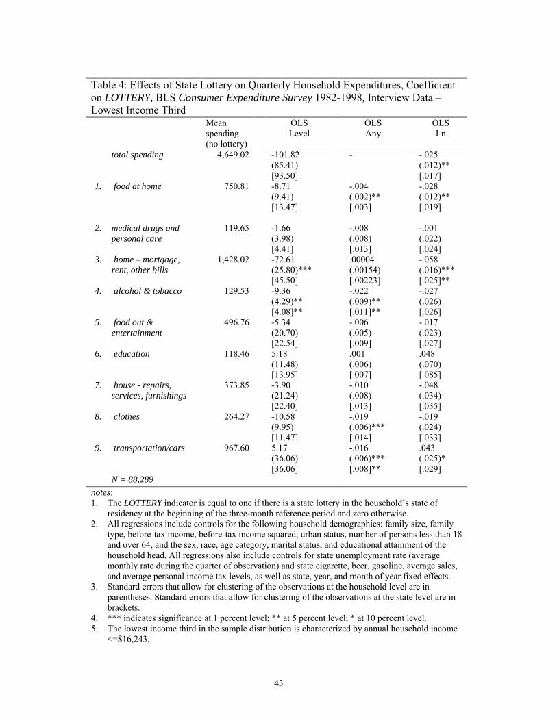
43
Table 4: Effects of State Lottery on Quarterly Household Expenditures, Coefficient on LOTTERY, BLS Consumer Expenditure Survey 1982-1998, Interview Data – Lowest Income Third Mean
spending (no lottery)
OLS Level
OLS Any
OLS Ln
total spending 4,649.02 -101.82 (85.41) [93.50]
- -.025 (.012)** [.017]
1. food at home 750.81 -8.71 (9.41) [13.47]
-.004 (.002)** [.003]
-.028 (.012)** [.019]
2. medical drugs and personal care
119.65 -1.66 (3.98) [4.41]
-.008 (.008) [.013]
-.001 (.022) [.024]
3. home – mortgage, rent, other bills
1,428.02 -72.61 (25.80)*** [45.50]
.00004 (.00154) [.00223]
-.058 (.016)*** [.025]**
4. alcohol & tobacco 129.53 -9.36 (4.29)** [4.08]**
-.022 (.009)** [.011]**
-.027 (.026) [.026]
5. food out & entertainment
496.76 -5.34 (20.70) [22.54]
-.006 (.005) [.009]
-.017 (.023) [.027]
6. education 118.46 5.18 (11.48) [13.95]
.001 (.006) [.007]
.048 (.070) [.085]
7. house - repairs, services, furnishings
373.85 -3.90 (21.24) [22.40]
-.010 (.008) [.013]
-.048 (.034) [.035]
8. clothes 264.27 -10.58 (9.95) [11.47]
-.019 (.006)*** [.014]
-.019 (.024) [.033]
9. transportation/cars
967.60 5.17 (36.06) [36.06]
-.016 (.006)*** [.008]**
.043 (.025)* [.029]
N = 88,289 notes: 1. The LOTTERY indicator is equal to one if there is a state lottery in the household’s state of
residency at the beginning of the three-month reference period and zero otherwise. 2. All regressions include controls for the following household demographics: family size, family
type, before-tax income, before-tax income squared, urban status, number of persons less than 18 and over 64, and the sex, race, age category, marital status, and educational attainment of the household head. All regressions also include controls for state unemployment rate (average monthly rate during the quarter of observation) and state cigarette, beer, gasoline, average sales, and average personal income tax levels, as well as state, year, and month of year fixed effects.
3. Standard errors that allow for clustering of the observations at the household level are in parentheses. Standard errors that allow for clustering of the observations at the state level are in brackets.
4. *** indicates significance at 1 percent level; ** at 5 percent level; * at 10 percent level. 5. The lowest income third in the sample distribution is characterized by annual household income
<=$16,243.

44
Table 5: Effects of State Lottery with Instant Games on Quarterly Household Expenditures, BLS Consumer Expenditure Survey 1982-1998, Interview Data OLS Level OLS Ln (1) (2) (3) (4) Full Sample
Lottery - 13.90 (109.21) [77.90]
- -.006 (.010) [.010]
Lottery with Instant -171.02 (55.52)*** [79.29]**
-182.19 (108.74)* [81.72]**
-.026 (.006)*** [.012]**
-.022 (.010)** [.012]*
Lowest income Lottery - 71.66
(192.53) [97.89]
- .007 (.022) [.016]
Lottery with Instant -143.25 (87.16)* [85.72]**
-203.27 (194.72) [100.38]**
-.031 (.011)*** [.016]**
-.037 (.022)* [.017]**
Middle income Lottery - -29.73
(120.76) [84.63]
- .003 (.014) [.013]
Lottery with Instant -51.92 (66.14) [71.18]
-27.89 (117.28) [78.81]
-.016 (.008)** [.012]
-.019 (.014) [.013]
Highest income Lottery - 92.50
(204.19) [124.52]
- -.002 (.013) [.008]
Lottery with Instant -260.28 (114.09)** [124.25]**
-331.55 (202.63) [132.44]
-.021 (.008)*** [.010]**
-.019 (.013) [.008]
notes: 1. The LOTTERY variable equals one if there is a state lottery in the household’s state of
residency at the beginning of the three-month reference period and zero otherwise. The PLUS_INSTANT indicator variable records whether the state lottery sells instant tickets.
2. All regressions include controls for the following household demographics: family size, family type, before-tax income, before-tax income squared, urban status, number of persons less than 18 and over 64, and the sex, race, age category, marital status, and educational attainment of the household head. All regressions also include controls for state unemployment rate (average monthly rate during the quarter of observation) and state cigarette, beer, gasoline, average sales, and average personal income tax levels, as well as state, year, and month of year fixed effects.
3. Standard errors that allow for clustering of the observations at the household level are in parentheses. Standard errors that allow for clustering of the observations at the state level are in brackets.
4. *** indicates significance at 1 percent level; ** at 5 percent level; * at 10 percent level. 5. The lowest income third in the sample distribution is characterized by annual household
income <=$16,243; the highest is >=$45,506.

45
Table 6: Effects of a State Lottery on Gambling Participation, Difference-in-Difference Estimates Dep Variable Mean of
“any” (no lottery)
any lottery track bingo private unlicensed
Overall (n=2,572)
.585
.072 (.051)
.429*** (.036)
.011 (.027)
-.002 (.027)
.009 (.034)
-.023 (.033)
Lowest income (n=629)
.461 .231*** (.092)
.448*** (.072)
-.008 (.045)
-.003 (.053)
.057 (.071)
-.031 (.056)
Middle income (n=991)
.682 .063 (.080)
.469*** (.063)
.053 (.043)
.064 (.045)
.065 (.054)
.002 (.055)
Highest income (n=952)
.723 -.001 (.065)
.392*** (.066)
-.001 (.059)
-.091 (.052)
-.056 (.060)
-.049 (.066)
notes: 1. Data on participation in the five types of gambling are from the 1975 National Survey of Adult Gambling conducted by Kallick et al. at the University of Michigan and the 1998 National Survey on Gambling conducted by the National Opinion Research Council (NORC) under contract with the National Gambling Impact Study Commission. The Kallick et. al. [1975) data consist of 1,749 completed interviews covering participants’ lifetime and past-year gambling behavior. The NORC [1998) data contain information about the gambling behavior of 2,417 adults from a random-digit dial sample. “Any” gambling is not equal to the sum of the five types of gambling displayed because the 1998 file separately categorizes participation in casino, charitable, card, bar/restaurant, internet, and indian reservation gambling. 2. The reported difference-in-difference estimate is the coefficient on LOTST7597*year1997 — the interaction between an indicator variable for the year 1997 and an indicator variable for residing in a state that adopted a lottery between 1975 and 1997. 3. All regressions control for sex, race, marital status, education, and regular attendance at religious services. They also control for main year and state effects. 4. Standard errors are White’s robust standard errors adjusted for clustering within a state-year cell. 5. *** indicates significance at 99 percentile ** at 95 percentile

46
Table 7: Weekly Ln Lotto Sales per Adult as a Function of Game Attributes dep var: ln(pasales)
(1) (2) (3) (4) (5)
Expected value -.773
(.560) .739
(.282) *** .882
(.219) *** .515
(.105) *** .505
(.103) ***
Variance/1M. .057 (.013)
*** .017 (.010)
* -.016 (.016)
.009 (.002)
*** .005 (.002)
**
skewness /1T -.0002 (.00006)
*** -.000009 (.00006)
.00006 (.00007)
-.00004 (.000007)
*** -.00002 (.000008)
**
nominal top prize/1M.
- - .011 (.007)
- .003 (.0008)
***
no. draws per week - -.014 (.043)
-.003 (.045)
- -
age of game - -.073 (.073)
-.057 (.074)
-.107 (.096)
-.108 (.097)
(age of game)2 - .021 (.005)
*** .021 (.005)
*** .023 (.005)
*** .023 (.005)
***
pick 5 - .576 (.276)
** .505 (.289)
* - -
pick 6 - .278 (.235)
.271 (.231)
- -
pick 7 - 1.01 (.246)
*** .982 (.225)
*** - -
cash jackpot - -1.16 (.325)
*** -1.14 (.310)
*** - -
choice (cash/ann) - .450 (.336)
.364 (.284)
- -
state unemployment rate
-.033 (.032)
-.028 (.029)
-.030 (.029)
-.038 (.019)
** -.038 (.019)
**
product fixed effects
no no no yes yes
state fixed effects yes yes yes yes yes week fixed effects yes yes yes yes yes demog. controls* yes yes yes yes yes constant -249.1
(220.2) -3.21
(122.8) -26.51
(123.4) 58.48
(253.4) 57.75
(253.4)
sample size 14,711
13,972 13,972 14,711 14,711
R2 .60 .87 .87 .91 .91 notes: 1. Unit of observation is state-week-game. 2. The sample includes 91 lotto products from 33 states. 3. Standard errors are adjusted for clustering at the state level, to flexibly account for correlation among the residuals. 4. Lottery sales data are from Lefleurs inc. 5. Data on game characteristics is compiled by author using information provided by state lottery associations. 6. Monthly state unemployment data are from the Bureau of Labor Statistics. 7. All regressions are population weighted. All regressions control for the proportion of the state population in the following categories: females age 18-24, 25-44, 45-64, 64+, males age 18-24, 25-44, 65+. Yearly state population figures are from the U.S. Census Bureau.

47
Appendix Table 1: Implementation dates State
lottery Instant games
State lottery
Instant games
Northeast
New England Middle Atlantic Connecticut 2/72 9/95 New Jersey 12/70 6/75 Maine 6/74 1/75 New York 6/67 1/76 Massachusetts 3/72 5/74 Pennsylvania 3/72 5/75 New Hampshire 3/64 5/96 Rhode Island 5/74 5/76 Vermont 2/78 6/78
Midwest East North Central West North Central Illinois 6/74 10/75 Iowa 8/85 8/85 Indiana 10/89 10/89 Kansas 11/87 11/87 Michigan 11/72 10/75 Minnesota 4/90 4/90 Ohio 8/74 6/76 Missouri 1/86 1/86 Wisconsin 9/88 9/88 Nebraska 9/93 9/93 North Dakota - - South Dakota 9/87 9/87
South South Atlantic South Central Delaware 10/75 2/76 Alabama - - District of
Columbia 8/82 8/82 Arkansas - -
Florida 1/88 1/88 Kentucky 4/89 4/89 Georgia 6/93 6/93 Louisiana 9/91 9/91 Maryland 5/73 2/76 Mississippi - - North Carolina - - Oklahoma - - South Carolina* 1/02 1/02 Tennessee* 1/04 1/04 Virginia 9/88 9/88 Texas 5/92 5/92 West Virginia 1/86 6/86
West Mountain Pacific Arizona 7/81 7/81 Alaska - - Colorado 1/83 10/84 California 10/85 2/90 Idaho 7/89 7/89 Hawaii - - New Mexico 4/96 4/96 Oregon 4/85 4/85 Nevada - - Washington 11/82 11/82 Montana 6/87 6/87 Utah - - Wyoming - - note: South Carolina and Tennessee implemented lotteries after the analysis period.

48
Appendix Table 2: Lottery Sales (in Year 2000 Dollars) Mean state sales All states Monthly total
(in millions) Monthly per adult sales
Yearly total (in millions)
No. of states (inc. DC) with
lotteries
No. of states reporting
sales Overall 78.8 18.3 33,409 - - 1992 67.8 16.0 24,207 35 32 1993 80.8 17.5 31,574 37 34 1994 86.3 18.9 34,158 37 33 1995 78.1 18.9 34,671 37 37 1996 81.0 18.5 34,981 38 36 1997 78.7 18.3 34,951 38 37 1998 77.1 18.9 34,287 38 38 notes: 1. Lottery sales data is from Lefleurs inc., who collects information from state lottery agencies. 2. Population figures used for per adult calculations are BLS census population numbers. 3. These figures reflect sales on all lottery games, including lotto, multi-state lotto, numbers, instant, keno, sports, bingo, and VLT products.
Top Related