


Languages
Pages
Legal


Specification of Landmarksand Forecasting Water Temperature
–Water Management in the River Wupper
Goran KauermannCenter for StatisticsUniversity Bielefeld
Thomas MestekemperUniversity Bielefeld
14. August 2008

The River Wupper
14. August 2008 1
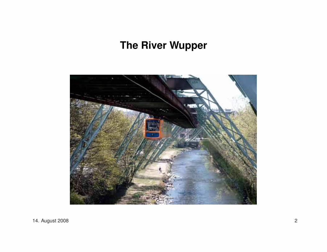
The River Wupper
14. August 2008 2

The River Wupper and its Power Plants
14. August 2008 3

The EU Water Framework Directive
Commits European Union member states to achieve good qualitativeand quantitative status of water bodies until 2015.
Good surface water status means both, good ecological and chemicalstatus. The first refers to the quality and functioning of the aquatic eco-system.
For the Wupper this implies:
Reduce electric power production“Too warm upstream water” =⇒or even shut down power plant
Definition of “Warm Water” depends on the fish life and reproductioncycle and the given threshold may vary over the year.
14. August 2008 4

Outline of Talk
• Forecasting (upstream) Water Temperature
• Specification of Landmarks (Threshold, dependent fish spawning cycle)
• Discussion
14. August 2008 5

Literature on Water Temperature Forecasting
Hydrological Literature:
• Seasonal and daily variations of water temperature are significantlyimportant for aquatic resources. (Caissie et al., 2005, Hydrological Proces-ses)
• Two model classes: physical (thermo-dynamic) and stochastic (stati-stical) models. (Webb et al., 2008, Hydrological Processes)
Statistical Literature:
• Functional component models or dynamic factor models. (Cornillon etal., 2008, CSDA; Stock & Watson, 2006, Handbook of Economic Forecasting)
• Functional Time Series. (Ferraty & Vieu, 2006, Nonparametric FDA, Springer-Verlag)
14. August 2008 6

Smooth Cyclic Estimation
Let index t = (y, d) denote time with year y, day in year d and wt andat be a 24-dimensional vectors of the hourly water and air temperature,respectively, which decompose to
wt = µw(d) + wt, at = µa(d) + ayd.↑ ↑
yearly trend yearly trend
Functions µw(d) and µa(d) are fitted with “wrapped” B-splines, i. e.
limd→365+
µw(d) = limd→1−
µw(d).
14. August 2008 7

Average Temperatures µw and µa
14. August 2008 8

Functional Principal Components Decomposition
wt shall be decomposed to a dynamic factor model, that is, we reducedimensions by extracting k suitable factors (done by PCA):
wt = ftΛTw + εw,t
where Λw is a 24 × k dimensional loading matrix, ft a k dimensionalfactor and εw,t a white noise residual.
Accordingly for the air temperature we extract h suitable factors:
at = gtΛTa + εa,t
14. August 2008 9

Fitted Principal Components
5 10 15 20
−0.
2−
0.1
0.0
0.1
0.2
0.3
water temperature
hour
fact
or lo
adin
g
1
2
5 10 15 20
−0.
3−
0.2
−0.
10.
00.
10.
2
air temperature
hourfa
ctor
load
ing
1
2
14. August 2008 10

The Dynamic Factor ModelUsing the backshift operator ∆a,bft = (ft−a, . . . , ft−b). We assume anautoregressive model for the factor ft:
ft = (∆1,pft)βf + (∆0,qgt)βg + εf,t.
This implies that ft depends on:
• water temperature factors of the p previous days
• air temperature factors of the q previous days
• the current day air temperature factors.
Note: In a forecasting setting the last point is only available asmeteorological forecast.
14. August 2008 11

Estimation of the factors ft and gt
We want to compare three different approaches to estimate the factors.
1) We start with a quite simple Least Squares estimation method wherethe facor loadins are taken as
ft = wtΛw and gt = atΛa
Pro: The remaining parameters βf and βgcan easily be foundusing least squares regression.
Con: The resulting estimates are not Maximum Likelihood-based.
We need to incorporate our stochastic models in the estimation method.
14. August 2008 12

Estimation of the factors ft and gt (continued)
2) In a Maximum Likelihood approach we assume that the residuals inthe former mentioned models follow normal distributions:
εw,t ∼ N(0, diag(σ2
w))
and εf,t ∼ N(0, diag(σ2
f)).
3) We incorporate a stochastic autoregressive model for the air tempe-rature, as well, in a Full Maximum Likelihood estimation method:
gt = (∆1,qgt)βg + εg,t
asuming εa,t ∼ N(0, diag(σ2
a))
and εg,t ∼ N(0, diag(σ2
g)).
The unknown parameters θ = (βf , βg, σ2f , σ2
w) and θ = (θ, βg, σ2g, σ
2a)
are now estimated using an EM-algorithm.
14. August 2008 13

Model Selection (in progress)In order to select the best performig model we divide our dataset in atraining and a forecasting sample. To measure the model quality onecould, for example, make use of the Mean Squared Prediction Errordefined by:
MSPE =1n
n∑
t=i
(wt − wt)(wt − wt)T .
We have to select:
• k and h; the optimal number of factors for water and air temperature,respectively,
• p and q; the optimal number of time lags for water and air tempera-ture, respectively, (we treat q = 2 as fixed)
• the optimal estimation method.
14. August 2008 14

DemonstrationWarm spring days over Whitsun 2008
5 10 15 20
1314
1516
17
Temperature
Hou
r
10.5.200811.5.12.5.13.5.14.5.15.5
14. August 2008 15

Demonstration
0 10 20 30 40 50 60 70
1213
1415
16
Hour
Tem
pera
ture
Real vs. Forecasted Temperature
realforecasted
5 10 15 20
0.20
0.25
0.30
0.35
0.40
HourR
MS
E
Root Mean Square Error
14. August 2008 16

Multiple Day Forecast
Multiple day forecasts show discontinuities.
Solution: To achieve a continuous m day forecast we divide our timeaxis into time intervals of length m, i. e.
wmt = wt = (wyd1, . . . ,wyd24,wy(d+1)1, . . .wy(d+m)24)
The above models are re-fitted in analogy to the 24h case.
14. August 2008 17

Demonstration
0 10 20 30 40 50 60 70
1213
1415
16
Hour
Tem
pera
ture
Real vs. forecasted Temperature
realforecasted
0 10 20 30 40 50 60 70
0.2
0.3
0.4
0.5
0.6
HourR
MS
E
Root Mean Square Error
14. August 2008 18

Comparison to other modelling approaches
We compared our Least Squares model to three approaches to modelthe daily maximum temperature presented in Cassie et al. (1998, Can. J. Civ.Eng.)
1. wmaxt = (∆0,2a
maxt )β1 + ε1t resulted in an RMSE of 1.295◦C.
2. wmaxt = (∆1,2w
maxt )β2 + K amax
t resulted in an RMSE of 2.439◦C.
3. wmaxt = ζ0
1−δ1B amaxt + 1
1−φ1Bnt resulted in an RMSE of 1.018◦C.
For p = 2, q = 1, k = h = 3 and q = 2 our Least Squares Model yieldedan RMSE of 0.42◦C.
14. August 2008 19

Finding Seasonal Pattern
Besides forecasting is the specification of seasonal pattern an importantissue, since:
• Water temperature has to stay below ecologically justified thresholdsto preserve the fish populations.
• Threshold values depend on season, or more precisely on reproduc-tion cycle of fish.
• Seasons can vary like an early spring or late summer.
• What is the “reference year”?
14. August 2008 20

Literature in ’Warping’ and ’Landmark Specification’
• Landmark specification in growth curves. (Kneip & Gasser, 1992, Annalsof Statistics; Gasser & Kneip, 1995, JASA)
• Automatic Warping (or self-modelling). (Ramsay & Li, 1998, JRSS B; Ger-vini & Gasser, 2004, JRSS B)
• We need an “online” warping, as data arrives over time.
14. August 2008 21

Structure of Water temperature
time (months)
tem
pera
ture
(C
elsi
us)
7 8 9 10 11 12 1 2 3 4 5 6
010
2030
4050
60
20012002
20022003
20032004
20042005
20052006
20062007
temperature curves
14. August 2008 22

Different modelling for landmark registration
Let t = (y, d, h) where h is the hour in day d.
water: wt = wydh = wyd + xydh
↑ ↑daily avg. temp. residual
↓ ↓air: at = aydh = ayd + zydh
A principal component analysis is run on the residuals xydh and zydh
after substracting the mean daily temperature course:
xydh = µx(d) + xydh and zydh = µz(d) + zydh.
14. August 2008 23

Seasonal Pattern in PCA coefficients
xydh = µx(h) +Kx∑
k=1
fyd,kλx,k(h)
5 10 15 20
−0.
40.
00.
20.
4
12
3
1
2
3
principal components
2002 2003 2004 2005 2006 2007
−10
−5
05
first score
2002 2003 2004 2005 2006 2007
−4
−2
01
2
second score
2002 2003 2004 2005 2006 2007
−2
02
4
third score
14. August 2008 24

Landmark based on First PCA Score
We check, whether H0 : E(fyd,1) ≤ 0 is rejected.
time
scor
e
−10
−5
05
10
2002 2003 2004 2005 2006 2007
253 95 267 80 283 90 236 93 237 123 279 96
first principal component scores
time
p−va
lue
0.05
0.95
2002 2003 2004 2005 2006 2007
253 95 267 80 283 90 236 93 237 123 279 96
p−value taking into account 15 consecutive days
time
tem
pera
ture
510
1520
2002 2003 2004 2005 2006 2007
253 95 267 80 283 90 236 93 237 123 279 96
average daily temperature
14. August 2008 25

Correlation between Water and Air Temperature
Water: xydh = µx(h) +K∑
k=1
fyd,kλx,k(h)
Air: zydh = µz(h) +K∑
k=1
gyd,kλz,k(h)
Canonical correlation:For coefficient vectors δT
k and γTk we obtain the maximal correlation bet-
ween water and air temperature, i. e.
max Cor(δTk xt, γ
Tk zt), k = 1, 2, . . .
14. August 2008 26

Canonical Correlation Landmark
5 10 15 20
−0.
6−
0.2
0.2
daytime
cano
nica
l com
pone
nt 1
23
123
canonical component water temperature
5 10 15 20
−1
01
2
daytime
cano
nica
l com
pone
nt
123
123
canonical component air temperature
14. August 2008 27

Canonical Correlation ContributionsWe look at the canonical correlation:
water: ωt = δT1 xt air: νt = γT
1 zt both: ωt · νt
−0.06 −0.04 −0.02 0.00 0.02 0.04 0.06
−0.
08−
0.04
0.00
0.04
water temperature
air
tem
pera
ture
canonical correlation scores
2003 2004 2005 2006 2007
−2
02
46
8
time (year)
corr
elat
ion
contribution to first canonical correlation
81 87 92 123 92229 248 211 215 206
14. August 2008 28
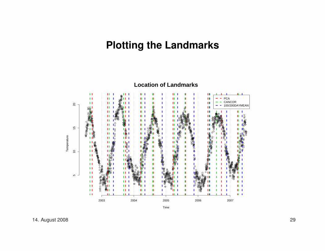
Plotting the Landmarks
Time
Tem
pera
ture
Location of Landmarks
510
1520
2003 2004 2005 2006 2007
PCACANCOR100/200DAYMEAN
14. August 2008 29

Warping the Years
Standard Time
Rea
l Tim
e
late
early
Time Warping Functions
02/0303/0404/0505/0606/07
J A S O N D J F M A M J
JA
SO
ND
JF
MA
MJ
14. August 2008 30

Discussion
• Analysis on Forecasting of Water Temperature is an important issue(and is getting even more important based on new EU laws).
• The issue is not fully covered by classical and newer approaches intime series analysis.
• Finding landmarks for seasonal variation is relevant from an ecologi-cal point of view.
• More to do: Compare our time warp results to observed fish spawningcycles.
14. August 2008 31
Top Related