


Languages
Pages
Legal


Spatial Regression: The Curious Case ofNegative Spatial Dependence
Sheena Yu-Hsien Kao∗and Anil K. Bera†
April 9, 2016
1 Introduction
Positive spatial dependence is predominant in the spatial data. Therefore, it is
not surprising that most of the methodological papers are concerned with the
positive spatial dependence (either in terms of spatial lag, spatial error, or both)
when evaluating estimation, testing and forecasting procedures [For example,
see Anselin, Bera, Florax, and Yoon (1996) and Baltagi, Song, and Koh (2003)
for testing spatial dependence.] However, prevalence of negative spatial depen-
dence is not uncommon as evidenced in many applied papers; just to mention
a few: the studies of welfare competition or federal grants competition among
local governments [Saavedra (2000) and Boarnet and Glazer (2002)]; regional
employment [Filiztekin (2009) and Pavlyuk (2011)]; the cross-border lottery
shopping [Garrett and Marsh (2002)]; foreign direct investment [Garretsen and
Peeters (2009); Blanc-Brude, Cookson, Piesse and Strange (2014); Nwaogu and
Ryan (2014)]; land use changes [He, Huang and Wang (2014)]; growth spillover
through trade [Behrens, Ertur and Kock (2013); Ho, Wang and Yu (2014)]
and locations of Turkish manufacturing industry [Basdas (2009)]. Griffith and
Arbia (2010) investigated empirical situations in which negative spatial depen-
dence may occur and situations in which it may be masked by positive spatial
autocorrelation. In particular, they presented examples of negatively spatial au-
tocorrelated phenomena based on the geographic competition for land surface,
∗Department of Economics, University of Illinois. E-mail: [email protected]†Department of Economics, University of Illinois. E-mail: [email protected]
1

for territory, and for market area.
The literature of theoretic explanation for the presence of negative spatial
dependence is still growing slowly. Some attempts have been made in economic
theory recently, especially in trade and growth theory. For example, Frank
and Botolf (2007) suggest that Myrdal’s backwash effect [Myrdal (1957)] can be
used to explain the empirical finding of negative spatial autocorrelation in the
German regional information and computer technology (ICT) distribution. The
backwash effect discussed in Myrdal (1957) implies that growth in one region
is harmful for growth in neighbor regions since it may attract resources and
skilled labor from neighbor regions and reduce their growth potential. Blonigen,
Davies, Waddell, and Naughton (2004) discussed theoretical models for different
kinds of Foreign Direct Investment (FDI) and their theory predicts negative
spatial dependence for pure vertical FDI and export platform FDI because the
production set-up from home country to host country is directly at the cost of
other host countries. It appears that negative spatial autocorrelation is likely
to occur when competition between regions (or agents) outweigh cooperative
factors.
In contrast to the time-series analysis, positive and negative spatial depen-
dence can have quite different implications. Consider a simple first-order au-
toregressive model,
yt = ρyt−1 + εt, |ρ| < 1, t = 1, 2, ..., T.
where εt ∼ IID(0, σ2ε ), and yt ∼ (0, σ2
ε ). The variance-covariance matrix of y has
the diagonal elements equal to σ2ε/(1−ρ2) and off-diagonal ones Vij = σ2
1−ρ2ρ|i−j|.
Therefore, the only difference between positive or negative autocorrelation is
just the sign of the elements in the matrix. Thus, theoretically there is not much
difference between positive or negative autocorrelation in terms of properties of
the model. Moreover, previous Monte Carlo studies such as Kramer and Zeisel
(1990), King (1985), L’Esperance and Taylor (1975), and Park (1975) suggest
that the empirical power functions of various tests for serial autocorrelation, for
example Durbin-Watson test and BLUS test, appear to be symmetric around
zero and the symmetry becomes more apparent when the sample size (T ) grows.
2
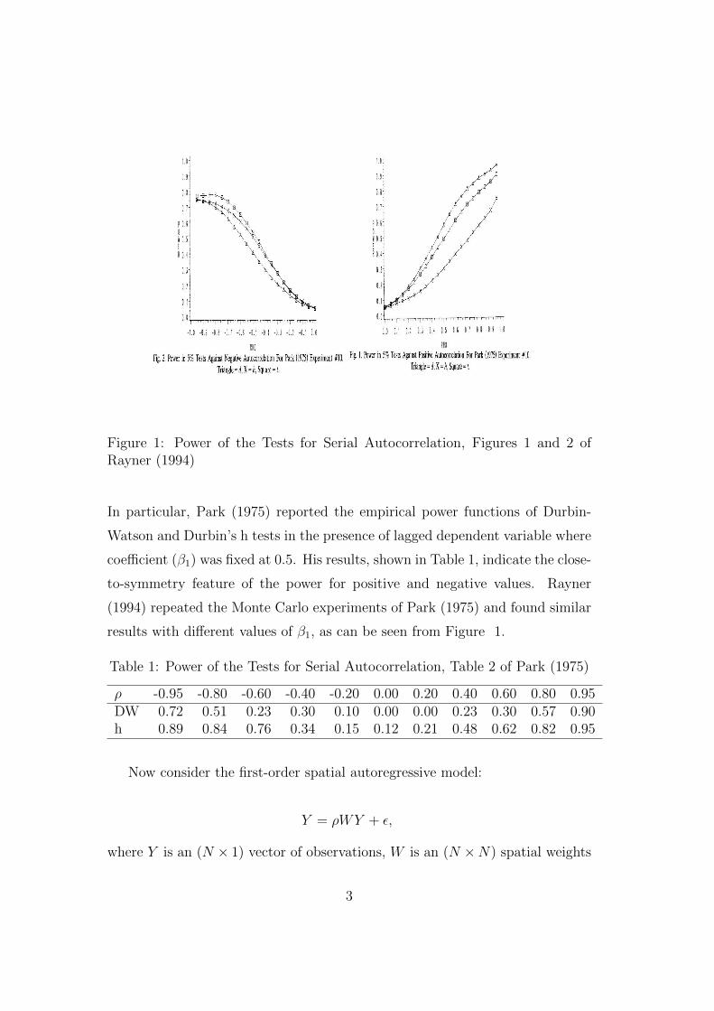
Figure 1: Power of the Tests for Serial Autocorrelation, Figures 1 and 2 ofRayner (1994)
In particular, Park (1975) reported the empirical power functions of Durbin-
Watson and Durbin’s h tests in the presence of lagged dependent variable where
coefficient (β1) was fixed at 0.5. His results, shown in Table 1, indicate the close-
to-symmetry feature of the power for positive and negative values. Rayner
(1994) repeated the Monte Carlo experiments of Park (1975) and found similar
results with different values of β1, as can be seen from Figure 1.
Table 1: Power of the Tests for Serial Autocorrelation, Table 2 of Park (1975)
ρ -0.95 -0.80 -0.60 -0.40 -0.20 0.00 0.20 0.40 0.60 0.80 0.95DW 0.72 0.51 0.23 0.30 0.10 0.00 0.00 0.23 0.30 0.57 0.90h 0.89 0.84 0.76 0.34 0.15 0.12 0.21 0.48 0.62 0.82 0.95
Now consider the first-order spatial autoregressive model:
Y = ρWY + ε,
where Y is an (N × 1) vector of observations, W is an (N ×N) spatial weights
3

matrix and ε ∼ (0, Iσ2ε ). The variance-covariance matrix of Y can be written as,
V ar(Y ) = (I − ρW )−1((I − ρW )′)−1σ2ε .
Because of the feature of W , the structures of the above matrix for positive
or negative values of ρ can be very different. For example, when n = 6, σ2ε = 1,
and W based on a 3×2 regular grid with queen criterion, the variance-covariance
matrix of Y for ρ = 0.5 and ρ = −0.5 are respectively.
V ar(Y ) =
1.406 0.602 0.319 0.671 0.602 0.319
0.602 1.431 0.602 0.602 0.605 0.602
0.319 0.602 1.406 0.319 0.602 0.671
0.671 0.602 0.319 1.406 0.602 0.319
0.602 0.605 0.602 0.602 1.431 0.602
0.319 0.602 0.671 0.319 0.602 1.406
,
V ar(Y ) =
1.174 -0.230 0.087 -0.266 -0.230 0.087
-0.230 1.162 -0.230 -0.230 -0.072 -0.230
0.087 -0.230 1.174 0.087 -0.230 -0.266
-0.266 -0.230 0.087 1.174 -0.230 0.087
-0.230 -0.072 -0.230 -0.230 1.162 -0.230
0.087 -0.230 -0.266 0.087 -0.230 1.174
.
Comparing the two matrices, both in terms of signs and magnitudes of the el-
ements, it is hard to detect any particular pattern. This is one of the motivating
factors to study other properties with negative value of spatial autocorrelation.
Previous studies on testing spatial models usually concentrated only on pos-
itive spatial dependence. Anselin and Rey (1991), however, considered both
positive and negative values in their Monte Carlo studies to compare the prop-
erties of Moran’s I and Rao’s score (RS) tests, separately for spatial error and
spatial lagged dependence, and their results are shown in Figure 2. Though
not symmetric around zero, we notice that the power of both tests increase as
the true value of spatial autocorrelation coefficient move away from zero. As
expected, asymmetry of the tests is more prominent for smaller sample sizes.
Anselin, Bera, Florax and Yoon (1996) considered the joint presence of lag and
4

(a) Power of Moran’s I
(b) Power of Rao score Test
Figure 2: Empirical Power Functions in Anselin and Rey (1991)
error dependence; however, negative parameter values were excluded in their
simulation study.
This paper is concerned with the case of negative spatial dependence and
its consequence on specification tests and calculation of impact effects. We
will investigate how negative spatial dependence has bearings upon econometric
analysis and in particular, first we will extend the theory and Monte Carlo
results in the literature by including negative coefficients. We will also extend
the theoretical derivation and simulations to compare various tests for spatial
autocorrelation in Anselin et al. (1996). Then we will specifically show how we
need to alter the standard methodologies for model specification and evaluation
5
in the presence of negative spatial dependence.
2 A General Approach to testing in the presence of a nuisance pa-rameter
Consider a general statistical model represented by the log-likelihood function
L(γ, ψ, φ), where γ is a parameter vector, and for simplicity ψ and φ are taken
as scalars to conform with the spatial autoregressive model. Suppose an in-
vestigator sets φ = 0 and tests H0 : ψ = ψ0 using the log-likelihood function
L1(γ, ψ) = L(γ, ψ, φ0), where ψ0 and φ0 are known values. The RS test statis-
tic for testing H0 under L1(γ, ψ) will be denoted by RSψ. Let us also denote
θ = (γ′, ψ′, φ′)′ and θ = (γ′, ψ′0, φ′0), where γ is the maximum likelihood estima-
tor (MLE) of γ when ψ = ψ0 and φ = φ0. The score vector and the information
matrix are defined, respectively, as
d(θ) =∂L(θ)
∂θ=
∂L(θ)∂γ
∂L(θ)∂ψ
∂L(θ)∂φ
and
J(θ) = −E[
1
N
∂2L(θ)
∂θ∂θ′
]=
Jγ Jγψ Jγφ
Jψγ Jψ Jψφ
Jφγ Jφψ Jφ
.If L1(γ, ψ) were the true model, it is well known that under H0 : ψ = ψ0,
RSψ =1
Ndψ(θ)′J−1
ψ�γ(θ)dψ(θ)D→ χ2
1(0),
where Jψ�γ = Jψ(θ)− JψγJ−1γ Jγψ. We use
D→ to denote convergence in distribu-
tion. Under H1 : ψ = ψ0 + ξ/√N ,
RSψD→ χ2
1(λ1), (1)
where the noncentral parameter λ1 = ξ′Jψ�γξ. Under the set-up, asymptotically
the test will have the correct size and will be locally optimal. Now suppose
that the true log-likelihood function is L2(γ, φ) = L(γ, ψ0, φ), so the alternative
6

L1(γ, ψ) becomes completely misspecified. Using a sequence of local values φ =
φ0 + δ/√N , Davidson and MacKinnon (1987) and Saikkonen (1989) obtained
the asymptotic distribution of RSψ under L2(γ, φ) as
RSψD→ χ2
1(λ2), (2)
where λ2 = δ′Jφψ�γJ−1ψ�γJψφ�γδ, with Jψφ�γ = Jψφ − JψγJ−1
γ Jγφ.
Turning to the case of undermisspecification, let the true model be repre-
sented by the log-likelihood L(γ, ψ, φ). The alternative L1(γ, ψ) is underspeci-
fied with respect to nuisance parameter φ, leading to the problem of undertest-
ing. Consider the local departure φ = φ0+δ/√N together with ψ = ψ0+ξ/
√N .
For this case Bera and Yoon (1991) derived the asymptotic distribution of RSψ,
RSψD→ χ2
1(λ3), (3)
where
λ3 = (δ′Jφψ�γ + ξ′Jψ�γ)J−1ψ�γ(Jψφ�γδ + Jψ�γξ)
= λ1 + λ2 + 2ξ′Jψφ�γδ.
Using the result, we can compare the asymptotic local power of the under-
specified test with that of the optimal test. It turns out that the contaminated
non central parameter λ may increase or decrease the power depending on the
configuration of the term ξ′Jψφ�γδ.
Utilizing (2), adjusting the mean and variance of RSψ, Bera and Yoon (1993)
suggested a modification so that resulting test is valid in the local presence of
φ. The modified statistic is given by
RS∗ψ =1
N[dψ(θ)− Jψφ�γ(θ)J−1
φ�γ(θ)dφ(θ)]′
×[Jψ�γ(θ)− Jψφ�γ(θ)J−1φ�γ(θ)Jφψ�γ(θ)]
−1
×[dψ(θ)− Jψφ�γ(θ)J−1φ�γ(θ)dφ(θ)].
(4)
Under ψ = ψ0 and φ = φ0 + δ/√N, RS∗ψ has a central χ2
1 distribution, and
under the local alternative ψ = ψ0 + ξ/√N ,
7

RS∗ψD→ χ2
1(λ4), (5)
where λ4 = ξ′(Jψ�γ − Jψφ�γJ−1φ�γJφψ�γ)ξ.
Similarly, we can also obtain RS∗φ to test H0 : φ = φ0 in the presence of
local misspecification and derive the noncentral parameters of RSφ and RS∗φ.
If L2(γ, φ) is the true log-likelihood function, under the null hypothesis RSφ
asymptotically follows central χ21 distribution, and under local alternative φ =
φ0 + δ/√N ,
RSφD→ χ2
1(λ5), (6)
where λ5 = δ′Jφ�γδ. In the case of complete misspecification, we have
RSφD→ χ2
1(λ6), (7)
where λ6 = ξ′Jψφ�γJ−1φ�γJφψ�γξ. And in the case of undermisspecification,
RSφD→ χ2
1(λ7), (8)
where λ7 = λ5 + λ6 + 2δ′Jφψ�γξ.
On the other hand, the adjusted RS test statistic for testing H0 : φ = φ0 will
follow a central χ21 distribution under the null hypothesis even in the presence of
locally misspecification of ψ. And under the local alternative φ = φ0 + δ/√N ,
RS∗φD→ χ2
1(λ8). (9)
where λ8 = δ′(Jφ�γ − Jφψ�γJ−1ψ�γJψφ�γ)δ.
3 Tests for SARMA Model
To make the study comparable to previous literature on spatial analyses, we
consider a general model, the mixed regressive spatial autoregressive moving
average (SARMA) model, as specified in Anselin et al. (1996):
8

y = Xγ + φWy + u,
u = ψWε+ ε,
ε ∼ N(0, σ2I),
(10)
where y is an (n × 1) vector of observations of dependent variable, X is an
(n× k) matrix of observations of exogenous variables, and γ is a (k× 1) vector
of parameters. φ and ψ are scalar spatial parameters, and W is a (n×n) spatial
weights matrix.
We are interested in testing H0 : ψ = 0 in the presence of the nuisance
parameter φ. Let θ = (γ′, ψ, φ)′, following the result of Anselin (1988a), we
have the following equations:
∂L
∂γ= dγ =
1
σ2X ′u,
∂L
∂ψ= dψ =
1
σ2u′Wu,
∂L
∂φ= dφ =
1
σ2u′Wy,
(11)
and
J =
X ′X 0 X ′(WXγ)
0 ωσ2 ωσ2
(WXγ)′X ωσ2 (WXγ)′(WXγ) + ωσ2
, (12)
where ω = tr[(W ′ +W )W ]. Using (11) and (12), it is easy to show:
Jψφ�γ = Jψ�γ = Jφψ�γ =ω
n,
Jφ�γ =1
nσ2[(WXγ)′M(WXγ) + ωσ2]
=ω
n+
1
nσ2(WXγ)′M(WXγ),
(13)
where M = I −X(X ′X)−1X ′. The adjusted RS statistic can be constructed as,
RS∗ψ =[u′Wu/σ2 − ω(nJφ�γ)
−1u′Wy/σ2]2
ω[1− ω(nJφ�γ)−1], (14)
where u = y − Xγ are the OLS residuals, and σ2 = u′u/n, and from (13) it
follows that
9
(nJφ�γ)−1 = σ2[(WXγ)′M(WXγ) + ωσ2]−1.
The conventional one-directional test RSψ given in Burridge (1980) is ob-
tained by setting φ = 0 to yield
RSψ =[u′Wu/σ2]2
ω. (15)
To see the behavior of RSψ and RS∗ψ let us consider the case of local mis-
specification, i.e. φ = φ0 + δ/√n. Under the null ψ = 0 and alternative
ψ = ψ0 + ξ/√n, the noncentral parameters of RSψ are respectively
λ2 =ωδ2
n. (16)
and
λ3 = λ1 + λ2 + 2ξ′Jψφ�γδ
= ξ′(T
N)ξ + δ′(
T
N)δ + 2ξ′(
T
N)δ
=ω
n(ξ2 + δ2 + 2ξδ).
(17)
Therefore, the noncentral parameters of RSψ under both the null and al-
ternative are affected by δ, i.e., the local misspecification of φ. Comparing to
the case where both of the spatial autocorrelation parameters are positive, the
noncentral parameter is lower when they have opposite signs, and it can be as
low as 0 when ξ = −δ.On the other hand, the noncentral parameter of RS∗ψ under ψ = ψ0 + ξ/
√n
is not affected by the presence of local misspecification of φ, and is given by
λ4 = ξ′[ω
n− (
ω
n)2J−1
φ�γ]ξ
=ωξ2
n(1− ωσ2
ωσ2 + (WXγ)′M(WXγ)).
(18)
which depends, on ξ but free of δ, the local misspecification in φ.
In the presence of local misspecification, i.e. ψ = ψ0 + ξ/√n, we can also
study the performance of RS∗φ and RSφ, which are given by,
10

RS∗φ =[u′Wy/σ2 − u′Wu/σ2]2
nJφ�γ − ω(19)
and
RSφ =[u′Wy/σ2]2
nJφ�γ. (20)
Under the alternative φ = φ0 + δ/√N , the noncentral parameter of RS∗φ and
RSφ are respectively,
λ8 = δ′(1
nσ2)(WXγ)′M(WXγ)δ (21)
and
λ7 = δ′Jφ�γδ + ξ′Jψφ�γJ−1φ�γJφψ�γξ + 2δJφψ�γξ
= δ′(1
nσ2)[(WXγ)′M(WXγ) + ωσ2]δ
+ ξ′(ω2
n2)[(WXγ)′M(WXγ) + ωσ2]−1ξ + 2δ′(
ω
n)ξ
(22)
Again we observe that the noncentral parameter of RSφ is affected by the
combination of positive or negative values of δ and ξ, while that of RS∗φ is free
of this problem.
4 Empirical Applications
To gain more insights on how negative spatial dependence would affect model
specification tests and estimation in practice, we examine the various test statis-
tics and estimated parameters in the existing literature. Table 2 shows re-
sults from three common applications with positive spatial dependence. All of
them have the common features that (i) the unadjusted one-directional tests are
strongly significant and the joint tests are moderately significant, while the ad-
justed statistics are lower than the unadjusted ones and show less significance,
(ii) estimated spatial parameters are positive and significant. These examples
show that it is likely that both the unadjusted one-directional tests are spurious
because of only one source of spatial dependence.
11
On the other hand, the cases with negative spatial dependence are more
complicated. Table 3 summarizes some empirical results with negative spatial
coefficients. As indicated in the previous section, the unadjusted test statistics
can be higher or lower than the adjusted ones, depending on the combinations
of the signs of two sources of spatial dependence. For example, Garret and
Marsh (2002) estimated the revenue impact of cross-border lottery sales for 105
counties in Kansas and found negative spatial autocorrelation for both spatial
lag and spatial error coefficients. However, it should be noted that in their
study they estimated the two coefficients separately, not jointly. According to
the reported values of Rao-score test statistics and the theoretical prediction in
previous sections, we expect that both of the coefficients are negative.
Though there are many empirical studies that found negative spatial depen-
dence, most of the studies only estimate one spatial autocorrelation coefficient,
either spatial lag or spatial error, and reported one-directional Rao-score test
result. Others consider both two kinds of spatial dependence, but estimate
the coefficients separately, as we see in Garret and Marsh (2002), and Basdas
(2009). To further see the empirical applications of the interactions between
the two kinds of spatial dependence with negative values, it is necessary to rein-
vestigate the data that finds negative spatial autocorrelations. Therefore, we
illustrate the case of negative spatial dependence using the data of government
direct expenditure for the 48 U.S. continental states, based on the empirical
analyses of Case, Rosen, and Hines (1993) and Boarnet and Glazor (2001). In
their studies, the question of interest is the multiplying effect of federal grants
on state and local government expenditure, after controlling for the spatial de-
pendence. The studies use a panel data from 1970-1985; however, to focus on
the illustration of negative spatial dependence, we will only look at a cross sec-
tional data set. Therefore, the data we examine contains the state and local
government expenditure, grants received from federal government, and personal
income per capita in 2010.
Table 4presents the estimated spatial regression results which includes both
spatial dependence in lagged dependent variable and error. From the results we
see that the estimated spatial autocorrelation for lagged dependent variable (φ)
12

Table 2: Summary of Empirical Studies - Positive Dependence
RSψφ RSψ RS∗ψ RSφ RS∗
φ φ ψ
Anselin (1988) 9.44 5.72 0.08 9.36 3.72 0.431 0.562(<0.01) (0.02) (0.78) (<0.01) (0.05) (<0.01) (<0.01)
Florax (1992) 7.97 2.43 0.14 7.83 5.54 0.349 0.459(0.02) (0.12) (0.70) (0.02) (<0.01) (<0.01) (<0.01)
Anselin et al. (1996) 5.07 4.35 3.65 1.42 0.72 0.188 0.465(0.08) (0.04) (0.06) (0.23) (0.40) (0.11) (<0.01)
*p-values in parentheses.
Table 3: Summary of Empirical Studies - Negative Dependence
RSψφ RSψ RS∗ψ RSφ RS∗
φ φ ψ
Garret & Marsh (2002) 3.91 0.57 0.12 3.79 3.34 −0.064∗ −0.009∗
(0.14) (0.45) (0.73) (0.05) (0.07)Pavlyuk(2011) 7.37 0.03 5.00 2.37 7.34 −1.91∗
(0.03) (0.86) (0.03) (0.12) (<0.01)Basdas (2009) 6.26 3.77 5.43 0.83 2.49 −0.48∗
(0.04) (0.05) (0.02) (0.36) (0.11)
*Estimate coefficients separately.
is negative; while the estimated spatial autocorrelation for error (ψ) is positive.
The t statistics suggest that both spatial dependence are significant, and if we
ignore the spatial feature of the data and run OLS regression, there would be
an under estimation of the coefficient of federal grants, and the log-likelihood
of the model would decrease.
Furthermore, table 5shows the Rao-score statistics for model specification
tests of spatial dependence. The test statistics show how the negative values of
spatial autocorrelation would lead to a contradictory results of unadjusted one-
directional test with the joint test. From the test statistics, we can reject the
joint null hypothesis: H0 : φ = ψ = 0, but we cannot reject the one-directional
test of H0 : φ = 0 or H0 : ψ = 0 based on unadjusted test statistics. On the
other hand, the adjusted test statistics for both spatial dependence show that
the coefficients are significantly different from zero, consistent with the joint
test result and the t statistics in estimation result in table 5. The results are
similar with different specification of spatial weight matrices.
As addressed in Case et al. (1993) and Boarnet and Glazor (2001), the re-
search interest lies in measuring the multiplying effect of grants from federal on
state and local government expenditure, which requires a proper interpretation
of the estimated coefficient. In the standard linear regression, there is a straight-
forward interpretation of estimated coefficients; while in the spatial regression,
13
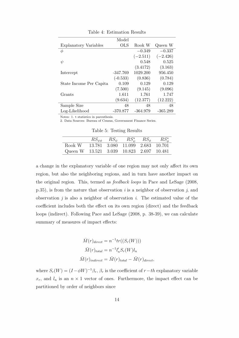
Table 4: Estimation Results
ModelExplanatory Variables OLS Rook W Queen W
φ −0.349 −0.337(−2.511) (−2.426)
ψ 0.548 0.525(3.4172) (3.163)
Intercept -347.769 1029.200 956.450(-0.533) (0.836) (0.784)
State Income Per Capita 0.109 0.129 0.129(7.500) (9.145) (9.096)
Grants 1.611 1.761 1.747(9.634) (12.377) (12.222)
Sample Size 48 48 48Log-Likelihood -370.877 -364.979 -365.289
Notes: 1. t statistics in parenthesis.2. Data Sources: Bureau of Census, Government Finance Series.
Table 5: Testing Results
RSψφ RSψ RS∗ψ RSφ RS∗φRook W 13.781 3.080 11.099 2.683 10.701Queen W 13.521 3.039 10.823 2.697 10.481
a change in the explanatory variable of one region may not only affect its own
region, but also the neighboring regions, and in turn have another impact on
the original region. This, termed as feedback loops in Pace and LeSage (2008,
p.35), is from the nature that observation i is a neighbor of observation j, and
observation j is also a neighbor of observation i. The estimated value of the
coefficient includes both the effect on its own region (direct) and the feedback
loops (indirect). Following Pace and LeSage (2008, p. 38-39), we can calculate
summary of measures of impact effects:
M(r)direct = n−1tr((Sr(W )))
M(r)total = n−1l′nSr(W )ln
M(r)indirect = M(r)total − M(r)direct,
where Sr(W ) = (I−φW )−1βr, βr is the coefficient of r−th explanatory variable
xr, and ln is an n × 1 vector of ones. Furthermore, the impact effect can be
partitioned by order of neighbors since
14

Sr(W ) ≈ (I + φW + φ2W 2 + φ3W 3 + ...+ φqW q)βr
The calculated cumulative and partitioned direct, indirect and total effects
based on the estimation results of government expenditure data is shown in
table 6. The calculation is based on rook specification of spatial weight matrix.
From 6we see that when there is negative spatial autocorrelation in lagged
dependent variable, the direct effect would be offset by the negative impact of
feedback loops. Therefore, the total effect is not as large as directly measuring
the estimated coefficient.
Table 6: Spatial partitioning of direct, indirect and total impacts of Grants
Cumulative effectsGrants
Direct effect 1.8087Indirect effect −0.5040Total effect 1.3047Spatially partitioned effectsW order Total Direct IndirectW 0 1.7605 1.7605 0.0000W 1 −0.6150 0.0000 −0.6150W 2 0.2148 0.0507 0.1642W 3 −0.0751 −0.0051 −0.0699W 4 0.0262 0.0031 0.0231W 5 −0.0092 −0.0006 −0.0085Cumulative 1.3023 1.8085 −0.5062
5 Monte Carlo Simulations
In this section we present the results of a Monte Carlo study to investigate
the finite sample behavior of the tests. We focus specifically on the power
of the tests and the comparison of adjusted test relative to unadjusted one.
All the tests are based on estimation by OLS. To facilitate comparison with
existing results we follow a structure similar to the one adopted by Anselin et
al. (1996). The model under the null hypothesis of no spatial dependence is the
classic regression model:
15

y = Xγ + u
while under the SARMA alternative the model is specified in equation (10). The
N observations on the dependent variables are generated from a vector of stan-
dard normal random variables u. The explanatory variables X, an N×3 matrix
is obtained from a vector of a constant term combined with two variates drawn
from a uniform(0, 10) distribution. The coefficients of explanatory variables
(γ) is set to be a vector of ones. The matrix of explanatory variables is held
fixed in the replications. For each combination of parameter values, 5,000 repli-
cation were carried out. The graphs are based on the theoretical size of 0.05,
and the proportion of rejections (i.e. the proportion of times the computed test
statistic exceeded its asymptotic value) is reported.
In order to make comparison with Anselin et al. (1996), the configurations
used to generate spatial dependence are formally expressed in three spatial
weight matrices. These correspond to sample size of 40 and 81. The weight
matrices of size 40 is built from actual irregularly shaped regionalizations of the
Netherland (see Florax, 1992 for more details.) The weight matrices for N = 81
correspond to a regular square 9 × 9 grid, with contiguity defined by the rook
and queen criterion respectively.
Figures 3to 5are the power functions of the RS∗ψ and RSψ tests. As theoret-
ical derivation predicts, the power functions of RS∗ψ are U-shaped (symmetric
around zero) under different values of φ, while the power functions of RSψ do
not have symmetric feature and are sensitive to different values of φ. Also note
that the power is extremely low when the two spatial autocorrelation coefficients
have different signs but similar magnitude. Similar results can be shown under
the specification of spatial weight matrices based on regular grids, which are
presented in Figures 4and 5. The adjusted test behaves well in the sense of
the symmetry of the empirical power function except for the case that spatial
weight matrices are built based on queen criterion and there is moderate spatial
dependency in the dependent variable (i.e. the nuisance parameter, |φ| = 0.5).
One possible explanation is that queen criterion impose too much spatial re-
lationship since it counts all of the 8 directions as one’s neighbors, and the
16

(a) Power of RS∗ψ, N = 40
(b) Power of RSψ, N = 40
Figure 3: Power of RS∗ψ and RSψ, N = 40
moderately spatial dependency strengthen the relationship further. However,
since we are considering local departure of the parameters, we can still conclude
that in the presence of negative spatial dependence, the adjusted Rao-score test
performs better than unadjusted one in the sense of the power of the test.
As for the empirical power functions of RS∗φ and RSφ tests, both of them
have a nicely U-shape around zero. The results are all similar under different
design of spatial weight matrices, which can be seen in Figure 6 . Still the
symmetry is more apparent in RS∗φ tests than RSφ, but the discrepancies are
not as large as the one-directional test of the hypothesis H0 : ψ = 0.
6 Conclusion
This paper extends the theoretical derivation and Monte Carlo studies of model
specification tests in spatial regression by examing the effect of negative spatial
dependence. Previous studies focus on positive spatial autocorrelations, and
17

(a) Power of RS∗ψ, N = 81, W with rook design
(b) Power of RSψ, N = 81, W with rook design
Figure 4: Power of RS∗ψ and RSψ, N = 81, W with rook design
18

(a) Power of RS∗ψ, N = 81, W with queen design
(b) Power of RSψ, N = 81, W with queen design
Figure 5: Power of RS∗ψ and RSψ, N = 81, W with queen design
19

(a) Power of RS∗φ, N = 40 (b) Power of RSφ, N = 40
(c) Power of RS∗φ, N = 81, W withrook design
(d) Power of RSφ, N = 81, W withrook design
(e) Power of RS∗φ, N = 81, W withqueen design
(f) Power of RSφ, N = 81, W withqueen design
Figure 6: Power of RS∗φ and RSφ
20

therefore only address the over-sized problem of Rao-score tests. Our study
suggests that under negative spatial dependence, the power of the conventional
Rao-score tests can be very low, and hence, cautious is required when negative
dependence is expected and the one-directional Rao-score test conclude no spa-
tial dependence for the errors. By deriving the noncentral parameters of the
asymptotic distributions of the test statistics, we are able to explain the low
power of the unadjusted Rao-score test in some specific cases, and it can be
shown that the power is especially low when one of the source of spatial depen-
dence is positive while the other is negative, and they have similar magnitude.
Monte Carlo results are consistent with theoretical prediction even when the
sample size is finite.
There are some extensions to our study. First, since all the test statis-
tics and the noncentral parameters include the spatial weight matrices (W ), it
would be important to look at how the formation of W would affect the results,
especially when the Monte Carlo studies suggest that higher or lower spatial
relations induced by different designs of W may make a difference, the theo-
retical comparison among different spatial weight matrices worths exploration.
Besides, the asymmetric structures of variance-covariance matrices provided in
the example suggest that the information obtained from a dataset can be quite
different for positive or negative spatial dependence. Therefore, it would be in-
teresting to compare the precision of estimation based on information matrices
and the variances of the estimators for the two cases. Finally, it would pose
valuable applications to further study how negative spatial dependence affects
the calculation of impact effects and the evaluation of model forecasting.
21

References
Anselin, Luc, Anil K. Bera, Raymond Florax, and Mann J. Yoon (1996), “Sim-ple Diagnostic Tests for Spatial Dependence,” Regional Science and UrbanEconomics, 26, 77-104.
Baltagi, Badi H., Seuck Heun Song, and Won Koh (2003), “Testing Panel DataRegression Models with Spatial Error Correlation,” Journal of Economet-rics, 117, 123-150.
Basdas, Ulkem (2009), “Spatial Econometric Analysis of the Determinants ofLocation in Turkish Manufacturing Industry,” NBER Working Paper Series.
Behrens, K., C. Ertur and W. Koch (2012), “Dual Gravity: Using SpatialEconometircs to Control for Multilateral Resistance,” Journal of AppliedEconometrics, 27, 773-794.
Bera, A. K., and M. J. Yoon (1993), “Specification Testing with Locally Mis-specified Alternatives,” Econometric Theory, 9, 649-658.
Blanc-Brude, F., G. Cookson, J. Piesse and R. Strange (2014), “The FDI loca-tion decision: Distance and the effects of spatial dependence,” InternationalBusiness Review, 23, 797-810.
Blonigen, B. A., R. B. Davies, G. R. Waddell and H. Naughton (2004), “FDIin Space: Spatial Autoregressive Lags in Foreign Direct Investment,” NBERWorking Paper Series.
Boarnet, Marlon G. and Amihai Glazer (2002), “Federal Grants and YardstickCompetition,” Journal of Urban Economics, 52, 53-64.
Burridge, P. (1980), “On the Cliff-Ord Rest for Spatial Correlation,” Journalof the Royal Statistical Society B, 42, 107-108.
Davidson, R., and J. G. MacKinnon (1987), “Implicit Alternatives and the LocalPower of Test Statistics,” Econometrica, 55, 1305-1329.
Filiztekin, Alpay (2009), “Regional Unemployment in Turkey,” Papers in Re-gional Science, 88:4, 863-879.
Florax, R. J. G. M. (1992), The University: A Regional Booster? : EconomicImpacts of Academic Knowledge Infrastructure, Aldershot, Hants, Englandand Brookfield, Vt., USA.
Frank, B. and M. Botolf (2007), “The German ITC Industry: Spatial Em-ployment and Innovation Patterns,” Discussion paper, German Institute forEconomic Research (DIW).
Garretsen, Harry and Jolanda Peeters (2009), “FDI and The Relevance of Spa-tial Linkages: Do Third-Country Effects Matter for Dutch FDI?” Review ofWorld Economics, 145, 319-338.
Garrett, Thomas A. and Thomas L. Marsh (2002), “The Revenue Impacts ofCross-border Lottery Shopping in The Presence of Spatial Autocorrelation,”Regional Science and Urban Economics, 32, 501-519.
22

Griffith, D. A. and G. Arbia (2010), “Detecting Negative Spatial Autocorre-lation in Georeferenced Random Variables,” International Journal of Geo-graphical Information Science, 24, 417-437.
He, C., Z. Huang and R. Wang (2014), “Land use change and economic growthin urban China: A structural equation analysis,” Urban Studies, 51, 2880-2898.
Ho, C.Y., W. Wang and J. Yu (2013), “Growth spillover through trade: Aspatial dynamic panel data approach,” Economic Letters, 120, 450-453.
King, Maxwell L. (1985), “A Point Optimal Test for Autoregressive Distur-bances,” Journal of Econometrics, 27, 21-37.
Kramer, Walter and Helmut Zeisel (1990), “Finite Sample Power of LinearRegression Autocorrelation Tests,” Journal of Econometrics, 43, 363-372.
L’Esperance, Wilford L. and Daniel Taylor (1975),“The Power of Four Tests ofAutocorrelation in the Linear Regression Model,” Journal of Econometrics,3, 1-21.
Myrdal, G. (1957), Economic Theory of Underdeveloped Regions, London: Ger-ard Dicksworth.
Nwaogu, U.G. and M. Ryan (2014), “Spatial Interdependence in US OutwardFDI into Africa, Latin America and the Caribbean,” The World Economy,doi: 10.1111/twec.12118
Park, Soo-Bin (1975), “On the Small-Sample Power of Durbin’s h Test,” Journalof the American Statistical Association, 70, 60-63.
Pavlyuk, Dmitry (2011), “Spatial Analysis of Regional Employment Rates inLatvia,” Scientific Journal of Riga Technical University, 2, 56-62.
Rayner, Robert K. (1994), “The Small-Sample Power of Durbin’s h Test Revis-ited,” Computational Statistics & Data Analysis, 17, 87-94.
Saavedra, Luz Amparo (2000), “A Model of Welfare Competition with Evidencefrom AFDC,” Journal of Urban Economics, 47, 248-279.
Saikkonen, P. (1989), “Asymptotic Relative Efficiency of the Classical Testsunder Misspecification, Journal of Econometrics, 42, 351-369.
23
Top Related