


Languages
Pages
Legal


Spatial Data Analysis Areas I: Rate Smoothing and the MAUP
Gilberto CâmaraINPE, Brazil
Ifgi, Muenster, Fall School 2005

Areal data
Study region is partitioned in disjoint areas The region is the union of the areas Each map has one or more associated measures
Treated as random variables
Examples: Map of Germany divided in municipalities. For each area,
we measure the unemployment rate and the literacy rate.
Is unemployment correlated with years of school? What about Brazil?

Violence in Minas Gerais

Violence in Minas Gerais

Violence in Minas Gerais

Attributes in areal data
As a general rule, each measure is a sum, count or a similar aggregated function over all the area
Each value is associated to all the corresponding area
If we need to choose a single location, usually we take the polygon centroid
There are no intermediate values

What is mapped in areal data?
Typical values are rates or proportions
Numerator = events
Denominador = pop at risk
Log maps?

Log rate of motor vehicle accident death per 100.000 residents, 1990-92
São Paulo
Minas Gerais
Kilômetros
0 100 200
EspíritoSanto
Rio de JaneiroLEGENDA
classes (n de municípios)
4,214 a 5,28 (35)3,148 a 4,214 (287)
2,082 a 3,148 (536)1,016 a 2,082 (253)
-0,05 a 1,016 (23)
0 óbitos (298)
N
L
S
O
Capitais

Log ratio of homicide death of males 15-49 per 100.000 residents of same group age, 1990-92
São Paulo
Minas Gerais
Kilômetros
0 100 200
EspíritoSanto
Rio de JaneiroLEGENDA
classes (n de municípios)
0,95 a 1,906 (28)1,906 a 2,862 (209)
2,862 a 3,818 (460)
3,818 a 4,774 (223)4,774 a 5,73 (64)
0 óbitos (448)
N
L
S
O
Capitais

Models of Discrete Spatial Variation
Taxas de Leishmaniose Visceral (1997/1998) .casos por 100 mil habitantes .
200 a 250 (1)150 a 200 (2)100 a 150 (1)50 a 100 (4)10 a 50 (29)5 a 10 (16)1 a 5 (43)
< 1 (19)
Random variable in
area i iY
iZ
• n° of ill people
• n° of newborn babies
• per capita income
Source: Renato Assunção (UFMG/Brasil)

When the study variable is a rate or a proportion, mapping
those rates is the first obvious step in any analysis.
However, the use of raw observed rates might be
misleading, since the variability of those rates will be a
function of the population counts, which differs widely
between the areas.
Bailey,1995
Dealing with rates and proportions

São Paulo Metropolitan Region
0
10
20
30
40
50
60
0 5000 10000 15000 20000 25000
population aged less than 1 year
Infa
nt
mo
rtal
ity
rate
Source: Fred Ramos (CEDEST/Brasil)

Model-Driven Approaches
Model of discrete spatial variation Each subregion is described by is a statistical
distribution Zi
e.g., homicides numbers are Poisson (, ). The main objective of the analysis is to estimate the
joint distribution of random variables Z = {Z1,…,Zn}
We use a model-driven approach to correct the missing data It is called the “Empirical Bayes” method... We could also use the “Full Bayes” method (but that is
another story...)

ˆ (1 )i i i i iw r w ( / )i
ii i i
wn
i
(measured rate)ii
i
yr
n
In Bayesian statistics, the best estimate of the true
and unknown rate isi
iwhere
Source: Fred Ramos (CEDEST/Brasil)

ˆ i
i
y
n
2ˆ( ) ˆˆ i i
i
n r
n n
ˆ ˆ( )ˆ ˆˆ ˆ( / )
ii
i
r
n
Simplifying assumptions for estimating means and
variances for all random variables of all areas (Marshall,
1991)
Empirical Bayes
Source: Fred Ramos (CEDEST/Brasil)

Municípios da RMSP e distritos MSP
0
10
20
30
40
50
60
0 5000 10000 15000 20000 25000
população até 1 ano
tax
a d
e m
ort
ali
da
de
in
fan
til
0
10
20
30
40
50
60
0 5000 10000 15000 20000 25000
population less than 1 year old
es
tim
ate
d i
nfa
nt
mo
rtal
ity
ra
te
Source: Fred Ramos (CEDEST/Brasil)

Infant Mortality Rate – São Paulo (Raw)
Source: Fred Ramos (CEDEST/Brasil)

Infant Mortality Rate – São Paulo (Corrected)
Source: Fred Ramos (CEDEST/Brasil)

Some Important Questions
How does scale matter?
How do the spatial partitions matter?
How does proximity matter?
What can we learn by studing how multiple data vary in space?
How much prior assumptions can we impose in our spatial data?
Problema das Unidades de Área Modificáveis - MAUPA Question of Scale
A basic problem with areal data The spatial definition of the frontiers of the areas
impacts the results
Different results can be obtained by just changing the frontiers of these zones.
This problem is known as the “the modifiable area unit problem”

Per capita incomePer capita income Jobs/ populationJobs/ population Illiterate / populationIlliterate / population
Scale Effects
Source: Fred Ramos (CEDEST/Brasil)

Scale EffectsPer capita incomePer capita income Jobs/ populationJobs/ population Illiterate / populationIlliterate / population
Source: Fred Ramos (CEDEST/Brasil)
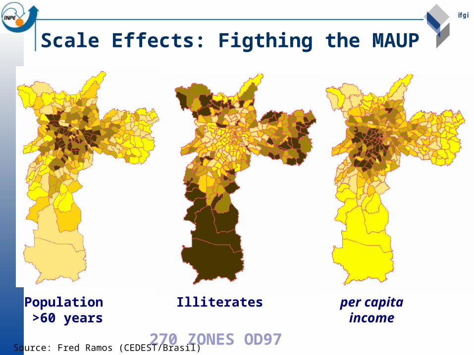
Population >60 years
Illiterates per capitaincome
270 ZONES OD97
Scale Effects: Figthing the MAUP
Source: Fred Ramos (CEDEST/Brasil)

96 DISTRICTS OF SÃO PAULO
Scale Effects: Figthing the MAUP
Population >60 years
Illiterates per capitaincome
Source: Fred Ramos (CEDEST/Brasil)

96 INCOME-HOMOGENOUS ZONES IN SÃO PAULO
Scale Effects: Figthing the MAUP
Population >60 years
Illiterates per capitaincome
Source: Fred Ramos (CEDEST/Brasil)

27
0 Z
ON
ES
OD
97
96
DIS
TR
ICTS
96
IN
CO
ME-
AG
GR
EG
ATED
A) Percentage of population 60 year-old or more
B) Percentage of illiterate population
C) Per capita individual income
VARIABLES
Correlation matrices
Source: Fred Ramos (CEDEST/Brasil)

Get census data
Identify inter-tractvariation
Adaptation
Minimize the outlier effect
Reduce data variability
A Questão da EscalaA Questão da Escala

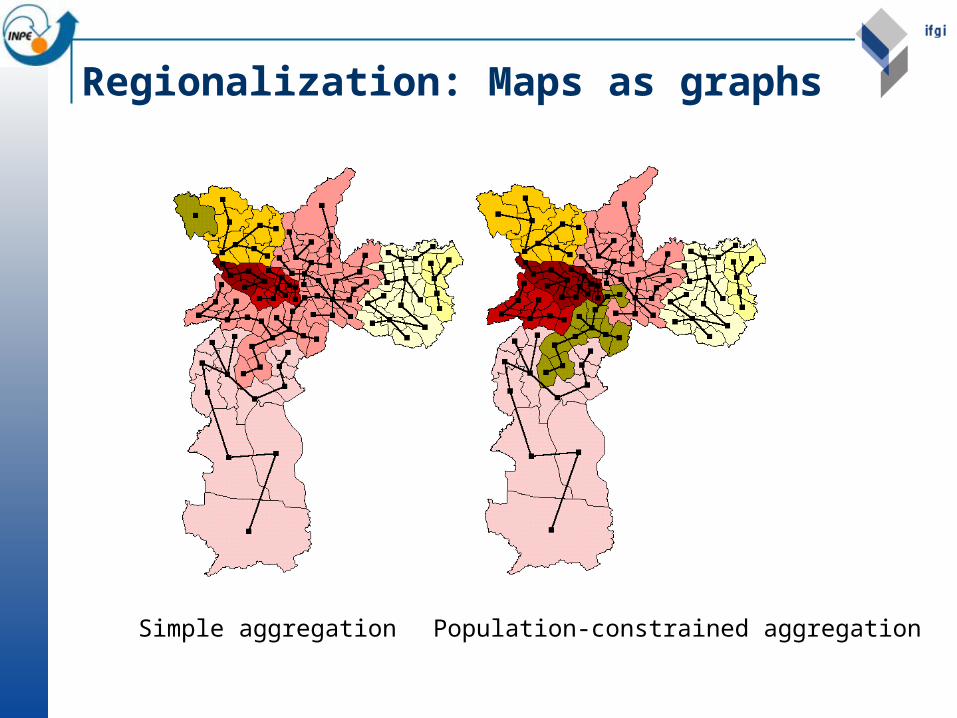
Regionalization
Reagregate N small areas (finest scale available) into M bigger regions to reduce scale effects.
A possible solution: constrained clustering

Regionalization: Maps as graphs
Regionalization: Maps as graphs
Simple aggregation Population-constrained aggregation
Top Related