


Languages
Pages
Legal

UNIVERSIDADE FEDERAL DE LAVRAS
SOME TOPICS IN PROCRUSTES
ANALYSIS APPLIED TO
SENSOMETRICS
ERIC BATISTA FERREIRA
2007
Ficha Catalográflca Preparada pela Divisão de Processos Técnicos daBiblioteca Central da UFLA
Ferreira, Eric Batista.Some topics in Procrustesanalysis appiied to Sensometrics/ Eric Batista
Ferreira. ~ Lavras : UFLA, 2007.
131 p. :il.
Tese (Doutorado) - Universidade Federal de Lavras, 2007.Orientador: Marcelo Silva de Oliveira.
Bibliografia.
1. Procrustes. 2. Sensorial analysis. 3. Missing values. 4. Bootstrapping. I.Universidade Federal de Lavras. II. Título.
CDD-519.535
ERIC BATISTA FERREIRA
Some topics in Procrustes analysis appiied to
Sensometrics
Tese apresentada à Universidade Fed
eral de Lavras, como parte das exigências do Programa de Pós-graduaçãoem Estatística e ExperimentaçãoAgropecuária, para obtenção do título de "Doutor".
Orientador: Prof. Dr. Marcelo Silva de Oliveira
BIBLIOTECA CENTRAL
UFLA
n° clasX5j13a.53.&.ftER
N° REGISTRO „^3% bftffDATA l3._../ CUl /flg .
LAVRAS
MINAS GERAIS - BRASIL
2007

ERIC BATISTA FERREIRA
Some topics in Procrustes analysis appiied toSensometrics
Tese apresentada à Universidade Federal deLavras, como parte das exigências do Programa de Pós-graduação em Estatística e Experimentação Agropecuária, para obtençãodo título de "Doutor".
APROVADA em 13 de novembro de 2007.
Prof. Dr. Daniel Furtado Ferreira
Proí*. Dra. Rosemary Gualberto F. A. Pereira
Prof. Dr. Fernando Antônio Resplande Magalhães
Prof. Dr. Renato Ribeiro ie Lima
Prof. Dr. Majrçeio SilvaMeiÓliveiraUFLA
(Orientador)
LAVRAS
MINAS GERAIS - BRASIL
UFLA
UFLA
EPAMIG
UFLA

PARA LUCIVANE
NÃO PODERIA TER ENCONTRADO TAMANHA DEDICAÇÃO EAMOR EM OUTRA PESSOA.

AGRADECIMENTOS
(ACKNOWLEDGEMENTS)
Embora não consiga listar o nome de todos aqueles que merecemser agradecidos e embora o faça misturando duas línguas, seguem meusprincipais agradecimentos.
Agradeço a Deus. Agradeço a minha família. Minha esposa, Luci-vane, pela compreensão, paciência e orações nos momentos mais difíceis deausência, principalmente durante o período que passei na Inglaterra. Meuspais, Rui e Marilene, pelo apoio incondicional e por nunca duvidarem demim. Minha irmã, Ester, pela admiração e apoio. Meus tios, avós, primos,sogros, sobrinhos e cunhados que, mesmo distantes, torceram e torcem pormim.
Agradeço a meus amigos. Para não correr o risco de esquecer decitar pessoas importantes, me reservo ao direito de agradecer meus colegasde Pós-graduação do DEX/UFLA e da Open University (Milton Keynes,UK), meus professores, meus amigos do Karate Kyokushin, meus amigosda banda Doravante e Ensaio Aberto, meus alunos e ex-alunos da UFLA,do UNIFOR e da UNIFAL-MG, meus amigos de Juiz de Fora, Lavras,Piúma, Alfenas, Formiga, Milton Keynes (UK) e tantas outras cidades pelasquais passei durante meu doutorado; e, nominalmente, Fabyano, Denis-mar, Washington e Beijo, que são como irmãos para mim; e a todos osfuncionários do DEX/UFLA.
Agradeço particularmente, a cinco pessoas que, para mim, são e-xemplos de vida e profissionalismo 1:
• Professor e amigo Daniel Furtado Ferreira, pela enorme lição de comodeve ser um cientista ético, dedicado e produtivo;
• Professor e amigo Eduardo Bearzoti, pelo exemplo de disciplina, éticae brilhantismo profissional, e, acima de tudo, por ensinar que nuncaé tarde para realizarmos nossos sonhos.
• Professor e amigo Fernando Antônio Resplande Magalhães, por terme apresentado a UFLA e Lavras, pela amizade, pelos conselhos, peloexemplo de profissional da área de Análise Sensorial, pelo carinho econsideração;
Listados em ordem alfabética.

• Professor and friend John Clifford Gower, for the friendship, for treat-ing me so well in a foreign land, for being an exemple to be followedof brilliant Mathematician and Statistician and for the great help inexploring missing value problems in Procrustes Analysis.
• Professor e amigo Marcelo Silva de Oliveira, pela lição de humanismoe sensibilidade no fazer científico e na enorme confiança que depositouem mim durante ambos mestrado e doutorado;
Agradeço a Capes (Coordenação de Aperfeiçoamento de Pessoal deNível Superior), por fomentar o meu doutorado e proporcionar minha temporada na Inglaterra para aprimorar meus conhecimentos e ter experiênciaspessoais e profissionais inesquecíveis.
Agradeço ao CNPq (Conselho Nacional de Desenvolvimento Científico e Tecnológico) por me dar a oportunidade de prosseguir minhaspesquisas em Sensometria no Pós-doutorado.
I thank the Open University, for kindly receiving me and contribut-ing to my human and technical formation.
E, finalmente, agradeço a minha querida Universidade Federal deLavras (UFLA) que, além de me proporcionar a graduação, o mestrado e odoutorado, me acolheu como filho em seu leito de conhecimento e tradição.Me sinto honrado em defender minha tese em meio as comemorações docentenário dessa Instituição de prestígio nacional e internacional.
Por meu respeito, amor e admiração à UFLA, publico aqui o hinoque compus para essa Instituição, que ficou colocado em quarto lugar noConcurso do Hino da Universidade Federal de Lavras, realizado em 2002.
Hino à Universidade Federal de Lavras
De um sonho estrangeiro gerada e criada com orgulho nacionalAbençoa a cidade de Lavras com a graça e glória da ESAL.
Com empenho de tantos amores, a benção de Deus e o rufar dos coraçõesSurge a UFLA repleta de cores contemplando as novas gerações.
Tu consegues respeito dosfilhos e dos mestres tens admiraçãoTu ajudas o homem do campo a desempenhar melhor sua junção.
A ciência que tanto praticas eleva teu nome e de quem te seguiuEs a dama que mora em Minas, flor do coração do meu Brasil.
CONTENTS
List of Figures i
List of Tables iv
Resumo v
Abstract vi
1 INTRODUCTION 1
1.1 History of Procrustes 4
1.2 Definitions and notation 4
1.3 Review of Procrustes Problems 8
1.4 Sensorial Analysis 16
2 MISSING VALUES IN PROCRUSTES PROBLEMS .... 22
2.1 Orthogonal Procrustes Rotation 22
2.1.1 Missing values 24
2.1.2 Methodology 26
2.1.3 Results and discussion 30
2.1.3.1 Exact match 30
2.1.3.2 Real sized error 34
2.1.4 Conclusions (A) 36
2.2 GeneraÜsed Procrustes Analysis (GPA) 38
2.2.1 Considerations about non-orthogonal GPA 40
2.2.2 General transformation 41
2.2.3 Orthogonal transformation 53
2.2.4 Algorithm 55
2.2.5 Conclusions (B) 56
3 STATISTICAL INFERENCE AND GPA 57
3.1 Introduction 57
3.2 Sampling in Sensory Sciences 60
3.3 GeneraÜsed Procrustes Analysis 62
3.4 Describing an object 63
3.5 Comparing objects 66
3.6 GPA and Inference 68
3.7 Monte Cario simulation 69
3.8 Permutation tests 70
3.9 Bootstrapping 71
3.9.1 Confidence regions estimation 72
3.9.2 Hypothesis testing 74
3.10 Methodology 75
3.10.1 Estimation 78
3.10.2 Decision 82
3.10.3 Algorithm 85
3.10.4 Practical experiments 86
3.10.5 Simulation studies 87
3.11 Results 91
3.11.1 Practical experiments 91
3.11.2 Simulation studies 105
3.12 Discussion 111
4 FINAL CONSIDERATIONS 113
Appendix A - PROOFS 114
Appendix B - R FUNCTIONS 124
References 126
LIST OF FIGURES
1 Origin and progress of Procrustes analysis and its main re-lated áreas 2
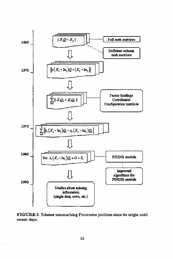
2 Scheme summarizing Procrustes problem since its origin un-til recent days 15
3 lUustration of rotating a matrix X\ to fit X%, in order to showthe corresponding vértices. Source: Commandeur (1991). . 23
4 Scheme of the distances (RSS) between X\ (before rotation)and the unknown full data X2 and the possible arbitrary con-figurations X$\ (i = 1,2,3,4,...) according to the putativevalues chosen 25
5 Behaviour ofparameter (a) u and (b) R2 along an increasingrate of missing values, when their putative values come fromGaussian (*) and Uniform (o) distributions and a fixed scalar(A) 32
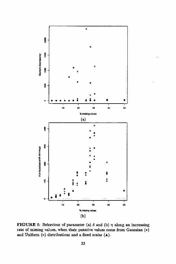
6 Behaviour of parameter (a) ô and (b) 77 along an increasingrate of missing values, when their putative values come fromGaussian (*) and Uniform (o) distributions and a fixed scalar(A) 33
7 Behaviour of parameter <p along an increasing rate of missingvalues, when their putative values come from Gaussian (*)and Uniform (o) distributions and a fixed scalar (A) 34
8 Behaviour of parameter (a) u and (b) R? along an increasingrate of missing values, when their putative values come fromGaussian (*) and Uniform (o) distributions and a fixed scalar(A) 35
9 Behaviour of parameter (a) 6 and (b) 77 along an increasingrate of missing values, when their putative values come fromGaussian (*) and Uniform (o) distributions and a fixed scalar(A) 37
10 Behaviour of parameter <f> along an increasing rate of missingvalues, when their putative values come from Gaussian (*)and Uniform (o) distributions and a fixed scalar (a) 38
11 (a) Relative euclidian distances between objects A, B e C.(b) Euclidian distances between objects D and E 58
12 Configurations for four objects (Oi,...,O4) 63
13 Configurations ofthree assessors (X\, X2 e X3) 64
14 Scores of five assessors to one object according to a pair ofattributes: generation of a sensorial space (Í2<p), Sensu of theobject (*) and its estimates ($1, tf2, $3, *4 e #5) 65
15 Score of four assessors (i = 1,... ,4) to three objects (Z =1,..., 3), with respect to two main attributes: generation ofa sensorial space (Í2*), Sensu of the three objects (ty) andtheir respective estimates ($/*) 67
16 (a) Sensorial confidence region for one object comprising1007% of the data generated by resampling one group av-erage configuration ('mean' scores through assessors). (b)lUustration of the bootstrap distance between supposed objects F and G 77
17 (a) Estimate of a 95% confidence region base on bivariatenormal distribution. (b) Estimate of a 95% confidence region base on bivariate histogram estimator; for the samehypothetic cloud of points 81
18 lUustration of an empirical distribution (set of ordered values 6b) and highlight on a possible location of the samplereference value (5r) 83
19 Flowchart for the proposed methodology. 84
20 lUustration scheme of the second simulation study. 89
21 Transformed scores for eight products (1 to 8), by nine assessor (A to J), on the response-plane of GPA 92

22 (a) Estimated bootstrap confidence regions for the 8 cheeses.Bootstrap estimates are in black and the sample estimate inwhite. (b) Same scene hiding the bootstrap estimates andhighUghting the 95% confidence region. Attributes positionare highlighted 93
23 Empirical distribution of the euclidian distances based on500 bootstrap estimates under the nuU hypothesis. (a) fio :<51)6 = 0 and; (b) H0 : $3,7 = 0 94
24 Bar plots for attributes 1 to 10 of Gorgonzola experiment.(a) Highlights C statistics and (b) their logarithm 97
25 Scree plot for attributes 1 to 10 in Gorgonzola experiment. 98
26 Assessors space for attributes 10 - residual flavor (a) and 9 -bitter taste (b) 99
27 Two first principal axis, highlighting 95% confidence eUipsesand attributes, for experiments (a) and (b) with comercialdairy products in The Netherlands 101
28 (a) Bar plot of the statistic C and; (b) scree plot for thefirst four dimensions, of ali nine attributes of experiment 1of Dutch comercial products 102
29 (a) Bar plot of the statistic C and; (b) scree plot for thefirst four dimensions, of ali nine attributes of experiment 2of Dutch comercial products 103
30 Assessors' space for the most and the less unidimensionalattribute of Dutch experiment 1, respectively attributes 3(a) and 6 (b) 104
31 Assessors' space for the most and the less unidimensionalattribute of Dutch experiment 2, respectively attributes 2(a) and 9 (b) 106
32 (a) Randomly chosen estimation biplot for iUustrating thereplication of the simulation process based on Gorgonzolaparameters estimates. (b) Box plots for variance accountedfor (VAF) for 10 principal components and sample estimate,represented by a x 108
111

LIST OF TABLES
1 Meaning of the term Procrustes along some áreas of knowledge. 3
2 Comparison of human basic senses according to the numberof discernible stimuli, sharpness of discrimination, averagespeed of reaction and duration of sensation (adapted fromAmerine et ai., 1965) 17
3 Simulated loss in X\, X2 and in both matrices, expressed asa percentage of the cells 27
4 The Índices of the missing cells 44
5 Tabular representation of scores from k assessors to one object according to p attributes (xíj) 64
6 Tabular representation of scores for n objects, under p attributes, given by the ith judge 66
7 Power and type I error rates (R\ to Rs) for both estimationand decision stages, under partial Hq, for virtual paneis ofsizes 5, 10, 15, 20, 50 and 90 109
8 Variances accounted for the first five principal componentsand their standard deviations along the simulated sample sizes.lll
IV
RESUMO
FERREIRA, Eric Batista. Alguns tópicos em Análise de Procrustesaplicada à Sensometria. Lavras: UFLA, 2007. 131 p. (Tese - Doutoradoem Estatística e Experimentação Agropecuária)*
Os problemas de Procrustes são estudados desde a segunda metadedo século XX, quando o primeiro problema foi proposto. Desde então aAnálise de Procrustes foi muito estudada e desenvolvida. Contudo ainda
persistem lacunas como o estudo da estimação de parcelas perdidas e afalta de ferramentas de Inferência Estatística. O presente trabalho estudaa influência dos chutes iniciais na estimação de parcelas em problemas ordinários de Procrustes, relata e propõe novos aspectos em algoritmos deestimação em problemas generalizados de Procrustes e descreve uma proposta de método decisório para permitir a Inferência em tal análise. Essemétodo é ilustrado com três experimentos reais e dois estudos de simulação de dados. Os chutes iniciais mostram interferência no resultado dosajustes e o método decisório se mostrou coerente, estável e eficiente na detecção de produtos semelhantes, associando uma fase liberal com uma faseconservativa.
Comitê orientador: Marcelo Silva de Oliveira - UFLA (orientador); Daniel FurtadoFerreira (UFLA) e John Clifford Gower (Open University).

ABSTRACT
FERREIRA, Eric Batista. Some topics in Procrustes analysis appiiedto Sensometrics. Lavras: UFLA, 2007. 131 p. (Thesis - PostgraduationProgram in Statistics and Agricultura! Experimentation)*
Procrustes problems have been studied since the second half of the20th century, when the first problem was stated. Since then Procrustesanalysis has been developed. However, some gaps still hold mainly in esti-mating missing values and the lack of tools for statistical inference. Thiswork analises the influence of putative values in the estimation of missingcells in ordinary Procrustes problems, reports and suggest new aspects forestimation algorithms in generalised Procrustes analysis and describes a de-cision method to allow inference features. Such method is illustrated with
three practical experiments and two simulation studies. Inadequate putative values have shown to ability to lead to local minima and the decisionmethod performed coherently, stably and efficiently in detecting similarproducts, associating a liberal and a conservative stage.
Guidance committee: MarceloSilvade Oliveira- UFLA (supervisor); Daniel FurtadoFerreira (UFLA) and John Clifford Gower (Open University).
vi
1 INTRODUCTION
Hurley & Cattell (1962) did a homage to Procrustes, personage of
Greek mythology, when they used his name, for the first time, to refer to
a minimization problem that intended to transform a given matrix into
another. Depending on how that minimization problem is set it receives a
particular name, setting up a particular Procrustes problem.
Besides the importance on itself, i.e., on solving how two (set of) ma
trices best fit themselves only using some allowed transformations, the Pro
crustes problems have found a crucial role in sensorial sciences. Williams
& Langron (1984), for instance, stated a sensorial methodology called Free
Choice Profiling (FCP), only possible after the progress of the Procrustes
analysis. On the other hand, the development of FCP certainly motivated
the Procrustes problems to keep in progress (Figure 1). Free Choice Pro
filing allow each assessor to score his/her own set of attribute, in his/her
own scale. That is what the Procrustes problems are ali about, comparing
configurations apart from bias of scaling, positioning or orientation.
So many others áreas of science have used and have been influenced
by Procrustes apart from sensorial sciences. Particularly, Statistical Shape
Analysis uses Procrustes rotation from so long ago (Ian Dryden) and is the
another important application of Procrustes analysis. However, it can be
found a lot of others áreas where Procrustes have been used, like Paleon-
tology (Rodrigues & Santos, 2004), Medicine (Rangarajan, 2003), Ecology
(Moraes, 2004), Molecular genetics (Mironov et ai., 2004), automotive in-
dustry (Dairou et ai., 2004) and Photogrammetry (Akca, 2003).
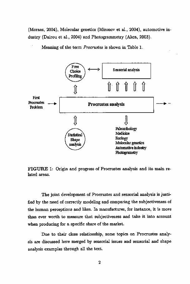
Meaning of the term Procrustes is shown in Table 1.
First
Procrostes
Problem
< > Sensorial analysis
M t t í
Procrustes anatvsis
íPateonlhologyMedicine
EcologyMolecular geneticsAutomotive industryPhotogrametn'
FIGURE 1: Origin and progress of Procrustes analysis and its main re-lated áreas.
The joint development of Procrustes and sensorial analysis is justi-
fied by the need of correctly modeHng and comparing the subjectiveness of
the human perceptions and Ukes. In manufactures, for instance, it is more
than ever worth to measure that subjectiveness and take it into account
when producing for a specific share of the market.
Due to their close relationship, some topics on Procrustes analy
sis are discussed here merged by sensorial issues and sensorial and shape
analysis examples through ali the text.
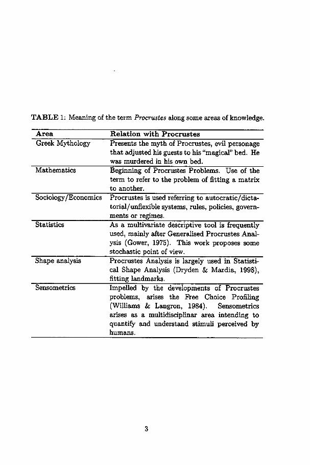
TABLE 1: Meaning of the term Procrustes along some áreas of knowledge.
Área
Greek Mythology
Mathematics
Sociology/Economics
Statistics
Shape analysis
Sensometrics
Relation with Procrustes
Presents the myth of Procrustes, evil personagethat adjusted his guests to his "magical" bed. Hewas murdered in his own bed.
Beginning of Procrustes Problems. Use of theterm to refer to the problem of fitting a matrixto another.
Procrustes is used referring to autocratic/dicta-torial/unflexible systems, rules, policies, govern-ments or regimes.As a multivariate descriptive tool is frequentlyused, mainly after Generalised Procrustes Analysis (Gower, 1975). This work proposes somestochastic point of view.Procrustes Analysis is largely used in Statisti-cal Shape Analysis (Dryden & Mardia, 1998),fitting landmarks.Impelled by the developments of Procrustesproblems, arises the Free Choice Profiling(Williams & Langron, 1984). Sensometricsarises as a multidisciplinar área intending toquantify and understand stimuli perceived byhumans.

1.1 History of Procrustes
Procrustes is a Greek Mythology personage. Son of Poseidon, he
had a special bed in his chamber that would have the power to adjust
itself to anyone laid on it. Procrustes use to offer a great banket to the
peregrines that passed by his chamber, full of food and wine. After the
dinner, he offered a restful night on a magical bed. When they had no way
out he announced that they should exactly fit his, what never happened.
Just in case, he had two beds to ensure anyone would never fit it. In order
to fit the guest to the bed, Procrustes stretched or racked his legs and
arms. However, Procrustes had a tragic fait. Theseus, in his way to claim
Athens reign, killed him on his own bed, as one of his six works. Hurley &
Cattell (1962) did homage to that Greek Mythology personage stating the
Procrustes problem, a mathematical fitting problem, for the first time.
Procrustes myth seems to denounce one (or several) human blem-
ish(es): the intolerance (besides rigidity and cruelty). It denounces a dark
side of human beings that tends to impose its will at any cost, in spite of
chopping and stretching.
1.2 Definitions and notation
In this section some basic definitions are presented and the notation
adopted along the text is stated.
Reading the following definitions, consider that, mainly in gener
alised Procrustes problems, some definitions use index i to refer to several
matrix (e.g. Xi, i = 1,..., k).
Moreover, along the text, the sign ' denotes transposed matrices
(e.g. X' is X transposed); tr stands for the trace ofa matrix (e.g. tr(A) =trace{A))\ and the sign * denotes the element-wise product of two matrices.
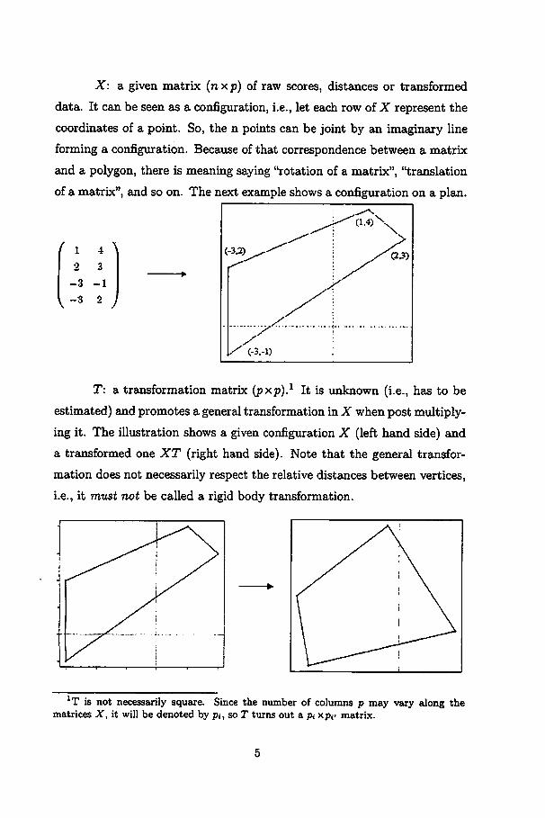
X: a given matrix (nxp) of raw scores, distances or transformed
data. It can be seen as a configuration, i.e., let each row of X represent the
coordinates of a point. So, the n points can be joint by an imaginary line
forming a configuration. Because of that correspondence between a matrix
and a polygon, there is meaning saying "rotation of a matrix", "translation
of a matrix", and so on. The next example shows a configuration on a plan.
/ 1 4 \2 3
-3 -1
-3 51 J
T: a transformation matrix (pxp).1 It is unknown (i.e., has to be
estimated) and promotes a general transformation in X when post multiply-
ing it. The illustration shows a given configuration X (left hand side) and
a transformed one XT (right hand side). Note that the general transfor
mation does not necessarily respect the relative distances between vértices,
i.e., it must not be called a rigid body transformation.
lT is not necessarily square. Since the number of columns p may vary along thematrices X, it will be denoted by p*, so T turns out a p< xpj/ matrix.
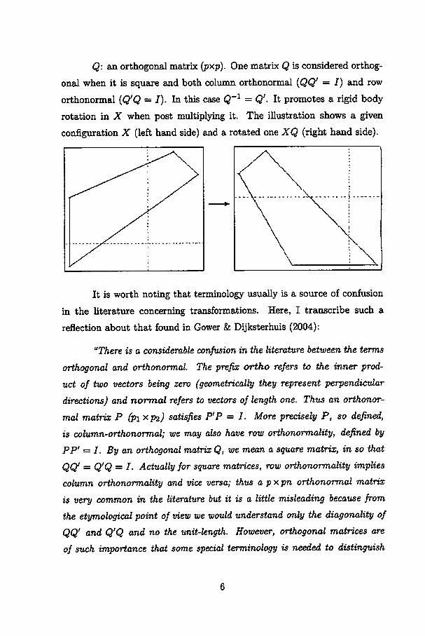
Q: an orthogonal matrix (pxp). One matrix Q is considered orthog
onal when it is square and both column orthonormal {QQ' = I) and row
orthonormal {Q'Q = J). In this case Q'1 = Q'. It promotes a rigid body
rotation in X when post multiplying it. The illustration shows a given
configuration X (left hand side) and a rotated one XQ (right hand side).
It is worth noting that terminology usually is a source of confusion
in the literature concerning transformations. Here, I transcribe such a
reflection about that found in Gower & Dijksterhuis (2004):
"There is a considerable confusion in the literature betweenthe terms
orthogonal and orthonormal. The preftx ortho refers to the inner prod-
uct of two vectors being zero (geometrically they represent perpendicular
directions) and normal refers to vectors of length one. Thus an orthonor
mal matrix P (p\ XP2) satisfies P'P = /. More precisely P, so defined,
is column-orthonormal; we may also have row orthonormality, defined by
PP' = J. By an orthogonal matrix Q, we mean a square matrix, in so that
QQ' = Q'Q = I. Actually for square matrices, row orthonormality implies
column orthonormality and vice versa; thus a pxpn orthonormal matrix
is very common in the literature but it is a little misleading because fromthe etymological point of view we would understand only the diagonality of
QQ' and Q'Q and no the unit-length. However, orthogonal matrices are
of such importance that some special terminology is needed to distinguish
them from non-square orthonormal matrices. In the literature, what we
call orthonormal matrices are sometimes described as orthogonal, which is
etymologically correct but a source of confusion. Another source of confu
sion in the literature is that quite general matrices T may be referred to
as representing rotations whereas, strictly speaking, rotation only refers to
orthogonal matrices and then not ali orthogonal matrices."
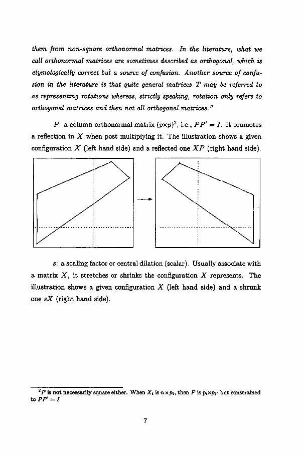
P: a column orthonormal matrix (pxp)2, i.e., PP' = /. It promotes
a reflection in X when post multiplying it. The illustration shows a given
configuration X (left hand side) and a reflected one XP (right hand side).
s: a scaling factor or central dilation (scalar). Usually associate with
a matrix X, it stretches or shrinks the configuration X represents. The
illustration shows a given configuration X (left hand side) and a shrunk
one sX (right hand side).
2P is not necessarily square either. When Xi isn xp<, then P ispixpv but constrainedto PP' = /
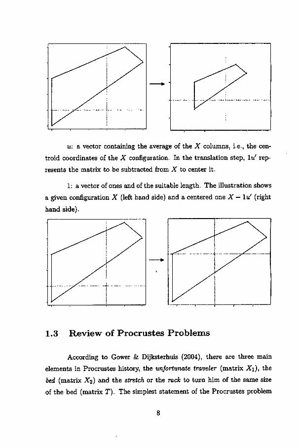
u: a vector containing the average of the X columns, i.e., the cen-
troid coordinates of the X configuration. In the translation step, lu' rep-
resents the matrix to be subtracted from X to center it.
1: a vector of ones and of the suitable length. The illustration shows
a given configurationX (left hand side) and a centered one X —lu' (right
hand side).
1.3 Review of Procrustes Problems
According to Gower & Dijksterhuis (2004), there are three main
elements in Procrustes history, the unfortunate traveler (matrix Xi), the
bed (matrix X2) and the stretch or the rack to turn him of the same size
of the bed (matrix T). The simplest statement of the Procrustes problem
8
seeks for a matrix T to minimize
\\XiT-X2%
where T is a matrix with dimensionality p\ x p2\ X\ and X2 are given
matrices with dimensionality n x pi and (n x P2), respectively; and || • ||
denotes the Euclidean/Frobenius norm, that is ||A|| = trace{A'A). In
sensorial analysis, those quantities can be understood as: n, number of
evaluated objets; p\, number of variables used by assessor 1 to evaluate
such objects; P2, number of variables used by assessor 2. Note that, since
T is a general matrix, if X\ is invertible, there is a matrix T = Xf1A*2which is a ready solution for the problem, i.e., there is T such that X\
fits exactly X2. But, in order to T equals X^X2, it is necessary X\ tobe invertible, that is, X must be a square matrix and must have non-zero
determinant. In general, X\ neither is square nor is guaranteed to have
non-zero determinant. So, the minimization problem proceeds.
x{1)
x(1)L xnl
.(D i r'1P1
z(1) t 1
*11 1P2
tPlP2 J
rT(2)
x(2)L xn\
.(2)'1P2
x{2)Xnp2
The minimization problem is called a Procrustes problem because
X\ is transformed by T to best fit X2. Under that ordinary point of view,
T is unrestricted real matrix. According to Gower & Dijksterhuis (2004),
that is a multivariate multiple regression problem (1.1). Therefore, one can
derive a least squares estimator3 of T.
3Demonstrationin (A.l).
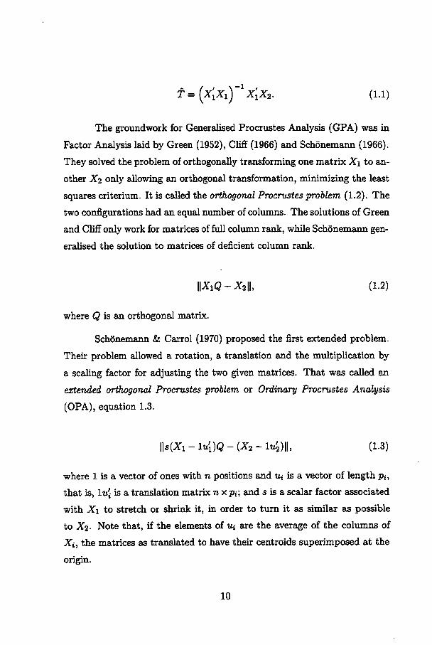
=(*í*l) lx[x2. (1.1)
The groundwork for Generalised Procrustes Analysis (GPA) was in
Factor Analysis laid by Green (1952), Cliff (1966) and Schõnemann (1966).
They solved the problem of orthogonally transforming one matrix X\ to an
other X2 only allowing an orthogonal transformation, minimizing the least
squares criterium. It is called the orthogonal Procrustes problem (1.2). The
two configurations had an equal number of columns. The solutions of Green
and Cliff only work for matrices of full column rank, while Schõnemann gen
eralised the solution to matrices of deficient column rank.
\\XlQ-X2\l (1.2)
where Q is an orthogonal matrix.
Schõnemann & Carrol (1970) proposed the first extended problem.
Their problem allowed a rotation, a translation and the multiplication by
a scaling factor for adjusting the two given matrices. That was called an
extended orthogonal Procrustes problem or Ordinary Procrustes Analysis
(OPA), equation 1.3.
IWJfi-ltti)Q-(X2-lt4)H, (1.3)
where 1 is a vector of ones with n positions and uí is a vector of length pi,
that is, lUi is a translation matrix nxpi; and 5 is a scalar factor associated
with X\ to stretch or shrink it, in order to turn it as similar as possible
to X2. Note that, if the elements of it» are the average of the columns of
Xi, the matrices as translated to have their centroids superimposed at the
origin.
10
Gower (1971) had taken the first steps towards the generalised or
thogonal Procrustes analysis (GPA or GOPA). In that context, X\ and
X2 are replaced by k sets X\,..., Xk- This may have been the first in
stance where the matrices X\,...,Xk are regarded as configuration matri
ces rather than as coordinates matrices of factor loadings (Gower & Dijk-
sterhuis, 2004).
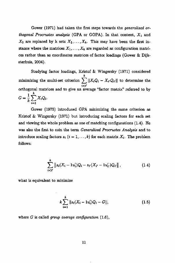
Studying factor loadings, Kristof & Wingersky (1971) consideredk
minimizing the multi-set criterion ^||XiQt - AVQi/|| to determine the
orthogonal matrices and to give an average "factor matrix" referred to by
i=l
Gower (1975) introduced GPA minimizing the same criterion as
Kristof & Wingersky (1971) but introducing scaling factors for each set
and viewing the whole problem as one of matching configurations (1.4). He
was also the first to coin the term Generalised Procrustes Analysis and to
introduce scaling factors Si (i = 1,..., k) for each matrix Xi. The problem
follows:
53 \\sí(Xí - lu^Qi - Si,(Xi, - lu;,)<3i<||, (1.4)
what is equivalent to minimize
k
k^WsiiXi-lu^Qi-GH (1.5)
where G is called group average configuration (1.6),
11
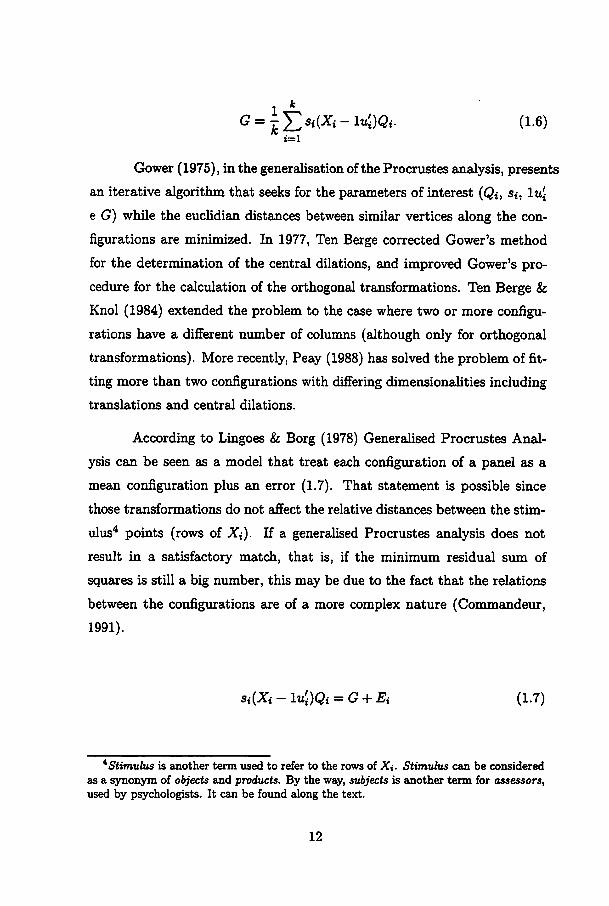
1 *<? =£]£>(*-ltiJWi. (1-6)
t=i
Gower (1975), in the generalisation of the Procrustes analysis, presents
an iterative algorithm that seeks for the parameters of interest (Q», s,, lwj
e G) while the euclidian distances between similar vértices along the con
figurations are minimized. In 1977, Ten Berge corrected Gower's method
for the determination of the central dilations, and improved Gower's pro-
cedure for the calculation of the orthogonal transformations. Ten Berge &
Knol (1984) extended the problem to the case where two or more configu
rations have a different number of columns (although only for orthogonal
transformations). More recently, Peay (1988) has solved the problem of fit
ting more than two configurations with differing dimensionalities including
translations and central dilations.
According to Lingoes & Borg (1978) Generalised Procrustes Anal
ysis can be seen as a model that treat each configuration of a panei as a
mean configuration plus an error (1.7). That statement is possible since
those transformations do not affect the relative distances between the stim-
ulus4 points (rows of Xi). If a generalised Procrustes analysis does not
result in a satisfactory match, that is, if the minimum residual sum of
squares is still a big number, this may be due to the fact that the relations
between the configurations are of a more complex nature (Commandeur,
1991).
Sí{Xí-\u'í)Qí = G+ Eí (1.7)
AStvmvXus is another term used to refer to the rows of Xi. Stimulus can be consideredas a synonym of objects and products. By the way, subjects is another term for assessors,used by psychologists. It can be found along the text.
12
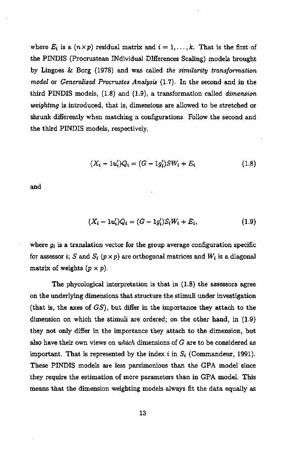
where Ei is a (nxp) residual matrix and i = 1,..., k. That is the first of
the PINDIS (Procrustean INdividual DIfferences Scaling) models brought
by Lingoes & Borg (1978) and was called the similarity transformation
model or Generalised Procrustes Analysis (1.7). In the second and in the
third PINDIS models, (1.8) and (1.9), a transformation called dimension
weighting is introduced, that is, dimensions are allowed to be stretched or
shrunk differently when matching n configurations. Follow the second and
the third PINDIS models, respectively,
(Xi - Iu'í)Qí = (G- ifàSWi + Ei (1.8)
and
(Xi - Iu'í)Qí = (G- \g'dSiWi + Eu (1.9)
where pt- is a translation vector for the group average configuration specific
for assessor i; S and Si (pxp) are orthogonal matrices and W, is a diagonal
matrix of weights (pxp).
The phycological interpretation is that in (1.8) the assessors agree
on the underlying dimensions that structure the stimuli under investigation
(that is, the axes of GS), but differ in the importance they attach to the
dimension on which the stimuli are ordered; on the other hand, in (1.9)
they not only differ in the importance they attach to the dimension, but
also have their own views on which dimensions of G are to be considered as
important. That is represented by the index i in Si (Commandeur, 1991).
These PINDIS models are less parsimonious than the GPA model since
they require the estimation of more parameters than in GPA model. This
means that the dimension weighting models always fit the data equally as
13
well as or better than the GPA model.
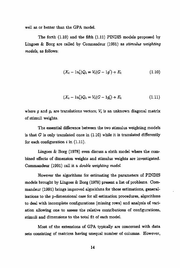
The forth (1.10) and the fifth (1.11) PINDIS models proposed by
Lingoes & Borg are called by Comnandeur (1991) as stimulus weighting
models, as follows:
(Xi - lu'i)Qi = Vi(G - lg') + Ei (1.10)
(Xi - \u'í)Qí = Vi(G - lg[) + Ei (1.11)
where g and gi are translations vectors; Vi is an unknown diagonal matrix
of stimuli weights.
The essential difference between the two stimulus weighting models
is that G is only translated once in (1.10) while it is translated differently
for each configuration i in (1.11).
Lingoes & Borg (1978) even discuss a sixth model where the com-
bined effects of dimension weights and stimulus weights are investigated.
Commandeur (1991) call it a double weighting model.
However the algorithms for estimating the parameters of PINDIS
models brought by Lingoes & Borg (1978) present a list of problems. Com
mandeur (1991) brings improved algorithms for those estimations, general-
isations to the p-dimensional case for ali estimation procedures, algorithms
to deal with incomplete configurations (missing rows) and analysis of vari-
ation allowing one to assess the relative contributions of configurations,
stimuli and dimensions to the total fit of each model.
Most of the extensions of GPA typically are concerned with data
sets consisting of matrices having unequal number of columns. However,
14
1960
1970
1975
1980
1990
!!*£-*, I
o\\s(xl-í^)Q-(X1-iu2
ü
ot
Ex:si(Xi-lui)Q=G+Et
a.Studies about missing
niformation
(single data. rows, efc.)
Fuli rank matrices
Defictent cohram
rank matrices
Factor loadingsCoordmates
Configuration matrices
PINDIS models
ImprovedálgCTÍÜnns for
PINDIS models
FIGURE 2: Scheme summarizing Procrustes problem since its origin untilrecent days.
15
the case of different number of rows (that is, missing Information about
one or more stimuli) are mentioned by: (i) Everitt Sc Gower (1981) apud
Commandeur (1991), in the context of what they called a weighted gener
alised Procrustes method, where they did not incorporate central dilations;
and De Leeuw & Meulman (1986) apud Commandeur (1991); (ii) in Jack-
knife context, where they allowed only one missing stimulus per matrix.
Commandeur (1991) bring a matching procedure called MATCHALS that
allows any pattern of missing rows.
A scheme is presented in Figure 2 roughly summarizing the path of
Procrustes problems.
1.4 Sensorial Analysis
Sensorial analysis or Sensory analysis is a very wide field of the sci-
ence concerned to understand, describe, measure and/or even reproduce the
mechanisms of perception of externai stimuli by human basic senses. The
word sensorial comes from Latin sensus, which means sense (Anzaldua-
Morales, 1994).
Mueller (1966) says that the senses are our highways to the outside
world. Though that phrase is not very related to senses, it remind us that
the only way to perceive the world is through our basic senses. Everything
one knows besides his/her instincts carne to him/her by the basic senses
(Table 2).
Depending on how one looks to that system, it receives a different
name. For instance, when one wants to understand how a person perceives
an object (focus on the person), we are in the field of Psychology. It can
receive the name Sensory Psychology and/or Psychophysics when regards
the physiology of perception and physical phenomena related to perceiving
something (Mueller, 1966); and Experimental Psychology or Psychometrics,
16
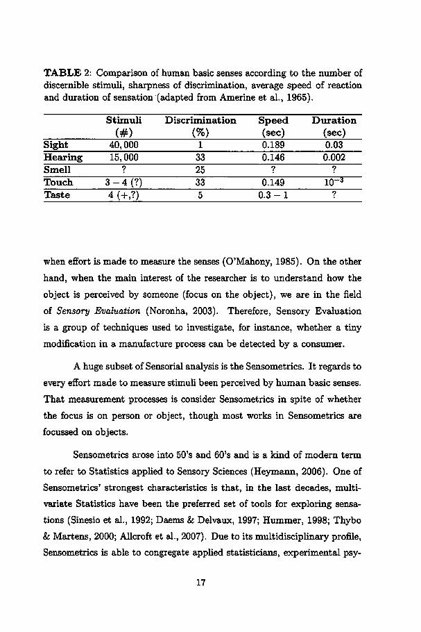
TABLE 2: Comparison of human basic senses according to the number ofdiscernible stimuli, sharpness of discrimination, average speed of reactionand duration of sensation (adapted from Amerine et ai., 1965).
Stimuli
(#)
Discrimination
(%)
Speed(sec)
Duration
(sec)Sight 40,000 1 0.189 0.03
Hearing 15,000 33 0.146 0.002
Smell ? 25 ? ?
Touch 3-4 (?) 33 0.149 IO"3
Taste 4 (+,?) 5 0.3-1 ?
when effort is made to measure the senses (0'Mahony, 1985). On the other
hand, when the main interest of the researcher is to understand how the
object is perceived by someone (focus on the object), we are in the field
of Sensory Evaluation (Noronha, 2003). Therefore, Sensory Evaluation
is a group of techniques used to investigate, for instance, whether a tiny
modification in a manufacture process can be detected by a consumer.
A huge subset of Sensorial analysis is the Sensometrics. It regards to
every effort made to measure stimuli been perceived by human basic senses.
That measurement processes is consider Sensometrics in spite of whether
the focus is on person or object, though most works in Sensometrics are
focussed on objects.
Sensometrics arose into 50's and 60's and is a kind of modera term
to refer to Statistics appiied to Sensory Sciences (Heymann, 2006). One of
Sensometrics' strongest characteristics is that, in the last decades, multi-
variate Statistics have been the preferred set of tools for exploring sensa-
tions (Sinesio et ai., 1992; Daems k Delvaux, 1997; Hummer, 1998; Thybo
& Martens, 2000; Allcroft et ai., 2007). Due to its multidisciplinary profile,
Sensometrics is able to congregate appiied statisticians, experimental psy-
17

chologists, food engineers, chemical engineers, mathematicians, physicists,
doctors, marketing people and so many other practitioners interested in
human senses.
Though Sensory Evaluation can be used to investigate how any kind
of object is perceived by human senses, its use is by fax greater in food
science (Ferreira, 2004; Jorge, 1989; Aquino, 1992; Aguiar, 1995; Cardoso,
1994; Malvino Madrid, 1994; Chagas, 1994; Magalhães, 2002).
However, other products can be studied regarding the sensations
they produce. For instance, automotive industry is an increasing field of
studies. Sensation of car breaks and interaction between consumer, car and
road have been studied by Dairou et ai. (2004) and Astruc et ai. (2006),
respectively. The cosmetic industry is also very developed due to constant
investigations of mainly odor and color perceptions (Wortel et ai., 2000;
MacDougall, 2000; Chrea et ai., 2004).
In a sensory context, in a large sense, a set of people evaluate a
set of objects. When those people are trained assessors or experts, they
are called a panei. When they are not trained at ali and are searched at
marketplace, they are called consumers. In that context, one even can
imagine degrees of training, i.e., people who are rapidly trained or even are
used to the sensory world, were trained before but not for the object at
issue. The prior can be understood, therefore, as a semi trained assessor.
At last, there are untrained people who are not asked for scoring objects
in their usual marketplaces (but anywhere else). Lets call them untrained
assessors.
How was said above, in Experimental Psychology the main focus
of the work is the person. So, attention has to be paid to the fact that
one is seeking for random samples of people, i.e., they should be random
elements of a population of interest for which conclusions and statements
are to be maid (0'Mahony, 1985). On the other hand, when a panei of
18

trained assessor or experts is used to evaluate something, it has to be clear
that it is not a random sample of a population of consumers. They were
screened from a population of consumers for been skillful, trained to be
able to precisely detect several sensorial attributes and distinguish between
products supposedly similar.
In the sensory evaluation of foods (or other products), there can
be more than one goal. In some situations, people may be used for a
preliminary analysis to measure an attribute of the food and provide clues
for later chemical or physical analysis. In others, they may be used to
measure, say, flavor changes due to a change in the processing of the food.
They can describe a product or compare a set of possible recipes to the
market leader. Consequently, assessors can be evaluated with respect to
the precision (variance), exactness, accuracy, i.e., success of the training
process. In turn, consumers can be used to evaluate preference for one
product rather than others, indicate the levei of that preference or even say
whether they would buy it.
Depending on how the group of assessors is chosen, the factor as
sessor can be assumed to be a fixed or a random effect. For instance, a
panei comprising of a few people is selected and trained to become judges in
the specific task required, whether it be detecting off-flavors in beverages
or rating the texture of cakes. That would be a fixed effect. Generally,
potential judges are screened to see whether they are suitable for the task
at issue. This careful selection of judges is in no way a random sampling
and is the first reason why the judges could not be regarded as representa-
tive of the population in general. The training then given to the selected
judges will usually make them more skilled in their task than the general
population would be; this is the second reason why they can no longer be
regarded as presentative of the population from which they were drawn.
Those judges are not a sample to be examined so that conclusions can be
19
drawn about a population; they are the population (0'Mahony, 1985).
Statistically thinking, a good training is expected to scale their mean
scores (vector of means, in a multivariate sense) closer to the parameter, i.e.,
remove possible natural bias specific for that person; and decreases their
variance (covariance matrix). Note that as a good training can remove the
bias more and more, a bad one can insert a bias not observed since then!
Considering the whole process of selection, training and scoring to
be an experiment, the panei can be considered a sample from a theoretical
population of trained assessors. That enables statistical inference. Usually,
this is not treated this way because the theoretical population of trained
assessors is kind of immaterial and judged as of low importance by some.
The panei is frequently consider the population itself and each assessor is
like a measurement instrument. 0'Mahony (1985) says that when the focus
of the study is very much on the food, the judges are merely instruments used
for measuring samples offood. Logically, one goodjudge would be adequate
for this purpose, as is one good gas chromatograph or atomic absorption
spectrometer. More than one judge is used as a precaution because unlike
a gas chromatograph, a judge can become distracted; the cautious use of
second opinion can provide a useful fail-safe mechanism. Apart from that,
one can consider that theoretical population particularly when dealing with
semi trained assessors.
On the other hand, if one wants to investigate how regular people
perceive a particular product, it can be done drawing untrained assessors
from the potential buying public (at the marketplace or not). Then from
this sample, inferences can be made about the population of untrained
people in general. The experiment now becomes similar to one in Sensory
Psychophysics.
In both cases, it is worth considering each assessor to be a block.
He/she has exactly the attributes of a block, like homogeneity within and
20
heterogeneity between scores. But the differences between considering ran
dom or fixed effects becomes important for analysis of variance, where dif
ferent denominators are used for calculating F values. Where conclusions
apply only to the judges tested, the judges are said to be a fixed effect.
Where conclusions apply to the whole population from which the judges
were drawn, the judges are said to be a random effect.
According to 0'Mahony (1985), in Psychology or Psychophysics,
people are the subject of the investigation and thus tend to be called sub-
jects. In sensory evaluation, or sensory analysis as it is also called, peo
ple are often specially selected and trained and tend to be referred to as
judges. In sensory analysis, judges are tested while isolated in booths; ex-
perimenters and judges communicate by codes, signs or writing. In Sensory
Psychophysics, the experimenter and subject often interact and communi
cate verbally; this requires special training for experimenters so that they
do not influence or bias on the subjects. The methods of sensory analy
sis are often derived from those of Psychophysics, but care must be taken
when adapting psychophysical tests to sensory evaluation. This is because
the goals of the two disciplines are different and they can affect the appro-
priateness of various behavioral methods of measurement used, as well as
the statistical analysis employed. In Psychophysics, the aim is to measure
the "natural" functioning of the senses and cognitive processes. Extensive
training will not be given if it alters a subject's mode of responding or
recalibrates the person, so obscuring his or her "natural" functioning.
21
MISSING VALUES IN PROCRUSTES
PROBLEMS
2.1 Orthogonal Procrustes Rotation
The minimization problem of transforming one given matrix Xi by
a matrix, say T, such that best fits a given target matrix X2 is called
a Procrustes Problem. The term Procrustes Problem is due to Hurley &
Cattel (1962) whose suggested the problem of transforming one matrix into
another by minimizing the Residual Sum of Squares (RSS)
\\XiT-x2\\
for the first time. Here, T refers to a general transformation matrix but
Schõnemann (1966) solved that problem for a restricted case where Q,
instead of T, is orthogonal. Of course, when there are no restrictions, that
problem can be solved as a multivariate multiple regression, i.e.,
T = (XÍX1)-1X'1X2.
In the orthogonal case, i.e., when the general transformation T is replaced
by an orthogonal matrix Q, that problem is called Orthogonal Procrustes
Rotation (OPR). In fact, if one consider that the post multiplication by
an orthogonal matrix is itself a rotation (Gower & Dijksterhuis, 2004),
that term could be consider a pleonasm. The terms Procrustes Rotation
(PR) or Ordinary Procrustes Rotation (OPR), where Ordinary refers to
22
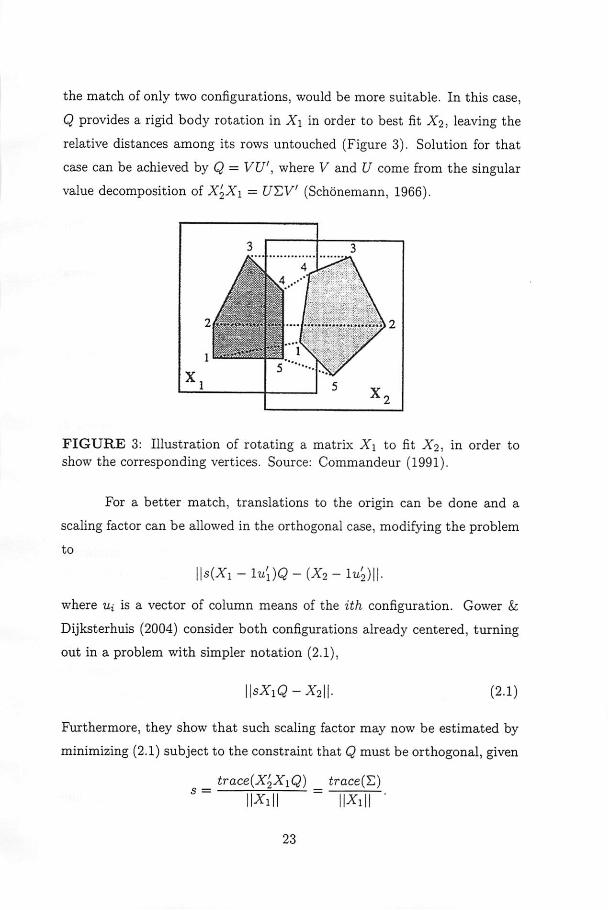
the match of only two configurations, would be more suitable. In this case,
Q provides a rigid body rotation in X\ in order to best fit X%, leaving the
relative distances among its rows untouched (Figure 3). Solution for that
case can be achieved by Q = VU', where V and U come from the singular
value decomposition of X'2X\ = UT.V (Schõnemann, 1966).
FIGURE 3: Illustration of rotating a matrix X\ to fit X2, in order toshow the corresponding vértices. Source: Commandeur (1991).
For a better match, translations to the origin can be done and a
scaling factor can be allowed in the orthogonal case, modifying the problem
to
\\s(Xl^lu'l)Q-(X2-\v!2)\\.
where Ui is a vector of column means of the ith configuration. Gower h
Dijksterhuis (2004) consider both configurations already centered, turning
out in a problem with simpler notation (2.1),
\\sXlQ-X2\\. (2-1)
Furthermore, they show that such scaling factor may now be estimated by
minimizing (2.1) subject to the constraint that Q must be orthogonal, given
traceiX^XiQ) trace(Z)s =
11*1 ll^i
23
Both s and Q are usually estimated in an iterative algorithm that seeks for
the minimum of (2.1), until convergence.
2.1.1 Missing values
Missing values are typical in sensory experiments due to several lim-
itations: (i) physical (fatigue); (ii) financial (samples and consumers); (iii)
operational (samples); (iv) sections duration; (v) eventual losses (several
reasons).
In practical situations, X\, X2 or both may present missing values
due to either the impossibility of collecting ali data or loss of information.
In a general statistical problem, one has basically two ways of dealing with
missing data: (i) modeling the problem without the missing information
or; (ii) estimating it under some constraint. Here, one is concerned in
estimating them in some way. Then, the algorithm can be modified to
iteratively alternate steps of missing values estimation and Residual Sum
of Squares minimization (Gower & Dijksterhuis, 2004).
According to Gower& Dijksterhuis (2004), the estimates of the miss
ing values must be such that the RSS between configurations is minimum.
It is clear that one wants the estimates to be as similar as possible to the
missing values, but it is not possible to formally impose that constraint
since the only information one has about the missing values are, of course,
the non-missing values. Nevertheless, in typical Procrustes situations, i.e.,
when the columns of the matrices are not variables, but dimensions, the
remaining information tell us even less about the missing values.
In iterative algorithms, as the one suggested by Gower & Dijkster
huis (2004) for two matrices, it is necessary to start the process of estima-
tion/minimization by setting putative values in the missing cells. Then,
the following question is natural: Does any putative value lead to the same
24
estimate? Of course, when one has to minimize functions that have some
local minima, the answer can be negative. In this case, one has to seek for
the best way of determining them.
y<2)
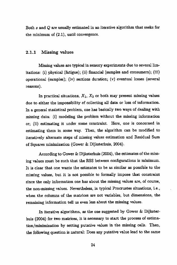
FIGURE 4: Scheme of the distances (RSS) between X\ (before rotation)and the unknown full data X2 and the possible arbitrary configurations*2 »(* = 1> 2,3,4,...) according to the putative values chosen.
For instance, let X2 present some missing values. There is an infinity
of ways of filling its missing cells with putative values, therefore, an infinity
of different initial configurations JJQ (* = 1,2, ), most of them likely
different from the unknown (full) configuration X2 (Figure 4).
Summarizing, three information sources are used to estimate the
missing cells: (i) the information contained in the non-missing data; (ii)
the imposed constraint and; (iii) the information brought in by the putative
starting values. The first one tends to be the weakest; the second tends to
be the strongest; and the levei of interference of the the third is not well
known and is going to be investigated in this paper.
With real and simulated data, we observe the behaviour of the es
timation algorithm for two matrices described by Gower & Dijksterhuis
(2004) imposing the constraint that minimizes the RSS. Simulating differ
ent leveis of loss for non-error and real sized error data sets, we seek for the
25
best way of establishing putative values to start the iterative process.
2.1.2 Methodology
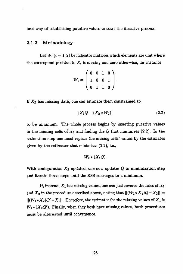
Let Wi (i = 1,2) be indicator matrices which elements are unit where
the correspond position in Xi is missing and zero otherwise, for instance
^0010
Wi = 10 0 1
^0110
If X2 has missing data, one can estimate them constrained to
\\XlQ-(X2*W2)\\ (2.2)
to be minimum. The whole process begins by inserting putative values
in the missing cells of X2 and finding the Q that minimizes (2.2). In the
estimation step one must replace the missing cells' values by the estimates
given by the estimator that minimizes (2.2), i.e.,
W2* (XiQ).
With configuration X2 updated, one now updates Q in minimization step
and iterate those steps until the RSS converges to a minimum.
If, instead, X\ has missing values, one can just reverse the roles of X\
and X2 in the procedure described above, noting that ||(Wi *X\)Q —X2\\ =
11 (Wi*X2)Qf—X\11. Therefore, the estimator for the missing values of X\ is
W\* (X2Q')- Finally, when they both have missing values, both procedures
must be alternated until convergence.
26
Simulation study
For testing the behaviour of such procedures according to the num
ber of missing values, it was considered matrices X\ and X2 (6 x 3) in
situations of perfect match (error-free) and plausible sized error (using em-
pirical data). It was simulated the loss of 5%, 10%, 25% and 50% of the
data in each Xi (i —1,2) and 24 combinations of them (Table 3). Those
combinations correspond to lose 3%, 6%, 8%, 11%, 14%, 17%, 19%, 25%,
28%, 31%, 39%, and 50% of the whole information. Each single combina
tion was repeated 500 times. Of course, the combination of no loss in both
matrices was the full data situation, used as a reference.
TABLE 3: Simulated loss in X\, X2 and in both matrices, expressed as apercentage of the cells.
Loss in Xi Loss in x2 Loss in the whole system5% 0% 3%
10% 0% 6%
25% 0% 14%
50% 0% 25%
5% 5% 6%
10% 5% 8%
50% 50% 50%
For the error-free situation, one fixed matrix X\ was rotated by a
random orthogonal matrix Q for generating the target X2. For the plausible
error situation, one empirical data set was used (Lele & Richtsmeier, 2001),
who measured six landmarks on nine Macqaque skulls.
In order to check the influence of different putative starting values
in the missing cells, three sources were considered: Gaussian and Uniform
distributions and a fixed scalar.
27
Gaussian distributions were defined byparameters \ic and u\, where
fic represents the average of the non-missing cells in one column. Then, one
distribution was used to draw values for each column that presented missing
cells. When a whole column was missing, \ic was set to zero. Parameter a\represents the variance in column c. When the whole column was missing,
a\ was set to one. Note that this procedure is repeated along ali columns
that contain missing cells both in X\ and X2.
Uniform distributions were defined by parameters ac and bc. The
lower and upper limitsac —-acV3 and bc = crc\/3, were ac is the standard
deviation of column c, of course, when c contains missing cells.
The scalar value was set to be zero because ali configurations were
centered before the algorithm to begin. Then, zero was aiways the mean of
every column.
It is clear that when one inserts a putative value coming from a
distribution instead of a fixed mean value, he/she is inserting variability
in the process. However, if the algorithm leads to a global minimum, ali
answers should be the same. Of course, where the putative values are more
far away from the mean, it is expected the convergence to happen after a
higher number of iterations.
The behaviour of the estimates was evaluated along ali situations,
namely, the combinations of two types of error size: non-error (perfect
match) and real sized error (empirical data set); three sources of putative
values: Gaussian distribution, Uniform distribution and scalar zero; and
ali leveis of induced loss. To check the behaviour of the estimates five
parameters were examined, u, <5, <f>, rj andR2. Their meanand the standard
deviation were recorded along 500 replications.
28

(a) Residual Sum of Squares discrepancy (u):
u = RSS - RSSe,
where RSS is the Residual Sum of Squares after adjustment of the full
data sets and RSSe is the Residual Sum of Squares after match the
data sets under loss and posterior estimation.
That parameter u indicates how similar the estimated data sets are
from the full data sets in terms of match. It is one of the possible
Índices of quality of estimation. The closer to zero u> is, the similar are
the RSS's. However, it is worth noting that is expected the RSSe to
be smaller than RSS since the estimation constraint imposes that the
estimates are such that the RRS is minimum.
(b) Mean squared loss (õ):
E2., *£,(*£-#)*í =
77li + ?7l2
where m, is the number of missing values in Xi (i = 1,2); xff is thereal value of the jth missing cell in Xi (j = 1,... ,mi); and xfj is itsestimate.
That is a really quality of estimation index. It achieves the mean
quadratic distance between the real value and the estimate of a missing
cell, along ali of them. Clearly, the smaller is õ, the better are the
estimates.
(c) Scaling factor discrepancy (<f>):
4> = S —$e,
where s is the scaling factor obtained when one matches the full data
sets and se is the scaling factor when the sets have estimates in their
missing positions.
29
Of course, one wants se to be as similar as possible to s, but the be
haviour of <j> along an increasing number of missing values is not trivial.
(d) Number of iterations until convergence (77).
That parameter indicates efficiency. Besides achieve the right answer
(the global minimum of the function), one wants to do that as fast as
possible. Though, one wants n to be small.
(e) Explained variation (R2)
R2 =2_ Var(fitted) _ 2síroce(E)
Var(Total) s2||Xi|| + ||X2|r
In this case, R2 suggests how similar X\ transformed can be to X2.
Again, this parameter indicates quality of match. The closer to one,
the better the match.
AH computations were performed by specifically made R functions
(Appendix B).
2.1.3 Results and discussion
Results were divided into two sections: (a) Exact match and (b)
Real sized error. Here, is explored the behaviour of each parameter along
the increasing value of missing cells in the whole system. It could be ex
plored the behaviour along missing cells in just one matrix, but it would
be redundant, since they were quite similar.
2.1.3.1 Exact match
In this situations there is no error, since X2 is a perfect transforma
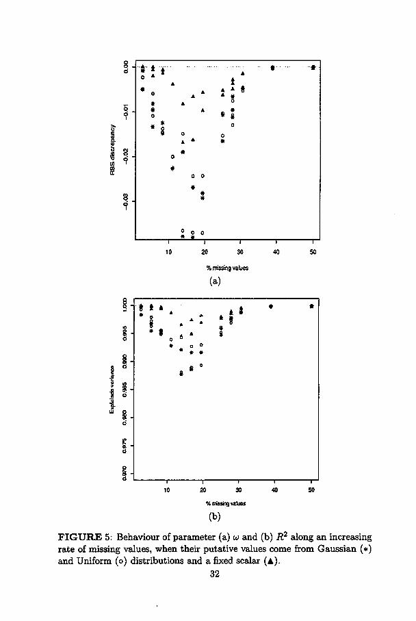
tion of X\. According to Figure 5a one notes that the discrepancy between
RSS of full data sets and estimated data sets is small with few or too many
30

missing values. That is easy to understand since when one has few missing
values, the situations are very similar; and when one has too many ones,
their estimates are such that the RSS is minimum. Since the original RSS
is already zero (perfect match), then the discrepancy tends to decrease.
A similar behaviour is observed in R2 (Figure 5b). With the same
explanation given above one can understand why R2 is maximum in cases
of few and too many missing values.
For both u and R2 the best behaviour were given by the putative
values set to zero. In fact, if one constructs confidence intervals based on
Normal distribution for those parameters one can note that the estimates
do not differ statistically from source to source, but, since setting a fixed
scalar is very much easier than sampling from a distribution, there is no
reason to consider the most complicated options.
In Figure 6a, one can observe that 6 is much smaller when the scalar
zero is used. Again, the worst situation happens in a median rate of loss.
The estimates of n are more similar along putative sources, but the worst
behaviour happens in the same percentage of missing values.
It is worth remembering that the apparent straightforward estima
tion when there are too many missing values is not a good thing, since
the estimates are necessarily similar to the missing data. They are just
convenient to turn the matrices similar and the match better.
Scaling factor discrepancy <j> brings us a more fare result in Figure 7.
The more missing values, the worst the scaling factor that results from the
matching. That is a strong argument against the apparent good situation
of having several missing values.
31
*
%missing values
(a)
% missing values
(b)
FIGURE 5: Behaviour of parameter (a) u and (b) R2 alongan increasingrate of missing values, when their putative values come from Gaussian (*)and Uniform (o) distributions and a fixed scalar (a).
32
8 .I I
i I
8 -
% missingvalues
(a)
20 30
% rntssinQ values
(b)
FIGURE 6: Behaviour of parameter (a) õ and (b) 77 along an increasingrate of missing values, when their putative values come from Gaussian (*)and Uniform (o) distributions and a fixed scalar (a).
33
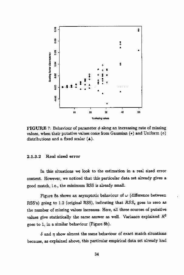
FIGURE 7: Behaviour of parameter <f> along an increasing rate of missingvalues, when their putative values comefrom Gaussian (*) and Uniform (o)distributions and a fixed scalar (a).
2.1.3.2 Real sized error
In this situations we look to the estimation in a real sized error
context. However, we noticed that this particular data set already gives a
good match, i.e., the minimum RSS is already small.
Figure 8a shows an asymptotic behaviour of u (difference between
RSS's) going to 1.2 (original RSS), indicating that RSSe goes to zero as
the number of missing values increases. Here, ali three sources of putative
values give statistically the same answer as well. Variance explained R2goes to 1, in a similar behaviour (Figure 8b).
6 and 77 show almost the same behaviour of exact match situations
because, as explained above, this particular empirical data set already had
34

«N _
% missingvalues
(a)
20 30
% missingvalues
(b)
FIGURE 8: Behaviour of parameter (a) u and (b) R2 along an increasingrate of missing values, when their putative values come from Gaussian (*)and Uniform (o) distributions and a fixed scalar (A).
35
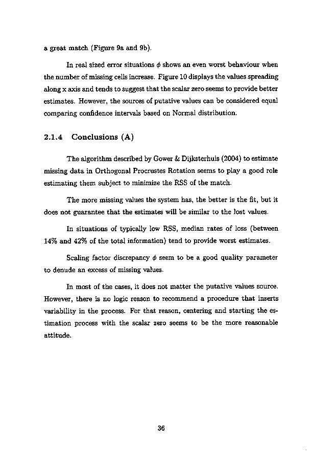
a great match (Figure 9a and 9b).
In real sized error situations <f> shows an even worst behaviour when
the number of missing cells increase. Figure 10 displays the values spreading
along x axis and tends to suggest that the scalar zero seems to provide better
estimates. However, the sources of putative values can be considered equal
comparing confidence intervals based on Normal distribution.
2.1.4 Conclusions (A)
The algorithm described by Gower& Dijksterhuis (2004) to estimate
missing data in Orthogonal Procrustes Rotation seems to play a good role
estimating them subject to minimize the RSS of the match.
The more missing values the system has, the better is the fit, but it
does not guarantee that the estimates will be similar to the lost values.
In situations of typically low RSS, median rates of loss (between
14% and 42% of the total information) tend to provide worst estimates.
Scaling factor discrepancy $ seem to be a good quality parameter
to denude an excess of missing values.
In most of the cases, it does not matter the putative values source.
However, there is no logic reason to recommend a procedure that inserts
variability in the process. For that reason, centering and starting the es
timation process with the scalar zero seems to be the more reasonable
attitude.
36

% missingvalues
(b)
FIGURE 9: Behaviour of parameter (a) 6 and (b) 77 along an increasingrate of missing values, when their putative values come from Gaussian (*)and Uniform (o) distributions and a fixed scalar (a).
37
& <s
FIGURE 10: Behaviour of parameter <f> along an increasing rate of missingvalues, when their putative values come from Gaussian (*) and Uniform (o)distributions and a fixed scalar (A).
2.2 Generalised Procrustes Analysis (GPA)
Until 1975, Procrustes problems used to concern only with two data
sets, that is, when one matrix is transformed to match one target. In that
year, Gower generalised those problems to deal with k sets. In nowadays,
many practical applications demand matching more than two configura
tions. To state a notation, consider the following Procrustes problem1
f(s\,..., Sfc,«i,..., Ufc,7i,...,Tk) =k
=53 \\sí(Xí - lu'i)Ti - Si^Xv - ItijOIVIl, (2.3)
1Although in general transformations the scaling factor (s») becomes meaningless,since it is absorbed by the matrix Ti (i = 1,... ,£), here the most general problem isstated and ali estimators derived in order to promptly obtain any particular case latter.
38
where Xi is a known nxp data matrix; Si is a scaling factor; Ui is a
translation vector; and Ti is a general transformation matrix (i < i' —
1,...,*).
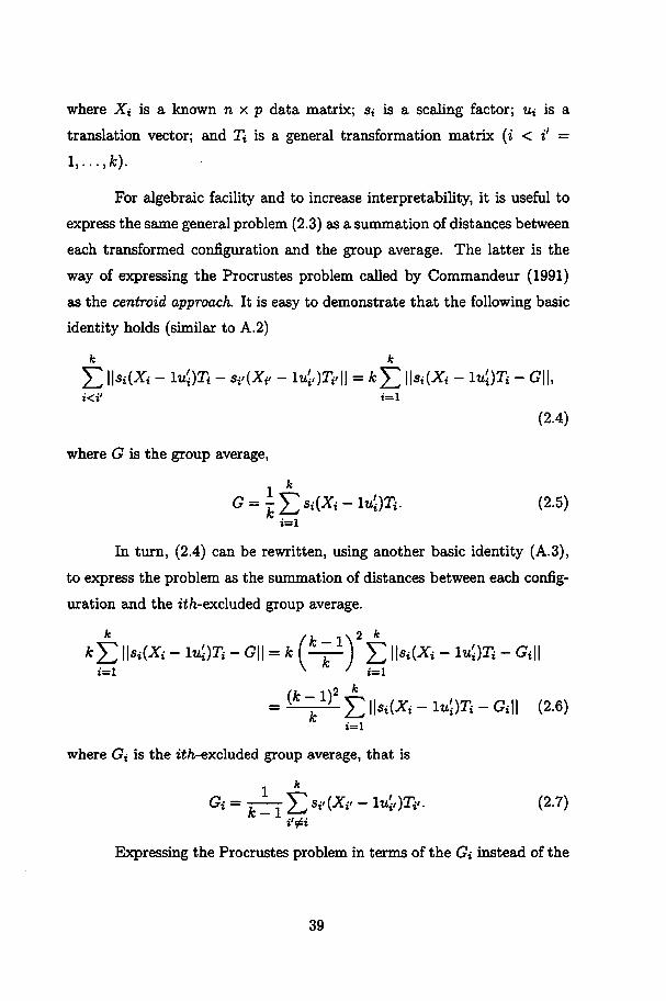
For algebraic facility and to increase interpretability, it is useful to
express the same general problem (2.3) as a summation of distances between
each transformed configuration and the group average. The latter is the
way of expressing the Procrustes problem called by Commandeur (1991)
as the centroid approach. It is easy to demonstrate that the foUowing basic
identity holds (similar to A.2)
k k
J2 \\sí(Xí - lu^Ti - 8i'{Xe - luíOZVII =*£ \\sí(Xí - ltií)T« - G||,i<i' i=l
(2.4)
where G is the group average,
1 kG=-^^(Xi-lOTi. (2.5)
In turn, (2.4) can be rewritten, using another basic identity (A.3),
to express the problem as the summation of distances between each config
uration and the iíh-excluded group average.
kf^ \\sí(Xí - lvl)Ti -G\\ =k(±Z1) £ \\Si(Xi - ltQTi - Gi\\t=i \ ft / i=1
where G% is the ií/i-excluded group average, that is
1 kGt =y^ £ MXi> - 1«Í0^. (2.7)
Expressing the Procrustes problem in terms of the Gi instead of the
39
commonly used G, one observes two advantages: (i) it avoids the patholog-
ical case where the group average is zero; and (ii) the ií/i-excluded group
average does not depend on Xá, what helps improving the efficiency of the
estimation algorithm.
For notation facility, let Xã denote the ith centered configuration,
i.e. Xd = Xi—lUi- Moreover, from nowon lets suppress the constant ~k
from (2.6) since it is imaterial for the minimization process. Therefore, (2.6)
becomesk
YtWsiXciTi-GiW. (2.8)t=i
2.2.1 Considerations about non-orthogonal GPA
Considering non-orthogonal transformation matrices Ti for post-
multiplying data matrices Xi in Procrustes problems is a quite old and
not so developed issue. It might be so because of the good properties of or-
thogonal matrices Q*. They are able to simplify a great deal of the álgebra
and allow prompt practical interpretations. Moreover, they preserve the
relative distances between vértices of the configurations, i.e. they promote
rigid body rotations and preserve the original classification done by the
assessor.
However, some effort must be done towards finding and interpreting
non-orthogonal transformations able to minimize Procrustes problems (by
the way, to lower minima than orthogonal ones), under a suitable constraint.
Moreover, orthogonal transformations (Qi) are a particular case of general
transformations (Ti). Thus, since the álgebra is well known for Ti it is
immediately known for Qi, in a simplified form. Algorithms as well, can be
proposed for allowing the more general case and then computer packages
can allow the user to choose the desired transformation according to his/her
practical needs.
40
Particularly, Gower & Dijksterhuis (2004) are concerned in devel-
oping a lot of álgebra involving general transformations Ti. A tiny part of
them is rewritten here.
Following, some álgebra is developed and some is reported for or
thogonal and non-orthogonal cases, along the estimation of missing values,
transformation matrices, scaling factors and translation vectors.
2.2.2 General transformation
(a) Estimating missing values
First of ali, lets describe an estimation process of missing values
suggested by Gower & Dijksterhuis (2004). It is a modified EM (estima-
tion/minimization) procedure that seeks for those estimates of missing val
ues that minimize a least squares metric. That procedure is described using
the notation adopted here rather than the notation used by the authors.
The following describes the estimation procedure for the ith X matrix and,
of course, the same process must be repeated for every matrix X that have
missing values.
Suppose Xi has M values missing in cells (ii, ji), (Í2> J2), •••>(ím,3m)-
The missing values may be estimated by a variant of the iterative EM al-
gorithm (Dempster et ai., 1977) where "M", rather than representing a
step for maximum likelihood estimation, now stands for the least-squares
Procrustes minimization, while "E" is a step, described below, that gives
expected values for the missing cells.
For fixed TV (i' = 1,..., k) and X? {%' # i) the terms of £?«/ \\XíTí-XíiTí'|| that involve Xi requires the minimization of the criterion \\XíTí —
Gi\\ over the unknown values in given cells (iuji),(Í2J2),-••,(ímJm)-
Recall that Gi represents the ií/i-excluded group average, which is inde-
41

pendent of Xi. One assumes that the cells with unknown values contain
putative values that one seeks to update by minimizing the criterion. Sup-
pose even that the updates are given in a matrix Xui, which is zero except
for the missing cells which contam values denoted by xi, x2,..., xm- Thus,
one wishes values of XUi that minimize2:
\\(Xi - Xui)Ti - Gt\\ = \\XuiTi - (XíTí - Gi)\\. (2.9)
This is a Procrustes problem itself, where now it is XUi, rather than
Ti, that is to be estimated. Transposition would put (2.9) into the basic
form. The constraint on XUi may be written:
M
Xui = xiehe'h +x2ei2e'j2 + ...+ xMeÍMe'JM = ^ Xmeime'jm (2.10)171=1
where, as usual, ei represents a unit vector, zero except for its ith position.
This function is linear in the parameters xm so, in principie, the minimiza
tion of (2.9) is a simple linear least-squares problem; unfortunately, the
detailed formulae are somewhat inelegant (A.5). The terms in (2.9) that
involve Xui ara
tr[(XuiXUi)(TiTl) - 2Xuí{XíTí - G<)3Í] (2.11)
which one writes:
tr[(XuiXui)T-2XuiY} (2.12)
where T = TiT? issymmetric andY = {XíTí-Gí)TÍ, is the current residual
matrix.
The minimization of (2.12) over one missing cell xr, r = 1,2,..., M,
2(2.9) is demonstrated in (A.4).
42
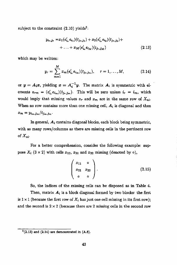
subject to the constraint (2.10) yields3:
Virjr =a;i(eireii)(<ir,ii) + x2{eirei2){tjrij2)+
+ -.. + xM(e'ireÍM)(tjr,JM) (2.13)
which may be written:
M
Vr = Y^ xm(eleim){tjr,jm), r= 1,..., M, (2.14)m=l
or y = AiX, yielding x = A^xy. The matrix Ai is symmetric with el-ements a™ = (eípeim)(íjr,jm)- This will be zero unless iT = im, whichwould imply that missing values xr and xm are in the same row of XUi.
When no row contains more than one missing cell, Ai is diagonal and then
Xm = yim,jm/tjm,jm'
In general, Ai contains diagonal blocks, each block being symmetric,
with as many rows/columns as there are missing cells in the pertinent row
of Xui.
For a better comprehension, consider the following example: sup-
pose Xi (3 x 2) with cells xn, £31 and X32 missing (denoted by o),
' £11 o 1
X21 Z22 • (2.15)
\ o o )So, the Índices of the missing cells can be disposed as in Table 4.
Then, matrix Ai is a block diagonal formed by two blocks: the first
is 1 x 1 (because the first row of Xi has just one cell missing in its first row);
and the second is 2 x 2 (because there are 2 missing cells in the second row
l(2.13) and (2.14) are demonstrated in (A.8).
43
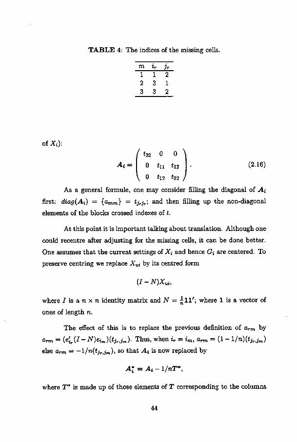
TABLE 4: The Índices of the missing cells.
m ir jr1 1 2
2 3 1
3 3 2
ofXi):
f <22 0 0 ^*i= 0 in íia • (2.16)
\ 0 tu *22 /
As a general formule, one may consider filling the diagonal of Ai
first: diag(Ai) = {%«} = fyrJ-r; ^d tnen filling up the non-diagonal
elements of the blocks crossed indexes of í.
At this point it is important talking about translation. Although one
could recentre after adjusting for the missing cells, it can be done better.
One assumes that the current settings of Xi and hence Gi are centered. To
preserve centring we replace Xui by its centred form
(I-N)Xui,
where íisanxn identity matrix and N = £ll'; where 1 is a vector ofones of length n.
The effect of this is to replace the previous definition of Orm by
Orm = (el(I- N)eim){tjrjm). Thus, when ir = im, a™ = (1 - l/n)(tjrjm)else Orm = —l/n(tjrjm), so that Ai is now replaced by
At = Ai-l/nT*,
where T* is made up of those elements of T corresponding to the columns
44
of the missing cells (e.g. the third column of Table 4):
and when T is symmetric, tjrjm = tjmjr.
In the example, assume T* is a tabular form to turn explicit the
Índices r and m:
m/r 1 2 3
1 / *22 Í12 *22 *
2 Í21 íll <12
3 \ Í22 Í12 <22 /
This minor change gives x = A*~1y, so defining Xui, and then{In)Xuí gives the required correction matrix. This is ali that is necessary
for handling translations. Recentring XUi derived from x = A~^xy andusing (I-N)Xui derived from x = A*~xy will give different updates to themissing values, though both must converge to the same final estimates. A
near exception to this rule occurs for orthogonal transformations when the
two approaches hardly differ (Gower & Dijksterhuis, 2004, Section 9.2.1).
Now, an alternative procedure is presented for finding estimates of
the missing values. Such procedure intends to be an easier and compu-
tationally lighter alternative to the one described above. However it is
based on the same principie, that is, finding those estimates that minimize
a residual sum of squares. The main difference is the way the problem of
Procrustes is stated.
Suppose the following Procrustes problem, in a least squares metric:
k
Yl \MXa + Wi*Xui)Ti - Gi\\, (2.17)<=i
where Xá has putative values in unknown cells (say, zeros); Wi is an in-
dicator matrix that contains ones in unknown cells addresses and zeros
45
otherwise; Xui is an update matrix for Xi\ and * stands for an element-
wise product. Now, for notation matters, let X^ = Wi * XUi, where the
upper index r stands for restricted.
At this point a remark is necessary: when considering general trans
formations Ti it is not necessary to consider scaling factors Si. The effect
of the scafing factors is absorbed by the Ti's. However, one intends to state
the problem on its more general form, for which orthogonal rotation Qi is
a special case. In turn, when orthogonal rotation Qi is allowed, the use of
Si does make sense.
If one consider ali parameters known but the update matrix X^, for
each i = 1,..., k, one has to minimize
WsiiXá + X^Ti-Gill
what is the same as minimizing4:
tr[(x£Xà)T-2X£n (2.18)
where T = TOi and Y = (s~lGi - X^T!.
Minimizing (2.18) over X^ leads to the least squares estimator5:
Xrui = YT~1 (i = l,...,fc). (2.19)
However X^ is not necessarily restricted, that is, nothing guarantees
it has only values in the missing addresses and zeros otherwise, but as the
estimation process is already iterative, it possibly tends to converge to a
restrict matrix as is desired. Therefore, for obtaining estimates specifically
4Proof is given in (A.10).5Demonstration is given in (A.9).
46
for the missing values, one can restrict the answer:
Xrui = YT-1
W~7xui = YT-1
W^7Xui = Wi*YT-1.
Accordingly to the prior procedure described here, the translation
correction can be insert as well. Derivation of the estimator is omitted, but
it is similar:
Xli = Wi *[(/ - N^YT-1}. (2.20)
where [I-N) is as defined above. Howeveris important noting that (I—N)
can require generalised inverse due to possible singularity.
Of course such procedure is not so elegant as Gower & Dijksterhuis'
but it is a (at first sight) easier and computationally Hghter alternative that
might lead to the same answer when it converges.
(b) Estimating transformation matrices
Deriving the estimator of transformation matrices T» depends on the
constraint inserted into the minimization process.
With no restriction, i.e. deriving the estimator without any kind
of constraint, estimating Ti is solving a multivariate multiple regression
problem. In problem (2.8), considering s^ Xà and Gi as fixed6, it is easy
to solve the multivariate multiple regression problem7:
ti = -(XUXa^XUGi. (2.21)Si
However, some kind of constraint is suitable for avoiding trivial so-
6Remember that XCi is not usually fixed because it is function of Xui; and Gi isfunction of 7V, for i' -^ i, considered fixed by the algorithm when estimating T».
rDemonstration in (A.11).
47
lutions as Ti = ... = Tfc = 0, where 0 is a matrix (p x p) of zeros.
Gower & Dijksterhuis (2004) derive an estimator of Ti minimizing a
Procrustes problem under a general quadratic restriction. That derivation
follows.
Consider the Procrustes problem rewritten in a hypermatrix form:
k
S= Y, WXciTi - XrfZVH = tr(kV'AV - V'ZV), (2.22)
where Z = {X^X^}, A = diag{X,clXcl,X'<âXc2,...,X'ckXck) and V =
T[,T'2,..., Tfk. Now, consider the constraint in a general form:
diag{aV'AV + (3V'ZV) = I, (2.23)
which can turn into severa! constraints. For instance, setting a = l/k and
0 = 0 generates the constraint diag{V'AV) = kl\ and setting a = 0 and
(3 = l/k2 gives diag{V'ZV) = k2I = fc2G'G. Differentiation of (2.22) with
Lagrange multipliers 7ii72> •••»7fl> axí^ writing T = dzap(7i,72,... ,7J?)>
gives:
fcAF - ZV = (aAF + 0ZV)T. (2.24)
Pre-multiplying the above by V and using (2.22) and (2.23), imme
diately shows that S = tr(F), so the criterion is minimized by selecting the
R smallest values of 7r that satisfy (2.24). One may rewrite (2.24):
ZV = AV$, (2.25)
where * = (kI-áT)(I+0T)'-1. Asusual, the matricesVZV and V'AVare
diagonal. Thus one has orthogonality even though (2.23) only constrains
the diagonal elements of these matrices. Thus (2.23) becomes:
ocV'AV + /3V'ZV = I,
48
which in combination with (2.25) gives the scaling of the columns of TV
[V'AV){aI+ 0*) = {V'ZV){a$-1 + 01) = /.
However a two-sided eigenvalue problem requires at least one of the
given matrices in (2.25), (Z or A) to be positive definite, and since Z and
A are formed by X'uiXui they are both typically positive semi definite.
For that reason, the determination of Ti, that is V, is not straightforward.
Therefore, the further works are needed for developing Procrustes problems
with general transformations Ti.
(c) Estimating scaling factors
It is worth noting that, in the general transformation case, the scal
ing factors become meaningless since they are absorbed by the matrices Ti
(i = 1,..., k). However, if, for some reason, they need to be estimated in a
general case, it would be possible. Moreover, its estimator will be derived
here for didactic reasons, namely, the estimation process of scaling factors
in the orthogonal case will be showed to be a particular case of this one.
First of ali, lets rewrite (2.3) allowing for missing values as in (2.17)
but with Xi already centered as in (2.8).
k
f(si, ...,**) = £ WsiiXa +WitXuiW-SirlXcP +Wi,*XUi>)Ti,\\ (2.26)t<t'
To simplify the notation, one can let Xà + Wi * XUi = X^, i.e.
configurations centered and enabled for missing data. That yields
k
/(«i, ...,«*) = £ WsiXSTt - s^X^Ti^W. (2.27)
Moreover, at the scaling factor step, one must consider the other
variables to be fixed, namely Xtí and Ti. Therefore, (2.26) and (2.27) turn
49

out into functions of Si.
Rewriting equation (2.27) in a matrix form8, gives
/(«i,..., sk) = k[s'diag{S)s) - s'Ss (2.28)
where s is a vector containing ali Si and S is a symmetric matrix with
elements Sü' = {tr{T!X£X^T!)}, i = l,...,k.
Note that minimizing the loss function (2.28) is maximizing
h{s) = s'Ss. (2.29)
In order to avoid the trivial solution s\ — s2 = • • • = sjt = 0,
one must consider a suitable restriction. Suppose one imposes that the
configurations must have the same total size before and after the scaHng
transformation, i.e.,
k k
Dl^TiH = D|5íX-Tí||. (2-3°)t=l i=l
Gower & Dijksterhuis (2004) emphasize that the scaled configuration
is important to be set to a fixed value, what is respected assuming X^ and
Ti to be fixed at this estimation step.
Expressing (2.30) in matrix notation using the prior definition of s
and S and assuming diag(S) to be a diagonal matrix corresponding to the
main diagonal of S, gives
tr{diag{S)) = s'diag{S)s. (2.31)
Since diag(S)z diag(S)~2 = Ik, where Ik is a k dimensional identity,
(2.29) can be rewritten as
h(s) = s'diag{S)*diag{S)-* S diag(S)~*diag{S)2 s.
8Proof is given in (A.12).
50
Now, let
diag(S)~* S diag(S)~* = P$P'
be an eigenvalue-eigenvector decomposition, where P is a (kxk) orthogo
nal matrix containing the eigenvectors and $ is a (k x k) diagonal matrix
containing the eigenvalues of diag(S)~* S diag(S)~2. Then, the
expression (2.29), to be maximized, can be expressed as
h(s) = s'diag(S)2 P$P'diag(S)% s.
Now, if one let a = P'diag(S)z$, then
h(s) = a'$a.
Since
h(s) = a'$a < (f>ia'a,
where <f>\ is the largest eigenvalue and
a'a = s'diag(S)~2 PP' diag(S)z s
= s' diag(S)s
= tr(diag(S)),
then,
h(s) = a'$a< (f>itr(diag (S)). (2.32)
Since one wants to maximize a'<è a, one seeks for s such that h(s) =
<f>itr(diag(S)).
Lets denote pi the eigenvector associated with the largest eigenvalue
51
<f>i, then rewriting (2.32) in the form of (2.29), gives
h(s) = <j>\tr(diag (S))
= tr(diag (S)) p'lP$P'pi
= (tr(diag(S))2diag(S)~2pi) S (tr(diag(S))2diag(S)~ipi\=h(tr(diag (S))*diag(S)-*pi) .
So, the estimator of s should be
s = tr(diag (S))5 diag(S)~bpi, (2.33)
since it minimizes the loss function (2.28) and satisfies the constraint (2.31),
s,diag(S)s = (tr(diagS)2diag(S)~^p\J diag(S) Ur(diagS)2diag(S)~2piJ
= tr(diag(S))p[diag(S)~2diag(S) diag(S)*pi
= tr(diag(S))p'1p\
= tr(diag(S)).
(d) Estimating translation vectors
An easy way of dealing with translation vectors Ui (i — \,...,k)
is performing the estimation/minimization algorithm concerning only with
Xà, i-e-» centering the X matrices at each step. After convergence, the
translation vectors Ui can be estimated by the average of the columns of
Wi * Xi —Xâ and then, the estimator of the translation matrix is
lüí. (2.34)
52
2.2.3 Orthogonal transformation
When the transformation matrices Ti (i —1,..., k) are restricted to
be orthogonal (say, Qi), the expressions tend to become simpler due to the
general properties of the orthogonal matrices.
(a) Estimating missing values
In the procedure described by Gower k Dijksterhuis (2004), making
Ti = Qi turn things simpler. When no correction for translation is done in
the missing cells, the estimator x = A~*y simplifies for x = y. However,
when the translation correction is done, the estimator of missing cells re-
mains x = A*~1y, because though T = A = Ip, T* and consequently A*are not identities necessarily.
In the procedure proposed here, the estimator expression for X^ do
becomesimpler as well because T reduces for identity (T = QíQí = Ip) and
Y reduces for GiQJ —SiXà-
Therefore, the new estimator for X^{ (i = 1,..., k) is
Xrui = Y = GiQ'i-siXci (2.35)
or
Ki = Wi * [(/ - AO-HGzQÍ - SiXâ)}, (2.36)
when translation correction is allowed.
(b) Estimating rotation matrices
When one wants Tf to be orthogonal, producing a rigid body rotation
in Xà, the solution is well known.
53
Consider (2.17) setting Ti = Qi, then
k
J2 WsiXàQi - Gi\\ =tr {s2Q'iX<XàQi - 2^*^ - G{Gi)
=tr (s2XÍXà ~2siG'iXàQi - Gfii) . (2.37)
Since Gi does not depend on Qi, and remembering that Si and XÜ
are considered to be fixed at this step, minimizing (2.37) is maximizing
tr(G'iXàQi)- Remember that one wants Qi to lead the function above to
its minimum and to be orthogonal. Then, for i = 1,..., k, expressing<2JX^
in terms of its singular value decomposition G^X^ = t/iEil^', where U and
V are orthogonal matrices and E is diagonal, gives
tr {G^Qi) = tr (UíEíV/Qí)
tr(G'iXàQi)=tr(XiV{QiUi)
= tr (XíHí) ,
where Hi = V(QíUí, being the product of orthogonal matrices, is itself
ortogonal. Considering the elements of Si and Hi, respectively, Ei = aj
and Hi = %, one has that
p
ír(Eiiíi) = 22h35Ghi=i
which, because the singular values <73 are non-negative, is maximum when
hjj = 1 for j = 1,... ,p, the maximal value attained by the elements of an
ortogonal matrix. Thus at the maximum Hi = I giving, I = V!QíUí and
Qi = ViUi
Therefore, the estimator Qi that minimizes the Procrustes problem
and guarantees Qi to be orthogonal is:
Qi = VU' i = l,...,A:. (2.38)
54

(c) Estimating scaling factors
Scaling factors are obtained from the same standard eigenvalue prob
lem (2.33), but its argument matrix is modified,
s = tr(diag (A))* diag(A)~%pi, (2.39)
where A is slightly different from S, i.e., it is function only of the centered
configurations Aa> = {tr{X^X^,)}.
(d) Estimating translation vectors
Following the same principie of centering Xi in each step of the al
gorithm and estimating Ui at the end, the estimator üi remains the same
(2.34) if one is performing an orthogonal transformation in the configura
tions.
2.2.4 Algorithm
Empirical tests have shown that the order of the steps in the modi
fied EM algorithm is responsible for a slower or faster converge. Moreover,
estimating ali parameters within each i or, for estimating within each pa-
rameter alU = 1,..., k, also seems to make a great effect. However, further
works must be done to comprove and explain such phenomenon. Following
algorithm is already in the suggested order:
1. Insert putative values in the missing cells of matrices XUi and computeXi, %= 1,..., k.
2. Centre matrices X* obtaining Xtí, i = 1,..., k.
3. Normalize X^, i = l,...,k.
4. Set initial matrices Ti to identities and s to unit vectors.
55
5. Compute the ií/i-excluded configurations Gi, i— l,...,k.
6. Compute the initial residual sum of squares (Procrustes loss).
7. Estimate updated transformation matrices Ti or Qi, i = 1,..., k.
8. Estimate the missing values and update X^, i —1,..., k.
9. Recentre X^, i = 1,..., k.
10. Update Gi, i = 1,..., k.
11. Estimate new scaling factors Si, i = 1,..., k.
12. Recompute the Procrustes loss and compare with its previous value.If their different suits a desired converge tolerance, than the processis finished. Otherwise, return to step 7.
2.2.5 Conclusions (B)
Algorithms for estimating missing data in Procrustes problems are
still a unfinished field although well discussed in the recent literature. De-
termining a suitable (optimum) algorithm (order of steps) is a field to be
explored.
On the other hand other constraints should be investigated in order
to provide estimates closer to reality, i.e., closer to the cells that are missing.
For non-ortogonal transformations, two-sided eigenvalue problems
with both matrices positive semi-definite must be solved in order to guar-
antee such the convergence of the estimation process to plausible values.
Moreover, practical interpretation of such transformations are still waited
for a closer relation with sensory experiments.
56
3 STATISTICAL INFERENCE AND GPA
3.1 Introduction
Generalised Procrustes analysis (GPA) is considered a descriptive
multivariate statistical method (Ferreira, 2004). A graphical method that
allows relative statements concerning a set of objects in its answer-plan.
Therefore, one of the results of GPA is an answer plan containing the two
first dimensions of maximal variation. When G is referred to that plan,
its n points (n objects) represent the consensus configuration. In sensory
analysis it represents the 'mean' scores, along the assessors, to ali analyzed
objects. However, each assessor configuration can be referred as well, for
instance, to check their distance from the group average. That plan is
generated by two axes that represent linear combinations of the attributes
(dimensions) used to describe the objets.1
However, GPA presents some Ümitations. Though any assumption
is necessary to be made about the multivariate distribution of the scores
given to objects' attributes, the current methodology does not allow the
statistical inference about a population of possible consumers of a product,
for instance. In other words, there is no statistical inference in Procrustes
analysis. It does not allow neither an interval estimation of the position of
an object in a multivariate sensorial space nor hypothesis tests with a levei
*It is worth noting that the number ofprincipal axes investigated may vary from 1 top, though it is most common to restrict the inference to the first two axes (the plan).
57

of significance associated. The only possible conclusions are relative ones.
i2 CM -
I
-4
Principal Axis 1
(a)
,G
o -
CM -
t- - ?
,E
7 _
CM _1 D'
1 i 1 1 1
-2 -1
Principal Axis1
(b)
FIGURE 11: (a) Relative eucUdian distances between objects A, B e C(b) EucUdian distances between objects D and E.
58
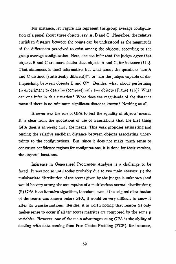
For instance, let Figure lia represent the .group average configura
tion of a panei about three objects, say, A, B and C. Therefore, the relative
eucUdian distance between the points can be understood as the magnitude
of the differences perceived to exist among the objects, according to the
group average configuration. Here, one can infer that the judges agree that
objects B and C are more similar than objects A and C, for instance (lia).
That statement is itself informative, but what about the question: "are A
and C distinct (statistically different)?", or "are the judges capable of dis-
tinguishing between objects B and C?". Besides, what about performing
an experiment to describe (compare) only two objects (Figure 11b)? What
can one infer in this situation? What does the magnitude of the distance
mean if there is no minimum significant distance known? Nothing at ali.
It never was the role of GPA to test the equality of objects' means.
It is clear from the quotations of use of translations that the first thing
GPA does is throwing away the means. This work proposes estimating and
testing the relative eucUdian distance between objects associating uncer-
tainty to the configurations. But, since it does not make much sense to
construct confidence regions for configurations, it is done for their vértices,
the objects' locations.
Inference in Generalised Procrustes Analysis is a challenge to be
faced. It was not so until today probably due to two main reasons: (i) the
multivariate distribution of the scores given by the judges is unknown (and
would be very strong the assumption of a multivariate normal distribution);
(ii) GPA is an iterative algorithm, therefore, even if the original distribution
of the scores was known before GPA, it would be very difficult to know it
after its transformations. Besides, it is worth noting that reason (i) only
makes sense to occur if ali the scores matrices are composed by the same p
variables. However, one of the main advantages using GPA is the abiUty of
deaUng with data coming from Free Choice Profiling (FCP), for instance,
59
i.e., each matrix can contain its own set of variables. Remember that GPA
is methodology that compares configurations, and those configurations are
formed by dimensions rather than variables.
Therefore, intensive computational techniques are suitable for han-
dling that situation. Here, mainly bootstrap techniques are used to estimate
the empirical distribution of the desired parameters' estimators (whichever
is the original scores distribution). Thus, such a methodology can enrich
GPA's potentialities allowing estimation and decision theories to be stated.
3.2 Sampling in Sensory Sciences
Some discussion was already done in section 1.4, but here one intend
to stress some considerations and address some recommendations.
GeneraUy, statistical tests require a sample to be selected randomly
from the population it represents. This may be a complex matter but there
are additional points of design which are worth mention here.
When sampling, one must select the sample in an unbiased manner.
In practice, a so-caUed random sample is rarely completely random. Sub-
jects are usually volunteers and volunteers are not necessarily representa-
tive of the population from which they were drawn. Also, an experimenteis
method of choosing subjects is hardly ükely to be random; he or she wiU
tend to select those who are friendly and enthusiastic, as well as those who
are conveniently near the testing location. The importance of such difficul-
ties is more a matter of philosophy than mathematics; it is certainly hard to
gauge. Unfortunately, such questions are rarely considered; experimenters
seem to hope that they are unimportant. For instance, one of the common
errors in sensory work with foods is to sample from the wrong population
(0'Mahony, 1985).
60
Further, members of the sample may also teU lies. This can oc-
cur when question of a personal nature (money, sex, etc) are asked. The
tendency to please the experimenter and give the 'right' answer is strong
among human subjects.
Control groups are often used to distinguish what is been estimated
(treatments, blocks, variables, etc) for any from any other effect that might
be happening. The response of non-treated experimental units is the ex-
pression of the so called placebo effect. By comparing treated units and
control a measure can be obtained, independent of any suggestion. Control
groups are often used in behavioral research and could sometimes be useful
in the sensory analysis of foods.
GeneraUsed Procrustes analysis deals with data coming from ex-
perts, trained, semi trained, untrained, consumers, etc. Furthermore, GPA
is sufficiently dynamic to treat scores produced by different scales, contain
ing different sorts of bias; each assessor can use how many and whatever
variables they want to measure the same object. By definition, GPA is not
concerned in comparing means but configurations. GPA adjusts configu
rations and identifies mains agreements and disagreements among judges.
For those reasons, GPA is more important in a Free Choice Profile (FCP)
context (WiUiams & Langron, 1984). For any other, say, 'balanced' situa-
tion, 'classicaT multivariate statistical tools, such as Principal Components
Analysis (PCA), Factor Analysis (FA), Cluster Analysis (CA), Partial Least
Squares Regression (PLSR), Multivariate Analysis of Variance (MANOVA),
etc, tend to be more adequate. Therefore, due to the huge freedom to vary
of FCP, semi trained and untrained assessors can be drawn from correspon-
dent populations, leading that to be a random effect.
61
3.3 Generalised Procrustes Analysis
Lets Xi (i = 1,..., k) be k data matrices, representing A: assessors,
with dimensionality nxp,, where n is the number of evaluated objects (l =
1,..., n) and pi is the number of dimensions or attributes used by assessor
i (j = l,.--,Pi)- In each of those matrices, the Ith row represents the
coordinates of a point S\ in the space Rpi. In a sensory analysis context,it represents the Ith object scored by assessor i. Therefore, each judge has
its own space of attributes where each object is scored; the estimate of the
object's parameter location is represented by S^'. Then, each judge is a
set of points in a vectorial space (Ferreira, 2004).
In a more general case, assessors can evaluate the objects according
their particular set of attributes, even when vocabularies differ from assessor
to assessor. Therefore, judge i can use pi attributes (number of columns of
Xi). However, for enabUng Generalised Procrustes analysis to operate well,
is better to have the scores matrices with columns forming groups of similar
attributes and is advisable to have the same number of columns. Possible
solutions are: (i) estimating the missing columns; (ii) padding them with
zeros (in centered configurations) or; (iii) modeling the problem to allow
for different matrices dimensions. Lets consider the number of attributes
as a constant p derived from p = Max(pi) 2.
Each matrix Xi is geometricaUy represented by n points (n objects).
When a Une joints the points referring to one object, through ali assessors,
the appearing polygon or configuration is called object configuration. Fig
ure 12 iUustrates an object configuration highUghting the polygons of four
objects (Oi,..., O4), evaluated by three judges.
On the other hand, when joining points referring to a same assessor,
2If, for instance p = Min(pi) was used, one would reject information, though turningpossible matrix calculations.
62
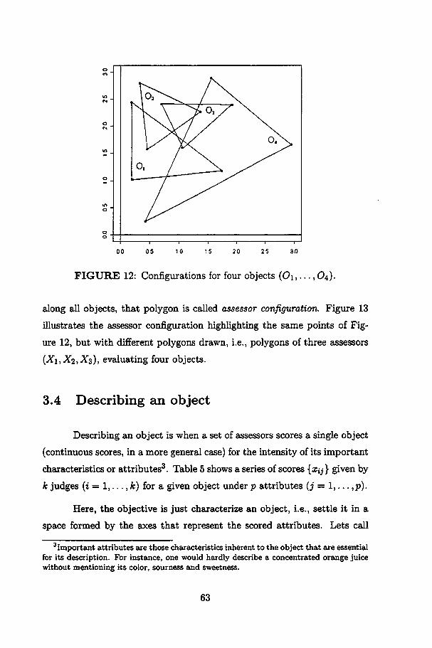
00 05 10 20 25 3.0
FIGURE 12: Configurations for four objects (Oi, ...,04).
along ali objects, that polygon is called assessor configuration. Figure 13
iUustrates the assessor configuration highUghting the same points of Fig
ure 12, but with different polygons drawn, i.e., polygons of three assessors
(X\,X2,Xz), evaluating four objects.
3.4 Describing an object
Describing an object is when a set of assessors scores a single object
(continuous scores, in a more general case) for the intensity of its important
characteristics or attributes3. Table 5 shows a series ofscores {x^} given by
k judges (i = 1,..., k) for a given object under p attributes (j = 1,... ,p).
Here, the objective is just characterize an object, i.e., settle it in a
space formed by the axes that represent the scored attributes. Lets call
3Important attributes are those characteristics inherent to the object that are essentialfor its description. For instance, one would hardly describe a concentrated orange juicewithout mentioning its color, sourness and sweetness.
63
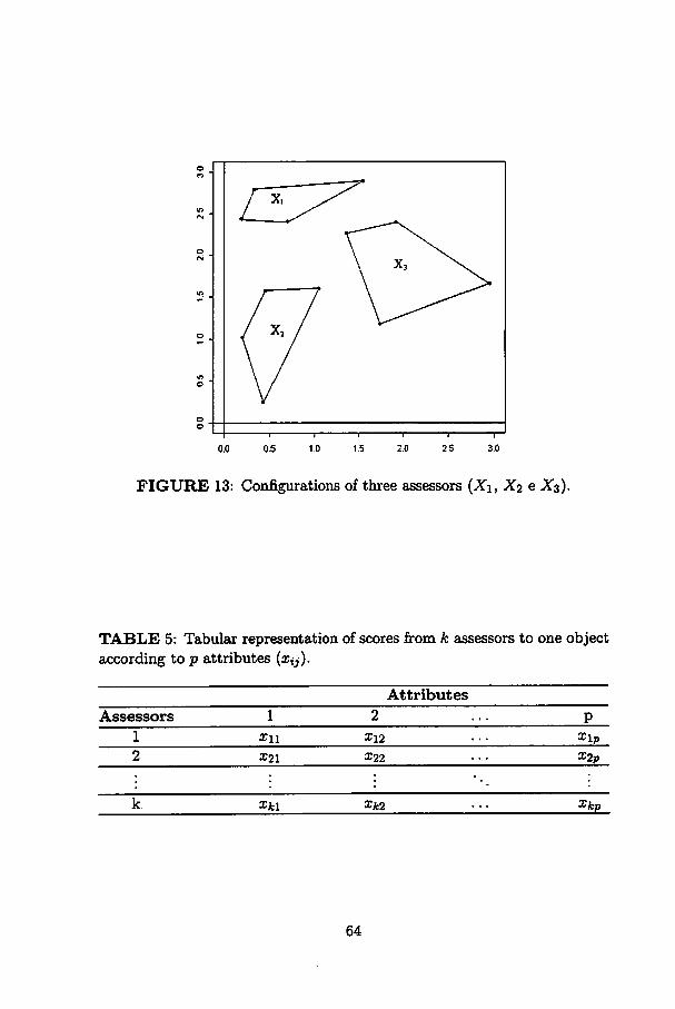
0.0 05 1.0 1.5
-T r-
25 30
FIGURE 13: Configurations of three assessors (X\, X2 e X$).
TABLE 5: Tabular representation of scores from k assessors to one objectaccording to p attributes (xíj).
Attributes
Assessors 1 2 P
1 Xu X12 X\p
2 £21 X22 X2p
'. '. '. ' • '•
k Xkl S*2 Xkp
64
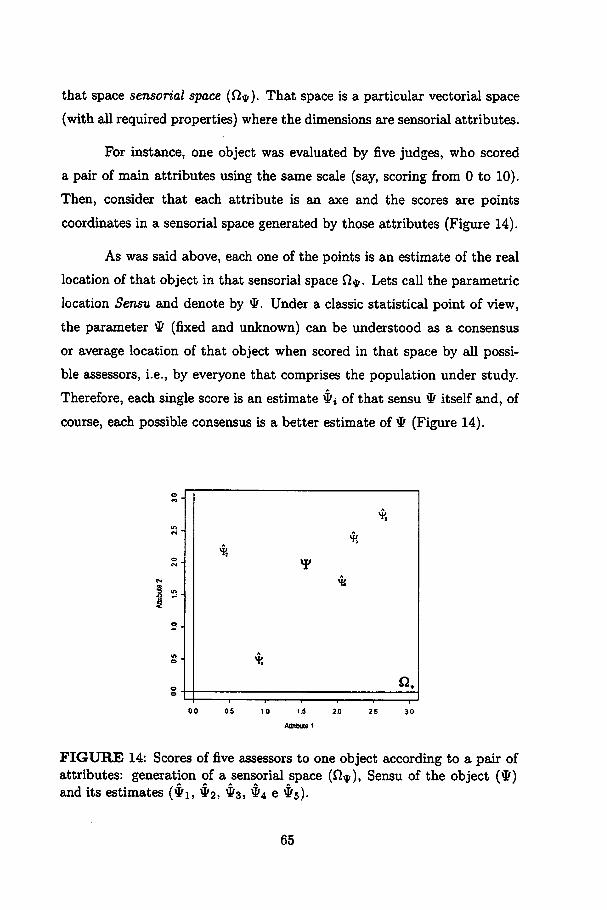
that space sensorial space (Qy). That space is a particular vectorial space
(with aU required properties) where the dimensions are sensorial attributes.
For instance, one object was evaluated by five judges, who scored
a pair of main attributes using the same scale (say, scoring from 0 to 10).
Then, consider that each attribute is an axe and the scores are points
coordinates in a sensorial space generated by those attributes (Figure 14).
As was said above, each one of the points is an estimate of the real
location of that object in that sensorial space Q^. Lets call the parametric
location Sensu and denote by $. Under a classic statistical point of view,
the parameter $ (fixed and unknown) can be understood as a consensus
or average location of that object when scored in that space by ali possi
ble assessors, i.e., by everyone that comprises the population under study.
Therefore, each single score is an estimate ^ of that sensu * itselfand, of
course, each possible consensus is a better estimate of $ (Figure 14).
I 3
"
%
%%
- ¥
-
$
- $,
Q,
10 1.5
Atmtxxoi
FIGURE 14: Scores of five assessors to one object according to a pair ofattributes: generation of a sensorial space (íl*), Sensu of the object (#)and its estimates (íj, $2) *3. *4 e $5).
65
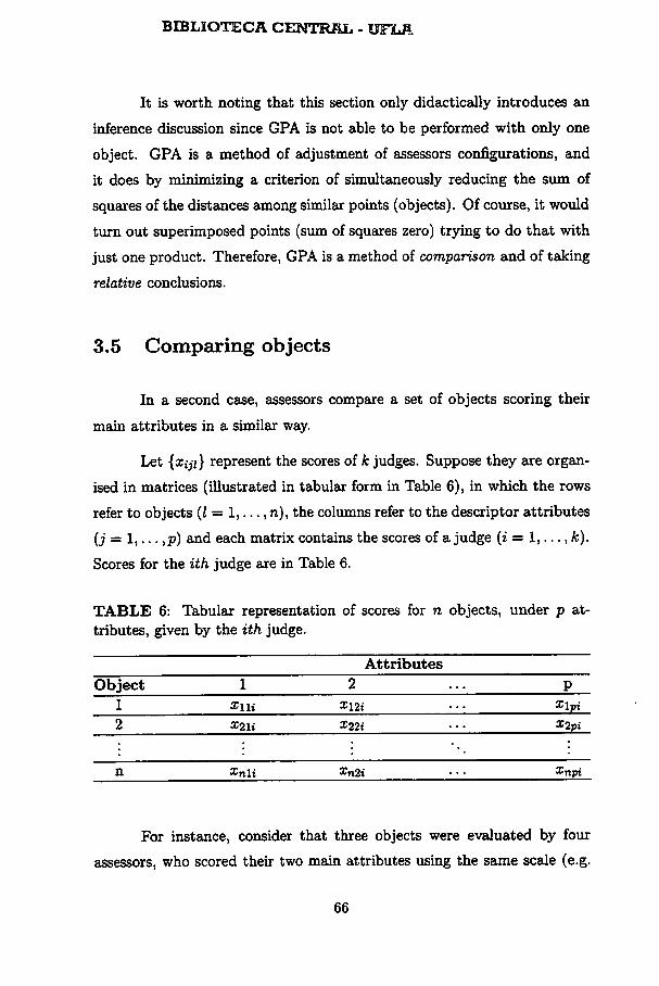
BIBLIOTECA CENTRAL - UVLR
It is worth noting that this section only didactically introduces an
inference discussion since GPA is not able to be performed with only one
object. GPA is a method of adjustment of assessors configurations, and
it does by minimizing a criterion of simultaneously reducing the sum of
squares of the distances among similar points (objects). Of course, it would
turn out superimposed points (sum of squares zero) trying to do that with
just one product. Therefore, GPA is a method of comparison and of taking
relative conclusions.
3.5 Comparing objects
In a second case, assessors compare a set of objects scoring their
main attributes in a similar way.
Let {xíji} represent the scores of k judges. Suppose they are organ-
ised in matrices (illustrated in tabular form in Table 6), in which the rows
refer to objects (l = 1,..., n), the columns refer to the descriptor attributes
(j = 1,... ,p) and each matrix contains the scores of a judge (i = 1,..., k).
Scores for the ith judge are in Table 6.
TABLE 6: Tabular representation of scores for n objects, under p attributes, given by the ith judge.
Attributes
Object 1 2 P
1 xm X\2i X\pi
2 X2\i X22i X2pi
'. ' • * • •
n Xnli Xn2i Xnpi
For instance, consider that three objects were evaluated by four
assessors, who scored their two main attributes using the same scale (e.g.
66
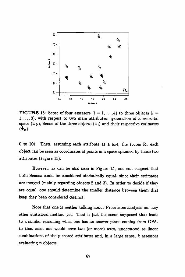
2 2'C
S
%
% yg
%
% %
^ *. ^
^ %
% %Q.
—i 1 1 1 1 1—
0.0 0.5 10 15 20 2.5 3.0
FIGURE 15: Score of four assessors (i = 1,... ,4) to three objects (l =1,...,3), with respect to two main attributes: generation of a sensorialspace (íí*), Sensu of the three objects (#/) and their respective estimates
0 to 10). Then, assuming each attribute as a axe, the scores for each
object can be seen as coordinates of points in a space spanned by those two
attributes (Figure 15).
However, as can be also seen in Figure 15, one can suspect that
both Sensus could be considered statistically equal, since their estimates
are merged (mainly regarding objects 2 and 3). In order to decide if they
are equal, one should determine the smaller distance between them that
keep they been considered distinct.
Note that one is neither talking about Procrustes analysis nor any
other statistical method yet. That is just the scene supposed that leads
to a similar reasoning when one has an answer plane coming from GPA.
In that case, one would have two (or more) axes, understood as linear
combinations of the p scored attributes and, in a large sense, k assessors
evaluating n objects.
67
3.6 GPA and Inference
Prior to GPA, let Xi (i = 1,..., k) denote a (nxp) matrix containing
information (for instance, scores) about n products in n dimensions, given
by the ith assessor. So, one could say that Xi represents the ith assessor,
since ali its entries come from him/her.
On the other hand, when one defines
k
t=i
Yi (k x p) refers to the information for the Ith product, each row coming
from one assessor; ei (i=l,.. • ,k) and ei (l = 1,... ,n) are vectors of zeros
with one in the ith and Ith position (i = 1,..., k and l = 1,..., n).
Now, reconsider the Procrustes problem (2.3),
k
/(si,...,s*,^,...,^Ti,..,,riO =£||si^i<i'
where Xi is a known nxp data matrix; $i is a scaling factor; Ui is a
translation vector; and Ti is a general transformation matrix (i < i' =
1,...,*).
Lets call X transformed, X\, the information matrix Xi after ali
transformation set in (2.3),
X\ = Sí(Xí - lu\)Ti.
In turn, one could think about the Y\ matrix for transformed con-
68
figurations.
t=l
k
=£wí(**-l^)Ti. (3.2)i=l
In practical situations, the probability distribution of the rows of
Yi is not known. Even if it was, it is not straightforward deriving the
distribution for the rows of Y{. Though Yf is function of Xi just like
Yi, the transformations of translation, scaHng, rotation, reflection etc, are
customized per row of Xi, i.e. per assessor. Then, it is not possible to
rewrite explicitly Y{ as function of Yj. Therefore, even if the distribution
of the Yi rows was known, the distribution of Y* rows was not. That is a
great motivation for using intensive computational techniques.
Automatically, it is impossible to derive algebraic expressions for the
distributions of the consensus (G), i.e. of the rows (estimates of products
locations), which is the estimator one is interested in to infer about,
k k
G={£,si(Xi-lvl)Ti =±'£xÍ.i=l i=l
In fact, one would want to derive simultaneously one probability
distribution for each G row, in order to make inference (estimation and
decision) for the n products at once. Since it is not possible, or at least
not straightforward, to do that algebraically, resampling techniques can be
used through intensive computational methods.
3.7 Monte Cario simulation
Monte Cario simulation is usually used as a first evaluation of new
strategies and decision rules before take the risk to try them in real situa-
69
tions (Miranda, 2004).
Monte Cario utilizes computational resources to generate samples
according to theoretical known distributions in order to evaluate the be-
haviour of statistical techniques for validate them, i.e., enable them to be
used in practical situations (Dachs, 1988).
3.8 Permutation tests
Permutation tests are computational efforts largely used to empir-
ically validate methods and/or test hypothesis. According to Gower &
Dijksterhuis (2004), the idea of permutation tests is to destroy the corre-
spondence between the rows of the data matrices. In the GPA framework
this means that the rows of the matrices Xi are permuted. The number
of variables p in a matrix Xi is of no importance for the permutation tests
since only the rows are permuted; it is immaterial whether the number pi of
variables in each Xi is constant. The set of ali possible permutations of N
rows of k matrices contains (n\)k permutations which will often be fax too
large a number to handle, so a much smaller random subset of permutations
is used. Each permuted data set has a particular RSS, say crs, associated
with it (s = 1, ..., 100, say). The value associated with the unpermuted
data set is called the empirical value, ao- A certain significance value, can
be attributed to the empirical value obtained. With RSS, the probability
P (as > ao) gives the significance.
The null hypothesis is that ao is not different from the other values
aa. Gower & Dijksterhuis (2004) say that when this is true it means that
GPA did not find any correspondence between the matrices Xi, but from
another point of view, it can be considered that permutating the rows within
matrices means to impose that ali products are the same, i.e. Ho: ao = as
means fio: *i = ^2 = ••• = *m where \&/ stands for the Ith product.
70
When p —value is small, say less than 5%, the empirical value ao
lies in the tail of the distribution of as values. In this case it may be judged
that there is likely to be a correspondence between the matrices detected by
GPA and/or also means to admite that, at least, two objects are different.
It is worth noting that the same investigation about the equality of
objects can be done, in a very similar way, through bootstrap procedures.
Virtual paneis can be easily resampled from the original data "mixing" the
rows for imposing equality of objects and producing a similar distribution
of RSS and computing P (as > ao). The same interpretations follow.
3.9 Bootstrapping
The technique of bootstrapping was first considered in a systematic
manner by Efron (1979), although the generality of the method means that
it was used in some particular circumstances before that time. The essence
of bootstrapping is the idea that in the absence of any other knowledge about
a population, the distribution of values found in a random sample of size
n (X\,...,Xk) from the population is the best guide to the distribution in
the population. Therefore, to approximate what would happen if the popu
lation was resampled it is sensible to resample the sample. In other words,
the infinite population that consists of the n observed values, each with
probability l/n, is used to model the unknown real population. The sam
pling is with replacement, which is the only difference in practice between
bootstrapping and randomization in many applications (Manly, 1998).
Let 9 be a parameter of interest and 9r its point estimate, called
here reference estimate. To apply the bootstrap technique one draw sev
era! (e.g. thousands) of bootstrap estimates of the particular parameter 6b,
b — l,...,B, with replacement. Such bootstrap estimates generate the so
called bootstrap distribution or empirical distribution of the estimator 9.
71
Such a distribution can be used to perform bootstrap hypothesis tests and
construct bootstrap confidence intervals for the parameter or functions of
the parameter of interest (Efron, 1993).
3.9.1 Confidence regions estimation
The simplest method for obtaining bootstrap confidence limits is
called the standard bootstrap method (Manly, 1998). The principie here is
that if an estimator 9 is normally distributed with mean 9 and standard
deviation a, then there is a probability of 1 - a that the statement
[9 - z°a <9<9+z°a) =1- a,
holds for any random value of 9, where z& is the value that is exceeded
with probability f for the standard normal distribution. This statement is
equivalent to
P(ê - z^a <9 <9 +z°a) =1- a,which therefore holds with the same probability, i.e., determining a 100(1 —
a)% confidence interval.
With the standard bootstrap confidence interval, a is estimated by
the standard deviation of estimates of a parameter 9 that are found by
bootstrap resampling of the values in the original sample of data,
a =
The interval is then
6=1
B-l
9±z° x (Bootstrap Standard Deviation)
72
The requirements for this method to work are that:
(a) 9 has an approximately normal distribution;
(b) 9 is unbiased so that its mean value for repeated samples from the
population of interest is 9;
(c) bootstrap resampling gives a good approximation to a (Efron, 1979).
Percentile method (Efron, 1979) determines a 100(1 —a)% confidence in
terval setting as upper and lower limits the bootstrap estimates that contain
between them 100(1 - a)% of the ordered bootstrap estimates.
If a increasingly monotonic function exists, such that the trans
formed estimates f(9) are normally distributed with mean f(9) and stan
dard deviation 1, then the mathematical form of the transformation does
not need to be known.
Therefore,
P(f(9) -z«< f(9) <f(9) +zf) =1- a
and then,
P(f(9) -z%< f(9) <f(9) +za) =l- a.
If the function /(•) is known, one just need to apply the inverse to obtain
the confidence interval for 9. However, that function is usually unknown.
Then, one way of deriving the confidence interval for f(9) is to resample
the original sampleand find the limits that exceed § (lower limit) and 1- §
(upper limit) of the transformed values.
However, due to the monotonic nature of the transformation func
tion, the order of the transformed bootstrap estimates /(0&) is the same as
non-transformed 9b- Therefore, a/2 and 1 - a/2 limits can be set on the
ordered bootstrap estimates and no transformation is necessary anymore.
73
According to Miranda (2004), there are so many other rules for con-
structing bootstrap confidence intervals, like HalTs (1992), which is based on
the same arguments of Efron (1979), but deals with residuais distribution.
3.9.2 Hypothesis testing
According to Manly (1998), bootstrap tests of significance have not
been as well studied as bootstrap confidence intervals, although they repre
sent an obvious application of the basic idea. Indeed, one way to carry out
a bootstrap test of the hypothesis that the parameter 9 takes the particular
value 9o involves simply calculating a bootstrap confidence interval for 9 and
seeing whether this includes 9q. This appears to indicate that the extension
of the theory of bootstrapping to tests of significance is trivial. However,
there is an important difference between the two applications that needs
to be recognized. This is that when carrying out a test of significance it is
important to obtain accurate estimates of criticai values of the test statistic
even if the null hypothesis is not true for the population from which the
sample being bootstrapped carne from. Basically it is a question of deciding
exactly how the null hypothesis being tested should influence the choice of
the statistic being bootstrapped.
Whatever test statistic 5 is used, a bootstrap test involves seeing
whether the value of S for the available data is sufficiently extreme, in
comparison with the bootstrap distribution of S, to warrant rejecting the
null hypothesis. Generally the test can operate in a similar way to a ran-
domization test. Thus suppose that large values of S provide evidence
against the null hypothesis. Then the observed data provide a value S\
of S, and bootstrap resampHng of the data produces another B —l values
S2,Sz,...,Sb- Ali B test statistics are from the same distribution if the
null hypothesis is true. Hence, S\ is significantly large at the 100a% levei
if it is one of the largest 100a% of the B test statistics. Or, to put it a
74
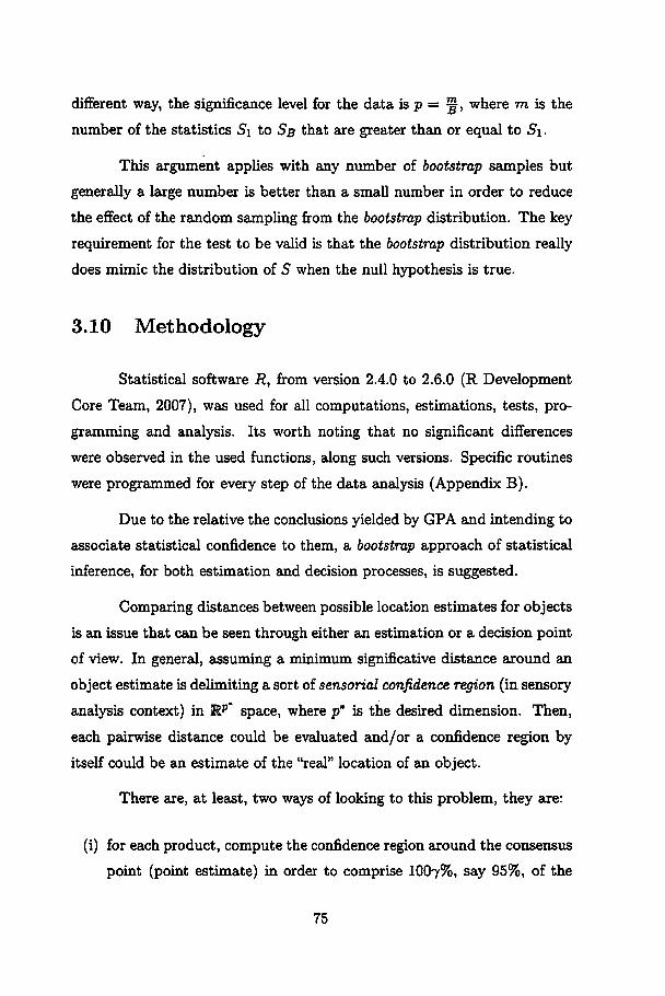
different way, the significance levei for the data is p = §, where m is the
number of the statistics Si to Sb that are greater than or equal to S\.
This argument applies with any number of bootstrap samples but
generally a large number is better than a small number in order to reduce
the effect of the random sampling from the bootstrap distribution. The key
requirement for the test to be valid is that the bootstrap distribution really
does mimic the distribution of S when the null hypothesis is true.
3.10 Methodology
Statistical software R, from version 2.4.0 to 2.6.0 (R Development
Core Team, 2007), was used for ali computations, estimations, tests, pro-
gramming and analysis. Its worth noting that no significant differences
were observed in the used functions, along such versions. Specific routines
were programmed for every step of the data analysis (Appendix B).
Due to the relative the conclusions yielded by GPA and intending to
associate statistical confidence to them, a bootstrap approach of statistical
inference, for both estimation and decision processes, is suggested.
Comparing distances between possible location estimates for objects
is an issue that can be seen through either an estimation or a decision point
of view. In general, assuming a minimum significative distance around an
object estimate is delimiting a sort of sensorial confidence region (in sensory
analysis context) in Rp" space, where p* is the desired dimension. Then,
each pairwise distance could be evaluated and/or a confidence region by
itself could be an estimate of the "real" location of an object.
There are, at least, two ways of looking to this problem, they are:
(i) for each product, compute the confidence region around the consensus
point (point estimate) in order to comprise 1007%, saY 95%, of the
75

possible point estimates generated by resampHng the actual scores
and then performing GPA (Figure 16a);
(ii) for each possible pair of point estimates (products), test the signif
icance of the sample (reference) euclidian distance, by comparing it
with quantiles of a distribution of euclidian distances under Hq (Fig
ure 16b).
For both situations, intensive computational techniques (as boot
strapping) are suitable due to the difficult to derive algebraically the distri
bution of such distances since the scores of each assessor suffer particular
transformations during the match process of GPA (Section 3.6).
However, the huge number of possible bootstrap tests (Cn,2) required
by the approach (ii) can turn it very hard to be performed; since it is usual
to evaluate 12, 16 or even 60 objects in an experiment (Dijksterhuis, 1995),
yielding 66, 120 and 1770 tests, respectively.
For that reason, it is preferred estimating the bootstrap confidence
regions for the sensus estimates and perform tests for the eucUdian distances
only between those products for which the equality is suspected, i.e. for
which the confidence regions touch each other.
That recommendation is made since the worst error in Sensory Anal
ysis is usually the Type H error, in the following pair of hypothesis
Ho : Both objects are equal
H\ : Both objects are different.
Under a rigorous point of view, i.e. at infinity precision, any pair of objects
is different. Therefore, committing Type I error, i.e. affirm that the objects
are different when they are not, is not a serious error. However, asserting
that two objects are the same, or at least undistinguishable according under
a specific vocabulary, requires one to be very sure about that.
76
. ^ \
1 -
/ V". . .♦.. A
\': *• •*• * •* i
f* -
i
i i i i
p pf r£**F*F FFF F
F* FF F
T-
Eixo principal1
(a)
«lJM
Eixoprincipal 1
(b)
FIGURE 16: (a) Sensorial confidence region for one object comprising1007% of the data generated by resampling one group average configuration('mean' scores through assessors). (b) Illustration of the bootstrap distancebetween supposed objects F and G.
77
It is useful and important to predict the (empirical, in this case) size
of the test (a) and its power (1 —0) in some basic situations. That can be
done using Monte Cario methods of simulation.
One can compute several simulated random samples of scores and
perform bootstrap inference (estimation and decision) of GPA accounting for
the percentage of times it agrees with the "truth". Let a be the probability
of incurring in Type I error. An estimator of a (à) can be the average
percentage of times that Type I error occurs, i.e. the null hypothesis (ali
objected are the same) is rejected when it is true. Consequently, that is
an estimator of the size of that test as well. Let 0 be the probability of
incurring in Type II error. An estimator of 0, say 0, can be the average
percentage of times that, when accepting fio that decision is found to be
false, i.e. Type II error occurs. Consequently, one an estimator of the power
of that test is 1 - 0.
3.10.1 Estimation
One can estimate the confidence region for each point (object) via
bootstrap. The idea is to resample, with replacement, the information (e.g.
scores) matrices, each one representing a subject.
A discussion on the ideal resample unit is pertinent. Here, one is
considering the whole data matrix Xi as the resample unit. That agrees
with Husson et ai. (2005) when estimating confidence ellipses for sensory
profiles obtained by principal component analysis by bootstrapping. In fact,
that resample unit seems to provide suitable estimates. However, more
work is required in this issue. For instance, when one experiment has a
small number of assessors, resampling the whole matrix Xi can lead to
several identical estimates since many identical virtual paneis are going
to be formed. It can compromise the reliability of bootstrap results. Of
course, the main cause for a poor reliability in this situation is the small
78
size of original sample. However, in those cases a more efficient resample
unit must be searched. When the assessors scores have high correlation
among each other, e.g. they were equally well trained, resampling rows or
matrices produces nearly the same result. That happens because the new
virtual assessor formed is very similar to a real one. If one resample rows
in a low between-assessors correlation context, the virtual assessor formed
would be fax different from the rest of the panei, leading to inadequate
estimates. In situations where the between-assessors correlation is high
enough, the practice of resampling rows would round the low degrees of
freedom problem.
ResampHng with replacement one builds up a bootstrap sample (vir
tual panei) with the same size of the original one. That process is repeated
several times and, for each bootstrap sample set up, one Generalised Pro
crustes Analysis is performed and the group average configuration com-
puted. After produced several virtual paneis, and therefore group average
configurations, an ultimate GPA for adjusting ali group (bootstrap -f sam
ple) averages and referring everyone to the same coordinate system. After
that, one can see a cloud of points "around" the sample estimates.
For those points referred to the same axes, one can determine a
1007% confidence bootstrap confidence region, i.e. containing 1007% of the
estimates for each product. When those points follow a symmetric bivariate
distribution (for instance, Gaussian distribution), it is straightforward es
timating that region through an bootstrap confidence ellipse (Figure 17a)4.
Note that, if a vector Z contains p coordinates of a point that fol-
lows a multivariate Normal distribution N(/jl, E), with mean vector fj, and
4R packagecalled ellipse bringsa set offunctions forestimating ellipses. One of them,with the same name, fits perfectly the present situation.
79
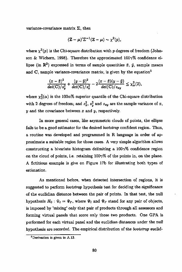
variance-covariance matrix S, then
(Z-m/S-^Z-m)-*^),
where x2(p)1S the Chi-square distribution withp degrees of freedom (John
son & Wichern, 1998). Therefore the approximated 1007% confidence el
lipse (in R2) expressed in terms of sample quantities x, y, sample means
and C, sample variance-covariance matrix, is given by the equation5
(x-x)2 , (y-yf n(x-x)(y-y) ^_2/m+ j^/^\/-2 _ 2~7ZI77=^T. ^ Xq(2),det(C)/s2 det(C)/s2 det(C)/ssy
where x2(a) 1S *^e lOO^^o superior quantile of the Chi-square distribution
with 2 degrees offreedom; and s2, s2 and sxy are the sample variance ofx,y and the covariance between x and y, respectively.
In more general cases, like asymmetric clouds of points, the ellipse
fails to be a good estimator for the desired bootstrap confident region. Thus,
a routine was developed and programmed in R language in order of ap-
proximate a suitable region for those cases. A very simple algorithm allows
constructing a bivariate histogram delimiting a 1007% confidence region
on the cloud of points, i.e. retaining 1007% of the points in, on the plane.
A fictitious example is give on Figure 17b for illustrating both types of
estimation.
As mentioned before, when detected intersection of regions, it is
suggested to perform bootstrap hypothesis test for deciding the significance
of the euclidian distance between the pair of points. In that test, the null
hypothesis Ho : Wi —*//, where */ and ty/ stand for any pair of objects,
is imposed by 'mixing' only that pair of products through ali assessors and
forming virtual paneis that score only those two products. One GPA is
performed for each virtual panei and the euclidian distances under the null
hypothesis are recorded. The empirical distribution of the bootstrap euclid-
5Derivation is given in A.13.
80
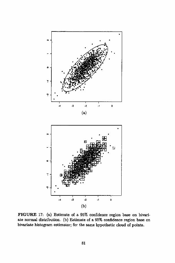
(b)
FIGURE 17: (a) Estimate of a 95% confidence region base on bivariate normal distribution. (b) Estimate of a 95% confidence region base onbivariate histogram estimator; for the same hypothetic cloud of points.
81

ian distances is displayed highHghting the position of the sample eucHdian
distance. After that, the sample eucHdian distance is considered significant
if 1007% of the bootstrap eucHdian distances are less than it. The decision
process is detailed in the next section.
It is worth stressing that GPA conclusions under the proposed boot
strap inference method do not loose their relative feature. During the whole
method, what is estimated or tested is the relative location of objects and
the distance between objects in a generally scaled Rp coordinate system.
In other words, the scale is immaterial for conclusions.
3.10.2 Decision
Let 6 be the eucHdian distance between a pair of products. The sam
ple provides an reference estimate (6r) of the parametric eucHdian distance,
according to a set of assessors.
Based on that, some hypothesis can rise. Consider the following
plausible pair of hypothesis fio and H\:
*!,-°. (3.3)Hi : 6 > 0
Hypothesis fio states that the pair of evaluated products are equal.
Of course, 6 will hardly be exactly zero. Statement (3.3) turns clear that
6 —0. In other words, the reference euclidian distance is statistically equal
to those found when the products are imposed to be the same.
That can be done by "mixing" the scores of a specific pair of objects
ali together and drawing them with replacement for composing virtual pan
eis, new scores matrices. By scores to be mixed is meant the entire rows of
the actual matrices of scores, i.e. the vector of coordinates for a product,
along ali assessors.
82
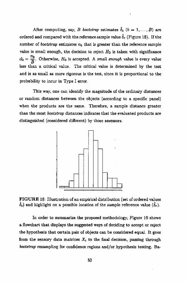
After computing, say, B bootstrap estimates <5& (6 = 1,..., B) are
ordered and compared with the reference sample value ÔT (Figure 18). If the
number of bootstrap estimates nj, that is greater than the reference sample
value is small enough, the decision to reject fio is taken with significance
âb = —. Otherwise, fio is accepted. A small enough value is every valueB
less than a criticai value. The criticai value is determined by the test
and is as small as more rigorous is the test, since it is proportional to the
probability to incur in Type I error.
This way, one can identify the magnitude of the ordinary distances
or random distances between the objects (according to a specific panei)
when the products are the same. Therefore, a sample distance greater
than the most bootstrap distances indicates that the evaluated products are
distinguished (considered different) by those assessors.
d
FIGURE 18: Illustration of an empirical distribution (set of ordered valuesôb) and highlight on a possible location of the sample reference value (o>).
In order to summarize the proposed methodology, Figure 19 shows
a flowchart that displays the suggested ways of deciding to accept or reject
the hypothesis that certain pair of objects can be considered equal. It goes
from the sensory data matrices Xi to the final decision, passing through
bootstrap resampling for confidence regions and/or hypothesis testing. Ba-
83
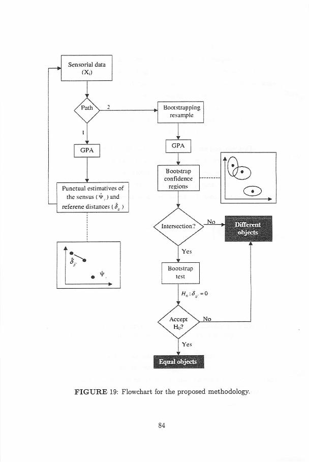
Sensorial data
CXj)
Path
GPA
Punctual estimatives of
the sensus (*P,) and
referene distances ( 8,. )
Bootstrappingresample
GPA
Bootstrapconfidence
regions
Equal objects
FIGURE 19: Flowchart for the proposed methodology.
84
sically, the flowchart is formed by two (didactically distinct) parts: (1) point
estimation of the location of the evaluated objects in a sensory space; and
(2) estimation of sensory confidence regions and bootstrap tests. When one
decides going on path 1, conventional GPA is performed and, obligatorily
one has to return to initial data for path's 2 procedure. On path 2, bootstrap
resampling provides the generation of several virtual paneis which deter
mine the bootstrap confidence regions estimates. Then, visual inspection
for intersection of confidence regions can be done. In visual inspections for
each pair of objects is made a decision whether their are different or further
investigation can be done. When the later option is chosen, a bootstrap hy
pothesis test is performed for each pair of objects for which the equality is
suspected. It is worth noting that there is no impediment to test the equal
ity hypothesis even when there is no intersection of the confidence regions,
however that action does not counts for optimizing the process.
3.10.3 Algorithm
This section aims to summarize the proposed method in form of
algorithm. Steps are as follow:
(1) Group the information about n objects. under p dimensions, given byk assessors in k matrices nxp;
(2) Perform GPA on sample data and compute the group average configuration Gs;
(3) Resample the matrices of original data forming a virtual panei. PerformGPA in that panei and compute the group average configuration Gbi;
(4) Repeat (3) a high enough number of times B yielding Gbi, Gb2, ---, GbB\
(5) Perform an ultimate GPA on {Gs,Gb\, • •• ,GbB} and reduce the di-mensionaHty to a low number (e.g. two) of dimensions, in order toconcentrate the variation for plotting;
(6) Construct 1007% confidence regions (not necessarily eUipses) for theith object (i = 1,..., n);
85
(7) If no elHpses intercept each other the process stops and (besides usualconclusions) the objects are said to be distinguishable. Otherwise, goto (8);
(8) Test each pair of intercepted eUipses by imposing Ho of equality. It isdone "mixing" only two such rows among assessors and producing virtual paneis. Then, for each virtual panei produced, a GPA is performedand the negHgible distance between such pair of objects is computed.After a sufficient number of distance computed, the sample distance iscompared with the empirical distribution of distances under Ho. Percentage of values greater than the sample distance is understood as anexact p-value. Normal decisions are made confirming or refuting thesuspect of equality.
3.10.4 Practical experiments
Two practical data example were used to illustrate both confidence
region estimation and some hypothesis tests.
a) The first one was kindly available by Fernando A. R. Magalhães, from
EPAMIG/Instituto de Laticínios Cândido Tostes. It is regarded to sen
sory evaluation of gorgonzola cheese, from two distinct technologies.
Nine assessors scores eight different cheeses (4 ripening ages from each
technology) in a Quantitative Descriptive Analysis (QDA) context, ac
cording to ten attributes: appearance (Ap), amount of mold (AM),
texture (Tx), characteristic odor (CO), aroma (Ar), characteristic fla-
vor (CF), salty taste (ST), acid taste (AT), bitter taste (BT), residual
flavor (RF). Cheeses from 1 to 4 come from technology 1; and from 5
to 8 come from technology 2. Ripening ages are, respectively 30, 45, 60
and 70 days. Magalhães (2002) explore these data via univariate analy
sis of variance (ANOVA) and Ferreira (2004) analysed the same data set
through multivariate analysis of variance (MANOVA) and Generalised
86
Procrustes Analysis (GPA). However, conclusions can still be enhanced
with inference techniques.
b) The second example was kindly available by Wageningen Centre for
Food Sciences (WCFS) through Garmt Dijksterhuis, Pieter Vereijken
and Eric Dransfield. It is a two experiment data set were 90 naíve asses
sors were asked to evaluate 19 (9+10) commercial semi-solid food prod
ucts purchased in The Netherlands, basically custards, yoghurts, may-
onnaises (experiment 1) and fresh creams, soft cheeses and creams (ex
periment 2). They were evaluated according to a nine attribute vocab-
ulary: dairy taste (DT), thickness mouth-feel (TMF), airy mouth-feel
(AMF), melting mouth-feel (MMF), heterogeneity mouth-feel (HMF),
creamy soft mouth-feel (CMF), fatty mouth-feel (FMF), sticky mouth-
feel (SMF) and astringent mouth-feel (AsMF).
3.10.5 Simulation studies
Inspired by practical data sets two simulation studies were held to
vaHdate the described method and estimate the power and type I error
rates of the estimation and decision procedures.
a) Based on the Gorgonzola data set, virtual paneis were simulated from
multivariate Gaussian distributions. Their parameters (mean vectors
and variance-covariance matrices) were the sample mean vectors and
sample variance-covariance matrices from the practical data set. Data
set had 720 records from an experiment of 8 products x 9 assessors x
10 attributes. The reason of simulating from Normal distributions was
that it is the more used and well known distribution and it has the good
properties.
Xi ~ N(jh = xí, Si = Si), i = 1,..., 8.
87
Five hundred virtual paneis were simulated under complete alternative
hypothesis H\ : *i ^ $2 7^ • • # %N and the bootstrap inference
method was performed in order to evaluate the power rate. Percentage
of wrong decisions was accounted in each step (estimation and decision)
and in the whole process.
b) In order to better explore the behaviour of the described method, an
other simulation study was held. Six products were carefully chosen
from the Dutch dairy sensory experiment: products 1, 2, 4 and 6 from
the first experiment and products 5 and 7, from the second one. From
now on, they are referred as products 1 to 6, respectively.
In this simulation study, the partial Hq : #1 # $2 # *3 = ^4 # *5 =
$6 was imposed. For products 1 e 2, were considered the sample mean
vectors and the sample variance-covariance matrices. For pairs (3,4)
and (5,6), were considered the average of the sample mean vectors and
the average of the sample variance-covariance matrices, for each pair.
Therefore, three distinct groups wereformed: (i) $1 ^ #2; (ü) *3 = #45
and (iii) #5 = *6 (Figure 20).
W2 ~ N(fi2 = X2,S2 = S2)
W3, W4 ~ iV(/i3(4 = X3,4, Z3.4 = 5s,4)
W5, Wq ~ N(/i5)6 = X5>6,£5,6 = S5,e)
where Wi (l = 1,2,..., 6) are random vectors of length p —9.
For sample sizes of k = 5,10,15,20,50,90 assessors, five hundred repli-
cations were drawn and the described method was performed in order
to evaluate power and type I error rates.
Eight rates were measured at each replication for evaluating the be
haviour of the described method:
88
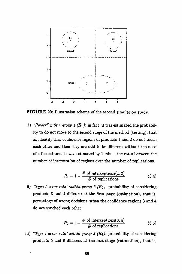
3.4
Group 2
5.6
Group 3
Group 1 1 2
FIGURE 20: Illustration scheme of the second simulation study.
i) "Power" withingroup 1 (Ri): in fact, it was estimated the probabil
ity to do not move to the second stage of the method (testing), that
is, identify that confidence regions of products 1 and 2 do not touch
each other and then they are said to be different without the need
of a formal test. It was estimated by 1 minus the ratio between the
number of interception of regions over the number of replications.
#1 = 1-
#2 = 1-
# of interceptions(l, 2)# of replications
ii) "Type I error rate" within group 2 (R2): probability of considering
products 3 and 4 different at the first stage (estimation), that is,
percentage of wrong decisions, when the confidence regions 3 and 4
do not touched each other.
# of interceptions(3,4)# of replications
iii) "Type I error rate" within group 3 (R$): probabiHty of considering
products 5 and 6 different at the first stage (estimation), that is,
89
(3.4)
(3.5)
percentage of wrong decisions, when the confidence regions 5 and 6
do not touched each other.
r = i _ # of interceptions(5,6)# of repHcations
iv) "Power" between groups (Ra): probability of considering the three
groups to be different at the first stage (estimation), that is, percent
age of correct decisions, when the confidence regions of the groups
do not touched each other.
# of interceptions between groups . .R4 = 1 — — ; (3.7)
# of replications
v) Type I errorrate within group 2 (R5): since one moved to the second
stage of the method (testing), percentage of times it rejects the null
hypothesis Ho : X$ = X4 (a = 5%).
R _ 1_ # of rejections of H0 :X3 = X4# of tests performed
vi) Type I error rate within group 3 (Re): since one moved to the second
stage of the method (testing), percentage of times it rejects the nuU
hypothesis Ho : X$ = Xe (a = 5%).
_ # of rejections of HQ :X5 = X6 , g.# of tests performed
vii) Whole type I error rate within group 2 (R7): summation of type
one error rates of the first (estimation) and second (testing) stages
of the inference method, for group 2.
R7 = R2 + R5 (3.10)
viii) Whole type I error rate within group 3 (Rs)- summation of type
one error rates of the first (estimation) and second (testing) stages
90
of the inference method, for group 3.
Rs = Rz + Re (3.11)
3.11 Results
According to the enumeration of the examples described in the
Methodology, the results and discussion follow. First, two practical experi-
ments are discussed: the Gorgonzola experiment with well trained assessors
(a) and the two Dutch commercial semi-solid foods experiments with 90 as
sessors (b).
3.11.1 Practical experiments
(a) Gorgonzola experiment (Ferreira et ai., 2007)
Figure 21, adapted from Ferreira (2004), shows the two principal
axes after Generalised Procrustes Analysis for eight gorgonzola cheeses (1
to 8), evaluated by nine assessor (A to /). Ferreira (2004) argues that,
sometimes, the location estimates for some products are so close that one
could think they are undistinguishable by the group consensus. Though
there are no so close estimates in this case one could wonder whether some
distances are significant (for instance, products 1 and 6 or 3 and 7). To
solve that problem one can, for instance, determine the confidence region
for each cheese based on their consensus estimates. Thus, 95% confidence
regions were built based on bivariate normal distributions. B = 100 virtual
paneis were formed drawing B bootstrap samples, with replacement, from
the original data set, performing B GPA's and computing their group av
erage configurations (Figure 22). Figure 22a shows 100 bootstrap estimates
(black numbers) and the sample reference estimate (white number), while
Figure 22b displays the same scene highHghting the bootstrap confidence re-
91

gions and the sample referenceestimates. Both biplots bring the attributes
(described in Section 3.10.4) positioning.
#CN _(N
C\J
to
'55
2 5$fc
CO ~ 7<77gEEr(0a
Dc
CL 4G %
1 1 I I
Principal axis 1 (64%)
FIGURE 21: Transformed scores for eight products (1 to 8), by nineassessor (A to I), on the response-plane of GPA.
As was said, looking to Figure 21, one could suspect that this panei
would confound products 1 and 6 or 3 and 7. That is not the same impres-
sion one has looking to Figure 22. Since there is no intersection between
eUipses, according to the proposed methodology (Figure 19), one could
conclude ali cheeses are distinguishable, with at least, 95% of confidence.
Although conclusions for this case seem to be clear, suppose one in-
sists in performing a test for the equality between the pairs of cheeses (1,6)
and (3,7). Figure 23 shows empirical distributions of eucHdian distances
between such pairs of cheeses, under the null hypothesis. They were com
puted from 500 ordered bootstrap observations of null euclidian distances.
The eucHdian distance between the pair (1,6), for them to be considered
undistinguishable, seems to be something around 0.09. Since the sample
eucHdian distance is more than 0.19 and according to the empirical distri
bution (a) of Figure 23, it is highlyadvisable do not to accept Hq : ôi$ = 0
92
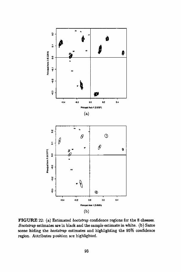
*» T.
AT
*
At
Ali
\i 1
-0.2 0.0 02
PrineptlAxis 1(0.6387)
(a)
_
*» T.A
JftT
COc*
8 %
-
A>
AM
1 r- 1
®-i—'
-0.2 0.0 02
PrintiptlA»* 1(0.6363)
(b)
FIGURE 22: (a) Estimated bootstrap confidence regions for the 8 cheeses.Bootstrapestimates are in black and the sample estimate in white. (b) Samescene hiding the bootstrap estimates and highHghting the 95% confidenceregion. Attributes position are highlighted.
93
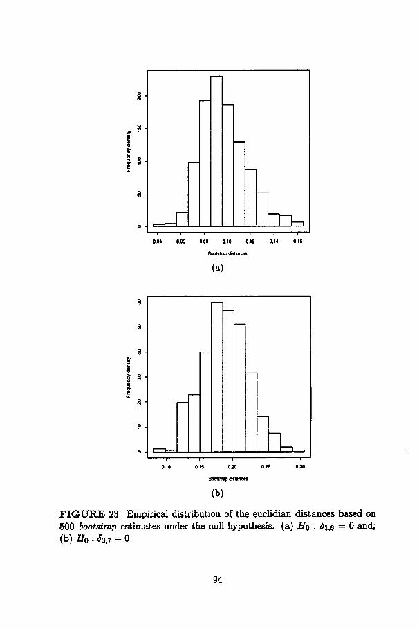
8-
Bootstrap distances
(a)
fr 8 -
0.25
Bootstrap distances
(b)
FIGURE 23: Empirical distribution of the eucHdian distances based on500 bootstrap estimates under the nuU hypothesis. (a) Ho : <5i,6 = 0 and;(b) Ho : (53,7 = 0
94
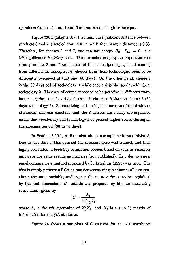
(p-value= 0), i.e. cheeses 1 and 6 are not close enough to be equal.
Figure 23b highHghts that the minimum significant distance between
products 3 and 7 is settled around 0.17, while their sample distance is 0.33.
Therefore, for cheeses 3 and 7, one can not accept Ho : £3,7 = 0, in a
5% significance bootstrap test. Those conclusions play an important role
since products 3 and 7 are cheeses of the same ripening age, but coming
from different technologies, i.e. cheeses from those technologies seem to be
differently perceived at that age (60 days). On the other hand, cheese 1
is the 30 days old of technology 1 while cheese 6 is the 45 day-old, from
technology 2. They are of course supposed to be perceive in different ways,
but it surprises the fact that cheese 1 is closer to 6 than to cheese 5 (30
days, technology 2). Summarizing and noting the location of the desirable
attributes, one can conclude that the 8 chesses are clearly distinguished
under that vocabulary and technology 1 do present higher scores during ali
the ripening period (30 to 75 days).
In Section 3.10.1, a discussion about resample unit was initiated.
Due to fact that in this data set the assessors were well trained, and then
highly correlated, a bootstrap estimation process based on rows as resample
unit gave the same results as matrices (not published). In order to assess
panei consonance a method proposed by Dijksterhuis (1995) was used. The
idea is simply perform a PCA on matrices containing in columns aU assessor,
about the same variable, and expect the most variance to be explained
by the first dimension. C statistic was proposed by him for measuring
consonance, given by
C AiTk A-'
where A» is the ith eigenvalue of XjXj, and Xj is a (nx k) matrix of
information for the jth attribute.
Figure 24 shows a bar plots of C statistic for ali 1-10 attributes
95
used in Gorgonzola evaluation. However, note that Figure 24a is a kind of
misleading. It is important tó say that the numbers 1 to 10 for attributes are
related to the order presented above, i.e. 1- appearance (Ap), 2— amount
of mold (AM), ..., 10- residual flavor (RF). Its smallest bar (attribute 9)
seems to indicate a variable poorly interpreted by the assessors, but its first
eigenvalue is 70 times greater than summation of the other ones! There is
a scale "problem" here, since the attribute 10 has a first eigenvalue 1500
times the sum of the other ones. In this practical example, ali attributes
are incredibly well understood and weU scored by the assessors. It seems to
be a weak point for Dijksterhuis' C statistic. When a attribute gets close
to the ideal situation, be explained in 1 dimension, Yii=2 ^* *s tmv> *ben C
tends to infinity. In order to turn them less misleading, Figure 24b shows
the same C statistics in a logarithm scale.
Another tools suggested by Dijksterhuis (1995) are a common scree
plot for ali attributes and plots of assessors space in order to search for bad
trained. As this situation shows to be close to ideal and ali attributes were
weU scored, scree plots are expected to be similar to each other and well
designed, as can be seen on Figure 25. For ali of them, the first dimension
explains very far the most variance and their explanation is very similar.
In Figure 25 it is really hard to check that attribute 10 behaves
better and attribute 9 is the worst. In order to explore in more details
the assessors behaviour per attribute is shown on Figure 26a and Figure
26b the positions of ali assessors in attributes 10 and 9 (better and worst,
respectively). Even in the worst consonance, the panei scored quite well,
i.e. Figure 26b shows assessors very close to the first dimension, indicating
a extraordinary overall panei consonance.
Another as interesting as expected feature is the variance accounted
for on the axes. As can be seen almost ali the variations is explained in the
first component, what confirms good training.
96
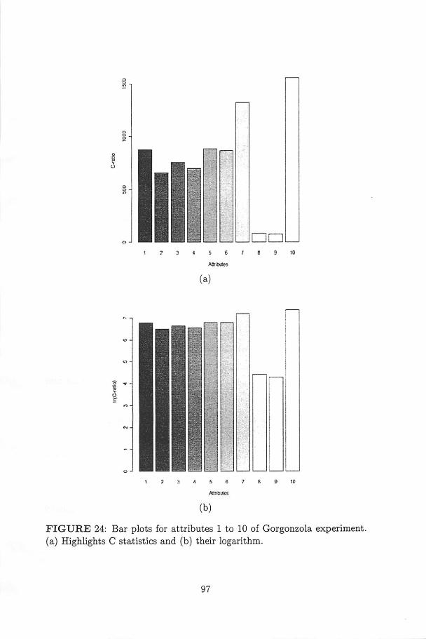
- ••
• •
17 3 4 5 6 /
AünWes
••
r—j |• - j
..-• .
•'-". I
. -tT"
1
l;- .1
I• • .j
]
| ;,: :";
6 6 7 8 9 10
AtWDUies
(b)
FIGURE 24: Bar plots for attributes 1 to 10 of Gorgonzola experiment.(a) Highlights C statistics and (b) their logarithm.
97
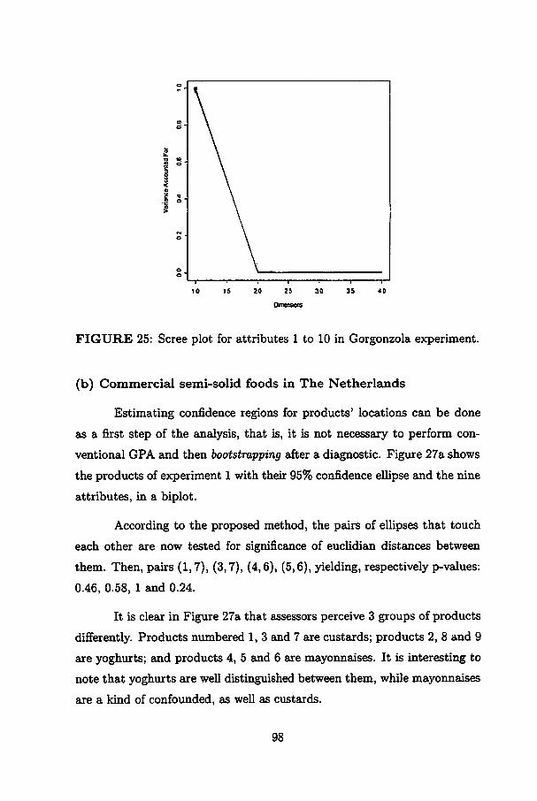
foncnsons
FIGURE 25: Scree plot for attributes 1 to 10 in Gorgonzola experiment.
(b) Commercial semi-solid foods in The Netherlands
Estimating confidence regions for products' locations can be done
as a first step of the analysis, that is, it is not necessary to perform con-
ventional GPA and then bootstrapping after a diagnostic. Figure 27a shows
the products of experiment 1 with their 95% confidence elHpse and the nine
attributes, in a biplot.
According to the proposed method, the pairs of elHpses that touch
each other are now tested for significance of eucHdian distances between
them. Then, pairs (1,7), (3,7), (4,6), (5,6), yielding, respectively p-values:
0.46, 0.58, 1 and 0.24.
It is clear in Figure 27a that assessors perceive 3 groups of products
differently. Products numbered 1, 3 and 7 are custards; products 2, 8 and 9
are yoghurts; and products 4, 5 and 6 are mayonnaises. It is interesting to
note that yoghurts are well distinguished between them, while mayonnaises
are a kind of confounded, as weU as custards.
98

•aO.
£
45 0.0 G 5
PnncipalAas 1(0.9994)
(a)
p .
|IO
Ii
jíj
o9
o 525
9*
p _
1—i i 1í í 1—'•06 00 05
PnnopsIAas 1{0 9004)
(b)
FIGURE 26: Assessors space for attributes 10 - residual flavor (a) and 9- bitter taste (b).
99

In turn, Figure 27b shows fresh creams, soft cheeses and creams.
Clusters here are not so well define as in Figure 27a, but the adicional
interpretation is quite interesting. Products 1 and 2 are fresh creams. Note
that they would not be well distinguished by a possible population those
assessors come from. Additionally, products 10, a soft cheese, is confounded
with them. Products 7, 8 and 9 are creams. Note that 7 and 9 are much
more similar than 8. A very far-from-everyone is product number 5, a
MozzareUa, that share few attributes with the other products. Finally, 3,
4 and 6 are cheeses probably with intermediate characteristics.
Again, products suspect of equality were tested by the bootstrap
hypothesis test algorithm. Proposed method was efficient for identifying
pairs (1,2), (2,10) and (1,10), as similar and testing them, yielding p-
values 1 (100%) for ali them. That confirms that these three products are
perceived the same way according to a specific vocabulary.
Investigating panei consonance, one can see a scene less "ideal" than
the Gorgonzola experiment. That is, assessors are less trained and therefore
agree less, in this case. It can be seen clearly on Figures 28 and 29.
In experiment 1, attribute 3 is the more unidimensional one. On the
other hand, attribute 6 presents itself a little bidimensional (Figure 28a),
even though its C is almost 5, that is, its first dimension explains almost
five times the sum of the other dimensions. Figure 28b shows the variance
explained by the first four dimensions for the nine attributes. Attribute
3 shows a high first dimension and a very low second one, what turns it
the better understood one. However, attribute 6, besides presenting the
lowest first dimension, its shows the higher second dimension, then it can
be considered to have the poorest understanding.
Figure 30a and 30b show the assessors' space for attributes 3 and 6,
respectively. Most unidimensional attribute 3 shows most of the assessors
scoring quite weU. However it can be identified assessors 74 and 82 scoring
100
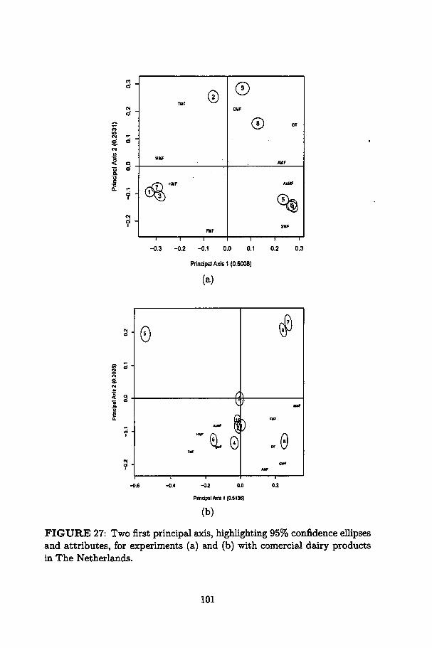
TBF ©©
CUF
© OT
UUfAMF
-«$"AtMF
I 1" •
FUF
• r 1
SMF
1 1
-0.3 -0.2 -0.1 0.0 0.1 0.2 0.3
0
Principal Axis 1 (0.5008)
(a)
í)
Q. 0
1
-02 0.0
Prinepal Axis 1(0.5136)
.0
-r-
02
(b)
FIGURE 27: Two first principal axis, highlighting 95% confidence ellipsesand attributes, for experiments (a) and (b) with comercial dairy productsin The Netherlands.
101
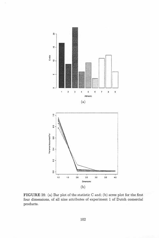
iO 2 5 3.0
Dimensions
(b)
FIGURE 28: (a) Bar plot of the statistic C and; (b) scree plot for the firstfour dimensions, of ali nine attributes of experiment 1 of Dutch comercialproducts.
102
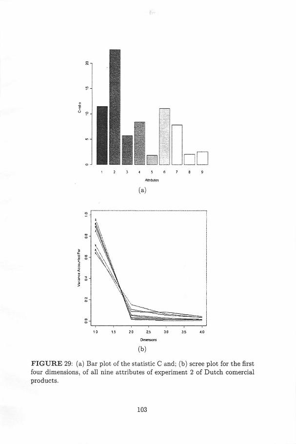
FIGURE 29: (a) Bar plot of the statistic C and; (b) scree plot for the firstfour dimensions, of ali nine attributes of experiment 2 of Dutch comercialproducts.
103
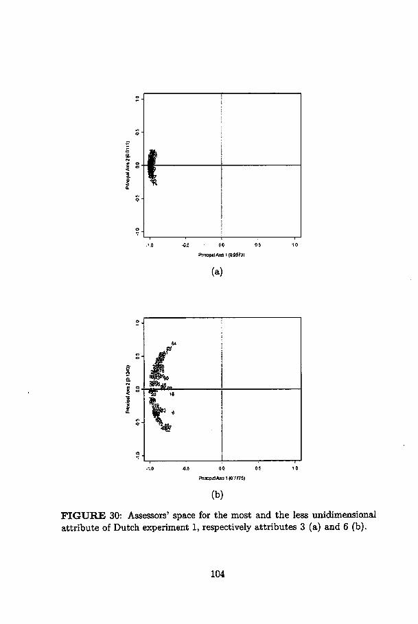
.
1s"^
00 05
PnncipalAns 1(05573)
(a)
•C.5 00 06
PnnapílAnS 1 (07775)
(b)
FIGURE 30: Assessors' space for the most and the less unidimensionalattribute of Dutch experiment 1, respectively attributes 3 (a) and 6 (b).
104

worst, that is, more bidimensional.
On the other hand, on Figure 30b can be seen that several assessors
are scoring attribute 6 in two dimensions. Assessors 64 and 82 (again) are
highlighted as the most discrepant ones.
In experiment 2, attribute 2 is by far the better understood, the
better expressed in one dimension. Its C is greater than 20, i.e. its first
dimension accounts more than 20 times the other ones (Figure 29a). The
same behaviour of attribute 2 is reproduced by Figure 29b, where it can be
seenit has the highest first dimension and the lowest second dimension. On
the other hand, although Figure 29a shows attribute 5 to have the lowest
first dimension, Figure 29b reveals attribute 9 to leave the great amount of
variation to be explained by the second dimension. Therefore, attribute 9
can be considered the more two dimensional attribute.
For the most unidimensional attribute (2), Figure 31a shows asses
sors 46 and 69 as the most bidimensional ones when scoring that attribute.
In turn, when scoring attribute 9, the most bidimensional one (Figure 31b),
several assessors seem to understand it wrongly, highlighting assessors 26,
61 and 78.
It is interesting comparing Figure 26b and Figure 31b. Note how
assessors are better trained in Gorgonzola's experiment. By the way, in
experiment with comercial Dutch products, the assessors are not specifically
trained. Even if they were, training 90 assessors would be a very harder
task than training nine.
3.11.2 Simulation studies
a) Along500drawings from multivariate Normal distributions, with
parameter coming from the Gorgonzola data set, the behaviour of the de-
scribed method was stable and well defined. Since the scores have come
105
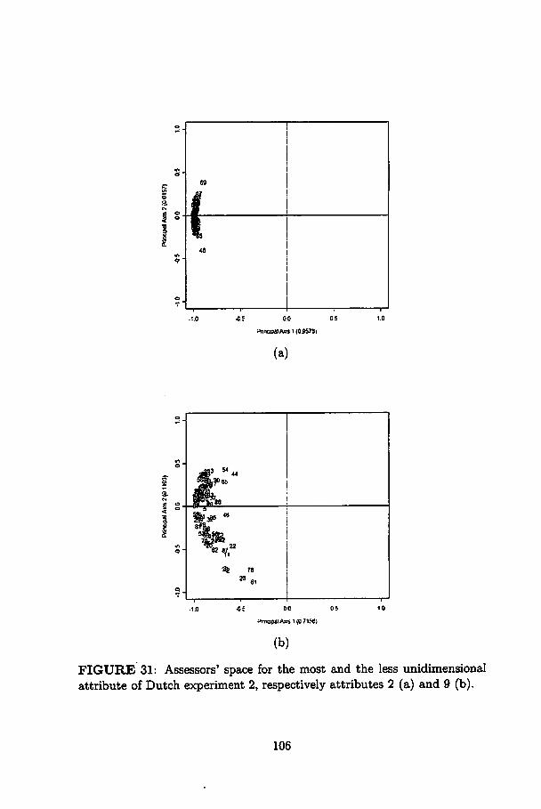
p _ !
•n io "
69
tn
og. flff ICw
S °5 ° •1 % !* |
wv
<?• i1
|
p
7 "' i i : 1—1
0.0 05
PrincipalA« 1 (0S578)
(a)
'*••^ 78
23 «1
45 00 05
SfmoptlAnS1(U7i;<!)
(b)
FIGURE 31: Assessors' space for the most and the less unidimensionalattribute of Dutch experiment 2, respectively attributes 2 (a) and 9 (b).
106
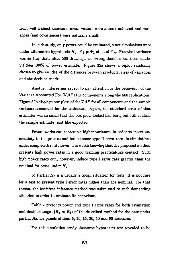
from well trained assessors, mean vectors were almost unbiased and vari-
ances (and covariances) were naturally small.
In such study, only power could be evaluated, since simulations were
under alternative hypothesis H\ : *i ^ #2 # ••• # *n- Practical variance
was so tiny that, affcer 500 drawings, no wrong decision has been made,
yielding 100% of power estimate. Figure 32a shows a biplot randomly
chosen to give an idea of the distances between products, sizes of variances
and the decision made.
Another interesting aspect to pay attention is the behaviour of the
Variance Accounted For (VAF) the components along the 500 replications.
Figure 32b displays box plots of the VAF for ali components and the sample
variance accounted for the estimates. Again, the standard error of that
estimator was so small that the box plots looked like bars, but still contain
the sample estimate, just like expected.
Future works can contemple higher variances in order to insert un-
certainty to the process and induct some type II error rates in simulations
under complete H\. However, it is worth knowing that the proposed method
presents high power rates in a good training practical-like context. Such
high power rates can, however, induce type I error rate greater than the
nominal for cases under Ho.
b) Partia! Hq is a usually a tough situation for tests. It is not rare
for a test to present type I error rates higher than the nominal. For that
reason, the bootstrap inference method was submitted to such demanding
situation in order to evaluate its behaviour.
Table 7 presents power and type I error rates for both estimation
and decision stages (R\ to R&) of the described method for the case under
partial Ho, for paneis of sizes 5, 10, 15, 20, 50 and 90 assessors.
For this simulation study, bootstrap hypothesis test revealed to be
107
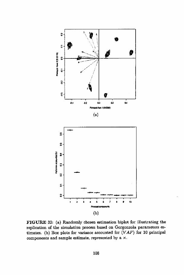
\ \*11 *. *::cj
*
f\ *: """ ,.••"/I
-ii1 .••
1 4j
1— •—• —i"
9i
5
I *
4.4 -02 00 02
PimopalA» 1{0.0288)
(a)
0.4
(b)
FIGURE 32: (a) Randomly chosen estimation biplot for illustrating thereplication of the simulation process based on Gorgonzola parameters es-timates. (b) Box plots for variance accounted for (VAF) for 10 principalcomponents and sample estimate, represented by a x.
108
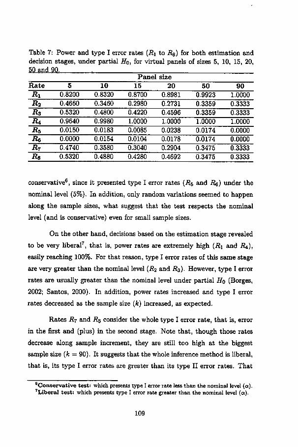
Table 7: Power and type I error rates {Ri to Rs) for both estimation anddecision stages, under partial Ho, for virtual paneis of sizes 5, 10, 15, 20,50 and 90.
Panei size
Rate 5 10 15 20 50 90
Ri 0.8200 0.8320 0.8700 0.8981 0.9923 1.0000
K2 0.4660 0.3460 0.2980 0.2731 0.3359 0.3333
H3 0.5320 0.4800 0.4220 0.4596 0.3359 0.3333
R4 0.9640 0.9980 1.0000 1.0000 1.0000 1.0000
Rs 0.0150 0.0183 0.0085 0.0238 0.0174 0.0000
Re 0.0000 0.0154 0.0104 0.0178 0.0174 0.0000
Rr 0.4740 0.3580 0.3040 0.2904 0.3475 0.3333
Rs 0.5320 0.4880 0.4280 0.4692 0.3475 0.3333
conservative6, since it presented type I error rates (R5 and Rq) under the
nominal levei (5%). In addition, only random variations seemed to happen
along the sample sizes, what suggest that the test respects the nominal
levei (and is conservative) even for small sample sizes.
On the other hand, decisions based on the estimation stage revealed
to be very liberal7, that is, power rates are extremely high (R\ and #4),
easily reaching 100%. For that reason, type I error rates of this same stage
are very greater than the nominal levei (#2 and R$). However, type I error
rates are usually greater than the nominal levei under partial Ho (Borges,
2002; Santos, 2000). In addition, power rates increased and type I error
rates decreased as the sample size (k) increased, as expected.
Rates R7 and R& consider the whole type I error rate, that is, error
in the first and (plus) in the second stage. Note that, though those rates
decrease along sample increment, they are still too high at the biggest
sample size (k = 90). It suggests that the whole inference method is liberal,
that is, its type I error rates are greater than its type II error rates. That
6Conservative test: which presents type I error rate less than the nominal levei (a).7Liberal test: which presents typeI error rate greater than the nominal levei (a).
109
is not a problem itself, since type II error is the worst type or error in most
cases. It is due to the fact that two products are never exactly equal.
However, some attitudes can try to round such problem. If the con
fidence regions were set to higher confidence, more tests will be required, re-
ducing the type I error rate. Further studies must be performed associating
a kind of protection to the confidenceregions. For instance, the Bonferroni
protection, where the confidence are set as 1 - a*, where a* = oc/Cn,2-
Associating estimation and testing stages for decision can be quite
interesting since the prior seems to be liberal and the second, conservative.
Nevertheless, empirical tests (not published) suggest that the bootstrap test
remains conservative even when performed for pair of products that do
not have interception of 95% confidence regions. Therefore, associating
estimation and testing stages enables one to reduce the number of possible
tests (Cn,2) and prevents the whole test to be conservative.
In order to evaluate the stability of the process, the variance ac
counted for principal components, as well as their standard deviations, were
computed along the replications for ali considered sample sizes (Table 8).
Estimates of the variance accounted for were coherent since the smallest
sample size. Standard deviation of such estimates tended to decrease as
the sample size increased, as expected.
Sample size 20 yielded the more discrepant and variable estimates
of the variances accounted for principal components. Such estimates were
taken as randomly diverging from the expected values.
Due to small empirical standard deviations and coherent estimates,
described method was considered efficient to estimate variances accounted
for principal components.
110
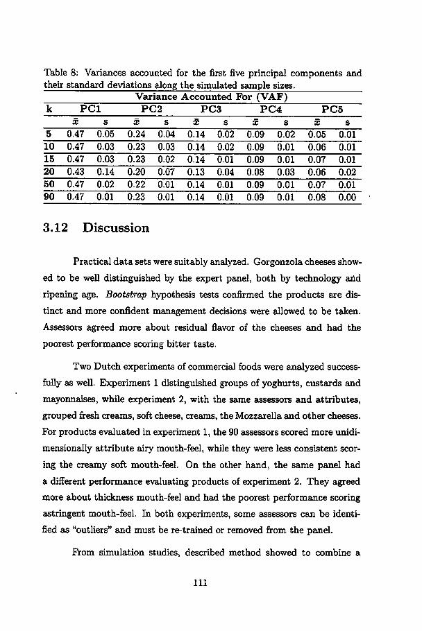
Table 8: Variances accounted for the first five principal components andtheir standard deviations along the simulated sample sizes.
Variance Accounted For (VAF)k PCI PC2 PC3 PC4 PC5
X s X s X s X s X s
5 0.47 0.05 0.24 0.04 0.14 0.02 0.09 0.02 0.05 0.01
10 0.47 0.03 0.23 0.03 0.14 0.02 0.09 0.01 0.06 0.01
15 0.47 0.03 0.23 0.02 0.14 0.01 0.09 0.01 0.07 0.01
20 0.43 0.14 0.20 0.07 0.13 0.04 0.08 0.03 0.06 0.02
50 0.47 0.02 0.22 0.01 0.14 0.01 0.09 0.01 0.07 0.01
90 0.47 0.01 0.23 0.01 0.14 0.01 0.09 0.01 0.08 0.00
3.12 Discussion
Practical data sets were suitably analyzed. Gorgonzola cheeses show-
ed to be well distinguished by the expert panei, both by technology and
ripening age. Bootstrap hypothesis tests confirmed the products are dis-
tinct and more confident management decisions were allowed to be taken.
Assessors agreed more about residual flavor of the cheeses and had the
poorest performance scoring bitter taste.
Two Dutch experiments of commercial foods were analyzed success-
fully as well. Experiment 1 distinguished groups of yoghurts, custards and
mayonnaises, while experiment 2, with the same assessors and attributes,
grouped fresh creams, soft cheese, creams, the Mozzarella and other cheeses.
For products evaluated in experiment 1, the 90 assessors scored more unidi-
mensionally attribute airy mouth-feel, while they were less consistent scor
ing the creamy soft mouth-feel. On the other hand, the same panei had
a different performance evaluating products of experiment 2. They agreed
more about thickness mouth-feel and had the poorest performance scoring
astringent mouth-feel. In both experiments, some assessors can be identi-
fied as "outliers" and must be re-trained or removed from the panei.
From simulation studies, described method showed to combine a
111
liberal first stage (estimation) with a conservative second one (testing), in
the decision process. According to need of protecting against type I or type
II error rates, one can set the confidence of value of the regions suitably
or ever suppress the estimation stage in order to allow more or less tests.
Further works must be done about that issue.
Variances accounted for the principal components were precisely es-
timated, suggesting stability, even in small sample sizes.
One can note a clear behaviour along ali sample sizes: high power
in both estimation and testing stages; high type I error rates in estimation
stage (liberal) and small type I error rates in testing stage (conservative).
Such behaviour seems to be slightly improved along the sample size incre-
ment. However, a protection against the liberality of the estimation stage
might yield better results and keep avoiding testing ali possible combina-
tions of products. Front of those results there is not a clear cut-line for the
sample size, though the big sample, the better. Well trained assessors (less
bias and small variances, as in Gorgonzola experiment) are as important
as big sample sizes. However, the method seems to behave well for expert
paneis and samples sizes greater than 20 to semi-trained people.
For ali cases, the best sample bootstrap resample unit was the whole
matrix. However, when the number of panelists is very small, rows can
be treated as resample units in order to increase the number of possible
virtual paneis, but only in those cases where the variance between assessors
is equivalent to the variance within assessors.
Bootstrap GPA inference routines programmed in R language showed
up to be very computational demanding. For instance, each replication of
the simulation study with 90 assessors, has demanded, in average, 240 hours
(in a Pentium III, 512Mb RAM and Windows operational system). Further
works must be done in order to improve the efficiency of such routines.
112
4 FINAL CONSIDERATIONS
After several studies (simulations, algebraic and practical experi
ments) performed in Procrustes analysis for estimating missing cells and
inferring about the population of focus, it is clear that Procrustes problems
are a rich field to be explored and can contribute greatly to Sensometrics.
Putative values can lead to local minima in missing values estima
tion and therefore must be suitably chosen, for instance setting to zero for
centered matrices. Algorithm efficiency and more suitable constraints also
must be well studied for estimating missing cells. Two-sided eigenvalue
problems with both matrices positive semi-definite seems to be a border
to be passed for a better development of Procrustes problems with general
transformation. As important as such algebraic derivation is the practical
interpretability of such transformation, what can contribute even more with
sensory experiments.
For the first time an inference procedure is described for Procrustes
analysis. However, it has to be discussed and improved both in the esti-
mation/decision process and in the programming efficiency. Optimization
techniques must be used to refine the codes and turn the whole process
lighter. After that, ready-to-use computational packages will be able to
help several sensometricians, statisticians and food engineers world wide
(preferably in open code languages). At least, (another) first step has been
done in order to improve and extend such a classical analysis as Procrustes.
113
APPENDIX A - PROOFS
(A.1): Leat squares estimator ofTunder no restriction is T= íX[Xi J X[X2.Proof: Let
X2 = XxT + e,
where e is a random vector of residuais.1
Then, if e is distributed according to some multivariate distribution
with mean vector $ (vector of zeros) and covariance matrix a2I, and letting
XiT be constant, follows that
E[X2] = E[XiT + e]
= E[XiT\ + E[e]
= XiT.
One estimator of T can be derived by minimizing the residuais sum
of squares in relation to £?[-X*2]:
||*2 - E[X2]\\ = (X2 - E[X2)) {X2 - E[X2))'
= (X2-XiT){X2-XiT)'
= (x2 - XiT) {x'2 - rx{)
= X2X'2 - X2T'X[ - XiTX'2 + XiTT'X[
= f{T)
xIn that case, X\ is a fixed (given) matrix and X2 is random matrix.
114
df{T)dT
= 0
•X[X2 - X[X2 + 2X[X1f = 0 =»
=>2X'lXif = 2X[X2
=*f =(x'iXi)~l x[x2.-1
(A.1)
(A.2):k
Y, \\»i(Xi - H)Qi - sAXi. - lu^Qi, =^^11^(^-1^)^-011i=l
Proof: Let Sí(Xí - lu^Qi = X? and Sí>(Xí> - lu^Qv = X?,. Since
£x; = 5>;,then
E||X?-jrç|| = ELE?-illW-*;)ll2
feEti 11*711 - 2SL EJU^W^) + fcE?=i P?l2
2fc Eti 11*711 - 2EL ELi M*í'*7)2
k k k
kJ2\\xn-Í2Íltr<<xi'xi')t=l t=l i'=l
i<i'
fc / k k y
=*En*"ii-*'- E^E*?i=l \t=l t'=l >
fc fc
=*£wii-£iwii
fc
t=l
= fe E 11**11-EL txj
*EII*"-*1
115
kJ2\\si(Xi-iy?i)Qi-G\\fc=i
(A.2)
(A.3): Eti \MXi - lu^Ti - G\\ = (^EL IM*í - lu})!} - Gi\Proof: From (2.5) and (2.7), yields
1 *
i=l
_T,LiSi{Xi-lu!i)Ti-kGik
E?yjSi'(Xj> - lu^Ty + SjjXj - lu^Tj - kGjk
(fc - l)Gj + Sj(Xi - lu^Tj - kGjk
Si(Xi - lu^Ti - Gi
Using such result,
fc fc
£ \\Si(Xi - 1i4)Tí - G\\ =£ UM* - lti{)r4 - Gi] +(Gi - G)\\i=i t=i
fc
= 5Z hm*< - ^w - G*] - (G - G*)ni=i
=±\\MXi -ufln -Gi] -[«W-y*-Cij
•3)
116
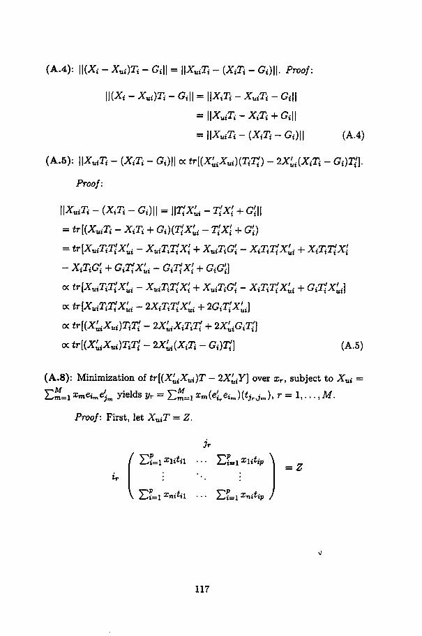
(A.4): \\(Xi - Xui)Ti - Gi\\ = WXuiTi - (XíTí - Gi)\\. Proof:
W(Xi - Xui)Ti - Gi\\ = \\XtTi - XuiTi - GiW
= WXuiTi- XíTí + Gi\\
= \\XviTi-(XiTi-Gi)\\ (A.4)
(A.5): H^T, - {XíTí - Gi)W oc tr [(^«OCnTj) - 2X'ui[XiTi - Gi)T{\.
Proof:
WXuíTí - (XíTí - Gi)\\ = \\liXU - T[X[ + G;||
= tr[(XuiTi - XíTí + Gi^XU - TjAj + G{)
= tr^XviTiTiXui —XuíTíT^Xi + XuíTíGí —XíTíT^X^ + XíTiT^Xi
- XíTíG\ + GiTÍX^ - <?#*{ + GiGW
oc £r[J\UiTiTi.X'Uj —XUiTiTiXi + XujTíGí —XíTíTjX^ + GiTiXui]
oc tr[Xuiri7;,X;i - 2XíTíTIX'uí + 2Gi7í*;i]
oc trK^^JTiTÍ - 2X;íXí7í7;' + 2X^27)
oc tr[(X'uiXUi)TiT; - 2X'vi(XiTi - G<)2j] (A.5)
(A.8): Minimization of ^(A^J^T - 2X'uiY] over sr, subject to Xui -
Em=l «mCim^ yields Vr =EÍL «mC^Cim )(**•>.)» r = 1,. .., M.
Proo/: First, let J\Tuir = Z.
^ EL*ii*ii ... ELxi^p >
\ ^i=l ^nt^tl ••• 2->i=l xniUp /
117
= z
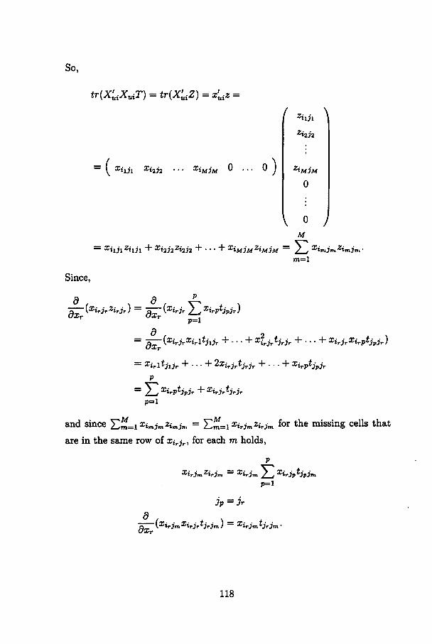
So,
tr(X'uiXuiT) = tr(X'uiZ) = x'uiz =
=( Xhjl X*2J2 '»AfjM 0 ... o
/ *.,. \»U1
ZÍ2J2
Zímjm
0
M
= XixjlZilJl + Xi2J2ZÍ232 + •••+ XÍMJMZÍM3M = 2-*/ Ximjm2imjr
Since,
d
ÕXr\XÍrjrZÍrjr) — Q fotrjr / „X*rpfypjr)
ÕXrp=l
m=l
^ / 2 \= ^"(^Vir^trl^ilJr +•••+Xirjr^jrjr + •••+ XÍrjrXÍrP^jpjr)
= ^iritjxjr + ... + 2a;irjríjrjr + ... + xirptjpjrp
~ / JXirptjpjr + Xirjr*jrjrP=l
and since EÍLi^Wm^imjm = EÍL***»^*» for *he missing cells thatare in the same row of Xirjr, for each m holds,
p
XÍrjmZÍrjm ~ Xirjm / ^Xirjp^jyjm.P=l
Jp — 3r
"n~~\XÍrjmXÍrjr^jrjm) ~ Xirjmhrjr
118
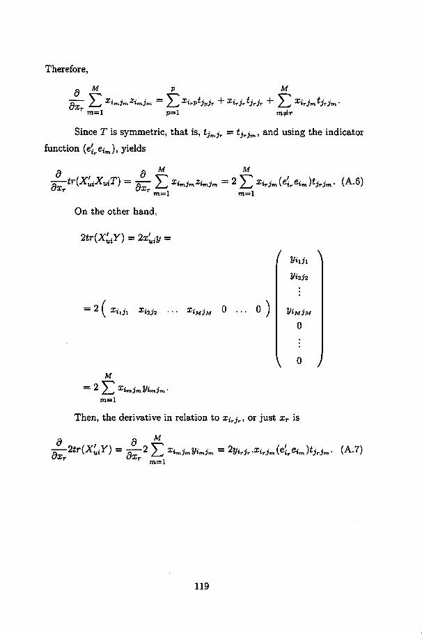
Therefore,
M Md
aT 2^f XWm2Wm —/ „̂ rptjpjr +Xirjrhrjr + 2-*l Xir3rn^jrjrdxT
Since T is symmetric, that is, tjmjr = tjrjm, and using the indicator
function (eíreim), yields
a Õ M M•£—tr(XuiXUiT) = ^— 2^ ximjmzimjm —22^, Zirjm(eírejm)íjrj'm• (A.6)dx da:r
m=l
On the other hand.
2tr(X'uiY) = 2x'uiy =
—2 y xíu! '12.72
M
m=l
Xil\í3M o ... o
3/»2j2
o
V o y
—2 2^ XtTnJm2/tTnJm'm=l
Then, the derivative in relation to Xirjr, or just xr is
Q O Aí
—2ír(X;iy) = —2 5^ ximjmyimjm = 2»*,*. .*<pjm «.c^ )tJrJm. (A.7)r r m=l
119
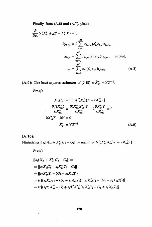
Finally, from (A.6) and (A.7), yields
JLtr(X'uiXUiT-X'uiY) =0M
22/irjr = 2 2_^ Xir3m\eireim)^3rjmm=l
M
m=l
M
2/r = 5Z xm(eíreim)íjrJm. (A.8)m=l
(A.9): The least squares estimator of (2.18) is X^ = YT_1.
Proof:
f(Xrui) = trl(X<XrUi)T-2XtiY}df(XrJ Õ(X<Xrui)T dXfr =
dXL dXL dXL
2XLT - 2Y = 0
Xrui = YT~l (A.9)
kut-
1-1
(A.10):
Minimizing \\sí(Xcí + X^Ti - Gi\\ is minimize tr[(X<X^)T - 2X£Y].
Proof:
Wsi&d + X^Ti-GiW^
= IISiXàTi + síX^Tí - Gi\\
= WsiXZiTi-(Gi-SiXciTi)\\
= ítKsíAÍTí - (Gi - «^TOftsi^r, - (Gi - «i*^))]
= *t[(«í3ÍXS -G'i + síTÍX^SíX^í -Gi + SiXaTi)]
120
V-
= trlsffiXÍXÜTi - SíTÍX<Gí + sfàX&XaTi - siG'iXTuiTi+
+ GíGí - SiGiXãTi + SiTlX^X^iTi - síT^X^Gí + s^TlX^XãTi]
From now on, lets consider only those term that depend on X^,
since minimizing them is minimizing the whole expression.
oc ír[Sj7iXuiXuiTi —síTiXuiGi + SíT^X^XcíTí —SíG^XuíTí + SíT^X^X^Tí]
= tr^X^X^Tl + 2s2iX<XciTiTl - 2siX^iGiT'i\
= trlsUX^X^TiXl - 2síX<(Gí - SiX^T-)^]
= trl(X<XruJTiT! - 2XT2s;lGi - XtTtfR
= trl(X<Xrui)T-2XtiY}. (A.10)
(A.11): Ti = ^(X^X^X^Gi.
Proof:
f(Ti) = WsiXciTi-Gi\\
= tr [(siXaTi - Gi)'(siXciTi - G{)]
= tr [(síTIX^ - G^SiXaTi - Gi)]
= tr [síT-XciXcíTí - síT^X^Gí - SiGiXãTi - GjGi]
= tr [slTlX^XaTi - 2siTlX'ciGi - G^d]
g/P» = QdTi
-25^^ + 25^X^ = 0
SiXçid = SiXçiXçiTi
ti = -(X^Xa^X^Gi (A.11)Si
121
(A.12): EL 11**5^ " «PMH = s'(kDiag(S) - S)s
Proof:
k
53115^^-5^*^11 =
k
-kJ^WsiXcW-GWi=l
fc
= fc 53 tr^TlX^XàTi - 2síT;X'*G +G'G)i=i
fc fc fc
= fc 53s\trVÍX5X^Ti) - 2fc53 SitrtfXZG) +fc53 tr(G'G)i=\ t=i i=i
fc fc / fc \
=fc 53 5?tr(7p^*^) - 253 5iír (tíx* 53 *,*s,3;,) +
53 svXtfli* J (53 Si'Xc\>Ti't'=l / Vsl
fc fc
= fc 53sjtHTiX^X^Ti) - 25353wtr(2ÍX5XS,2V)+i=l t=
fc fc
i=l i'=l
fc fc
= fc53 fapiXSXàTi) - 5353«,a</ír(2íJCS^i^)i=l i=l i'=l
fc fc
= 53[fc5?ír(7?X;-*dri) - 53wtrPiXSXà.Te)]
i=l t'=l
+ tr
t=l i'=l
fc fc
i=i í'=l
fc fc
= 53l(fc - i^mtíxZxiPí) - 535i5i,ír(^XSX-,riO]i=i iV»
122
fc
=s2(k - l)ír(7íJCS^ri) - 5] navtrfâXZXàTi.) + ...i'jíl
k
+ s2k(k - l)tr(TÍX'ckX*ckTk) - 53 8k8i.trÇríXcíXàTi')i'jík
= s'(kDiag(S) - S)s (A.12)
ía i3V (x - x)2 , (y - v)2 2(* - s)(y - ?) < v2 ^^ °;- deí(C)/52 +det(C)/sl det(C)/sxy ~XaK)
Proof:
(z-n)'Y.-l(z-tx)^X2{2)
X~IH \ í cri axy \ í x-fixy-Vy) \°xy o% ) \ y- My
1 I X-px \ I °l -°xy \ í x- Px i 2
I f
J. I X X \ \ Sy ~SXy i / X — X
det(C) \ y-y I \ -Sxy s2x J \y-y
~XÍ(2)
~ xS(2)
•j^êjfr - x?s2y +(y - y)2s2x - 2(x - x)(y - y)sxy <j£(2)(*-*)2 + (y-y)2 _2(*-g)(y-fl <y2(2) (A 13)
deí(C)/52 + deí(C)/52 det(C)/sxy ~Xq^} ^ló)
123
APPENDIX B - R FUNCTIONS
Main R functions used along the thesis are briefly described below.
R codes are not published because the need of optimization in performance,
but they will be turn public as soon as such improvements occur.
• bootGPA.cr (X, ortho=TRUE, sf=TRUE, resmpl=100, conf=0.95)
Performs generalised (or ordinary) Procrustes analysis and builds 1-
a bootstrap confidence regions for ali evaluated objects. It allows
orthogonal or general transformations, with or without scaling and
enables the user to set the resample size and the confidence of the
region.
• bootGPA.tst (X, a, b, resmpl=500, plot.result=TRUE)
Performs generalised (or ordinary) Procrustes analysis and a a boot
strap test between two products a and b (Ho : a = 6). It allows an
empirical histogram to be constructed and the empirical p-value is
shown on the console output.
• missingGPA (X, ortho = TRUE, sf = TRUE, tol = le-4, plotresult
= FALSE, plotiterat = FALSE)
Performs iteratively generalised (or ordinary) Procrustes adjustment
and missing cells estimation (estimation/minimisation). It allows or
thogonal or general transformations, with or without scaling, enable
124
the user to set the convergence tolerance, and plot either the GPA
biplot or the residual sum of squares convergence through iterations.
• histMv (a, boot= TRUE, levei = .95, ellip = FALSE, point = FALSE,
pty = 20, xn=c("X"), yn=c("Y"))
Builds bivariate histograms for data sets form both bootstrapping or
not. The confidence can be set. An ellipse can be draw on the plot
if desired. The original points can be draw or not and the character
can be chosen, as well as the labels of the axes.
• bootGPA (X, attrib = c(seq(l:dim(X)[2])), ortho = TRUE, sf= TRUE,
resmpl = 100, conf = 0.95, rows = FALSE, plotresult = TRUE)
Performs generalised (or ordinary) Procrustes analysis and the whole
described inference procedure. It allows orthogonal or general trans
formations, with or without scaling and enables the user to set the
resample size, the confidence of the region, if rows must be the re
sample units, and draws the final biplot with original attributes.
• p.cons (X, attrib=seq(l:dim(X)[2j), plotpr=FALSE, plotas=FALSE,
scree=FALSE, bar. C=TRUE)
Performs Dijksterhuis' panei consonance test. It plots either product
space, assessors space, scree plot or the bar plot of statistic C, with
original attribute labels.
125

REFERENCES
AGUIAR, R. L. Produção e caracterização de massa de pizzapré-assada e congelada. 1995. 88 p. Dissertação (Mestrado em Giênciados Alimentos) - Universidade Federal de Viçosa, Viçosa.
AKGA, M. D. Generalized procrustes analysis and its applicationsin photogrammetry. 2003. 23 p. Zurich: Swiss Federal Instituteof Technology, Institute of Geodesy and Photogrammetry, ETH-Hoenggerberg. Disponível em: <http://e-coUection.ethbib.ethz.cn/ecol-pool/bericht/bericht_363.pdf>. Acesso em: 28 out. 2004.
ALLCROFT, D. J.; GLASBEY, C.A.; PAULO, M. J. A latentgaussian model for multivariate consumption data. Food Quality andPreference, Cidade, v. 3, n. 18, p. 508-516, 2007.
AMERINE, M. A.; PANGBORN, R. M.; ROESSLER, E. B. Principiesof sensory evaluation of food. 1. ed. San Francisco: Academic Press,1965. 602 p.
ANZALDUA-MORALES, A. La evaluación sensorial de losalimentos en Ia teoria y Ia práctica. Zaragoza: Editorial Acribia S.A.,1994. 198 p.
AQUINO, A. A. Aproveitamento do tegumento da semente docacau em ração para coelhos em crescimento. 1992. 59p. Dissertação(Mestrado em Zootecnia) - Universidade Federal de Viçosa, Viçosa.
ASTRUC, C.; BLUMENTHAL, D.; DELARUE, J.; DANZART, M.;SIEFFERMANN, J. M. How to construct a global driving procedure fordynamic hedonic tests? In: THE SENSOMETRICS MEETING, 8., 2006,As, Norway. Proceedings..., 2006. p. 24.
BORGES, L.C. Poder e taxas de erro tipo I dos testes Scott-Knott,Tukey e Student-Newman-Keuls sob distribuições Normal enão Normais dos resíduos. 2002. 94 p. Dissertação (Mestrado emEstatística e Experimentação Agropecuária) - Universidade Federal deLavras, Lavras.
126
CARDOSO, R. L. Estabilidade de geléia de jambo-vermelho(Eugenia malaccensis, Lin) em copo de vidro. 1994. 157 p.Dissertação (Mestrado em Ciência dos Alimentos) - Universidade Estadualde Campinas, Campinas.
CHAGAS, S. J. R. Caracterização química e qualitativa de caféde alguns municípios de três regiões produtoras de MinasGerais. 1994. 83 p. Dissertação (Mestrado em Ciência dos Alimentos) -Universidade Federal de Lavras, Lavras.
CHREA, C; VALENTIN, D.; SULMONT-ROSSÉ, C; LY MAI, H.;HOANG NGUYEN, D.; ABDI, H. Culture and odor categorization:agreement between cultures depends upon the odors. Food Quality andPreference, Cidade, v. 7-8, n. 15. p. 669-679, 2004.
CLIFF, N. Orthogonal rotation to congruence. Psychometrika, Cidade,v. 31, p. 33-42, 1966.
COMMANDEUR, J. J. F. Matching configuraiions. Leiden: DSWOPress, 1991. 171 p.
DACHS, J. N. W. Estatística computacional: uma introdução emTurbo Pascal. Rio de Janeiro: LTC, 1988. paginas p.
DAEMS, V.; DELVAUX, F. Multivariate analysis of descriptive sensorydata on 40 commercial beers. Food Quality and Preference, Cidade,v. 5-6, n. 8, p. 373-380, 1997.
DAIROU, V.; SIEFFERMANN, J.; PRIEZ, A.; DANZART,M. Sensory evaluation of car brake systems - the useof flash profile as a preliminary study before a con-vention profile. Disponível em: <http://www.perception-sensorieUe.com/Congress2003/Dairou_SAE.pdf>. Acesso em: 2 ago.2004.
DEMPSTER, A.P.; LAIRD, N.M.; RUBIN, D.B. Maximum likelihoodfrom incomplete data via the em algorithm (with discussion). Journal ofRoyal Statistical Society B, v. 39, p. 1-38, 1977.
DIJKSTERHUIS, G. Assessing panei consonance. Food Quality andPreference, v. 6, p. 7-14, 1995.
DRYDEN, I. L.; MARDIA, K. V. Statistical Shape Analysis.Chichester: John Wiley, 1998. 376 p.
127
EFRON, B. Bootstrap methods: Another look at the jackknife. Annalsof Statistics, v. 7, p. 1-26, 1979.
EFRON, B.; TIBSHIRANI, R. An introduction to the bootstrap.New York: Chapman k Hall, 1993. 311 p.
FERREIRA, E. B. Análise Generalizada de Procrustes via R:Uma aplicação em laticínios. 2004. 216 p. Dissertação (Mestrado emEstatística e Experimentação Agropecuária) - Universidade Federal deLavras, Lavras.
FERREIRA, E.B.; MAGALHÃES, F.A.R.; OLIVEIRA, M.S.;FERREIRA, D.F. Sensory profile of the gorgonzola type cheese throughbootstrap confidence regions in generalized procrustes analysis. Revistado Instituto de Laticínios Cândido Tostes, v. 62, p. 535-540, 2007.
GOWER, J. C. Statistical methods for comparing different multivariateanalysis of the same data. In: HODSON, J.R.; KENDALL, D.G.; TAUTU,P. Mathematics in the Archaeological and Historical Sciences.Edinburgh: Edinburgh University Press, 1971. p. 138-149.
GOWER. J. C. Generalised procrustes analysis. Psychometrika, v. 1, n.40, p. 33-51, 1975.
GOWER, J. C; DIJKSTERHUIS, G. B. Procrustes Problems. Oxford:Oxford University Press, 2004. 256 p.
GREEN, B. F. The orthogonal approximation of an oblique structure infactor analysis. Psychometrika, v. 17, p. 429-440, 1952.
HALL, P. The bootstrap and edgeworth expansions. New York:Springer-Verlag, 1992. paginas.
HEYMANN, H. Sensory science and sensometrics: yesterday, today andtomorrow. In: THE SENSOMETRICS MEETING, 8., 2006, Ás, Norway.Proceedings... 2006. p. 2.
HUMMER, S. Application of multivariate analysis of variance. FoodQuality and Preference, v. 3, n. 9, p. 83-85, 1998.
HURLEY, J. R.; CATTLE, R. B. The procrustes program: producingdirect rotation to test a hypothesized factor structure. BehavioralScience, v. 7, p. 258-262, 1962.
128
HUSSON, F.; LÊ, S.; PAGÈS, J. Confidence ellipse for the sensoryprofiles obtained by principal component analysis. Food Quality andPreference, v. 16, p. 245-250, 2005.
JOHNSON, R.A.; WICHERN, D.W. Applied multivariate statisticalanalysis. 4. ed. New Jersey: Prentice Hall, 1998. 816 p.
JORGE, N. Curvas de secagem de cogumelo (Agaricus bisporus)e avaliação sensorial do produto após diferentes períodos dearmazenagem. 1989. 80 p. Dissertação (Mestrado em Ciência dosAlimentos) - Universidade Federal de Viçosa, Viçosa.
KRISTOF, W.; WINGERSKY, B. Generalization of the orthogonalprocrustes rotation procedure for more than two matrices. Proceedingsof the 79th Annual Convention of the American PsychologicalAssociation, v. 6, p. 89-90, 1971.
LELE, S. R.; RICHTSMEIER, J. T. An invariant approach to theStatistical Analysis of Shape. Boca Raton: Chapman and Hall, 2001.paginas.
LINGOES, J. C; BORG, I. Alternative measures of fit for theschõnemann-carroll matrix fitting algorithm. Psychometrika, v. 43, p.423-427, 1978.
MACDOUGALL, D. B. Coloring of food, drugs, and cosmetics. FoodQuality and Preference, v. 3, n. 11, p. 255, 2000.
MAGALHÃES, F. A. R. Estudo sobre a evolução de parâmetrosfísicoquímicos e sensoriais durante a maturação do queijo tipogorgonzola. 2002. 88 p. Tese (Doutorado em Ciência dos Alimentos) -Universidade Federal de Lavras, Lavras.
MALVINO MADRID, R. M. Efeito da salinidade da água demar e da alimentação na composição de solutos muscularese de algumas propriedades sensoriais do camarão de águadoce, Macrobrachium rosenbergii (De Man, 1879) (CrustáceaPalaemonidae). 1994. 191 p. Dissertação (Mestrado em Ciência dosAlimentos) - Universidade Estadual de Campinas, Campinas.
MANLY, B. F. J. Randomization, bootstrap and Monte Cariomethods in biology. 2. ed, London: Chapman & Hall, 1998. 399 p.
129

MIRANDA, V. F. L. Avaliação Monte Cario de testes assintóticos ede Bootstrap para autocorrelação residual. 2004. 77 p. Dissertação(Mestrado em Estatística e Experimentação Agropecuária) - UniversidadeFederal de Lavras, Lavras.
MIRONOV, A.; PEVZNER, P.; GELFAND, M. Procrustes:Gene recognition via spliced alignment. 2004. Disponível em:<http://www.hto.usc.edU/software/procrustes/index.html#salign>.Acesso em: 29 fev. 2004.
MORAES, D. A. A morfometria geométrica e a 'revolução na mor-fo met ria': localizando e visualizando mudanças na forma dos organismo. 2004. Disponível em: <http://www.bioletim.hpg.ig.com.br/III-3/Artigos/moraes.htm>. Acesso em: 17 fev. 2004.
MUELLER, C. G. Psicologia sensorial. Rio de Janeiro: Zagar Editores,1966. 177 p.
NORONHA, J. F. Apontamentos de análise sensorial. Coimbra: ESAC, 2003. Disponível em:<http://pwp.netcabo.pt/0331491102/A.S/Apontamentos%5
Csebenta_v_l_0.pdf>. Acesso em: 2 ago. 2004.
0'MAHONY, M. Sensory evaluation of food. New York: MareeiDekker, Ico., 1985. 487 p.
PEAY, E. R. Multidimensional rotation and scaling of configurations tooptimal agreement. Psychometrika, v. 53, p. 199-208, 1988.
R DEVELOPMENT CORE TEAM, version 2.6.0: R: A Language andEnvironment for Statistical Computing. R Foundation for StatisticalComputing, Vienna. 2007.
RANGARAJAN, A.; CHUI, H.; BOOKSTEIN, F. L. Thesoftassign matching algorithm. 2003. Disponível em:<http://citeseer.nj.nec.com/rangarajan97softassign.html>. Acessoem: 18 dez. 2004.
RODRIGUES, L. A.; SANTOS, V. F. Morfometria geométrica -aplicações em paleobiologia de Dinossauros. 2004. Disponível em:<http://www.mnhn.ul.pt/dinos/public_html/Luis_AJElodrigues/
ABstractCONGGEo.htm>. Acesso em: 17 fev. 2004.
130
SANTOS, C. dos. Novas alternativas de testes de agrupamentoavaliadas por meio de simulação Monte Cario. 2000. 85 p.Dissertação (Mestrado em. Estatística e Experimentação Agropecuária) -Universidade Federal de Lavras, Lavras.
SCHONEMANN, P. H. A generaUzed solution of the orthogonal procrustesproblem. Psychometrika, v. 1, n. 31, p. 1-10, 1966.
SCHONEMANN, P. H.; CARROL, R. M. Fitting one matrix to anotherunder choice of a central dilation and a rigid motion. Psychometrika, v.3, n. 35, p. 245-256, 1970.
SINESIO, F.; MONETA, E.; SABÁ, A. Comparison of multivariatemethods of analysis to evaluate panelists' performance. Food Qualityand Preference, v. 4, n. 3, p. 201-208, 1991-1992.
TEN BERGE, J. M. F. Orthogonal procrustes rotation for two or morematrices. Psychometrika, v. 42, p. 267-276, 1977.
TEN BERGE, J. M. F.; KNOL, D. L. Orthogonal rotations tomaximal agreement for two or more matrices of different column orders.Psychometrika, v. 49, p. 49-55, 1984.
THYBO, A. K.; MARTENS, M. Analysis of sensory assessors in textureprofiling of potatoes by multivariate modeling. Food Quality andPreference, v. 4, n. 11, p. 283-288, 2000.
WILLIAMS, A. A.; LANGRON, S. P. The use of free choice profilingfor the evaluation of commercial ports. Journal of Science and FoodAgriculture, v. 5, n. 35, p. 558-568, 1984.
WORTEL, V. A. L.; WIECHERS, J. W. Skin sensory performance ofindividual personal care ingredients and marketed personal care products.Food Quality and Preference, v. 1-2, n. 11, p. 121-127, 2000.
131
Top Related