HOW TO GUIDE

Solar collectors and photovoltaics

in energyPRO

© Copyright and publisher:

EMD International A/S

Niels Jernes vej 10

9220 Aalborg Ø

Denmark

Phone: +45 9635 44444

e-mail: emd@emd.dk

web: www.emd.dk

EMD International A/S, June 2016

About energyPRO

energyPRO is a Windows-based modeling software package for combined techno-economic

analysis and optimisation of complex energy projects with a combined supply of electricity and thermal energy from multiple different energy producing units.

The unique programming in energyPRO optimises the operations of the plant including energy

storage (heat, fuel, cold and electrical storages) against technical and financial parameters

to provide a detailed specification for the provision of the defined energy demands, including heating, cooling and electricity use.

energyPRO also provides the user with a detailed financial plan in a standard format approved

by international banks and funding institutions. The software enables the user to calculate

and produce a report of the emissions by the proposed project.

energyPRO is very user-friendly and is the most advanced and flexible software package for making a combined technical and economic analysis of multi-dimensional energy projects.

For further information concerning the applications of energyPRO please visit www.emd.dk.

Terms of application

EMD has made every attempt to ensure the accuracy and reliability of the information

provided in this Guide. However, the information is provided "as is" without warranty of any

kind. EMD does not accept any responsibility or liability for the accuracy, content, completeness, legality, or reliability of the information contained in this guide.

No warranties, promises and/or representations of any kind, expressed or implied, are given

as to the nature, standard, accuracy or otherwise of the information provided in this guide

nor to the suitability or otherwise of the information to your particular circumstances. In no

event shall EMD be liable for any loss or damage of whatever nature (direct, indirect,

consequential, or other) whether arising in contract, tort or otherwise, which may arise as a

result of your use of (or inability to use) this guide, or from your use of (or failure to use) the information in this guide.

Page | 5

Contents

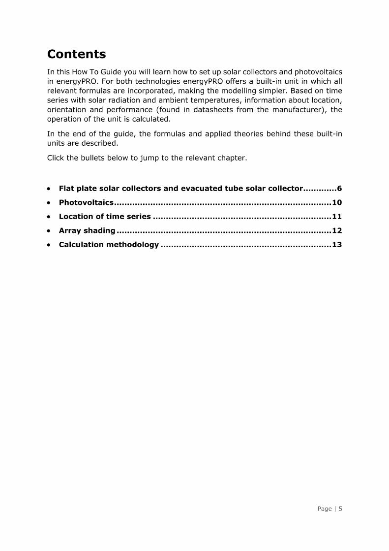
In this How To Guide you will learn how to set up solar collectors and photovoltaics

in energyPRO. For both technologies energyPRO offers a built-in unit in which all

relevant formulas are incorporated, making the modelling simpler. Based on time

series with solar radiation and ambient temperatures, information about location,

orientation and performance (found in datasheets from the manufacturer), the

operation of the unit is calculated.

In the end of the guide, the formulas and applied theories behind these built-in

units are described.

Click the bullets below to jump to the relevant chapter.

Flat plate solar collectors and evacuated tube solar collector ............. 6

Photovoltaics .................................................................................... 10

Location of time series ..................................................................... 11

Array shading ................................................................................... 12

Calculation methodology .................................................................. 13

Page | 6

Flat plate solar collectors and evacuated

tube solar collector

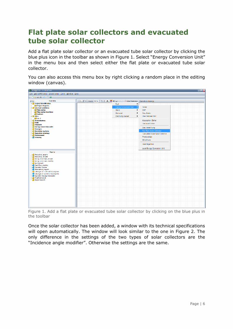
Add a flat plate solar collector or an evacuated tube solar collector by clicking the

blue plus icon in the toolbar as shown in Figure 1. Select “Energy Conversion Unit”

in the menu box and then select either the flat plate or evacuated tube solar

collector.

You can also access this menu box by right clicking a random place in the editing

window (canvas).

Figure 1. Add a flat plate or evacuated tube solar collector by clicking on the blue plus in

the toolbar

Once the solar collector has been added, a window with its technical specifications

will open automatically. The window will look similar to the one in Figure 2. The

only difference in the settings of the two types of solar collectors are the

“Incidence angle modifier”. Otherwise the settings are the same.

Page | 7

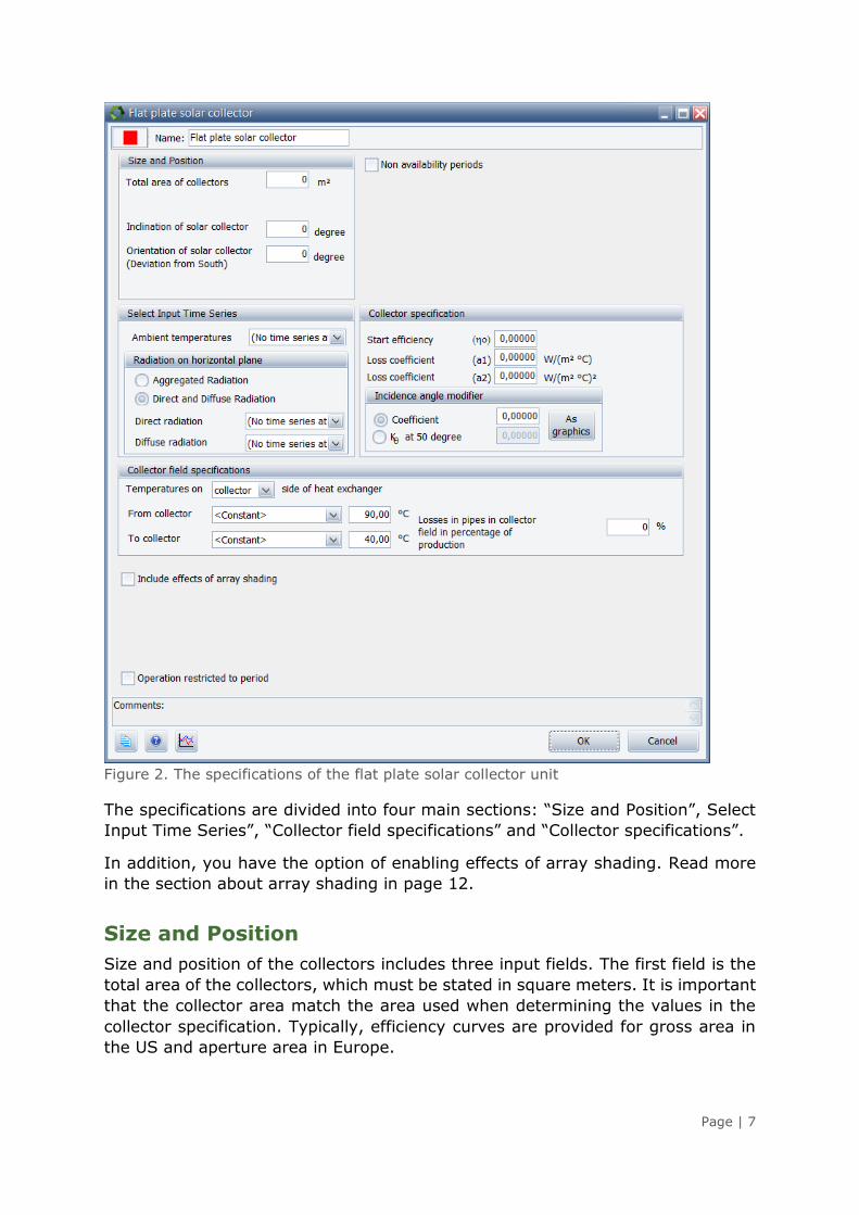
Figure 2. The specifications of the flat plate solar collector unit

The specifications are divided into four main sections: “Size and Position”, Select

Input Time Series”, “Collector field specifications” and “Collector specifications”.

In addition, you have the option of enabling effects of array shading. Read more

in the section about array shading in page 12.

Size and Position

Size and position of the collectors includes three input fields. The first field is the

total area of the collectors, which must be stated in square meters. It is important

that the collector area match the area used when determining the values in the

collector specification. Typically, efficiency curves are provided for gross area in

the US and aperture area in Europe.

Page | 8

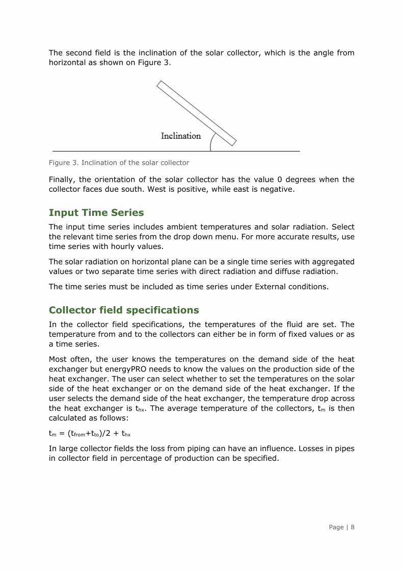
The second field is the inclination of the solar collector, which is the angle from

horizontal as shown on Figure 3.

Figure 3. Inclination of the solar collector

Finally, the orientation of the solar collector has the value 0 degrees when the

collector faces due south. West is positive, while east is negative.

Input Time Series

The input time series includes ambient temperatures and solar radiation. Select

the relevant time series from the drop down menu. For more accurate results, use

time series with hourly values.

The solar radiation on horizontal plane can be a single time series with aggregated

values or two separate time series with direct radiation and diffuse radiation.

The time series must be included as time series under External conditions.

Collector field specifications

In the collector field specifications, the temperatures of the fluid are set. The

temperature from and to the collectors can either be in form of fixed values or as

a time series.

Most often, the user knows the temperatures on the demand side of the heat

exchanger but energyPRO needs to know the values on the production side of the

heat exchanger. The user can select whether to set the temperatures on the solar

side of the heat exchanger or on the demand side of the heat exchanger. If the

user selects the demand side of the heat exchanger, the temperature drop across

the heat exchanger is thx. The average temperature of the collectors, tm is then

calculated as follows:

tm = (tfrom+tto)/2 + thx

In large collector fields the loss from piping can have an influence. Losses in pipes

in collector field in percentage of production can be specified.

Page | 9

Collector specification

Information regarding the collector specifications has to be delivered by the

manufacture of the collectors. For more information about the start efficiency and

loss coefficients, please refer to page 23 in Calculation methodology.

For the flat plate solar collector, the incidence angle modifier can either be defined

as a coefficient or as its value at an incidence angle of 50 degrees. In both cases

the resulting incidence angle modifier (IAM) can be seen graphically.

For the evacuated tube solar collector, the input to the incidence angle modifier

looks like on Figure 4.

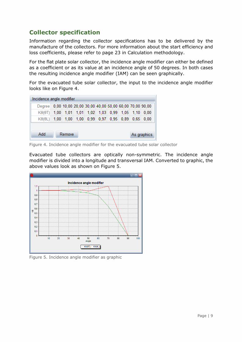
Figure 4. Incidence angle modifier for the evacuated tube solar collector

Evacuated tube collectors are optically non-symmetric. The incidence angle

modifier is divided into a longitude and transversal IAM. Converted to graphic, the

above values look as shown on Figure 5.

Figure 5. Incidence angle modifier as graphic

Page | 10

Photovoltaics

As with the solar collector, add a PV-unit by clicking the blue plus icon as shown

in Figure 1 and select the Photovoltaic in the Energy Conversion Unit menu.

Once added, double-click the unit to open its specification window like the one

shown in Figure 6.

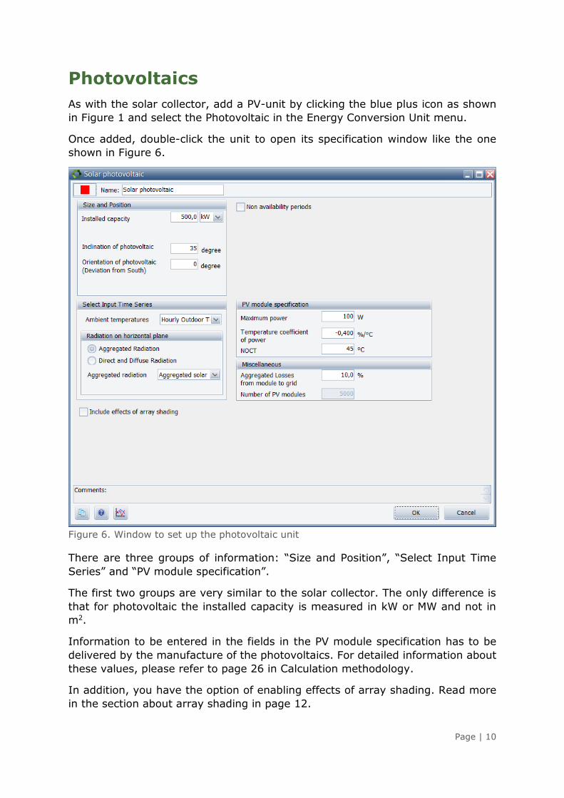
Figure 6. Window to set up the photovoltaic unit

There are three groups of information: “Size and Position”, “Select Input Time

Series” and “PV module specification”.

The first two groups are very similar to the solar collector. The only difference is

that for photovoltaic the installed capacity is measured in kW or MW and not in

m2.

Information to be entered in the fields in the PV module specification has to be

delivered by the manufacture of the photovoltaics. For detailed information about

these values, please refer to page 26 in Calculation methodology.

In addition, you have the option of enabling effects of array shading. Read more

in the section about array shading in page 12.

Page | 11

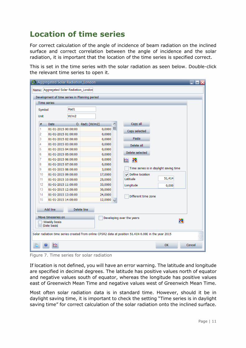
Location of time series

For correct calculation of the angle of incidence of beam radiation on the inclined

surface and correct correlation between the angle of incidence and the solar

radiation, it is important that the location of the time series is specified correct.

This is set in the time series with the solar radiation as seen below. Double-click

the relevant time series to open it.

Figure 7. Time series for solar radiation

If location is not defined, you will have an error warning. The latitude and longitude

are specified in decimal degrees. The latitude has positive values north of equator

and negative values south of equator, whereas the longitude has positive values

east of Greenwich Mean Time and negative values west of Greenwich Mean Time.

Most often solar radiation data is in standard time. However, should it be in

daylight saving time, it is important to check the setting “Time series is in daylight

saving time” for correct calculation of the solar radiation onto the inclined surface.

Page | 12

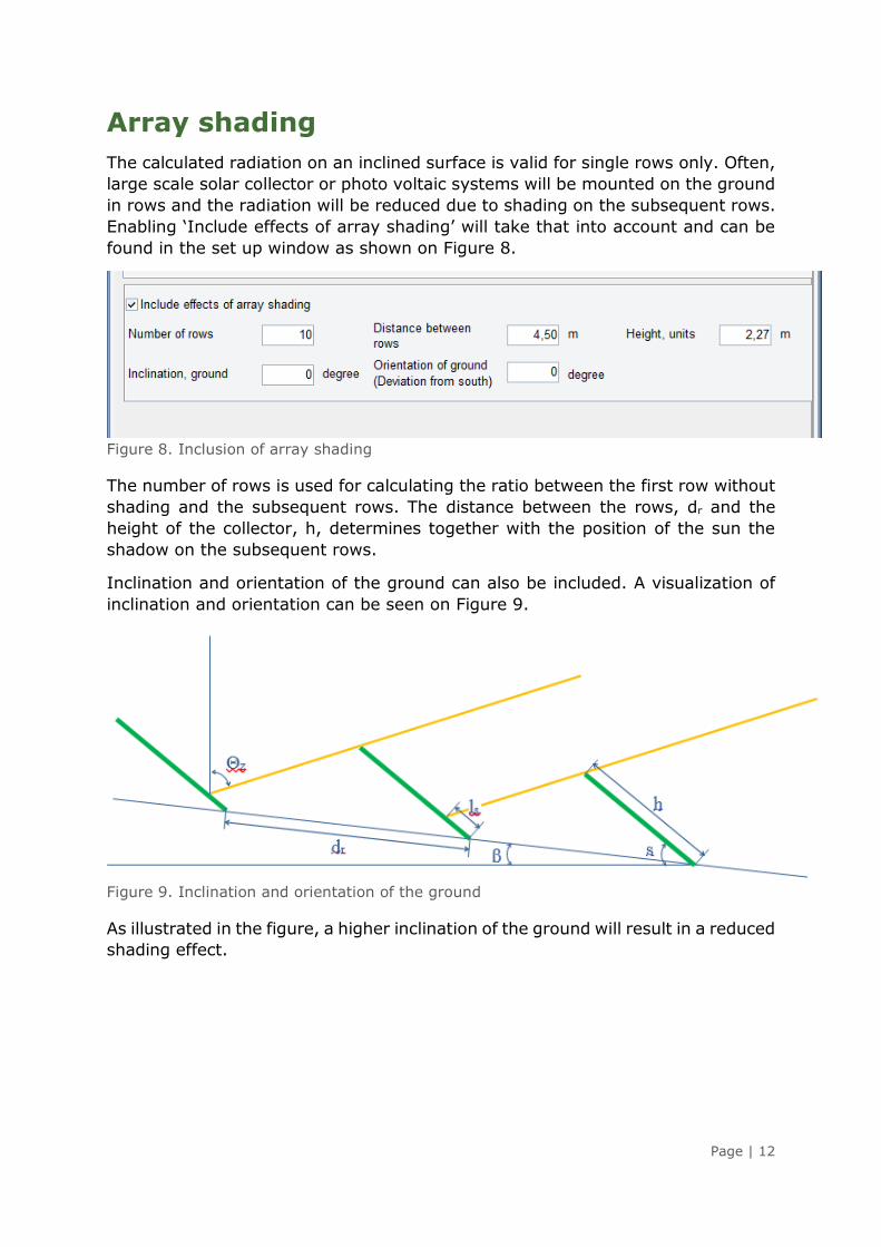
Array shading

The calculated radiation on an inclined surface is valid for single rows only. Often,

large scale solar collector or photo voltaic systems will be mounted on the ground

in rows and the radiation will be reduced due to shading on the subsequent rows.

Enabling ‘Include effects of array shading’ will take that into account and can be

found in the set up window as shown on Figure 8.

Figure 8. Inclusion of array shading

The number of rows is used for calculating the ratio between the first row without

shading and the subsequent rows. The distance between the rows, dr and the

height of the collector, h, determines together with the position of the sun the

shadow on the subsequent rows.

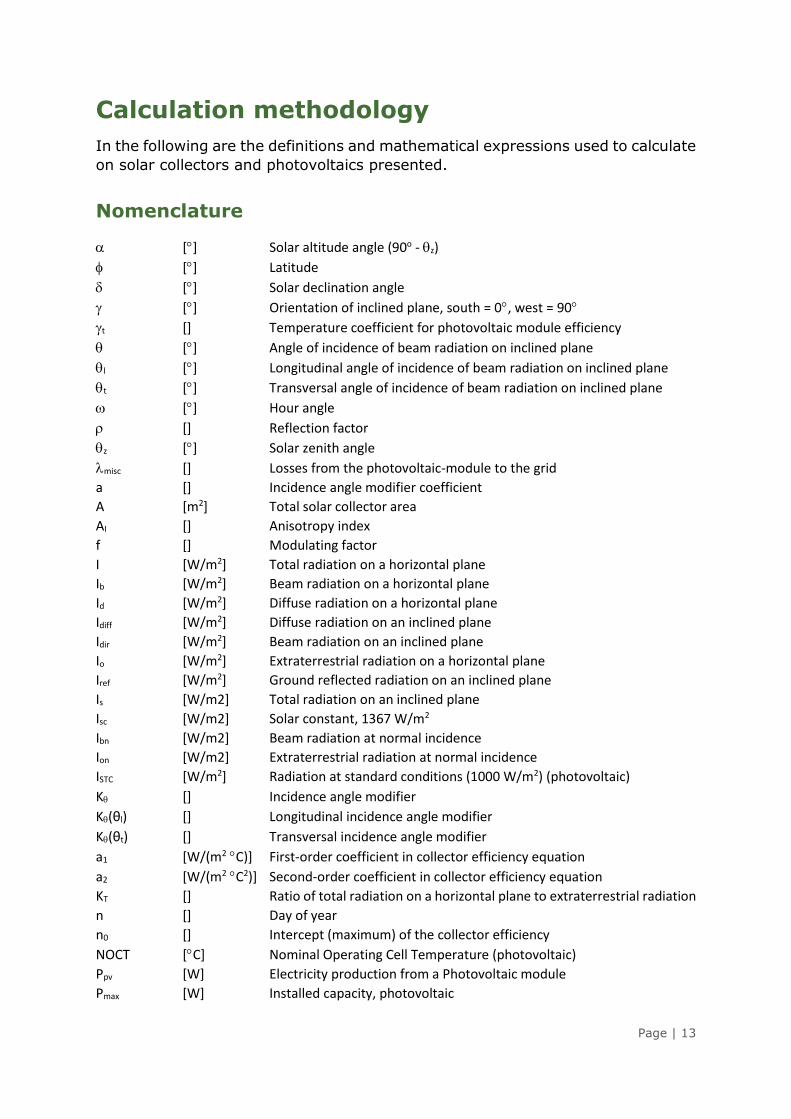
Inclination and orientation of the ground can also be included. A visualization of

inclination and orientation can be seen on Figure 9.

Figure 9. Inclination and orientation of the ground

As illustrated in the figure, a higher inclination of the ground will result in a reduced

shading effect.

Page | 13

Calculation methodology

In the following are the definitions and mathematical expressions used to calculate

on solar collectors and photovoltaics presented.

Nomenclature

[] Solar altitude angle (90o - z)

[] Latitude

[] Solar declination angle

[] Orientation of inclined plane, south = 0, west = 90

t [] Temperature coefficient for photovoltaic module efficiency

[] Angle of incidence of beam radiation on inclined plane

l [] Longitudinal angle of incidence of beam radiation on inclined plane

t [] Transversal angle of incidence of beam radiation on inclined plane

[] Hour angle

[] Reflection factor

z [] Solar zenith angle

misc [] Losses from the photovoltaic-module to the grid

a [] Incidence angle modifier coefficient

A [m2] Total solar collector area

AI [] Anisotropy index

f [] Modulating factor

I [W/m2] Total radiation on a horizontal plane

Ib [W/m2] Beam radiation on a horizontal plane

Id [W/m2] Diffuse radiation on a horizontal plane

Idiff [W/m2] Diffuse radiation on an inclined plane

Idir [W/m2] Beam radiation on an inclined plane

Io [W/m2] Extraterrestrial radiation on a horizontal plane

Iref [W/m2] Ground reflected radiation on an inclined plane

Is [W/m2] Total radiation on an inclined plane

Isc [W/m2] Solar constant, 1367 W/m2

Ibn [W/m2] Beam radiation at normal incidence

Ion [W/m2] Extraterrestrial radiation at normal incidence

ISTC [W/m2] Radiation at standard conditions (1000 W/m2) (photovoltaic)

K [] Incidence angle modifier

K(θl) [] Longitudinal incidence angle modifier

K(θt) [] Transversal incidence angle modifier

a1 [W/(m2 C)] First-order coefficient in collector efficiency equation

a2 [W/(m2 C2)] Second-order coefficient in collector efficiency equation

KT [] Ratio of total radiation on a horizontal plane to extraterrestrial radiation

n [] Day of year

n0 [] Intercept (maximum) of the collector efficiency

NOCT [C] Nominal Operating Cell Temperature (photovoltaic)

Ppv [W] Electricity production from a Photovoltaic module

Pmax [W] Installed capacity, photovoltaic

Page | 14

Pelec [W] Electricity production to the grid from the photovoltaic plant

Rb [] Ratio of beam radiation on an inclined plane to beam on horizontal

Rd [] Ratio of diffuse radiation on an inclined plane to diffuse on horizontal

Rr [] Ratio of reflected radiation on an inclined plane to total radiation on

horizontal level

s [] Inclination of surface

ta [C] Ambient temperature

tm [C] Solar collectors average temperature

Tcell [C] Photovoltaic operation cell temperature

TSTC [C] Cell temperature at standard conditions (25 C) (photovoltaic)

TTST h] True Solar Time

Tz [h] Zone time or local time

Tj [h] Equation of time

K [] Local Constant

CorDST [h] Correction for daylight saving time

External conditions

In energyPRO external time series are needed to calculate the solar radiation on

an inclined plane.

These time series include solar radiation. Optimally, the solar radiation is divided

into beam radiation, Ib and diffuse radiation, Id. Alternatively, the solar radiation

comes as total radiation, I.

If the solar radiation comes as total radiation, the diffuse and the beam radiation

can be calculated as follows (Reindl, D.T, et al., ”Diffuse Fraction Correlations”

Solar Energy, vol. 31, No 5, October 1990):

Interval: 0 KT 0,3 Constraint: Id/I 1,0 sin*0123,0*254,0020,1/ Td KII

Interval: 0,3 KT < 0,78 Constraint: 0,1 Id/I

0,97 sin*177,0*749,1400,1/ Td KII

Interval: 0,78 KT Constraint: 0,1 Id/I sin*182,0*486,0/ Td KII

where KT is the ratio of total radiation on a horizontal plane to extraterrestrial

radiation:

o

TI

IK

Io is defined as:

zsco II cos*

where Isc is the solar constant, 1367 w/m2

z is the solar zenith angle, described in the next section.

Page | 15

The beam radiation is

db III

Radiation on solar collector or photovoltaic

This section describes the calculation of radiation on an unshaded surface. The

effects of array shading are described in page 18.

The time series with solar radiation are typically measured radiation on a

horizontal plane. Most often the solar collector or photovoltaic is inclined.

Therefore, the first task is to convert the radiation on a horizontal plane to

radiation on an inclined plane.

Beam radiation

The relation between the beam radiation on an inclined plane and the beam

radiation on horizontal is given by the factor Rb..

z

bR

cos

cos

where is the angle of incidence of beam radiation on inclined plane.

The solar zenith angle is specified by the formula:

cos*cos*cossin*sincos z

where is the solar declination angle.

is the latitude

is the hour angle

The solar declination angle is approximately specified by:

365

284*360sin*45,23

n

(Expressed in degrees)

where n is the day of the year.

The hour angle, ω, is defined by:

𝜔 = 15𝑑𝑒𝑔𝑟𝑒𝑒𝑠

ℎ𝑜𝑢𝑟∗ (𝑇𝑇𝑆𝑇 − 12)

where TTST is True Solar Time. True Solar Time is defined in page 16.

Page | 16

The beam radiation angle of incidence on an inclined plane is found by the

following formula:

sin*sin*sin*cos

cos*cos*sin*sin*cos

cos*cos*cos*cos

cos*sin*cos*sincos*sin*sincos

s

s

s

ss

where s is the inclination of the plane

is the plane’s orientation.

The beam radiation on an inclined plane:

bbdir RII *

True Solar Time

The conversion from local time or zone time to true solar time is done by:

𝑇𝑇𝑆𝑇 = 𝑇𝑧 + 𝑇𝑗 + 𝐾 − 𝐶𝑜𝑟𝐷𝑆𝑇

where Tz is zone time or local time

Tj is the equation of time

K is the Local Constant

CorDST is correction for daylight saving time

The equation of time, Tj, is the deviation over the year between the local time and

the true solar time.

Tj is found by

𝑇𝑗 = 229.2 ∗ (0.000075 + 0.001868 ∗ cos 𝐵 − 0.030277 ∗ sin 𝐵 − 0.014615 ∗ cos(2𝐵)

− 0.04089 ∗ sin(2𝐵))

where B is in degrees and found by

𝐵 = (𝑛 − 1) ∗360

365

where n is number of days in a year.

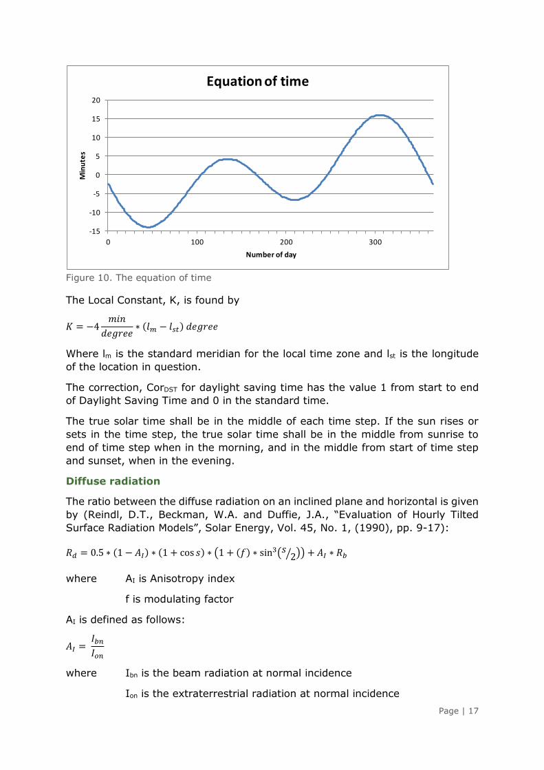
Tj varies from approximately -15 minutes to approximately + 17 minutes as can

be seen on Figure 10.

Page | 17

Figure 10. The equation of time

The Local Constant, K, is found by

𝐾 = −4𝑚𝑖𝑛

𝑑𝑒𝑔𝑟𝑒𝑒∗ (𝑙𝑚 − 𝑙𝑠𝑡) 𝑑𝑒𝑔𝑟𝑒𝑒

Where lm is the standard meridian for the local time zone and lst is the longitude

of the location in question.

The correction, CorDST for daylight saving time has the value 1 from start to end

of Daylight Saving Time and 0 in the standard time.

The true solar time shall be in the middle of each time step. If the sun rises or

sets in the time step, the true solar time shall be in the middle from sunrise to

end of time step when in the morning, and in the middle from start of time step

and sunset, when in the evening.

Diffuse radiation

The ratio between the diffuse radiation on an inclined plane and horizontal is given

by (Reindl, D.T., Beckman, W.A. and Duffie, J.A., “Evaluation of Hourly Tilted

Surface Radiation Models”, Solar Energy, Vol. 45, No. 1, (1990), pp. 9-17):

𝑅𝑑 = 0.5 ∗ (1 − 𝐴𝐼) ∗ (1 + cos 𝑠) ∗ (1 + (𝑓) ∗ sin3(𝑠2⁄ )) + 𝐴𝐼 ∗ 𝑅𝑏

where AI is Anisotropy index

f is modulating factor

AI is defined as follows:

𝐴𝐼 = 𝐼𝑏𝑛

𝐼𝑜𝑛

where Ibn is the beam radiation at normal incidence

Ion is the extraterrestrial radiation at normal incidence

-15

-10

-5

0

5

10

15

20

0 100 200 300

Min

ute

s

Number of day

Equation of time

Page | 18

f is defined as follows:

𝑓 = √𝐼𝑏

𝐼

The extraterrestrial radiation at normal incidence is set equal to the Solar

Constant.

The beam radiation at normal incidence is found by setting θ = 0.

Hereby the diffuse radiation on the inclined plane:

dddiff RII *

Reflected radiation

The contribution from radiation reflected from the ground is defined as follows:

*)cos1(*5,0 sRr

where is the reflection factor

depends on local conditions, a typical value is 0.2, equal to ground covered by

grass.

Hereby the reflected radiation becomes

rref RII *

Total radiation

The total radiation on the inclined surface is the sum of the beam, diffuse and

reflected radiation:

refdiffdirs IIII

Array shading

Without Array shading the calculated radiation on an inclined surface is valid for

single rows of surface. Often, large scale solar collector or photo voltaic systems

will be mounted on the ground in rows. The radiation will be reduced on the

subsequent rows.

An example here of can be seen on Figure 11.

Page | 19

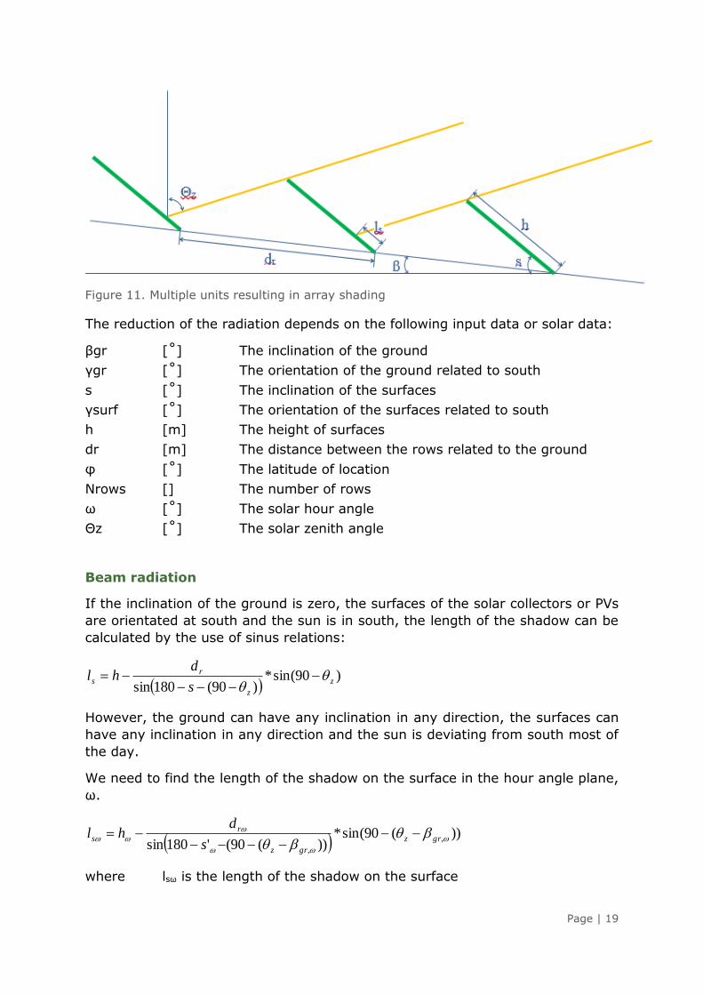
Figure 11. Multiple units resulting in array shading

The reduction of the radiation depends on the following input data or solar data:

βgr [˚] The inclination of the ground

γgr [˚] The orientation of the ground related to south

s [˚] The inclination of the surfaces

γsurf [˚] The orientation of the surfaces related to south

h [m] The height of surfaces

dr [m] The distance between the rows related to the ground

φ [˚] The latitude of location

Nrows [] The number of rows

ω [˚] The solar hour angle

Θz [˚] The solar zenith angle

Beam radiation

If the inclination of the ground is zero, the surfaces of the solar collectors or PVs

are orientated at south and the sun is in south, the length of the shadow can be

calculated by the use of sinus relations:

)90(sin*

)90(180sinz

z

rs

s

dhl

However, the ground can have any inclination in any direction, the surfaces can

have any inclination in any direction and the sun is deviating from south most of

the day.

We need to find the length of the shadow on the surface in the hour angle plane,

ω.

))(90(sin*

))(90('180sin,

,

grz

grz

rs

s

dhl

where lsω is the length of the shadow on the surface

Page | 20

hω is the height of the surface

drω is the distance between the rows

s’ω is the surface’s inclination related to the ground

βgr,ω is the inclination of the ground

All in the hour angle plane, ω.

The height of the surface in the hour angle, hω is found by the following cosine

relation:

ℎ𝜔 = √ℎ𝑔𝑟𝜔2 + (sin s ∗ h)2 − 2 ∗ ℎ𝑔𝑟𝜔 ∗ (sin s ∗ h) ∗ cos (90 − (𝛽𝑔𝑟,𝑠𝑢𝑟𝑓𝜔 − 𝛽𝑔𝑟𝜔))

where hgrω is the height of the surface, when projected down on the ground:

ℎ𝑔𝑟𝜔 = cos 𝑠 ∗ ℎ

cos(𝛽𝑔𝑟,𝑠𝑢𝑟𝑓𝜔 − 𝛽𝑔𝑟𝜔) ∗ cos 𝜔

The inclination of the ground in the hour angle, βgr,ω is found by:

𝛽𝑔𝑟,𝜔 = asin (sin 𝛽𝑔𝑟 ∗ cos(𝜔 − 𝛾𝑔𝑟))

The distance between the rows in the hour angle, drω is found by:

𝑑𝑟𝜔 = cos 𝛽𝑔𝑟,𝑠𝑢𝑟𝑓

cos(𝜔 − 𝛾𝑠𝑢𝑟𝑓) ∗ cos 𝛽𝑔𝑟,𝜔

∗ 𝑑𝑟

βgr,surf is the grounds inclination in the orientation of the surfaces:

𝛽𝑔𝑟,𝑠𝑢𝑟𝑓 = asin (sin 𝛽𝑔𝑟 ∗ cos(𝛾𝑠𝑢𝑟𝑓 − 𝛾𝑔𝑟))

The surface’s inclination in the hour angle related to the inclination of the ground:

𝑠′𝜔 = arcsin (sin(90 − 𝛽𝑔𝑟𝜔) ∗ sin 𝑠 ∗ ℎ

ℎ𝜔)

The part of the total surface area in shadow, Shfrac is calculated as follows

𝑆ℎ𝑓𝑟𝑎𝑐 = (𝑁𝑟𝑜𝑤𝑠 − 1) ∗ 𝑚𝑖𝑛 (

𝑙𝑠ℎ𝜔

, 1)

𝑁𝑟𝑜𝑤𝑠

where Nrows is the number of rows.

With correction for array shading the beam radiation becomes

𝐼𝑑𝑖𝑟 = 𝐼𝑏 ∗ 𝑅𝑏 ∗ (1 − 𝑆ℎ𝑓𝑟𝑎𝑐)

Diffuse radiation

The shadow impact on the diffuse radiation is visualized below.

Page | 21

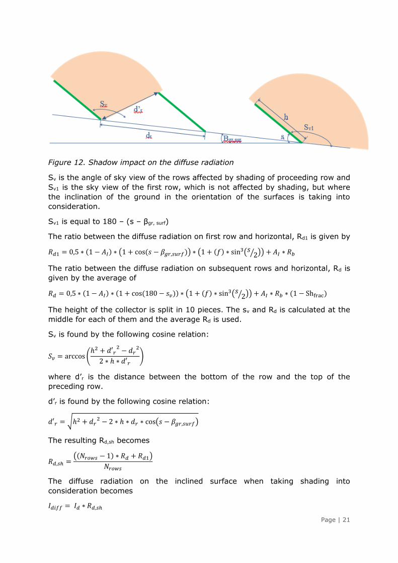
Figure 12. Shadow impact on the diffuse radiation

Sv is the angle of sky view of the rows affected by shading of proceeding row and

Sv1 is the sky view of the first row, which is not affected by shading, but where

the inclination of the ground in the orientation of the surfaces is taking into

consideration.

Sv1 is equal to 180 – (s – βgr, surf)

The ratio between the diffuse radiation on first row and horizontal, Rd1 is given by

𝑅𝑑1 = 0,5 ∗ (1 − 𝐴𝐼) ∗ (1 + cos(𝑠 − 𝛽𝑔𝑟,𝑠𝑢𝑟𝑓)) ∗ (1 + (𝑓) ∗ sin3(𝑠2⁄ )) + 𝐴𝐼 ∗ 𝑅𝑏

The ratio between the diffuse radiation on subsequent rows and horizontal, Rd is

given by the average of

𝑅𝑑 = 0,5 ∗ (1 − 𝐴𝐼) ∗ (1 + cos(180 − 𝑠𝑣)) ∗ (1 + (𝑓) ∗ sin3(𝑠2⁄ )) + 𝐴𝐼 ∗ 𝑅𝑏 ∗ (1 − Shfrac)

The height of the collector is split in 10 pieces. The sv and Rd is calculated at the

middle for each of them and the average Rd is used.

Sv is found by the following cosine relation:

𝑆𝑣 = arccos (ℎ2 + 𝑑′𝑟

2− 𝑑𝑟

2

2 ∗ ℎ ∗ 𝑑′𝑟)

where d’r is the distance between the bottom of the row and the top of the

preceding row.

d’r is found by the following cosine relation:

𝑑′𝑟 = √ℎ2 + 𝑑𝑟2 − 2 ∗ ℎ ∗ 𝑑𝑟 ∗ cos(𝑠 − 𝛽𝑔𝑟,𝑠𝑢𝑟𝑓)

The resulting Rd,sh becomes

𝑅𝑑,𝑠ℎ =((𝑁𝑟𝑜𝑤𝑠 − 1) ∗ 𝑅𝑑 + 𝑅𝑑1)

𝑁𝑟𝑜𝑤𝑠

The diffuse radiation on the inclined surface when taking shading into

consideration becomes

𝐼𝑑𝑖𝑓𝑓 = 𝐼𝑑 ∗ 𝑅𝑑,𝑠ℎ

Page | 22

Reflected radiation

The reflected radiation ratio when taking shading into consideration is divided into

the beam, Rr,b and diffuse, Rr, d radiation. Further, the ratio is different for the first,

Rr1 and the following rows, Rrn.

Beam and diffuse reflected radiation on the first rows are given as

𝑅𝑟1,𝑏 = 𝑅𝑟1,𝑑 = 0.5 ∗ (1 − cos(𝑠 − 𝛽𝑔𝑟,𝑠𝑢𝑟𝑓)) ∗ 0.2

The reflected radiation on the proceeding rows is calculated as ratio of the

reflected radiation on the first row, rp-1.

The beam reflected radiation on the proceeding rows depends on the length of the

beam on the ground, lsun. The length is zero if the surface is partly in shade,

meaning that no beam radiation reach the ground in front of the row.

If the length of the beam on the ground is equal to h, rp-1,b is set to 1. The length

is calculated as follows:

𝑙𝑠𝑢𝑛 = 𝑑𝑟𝜔 −ℎ𝜔

sin(90 − 𝜃′𝑧𝜔)∗ sin(180 − 𝑠′

𝜔 − (90 − 𝜃′𝑧𝜔))

And rp-1,b becomes

𝑟𝑝−1,𝑏 = 𝑙𝑠𝑢𝑛

ℎ

𝑅𝑟𝑛,𝑏 = 𝑅𝑟1,𝑏 ∗ 𝑟𝑝−1,𝑏

The reflected beam radiation, Rr,b becomes

𝑅𝑟,𝑏 =((𝑁𝑟𝑜𝑤𝑠 − 1) ∗ 𝑅𝑟𝑛,𝑏 + 𝑅𝑟1,𝑏)

𝑁𝑟𝑜𝑤𝑠

The reflected diffuse radiation on the proceeding rows as ratio of the reflected

diffuse radiation on the first row, rp-1,d has been defined as follows

𝑟𝑝−1,𝑑 = 𝑆𝑣

(180 − (𝑠 − 𝛽𝑔𝑟,𝑠𝑢𝑟𝑓))

The diffuse reflected radiation, Rrn,d becomes

𝑅𝑟𝑛,𝑑 = 𝑅𝑟1,𝑑 ∗ 𝑟𝑝−1,𝑑

The overall reflected diffuse radiation, Rr,d becomes

𝑅𝑟,𝑑 =((𝑁𝑟𝑜𝑤𝑠 − 1) ∗ 𝑅𝑟𝑛,𝑑 + 𝑅𝑟1,𝑑)

𝑁𝑟𝑜𝑤𝑠

The reflected radiation on the inclined surface when taking shading into

consideration becomes

𝐼𝑟𝑒𝑓 = 𝐼𝑏 ∗ 𝑅𝑟,𝑏 + 𝐼𝑑 ∗ 𝑅𝑟,𝑑

Page | 23

Solar Collector

The formula for a solar collector is as follows (without Incidence angle modifier):

2

21 **** amamos ttattanIAY

where

Y: heat production, [W].

A: Solar collector area [m2]

Is: Solar radiation on solar collector, [W/m2]

tm: The collectors average temperature, [oC], that is an average between

the temperature of the cold water entering the collector and the hot

water leaving the collector

ta: The ambient temperature, [oC]. For the best results the ambient

temperatures should be hourly.

The efficiency of the solar collector is defined by three parameters:

no: Intercept (maximum) of the collector efficiency, [-]

a1: The first-order coefficient in collector efficiency equation, [W/(m2 C)]

a2: The second-order coefficient in collector efficiency equation, [W/(m2

C2)]

These 3 parameters are available for collectors tested according to ASHRAE

standards and rated by SRCC (ASHRAE, 2003; SRCC,1995), as well as for

collectors tested according to the recent European Standards on solar collectors

(CEN, 2001). Many examples of collector parameters can be found on the internet

(e.g. SPF, 2004).

Note: It is important to make sure that collector area entered as a parameter

match the area used when determining the values of no, a1 and a2. Typically,

efficiency curves are provided for gross area in the US and aperture area in

Europe.

Furthermore, the model includes Incidence Angle Modifier, IAM or K. The sun is

not always located perpendicular to the collector plane; the incidence angle

generally changes both during the course of a day and throughout the year. The

transmittance of the cover glazing for the collector changes with the incidence

angle.

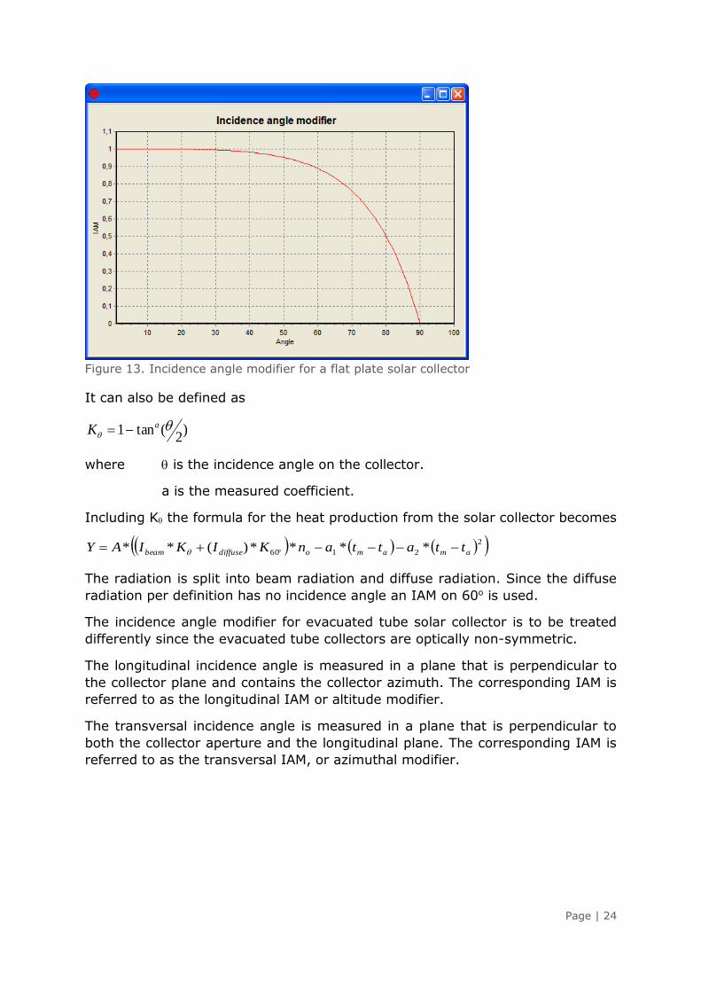
Typically, the Incidence angle modifier for a flat plate solar collector looks as the

one shown on Figure 13.

Page | 24

Figure 13. Incidence angle modifier for a flat plate solar collector

It can also be defined as

)2

(tan1

aK

where is the incidence angle on the collector.

a is the measured coefficient.

Including K the formula for the heat production from the solar collector becomes

2

2160 ****)(** amamodiffusebeam ttattanKIKIAY

The radiation is split into beam radiation and diffuse radiation. Since the diffuse

radiation per definition has no incidence angle an IAM on 60o is used.

The incidence angle modifier for evacuated tube solar collector is to be treated

differently since the evacuated tube collectors are optically non-symmetric.

The longitudinal incidence angle is measured in a plane that is perpendicular to

the collector plane and contains the collector azimuth. The corresponding IAM is

referred to as the longitudinal IAM or altitude modifier.

The transversal incidence angle is measured in a plane that is perpendicular to

both the collector aperture and the longitudinal plane. The corresponding IAM is

referred to as the transversal IAM, or azimuthal modifier.

Page | 25

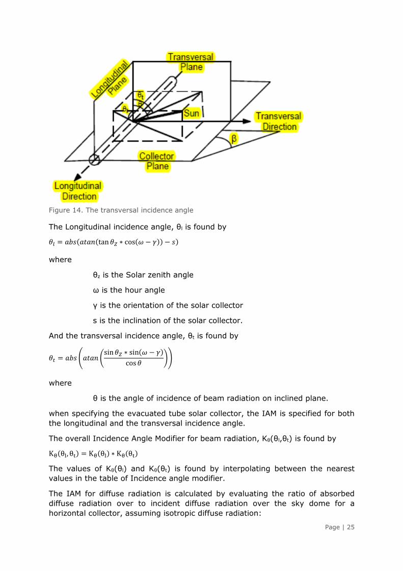
Figure 14. The transversal incidence angle

The Longitudinal incidence angle, θl is found by

𝜃𝑙 = 𝑎𝑏𝑠(𝑎𝑡𝑎𝑛(tan 𝜃𝑍 ∗ cos(𝜔 − 𝛾)) − 𝑠)

where

θz is the Solar zenith angle

ω is the hour angle

γ is the orientation of the solar collector

s is the inclination of the solar collector.

And the transversal incidence angle, θt is found by

𝜃𝑡 = 𝑎𝑏𝑠 (𝑎𝑡𝑎𝑛 (sin 𝜃𝑍 ∗ sin(𝜔 − 𝛾)

cos 𝜃))

where

θ is the angle of incidence of beam radiation on inclined plane.

when specifying the evacuated tube solar collector, the IAM is specified for both

the longitudinal and the transversal incidence angle.

The overall Incidence Angle Modifier for beam radiation, Kθ(θl,θt) is found by

Kθ(θl, θt) = Kθ(θl) ∗ Kθ(θt)

The values of Kθ(θl) and Kθ(θt) is found by interpolating between the nearest

values in the table of Incidence angle modifier.

The IAM for diffuse radiation is calculated by evaluating the ratio of absorbed

diffuse radiation over to incident diffuse radiation over the sky dome for a

horizontal collector, assuming isotropic diffuse radiation:

Page | 26

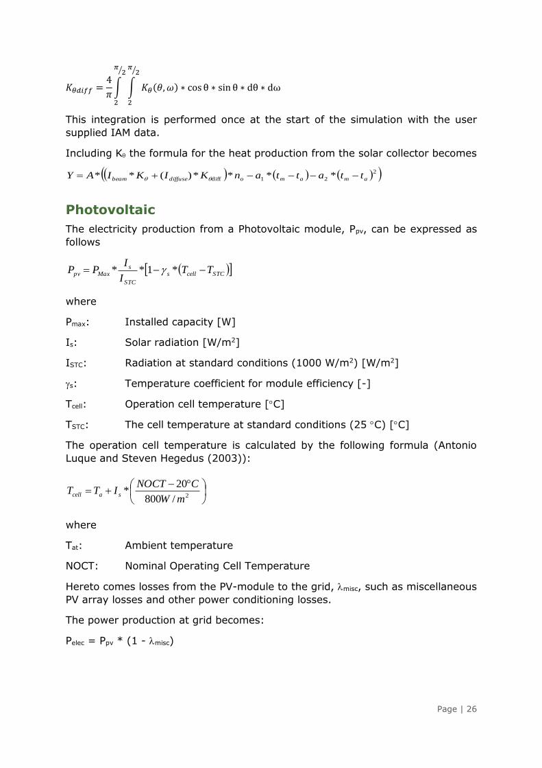
𝐾𝜃𝑑𝑖𝑓𝑓 =4

𝜋∫ ∫ 𝐾𝜃(𝜃, 𝜔) ∗ cos θ ∗ sin θ ∗ dθ ∗ dω

𝜋2⁄

2

𝜋2⁄

2

This integration is performed once at the start of the simulation with the user

supplied IAM data.

Including K the formula for the heat production from the solar collector becomes

2

21diff ****)(** amamodiffusebeam ttattanKIKIAY

Photovoltaic

The electricity production from a Photovoltaic module, Ppv, can be expressed as

follows

STCcells

STC

sMaxpv TT

I

IPP *1**

where

Pmax: Installed capacity [W]

Is: Solar radiation [W/m2]

ISTC: Radiation at standard conditions (1000 W/m2) [W/m2]

s: Temperature coefficient for module efficiency [-]

Tcell: Operation cell temperature [C]

TSTC: The cell temperature at standard conditions (25 C) [C]

The operation cell temperature is calculated by the following formula (Antonio

Luque and Steven Hegedus (2003)):

2/800

20*

mW

CNOCTITT sacell

where

Tat: Ambient temperature

NOCT: Nominal Operating Cell Temperature

Hereto comes losses from the PV-module to the grid, misc, such as miscellaneous

PV array losses and other power conditioning losses.

The power production at grid becomes:

Pelec = Ppv * (1 - misc)

Page | 27

Please notice, that you can find more information on how to use energyPRO in the

How to Guides, User’s Guide and tutorials on EMD’s website:

http://www.emd.dk/energypro/

Niels Jernes vej 10 · 9220 Aalborg Ø · Denmark

tel.: +45 9635 4444 · e-mail: emd@emd.dk · www.emd.dk