


Languages
Pages
Legal


Snowfall-Rate Retrieval for K- andW-Band Radar Measurements Designed in Hyytiälä, Finland,and Tested at Ny-Ålesund, Svalbard, Norway
SYBILLE Y. SCHOGER,a DMITRI MOISSEEV,b,c ANNAKAISA VON LERBER,c SUSANNE CREWELL,a AND
KERSTIN EBELLa
a Institute for Geophysics and Meteorology, University of Cologne, Cologne, Germanyb Institute for Atmospheric and Earth System Research/Physics, Faculty of Science, University of Helsinki, Finland
c Finnish Meteorological Institute, Helsinki, Finland
(Manuscript received 22 April 2020, in final form 4 December 2020)
ABSTRACT: Two power-law relations linking equivalent radar reflectivity factor Ze and snowfall rate S are derived for a
K-bandMicroRainRadar (MRR) and for aW-band cloud radar. For the development of theseZe–S relationships, a dataset
of calculated and measured variables is used. Surface-based video-disdrometer measurements were collected during
snowfall events over five winters at the high-latitude site in Hyytiälä, Finland. The data from 2014 to 2018 include particle
size distributions (PSD) and their fall velocities, from which snowflake masses were derived. The K- and W-band Ze values
are computed using these surface-based observations and snowflake scattering properties as provided by T-matrix and
single-particle scattering tables, respectively. The uncertainty analysis shows that the K-band snowfall-rate estimation is
significantly improved by including the intercept parameter N0 of the PSD calculated from concurrent disdrometer mea-
surements. If N0 is used to adjust the prefactor of the Ze–S relationship, the RMSE of the snowfall-rate estimate can be
reduced from 0.37 to around 0.11mmh21. ForW-band radar, aZe–S relationship with constant parameters for all available
snow events shows a similar uncertainty when compared with the method that includes the PSD intercept parameter. To
demonstrate the performance of the proposed Ze–S relationships, they are applied to measurements of the MRR and the
W-band microwave radar for Arctic clouds at the Arctic research base operated by the German Alfred Wegener Institute
Helmholtz Centre for Polar and Marine Research (AWI) and the French Polar Institute Paul Emile Victor (IPEV)
(AWIPEV) in Ny-Ålesund, Svalbard, Norway. The resulting snowfall-rate estimates show good agreement with in situ
snowfall observations while other Ze–S relationships from literature reveal larger differences.
KEYWORDS: Arctic; Precipitation; Snow; Snowfall; Radars/Radar observations; Remote sensing
1. Introduction
Solid precipitation and its deposition as snow are of great
importance for Earth’s energy budget and its hydrological
cycle. Especially in the Arctic and already at latitudes higher
than 608N, snowfall is the predominant precipitation type
(Levizzani et al. 2011). We know today that temperatures are
rising about 2 times faster in the Arctic than anywhere else on
Earth due to global warming (IPCC 2007; Serreze and Barry
2011), known as Arctic amplification. This has a great effect on
the hydrological cycle and the transformation of precipitation
from mainly solid to more liquid precipitation (López-Moreno
et al. 2016; Maturilli et al. 2013). Thus, to observe the effects of
climate change better, there is an urgent need to monitor long-
term snowfall at the northern high latitudes. However, espe-
cially in the Arctic, a ground-based observational precipitation
network is scarce and the environmental conditions such as
weather and orography are harsh for instrumentation (Førlandet al. 2011). Additionally, the measurement of snow particles
and the identification of the true amount of snow at the ground
is a challenging task due to the complex and strongly variable
microphysical properties of snow and ice crystals. For classical
precipitation gauges, the liquid equivalent amount of snow is a
direct measure; however, it is prone to large uncertainties es-
pecially in windy conditions (Rasmussen et al. 2012) and still
only a point information of precipitation. Radar provides more
information on the spatial distribution of precipitation, but
snowfall rate (S; mmh21) is an indirect measure and has to be
obtained from the equivalent radar reflectivity (further, often
just reflectivity) (Ze; mm6m23 or dBZ). The relationship be-
tween Ze and S is traditionally retrieved via the power law
Ze 5 azs Sbzs . The prefactor azs has the unit of mm62bzs hbzs m23
(in later sections omitted for better readability), and the ex-
ponent bzs is unitless.
More than 60 years of research have yielded many publica-
tions on different Ze–S relationship parameters (e.g., Langille
and Thain 1951; Carlson and Marshall 1972; Fujiyoshi et al.
1990; Rasmussen et al. 2003; Huang et al. 2010; von Lerber
et al. 2017), because for each snow event, each measurement
location, and each radar wavelength used the parameters of the
Ze–S relationship differ significantly. Radar snowfall-rate re-
search began by analyzing reflectivity measurements from
weather radars that measure at centimeter wavelengths. Many
of the Ze–S relationships for weather radars have been de-
termined with the prefactor azs ranging, for example, be-
tween values of 160 and 3300 and bzs between 1.5 and 2.2,
which are summarized by Rasmussen et al. (2003). In the
1980s, Lhermitte (1987, 1988) has pioneered the investigation
Denotes content that is immediately available upon publica-
tion as open access.
Corresponding author: Kerstin Ebell, [email protected]
MARCH 2021 S CHOGER ET AL . 273
DOI: 10.1175/JAMC-D-20-0095.1
� 2021 American Meteorological Society. For information regarding reuse of this content and general copyright information, consult the AMS CopyrightPolicy (www.ametsoc.org/PUBSReuseLicenses).
Unauthenticated | Downloaded 12/17/21 02:01 AM UTC

of nonprecipitating clouds from millimeter wavelength radars.
Kollias et al. (2007) argued that these radars can also be used
for precipitation even though attenuation is significant. For
solid precipitation, especially dry snowfall, however, attenua-
tion for W-band radar is small relative to rainfall (Matrosov
et al. 2008). The prefactor value range for theZe–S relationship
reduces by an order of magnitude when using millimeter
wavelength radars instead of weather radars. For example, the
range is only between 2.19 and 313.29 for the prefactor and 0.8
and 1.85 for the exponent (Matrosov 2007; Kulie and Bennartz
2009; Souverijns et al. 2017, hereinafter S17).
In 2006, the satellite CloudSat (Stephens et al. 2002) was
launched with the 94-GHz (3.19 mm wavelength) Cloud
Profiling Radar (CPR) that provides operational near-global
active snowfall measurements, to this day. Especially over the
polar regions, this measure is unique and important. However,
the expected lifetime is already exceeded (Stephens et al. 2018)
and the so-called blind zone in the lowest 1200m leads both to
misses and false alarms in surface snowfall events with an av-
erage precipitation underestimation of around 10% (Maahn
et al. 2014).
The motivation and aim of this study is to operationally re-
trieve snowfall rates from a ground-based radar at high-
latitude observational sites. The robust and low-cost Micro
Rain Radar (MRR) is frequently used at different sites around
the globe, however, just recently installed for operational use
in the Arctic at the research base operated by the German
Alfred Wegener Institute Helmholtz Centre for Polar and
Marine Research (AWI) and the French Polar Institute Paul
Emile Victor (IPEV) (AWIPEV) at Ny-Ålesund, Svalbard,
Norway. With the improved processing method for snow ob-
servations proposed by Maahn and Kollias (2012), the MRR
has emerged as a promising device for autonomous snowfall
monitoring and is used, for example, already in Antarctica
since 2010 (S17).
To retrieve parameters for the Ze–S relationship, two dif-
ferent approaches exist. One approach connects measured Ze
to ground-based in situ observations. The latter are used from
either gauges (Fujiyoshi et al. 1990) or disdrometers (Huang
et al. 2010) to obtain constant parameters over a longer time
period or for a set of snow events. Another approach is an
analytical retrieval of the snowfall rate considering the particle
size distribution (PSD) of the snow particles, which can be
measured or taken from literature (Heymsfield et al. 2016; von
Lerber et al. 2017).
Within this paper, we use both approaches to retrieve Ze–S
relationships for two different radar frequencies: for theMRR,
which measures at 24GHz in the K band, and for a W-band
radar, that measures at the same frequency as the CloudSat
CPR. To calculate snowfall rates from the MRR, Ze–S rela-
tionships for 35-GHz radars have been used in the past (e.g.,
Kneifel et al. 2011; Maahn et al. 2014). Recently, a Ze–S
relationship for MRR has been developed but only for
Antarctica (S17).
We, on the contrary, develop a new relationship particularly
suited for a 24-GHz radar. Additionally, we use a new ap-
proach to keep the prefactor azs variable in time by adding
information from concurrent surface observations. We make
use of the instantaneous PSD from a disdrometer as
Rasmussen et al. (2003) have shown that azs depends strongly
on the intercept parameter N0 of the PSD in the Rayleigh
scattering regime. With this approach, the Ze–S relationship
takes the local variability of the PSD into account. Thus, the
method is less restricted to the location for which it was orig-
inally developed. Using this new method compared to a
method with a constant azs, it is expected to improve the re-
sulting snowfall rate. Furthermore, we calculate the snowfall
rate also with Ze from a W-band radar to have an indepen-
dently derived snowfall rate to which the results from the
K-band radar can be compared to. The comparison of the re-
sulting snowfall accumulation to an observational in situ ref-
erence completes the analysis.
For the derivation of the Ze–S relationship parameters azsand bzs, information on microphysical properties of snow
particles is required (S17) but not always available or suffi-
ciently well known. These required properties are the terminal
fall velocity, PSD,mass, and the backscatter cross section of the
ice particles, where the latter is different for each radar frequency.
At the high-latitude measurement site in Hyytiälä, Finland, thevideo-disdrometer Precipitation Imaging Package (PIP) directly
measures fall velocity andPSDof snowevents fromwhichmass of
the snow particles is calculated with hydrodynamic theory (von
Lerber et al. 2017). In this studywe use snow eventmeasurements
from five winters between 2014 and 2018.
In section 2, we give an overview on the measurement sites
and data sources. In section 3, we introduce the basics of the
radar-based snowfall-rate retrieval. Section 4 is divided into
two parts. First, the Ze–S retrieval development is explained in
detail together with an uncertainty analysis based on data from
Hyytiälä. Second, because there are no reliable MRR obser-
vations available in Hyytiälä during the same time when a
cloud radar has beenmeasuring, we test the performance of the
new snowfall-rate retrieval methods with measurements from
AWIPEV atNy-Ålesund. At this site, the retrieved parameters
are applied to measured Ze values from an MRR and the
W-bandMicrowaveRadar forArctic Clouds (MiRAC-A). The
performance of the newly developed relationships is then
evaluated for three case studies. A summary of the results and
conclusions can be found in section 5.
2. Measurement setup
a. Measurement site Hyytiälä
The University of Helsinki operates a Forestry Field Station
in southern Finland, in Hyytiälä (61.84398N, 24.28758E; 150mabove mean sea level), 220 km northwest of Helsinki (Hari and
Kulmala 2005). Meteorological instrumentation, including the
PIP, is operated in the middle of a clearing since 2014. The PIP
is a video disdrometer from the National Aeronautics and
Space Administration deployed to Hyytiälä as part of the
Global Precipitation Measurement mission (GPM) ground
validation program. It is the successor of the Snow Video
Imager (SVI) (Newman et al. 2009) with an improved camera
and software (Tiira et al. 2016). The principle of this instrument
is taking highly resolved images with a video camera that has a
frame rate as high as 380 frames per second, which is directed
274 JOURNAL OF APPL IED METEOROLOGY AND CL IMATOLOGY VOLUME 60
Unauthenticated | Downloaded 12/17/21 02:01 AM UTC

toward a 2-m-distant halogen lamp acting as a background il-
lumination (Tiira et al. 2016). The measurement volume is
determined by the field of view (48mm 3 64mm) and the
depth of field (defined by the particles in focus). Particles
falling through the volume between light and camera are
recorded and a 2D-grayscaled video image is saved. The disk-
equivalent diameter Ddeq, that is, the same area of a circular
disk as the mapped shadowed area, is then defined from the
particle image with a resolution of 0.1mm 3 0.1mm (Newman
et al. 2009). The diameterDdeq ranges from 0.1 to 26mm and is
divided into 130 bins, whereas the last bin includes every particle
with diameter larger than 26mm (von Lerber et al. 2018). The
error of the provided particle size from the predecessor of PIP
is estimated to be 18% (error in Ddeq) (Newman et al. 2009).
Due to the observation of consecutive frames at high rate,
the fall velocity of a single particle as a function of Ddeq
(hereafterD) is recorded. Since the Hyytiälämeasurement site
is located in a forest-sheltered clearing, the surrounding wind
conditions are typically modest or low (mean wind in snowfall
cases during 2014–18 is 1.5m s21 and the vertical wind com-
ponent was much smaller than the fall velocity) as can be ob-
served with observations from a collocated 3D anemometer.
Therefore, it is assumed that the effect of vertical air velocity is
small compared to the particle fall velocity, and in the mass
retrieval, fall velocity is assumed to be close to the snowflake
terminal velocity. This naturally induces uncertainty in the
derived masses (Zawadzki et al. 2010). Additionally, as a
function of D, the PSD is determined for every minute.
b. Measurements at AWIPEV, Ny-Ålesund
The French–German Arctic research base AWIPEV is lo-
cated on the Norwegian archipelago Svalbard, in the village of
Ny-Ålesund (78.92308N, 11.92108E; 11m above mean sea
level). The village is situated at the Kongsfjord and close to
mountains that are located parallel to the Fjord from northwest
to southeast.
Since 2016, the University of Cologne (UoC) is part of the
Transregional Collaborative Research Centre (TR 172) on
Arctic Amplification: Climate Relevant Atmospheric and
Surface Processes, and Feedback Mechanisms (AC)3 (Wendisch
et al. 2017; Wendisch et al. 2018). Within this project, the UoC
operates a cloud radar in Ny-Ålesund with continuous mea-
surements from June 2016 to October 2018 and from June 2019
onward. Since April 2017, continuous measurements from an
MRR and the laser disdrometer Particle Size Velocity
(PARSIVEL) of UoC are available as well. These instruments
are located on the roof of the AWIPEV observatory.
Additionally, used as auxiliary variables in the later case
study, measurements from a 10-m tower that include wind and
temperature at 2- and 10-m height are available from the
Baseline Surface Radiation Network (BSRN) site, operated by
AWI (Maturilli 2018). A detailed description about the me-
teorological sensors installed on the tower and the BSRN site
in general can be found in Maturilli et al. (2013).
AWI’s humidity and temperature profiler (HATPRO), a
microwave radiometer, provides information on vertically in-
tegrated liquid water in the atmospheric column, that is, the
liquid water path (LWP; Nomokonova et al. 2019a), which is
used in this study to detect precipitation and indicate riming.
Details on the LWP retrieval can be found in Nomokonova
et al. (2019a). The temporal resolution of the LWP is 1–2 s. The
LWP accuracy is within 20–25 gm22 (Rose et al. 2005).
1) LASER DISDROMETER: PARSIVEL
PARSIVEL is an optical laser-disdrometer produced by the
manufacturer OTT. A flat laser sheet is transmitted at 650 nm
with an area of 27mm 3 180mm and a height of 1mm
(Battaglia et al. 2010). A voltage decrease occurs when the
laser sheet is blocked by particles falling between transmitter
and receiver. The fall velocity is measured via the time delay of
the particle intercepting the laser beam. Particle size is pro-
portional to the amplitude of the voltage decrease.
Within PARSIVEL’s retrieval rationale, measured particles
are assumed to be raindrop-like, thus, small particles (diameter
smaller than 1mm) are assumed to be spherical. In the middle
range (1–5mm) particles are assumed to be horizontally ori-
ented oblate spheroids with axial ratio linearly varying from 1
to 0.7 and larger particles (larger than 5mm) have constant
axial ratio of 0.7 (Battaglia et al. 2010). The provided output
diameter for raindrops can therefore be interpreted as a vol-
ume equivalent diameter; however, for irregularly shaped
snowflakes, the diameter definition is more arbitrary. Battaglia
et al. (2010) have investigated PARSIVEL’s ability to measure
falling snow in more detail. They found an underestimation of
fall velocity for small snow particles and an overestimation for
large particles with up to 30%–40% uncertainty. The uncer-
tainty in particle size and fall velocity propagates into the PSD
retrieval of the instrument. In this study, we use the measured
PSD to fit an exponential function and to retrieve the intercept
parameter N0. A comparison between the fitted exponential
PSD from PIP and a PARSIVEL measuring in Hyytiälä (not
shown) revealed a small difference (mean difference in respect
to the range of values is 1.7%) inN0, from which we concluded
that the retrieved N0 with PARSIVEL can be applied to the
later defined Ze–S relation for MRR in section 4.
2) MICRO RAIN RADAR
The MRR is a vertically pointing frequency modulated
continuous wave (FM-CW) Doppler radar manufactured by
METEK GmbH (Klugmann et al. 1996). It operates at a fre-
quency of f 5 24GHz (K band; wavelength l 5 12.38mm).
Relative to (pulsed) radars in the same frequency range, the
MRR has a low power consumption of 25W. If the installed
dish heater is turned on, a consumption of 500W is added. The
heating system prevents snow accumulation on the parabolic
offset dish antenna, which has an effective aperture diameter of
0.5m. The beamwidth of the signal is 1.58. All output variables
are internally averaged over 10-s time steps to generate a 1-min
data resolution.
The MRR was originally built to measure liquid precipita-
tion and was not well suited for solid precipitation. Maahn and
Kollias (2012) developed an Improved MRR Processing Tool
(IMProToo) for better snow observations through dealiasing
the Doppler spectra and removing noisy signals. The lowest
detectable value thus decreased from 25 dBZ for Metek’s
standard analyzing method to 214 dBZ for the new proposed
MARCH 2021 S CHOGER ET AL . 275
Unauthenticated | Downloaded 12/17/21 02:01 AM UTC
method byMaahn and Kollias (2012). At Ny-Ålesund, the first
MRRbin is at a height of 30m.The vertical resolution of the radar
bins is set to 30m resulting in a maximum height range of 930m.
We are interested in snowfall at the ground, but the lowest radar
bins usually suffer from noisy signals. Additionally, the snowfall
rate calculated from MRR is compared to the snowfall rate
from theW-band radar, whose lowest radar bin is at a height of
about 100m (see next section). For the MRR, we thus
calculated a vertically averaged Ze from the three range bins
between 120 and 180m for each time step.
3) MICROWAVE RADAR/RADIOMETER FOR ARCTIC
CLOUDS
The active component of MiRAC is a W-band radar
(MiRAC-A), operating at f 5 94GHz (l 5 3.19mm) and
manufactured by Radiometer Physics GmbH. The separation
into one transmitting and one receiving antenna (beamwidth of
0.488) allows the continuous wave transmission and the re-
ceiving antenna is protected from saturation (Küchler et al.
2017). MiRAC-A has a very low transmitter power consump-
tion of 1.5W but a strong blower that ensures a precipitation-
free antenna surface. The uncertainty of Ze is on the order of
0.5 dBZ, and the lowest detectable signal is in the range of265
to 250 dBZ at the distance of 100–600m depending on chirp
settings and atmospheric state (Mech et al. 2019). The available
height range starts at about 100m and can reach up to 12 km
with a vertical resolution of maximum 3.2m. Similar to MRR,
we averaged the cloud radar Ze over the height range between
120 and 180m above ground. The internal time sampling is
at a rate of 2.4 s; however, to have a better comparison to the
MRR measurements, we average the values over 1min.
4) PRECIPITATION GAUGE: PLUVIO
The Pluvio2 L 400 (herein, Pluvio) is an automated weighing
gauge with an orifice of 400 cm2 and is manufactured by OTT.
The gauge is suitable for observing both liquid and solid pre-
cipitation. The latter is always given as the amount equivalent
to liquid water and the phase distinction need to be obtained
via temperature measurements. In this study, we use the non-
real time accumulated precipitation in mmh21 that has an
absolute (relative) accuracy of 60.1mm (61%) (OTT 2016).
In general, gauges are very prone to the underestimation of
solid precipitation due to high wind, or overestimation due to
blowing snow. Therefore, different wind shieldings have been
designed, used, and tested in the last decades to limit the un-
certainty of gauge measurements (Rasmussen et al. 2012). The
Pluvio in Ny-Ålesund is surrounded by a single Alter wind
shield. Rasmussen et al. (2014) compared a single Alter wind
shield to a Double-Fence Intercomparison Reference gauge in
dry snowfall and found that the undercatchment of snow is
approximately less than 30% with the single Alter wind shield
at a wind speed smaller than 5m s21 increasing to 60% with
higher wind speeds of 9m s21 or more.
3. Radar-based snowfall-rate retrieval
Because of the complex microphysics of snow, the correct
estimation of snowfall from radar measurements remains
especially challenging as the parameter values for the Ze–S
relationship are numerous and typically event specific.
a. Snowfall rate
The snowfall rate in the liquid equivalent units of millime-
ters per hour can be calculated from the density of liquid water
rw, the mass–size relationship m(D), the fall velocity–size re-
lationship y(D), all in SI units, and the PSDN(D) (mm21m23):
S53600
rw
ðDmax
Dmin
m(D)y(D)N(D) dD . (1)
The Dmin and Dmax are the minimum and maximum observed
particle size of PIP (Ddeq), respectively, with both in units of
millimeters.
For this study, a dataset consisting of the variables y(D, t),
N(D, t), and m(D, t) were used. These variables have been
derived from the PIPmeasurements with whichwe calculated a
time-dependent snowfall rate, because all measurements are
averaged over a 5-min time interval where temperatures were
below 08C. In total, 4947 of these time intervals are available
from five winters between 31 January 2014 and 2 April 2018.
The first two years of this dataset (Moisseev 2020) are de-
scribed in Tiira et al. (2016) and von Lerber et al. (2017) and
utilized in, for example, Moisseev et al. (2017), Falconi et al.
(2018), Li et al. (2018), Mason et al. (2018), Leinonen et al.
(2018), Mason et al. (2019), Tyynelä and von Lerber (2019),
and Chase et al. (2020). The dataset used in this study uses
measurements of additional three years but is based on the
cited dataset.
The fall velocity of snow particles and PSD are a direct
output of PIP. To account for a continuous size distribution,
the measured 5-min mean PSD is approximated with the
exponential function: N(D) 5 N0 exp(2LD). To derive the
exponential PSD, the intercept parameter N0(t) and the slope
L(t) are calculated with the method of moments (e.g.,
Moisseev and Chandrasekar 2007; Ulbrich and Atlas 1998)
from the PSD measured by PIP. The applied mass retrieval is
from von Lerber et al. (2017), where the parameterization of
Mitchell and Heymsfield (2005) for the hydrodynamic theory
has been utilized and showed to describe the climatological
snow conditions in Finland well. In hydrodynamic theory, the
gravity and atmospheric drag influencing the falling particle
are set equal, and therefore the mass of a snowflake can be
estimated from observations of fall velocity, particle dimen-
sions, and area characteristics.
b. Reflectivity
The equivalent radar reflectivity factor can be computed as
Ze5
l4
p5jKj2ðDmax
Dmin
sb(D)N(D) dD , (2)
where Ze is given in linear units. The wavelength l is in milli-
meters; the dielectric factor jKj2 is unitless; the backscatter
cross section sb(D) is in millimeters squared, and Dmin, Dmax,
and N(D) have the same units as in Eq. (1). In this study, we
calculate Ze for two different wavelengths as well as for 5-min
time intervals. Thus, we use the time-dependent exponential
276 JOURNAL OF APPL IED METEOROLOGY AND CL IMATOLOGY VOLUME 60
Unauthenticated | Downloaded 12/17/21 02:01 AM UTC

N(D, t) in Eq. (2), which has been fitted to the observations as
described in the previous section. For the dielectric factor,
which depends onwavelength and temperature, we used jKj250.92 for K band and ;0.76 for W band. Also, wavelength-
dependent sb(D) values were computed using different ap-
proaches that are explained in the following.
For the MRR frequency (K band), that is, 24GHz, the soft-
spheroid particle model in combination with effective medium
approximation (Sihvola 1999) and T-matrix method (TMM)
can be applied (Tyynelä et al. 2011; Falconi et al. 2018).
Although it is shown (e.g., in Schrom and Kumjian 2018) that
for single crystals the dual-polarization scattering properties
cannot be adequately computed with soft-spheroid approxi-
mation, here, we apply the approximation for snow particle
mixtures, and on average, the forward simulated Ze is rea-
sonably well described compared to observations at K band
(Falconi et al. 2018). At higher frequencies, for example,
W band, this particle model starts to fail (Leinonen et al. 2012;
Kneifel et al. 2015). To compute the K-band Ze, the soft-
spheroid particlemodel with an aspect ratio of 0.6, which works
both for rimed and unrimed snowflakes (Li et al. 2018), was
used. Given the particle mass, maximumdimension, and aspect
ratio, the snowflake refractive index is computed using the
Bruggeman approximation (Bruggeman 1935). The backscat-
tering cross section of snowflakes are then computed using
TMM (Mishchenko and Travis 1994; Leinonen 2014, 2018).
To calculate sb for theW band, the single-particle scattering
databases of Leinonen and Moisseev (2015), Leinonen and
Szyrmer (2015), and Tyynelä and von Lerber (2019) were used.All databases are different and represent particles with dif-
ferent properties. The snowflakes were modeled mimicking
physical processes responsible for ice particle formation, vapor
deposition, aggregation (Leinonen and Moisseev 2015), and,
additionally, riming (Leinonen and Szyrmer 2015), or as fractal
particles (Tyynelä and von Lerber 2019). The scattering
properties of these complex particles are computed using the
discrete dipole approximation (DDA) (Yurkin and Hoekstra
2011). To determine a backscattering cross section for a given
snowflake we have used linear interpolation in the log–log
space, where sb(D) is a function of the maximum dimension
and particle mass. For this, all the databases were combined
into one.
4. Results
a. Snowfall-rate retrieval development
For the development of the snowfall-rate retrieval, we
solved the Ze–S relationship for S. and used the following
equation for further calculations:
S5
1
azs
Ze
!1/bzs
. (3)
Two methods are developed to retrieve azs and bzs and are
presented in the following subsections. An overview scheme of
all variables (measured, derived, and simulated) and how they
are used to calculate Ze and S is shown in Fig. 1.
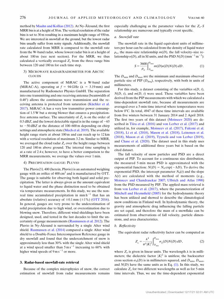
1) AVERAGE ZE–S RELATIONSHIP
For the so-called average Ze–S relationship the calculated
reflectivity [Eq. (2)] is plotted against the calculated snowfall
rate [Eq. (1)] on logarithmic scales for all available 4947 five-
minute time steps for both the K-band and the W-band radars.
From the resulting scatterplot (Fig. 2) the exponent and pre-
factor can be derived with a total least squares fit (TLS or or-
thogonal distance regression) (Boggs and Rogers 1990; Boggs
et al. 1992), which accounts for the uncertainty in both S and
Ze. For K band, the parameters azs 5 77.61 and bzs 5 1.22 are
obtained. For W band, we get azs 5 18.18 and bzs 5 0.98. By
constraining the exponent value bzs to be constant, the 0.05 and
0.95 quantile for the prefactor can be derived from the TLS fit.
The value range of 30.15 # azs # 205.83 for K band shows the
wide variation of the prefactor values. For W band, the value
range is lower with 11.22 # azs # 28.36. Especially in the
K-band frequency, for one specific Ze value, a variety of dif-
ferent S values in the order of a magnitude can be retrieved
(e.g., for Ze 5 1021mm6m23 the range in S is from 10 to
1022mmh21). By definition, the prefactor variation inW band
is smaller because of a smaller Ze range with a maximum Ze of
102mm6m23 as compared with 103mm6m23 for K band (see
Fig. 2). For further reference, this method is called AVE_K
and AVE_W for the average relationship for K and W band,
respectively.
2) ANALYTICAL ZE–S RELATIONSHIP
Following von Lerber et al. (2017), our so-called analytical
Ze–S relationship considers the time-dependency of all pa-
rameters and provides an instantaneous Ze–S relationship for
each time step. For better readability, the time dependency of
each variable is omitted in the following equations.
When assuming power laws for the mass– and fall velocity–
dimensional relationships, the exponential PSD function, and
by integrating over an infinite diameter size on which the
complete Gamma function can be applied, Eq. (1) can be re-
written into more detailed components:
S51
rw
ð‘0
amDbma
yDbyN
0exp(2LD)dD
51
rw
amayN
0L2(bm1by11)G(b
m1 b
y1 1)
5N0FSG(b
m1b
y1 1), (4)
where FS comprises the remaining variables.
Doing the same for the reflectivity, Eq. (2) can be written as
Ze5
l4
p5jKj2ð‘0
asDbsN
0exp(2LD) dD
5l4
p5jKj2 asN0L2(bs11)G(b
s1 1)
5N0FZeG(b
s1 1). (5)
By inserting Eqs. (4) and (5) into the Ze–S relationship, the
analytical solution for the two parameters in dependency of
time is obtained
MARCH 2021 S CHOGER ET AL . 277
Unauthenticated | Downloaded 12/17/21 02:01 AM UTC

Ze5N
0FZe(N
0FS)
�2
�bs11
bm1b
y11
��|fflfflfflfflfflfflfflfflfflfflfflfflfflfflfflfflfflfflfflfflfflfflfflfflfflfflfflffl{zfflfflfflfflfflfflfflfflfflfflfflfflfflfflfflfflfflfflfflfflfflfflfflfflfflfflfflffl}
5azs
S
�bs11
bm1b
y11
�|fflfflfflfflfflfflfflfflfflfflfflffl{zfflfflfflfflfflfflfflfflfflfflfflffl}
Sbzs
(6)
The prefactor azs is very complex and is dependent on all
components of both Ze and S. However, von Lerber et al.
(2017), in accordance with Rasmussen et al. (2003), have found
azs to be strongest dependent on the PSD intercept parameter
N0 in the Rayleigh scattering regime. In contrast, the exponent
bzs simply reduces to
bzs5
bs1 1
bm1b
y1 1
, (7)
For the calculation of bzs, the parameters bm and bs are cal-
culated from polynomial fits (in log space) with which the
power laws for m(D, t) and s(D, t) are determined. For by,
the mean value of 0.2 is used (Tiira et al. 2016). Because the
exponent bzs is a function of time, a mean over all time steps is
calculated to get a fixed parameter for K band: bzs 5 1.47. For
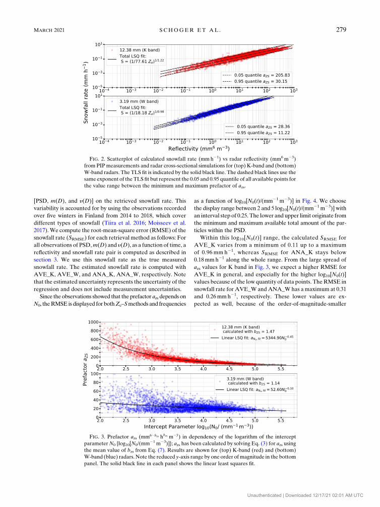
W band we get bzs 5 1.14. The dependency of azs on the in-
tercept parameterN0 is investigated inmore detail. Equation (6)
is solved for azs for each time step with the aforementioned
fixed mean value of bzs and plotted against log10(N0) (see
Fig. 3). Especially for K band, the value range of azs(N0) is on
the order of 102–103. The large scatter of azs at lower N0 values
reduces toward largerN0 values. The prefactor for theW-band
relationship does not show a strong dependency toward N0:
values range from about 10 to 100. A linear least squares fit is
used to approximate a power law for azs[N0(t)] further called
aN0,fit. This method is further called ANA_K and ANA_W for
the analytical relation for K and W band, respectively.
3) UNCERTAINTY ANALYSIS
An uncertainty analysis has been performed to determine
the impact of the natural variability in snowfall properties
FIG. 1. Overview scheme of measured, calculated, and simulated variables needed to re-
trieve the parameters of theZe–S relationship. For the scattering databases utilizing theDDA
method, the following abbreviations are used: Leinonen and Moisseev (2015) (label LM15),
Leinonen and Szyrmer (2015) (label LS15), and Tyynelä and von Lerber (2019) (label
TvL19). All input variables for the retrieval development are displayed in gray. The snowfall
rate retrieved from the in situ data is highlighted in yellow. The colors red and blue are related
to K-band and W-band radar, respectively, and are also used in the following figures to dis-
tinguish between the results from the two radars.
278 JOURNAL OF APPL IED METEOROLOGY AND CL IMATOLOGY VOLUME 60
Unauthenticated | Downloaded 12/17/21 02:01 AM UTC
[PSD, m(D), and y(D)] on the retrieved snowfall rate. This
variability is accounted for by using the observations recorded
over five winters in Finland from 2014 to 2018, which cover
different types of snowfall (Tiira et al. 2016; Moisseev et al.
2017).We compute the root-mean-square error (RMSE) of the
snowfall rate (SRMSE) for each retrieval method as follows: For
all observations of PSD,m(D) and y(D), as a function of time, a
reflectivity and snowfall rate pair is computed as described in
section 3. We use this snowfall rate as the true measured
snowfall rate. The estimated snowfall rate is computed with
AVE_K, AVE_W, and ANA_K, ANA_W, respectively. Note
that the estimated uncertainty represents the uncertainty of the
regression and does not include measurement uncertainties.
Since the observations showed that the prefactor azs depends on
N0, theRMSE is displayed for bothZe–Smethods and frequencies
as a function of log10[N0(t)/(mm21m23)] in Fig. 4. We choose
the display range between 2 and 5 log10[N0(t)/(mm21m23)] with
an interval step of 0.25. The lower and upper limit originate from
the minimum and maximum available total amount of the par-
ticles within the PSD.
Within this log10[N0(t)] range, the calculated SRMSE for
AVE_K varies from a minimum of 0.11 up to a maximum
of 0.96 mm h21, whereas SRMSE for ANA_K stays below
0.18mmh21 along the whole range. From the large spread of
azs values for K band in Fig. 3, we expect a higher RMSE for
AVE_K in general, and especially for the higher log10[N0(t)]
values because of the low quantity of data points. TheRMSE in
snowfall rate for AVE_W andANA_Whas amaximum at 0.31
and 0.26mmh21, respectively. These lower values are ex-
pected as well, because of the order-of-magnitude-smaller
FIG. 2. Scatterplot of calculated snowfall rate (mmh21) vs radar reflectivity (mm6m23)
from PIPmeasurements and radar cross-sectional simulations for (top) K-band and (bottom)
W-band radars. The TLS fit is indicated by the solid black line. The dashed black lines use the
same exponent of the TLS fit but represent the 0.05 and 0.95 quantile of all available points for
the value range between the minimum and maximum prefactor of azs.
FIG. 3. Prefactor azs (mm62bzs hbzs m23) in dependency of the logarithm of the intercept
parameterN0 {log10[N0/(mm21 m23)]}; azs has been calculated by solving Eq. (3) for azs using
the mean value of bzs from Eq. (7). Results are shown for (top) K-band (red) and (bottom)
W-band (blue) radars. Note the reduced y-axis range by one order ofmagnitude in the bottom
panel. The solid black line in each panel shows the linear least squares fit.
MARCH 2021 S CHOGER ET AL . 279
Unauthenticated | Downloaded 12/17/21 02:01 AM UTC

spread in azs values forWband relative toK band in Fig. 3. One
main result of this uncertainty analysis is therefore that
for K band, SRMSE can be strongly reduced when using azs as a
function of N0 (ANA_K), which cannot be seen for W band.
To be able to provide a general uncertainty of our derived
methods, we can directly assign the mean over the considered
log10[N0(t)] for the average Ze–S relationships as both pa-
rameters are constants. For ANA_K and ANA_W, however,
the prefactor a(N0) is different for eachN0, which, on the other
hand, impacts the snowfall-rate uncertainty. Thus, we provide
a first order polynomial regression for the RMSE of S:
SRMSE
[log10(N
0)]5 p
1log
10(N
0)1p
2. (8)
The computed parameters p1 and p2 can be found in Table 1. In
addition, we computed amean value of SRMSE for ANA_K and
ANA_W to directly compare it with the corresponding mean
value of AVE_K and AVE_W. While for AVE_K the mean
value of the SRMSE is around 0.37mm, the mean SRMSE for
ANA_K is only 0.11mmh21. Individual SRMSE values for
ANA_K range from 0.05 to 0.17mmh21 [Eq. (8)] within the
displayed log10[N0(t)] range. The SRMSE mean value for
W-band reflectivities only slightly improves when a(N0) is used
instead of the constant azs. The mean RMSE for ANA_W re-
sults in an uncertainty of 0.16mmh21 and for AVE_W in
0.17mmh21. This marginal improvement does not justify the
higher computational effort of ANA_W. Thus, in the following
application of the new Ze–S relationships, we further use
ANA_K and AVE_W. A summary of all developed Ze–S
relationship parameters as well as their uncertainty values and
functions can be found in Table 1.
b. Application of snowfall-rate retrieval parameters
In this section we apply the developed snowfall-rate re-
trievals from Hyytiälä data to measured reflectivities of the
MiRAC-A and MRR operated at AWIPEV. Especially there,
it is important to have ground-based radar retrieved snowfall
rates considering the scarce ground-based observation net-
work of in situ point-measurements only, as well as the harsh
orographic and weather conditions in the Arctic. As a conse-
quence, Ny-Ålesund could additionally provide improved
ground validation for satellite-based snowfall retrievals at high
latitudes. At AWIPEV, detailed in situ snowfall particle ob-
servations for a retrieval development in Ny-Ålesund are not
available. If Ze–S relationships from the literature are used to
retrieve snowfall at AWIPEV, we need to rely on the as-
sumption that the snow particles at this site match the ones for
which the relationships were originally developed. With our
own relationships we like to emphasize that we do not need to
know the microphysical properties of snow but account for the
variability in snow formation by including the PSD intercept
parameter. Note, that, because of missing MRR and cloud
radar Ze measurements for a same time frame in Hyytiälä, wecould not directly test the relations at this site.
We will demonstrate by means of three case studies that our
new relationships developed fromHyytiälä data work well at a
location, 188 farther north, in the Arctic. First, we evaluate in
detail the retrieved snowfall rate on 7 February 2018 and also
FIG. 4. Uncertainty (RMSE) of the calculated snowfall rate as a function of the intercept
parameter N0 of the particle size distribution. The uncertainty is provided for the average
(dash–dotted) and the analytical Ze–S relationship (solid) for K-band (red) and W-band
(blue) radars, respectively.
TABLE 1. Overview table of calculated parameters azs and bzs from two different methods deriving the Ze–S relationship and the
uncertainty in S for two radar wavelengths. The boldface entries highlight the best parameters used for further evaluation with measured
Ze values.
azs (mm62bzs hbzs m23) bzs SRMSE mean (mmh21) SRMSE[log10(N0)] (mmh21)
AVE_K 77.61 1.22 0.37 —
ANA_K a(N0)5 5344:9N20:450 1.47 0.11 50.04 log10(N0) 2 0.03
(values range from 0.05 to 0.17)
AVE_W 18.18 0.98 0.17 —
ANA_W a(N0)5 52:6N20:10 1.14 0.16 50.04 log10(N0) 2 0.02
(values range from 0.1 to 0.22)
280 JOURNAL OF APPL IED METEOROLOGY AND CL IMATOLOGY VOLUME 60
Unauthenticated | Downloaded 12/17/21 02:01 AM UTC
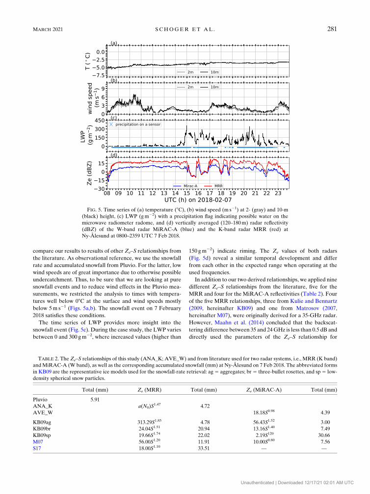
compare our results to results of other Ze–S relationships from
the literature. As observational reference, we use the snowfall
rate and accumulated snowfall from Pluvio. For the latter, low
wind speeds are of great importance due to otherwise possible
undercatchment. Thus, to be sure that we are looking at pure
snowfall events and to reduce wind effects in the Pluvio mea-
surements, we restricted the analysis to times with tempera-
tures well below 08C at the surface and wind speeds mostly
below 5m s21 (Figs. 5a,b). The snowfall event on 7 February
2018 satisfies these conditions.
The time series of LWP provides more insight into the
snowfall event (Fig. 5c). During the case study, the LWP varies
between 0 and 300 gm22, where increased values (higher than
150 gm22) indicate riming. The Ze values of both radars
(Fig. 5d) reveal a similar temporal development and differ
from each other in the expected range when operating at the
used frequencies.
In addition to our two derived relationships, we applied nine
different Ze–S relationships from the literature, five for the
MRR and four for the MiRAC-A reflectivities (Table 2). Four
of the five MRR relationships, three from Kulie and Bennartz
(2009, hereinafter KB09) and one from Matrosov (2007,
hereinafter M07), were originally derived for a 35-GHz radar.
However, Maahn et al. (2014) concluded that the backscat-
tering difference between 35 and 24GHz is less than 0.5 dB and
directly used the parameters of the Ze–S relationship for
FIG. 5. Time series of (a) temperature (8C), (b) wind speed (m s21) at 2- (gray) and 10-m
(black) height, (c) LWP (gm22) with a precipitation flag indicating possible water on the
microwave radiometer radome, and (d) vertically averaged (120–180m) radar reflectivity
(dBZ) of the W-band radar MiRAC-A (blue) and the K-band radar MRR (red) at
Ny-Ålesund at 0800–2359 UTC 7 Feb 2018.
TABLE 2. The Ze–S relationships of this study (ANA_K; AVE_W) and from literature used for two radar systems, i.e., MRR (K band)
andMiRAC-A (W band), as well as the corresponding accumulated snowfall (mm) at Ny-Ålesund on 7 Feb 2018. The abbreviated forms
in KB09 are the representative ice models used for the snowfall-rate retrieval: ag5 aggregates; br5 three-bullet rosettes, and sp5 low-
density spherical snow particles.
Total (mm) Ze (MRR) Total (mm) Ze (MiRAC-A) Total (mm)
Pluvio 5.91
ANA_K a(N0)S1.47 4.72
AVE_W 18.18S0.98 4.39
KB09ag 313.29S1.85 4.78 56.43S1.52 3.00
KB09br 24.04S1.51 20.94 13.16S1.40 7.49
KB09sp 19.66S1.74 22.02 2.19S120 30.66
M07 56.00S1.20 11.91 10.00S0.80 7.56
S17 18.00S1.10 33.51 — —
MARCH 2021 S CHOGER ET AL . 281
Unauthenticated | Downloaded 12/17/21 02:01 AM UTC

35GHz to retrieve snowfall rate from MRR reflectivities. An
actual relationship for the 24-GHz MRR has recently been
derived by S17 who also used a PIP instrument, but at the
Princess Elisabeth Station in East Antarctica, where snow
particles are smaller than at northern midlatitudes. KB09 and
M07 also derived Ze–S relationships for 94GHz radars, which
we applied to the MiRAC-A reflectivities.
To differentiate between the different relationships for the
different frequencies, we use the notation, for example,M07_K
and M07_W, to indicate which Ze–S relationship is applied to
MRR and MiRAC-A reflectivities, respectively. Furthermore,
since KB09 derived three relations for different particle shapes
from idealized models that represent unrimed ice particles best
and thus dry snowfall, we abbreviate the various ice particle
models used in KB09 as follows: aggregates (KB09ag), three-
bullet rosettes (KB09br), and low-density spherical snow par-
ticles (KB09sp). M07 derived the Ze–S relationships from
nonspherical aggregate and single crystal dendrite snow par-
ticle models for dry snowfall. The dataset from Hyytiälä con-
sists of a mixture of snow particles, that is, single crystals, low
density, and rimed aggregates. Meteorological conditions seem
to favor riming process in Hyytiälä when derived snowfall
masses are compared to model simulations (Tyynelä and von
Lerber 2019). Moisseev et al. (2017) demonstrated during the
winter of 2014/15 that riming is responsible for 5%–40% of
snowfall mass.
The values of the prefactor azs for our derived relationship
ANA_K differ between 59.25 and 2119.06 with a mean of
318.65. In comparison with the relationships from the literature
applied toMRR reflectivities the azs values differ only between
18 and 313. The instantaneous values of azs throughout the day
can be seen in Fig. 6 and show a large fluctuation especially for
the times when we generally have more liquid water in the
atmosphere (between 1500 and 2300 UTC). These swings are a
physical signal, as they describe the large changes in N0. This
large spread in azs values underlines the need for a changing
parameter rather than a constant prefactor. The latter does not
capture the variability of the snowfall properties, which vary
with time.
The application of the different Ze–S relationships from the
literature results in large variations in snowfall rate for the
present case study (Figs. 7a). The accumulated snowfall from
all relationships during this day ranges between 3 and 33mm
(Figs. 7b) with the total accumulation amounts listed in
Table 2. One would have expected that the relationships from
the literature for the same particle types, but different fre-
quencies would result in a similar snowfall rate. For example,
the time series of the snowfall rate as well as of the accumu-
lated snowfall until about 1900 UTC reveal that the relations
by S17_K and KB09sp_W agree surprisingly well, but the ac-
cumulation calculated with KB09sp_K has 8.64mm less than
the amount of KB09sp_W. If we take Pluvio as the observa-
tional reference for the snow accumulation, most of the rela-
tionships from the literature show a far too high accumulated
snowfall (up to almost 30mm difference).
To have a closer look on the derived relationships in this
study we compare them to the relationships from the literature
that fitmore closely toPluviomeasurements, namelyKB09ag_K
and KB09ag_W. An enlarged view onto these four rela-
tionships can be seen in Fig. 8. The temporal developments of
the snowfall rate computed with ANA_K and AVE_W agree
very well with each other within their displayed uncertainty
range. Also, the snowfall rates fromKB09ag_K and KB09ag_W
are most of the time within this uncertainty range. With
regard to the snowfall accumulation, the amount between
ANA_K and AVE_W differs by 0.33mm, only, whereas
KB09ag_K and KB09ag_W differ by 1.78mm. Relative to
Pluvio, KB09ag_K shows the smallest difference of 1.13mm
(19%). ANA_K and AVE_W have a difference of 1.19mm
(20%) and 1.52mm (25%), respectively, and KB09ag_W
shows the largest difference of 2.91mm (49%). From this case
study, we can draw several conclusions: First, we show that the
geographical differences in the radar-based snowfall intensity
estimates, often reported in the literature, can be reduced by
taking into account changes in the PSD intercept parameter
N0. Therefore, a combination of a radar and a disdrometer can
be used for quantitative snowfall measurements and retrievals.
The retrieval method is not too sensitive to a geographical
location. This is demonstrated by developing Ze–S relations
using data from Hyytiälä and applying them to the observa-
tions at Ny-Ålesund. We also show that the uncertainty of Ze–
S-based snowfall estimates depend on radar frequency. For
snowfall intensity estimates based on W-band radar observa-
tions, the Ze–S relation adjustment by using the PSD intercept
FIG. 6. Time series of the instantaneous prefactor azs (mm62bzs hbzs m23) of the analyticalZe–S
relationship for the MRR for the case study at Ny-Ålesund on 7 Feb 2018.
282 JOURNAL OF APPL IED METEOROLOGY AND CL IMATOLOGY VOLUME 60
Unauthenticated | Downloaded 12/17/21 02:01 AM UTC

parameter seems to be unnecessary. Furthermore, it is shown
that by comparing snowfall intensity estimates using data from
radars operating at different frequencies, that is, K and W
band, potential instrumental errors can be diagnosed. To
achieve this, however, the snowfall rate calculated with Ze–S
relations for different radar frequencies should be consistent
between each other, that is, relying on the same assumptions and
retrieval uncertainties should also be known. It appears that the
Ze–S relationships from the literature, at least those discussed in
this study, show a large variability and are not necessarily con-
sistent with each other throughout the used frequency range,
even when the same particle type assumption is used.
To gain a higher confidence in our method, we analyzed two
further case studies for Ny-Ålesund for 16 March and 16 April
2018 (Figs. 9–12, Table 3). Also for these cases, ANA_K and
AVE_W show a similar temporal development of the snowfall
rate and agree very well within their uncertainty range. Their
accumulation difference to the observational reference Pluvio
is small: on 16March 2018, the differences are10.73mm (36%)
for AVE_W and 11.84mm (92%) for ANA_K (Fig. 10). On
16 April 2018, the snowfall accumulation is underestimated by
0.35mm(19%)by 0.35mm(19%)byANA_Kand 0.54mm(29%)
by AVE_W (Fig. 12). The closest relationships from the literature
are similar as for 7 February 2018, KB09ag_K and KB09ag_W as
well asM07_W (Table 3). The difference of snowfall amounts from
the otherZe–S relationships from the literature compared to Pluvio
are much higher. They overestimate the snowfall accumulation by
2–20mm (100%–992%) on 16 March and by 0.8–9mm (43%–
476%) on 16 April 2018.
S17 and KB09sp_W are in all case studies the two relation-
ships that show the largest differences in snowfall accumula-
tion compared to Pluvio. Note that temperature, wind speed,
and LWP are different for both days (Figs. 10 and 11). For
16 March 2018, temperatures are well below zero and LWP is
much lower than for 7 February 2018. The wind speeds are less
than 3m s21 throughout most of the day with values of up to
10m s21 at the beginning and end of the day. The latter could
have led to a delayed onset of snowfall detection by Pluvio that
can be seen in the accumulated snowfall (Fig. 10).Nevertheless, as
mentioned before, differences between snowfall amounts of
Pluvio and of ANA_K and AVE_W are small compared to most
of the differences in snowfall amount related to the various Ze–S
relationships from the literature. On 16 April 2018, temperatures
are just above 08C and thus higher compared to the other two
cases. The wind speed is very low, with values below 2ms21 most
of the time. For completeness, the azs values (not shown)
for K band ranged between 31 and 1235 with a mean of 215 on
16 March 2018. On 16 April 2018, azs values range from 103 to
1898 with a mean of 340.
5. Summary and outlook
Two Ze–S relationships for K- and W-band radars, respec-
tively, have been developed in this study. For the W-band
FIG. 7. (a) Snowfall rate (mmh21) at Ny-Ålesund on 7 Feb 2018 from the two methods
developed in this study for the W-band radar MiRAC-A (AVE_W) and for the K-band radar
MRR (ANA_K), as well as nineZe–S relationships from the literature—five forMRR and four
for MiRAC-A. The abbreviated forms in KB09 are the representative ice models used for the
snowfall-rate retrieval: ag 5 aggregates; br 5 three-bullet rosettes, and sp 5 low-density
spherical snow particles for K-band and W-band radar, indicated by _K or _W, respectively.
(b) Accumulated snowfall (mm) from the same relationships as in (a) and additionally from the
observational reference Pluvio.
MARCH 2021 S CHOGER ET AL . 283
Unauthenticated | Downloaded 12/17/21 02:01 AM UTC

radar, a common approach with constant parameters, here
called average relationship, is applied. For the K-band radar,
we used an analytical method in which the prefactor azs is kept
variable in time and depends on the PSD intercept parameter
N0. This method is new and has not been applied yet for
snowfall-rate retrievals.
Especially at higher latitudes and in theArctic due to its fast-
changing climate, the observation of snowfall is crucial to ex-
amine. Surface instrumentation such as a precipitation gauge is
prone to undercatchment and theW-band radar on the satellite
CloudSat is unreliable within its blind zone (closest 1200m
toward the ground) (Maahn et al. 2014), where some of the
FIG. 9. As in Fig. 5, but for 0000–2359 UTC 16 Mar 2018.
FIG. 8. As in Fig. 7, but zooming in on the methods developed in this study. The uncertainty
of the snowfall rate of AVE_W and ANA_K is indicated by the blue and red shading, re-
spectively. Two relationships from the literature, i.e., KB09ag_K and KB09ag_W, are shown
as well (see caption of Fig. 7 for further details).
284 JOURNAL OF APPL IED METEOROLOGY AND CL IMATOLOGY VOLUME 60
Unauthenticated | Downloaded 12/17/21 02:01 AM UTC

shallow snowfall is forming (Kulie et al. 2016; Kulie and
Milani 2018).
The ground-based MRR, measuring in the K band, is more
and more used at different sites including Antarctica and has
recently been installed at the AWIPEV Arctic Research Base
in Ny-Ålesund together with theW-band cloud radarMiRAC-A.
In this study, we introduced a method with which it is possi-
ble to operationally retrieve snowfall rates from MRR mea-
surements. Additionally, we can increase the confidence in the
MRR retrieved snowfall rates by comparing them to snowfall
rates retrieved from the reflectivities of the parallel in time
operating MiRAC-A and to Pluvio measurements. We use the
Pluvio as the in situ observational reference. To develop Ze–S
relationships, detailed in situ observations of snowfall particles are
needed, which are unfortunately not available at AWIPEV. We
have thus used snowfall measurements (fall velocity, particle size
distribution, and mass) from the video-disdrometer PIP at the
measurement site in Hyytiälä, Finland. With these variables we
FIG. 10. As in Fig. 8, but for 0000–2359 UTC 16 Mar 2018.
FIG. 11. As in Fig. 5, but for 1000–1730 UTC 16 Apr 2018.
MARCH 2021 S CHOGER ET AL . 285
Unauthenticated | Downloaded 12/17/21 02:01 AM UTC

were able to calculate snowfall rates and simulate reflectivity
values at K and W band, respectively. Based on this dataset,
the two different Ze–S relationships, that is, the more
common approach with constant parameters and the new
analytical approach with time- and N0-dependent prefactor
azs, were developed.
An uncertainty analysis revealed that the new approach
strongly reduces the uncertainty for snowfall rates calculated
with K-band reflectivities by more than half, from 0.37 to
0.11mmh21. The uncertainty for the snowfall rates from the
W-bandZe–S relationships only differed by 0.01mmh21. Thus,
for W band, the average Ze–S relationship is favored over the
more complex analytical Ze–S relationship.
To test the performance of the developed relationships, we
applied the analytical Ze–S relationship to measured re-
flectivity values of the MRR (ANA_K) and the average Ze–S
relationship to MiRAC-A reflectivities (AVE_W) in Ny-Åle-
sund for a case study on 7 February 2018. Low wind conditions
on this day facilitated a comparison of the snowfall accumu-
lation from the radar with the precipitation gauge Pluvio. In
addition, we compared snowfall rates retrieved with different
Ze–S relationships from literature with the snowfall rates cal-
culated from our methods.
A large spread in the total accumulated snowfall values of
the Ze–S relationships from the literature shows the difficulty
of just applying any Ze–S relationship to reflectivity values at
any location. Our results show that a relationship that has been
developed for Antarctica (S17) might not be appropriate for
the Arctic site in Ny-Ålesund. The Ze–S relationship (S17)
revealed the largest differences in snowfall rate and snowfall
accumulation (about 30mm) relative to Pluvio and our de-
velopedmethods. One possible reason for this difference could
be that particle types and also the PSD in Antarctica are quite
different to the particle types and PSD in Ny-Ålesund.
However, more detailed information on particle masses and
types of the snowfall would be needed at Ny-Ålesund to have a
closer look on the snow characteristics.
For the case study analyzed, we could show that the newly
developedZe–S relationships ANA_K andAVE_W agree well
with the observational reference and also well with each other
within their uncertainty range. The accumulated snowfall on
7 February 2018 derived with ANA_K and AVE_W is only
1.19mm (20%) and 1.52mm (25%), respectively, less than the
accumulated snowfall amount from Pluvio (5.91mm). This
matching also indicates that the snowfall conditions at Ny-
Ålesund are likely similar to the ones at Hyytiälä. When in-
cluding further Ze–S relationships from literature in the anal-
ysis, the corresponding retrieved accumulated snowfall values
differ from the Pluvio snowfall amount by 19%–467%. Only
two of the applied relationships from the literature, that is,
KB09ag_K and KB09ag_W, show a similar good performance
as ANA_K and AVE_W.
FIG. 12. As in Fig. 8, but for 1000–1730 UTC 16 Apr 2018.
TABLE 3. Accumulated snowfall (mm) at Ny-Ålesund on
16 Mar and 16 Apr 2018 from the observational reference
Pluvio and from the sameZe–S relationships as shown in Table 2
using MRR (K band) and MiRAC-A (W band) reflectivity
measurements.
16 Mar 2018 16 Apr 2018
MRR MiRAC-A MRR MiRAC-A
Pluvio 2.01 1.88
ANA_K 3.86 1.34
AVE_W 2.74 1.53
KB09ag 3.63 2.47 1.63 1.10
KB09br 14.08 5.88 6.78 2.70
KB09sp 16.16 21.95 7.40 10.84
M07 6.84 4.04 3.63 2.63
S17 18.04 9.97
286 JOURNAL OF APPL IED METEOROLOGY AND CL IMATOLOGY VOLUME 60
Unauthenticated | Downloaded 12/17/21 02:01 AM UTC
An analysis of two further case studies at Ny-Ålesund with
different meteorological conditions also showed good results
for both the temporal development of the snowfall rate as well
as the snowfall accumulation relative to the observational
reference. An analysis of a longer time period of snowfall
measurements is necessary to be able to provide more robust
statistics and will be one of the next steps. The application to
the long-term data at Ny-Ålesund, however, is difficult and
bears other uncertainties such as the discrimination between
liquid and solid precipitation in the first place and using addi-
tional correction equations for Pluvio to account for precipi-
tation losses in high wind conditions.
In addition to the application of the newly developed Ze–S
relationships to the measurements at Ny-Ålesund, also the
MRR measurements as part of the Cold-Air Outbreaks in the
Marine Boundary Layer Experiment (COMBLE; December
2019–May 2020) on Bear Island, Svalbard, will be analyzed in
more detail and snowfall rates estimated. In this way, we
will gain further insight into the spatial variability of precipi-
tation in Svalbard and also show the broader applicability of
our method. In this respect, we have also recently applied the
newly developed K-band Ze–S relationship to measurements
of a site in Marquette, Michigan, where MRR measurements
with collocated PIP observations were available (Pettersen
et al. 2020). Those results (not shown) are promising and will
be investigated in more detail in the future.
Acknowledgments We gratefully acknowledge the funding
by the Deutsche Forschungsgemeinschaft (DFG, German
Research Foundation)—Project-ID 268020496–TRR 172, within
the Transregional Collaborative Research Center Arctic
Amplification: Climate Relevant Atmospheric and Surface
Processes, and Feedback Mechanisms (AC)3. We thank the
AWIPEV team for their support in the operation of our
instruments at AWIPEV and Christoph Ritter for providing
the HATPRO measurements. We thank the personnel of
Hyytiälä station and Matti Leskinen for their support in
field observation. We appreciate the comments by the three
anonymous reviewers.
Data availability statement. The meteorological surface
BSRN observations are available from PANGAEA (Maturilli
2018). The MWR LWP data can also be downloaded from
PANGAEA (Nomokonova et al. 2019b). The first two years of
the PIP data are available at https://zenodo.org/record/3977959
(Moisseev 2020). TheMRR,MiRAC-A, Pluvio, and PARSIVEL
measurements of the case studies are available at https://doi.org/
10.5281/zenodo.4017348 (Ebell 2020).
REFERENCES
Battaglia, A., E. Rustemeier, A. Tokay, U. Blahak, and C. Simmer,
2010: PARSIVEL snow observations: A critical assessment.
J. Atmos. Oceanic Technol., 27, 333–344, https://doi.org/
10.1175/2009JTECHA1332.1.
Boggs, P. T., and J. E. Rogers, 1990: Orthogonal distance regres-
sion. Statistical Analysis of Measurement Error Models and
Applications: Proc. AMS-IMS-SIAM Joint Summer Research
Conf., Arcata, CA, American Mathematical Society, 183–194.
——, R. H. Byrd, J. E. Rogers, and R. B. Schnabel, 1992: User’s
reference guide for ODRPACK version 2.01: Software for
weighted orthogonal distance regression. Accessed 30 August
2019, https://docs.scipy.org/doc/external/odrpack_guide.pdf.
Bruggeman, D. A. G., 1935: Berechnung verschiedener phys-
ikalischer Konstanten von heterogenen Substanzen. I.
Dielektrizitätskonstanten und Leitfähigkeiten der Mischkörperaus isotropen Substanzen. Ann. Phys., 416, 636–664, https://
doi.org/10.1002/andp.19354160705.
Carlson, P. E., and J. S. Marshall, 1972: Measurement of snowfall
by radar. J. Appl. Meteor., 11, 494–500, https://doi.org/10.1175/
1520-0450(1972)011,0494:MOSBR.2.0.CO;2.
Chase, R. J., S. W. Nesbitt, and G. M. McFarquhar, 2020:
Evaluation of the microphysical assumptions within GPM-
DPR using ground-based observations of rain and snow.
Atmosphere, 11, 619, https://doi.org/10.3390/atmos11060619.
Ebell, K., 2020: Cloud radar, Micro Rain Radar, Parsivel and
Pluvio measurements at Ny-Ålesund for 7 Feb 2018, 16March
2018 and 16 April 2018. Zenodo, https://doi.org/10.5281/
zenodo.4017348.
Falconi, M. T., A. Lerber, D. Ori, F. S. Marzano, and D. Moisseev,
2018: Snowfall retrieval at X, Ka andW bands: Consistency of
backscattering and microphysical properties using BAECC
ground-based measurements. Atmos. Meas. Tech., 11, 3059–
3079, https://doi.org/10.5194/amt-11-3059-2018.
Førland, E. J., R. Benestad, I. Hanssen-Bauer, J. E. Haugen, and
T. E. Skaugen, 2011: Temperature and precipitation devel-
opment at Svalbard 1900-2100. Adv. Meteor., 2011, 893790,
https://doi.org/10.1155/2011/893790.
Fujiyoshi, Y., T. Endoh, T. Yamada, K. Tsuboki, Y. Tachibana, and
G. Wakahama, 1990: Determination of a Z–R relationship for
snowfall using a radar and high sensitivity snow gauges.
J. Appl. Meteor., 29, 147–152, https://doi.org/10.1175/1520-
0450(1990)029,0147:DOARFS.2.0.CO;2.
Hari, P., and M. Kulmala, 2005: Station for Measuring Ecosystem-
Atmosphere Relations: SMEAR. Boreal Environ. Res., 10,
315–322.
Heymsfield, A. J., S. Y. Matrosov, and N. B. Wood, 2016: Toward
improving ice water content and snow-rate retrievals from
radars. Part I: X andW bands, emphasizing CloudSat. J. Appl.
Meteor. Climatol., 55, 2063–2090, https://doi.org/10.1175/
JAMC-D-15-0290.1.
Huang, G.-J. J., V. N. Bringi, R. Cifelli, D. Hudak, and W. A.
Petersen, 2010: A methodology to derive radar reflectivity-
liquid equivalent snow rate relations using C-band radar and a
2D video disdrometer. J. Atmos. Oceanic Technol., 27, 637–
651, https://doi.org/10.1175/2009JTECHA1284.1.
IPCC, 2007: Climate Change 2007: The Physical Science Basis.
Cambridge University Press, 996 pp.
Klugmann, D., K. Heinsohn, and H. J. Kirtzel, 1996: A low cost
24GHz FM-CW Doppler radar rain profiler. Contrib. Atmos.
Phys., 69, 247–253.
Kneifel, S.,M.Maahn,G. Peters, andC. Simmer, 2011:Observation of
snowfall with a low-power FM-CW K-band radar (Micro Rain
Radar).Meteor. Atmos. Phys., 113, 75–87, https://doi.org/10.1007/
s00703-011-0142-z.
——, A. Lerber, J. Tiira, D. Moisseev, P. Kollias, and J. Leinonen,
2015: Observed relations between snowfall microphysics and
triple-frequency radar measurements. J. Geophys. Res. Atmos.,
120, 6034–6055, https://doi.org/10.1002/2015JD023156.
Kollias, P., E. E. Clothiaux, M. A. Miller, B. A. Albrecht, G. L.
Stephens, and T. P. Ackerman, 2007: Millimeter-wavelength
radars: New frontier in atmospheric cloud and precipitation
MARCH 2021 S CHOGER ET AL . 287
Unauthenticated | Downloaded 12/17/21 02:01 AM UTC

research. Bull. Amer. Meteor. Soc., 88, 1608–1624, https://
doi.org/10.1175/BAMS-88-10-1608.
Küchler, N., S. Kneifel, U. Löhnert, P. Kollias, H. Czekala, and
T. Rose, 2017: A W-band radar-radiometer system for accu-
rate and continuous monitoring of clouds and precipitation.
J. Atmos. Oceanic Technol., 34, 2375–2392, https://doi.org/
10.1175/JTECH-D-17-0019.1.
Kulie, M. S., and R. Bennartz, 2009: Utilizing spaceborne radars to
retrieve dry snowfall. J. Appl. Meteor. Climatol., 48, 2564–
2580, https://doi.org/10.1175/2009JAMC2193.1.
——, and L. Milani, 2018: Seasonal variability of shallow cumuli-
form snowfall: A CloudSat perspective.Quart. J. Roy. Meteor.
Soc., 144, 329–343, https://doi.org/10.1002/qj.3222.——, ——, N. B. Wood, S. A. Tushaus, R. Bennartz, and T. S.
L’Ecuyer, 2016: A shallow cumuliform snowfall census using
spaceborne radar. J. Hydrometeor., 17, 1261–1279, https://
doi.org/10.1175/JHM-D-15-0123.1.
Langille, R. C., and R. S. Thain, 1951: Some quantitative mea-
surements of three-centimeter radar echoes from falling snow.
Can. J. Phys., 29, 482–490, https://doi.org/10.1139/p51-052.
Leinonen, J., 2014: High-level interface to T-matrix scattering
calculations: Architecture, capabilities and limitations. Opt.
Express, 22, 1655–1660, https://doi.org/10.1364/OE.22.001655.
——, 2018: Python code for T-matrix scattering calculations.
Accessed 24 August 2018, https://github.com/jleinonen/pytmatrix/.
——, and D. Moisseev, 2015: What do triple-frequency radar sig-
natures reveal about aggregate snowflakes? J. Geophys. Res.
Atmos., 120, 229–239, https://doi.org/10.1002/2014JD022072.
——, andW. Szyrmer, 2015: Radar signatures of snowflake riming:
Amodeling study.Earth Space Sci., 2, 346–358, https://doi.org/
10.1002/2015EA000102.
——, S. Kneifel, D. Moisseev, J. Tyynelä, S. Tanelli, and
T. Nousiainen, 2012: Evidence of nonspheroidal behavior
in millimeter-wavelength radar observations of snowfall.
J. Geophys. Res., 117, D18205, https://doi.org/10.1029/
2012JD017680.
——, and Coauthors, 2018: Retrieval of snowflake microphysical
properties frommultifrequency radar observations.Atmos.Meas.
Tech., 11, 5471–5488, https://doi.org/10.5194/amt-11-5471-2018.
Levizzani, V., S. Laviola, and E. Cattani, 2011: Detection and
measurement of snowfall from space. Remote Sens., 3, 145–
166, https://doi.org/10.3390/rs3010145.
Lhermitte, R., 1987: A 94-GHz doppler radar for cloud observa-
tions. J. Atmos. Oceanic Technol., 4, 36–48, https://doi.org/
10.1175/1520-0426(1987)004,0036:AGDRFC.2.0.CO;2.
——, 1988: Observation of rain at vertical incidence with a 94GHz
Doppler radar: An insight onMie scattering.Geophys. Res. Lett.,
15, 1125–1128, https://doi.org/10.1029/GL015i010p01125.
Li, H., D. Moisseev, and A. von Lerber, 2018: How does riming
affect dual-polarization radar observations and snowflake
shape? J. Geophys. Res. Atmos., 123, 6070–6081, https://
doi.org/10.1029/2017JD028186.
López-Moreno, J. I., J. Boike, A. Sanchez-Lorenzo, and J. W.
Pomeroy, 2016: Impact of climate warming on snow pro-
cesses in Ny-Ålesund, a polar maritime site at Svalbard.
Global Planet. Change, 146, 10–21, https://doi.org/10.1016/
j.gloplacha.2016.09.006.
Maahn,M., and P. Kollias, 2012: ImprovedMicroRainRadar snow
measurements using Doppler spectra post-processing. Atmos.
Meas. Tech., 5, 2661–2673, https://doi.org/10.5194/amt-5-2661-
2012.
——, C. Burgard, S. Crewell, I. V. Gorodetskaya, S. Kneifel,
S. Lhermitte, K. Van Tricht, and N. P. M. van Lipzig, 2014:
How does the spaceborne radar blind zone affect derived
surface snowfall statistics inpolar regions? J.Geophys.Res.Atmos.,
119, 13 604–13620, https://doi.org/10.1002/2014JD022079.
Mason, S. L., C. J. Chiu, R. J. Hogan, D. Moisseev, and S. Kneifel,
2018: Retrievals of riming and snow density from vertically
pointingDoppler radars. J. Geophys. Res. Atmos., 123, 13 807–
13 834, https://doi.org/10.1029/2018JD028603.
——, R. J. Hogan, C. D. Westbrook, S. Kneifel, D. Moisseev, and
L. von Terzi, 2019: The importance of particle size distribution
and internal structure for triple-frequency radar retrievals of
the morphology of snow. Atmos. Meas. Tech., 12, 4993–5018,
https://doi.org/10.5194/amt-12-4993-2019.
Matrosov, S. Y., 2007: Modeling backscatter properties of snowfall
at millimeter wavelengths. J. Atmos. Sci., 64, 1727–1736,
https://doi.org/10.1175/JAS3904.1.
——, M. D. Shupe, and I. V. Djalalova, 2008: Snowfall retrievals
using millimeter-wavelength cloud radars. J. Appl. Meteor.
Climatol., 47, 769–777, https://doi.org/10.1175/2007JAMC1768.1.
Maturilli, M., 2018: Continuous meteorological observations at
station Ny-Ålesund (2018-02). PANGAEA, accessed 1 June
2019, https://doi.org/10.1594/PANGAEA.894665.
——, A. Herber, and G. König-Langlo, 2013: Climatology and time
series of surface meteorology in Ny-Ålesund, Svalbard.Earth Syst.
Sci. Data, 5, 155–163, https://doi.org/10.5194/essd-5-155-2013.
Mech, M., L.-L. Kliesch, A. Anhäuser, T. Rose, P. Kollias, and
S. Crewell, 2019: Microwave Radar/Radiometer for Arctic
Clouds (MiRAC): First insights from the ACLOUD cam-
paign. Atmos. Meas. Tech., 12, 5019–5037, https://doi.org/
10.5194/amt-12-5019-2019.
Mishchenko, M. I., and L. D. Travis, 1994: T-matrix computa-
tions of light scattering by large spheroidal particles. Opt.
Commun., 109, 16–21, https://doi.org/10.1016/0030-4018(94)
90731-5.
Mitchell, D. L., and A. J. Heymsfield, 2005: Refinements in the
treatment of ice particle terminal velocities, highlighting ag-
gregates. J. Atmos. Sci., 62, 1637–1644, https://doi.org/10.1175/
JAS3413.1.
Moisseev, D., 2020: dmoisseev/Snow-Retrievals-2014-2015: Snowfalke
mass retrievals 2014/2015. Zenodo, https://doi.org/10.5281/
zenodo.3977959.
——, and V. Chandrasekar, 2007: Examination of the m-L.J. Atmos. Oceanic Technol., 24, 847–855, https://doi.org/
10.1175/JTECH2010.1.
——, A. von Lerber, and J. Tiira, 2017: Quantifying the effect of
riming on snowfall using ground-based observations. J. Geophys.
Res.Atmos., 122, 4019–4037, https://doi.org/10.1002/2016JD026272.
Newman,A. J., P. A. Kucera, and L. F. Bliven, 2009: Presenting the
Snowflake Video Imager (SVI). J. Atmos. Oceanic Technol.,
26, 167–179, https://doi.org/10.1175/2008JTECHA1148.1.
Nomokonova, T., K. Ebell, U. Löhnert,M.Maturilli, C. Ritter, and
E. O’Connor, 2019a: Statistics on clouds and their relation to
thermodynamic conditions at Ny-Ålesund using ground-based
sensor synergy. Atmos. Chem. Phys. Discuss., 19, 4105–4126,
https://doi.org/10.5194/acp-19-4105-2019.
——, C. Ritter, and K. Ebell, 2019b: HATPRO microwave radi-
ometer measurements at AWIPEV, Ny-Ålesund (2016-2018).
PANGAEA, accessed 1 June 2019, https://doi.org/10.1594/
PANGAEA.902183.
OTT, 2016: Operating instructions: Precipitation gauge OTT
Pluvio2L. OTT Doc., 60 pp., https://www.ott.com/download/
operating-instructions-precipitation-gauge-ott-pluvio2-l-1/.
Pettersen, C., and Coauthors, 2020: The precipitation imaging
package:Assessment ofmicrophysical and bulk characteristics
288 JOURNAL OF APPL IED METEOROLOGY AND CL IMATOLOGY VOLUME 60
Unauthenticated | Downloaded 12/17/21 02:01 AM UTC

of snow. Atmosphere, 11, 785, https://doi.org/10.3390/
atmos11080785.
Rasmussen, R., M. Dixon, S. Vasiloff, F. Hage, S. Knight,
J. Vivekanandan, and M. Xu, 2003: Snow nowcasting using a
real-time correlation of radar reflectivity with snow gauge
accumulation. J. Appl. Meteor., 42, 20–36, https://doi.org/
10.1175/1520-0450(2003)042,0020:SNUART.2.0.CO;2.
——, and Coauthors, 2012: How well are we measuring snow: The
NOAA/FAA/NCAR winter precipitation test bed. Bull.
Amer. Meteor. Soc., 93, 811–829, https://doi.org/10.1175/
BAMS-D-11-00052.1.
Rasmussen, R. M., S. Landolt, B. Baker, J. Kochendorfer,
B. Collins, M. Colli, L. Lanza, and J. Theriault, 2014:
Examination of the performance of single Alter shielded and
unshielded snow gauges using observations from the Marshall
Field Site during the SPICE WMO Field Program and nu-
merical model simulations. 17th Symp. on Meteorological
Observation and Instrumentation, Westminster, CO, Amer.
Meteor. Soc., 2.4, https://ams.confex.com/ams/21Applied17SMOI/
webprogram/Paper247562.html.
Rose, T., S. Crewell, U. Löhnert, and C. Simmer, 2005: A network
suitable microwave radiometer for operational monitoring of
the cloudy atmosphere. Atmos. Res., 75, 183–200, https://
doi.org/10.1016/j.atmosres.2004.12.005.
Schrom, R. S., and M. R. Kumjian, 2018: Bulk-density represen-
tations of branched planar ice crystals: Errors in the polari-
metric radar variables. J. Appl. Meteor. Climatol., 57, 333–346,
https://doi.org/10.1175/JAMC-D-17-0114.1.
Serreze, M. C., and R. G. Barry, 2011: Processes and impacts of
Arctic amplification: A research synthesis. Global Planet.
Change, 77, 85–96, https://doi.org/10.1016/j.gloplacha.2011.
03.004.
Sihvola, A., 1999:ElectromagneticMixing Formulas and Applications.
Institution of Electrical Engineers, 296 pp.
Souverijns, N., A. Gossart, S. Lhermitte, I. V. Gorodetskaya,
S. Kneifel,M.Maahn, F. L. Bliven, andN. P.M.M. van Lipzig,
2017: Estimating radar reflectivity–snowfall rate relationships
and their uncertainties over Antarctica by combining dis-
drometer and radar observations. Atmos. Res., 196, 211–223,
https://doi.org/10.1016/j.atmosres.2017.06.001.
Stephens, G. L., and Coauthors, 2002: The CloudSat mission and
the A-train. Bull. Amer. Meteor. Soc., 83, 1771–1790, https://
doi.org/10.1175/BAMS-83-12-1771.
——, D. Winker, J. Pelon, C. Trepte, D. Vane, C. Yuhas,
T. L’Ecuyer, and M. Lebsock, 2018: CloudSat and CALIPSO
within the A-train: Ten years of actively observing the Earth
system. Bull. Amer. Meteor. Soc., 99, 569–581, https://doi.org/
10.1175/BAMS-D-16-0324.1.
Tiira, J., D. N. Moisseev, A. von Lerber, D. Ori, A. Tokay, L. F.
Bliven, andW. Petersen, 2016: Ensemble mean density and its
connection to othermicrophysical properties of falling snow as
observed in southern Finland. Atmos. Meas. Tech., 9, 4825–
4841, https://doi.org/10.5194/amt-9-4825-2016.
Tyynelä, J., and A. von Lerber, 2019: Validation of microphysical
snow models using in situ, multifrequency, and dual-
polarization radar measurements in Finland. J. Geophys.
Res. Atmos., 124, 13 273–13 290, https://doi.org/10.1029/
2019JD030721.
——, J. Leinonen, D. Moisseev, and T. Nousiainen, 2011: Radar
backscattering from snowflakes: Comparison of fractal, ag-
gregate, and soft spheroidmodels. J. Atmos. Oceanic Technol.,
28, 1365–1372, https://doi.org/10.1175/JTECH-D-11-00004.1.
Ulbrich, C.W., andD.Atlas, 1998: Rainfall microphysics and radar
properties: Analysis methods for drop size spectra. J. Appl.
Meteor., 37, 912–923, https://doi.org/10.1175/1520-0450(1998)037,0912:RMARPA.2.0.CO;2.
von Lerber, A., D. Moisseev, L. F. Bliven, W. Petersen, A.-M. M.
Harri, andV. Chandrasekar, 2017:Microphysical properties of
snow and their link to Ze–S relations during BAECC 2014.
J. Appl. Meteor. Climatol., 56, 1561–1582, https://doi.org/
10.1175/JAMC-D-16-0379.1.
——, ——, D. A. Marks, W. Petersen, A.-M. Harri, and
V. Chandrasekar, 2018: Validation of GMI snowfall ob-
servations by using a combination of weather radar and
surface measurements. J. Appl. Meteor. Climatol., 57, 797–
820, https://doi.org/10.1175/JAMC-D-17-0176.1.
Wendisch,M., and Coauthors, 2017: Understanding causes and effects
of rapid warming in the Arctic. Eos, Trans. Amer. Geophys.
Union, 98, 22–26, https://doi.org/10.1029/2017EO064803.
——, and Coauthors, 2018: The Arctic cloud puzzle: Using
ACLOUD/PASCAL multi-platform observations to unravel
the role of clouds and aerosol particles in Arctic amplification.
Bull. Amer. Meteor. Soc., 100, 841–871, https://doi.org/
10.1175/BAMS-D-18-0072.1.
Yurkin, M. A., and A. G. Hoekstra, 2011: The discrete-dipole-
approximation code ADDA: Capabilities and known limita-
tions. J. Quant. Spectrosc. Radiat. Transfer, 112, 2234–2247,https://doi.org/10.1016/j.jqsrt.2011.01.031.
Zawadzki, I., E. Jung, and G. Lee, 2010: Snow studies. Part I: A
study of natural variability of snow terminal velocity.
J. Atmos. Sci., 67, 1591–1604, https://doi.org/10.1175/
2010JAS3342.1.
MARCH 2021 S CHOGER ET AL . 289
Unauthenticated | Downloaded 12/17/21 02:01 AM UTC
Top Related