


Languages
Pages
Legal

1
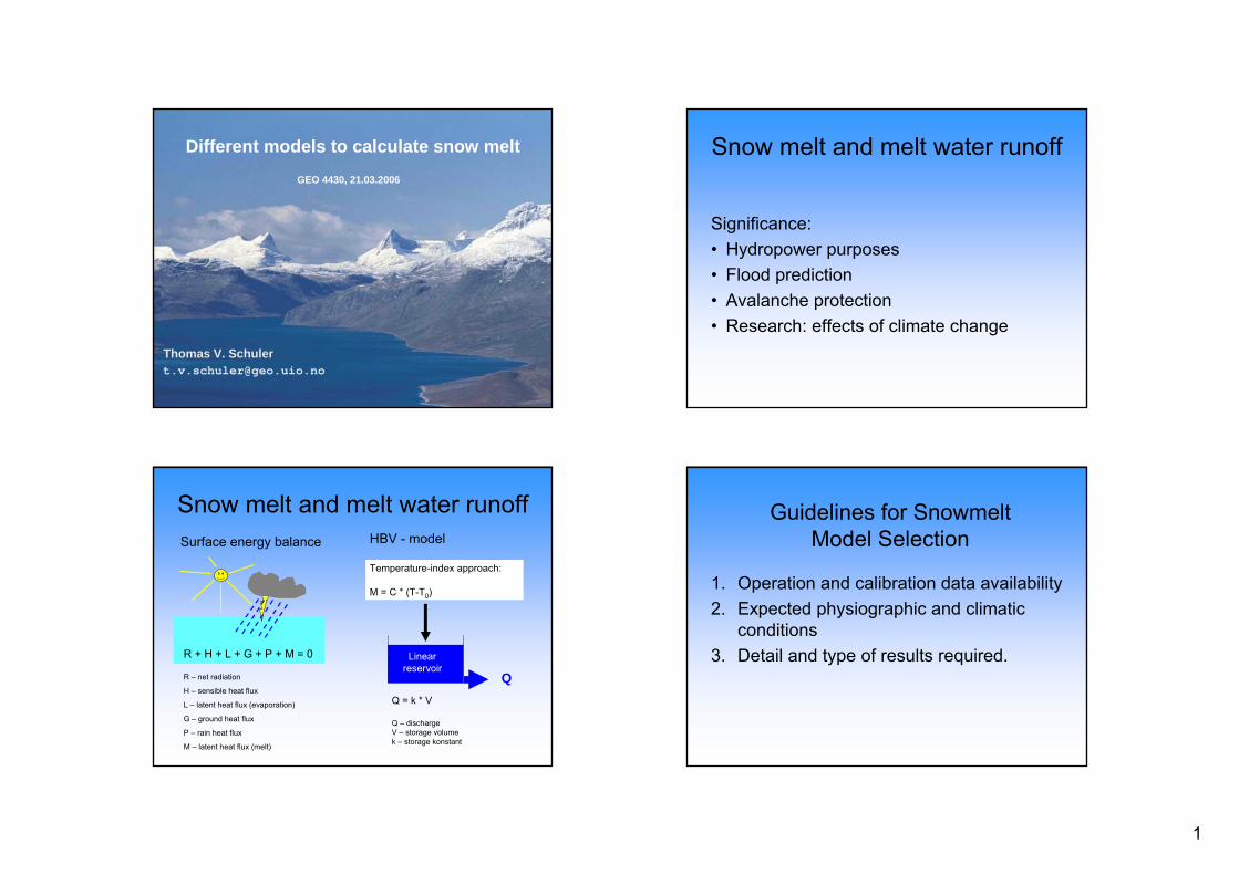
Different models to calculate snow melt
Thomas V. [email protected]
GEO 4430, 21.03.2006
Snow melt and melt water runoff
Significance: • Hydropower purposes• Flood prediction• Avalanche protection• Research: effects of climate change
Snow melt and melt water runoffSurface energy balance
R + H + L + G + P + M = 0
R – net radiation
H – sensible heat flux
L – latent heat flux (evaporation)
G – ground heat flux
P – rain heat flux
M – latent heat flux (melt)
Temperature-index approach:
M = C * (T-T0)
HBV - model
QLinear
reservoir
Q = k * V
Q – dischargeV – storage volumek – storage konstant
Guidelines for Snowmelt Model Selection
1. Operation and calibration data availability2. Expected physiographic and climatic
conditions3. Detail and type of results required.
2
1. Ablation Stakes2. Regression Analysis (linear or multiple)3. Temperature Index Approach 4. Energy Balance Approach
Primary approaches to modeling snowmelt:
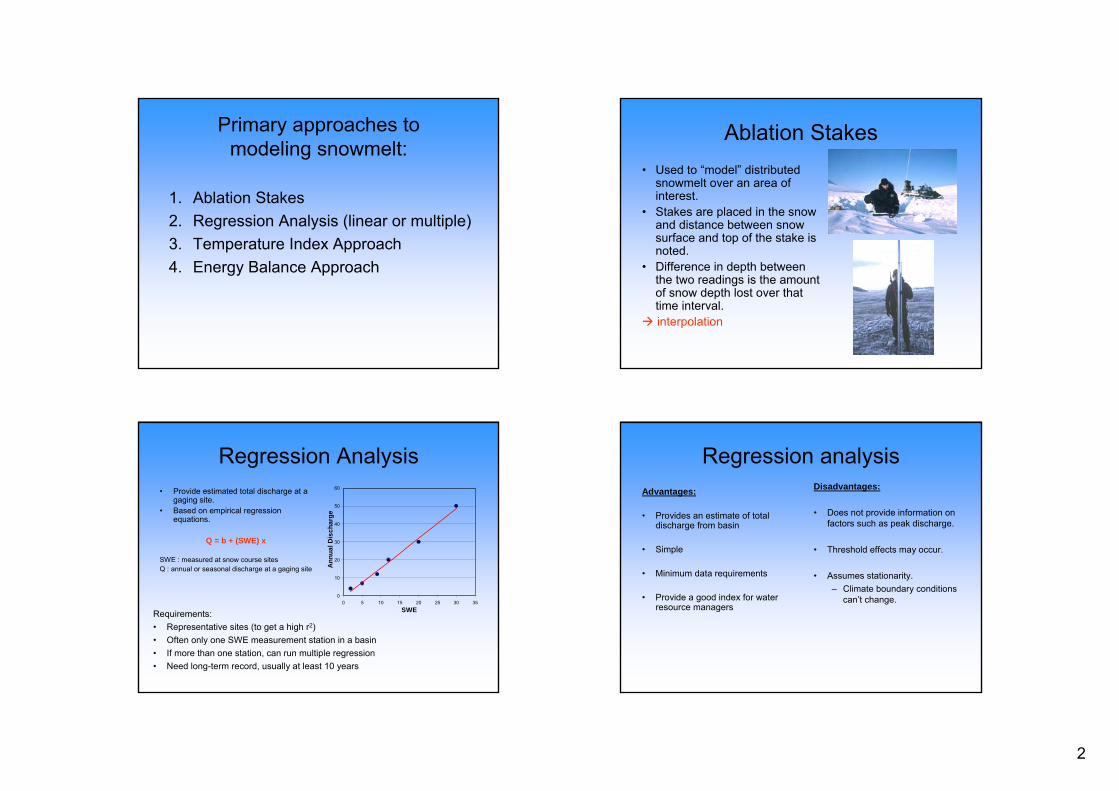
Ablation Stakes• Used to “model” distributed
snowmelt over an area of interest.
• Stakes are placed in the snow and distance between snow surface and top of the stake is noted.
• Difference in depth between the two readings is the amount of snow depth lost over that time interval. interpolation
Regression Analysis• Provide estimated total discharge at a
gaging site.• Based on empirical regression
equations.
Q = b + (SWE) x
SWE : measured at snow course sitesQ : annual or seasonal discharge at a gaging site
0
10
20
30
40
50
60
0 5 10 15 20 25 30 35SWE
Ann
ual D
isch
arge
Requirements:• Representative sites (to get a high r2)• Often only one SWE measurement station in a basin• If more than one station, can run multiple regression• Need long-term record, usually at least 10 years
Regression analysisAdvantages:
• Provides an estimate of total discharge from basin
• Simple
• Minimum data requirements
• Provide a good index for water resource managers
Disadvantages:
• Does not provide information on factors such as peak discharge.
• Threshold effects may occur.
• Assumes stationarity.– Climate boundary conditions
can’t change.
3
Temperature-Index Methods
Based on the concept that changes in air temperature provide an index of snowmelt.T-index approach:
M = C * (T – T0)
Air temperature – commonly measured meteorological variable.– secondary meteorological variable that provides an
integrated measure of heat energy.
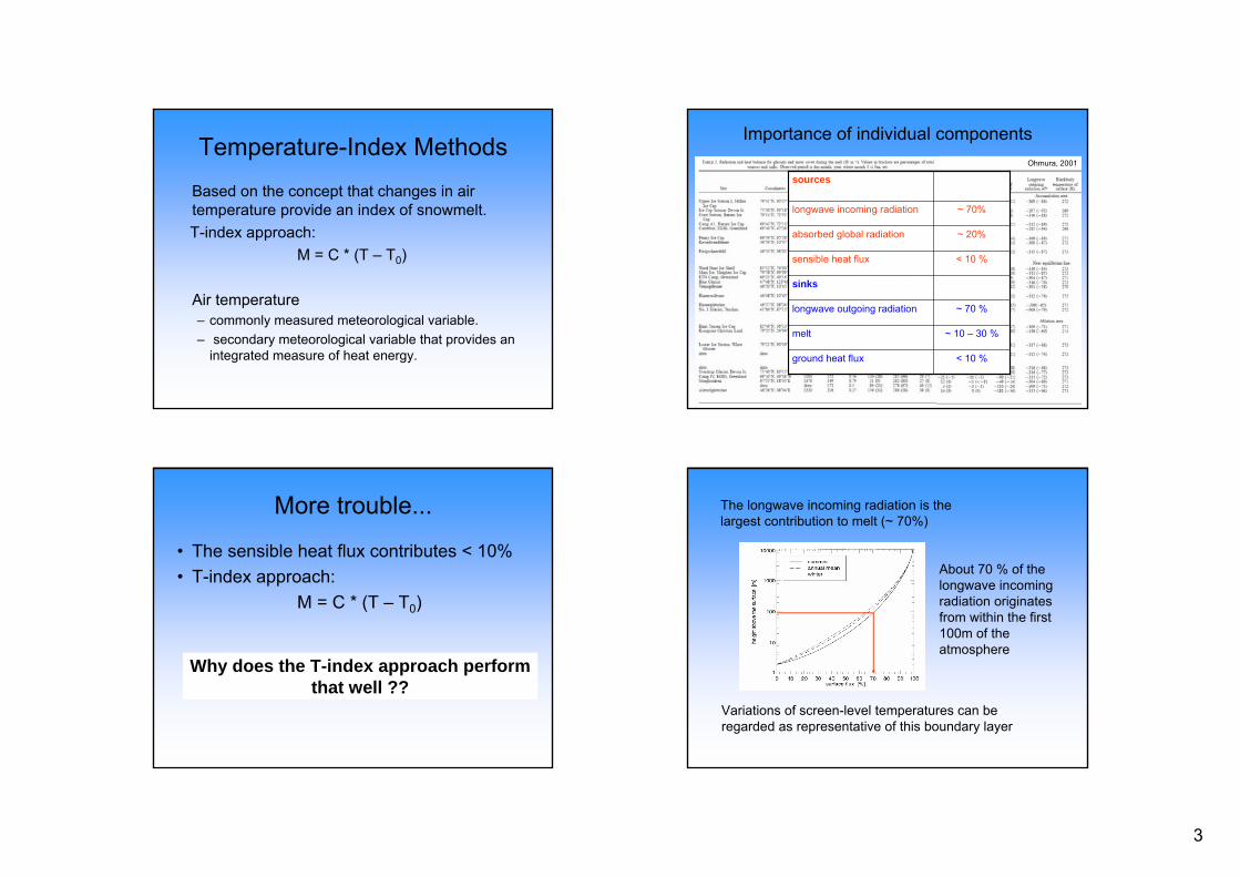
Ohmura, 2001
Importance of individual components
< 10 %ground heat flux
~ 10 – 30 %melt
~ 70 %longwave outgoing radiation
sinks
< 10 %sensible heat flux
~ 20%absorbed global radiation
~ 70%longwave incoming radiation
sources
More trouble...
• The sensible heat flux contributes < 10% • T-index approach:
M = C * (T – T0)
Why does the T-index approach performthat well ??
The longwave incoming radiation is the largest contribution to melt (~ 70%)
About 70 % of the longwave incomingradiation originatesfrom within the first 100m of the atmosphere
Variations of screen-level temperatures can be regarded as representative of this boundary layer
4
Temperature-index models:+ low data demand+ applicable in all scales- trouble with quality control
Photo: Schuler
Energy Balance Models
• Point or spatially distributed
• Run on measured data– contrast to empirical models, which run on only a few measured
parameters and which rely on calibration parameters at the heart of the model.
• Only as good as your measured data and understanding of the system
• Includes some empirism anyway (turbulent exchange…)
• Sacrifice simplicity for complicated measurements and algorithms.
MPGLHR QQQQQQ +++++=0
Energy Balance problems
• Energy Balance model (parameterizations of turbulent exchange)
• Spatial distribution• Precipitation• Snowpack model
(refreezing, metamorphism, water retention)
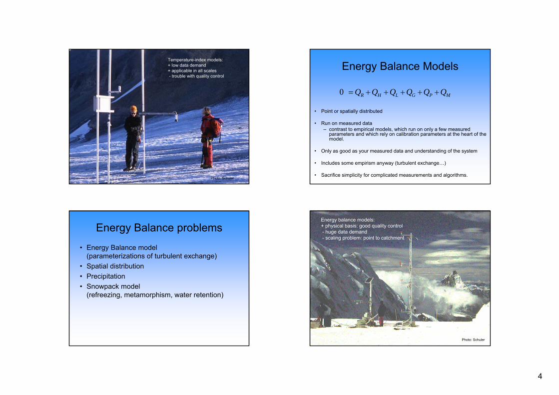
Photo: Schuler
Energy balance models:+ physical basis: good quality control- huge data demand- scaling problem: point to catchment
5
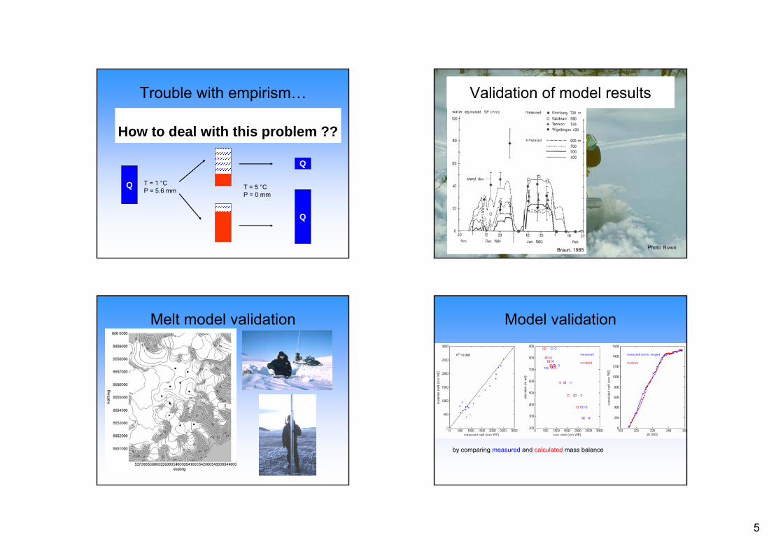
Trouble with empirism…
Q
Given:
T = 1 °CP = 5.6 mm
adjust melt and precipitationparameters to achieveagreement between measuredand calculated Q
Prediction:
T = 5 °CP = 0 mm
Q
Q
How to deal with this problem ??
Validation of model results
Photo: BraunBraun, 1985
Melt model validation Model validation
by comparing measured and calculated mass balance
6
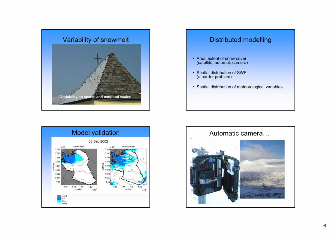
Variability of snowmelt
Variability on spatial and temporal scales
Distributed modelling
• Areal extent of snow cover (satellite, automat. camera)
• Spatial distribution of SWE (a harder problem)
• Spatial distribution of meteorological variables
maskicefirnsnow
Model validation Automatic camera…
7
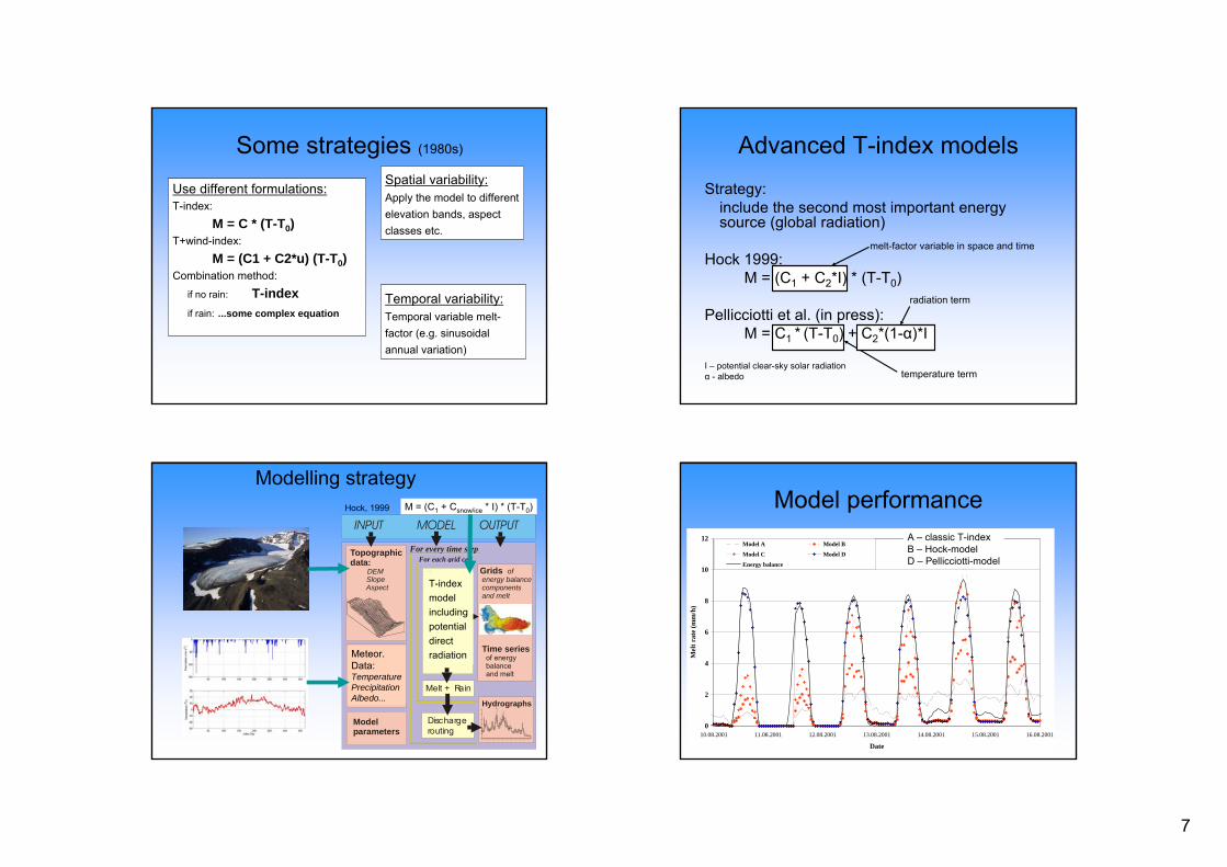
Some strategies (1980s)
Use different formulations:T-index:
M = C * (T-T0)T+wind-index:
M = (C1 + C2*u) (T-T0)Combination method:
if no rain: T-indexif rain: ...some complex equation
Spatial variability:Apply the model to different elevation bands, aspectclasses etc.
Temporal variability:Temporal variable melt-factor (e.g. sinusoidalannual variation)
temperature term
melt-factor variable in space and time
radiation term
Advanced T-index models
Strategy:include the second most important energy source (global radiation)
Hock 1999:M = (C1 + C2*I) * (T-T0)
Pellicciotti et al. (in press):M = C1 * (T-T0) + C2*(1-α)*I
I – potential clear-sky solar radiationα - albedo
Modelling strategy
Topographicdata: DEM Slope Aspect
Meteor. Data: Temp Humidity Wind speed Global radiation ...
Modelparameters
Grids of energy balance components and melt
Discharge routing
Melt + Rain
Energy balancemodel
Temp indexmodel: - degree day - including pot direct rad
Hydrographs
Time series of energy balance and melt
For every time stepFor each grid cell
or
Meteor. Data:TemperaturePrecipitationAlbedo...
T-indexmodelincludingpotentialdirectradiation
Hock, 1999 M = (C1 + Csnow/ice * I) * (T-T0)
0
2
4
6
8
10
12
10.08.2001 11.08.2001 12.08.2001 13.08.2001 14.08.2001 15.08.2001 16.08.2001
Date
Mel
t rat
e (m
m/h
)
Model A Model B
Model C Model D
Energy balance
Model performanceA – classic T-indexB – Hock-modelD – Pellicciotti-model
8
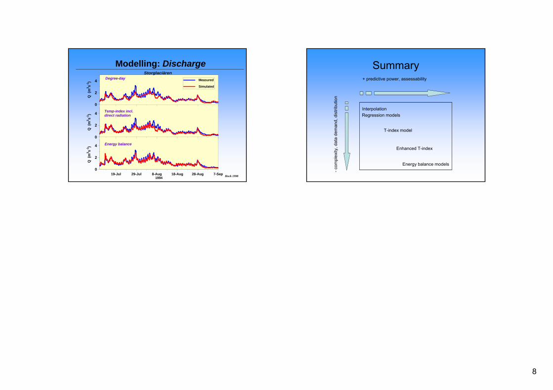
Modelling: Discharge
Hock 199819-Jul 29-Jul 8-Aug 18-Aug 28-Aug 7-Sep1994
0
2
4
Q (
m3 s-1
)
0
2
4
Q (
m3 s-1
)
0
2
4
Q (
m3 s-1
)
StorglaciärenDegree-day
Temp-index incl.direct radiation
Energy balance
Measured
Simulated
Summary+ predictive power, assessability
-com
plex
ity, d
ata
dem
and,
dis
tribu
tion
Energy balance models
InterpolationRegression models
T-index model
Enhanced T-index
Top Related