Sketching Interfaces for 2D Animation of Simple Objects

Jimmy Ho Department of Computer Science

Brown University

Submitted in partial fulfillment of the requirments for the Degree of Master of Sciences in the Department Computer Science at Brown University.

hn Hughes, Project Advisor) Date

1

Sketching Interfaces for 2D Animation of Simple Objects

Jimmy Ho'

Computer Science Department, Brown University, Providence, RI 02912-1910

Abstract

This report describes efforts to apply sketching interfaces to animation. We deal with the problem of sketching 2-D mo­tion paths for objects to produce animations for applications like Microsoft PowerPoint , Macromedia Flash or Director. We worked on the core problem of editing a sketched mo­tion curve, using the approach of blending newly sketched motion paths with older paths to allow for successive refine­ments of an animation. We describe various methods used to edit motion curves and their results.

1 Introduction

1.1 Background

This paper deals with building a gestural interface for the two-dimensional animation of simple objects. There are many applications that use 2-D.animations, such as Macro­media's Flash, Director and Shockwave applications, or even Microsoft's PowerPoint presentation software, which deliver traditional 2-D graphic art with movement and sound. This sort of animation can also be seen in fast paced commer­cials that use moving textual messages to make their point. Thus, in our context, "simple objects" can be imagined as pictures, text or simple shapes (as opposed to animating Bugs Bunny or some other articulated figure). Animation of these objects include both linear and angular motion, as well as having these objects fading in/out, changing size, morph­ing into other objects, or even physically-based animation, all within a 2-D space.

There are already methods for producing animations, includ­ing key-framing, physically-based animation, and just man­ually specifying all the relevant functions (x(t), Yet), (J(t), shape(t), transparency(t), etc.). The last approach is obvi­ously tedious. Key-framing, while not as tedious, especially in 2-D, can still be painstakingly slow. 1 Physically-based techniques work well only for things that seem to simulate a physical process, such as a bouncing ball. Even then, a user could much more quickly sketch the motion with a mouse or pen device and achieve a reasonable imitation, which is suf­ficient given the types of applications that we are looking at (i.e., PowerPoint or Flash animations with objects moving in an abstract space where people don't expect completely realistic physics). What we need then is an intuitive way to sketch animations without a lot of excess point-and-click, typing and arithmetic.

A sketching, or gestural, interface is characterized by "ges­tures," which are hand-drawn marks that issue a command to the computer. Gestures are different from buttons and

·jkh@cs.brown.edu 1 "Painstakingly slow:" Taking more than 30 seconds to create

and fine tune, say, a winding, three-inch-long, S-shaped path with a pause at the first bend and a little wiggle at the end

) (a) (b) (c)

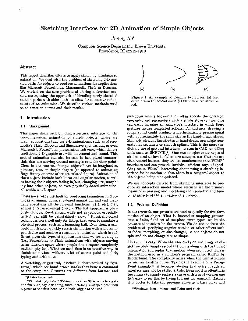
Figure 1 An example of blending two curves. (a) first curve drawn (b) second curve (c) blended curve shown in red.

pull-down menus because they often specify the operator, operands, and parameters with a single stoke or two. One can easily imagine an animator's interface in which these gestures invoke templated actions. For instance, drawing a rough spiral could produce a mathematically precise spiral with approximately the same size as the hand-drawn stroke. Similarly, straight line strokes or hand-drawn arcs might gen­erate line segments or smooth splines. This is the more tra­ditional use of gestural interfaces, as seen in CAD modelling tools such as SKETCH[8]. One can imagine other types of strokes used to invoke fades, size changes, etc. Gestures are often touted because they are less cumbersome than WIMp2

interfaces and can provide intuitive, efficient ways of speci­fying tasks. What's interesting about using a sketching in­terface for animation is that there is a temporal aspect to the objects being manipulated.

We use concepts derived from sketching interfaces to pro­duce an interaction model where gestures are the primary means of expressing and modifying the geometric and tem­poral aspects of the animation of an object.

1.2 Problem Definition

In our research, our gestures are used to specify the free-form motion of an object. That is, instead of mapping gestures onto a finite, fixed set of template curve types, we let the gestures themselves be the curves. We do not address the problem of specifying angular motion or other effects such as fades, morphing, or size-changes, so our objects do not spin and do not change size or shape.

This sounds easy: When the user clicks on and drags an ob­ject, we could simply record the points along with the timing information and replay that motion when prompted. This is the method used in a children's program called KidPix by Broderbund. The complexity arises when the user attempts to edit an existing curve. Taking the example of a Power­Point animation, it becomes obvious that users of such an interface may not be skilled artists. Even so, it is oftentimes too clumsy to simply replace a curve with a newly-drawn one (it's easy to see this by trying this out for yourself). Rather, it is better to take the previous curve as a base curve and

2Windows, Icons, Menus and Point-and-click

modify it by drawing another curve. This involves blending two curves in an intuitive way (see Figure 1). Unfortunately, "editing" a curve not only involves editing the shape of the curve, but the timing information as well: a user may like the shape just fine, but might want some part of the ani­mation to move at a different speed, or to elongate a pause, etc. The obvious approach (and the one that we use) is to just have the user redraw the curve at the desired speed. Obviously, the user cannot and should not have to redraw the prior curve exactly and thus, it is up to the computer to figure out how to relate the two curves so that the timing in­formation from the second curve is appropriately overlayed onto the first curve. This process is complicated by the fact that the source for the curves is a collection of discrete sam­ples with non-uniform sampling rates and unevenly-spaced points.

Therefore, we let a user specify a free-form 2-D motion path by successively refining it. This is done by blending new curves with previously drawn curves, which requires that we establish a good point-to-point correspondence between pairs of curves. That is, given two discrete curves y(r) and Q(r), we want to find a curve ~(r) which gives an intuitive blend of y(r) and Q(r). r is an arbitrary parameter. In the course of describing different algorithms, we will parameter­ize the curve using path length, time, and point index. This ability to match curve points allows us to do some general tasks that an algorithm can perform when the user draws two successive motion curves by clicking and dragging the same object twice:

1. Blend the shapes of both curves to produce a new curve, but keep the timing information of the old curve.

2. Keep the old shape but use timing information of the new curve.

3. Both of the above.

In the course of our research, we focused mainly on case 1, since case 2 can be implemented once a correspondence is established, which is a necessary result of solving the shape blending problem. We designed and implemented various methods, with varying degrees of success. The discussion of these methods constitute the rest of the paper.

1.3 Related Work

Trying to establish a point-to-point correspondence between two discrete curves has been a problem in many fields. Re­search in gestural interfaces contribute to the solution in the form of gesture-recognizers, However recent research in gesture recognizers seem focused on extracting specific inter­esting features that are not general enough to use to match a pair of curves whose shapes are arbitrary but similar to one another[6], while others use "training sets," which are not applicable here since the user produces the two curves that require matching in real time[3J[4].

Handwriting recognition researchers have long sought ways to match hand-written letters and words to a finite alphabet. The difference between our research and that of handwriting recognition is that there is no fixed set of curves or training set to take advantage of (via preprocessing, using Hidden Markov Models, etc.).

One other method is elastic matching. This usually involes treating one curve as a metal wire that is stretched and

bent to match the other curve. Choosing some sort of least energy solution, one finds a correspondence along with a set of stretches and bends to interpolate a blend. Uses include 2-D morphing[2]. While this method has its merits, we did not investigate these algorithms in depth.

1.4 Notation and Terminology

When a user draws a stroke that specifies a free-form ani­mation curve, we will refer to that as a "curve" or "path." The naming conventions in the source code tend to use these conventions as well. Unless otherwise noted, distances are in pixels and units of time are in milliseconds.

To establish better correspondence between the concepts in this report and the code written to implement it, ref­erences to Java packages and classes are represented by classname, packagename, or packagename.classname. For instance, PathEditFactory or pathedit .PathEditFactory.

2 Overall Methodology and Algorithm Structure

Similar to techniques used in gesture and handwriting recog­nition, we have preprocessing phases for the strokes in order to weed out noise and irrelevant details. Then we apply some algorithm which establishes a correspondence. Once a cor­respondence if found, it is a simple matter to interpolate the new curve. Thus, after two successive motion paths are drawn, the following steps occur:

Establish Interpolate Correspondence New Curve

In the Pre-Filter step, we apply a special filter to both y(r) and Q(r) that deletes points that are spaced too closely together (usually less than a few pixels) and adds points where they are spaced too far apart. Points that are spaced only a few pixels apart are often too noisy and reduce the efficiency of our algorithms. Also, during animation, such closely spaced points often slow down the animation, pro­ducing an unfaithful reproduction of the user's stroke. Be­cause we often interpolate the two motion paths by using all the points of y(r) but not necessarily all the points of Q(r) (to retain the original timing information), it is essen­tial that we start with lots of points, so that the resultant blended curves are not too coarse. This is the rationale for adding points where they are spaced too far apart. For more details, see filter. FilterPreFilter.

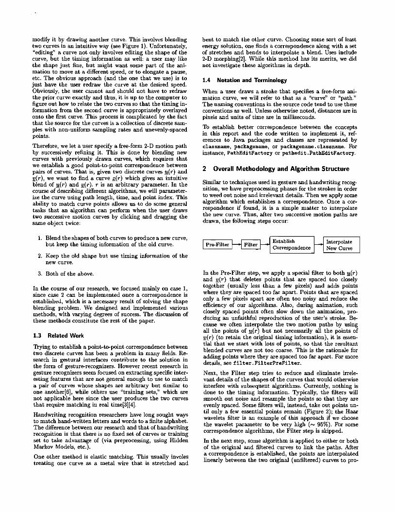
Next, the Filter step tries to reduce and eliminate irrele­vant details of the shapes of the curves that would otherwise interfere with subsequent algorithms. Currently, nothing is done to the timing information. Typically, the filters will smooth out noise and resample the points so that they are evenly spaced. Some filters will, instead, take out points un­til only a few essential points remain (Figure 2); the Haar wavelets filter is an example of this approach if we choose the wavelet parameter to be very high ('" 95%). For some correspondence algorithms, the Filter step is skipped.

In the next step, some algorithm is applied to either or both of the original and filtered curves to link the paths. After a correspondence is established, the points are interpolated linearly between the two original (unfiltered) curves to pro­

(a) (b)

Figure 2 (a) A smoothing filter that resamples the points evenly and more closely spaced. (b) A Haar wavelet filter that extracts out only the important features by combin­ing/eliminating the other points.

duce a final result.

The Pre-Filter is fixed and does not change. Different al­gorithms in the Filter step can be combined with different correspondence algorithms to achieve different results. The actual blending of the curves, once a correspondence has been established, is straightforward. Most of this paper deals with the "Establish Correspondence" step.

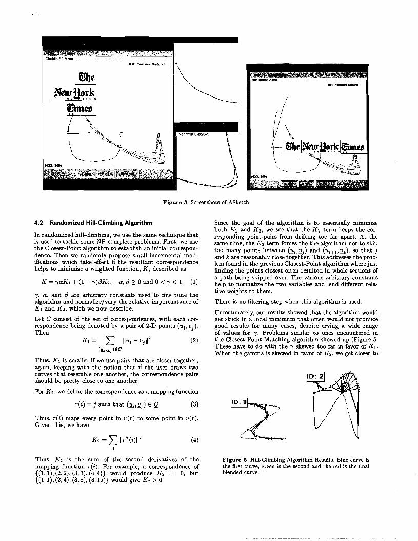
3 ASketch

In the course of doing our research, we have developed an application to implement and test our ideas. The project, named ASketch (for Animation Sketch), was conceived and engineered during the 1999-2000 school year. ASketch con­tains the implementation of the algorithms discussed in this report. (See Figure 3)

The application has a main window with a "Sketching Area." A user can add, delete, duplicate and move widgets, as well as specify motion curves by dragging these widgets around. Animations can be played by clicking a single button. The objects' animation curves can be edited via different algo­rithms. There is unlimited undo and redo, and the we use a marking-menu interface. There are also separate windows to view results from filters and feature detection algorithms.

More details of how the application works can be found in the Users' Manual and Programmers' Reference (if they get written).

4 Early Algorithms

In the course of our research, we tried different algorithms. We begin by detailing our early efforts, most of which failed, and finish with our more successful algorithms.

All the algorithms listed below describe the method by which a correspondence was found between two curves based on their geometric shape. We do not discuss how to actually in­terpolate between the curves because in all cases the method is straightforward.

4.1 Closest Point Matching Algorithm

At the outset, it seemed reasonable that since the user is likely to draw the two paths roughly alike, a point in one curve would be the closest point to its corresponding point in the other. Therefore, our first algorithm matched each point on one curve to the closest point on the other curve.

K.I~~~ Sketching Area

SP: Blend Neive C~e&t

(a) (b)

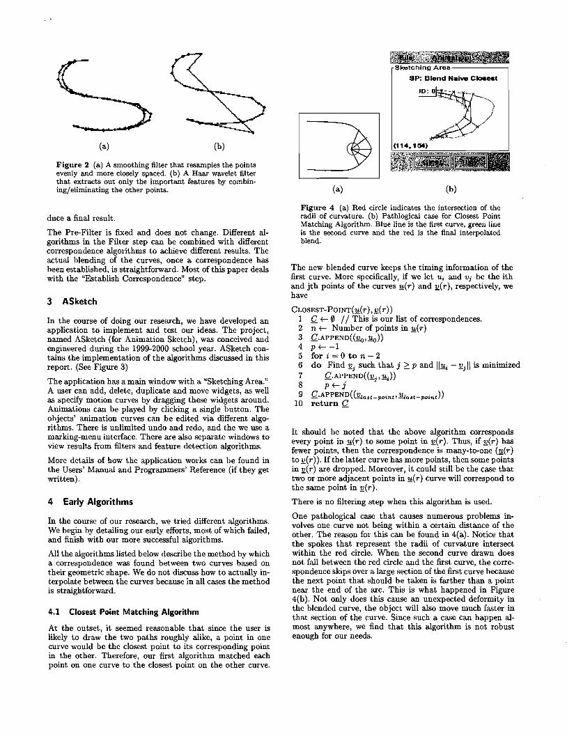
Figure 4 (a) Red circle indicates the intersection of the radii of curvature. (b) Pathlogical case for Closest Point Matching Algorithm. Blue line is the first curve, green line is the second curve and the red is the final interpolated blend.

The new blended curve keeps the timing information of the first curve. More specifically, if we let Ui and Vj be the ith and jth points of the curves 1!(r) and ~(r), respectively, we have

CLOSEST-POINT(1!(r), ~(r» 1 Q t- 0 / / This is our list of correspondences. 2 nt-Number of points in 1!(r) 3 Q.APPENo«11o, Yo» 4 p t--l 5 for i == 0 to n ­ 2 6 do Find ~j such that j ~ p and II1!i - ~j II is minimized 7 Q.APPENO«~j,1!i» 8 pt-j 9

10 Q.APPENO( (~a8t-point' 1!la8t-point» return Q

It should be noted that the above algorithm corresponds every point in 1!(r) to some point in ~(r). Thus, if ~(r) has fewer points, then the correspondence is many-to-one (1!(r) to ~(r». If the latter curve has more points, then some points in ~(r) are dropped. Moreover, it could still be the case that two or more adjacent points in g( r) curve will correspond to the same point in ~(r).

There is no filtering step when this algorithm is used.

One pathological case that causes numerous problems in­volves one curve not being within a certain distance of the other. The reason for this can be found in 4(a). Notice that the spokes that represent the radii of curvature intersect within the red circle. When the second curve drawn does not fall between the red circle and the first curve, the corre­spondence skips over a large section of the first curve because the next point that should be taken is farther than a point near the end of the arc. This is what happened in Figure 4(b). Not only does this cause an unexpected deformity in the blended curve, the object will also move much faster in that section of the curve. Since such a case can happen al­most anywhere, we find that this algorithm is not robust enough for our needs.

8P: Feeture MMgh 1

·.--~_. ~._-_.._----­ ~~-'--'-~i

I

I

m1)el Ne~Dt?r~J

Iimt~..

Figure 3 Screenshots of ASketch

4.2 Randomized Hill-Climbing Algorithm

In randomized hill-climbing, we use the same technique that is used to tackle some NP-complete problems. First, we use the Closest-Point algorithm to establish an initial correspon­dence. Then we randomly propose small incremental mod­ifications which take effect if the resultant correspondence helps to minimize a weighted function, K, described as

K = ,aKI + (1 - ,)/3K2, a, /3 ~ 0 and 0 < , < 1. (1)

" a, and /3 are arbitrary constants used to fine tune the algorithm and normalize/vary the relative importantance of Kl and K 2 , which we now describe.

Let C consist of the set of correspondences, with each cor­respondence being denoted by a pair of 2-D points (11<;,1l.j)' Then

tc, = L 1111<; - Qj l12 (2) (!!.;.1!.j)EC

Thus, K 1 is smaller if we use pairs that are closer together, again, keeping with the notion that if the user draws two curves that resemble one another, the correspondence pairs should be pretty close to one another.

For K2, we define the correspondence as a mapping function

r(i) = j such that (11<;, Qj) E Q (3)

Thus, r(i) maps every point in 11«r) to some point in Q(r). Given this, we have

(4)

Since the goal of the algorithm is to essentially minimize both K 1 and K 2, we see that the K 1 term keeps the cor­responding point-pairs from drifting too far apart. At the same time, the K 2 term forces the the algorithm not to skip too many points between (1!<;, Qj) and (1!<; l' Qk)' so that j and k are reasonably close togetlier. This a~dresses the prob­lem found in the previous Closest-Point algorithm where just finding the points closest often resulted in whole sections of a path being skipped over. The various arbitrary constants help to normalize the two variables and lend different rela­tive weights to them.

There is no filtering step when this algorithm is used.

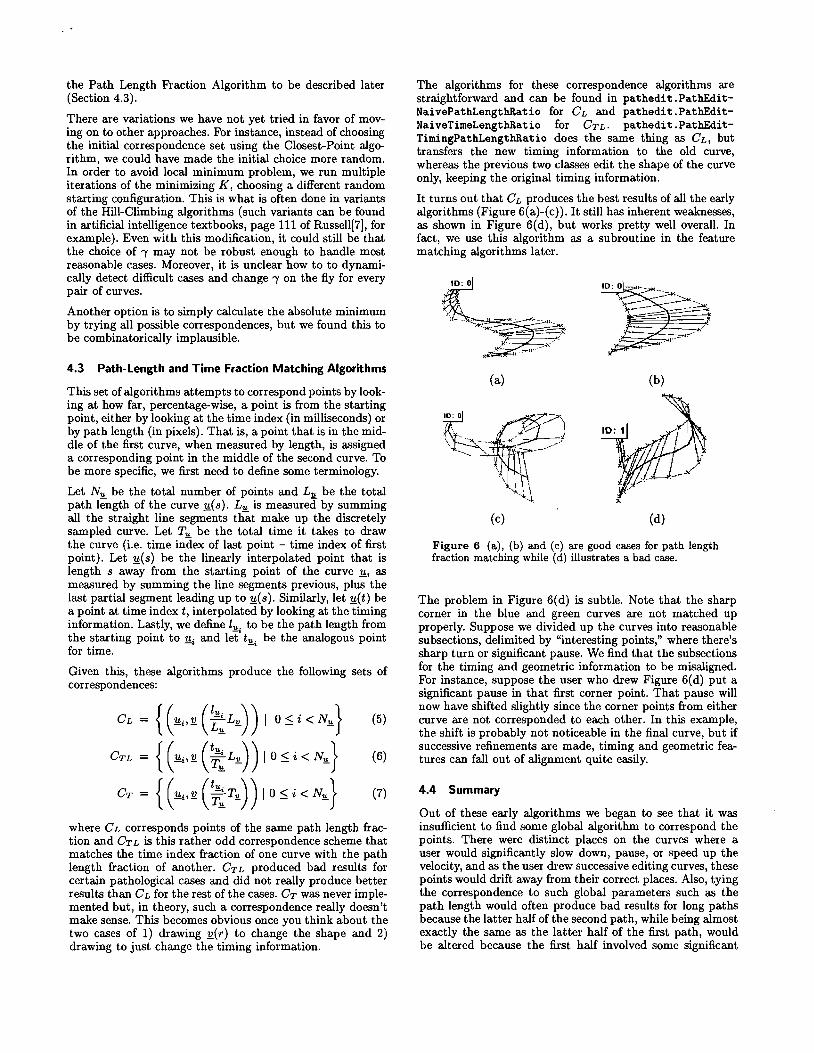
Unfortunately, our results showed that the algorithm would get stuck in a local minimum that often would not produce good results for many cases, despite trying a wide range of values for ,. Problems similar to ones encountered in the Closest Point Matching algorithm showed up (Figure 5. These have to do with the, skewed too far in favor of K 1.

When the gamma is skewed in favor of K2, we get closer to

Thus, K2 is the sum of the second derivatives of the Figure 5 Hill-Climbing Algorithm Results. Blue curve is mapping function r(i). For example, a correspondence of the first curve, green is the second and the red is the final {(I, 1), (2, 2), (3,3), (4, 4)} would produce K2 = 0, but blended curve. {(I, 1), (2,4), (3,8), (3, 15)} would give K2 > O.

the Path Length Fraction Algorithm to be described later (Section 4.3).

There are variations we have not yet tried in favor of mov­ing on to other approaches. For instance, instead of choosing the initial correspondence set using the Closest-Point algo­rithm, we could have made the initial choice more random. In order to avoid local minimum problem, we run multiple iterations of the minimizing K, choosing a different random starting configuration. This is what is often done in variants of the Hill-Climbing algorithms (such variants can be found in artificial intelligence textbooks, page 111 of Russell[7], for example). Even with this modification, it could still be that the choice of "y may not be robust enough to handle most reasonable cases. Moreover, it is unclear how to to dynami­cally detect difficult cases and change "y on the fly for every pair of curves.

Another option is to simply calculate the absolute minimum by trying all possible correspondences, but we found this to be combinatorically implausible.

4.3 Path-Length and Time Fraction Matching Algorithms

This set of algorithms attempts to correspond points by look­ing at how far, percentage-wise, a point is from the starting point, either by looking at the time index (in milliseconds) or by path length (in pixels). That is, a point that is in the mid­dle of the first curve, when measured by length, is assigned a corresponding point in the middle of the second curve. To be more specific, we first need to define some terminology.

Let N; be the total number of points and Lv. be the total path length of the curve y.(s). L~ is measured by summing all the straight line segments that make up the discretely sampled curve. Let Tv. be the total time it takes to draw the curve (i.e. time index of last point - time index of first point). Let y'(s) be the linearly interpolated point that is length s away from the starting point of the curve y., as measured by summing the line segments previous, plus the last partial segment leading up to y'(s). Similarly, let y.(t) be a point at time index t, interpolated by looking at the timing information. Lastly, we define l«. to be the path length from the starting point to y.; and let t~ be the analogous point for time.

Given this, these algorithms produce the following sets of correspondences:

CL = {(y.;, Q (?~ L~) ) I 0 s i < N~} (5)

CTL = {(y.;, Q (~ L~) ) I 0 s i < N~} (6)

CT = { (y.;,Q (~ T~) ) I 0 s i < N~} (7)

where CL corresponds points of the same path length frac­tion and CTL is this rather odd correspondence scheme that matches the time index fraction of one curve with the path length fraction of another. CTL produced bad results for certain pathological cases and did not really produce better results than CL for the rest of the cases. CT was never imple­mented but, in theory, such a correspondence really doesn't make sense. This becomes obvious once you think about the two cases of 1) drawing Q(r) to change the shape and 2) drawing to just change the timing information.

The algorithms for these correspondence algorithms are straightforward and can be found in pathedit.PathEdit­NaivePathLengthRatio for CL and pathedit.PathEdit­NaiveTimeLengthRatio for CTL. pathedit.PathEdit­TimingPathLengthRatio does the same thing as CL, but transfers the new timing information to the old curve, whereas the previous two classes edit the shape of the curve only, keeping the original timing information.

It turns out that CL produces the best results of all the early algorithms (Figure 6(a)-(c». It still has inherent weaknesses, as shown in Figure 6(d), but works pretty well overall. In fact, we use this algorithm as a subroutine in the feature matching algorithms later.

(a) (b)

(c) (d)

Figure 6 (a), (b) and (c) are good cases for path length fraction matching while (d) illustrates a bad case.

The problem in Figure 6(d) is subtle. Note that the sharp corner in the blue and green curves are not matched up properly. Suppose we divided up the curves into reasonable subsections, delimited by "interesting points," where there's sharp turn or significant pause. We find that the subsections for the timing and geometric information to be misaligned. For instance, suppose the user who drew Figure 6(d) put a significant pause in that first corner point. That pause will now have shifted slightly since the corner points from either curve are not corresponded to each other. In this example, the shift is probably not noticeable in the final curve, but if successive refinements are made, timing and geometric fea­tures can fallout of alignment quite easily.

4.4 Summary

Out of these early algorithms we began to see that it was insufficient to find some global algorithm to correspond the points. There were distinct places on the curves where a user would significantly slow down, pause, or speed up the velocity, and as the user drew successive editing curves, these points would drift away from their correct places. Also, tying the correspondence to such global parameters such as the path length would often produce bad results for long paths because the latter half of the second path, while being almost exactly the same as the latter half of the first path, would be altered because the first half involved some significant

5

differences. It is with these issues in mind that we move on to feature matching algorithms.

Later Algorithms

In these later algorithms, we focused more on subdividing curves into more manageable pieces, which resulted in better correspondence algorithms.

These algorithms utilize feature matching and feature de­tection techniques to correspond points. Thus, we attempt to subdivide a motion curve into pieces and find correspon­dences for each piece. In general, the correspondence algo­rithm attempts to detect the "interesting" features for both 1f.(r) and !l(r). It then tries to match up the features from both curves, thus setting up a correspondence between the features. After this step, the curves will have corresponding subsections for which we use a simple Path Length Fraction correspondence algorithm (GL or GT) to link. Thus, the gen­eral flow of execution now looks like

~ - - - - - - - - - - "Esta.blisn-Ciii'respiiiiaence - - - - - - - - - - -; , ,, ,, , , , , ,,,

At the Filter step, we apply a variety of filters, described below. The feature detection algorithms then use curvature data that is derived from the filtered curve to find features that produce curvature extrema. The curvature data consists getting the direction change as we move from one line segment to another along the discretized motion path (Figure 7). Curvature extrema are detected by examining a plot of the curvature data and noticing those parts of the plot that deviate beyond a calculated threshold value from zero.

B C

A

Figure 7 A, B and C are consecutive points on somecurve. The curvature info for point B is () (radians).

When establishing a point-to-point correspondence, we cor­respond the points in the original curves (not the filtered curves). Thus, each feature found in Feature Detection has a time index that links back to a point on the original curve.

SP: Feature Match 1

(a)

(b) dalacurvalure4

-0.2 .

-0.4 .

-0.6 .

-0.8 .

-1 L-_--'-_---'-__"--_-'-_---J o 20 40 80 80 100

(c)

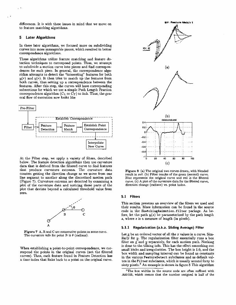
Figure 8 (a) The original two curves drawn, with blended result in red. (b) Filter results of the green (second) curve. Blue represents the original curve and red is the filtered curve. (c) A plot of the curvature data for the filtered curve, direction change (radians) vs. point index.

5.1 Filters

This section presents an overview of the filters we used and their results. More information can be found in the source code in the SketchingAnimation.filter package. As be­fore, let the path 1f.(s) be parameterized by the path length s, where s is a measure of length (in pixels).

5.1.1 Regularization [a.k.a. Sliding Average) Filter

Let :!<. be an ordered vector of all the x values in a curve. Sim­ilarly for y. The regularization filter essentially runs a box filter on £ and y separately, for each motion path. Nothing is done to the timing info. This has the effect smoothing out small kinks and irregularities. The box height is 1.0, and the box width and sampling interval can be found as constants in the various FeatureDetect subclasses and as default val­ues in the Filter subclasses, which is usually around forty to sixty pixels.3 An example is shown in figure 8 This algorithm

3The box widths in the source code are often suffixed with ...RADIUS, which means that the number assigned is half of the

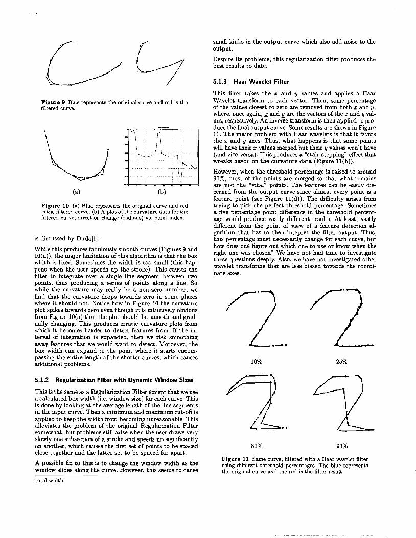
Figure 9 Blue represents the original curve and red is the filtered curve.

(a) (b)

Figure 10 (a) Blue represents the original curve and red is the filtered curve. (b) A plot of the curvature data for the filtered curve, direction change (radians) vs, point index.

is discussed by Duda[l].

While this produces fabulously smooth curves (Figures 9 and 10(a)), the major limitation of this algorithm is that the box width is fixed. Sometimes the width is too small (this hap­pens when the user speeds up the stroke). This causes the filter to integrate over a single line segment between two points, thus producing a series of points along a line. So while the curvature may really be a non-zero number, we find that the curvature drops towards zero in some places where it should not. Notice how in Figure 10 the curvature plot spikes towards zero even though it is intuitively obvious from Figure 10(a) that the plot should be smooth and grad­ually changing. This produces erratic curvature plots from which it becomes harder to detect features from. If the in­terval of integration is expanded, then we risk smoothing away features that we would want to detect. Moroever, the box width can expand to the point where it starts encom­passing the entire length of the shorter curves, which causes additional problems.

5.1.2 Regularization Filter with Dynamic Window Sizes

This is the same as a Regularization Filter except that we use a calculated box width (i.e. window size) for each curve. This is done by looking at the average length of the line segments in the input curve. Then a minimum and maximum cut-off is applied to keep the width from becoming unreasonable. This alleviates the problem of the original Regularization Filter somewhat, but problems still arise when the user draws very slowly one subsection of a stroke and speeds up significantly on another, which causes the first set of points to be spaced close together and the latter set to be spaced far apart.

A possible fix to this is to change the window width as the window slides along the curve. However, this seems to cause

total width

small kinks in the output curve which also add noise to the output.

Despite its problems, this regularization filter produces the best results to date.

5.1.3 Haar Wavelet Filter

This filter takes the x and y values and applies a Haar Wavelet transform to each vector. Then, some percentage of the values closest to zero are removed from both 2<. and y, where, once again, 2<. and y are the vectors of the x and y var­ues, respectively. An inverse transform is then applied to pro­duce the final output curve. Some results are shown in Figure 11. The major problem with Haar wavelets is that it favors the x and y axes. Thus, what happens is that some points will have their x values merged but their y values won't have (and vice-versa). This produces a "stair-stepping" effect that wreaks havoc on the curvature data (Figure l1(b)).

However, when the threshold percentage is raised to around 90%, most of the points are merged so that what remains are just the "vital" points. The features can be easily dis­cerned from the output curve since almost every point is a feature point (see Figure l1(d)). The difficulty arises from trying to pick the perfect threshold percentage. Sometimes a five percentage point difference in the threshold percent­age would produce vastly different results. At least, vastly different from the point of view of a feature detection al­gorithm that has to then intepret the filter output. Thus, this percentage must necessarily change for each curve, but how does one figure out which one to use or know when the right one was chosen? We have not had time to investigate these questions deeply. Also, we have not investigated other wavelet transforms that are less biased towards the coordi­nate axes.

10% 25%

80% 93%

Figure 11 Same curve, filtered with a Haar wavelet filter using different threshold percentages. The blue represents the original curve and the red is the filter result.

_,_.L--',-----=---!,--i:-----=--!

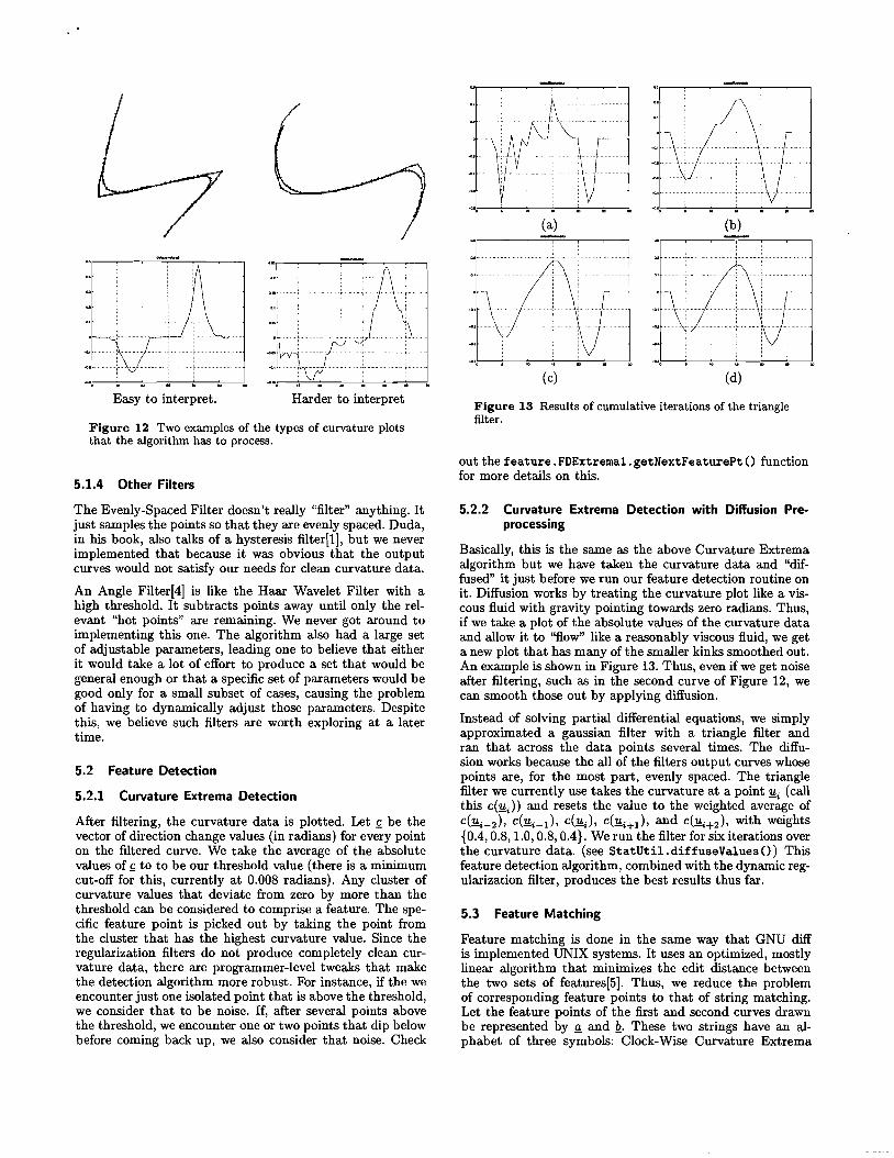
Easy to interpret. Harder to interpret

Figure 12 Two examples of the types of curvature plots that the algorithm has to process.

5.1.4 Other Filters

The Evenly-Spaced Filter doesn't really "filter" anything. It just samples the points so that they are evenly spaced. Duda, in his book, also talks of a hysteresis filter[l], but we never implemented that because it was obvious that the output curves would not satisfy our needs for clean curvature data.

An Angle Filter[4] is like the Haar Wavelet Filter with a high threshold. It subtracts points away until only the rel­evant "hot points" are remaining. We never got around to implementing this one. The algorithm also had a large set of adjustable parameters, leading one to believe that either it would take a lot of effort to produce a set that would be general enough or that a specific set of parameters would be good only for a small subset of cases, causing the problem of having to dynamically adjust those parameters. Despite this, we believe such filters are worth exploring at a later time.

5.2 Feature Detection

5.2.1 Curvature Extrema Detection

After filtering, the curvature data is plotted. Let 5< be the vector of direction change values (in radians) for every point on the filtered curve. We take the average of the absolute values of 5< to to be our threshold value (there is a minimum cut-off for this, currently at 0.008 radians). Any cluster of curvature values that deviate from zero by more than the threshold can be considered to comprise a feature. The spe­cific feature point is picked out by taking the point from the cluster that has the highest curvature value. Since the regularization filters do not produce completely clean cur­vature data, there are programmer-level tweaks that make the detection algorithm more robust. For instance, if the we encounter just one isolated point that is above the threshold, we consider that to be noise. If, after several points above the threshold, we encounter one or two points that dip below before coming back up, we also consider that noise. Check

(a) (b)

(c) (d)

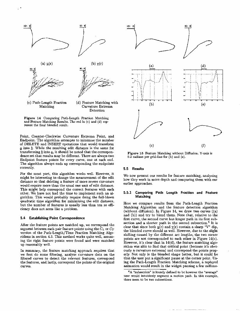
Figure 13 Results of cumulative iterations of the triangle filter.

out the feature. FDExtremal. getNextFeaturePt 0 function for more details on this.

5.2.2 Curvature Extrema Detection with Diffusion Pre­processing

Basically, this is the same as the above Curvature Extrema algorithm but we have taken the curvature data and "dif­fused" it just before we run our feature detection routine on it. Diffusion works by treating the curvature plot like a vis­cous fluid with gravity pointing towards zero radians. Thus, if we take a plot of the absolute values of the curvature data and allow it to "flow" like a reasonably viscous fluid, we get a new plot that has many of the smaller kinks smoothed out. An example is shown in Figure 13. Thus, even if we get noise after filtering, such as in the second curve of Figure 12, we can smooth those out by applying diffusion.

Instead of solving partial differential equations, we simply approximated a gaussian filter with a triangle filter and ran that across the data points several times. The diffu­sion works because the all of the filters output curves whose points are, for the most part, evenly spaced. The triangle filter we currently use takes the curvature at a point 1!; (call this c(1!J) and resets the value to the weighted average of C(1!;_2)' C(1!;-l)' c(1!;), C(1!;+l) , and C(1!;+2)' with weights {0.4, 0.8,1.0,0.8, 0.4}. We run the filter for six iterations over the curvature data. (see StatUtil.diffuseValuesO) This feature detection algorithm, combined with the dynamic reg­ularization filter, produces the best results thus far.

5.3 Feature Matching

Feature matching is done in the same way that GNU diff is implemented UNIX systems. It uses an optimized, mostly linear algorithm that minimizes the edit distance between the two sets of features[5]. Thus, we reduce the problem of corresponding feature points to that of string matching. Let the feature points of the first and second curves drawn be represented by Jl and Q. These two strings have an al­phabet of three symbols: Clock-Wise Curvature Extrema

(a) !!(r) 10: 0

(c) Path-Length Fraction Matching

(b) y(r)

(d) Feature Matching with Curvature Extrema

Detection

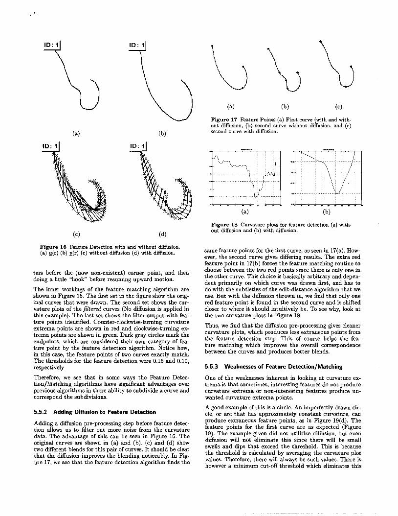
Figure 14 Comparing Path-Length Fraction Matching and Feature Matching Results. The red in (c) and (d) rep­resent the final blended result.

Point, Counter-Clockwise Curvature Extrema Point, and Endpoint. The algorithm attempts to minimize the number of DELETE and INSERT operations that would transform g into Q. While the resulting edit distance is the same for transforming Qinto g, it should be noted that the correspon­dence set that results may be different. There are always two Endpoint feature points for every curve, one at each end. The algorithm always ends up corresponding the endpoints correctly.

For the most part, this algorithm works well. However, it might be interesting to change the measurement of the edit distance so that deleting a feature of more severe curvature would require more than the usual one unit of edit distance. This might help correspond the correct features with each other. We have not had the time to implement such an al­gorithm. This would probably require doing the full-blown quadratic time algorithm for minimizing the edit distance, but the number of features is usually less than ten so effi­ciency does not seem like a problem.

5.4 Establishing Point Correspondence

After the feature points are matched up, we correspond the segment between each pair feature points using the CL or CT version of the Path-Length/Time Fraction Matching Algo­rithms in section 4.3. This method works quite well, assum­ing the right feature points were found and were matched up reasonably well.

In summary, the feature matching approach requires that we first do some filtering, analyze curvature data on the filtered curves to detect the relevant features, correspond the features, and lastly, correspond the points of the original curves.

ID: 0

(a) (d)

(b)

(c) (f)

Figure 15 Feature Matching without Diffusion. Y-axis is 0.2 radians per grid-line for (b) and (e).

5.5 Results

We now present our results for feature matching, analyzing how they work in more depth and comparing them with our earlier approaches.

5.5.1 Comparing Path Length Fraction and Feature Matching

Here we compare results from the Path-Length Fraction Matching Algorithm and the feature detection algorithm (without diffusion). In Figure 14, we draw two curves ((a) and (b)) and try to blend them. Note that, relative to the first curve, the second curve has longer path in its first sub­section and a shorter path in the second subsection." It is clear that since both !!(r) and y(r) contain a sharp "V" dip, the blended curve should as well. However, due to the slight shifting caused by the different arc lengths, the two corner points are not corresponded to each other in Figure 14(c). However, it's clear that in 14(d), the feature matching algo­rithm was able to find that critical point (because it's obvi­ously a curvature extrema) and correspond the points prop­erly. Not only is the blended shape better, but it could be that the user put a significant pause at the corner point. Us­ing the Path-Length Fraction Matching scheme, a replayed animation would result in the widget pausing a few millime­

4 A "subsection" is loosely defined to be however the "average" user would intuitively segment a motion path. In this example, there seem to be two subsections.

(e)

(a) (b)

10: 1

(c) (d)

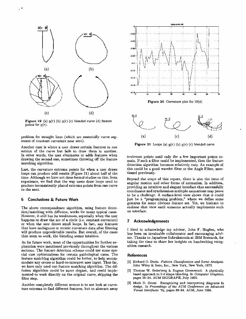
Figure 16 Feature Detection with and without diffusion. (a) :!f(r) (b) Q(r) (c) without diffusion (d) with diffusion.

ters before the (now non-existent) corner point, and then doing a little "hook" before resuming upward motion.

The inner workings of the feature matching algorithm are shown in Figure 15. The first set in the figure show the orig­inal curves that were drawn. The second set shows the cur­vature plots of the filtered curves (No diffusion is applied in this example). The last set shows the filter output with fea­ture points identified. Counter-clockwise-turning curvature extrema points are shown in red and clockwise-turning ex­trema points are shown in green. Dark gray circles mark the endpoints, which are considered their own category of fea­ture point by the feature detection algorithm. Notice how, in this case, the feature points of two curves exactly match. The thresholds for the feature detection were 0.15 and 0.10, respectively

Therefore, we see that in some ways the Feature Detec­tion/Matching algorithms have significant advantages over previous algorithms in there ability to subdivide a curve and correspond the subdivisions.

5.5.2 Adding Diffusion to Feature Detection

Adding a diffusion pre-processing step before feature detec­tion allows us to filter out more noise from the curvature data. The advantage of this can be seen in Figure 16. The original curves are shown in (a) and (b). (c) and (d) show two different blends for this pair of curves. It should be clear that the diffusion improves the blending noticeably. In Fig­ure 17, we see that the feature detection algorithm finds the

(a) (b) (c)

Figure 17 Feature Points (a) First curve (with and with­out diffusion, (b) second curve without diffusion, and (c) second curve with diffusion.

-

(a)

~ /

\ / ,

.

. II ... 10 » » .. . . (b)

Figure 18 Curvature plots for feature detection (a) with­out diffusion and (b) with diffusion.

same feature points for the first curve, as seen in 17(a). How­ever, the second curve gives differing results. The extra red feature point in 17(b) forces the feature matching routine to choose between the two red points since there is only one in the other curve. This choice is basically arbitrary and depen­dent primarily on which curve was drawn first, and has to do with the subtleties of the edit-distance algorithm that we use. But with the diffusion thrown in, we find that only one red feature point is found in the second curve and is shifted closer to where it should intuitively be. To see why, look at the two curvature plots in Figure 18.

Thus, we find that the diffusion pre-processing gives cleaner curvature plots, which produces less extraneous points from the feature detection step. This of course helps the fea­ture matching which improves the overall correspondence between the curves and produces better blends.

5.5.3 Weaknesses of Feature Detection/Matching

One of the weaknesses inherent in looking at curvature ex­trema is that sometimes, interesting features do not produce curvature extrema or non-interesting features produce un­wanted curvature extrema points.

A good example of this is a circle. An imperfectly drawn cir­cle, or arc that has approximately constant curvature, can produce extraneous feature points, as in Figure 19(d). The feature points for the first curve are as expected (Figure 19). The example given did not utilitize diffusion, but even diffusion will not eliminate this since there will be small swells and dips that exceed the threshold. This is because the threshold is calculated by averaging the curvature plot values. Therefore, there will always be such values. There is however a minimum cut-off threshold which eliminates this

6

(a) (b)

(c) (d)

Figure 19 (a) ~(r) (b) !!.(r) (c) blended curve (d) feature points for !!.(r).

problem for straight lines (which are essentially curve seg­ments of constant curvature near zero).

Another case is where a user draws certain features in one section of the curve but fails to draw them in another. In other words, the user eliminates or adds features when drawing the second one, sometimes throwing off the feature matching algorithm.

Last, the curvature extrema points for when a user draws loops can produce odd results (Figure 21) about half of the time. Although we have not done formal studies on this, from experience, we find that the way users draw loops tend to produce inconsistently placed extrema points from one curve to the next.

Conclusions &. Future Work

The above correspondence algorithm, using feature detec­tion/matching with diffusion, works for many typical cases. However, it still has its weaknesses, especially when the user happens to draw the arc of a circle (i.e. constant curvature) or when the user draws small loops. In fact, any features that have ambiguous or erratic curvature data after filtering will produce unpredictable results. But overall, of the cases that seem to work, the blending seems intuitive.

As for future work, most of the opportunities for further ex­ploration were mentioned previously throughout the various sections. The feature detection scheme could use some spe­cial case optimizations for certain pathological cases. The feature matching algorithm could be better, to help accom­modate any errors or hard-to-interpret user input. Thus far, we have only used one feature matching algorithm. The dif­fusion algorithm could be more elegant, and could imple­mented to work directly on the original curve, skipping the filter step.

Another completely different avenue is to not look at curva­ture extrema to find different features, but to abstract away

da1aourvalure8

-0.0

-0.04

-0.06

-0.08

-0.

-0.1

-0.1

-0.1

-0.1 o 10 20 30 40 60 60 70

2

~ A \ \

\Y\/\ \ ~ 1

\J A .. I v I

2 ,....

J4

6

6 ;

Figure 20 Curvature plot for 19(d)

(a) (c) (d)

Figure 21 Loops (a) ~(r) (b) !!.(r) (c) blended curve

irrelevant points until only the a few important points re­main. If such a filter could be implemented, then the feature detection algorithm becomes relatively easy. An example of this could be a good wavelet filter or the Angle Filter, men­tioned previously.

Beyond the scope of this report, there is also the issue of angular motion and other forms of animation. In addition, providing an intuitive and elegant interface that successfully coordinates and synchronizes multiple animations may prove to be a challenge. A surface-level view shows that it could just be a "programming problem," where we define some gestures for some obvious feature set. Yet, we hesitate to endorse that view until someone actually implements such an interface.

7 Acknowledgements

I liked to acknowledge my advisor, John F. Hughes, who has been an invaluable collaborator and encouraging advi­sor. Thanks to Jayashree Subrahmonia at IBM Research, for taking the time to share her insights on handwriting recog­nition research.

References

[1] Richard O. Duda. Pattern Classification and Scene Analysis. John Wiley & Sons, Inc., New York, New York, 1973.

[2] Thomas W. Sederberg & Eugene Greenwood. A physically based approach to 2-d shape blending. In Computer Graphics, pages 25-34. ACM SIGGRAPH, July 1992.

[3] Mark D. Gross. Recognizing and interpreting diagrams in design. In Proceedings of the ACM Conference on Advanced Visual Interfaces '94, pages 88-94. ACM, June 1994.

[4] James S. Lipscomb. A trainable gesture recognizer. Gesture Recognition, 24(9):895-907, 1991.

[5] Webb Miller and Eugene W. Myers. A file comparison pro­gram. Software-Practice and Experience, 15(11):1026-1040, November 1985.

[6] Dean Rubine. Specifying gestures by example. In Computer Graphics, pages 329-337. ACM SIGGRAPH, July 1991.

[7] Stuart Russell and Peter Norvig. Artificial Intelligence: A Modem Approach. Prentice-Hall, Inc., Upper Saddle River, New Jersey, 1995.

[8] Robert C. Zeleznik, Kenneth P. Herndon, and John F. Hughes. SKETCH: An interface for sketching 3D scenes. In SIG­GRAPH 96 Conference Proceedings, pages 163-170. ACM SIGGRAPH, August 1996.