


Languages
Pages
Legal


University of Texas at El PasoDigitalCommons@UTEP
Open Access Theses & Dissertations
2015-01-01
Simulation of Infiltrating Rate Driven By SurfaceTension-Viscosity of Liquid Elements from theTitanium Group Into a Packed BedArturo MedinaUniversity of Texas at El Paso, [email protected]
Follow this and additional works at: https://digitalcommons.utep.edu/open_etdPart of the Materials Science and Engineering Commons, Mechanical Engineering Commons,
and the Mechanics of Materials Commons
This is brought to you for free and open access by DigitalCommons@UTEP. It has been accepted for inclusion in Open Access Theses & Dissertationsby an authorized administrator of DigitalCommons@UTEP. For more information, please contact [email protected].
Recommended CitationMedina, Arturo, "Simulation of Infiltrating Rate Driven By Surface Tension-Viscosity of Liquid Elements from the Titanium GroupInto a Packed Bed" (2015). Open Access Theses & Dissertations. 1098.https://digitalcommons.utep.edu/open_etd/1098

SIMULATION OF INFILTRATING RATE DRIVEN BY SURFACE TENSION-VISCOSITY OF
LIQUID ELEMENTS FROM THE TITANIUM GROUP INTO A PACKED BED
ARTURO MEDINA
Department of Mechanical Engineering
APPROVED:
Arturo Bronson, Ph.D., Chair
Vinod Kumar, Ph.D.
David A. Roberson, Ph.D.
Charles Ambler, Ph.D.
Dean of the Graduate School

Copyright ©
By
Arturo Medina
2015

Dedication
This thesis is dedicated to all of my family for all of your love, support, and constant
encouragement throughout these years.
SIMULATION OF INFILTRATING RATE DRIVEN BY SURFACE TENSION-VISCOSITY OF
LIQUID ELEMENTS FROM THE TITANIUM GROUP INTO A PACKED BED
By
ARTURO MEDINA, B.S.
THESIS
Presented to the Faculty of the Graduate School of
The University of Texas at El Paso
in Partial Fulfillment
of the Requirements
for the Degree of
MASTER OF SCIENCE
Department of Mechanical Engineering
THE UNIVERSITY OF TEXAS AT EL PASO
May 2015

v
Acknowledgements
I would like to extend my greatest gratitude to God and to all my family, especially my
parents, sister, my aunt and my cousins that have always supported me when I needed it the most.
Your constant encouragement and advice have motivated me to be the person and engineer I am
today and words can never fully describe my admiration for all of you.
My biggest appreciation will, without a doubt, goes out to my mentor, advisor, committee
chair Dr. Arturo Bronson. He was the first to provide me with the opportunity to work in his high
temperature lab studying various metals at ultra-high temperatures. I know for a fact that I would
not be where I am today without his continuous support and sharing his vast knowledge he has
handed down to me. Through this support, he has assisted me in being accepted into two
internships through Kirtland Air Force Research Laboratory in the summers of 2013 and 2014.
Now, I am on my way to start my career with the Federal Aviation Administration and he was a
big reason for it. It was truly an honor to work with him in these past years.
I am also thankful for my time with Dr. Vinod Kumar and all those situations in his office
trying to figure out problems people have rarely thought about. Also, I am thankful for Dr. David
Roberson in accepting his role as a committee member for my thesis.

vi
Abstract
The simulation of infusion of molten reactive metals (e.g., yttrium) into a porous, carbide
packed bed to create carbide and boride composites was studied at ultrahigh temperatures
(>1700°C). The infusion was investigated through a computational fluid dynamic (CFD) system
of capillary pores and compared to a predicted analytical calculation formulated by Selmak and
Rhines. Simulations of two-phase flow penetration of yttrium into a packed bed of B4C were
investigated and compared with titanium, zirconium, hafnium, and samarium liquids. The non-
reactive, liquid metal infusion was primarily driven by the surface tension and viscosity. The liquid
metal depth and rate of penetration were determined and predicted at their respective melting
temperature to 2450°C. Along with these simulations and with the knowledge of the
thermophysical properties of each element, titanium shows the highest rate of penetration and
yttrium shows the lowest rate at their respective melting temperatures. However, once the
temperature starts to increase and the elements are observed at the same isothermal temperature,
yttrium begins to overtake the other elements in terms of depth and rate of penetration.

vii
Table of Contents
Acknowledgements ..................................................................................................v
Abstract .................................................................................................................. vi
Table of Contents .................................................................................................. vii
List of Tables ....................................................................................................... viii
List of Figures ........................................................................................................ ix
Chapter 1: Introduction ............................................................................................1
1.1 Overview ...................................................................................................1
1.2 Research Objective ...................................................................................2
Chapter 2: Literature Review ...................................................................................3
2.1 Infiltration and Surface Tension Driven Flow ..........................................3
2.2 Surface Tension .........................................................................................6
2.3 Contact Angle ...........................................................................................8
2.4 Pure Metal Physical Properties .................................................................9
Chapter 3: Methodology ........................................................................................13
3.1 FLUENT VOF Modeling ........................................................................13
Chapter 4: Results ..................................................................................................22
4.1 Elements at Melting Temperature ...........................................................22
4.2 Liquid Infusion under Isothermal Conditions .........................................30
4.3 Elements through Temperature Range....................................................36
Chapter 5: Discussion ............................................................................................39
5.1 Surface Tension – Viscosity Ratio ..........................................................39
5.2 Rate of Infusion.......................................................................................40
Chapter 6: Conclusion............................................................................................42
References ..............................................................................................................43
Vita .......................................................................................................................45

viii
List of Tables
Table 1-Physical Properties at Liquid Elements at Melting Temperature ...................................... 9 Table 2-Surface Tension - Viscosity Ratio at Melting Point and 2510K ..................................... 39 Table 3-Rate of Infusion at Melting Point and 2510K. ................................................................ 40

ix
List of Figures
Figure 1-Sketch of Contact Angle Resulting from Surface tension Forces between Phases .......... 8 Figure 2-Single Pore Geometry .................................................................................................... 14 Figure 3-Four-Pore Geometry....................................................................................................... 15 Figure 4-Single Pore Mesh ........................................................................................................... 16 Figure 5-Four Pore System ........................................................................................................... 16
Figure 6-Boundary Conditions of the Single Pore. ....................................................................... 19 Figure 7-Interface Calculations [8]. .............................................................................................. 20 Figure 8-Depth of Penetration of Ti at Melting Point................................................................... 23
Figure 9-Maximum Depth of Four Pore System for Ti ................................................................ 24 Figure 10-Depth of Penetration of Zirconium at Melting Point. .................................................. 25 Figure 11-Maximum Depth of Four Pore System of Zr. .............................................................. 25 Figure 12-Depth of Penetration of Hf at Melting Point. ............................................................... 26
Figure 13-Maximum Depth for Four Pore System of Hf ............................................................. 27 Figure 14-Depth of Penetration of Y at Melting Point. ................................................................ 28
Figure 15-Maximum Penetration for Four Pore System of Y ...................................................... 28 Figure 16-Depth of Penetration of Sm at Melting Point. .............................................................. 29
Figure 17-Maximum Depth of Penetration at Melting Point ........................................................ 30 Figure 18-Depth of Penetration of Ti at 2510K ............................................................................ 31 Figure 19-Maximum Penetration of Ti at 2510K ......................................................................... 31
Figure 20-Maximum Depth of Penetration at 2510K ................................................................... 32
Figure 21-Maximum Depth of Penetration at 2510K ................................................................... 33 Figure 22-Depth of Penetration of Hf at 2510K ........................................................................... 34 Figure 23-Maximum Depth of Hf at 2510K ................................................................................. 34
Figure 24-Depth of Penetration of Y at 2510K ............................................................................ 35 Figure 25-Maximum Penetration of Y at 2510K .......................................................................... 36
Figure 26-Rate of Penetration from 1700°C to 1900°C for Ti and Y ........................................... 37
Figure 27-Rate of Penetration from 2250C to 2450C for Ti and Y. ............................................. 38
Figure 28- Depth of Penetration of Elements at Melting Point .................................................... 39 Figure 29- Depth of Penetration of Elements at 2510K ............................................................... 40
Figure 30-Rate of Infusion at Melting Point of Elements............................................................. 41 Figure 31-Rate of Infusion of Elements at 2510K ........................................................................ 41
1
Chapter 1: Introduction
1.1 Overview
The reactive infusion of molten metals into a porous powder to create carbide and boride
composites are extremely advantageous because the ultimate near-net product may have
compounds capable of usage at ultrahigh temperatures. Johnson, Nagelberg, and Breval [1] have
initially reported the reactive infusion of liquid Zr into a packed bed of B4C; with the expanding
use of liquid reactive metals, the techniques can produce ultrahigh temperature ceramics. These
ceramics are often known for their high melting points, high hardness, and good oxidation
resistance especially the transition metal groups IV and V [2]; these metals include titanium (Ti),
zirconium (Zr), hafnium (Hf), and yttrium (Y) and will be investigated in this study. Because of
their high negative free energies, these create great stability under extreme conditions and make
them ideal in high temperature applications. For these reasons, UHTCs are used largely in the
aerospace industry involving in development of turbine blades as well as airframe leading edges
for reentry vehicles.
Nonreactive liquid, metal infiltration involving the core elements of Hf, Zr, Ti, Y, and
Samarium penetrating into a packed bed is being investigated at ultrahigh temperatures (>1600oC).
Infiltration is a term often reported by Selmak and Rhines [3] when investigating molten metal
filling a porous body through capillary forces. The forces being considered are heavily driven by
the liquid/gas surface tension and the viscosity of the molten metal without any interfacial
reactions. The assumption of nonreactive wetting is also important factor in creating a metal-B4C
matrix as it will determine the surface tension-viscosity effects on the penetration of the liquid.
Halverson et al [4] explained the grave difficulty when molten aluminum infiltration into the B4C
powder is ceased does not achieve optimal wetting. They noted the importance of the contact angle,
θ; meaning that <90° needed for and to differentiate a non-wetting fluid.
Computational effort is the main focus in predicting the infiltration to give a comparison
to the experimental setup. Fluent, a computational fluid dynamics (CFD) software based on a finite

2
volume method, is implemented with elemental surface tension to study the micro-scale pore
system. To determine the depth of penetration, which must be accounted for, a volume of fluid
(VOF) multiphase model was utilized. This model applies and considers the transient tracking of
the liquid-gas interface (i.e. metal-carbon dioxide) that will be of great value in penetration into
the porous media.
1.2 Research Objective
The objective of the present study predict the rate of infusion of the pure elements (Hf, Ti,
Y, Zr, and Sm) into a porous B4C using computational fluid dynamic software (i.e. ANSYS Fluent)
and compare them with pervious theoretical and experimental findings. The key parameters of
surface tension, viscosity pore characteristics and temperature will be used to determine the
optimal penetration of the liquid metal into a packed bed. The research findings will then enable
future studies to build on the effects of reactive wetting on penetration.

3
Chapter 2: Literature Review
In the review of the surface-tension, driven infiltration of molten metals into a porous
material, the discussion will begin with the explanation of liquid elements used in the simulations
and thermophysical properties needed to determine their flow. The reactive materials i.e., Ti, Hf,
Y, Zr, and Sm will infiltrate the pores of a packed bed of B4C. The properties of each metal
investigated will be characterized over a temperature range starting from each respective melting
temperature and ending at 2450°C by considering critical parameters including surface tension,
contact angle, viscosity, and density. Selmak and Rhine [3] is used a porous metal powder and
infiltrated a relatively low melting (< 1000°C) temperature pure metal determining a depth of
penetration and a rate of infusion. Ligenza and Bernstein [5] utilized Poiseuille’s law, a differential
equation, in which describes the physical phenomena of capillary flow. Martin and his team [6]
combine the findings of Selmak-Rhines and Ligenza-Bernstein to create an equation for modeling
the kinetics of liquid-metal infiltration. The discussion of surface-viscosity driven flow will be
explained more thoroughly by past experiments and computationally simulated examples.
2.1 Infiltration and Surface Tension Driven Flow
The main focus of this project is heavily relied on the term of infiltration which can predict
the flow of liquid metal into a packed bed of B4C. There are many factors to consider in this
phenomena of a liquid metal penetrating a packed bed. At ultrahigh temperatures, these liquid
metals experience a multitude of temperature gradients, exothermic reactions, diffusion,
differentiating contact angle, and experience variations of their physical properties [7].
2.1.1 Capillary Flow
As previously mentioned, the research conducted by Ligenza and Bernstein utilized a
mathematical model to represent liquid rise in fine capillary tubes with radii consisting 20 to 50µm
[5]. They gather that Poiseuille’s law with the assumption of non-stationary state, and the wetting
is very rapid, brings into a differential equation of motion (1).

4
𝑑
𝑑𝑡{𝜋𝑅2[𝜌ℎ + 𝜌𝑎(𝑙 − ℎ)]
𝑑ℎ
𝑑𝑡}
= 2𝜋𝑅𝜎𝑐𝑜𝑠𝜃 − 8𝜋𝑑ℎ
𝑑𝑡[𝜂ℎ + 𝜂𝑎(𝑙 − ℎ)] − 𝜋𝑅2𝑔ℎ(𝜌 − 𝜌𝑎)
−1
4𝜋𝑅2𝜌 (
𝑑ℎ
𝑑𝑡)
2
(1)
Where h is the height (or depth) of the column of liquid within the time t, with R and l
being the radius and length of the capillary, η and ηa are the viscosity of the liquid and of the air
respectively, ρ and ρa are the density of the liquid and air. While σ is the liquid-gas surface tension
and θ is the contact angle, assumed to be constant. The term on the left side of the equation is the
rate of change of momentum while the terms on the right are, respectively, forces due to surface
tension, viscous resistance, gravity, and the “end-drag effect”.
A manipulation of this equation was later investigated by Selmak and Rhines [3] observing
their measurements involving a low melting temperature metal penetrating through a porous higher
melting temperature metal structure. The validity of a simplification of equation (1) was originally
established by the pervious experimentation done by Ligenza and Bernstein hypothesizing that the
rate of change of momentum and end-drag effect terms can be neglected. This is due to the
sufficiently small radius of the tube that the rate of the depth of penetration may be slow enough
to disregard. Also, the viscosity and density of the air (or any gaseous compound) will be two to
three orders of magnitude smaller than the liquid penetrating into it. After all the assumptions are
made equation (1) reduces to:
Where a relationship of surface tension, σ, divided by viscosity, η, can be developed with
the assumption that all liquid metals with penetrate into the same porous capillary radius, R,
wetting parameters, θ, and time, t. The determination of 𝜎
𝜂, which is known as a characteristic
velocity having the units distance over time, brings in a new representation of how much a liquid
metal will penetrate into a packed bed. Further discussion about this characteristic velocity will be
evaluated when taking specific metals into consideration.
ℎ = √𝑅𝜎 cos 𝜃 𝑡
2𝜂 (2)
5
A relationship with the depth of penetration being formulated, a rate, 𝑑ℎ
𝑑𝑡, is determined by
differentiating the equation (2) as a function of time. The following shows that:
𝑑ℎ
𝑑𝑡=
1
2√
𝑅𝜎 cos 𝜃
2𝜂 𝑡 (3)
Where the main difference would be the parameter of time, t. Given that time is in the denominator
of the equation, one should note that at t=0, 𝑑ℎ
𝑑𝑡= ∞.
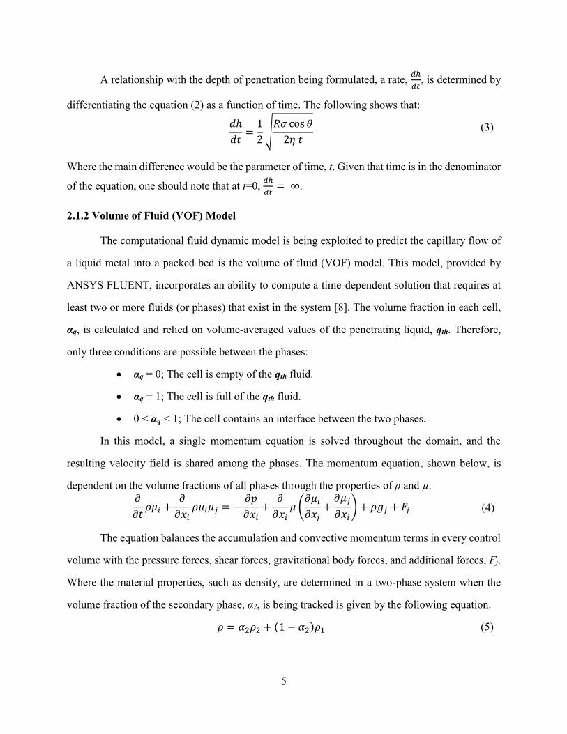
2.1.2 Volume of Fluid (VOF) Model
The computational fluid dynamic model is being exploited to predict the capillary flow of
a liquid metal into a packed bed is the volume of fluid (VOF) model. This model, provided by
ANSYS FLUENT, incorporates an ability to compute a time-dependent solution that requires at
least two or more fluids (or phases) that exist in the system [8]. The volume fraction in each cell,
αq, is calculated and relied on volume-averaged values of the penetrating liquid, qth. Therefore,
only three conditions are possible between the phases:
αq = 0; The cell is empty of the qth fluid.
αq = 1; The cell is full of the qth fluid.
0 < αq < 1; The cell contains an interface between the two phases.
In this model, a single momentum equation is solved throughout the domain, and the
resulting velocity field is shared among the phases. The momentum equation, shown below, is
dependent on the volume fractions of all phases through the properties of ρ and µ.
𝜕
𝜕𝑡𝜌𝜇𝑖 +
𝜕
𝜕𝑥𝑖𝜌𝜇𝑖𝜇𝑗 = −
𝜕𝑝
𝜕𝑥𝑖+
𝜕
𝜕𝑥𝑖𝜇 (
𝜕𝜇𝑖
𝜕𝑥𝑗+
𝜕𝜇𝑗
𝜕𝑥𝑖) + 𝜌𝑔𝑗 + 𝐹𝑗 (4)
The equation balances the accumulation and convective momentum terms in every control
volume with the pressure forces, shear forces, gravitational body forces, and additional forces, Fj.
Where the material properties, such as density, are determined in a two-phase system when the
volume fraction of the secondary phase, α2, is being tracked is given by the following equation.
𝜌 = 𝛼2𝜌2 + (1 − 𝛼2)𝜌1 (5)

6
Since the determination of surface tension being a great factor in the penetration flow, Fj
will result in the surface tension force added into equation (3). The VOF model can incorporate
the effects of surface tension along the interface between each pair of phases and also by
augmented by a specification of the contact angle between the phases and walls. The surface
tension model in the CFD program utilizes the continuum surface force (CSF) model proposed by
Brackbill et al. [9]. When the surface tension is taken to be a constant along the surface, the only
forces normal to the interface are considered. The surface curvature as measured by two radii in
orthogonal directions, R1 and R2, making the pressure drop across the surface to depend on the
surface tension coefficient, σ. The equation below expresses this relationship:
𝑝2 − 𝑝1 = 𝜎 (1
𝑅1+
1
𝑅2) (6)
Also, the VOF model gives an option to specify a wall adhesion angle in accordance with
the surface tension model. There is a contact angle that the fluid is assumed to make with the wall
and uses that information to adjust the surface normal to in the cells near the wall. The following
equation is used to determine the adjusted curvature near the wall:
�̂� = �̂�𝑤 cos 𝜃𝑤 + �̂�𝑤 sin 𝜃𝑤 (7)
Where �̂�𝑤 and �̂�𝑤 are the unit vectors normal and tangential to the wall, respectively. The
contact angle is represented as 𝜃𝑤 where this terms helps determine the adjusted body force term
in the surface tension calculation.
2.2 Surface Tension
The liquid property of surface tension is often described as the result of a force acting on
a plane and how much that force of attraction is to the bulk, or substrate [10]. The surface tension
of a liquid metal is a crucial property to know and is closely associated with liquid metal processing
[11]. This property plays an important role in interfacial flow especially in the micro-scale. The
liquid has molecules that are continually held together by cohesive forces, especially in the bulk;
the molecules on the edge of the liquid are weaker because it is not surrounded by similar
molecules. Depending on how strong of a force it takes to break these molecules apart gives the

7
name to surface tension. So far, the applications that heavily involved surface tension driven flow
have been ink-jet, thermal spray coating industries, and metal matrix infiltration procedures.
2.2.1 Determining Surface Tension
Extensive research has been done for determining the surface tension of high temperature
melting metals with the drop-weight method and non-contact techniques being reviewed in this
paper. Peterson and his team [11] investigated the surface tensions of liquid Ti, Zr, and Hf at their
respective melting temperatures using this method. The method introduces a hanging liquid drop
that is made at the end of a cylindrical rod and grows until it falls due to its weight. The surface
tension, σ, of the molten metals are then calculated by the following equation:
𝜎 =𝑚𝑔𝐹
𝑟 (8)
The parameters include mass, m, acceleration due to gravity, g, radius of the rod, r, and
correction factor, F.
Another technique is involving no contact with the metal called high temperature
electrostatic levitation. Paradis and his team at Jet Propulsion Laboratory [12] investigation
consists of a stainless steel chamber which is evacuated to 10-8 Torr before any temperature
ramping began. The samples were spherical in shape and place between two, parallel plate
electrodes and then directed into a He-Ne laser beam to maintain its shape. The sample was then
heated utilizing an Nd-YAG laser to achieve the melting temperature and keep it stable. Surface
tension can be determined once the characteristic oscillation frequency, ωc, of the sample was the
determined.
Aqra et al. [13] propose a theoretical model and use relations for calculating the surface
tension and the differential surface tension with respect to temperature of liquid metals at any
temperature and compare them to techniques already used in previous experimentation. The
formation of the solid-vapor interfacial tension in the calculations are difficult to calculate as the
model depends on previous experimental data. The temperature dependence of the solid-liquid
interaction of pure metals was also computed and scaled with the elements melting point showing

8
agreement with experiment values [15]. Hondros [16] explains the importance of the interfacial
energies in solids and gave estimated values through the grain boundaries of pure metals.
2.3 Contact Angle
The contact angle, or the wetting of
molten metal onto a packed bed is a great
determination of infiltration. Delannay and his
team [7] review the significance of the concept
of wetting of solids by liquid metals in metal-
matrix composites. Wetting is the ability of a
liquid to keep in contact with the solid substrate
[14]. This parameter is the best determining
factor for wetting between the liquid and the
interacting surface, or substrate it is exposed to.
Studies of wettability have been conducted with pure liquid metals on a substrate of beryllium and
how those elements react and relate to each other [17]. When a liquid reaches an equilibrium with
the solid it is in contact with, an angle, θ, can be determined between the liquid and solid phase.
Figure 1 shows a schematic of a drop of liquid onto a solid substrate in a gaseous environment
after equilibrium has been achieved. When the liquid metal is in complete wetting, partial wetting,
or non-wetting, the angle is assumed to be 0°, 0 < θ < 90°, and 90° respectively [19]. The balance
of forces in surface tension with respect to the contact angle can be shown below:
𝜎𝑠𝑣 = 𝜎𝑙𝑠 + 𝜎𝑙𝑣𝑐𝑜𝑠𝜃 (9)
The Young-Duprè equation, which considers the forces acting on the point of intersecting
lines for the solid/gas (σsg), liquid/solid (σls), liquid/gas (σlv) interfaces, can be used to acquire a
contact angle when none is known. By rearranging equation (9), it shows:
Figure 1-Sketch of Contact Angle Resulting
from Surface tension Forces
between Phases

9
Studies conducted by Saiz and Tomsia [20] review the phenomena of both low and high
temperature wetting and spreading rates. They reveal various effects of oxygen partial pressures
and absorption occurrences along the triple-line of liquid, gas, and solid. Also, researchers have
considered rates of spreading in Al2O3/Fe-42Ni substrates in the drop transfer set-up to gather
more information of the dependence of the parameter of the contact angle [21].
2.4 Pure Metal Physical Properties
Determining the physical properties of these transition metals at their molten states is very
important when evaluating and predicting penetration rate through a packed bed. Though very
vigorous, the teams of Peterson and Paradis have done extensive research and experimentation to
evaluate this properties at these extreme conditions [12], [19]. The previous section explains
specifically about the importance of surface tension and contact angle, however, viscosity and
density play a factor in material selection as well as the rate of infusion in a packed bed of B4C.
Researchers have also tried determining the viscosity using theoretical models for pure metals
[17]. Below, table 1 shows the selected elements that have been chosen in predicting a depth of
penetration. This section will also discuss the specific elements physical properties in a linear
relationship with respect to a range of temperatures.
Table 1-Physical Properties at Liquid Elements at Melting Temperature
Element
Melting
Temperature
K (°C)
Parameters at Melting Temperature
Surface
Tension (σmp)
Nm-1
Viscosity (ηmp 103)
kgm-1s-1
Density
(ρmp 10-3)
kgm-3
σmp/ηmp
ms-1
Hafnium 2504 (2231) 1.614 5.12 12.00 315.2
Titanium 1941 (1668) 1.557 4.42 4.208 352.3
Samarium 1347 (1074) 0.430 2.29 7.015 188.1
Yttrium 1795 (1522) 0.804 4.54 4.150 177.1
Zirconium 2128 (1855) 1.500 4.74 6.240 316.5
𝜃 = 𝑐𝑜𝑠−1 (𝜎𝑠𝑣 − 𝜎𝑙𝑠
𝜎𝑙𝑣) (10)

10
2.3.1 Pure Titanium
As explained above, the procedure of non-contact measurements utilizing an electrostatic
levitation furnace determined the surface tension (11), viscosity (12), and density (13) of pure
molten titanium. By using this technique, a linear relationship was formed into the properties as a
function of temperature where Tm=1943K [22], [23]. The follow equations below express this
relationship:
𝜎(𝑇) = 1.557 × 10³ − 0.156(𝑇 − 𝑇𝑚) (11)
𝜂(𝑇) = 4.420 − 6.67 × 10⁻³(𝑇 − 𝑇𝑚) (12)
𝜌(𝑇) = 4.208 × 10³ − 0.508(𝑇 − 𝑇𝑚) (13)
2.3.2 Pure Zirconium
The procedure of non-contact measurements have been used in determining the
thermophysical properties of the molten state of zirconium. Even though Zr has a high melting
point and good corrosion resistance, there is a high risk of contamination of the samples when the
temperatures reach the liquid temperature [15]. These properties of surface tension (14), viscosity
(15), and density (16) are determined by the linear equations with respect to temperature expressed
below:
𝜎(𝑇) = 1.459 × 10³ − 0.244(𝑇 − 𝑇𝑚) (14)
𝜂(𝑇) = 4.83 − 5.31 × 10⁻³(𝑇 − 𝑇𝑚) (15)
𝜌(𝑇) = 6.24 × 10³ − 0.29(𝑇 − 𝑇𝑚) (16)

11
2.3.3 Pure Yttrium
Yttrium also has a great challenge in measuring the thermophysical properties in the fact
that it has a high vapor pressure and the risk of contamination of its liquid state. Using the
electrostatic levitation and non-contact techniques allowed the determination of the properties in
at molten temperatures [25]. A relationship with respect to temperature was defined for surface
tension (17), viscosity (18), and density (19) through the following equations:
𝜎(𝑇) = 8.04 × 10² − 0.05(𝑇 − 𝑇𝑚) (17)
𝜂(𝑇) = 0.00287𝑒𝑥𝑝 [1.1 × 10⁵
𝑅𝑇] (18)
𝜌(𝑇) = 4.15 × 10³ − 0.21(𝑇 − 𝑇𝑚) (19)
2.3.4 Pure Hafnium
The processing of this material is extremely difficult because in nature, it is mostly present
in zirconium minerals. As an effect to this, the properties are largely affected by the impurities of
zirconium in hafnium; the difficultly comes from the production side as the two elements are
challenging to separate. Chemically speaking, they are very identical, however, hafnium’s density
is almost twice of that of zirconium.
Non-contact measurements were used in Hafnium [26]. Once again, a linear relationship
was calculated to give these thermophysical properties as a function of temperature. The following
equations below:
𝜎(𝑇) = 1.614 × 10⁻³ − 0.100(𝑇 − 𝑇𝑚) (20)
𝜂(𝑇) = 0.495 𝑒𝑥𝑝 [48.65 × 10³
𝑅𝑇] (21)
𝜌(𝑇) = 12.0 × 10³ − 0.44(𝑇 − 𝑇𝑚) (22)

12
2.3.5 Pure Samarium
Even though limited research has been conducted in the investigation of pure samarium,
there are still some thermophysical properties evaluated at its melting point. Non-contact
techniques were used in determining the surface tension of Sm creating a linear relationship as a
function of temperature through the following equation [27]:
𝜎(𝑇) = 430 − 0.072(𝑇 − 𝑇𝑚) (23)
A viscosity model was determined by Iida and Guthrie [16] by using dimensionless
parameters determined on the basis of predicted sound velocities. The following equation shows
viscosity (24) of liquid samarium at its melting point:
𝜂𝑚 = 0.369𝑀1/2𝜎𝑚
(𝜉𝑇𝑇𝑚)1/2 (24)
The density of samarium was measured by Stankus and his team [17] using a method of
irradiating the samples by a narrow beam of monochromatic gamma-rays. The following equation
shows a linear relationship with respect to temperature calculated through the liquid density (25)
data:
𝜌(𝑇) = 7015 − 1.019(𝑇 − 𝑇𝑚) (25)

13
Chapter 3: Methodology
The thought process in investigating the penetration of pure molten metals into a packed
bed of B4C starts by building a model that is compared with the Selmak-Rhines equation
mentioned above in equation (1). By using the CFD finite volume element method, incorporated
into the ANSYS FLUENT software, a one-pore and a more complex four-pore system were used
to simulate liquid metal penetrating into a packed bed. The five interested pure reactive elements,
i.e. Ti, Zr, Hf, Sm, and Y, were investigated at their respective melting points. Also, the fluid flow
penetration at an isothermal temperature of 2510K (2237°C) was simulated for a more realistic
comparison. The rate of penetration adjusts because the physical properties change within a range
of temperature. Using this information, the liquid pure elements were also compared from a
temperature range of 1700°C to 1900°C for Ti and Y, and from 2250°C to 2450°C for Zr and Hf.
There were a few major assumptions in the calculation and prediction of penetration depth and
rate that need to be mentioned. The following assumptions are:
i. Non-reactive infiltration.
ii. No temperature gradients throughout the geometry.
iii. Metal wetting at the surface/liquid interface.
iv. Homogenous pore size in the simulated packed bed.
In the following sections, the computational designs are summarized to predict depth and
rate of penetration were simulated and compared with the Selmak-Rhines equation mentioned
above. A pore network model with more complex pores was also developed to compare the rate
and depth of penetration, as outlined as the final methodology of the thesis.
3.1 FLUENT VOF Modeling
3.1.1 Geometry
Two main geometries were designed and utilized for modeling of the fluid flow through a
capillary tube. The first being a single 10µm pore connected above it to a reservoir of the liquid
metal above allowing it to wet into the pore. The second design was based on a four vertical pore

14
system, however, it will include intermediate pores that intersect the four pores perpendicularly
causing the fluid to flow with more restricting obstacles.
3.1.1.1 Single Pore System
The single pore system consisting of a 10µm
pore connected to reservoir (on top).As shown in Figure
2, the 20µm x 10µm reservoir of the single pore system
was just large enough to give a housing for the liquid
element to enter through. The length of the pore
measured at 500µm to give enough room for the liquid
metal to penetrate within the given time. This system
allows a similar comparison with equation (1) which
assumes only one liquid element flowing into a straight
capillary tube. Even with the geometry’s simplistic
nature, Selmak-Rhines predicted correctly the rise or depth of a liquid metal into a straight capillary
tube [3].
Figure 2-Single Pore Geometry

15
3.1.1.2 Four-Pore System
The four pore system
mimicked a more complicated
system of flow than liquid metal
flowing into one straight
capillary pore. The main
principles still apply and
resemble the single pore system.
The reservoir of the complicated
four-pore system is a little wider
at 80µm x 10µm to house the
liquid metal penetrating into the
pores below. The total length of
the vertical pores are at 600 µm to allow plenty of space for the liquid metal to flow within the
given time frame. The simulated packed bed was assumed as homogenous, meaning that all the
pore diameters are equal to each other. The pore diameter chosen was the same as for the single
pore system of 10 µm consistent with the pores of an experimental packed bed of B4C. A staggered
layout in the space between the four main vertical pores was designed; one having a 100µm of
space in between the intermediate pores while the center of the design having a 50 µm of space
between those smaller pores, as shown in figure 3. The staggered design gives a sense of
randomness for the smaller pores connecting to the vertical pores as the liquid metal penetrated.
The design was repeated throughout the whole 600 µm length of the system creating a simplified
packed bed of boron carbide.
3.1.2 Mesh
The meshing aspect plays an important role in calculating not only the penetration of the
liquid metal, but also the accuracy of the model as a whole. A multitude of factors (e.g.,
Figure 3-Four-Pore Geometry

16
computational expense, accuracy, and knowing the physical aspect of the geometry) plays into a
good mesh design. The decision was not simply on how fine a mesh to create, but depended on the
geometry for the calculation. The two geometries explained above, obviously accommodated the
liquid into the pores.
3.1.2.1 Single Pore System
The single pore system has a fine mesh of quadrilaterals throughout the entire geometry,
as shown in figure 4. Each node on the edge of the walls had an even spacing of 0.4 µm totaling
to 29995 nodes in the pore and reservoir. Once the mesh was generated, a total of 28820 element
cells were involved throughout the system (i.e., only 1269 cells are represented in the reservoir
while 27551 at the single pore). The mesh design amounts to makes 96% of the element cells were
located at the pore, where the calculation and physical area is of great interest.
Figure 4-Single Pore Mesh
Figure 5-Four Pore System
3.1.2.2 Four Pore System
Since this structure was vastly larger and more complex than the previous one explained,
the mesh needed more enhancement. As in the single pore system, the four pore system had a fine
mesh of quadrilaterals throughout most of the system, but also a hybrid of triangular cells to

17
optimize the layout of the geometry. This was due to the randomness created in the intermediate
pores as they were not uniform and staggered through the length of the pore. The nodes have a
spacing of 0.4 µm along the walls of every pore and the reservoir above totaling to a number of
172,490 nodes. A mesh with total of 166,294 element cells are generated (i.e., 5040 cells being
located at the liquid metal reservoir while 161,254 cells at the pore structure below it). The cells
generated amounted to 97% the area of where the penetration was located, i.e. the pore
arrangement.
3.1.3 Solution Setup
The single pore and the four pore system were both analyzed through the same solution
setup through the CFD program ANSYS FLUENT for each pure element being investigated.
Setting the initial steps included the solver and additional physics models, establishing the
materials and phases within the system, boundary conditions, solution methods and initialization,
and finally calculating the simulation. All these steps were essential in providing an accurate and
repeatable model for the system and explained fully in this sub-section.
3.1.3.1 Solver and Models
The system was constructed on a pressure-based solver meaning that the liquid metal was
assumed to be incompressible, or density is constant with respect to time, and at a relatively low
velocity. The method was the momentum equation to obtain a velocity field which was extracted
by solving a pressure correction equation by manipulating the continuity and momentum equations
[8].
By using the VOF model (as explain in Chapter 2), a time-dependent, transient-state,
solution is was selected to track the interface of the two phases, liquid metal and the gas. The
modeling allowed gives the ability to see how the depth of the fluid goes into the single or four
pore structure with respect to time.

18
3.1.3.2 Materials and Phases
In each given simulation, one pure liquid element was driven into the pore structure by
surface tension. As stated in Chapter 2, the pure elements were investigated at their respective
melting temperatures along with an isothermal temperature for Ti, Hf, Zr, Y, and Sm. The second
fluid in contact with the liquid metal carbon monoxide (CO) gas and initially filled the pores at
time of zero. The materials were defined by three preliminary characteristics which include density
(ρ), viscosity (η), and surface tension (σ) at the temperature.
In a two-phase system, the CFD program recognized and required an input of a primary
and a secondary phase. The primary phase consists of the defending fluid, CO gas, which was
already contained in the pores at the initial time. The secondary phase was left to the liquid metal
which initially did not penetrated into the pores and was located at the reservoir. Also an interaction
parameter focused on the surface tension with wall adhesion of the secondary fluid and is an
important factor with our calculation of the flow.

19
3.1.3.3 Boundary Conditions
Three main boundary conditions were set when studying the flow
of the penetrating molten metal. Since the main flow was driven by surface
tension and no injecting rate applied, the inlet (the opening at the top of the
reservoir) was defined as a pressure-inlet. Similarly, the lowest part of the
pore was defined as a pressure-outlet where a pressure gradient was
established. The final boundary condition was at the pore walls giving a
parameter “wall” at other every edge.
Subsequently, the pressure defined in the inlet and outlet of the two
systems was zero, since no other external forces are acting upon the liquid
metal; this gives a zero pressure gradient throughout the entire system. At
each of the walls of the pore, a constant contact angle
between the liquid metal and the wall were set at a wetting
angle of five degrees. The exact locations of the foregoing
boundary conditions for CFD model are shown in figure 6. For the four pore system, the same
boundary conditions as the single pore design were used the simulations repeatable for each
different liquid element.
3.1.3.4 Solution Methods and Initialization
The pressure-velocity coupling scheme used on both the single and four pore system was
the Pressure-Implicit with Splitting of Operators (PISO) approximating the relationship between
the corrections for pressure and velocity. This algorithm takes a little more computational time per
iteration, but in transient problems.
The Spatial Discretization used in the simulations have four major sections in the gradient,
pressure, momentum, and volume fraction. The least squares cell-based gradient evaluation was
selected in the gradient section which considers the solution to vary linearly through the center of
each cell, as is shown through equation (26).
Figure 6-Boundary Conditions
of the Single Pore.

20
(∇𝜙)𝑐0 ∙ ∆𝑟𝑖 = (𝜙𝑐𝑖 − 𝜙𝑐0) (26)
This expression represents that from the center of cell c0 to cell ci, a change in the cell
values between cell c0 and ci occurs along the vector Δri [8]. This assumption happens throughout
every neighboring cell at a given time-step.
In the pressure section, the PRESTO! (PREssure STaggering Option) was chosen since the
scheme uses a discrete continuity balance for a “staggered” control volume. This help with the
current problem as the interface of the liquid metal and gas create a curved shape throughout the
pores of the system.
For the momentum section of the spatial discretization solution, a second-order upwind
was selected to achieve a higher-order of accuracy in the momentum equation. A Taylor series
expansion of the cell-centered solution about the cell centroid was used to calculate equation (27)
[8].
𝜙𝑓,𝑆𝑂𝑈 = 𝜙 + ∇𝜙 ∙𝑟 (27)
This expression shows that ϕ and ∇ϕ
are the cell-centered value and its gradient in
the upstream cell, and 𝑟 is the displacement
vector from the upstream cell centroid to the
face centroid. Note, that this formulation
requires the determination of ∇ϕ and was
mentioned in equation (26).
Lastly, the volume fraction section
was used to give a special interpolation from
the cells that lie near the interface between
the two phases, i.e., the pure liquid element Figure 7-Interface Calculations [8].
21
and the CO gas. The geometric reconstruction scheme was used in this instance as it gives a more
accurate shape compared to the donor-acceptor scheme shown in figure 7. The geometric
reconstruction great accuracy was based on the assumption that the interface between two fluids
has a linear slope within each cell. It uses the linear shape to calculate an advection through the
fluid in the cell faces giving the overall shape in the domain.
Once every solution method was decided, the initialization of the system was then created
to start the calculation. The liquid element had to be put into the reservoir section before every
calculation run. This was accomplished by adapting a region of the reservoir space above the pore
and patching the liquid metal phase into the marked region. This gives an initial setting to the
liquid metal to wet into the pore and flow.
3.1.3.5 Calculation Utilization
After initialization of the solution for the system, running the solution consists of creating
a time step size, with the unit of seconds (s). Since the mesh size and overall size of the geometry
is in the micro-scale, the time-steps of the solution must be in the micro-scale. For this reason and
to achieve solution stability, the time-step size chosen was 1 × 10⁻⁸seconds. The number of time
steps have also been evaluated to be at 10,000 giving a flow time of 100 µs when the solution is
complete.

22
Chapter 4: Results
The two pore designs mentioned in the previous chapter were thoroughly used in predicting
the depth and rate of penetration of liquid elements into a packed bed of B4C. Simulations with the
one pore design were distributed at the melting temperatures of each element and were first
investigated to compare the outcomes to theory. Each metal was compared to each other as well
to see the effects of their different properties on the depth and rate at similar conditions. Once
those were simulated, the four pore design was then used to understand the depth and rate of
penetration through the structure created at each metal’s melting temperature; each of the liquid
element’s physical properties were calculated temperature region required. A maximum depth was
measured on the four pore design to obtain the most accurate results from the system. The
simulations were executed through a temperature range from 1700°C to 1900°C for titanium and
yttrium and for the higher melting elements of hafnium and zirconium from 2250°C to 2450°C
was chosen.
4.1 Elements at Melting Temperature
The simulations at melting temperatures served as an initial reference when the metal first
penetrated through the packed bed of B4C. Each liquid was simulated through a flow time from 10
µs to 100 µs. The Selmak-Rhines equation was used to compare the results from simulated with
computational fluid dynamics (CFD) for liquid metal penetration into the one or four pore systems.
4.1.1 Titanium
4.1.1.1 One Pore System
The depth penetration determined by CFD was slightly less than analytical by Selmak-
Rhines equation as shown in figure 8. The penetration calculated by the CFD at 100 µs is 0.278
mm while the depth of the theoretical equation puts a value of 0.296mm. A rate of penetration of
the single pore system was also calculated with the data of Figure 8. The rate from CFD from

23
simulations determined 1.14 m/s at the time of 100 µs while the rate from Selmak-Rhines 1.48
m/s.
4.1.1.2 Four Pore System
The maximum depth of penetration of titanium in a four pore system increases quickly
from 0.034 mm though the first 60 µs and holds relatively steady at 0.242 mm for the rest of the
simulation until 100 µs as shown in Figure 9. The penetrating rate for Ti through the four pore
system is the highest of all the elements. At 100 μs, the rate of penetration of 1.26 m/s was
calculated for Ti from Figure 9.
Figure 8-Depth of Penetration of Ti at Melting Point.
0
0.05
0.1
0.15
0.2
0.25
0.3
0.35
0 20 40 60 80 100 120
De
pth
(m
m)
Time (µs)
Titanium
Selmak-Rhines
CFD

24
Figure 9-Maximum Depth of Four Pore System for Ti
4.1.2 Zirconium
4.1.2.1 One Pore System
The depth of penetration for Zr into a single match for calculations with the Selmak-Rhines
equation and the CFD code at times greater than 60 μs. At 100µs, the depth of penetration
according to Selmak-Rhines suggests a length of 0.281mm while the CFD simulates that the depth
will be 0.289mm. The rate extracted from figure 10 predicted a CFD value of 0.784 m/s while the
analytical value was 1.41 m/s.
4.1.2.2 Four Pore System
As explained for the previous liquids, a maximum depth of penetration was similarly
simulated through the four pore system as shown in Figure 11. At 100 µs, the zirconium metal
starts at 0.028 mm and rises to 0.25 mm of penetration through the system. The depth of the
penetration stagnates as the simulation approaches 100 µs giving the rate of penetration (dh/dt) to
be 0.637 m/s. The slower rate for the maximum penetration shows the increased area in the
geometry the flow has to penetrate.
0
0.05
0.1
0.15
0.2
0.25
0 20 40 60 80 100 120
Max
De
pth
(m
m)
Time (µs)
Titanium Max Depth

25
Figure 10-Depth of Penetration of Zirconium at Melting Point.
Figure 11-Maximum Depth of Four Pore System of Zr.
4.1.3 Hafnium
4.1.3.1 One Pore System
At 100 μs, the depth of Hf infusing into a pore was 0.278 mm calculated with CFD and a
depth of 0.280mm with analytical equation, as shown in Figure 12. A rate of penetration valued at
0
0.05
0.1
0.15
0.2
0.25
0.3
0 20 40 60 80 100 120
De
pth
(m
m)
Time (µs)
Zirconium
Selmak-Rhines
CFD
0
0.05
0.1
0.15
0.2
0.25
0 20 40 60 80 100 120
Max
De
pth
(m
m)
Time (µs)
Zirconium Max Depth

26
1.11 m/s, shown in Figure 13. The rate derived from Selmak-Rhines calculated a rate of 1.40 m/s
at 100 µs.
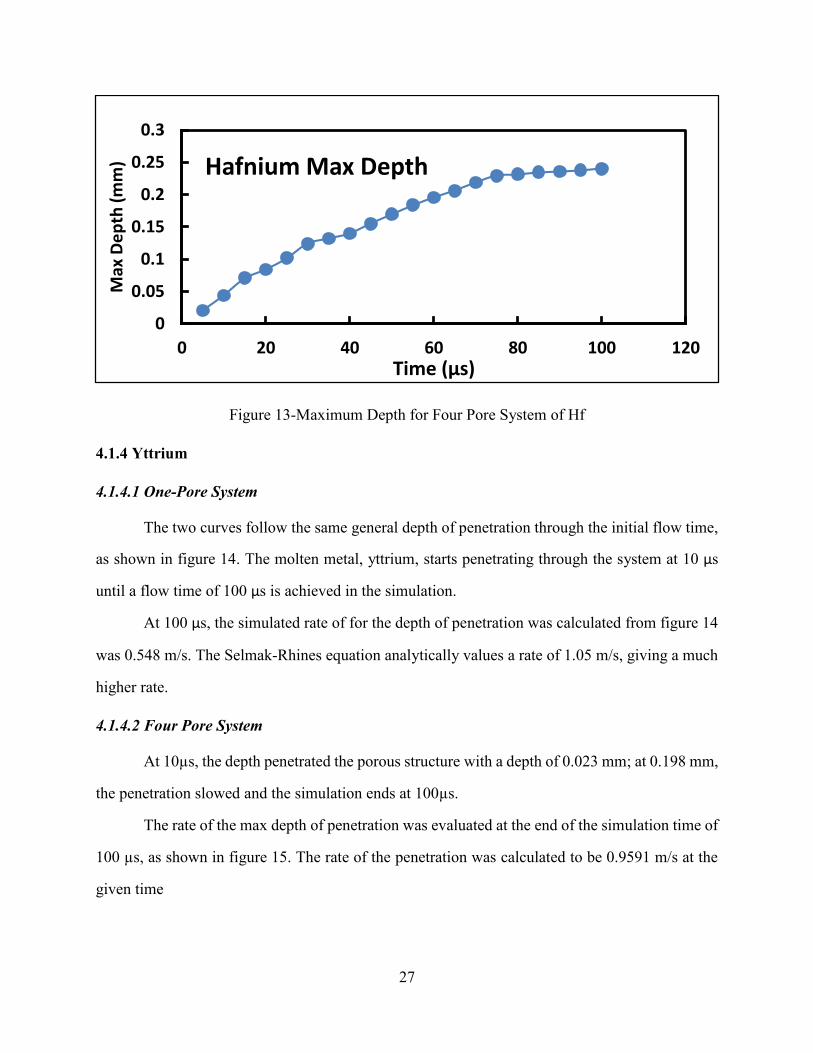
4.1.3.2 Four Pore System
The penetration of the molten metal through the four pore system from 10 to 100 µs of
flow time, as shown in figure 13. The simulation calculates a maximum penetration of 0.24 mm at
the maximum flow time.
The rate of penetration at the maximum depth of penetration for the current system was
calculated from figure 13. The value of the rate of penetration calculates to 0.347 m/s and is one
of the lowest rates compared to the other liquids melting temperature at 100 µs.
Figure 12-Depth of Penetration of Hf at Melting Point.
0
0.05
0.1
0.15
0.2
0.25
0.3
0 20 40 60 80 100 120
De
pth
(m
m)
Time (µs)
Hafnium
Selmak-Rhines
CFD
27
Figure 13-Maximum Depth for Four Pore System of Hf
4.1.4 Yttrium
4.1.4.1 One-Pore System
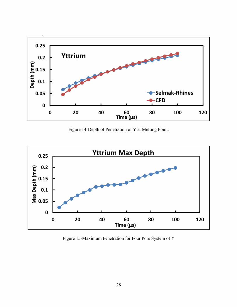
The two curves follow the same general depth of penetration through the initial flow time,
as shown in figure 14. The molten metal, yttrium, starts penetrating through the system at 10 µs
until a flow time of 100 µs is achieved in the simulation.
At 100 µs, the simulated rate of for the depth of penetration was calculated from figure 14
was 0.548 m/s. The Selmak-Rhines equation analytically values a rate of 1.05 m/s, giving a much
higher rate.
4.1.4.2 Four Pore System
At 10µs, the depth penetrated the porous structure with a depth of 0.023 mm; at 0.198 mm,
the penetration slowed and the simulation ends at 100µs.
The rate of the max depth of penetration was evaluated at the end of the simulation time of
100 µs, as shown in figure 15. The rate of the penetration was calculated to be 0.9591 m/s at the
given time
0
0.05
0.1
0.15
0.2
0.25
0.3
0 20 40 60 80 100 120
Max
De
pth
(m
m)
Time (µs)
Hafnium Max Depth
28
.
Figure 14-Depth of Penetration of Y at Melting Point.
Figure 15-Maximum Penetration for Four Pore System of Y
0
0.05
0.1
0.15
0.2
0.25
0 20 40 60 80 100 120
De
pth
(m
m)
Time (µs)
Yttrium
Selmak-RhinesCFD
0
0.05
0.1
0.15
0.2
0.25
0 20 40 60 80 100 120
Max
De
pth
(m
m)
Time (µs)
Yttrium Max Depth

29
4.1.5 Samarium
4.1.5.1 One Pore System
The depth of penetration at the maximum point in time of 100 µs, as shown in figure 16.
The recorded depth of penetration was 0.210 mm according to the CFD and 0.216 mm for the
Selmak-Rhines equation.
A rate of penetration was calculated using the data from the graph above and is evaluated
at the maximum flow time of this simulation. From the CFD data, a rate of 1.12 m/s was
determined while the Selmak-Rhines equation predicted a value of1.08 m/s.
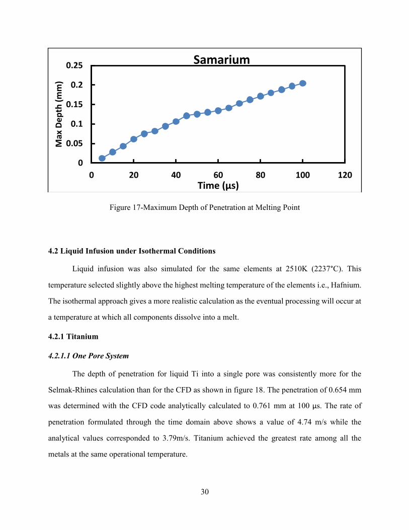
4.1.5.2 Four Pore System
The maximum depth of penetration for the Samarium system at its melting point was
determined to be 0.204 mm at the max time of 100 µs. The rate is determined with the CFD was
calculated at 1.14 m/s.
Figure 16-Depth of Penetration of Sm at Melting Point.
0
0.05
0.1
0.15
0.2
0.25
0 20 40 60 80 100 120
De
pth
(m
m)
Time (µs)
Samarium
Selmak-Rhines
CFD
30
Figure 17-Maximum Depth of Penetration at Melting Point
4.2 Liquid Infusion under Isothermal Conditions
Liquid infusion was also simulated for the same elements at 2510K (2237°C). This
temperature selected slightly above the highest melting temperature of the elements i.e., Hafnium.
The isothermal approach gives a more realistic calculation as the eventual processing will occur at
a temperature at which all components dissolve into a melt.
4.2.1 Titanium
4.2.1.1 One Pore System
The depth of penetration for liquid Ti into a single pore was consistently more for the
Selmak-Rhines calculation than for the CFD as shown in figure 18. The penetration of 0.654 mm
was determined with the CFD code analytically calculated to 0.761 mm at 100 µs. The rate of
penetration formulated through the time domain above shows a value of 4.74 m/s while the
analytical values corresponded to 3.79m/s. Titanium achieved the greatest rate among all the
metals at the same operational temperature.
0
0.05
0.1
0.15
0.2
0.25
0 20 40 60 80 100 120
Max
De
pth
(m
m)
Time (µs)
Samarium

31
4.2.1.2 Four Pore System
For the four pore system, the depth of penetration was calculated at the temperature of
2510K and acquired value of 0.401 mm at the maximum flow time of 60 µs. At 100 μs, the rate of
penetration for Ti reached a value of 1.45 m/s which is the highest rate of all the metals considered.
Figure 18-Depth of Penetration of Ti at 2510K
Figure 19-Maximum Penetration of Ti at 2510K
0
0.2
0.4
0.6
0.8
0 20 40 60 80 100 120
De
pth
(m
m)
Time (µs)
Titanium at 2510K
Selmak-Rhines
CFD

32
4.2.2 Zirconium
4.2.2.1 One Pore System
The depth of penetration for Zr into a single pore recorded the highest depth of 0.354 mm
through the CFD simulation, as shown in figure 20. The analytical solution calculated a value of
0.357 mm which gave a good convergence in the comparison. At 100 μs, the rate of penetration
for Zr valued at 1.54 m/s while the Selmak-Rhines calculation corresponded to 1.79 m/s.
4.2.2.2 Four Pore System
For the four pore system, the maximum depth of penetration increases as time increases
from 10 μs to 100 μs giving a maximum value of 0.338 mm. At 100 μs, a rate of penetration,
calculated a value of 1.34 m/s at 100 µs, shown in figure 21. This rate doubled compared to Zr at
its melting point of 2128K.
Figure 20-Maximum Depth of Penetration at 2510K
0
0.1
0.2
0.3
0.4
0 20 40 60 80 100 120
De
pth
(m
m)
Time (µs)
Zirconium at 2510K
Selmak-Rhines
CFD

33
Figure 21-Maximum Depth of Penetration at 2510K
4.2.3 Hafnium
4.2.3.1 One Pore System
The depth of penetration of hafnium measures a distance of 0.279 mm while the Selmak-
Rhines calculation predicted a depth of 0.282 mm at the maximum flow time of 100µs, as shown
in figure 22. At 100 µs, the rate of liquid hafnium was valued at 1.15m/s while, analytically,
Selmak-Rhines predicts a value of 1.40m/s.
4.2.3.2 Four Pore System
The four pore system had the depth of penetration of liquid hafnium at 2510K was valued
at 0.24 mm, as shown below in figure 23. At 100 μs, a rate of penetration was determined at a
value of 0.347 m/s. This value was near the rate at melting temperature because the operating
temperature was 10K greater than its melting point.
0
0.1
0.2
0.3
0.4
0 20 40 60 80 100 120
Max
De
pth
(m
m)
Time (µs)
Zirconium at 2510K

34
Figure 22-Depth of Penetration of Hf at 2510K
Figure 23-Maximum Depth of Hf at 2510K
0
0.05
0.1
0.15
0.2
0.25
0.3
0 20 40 60 80 100 120
De
pth
(m
m)
Time (µs)
Hafnium at 2510K
Selmak-Rhines
CFD
0
0.05
0.1
0.15
0.2
0.25
0.3
0 20 40 60 80 100 120
Max
De
pth
(m
m)
Time (µs)
Hafnium at 2510K

35
4.2.4 Yttrium
4.2.4.1 One Pore System
The depth of penetration of yttrium into a single pore measured a maximum depth of 0.486
mm for the CFD and 0.585 mm for the analytical solution, shown in figure 24. At 100 μs, the rate
of penetration of the fluid at an isothermal temperature of 2510K was calculated at 2.93m/s from
Selmak-Rhines analytical solution and 0.65 m/s from the CFD.
4.2.4.2 Four Pore System
The maximum depth of penetration for liquid yttrium at an isothermal temperature of
2510K was calculated at 80 µs was 0.39 mm, as shown in figure 25. At 80 μs, a rate of penetration
reached 1.26m/s for Y.
Figure 24-Depth of Penetration of Y at 2510K
0
0.1
0.2
0.3
0.4
0.5
0.6
0.7
0 20 40 60 80 100 120
De
pth
(m
m)
Time (µs)
Yttrium
Selmak-Rhines
CFD

36
Figure 25-Maximum Penetration of Y at 2510K
4.3 Elements through Temperature Range
The liquid elements were simulated through a temperature range from 1700°C to 1900°C
for titanium and yttrium; at the same time domain, hafnium and zirconium were simulated from
2250°C to 2450°C. A rate of penetration was investigated to grasp the effects of temperature on
these metals at a temperature greater than their molten states. Since the depth of penetration of the
liquid elements are simulated at similar temperatures, it gives a “real-world” prediction of infusion.
4.3.1 Titanium and Yttrium
The rate of penetration of the liquid metals were recorded as temperature increases from
1700°C to 1900°C, shown in figure 26. The comparison with Selmak-Rhines equation was also
calculated to see if the relationship shares the same trend.
0
0.1
0.2
0.3
0.4
0.5
0 20 40 60 80 100
Max
De
pth
(m
m)
Time (µs)
Yttrium at 2510K
Y Isothermal Max…

37
Figure 26-Rate of Penetration from 1700°C to 1900°C for Ti and Y
A common trend to notice was that both molten elements increase their rate of penetration
as temperature increases. This was lead back to the ratio of surface tension to viscosity and that
ratio increases faster with yttrium overcoming titanium after 1800°C according to Selmak-Rhines.
The CFD follows the same curve as the analytical solution, but yttrium was constantly at a higher
rate than titanium.
4.3.2 Hafnium and Zirconium
The rate of penetration of these liquid metals were evaluated as the temperature increased
from 2250°C to 2450°C, as shown in figure 27. The comparison with Selmak-Rhines equation was
also calculated to show a relationship between the two trends.
0
0.5
1
1.5
2
2.5
1650 1700 1750 1800 1850 1900 1950
dh
/dt
(m/s
)
Temperature (°C)
Rate of Ti and Y at 100 µs
Y Rate
Y Rate CFD
Ti Rate
Ti Rate CFD

38
Figure 27-Rate of Penetration from 2250C to 2450C for Ti and Y.
The liquid Zr consistently has a greater rate than the liquid Hf, though, both metals increase
their penetration rate as temperature increases. The ratio of surface tension to viscosity plays a
huge role in determining infusion and that ratio increases faster for liquid Zr than Hf which
analytically comes to the same conclusion. The CFD is slightly lower in rate compared to Selmak-
Rhines, but follow the same trend compared to the metals.

39
Chapter 5: Discussion
5.1 Surface Tension – Viscosity Ratio
From the results section in the previous
chapter, one of the consistent observations was
the depth relying on the parameter of surface
tension to viscosity ratio. Based on the overall
units of the ratio, this parameter gave a
characteristic velocity term. When comparing
the liquid elements at their respective melting
temperature and at the isothermal temperature,
one can see the effects of the ratio on the infusion depth from the CFD data, as shown in figure 28
and 29. The comparison of the ratio between the two temperatures simulated shows the vast
increased values which affect the depth of infusion, as presented in table 2. The depth of
penetration in the one pore system shows that Ti, Hf, and Zr have relatively the same range of
infusion while Y and Sm lag behind the curve. This changes as the temperature of infusion depth
was increased to 2510K as yttrium’s depth became the second highest recorded.
Figure 28- Depth of Penetration of Elements at Melting Point
Table 2-Surface Tension - Viscosity Ratio at
Melting Point and 2510K

40
Figure 29- Depth of Penetration of Elements at 2510K
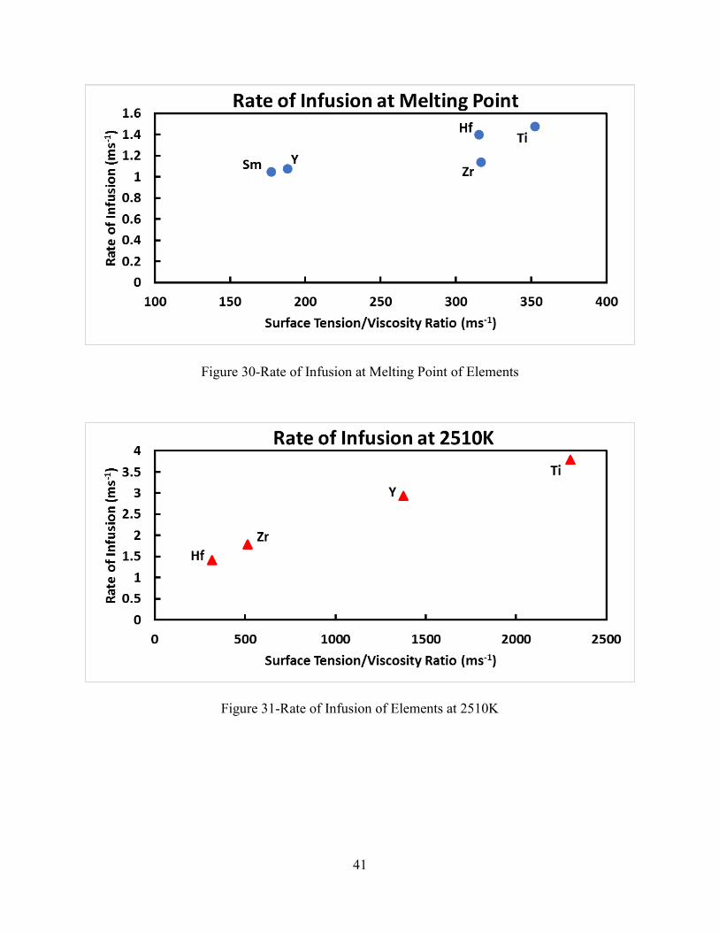
5.2 Rate of Infusion
Compared at 100 μs, the rate of
penetration follows the same trend as the depth
with the difference in operating temperatures,
as shown in table 3. The rates increased with
increased temperature allowing the metal to
infuse into the pore more rapidly. The Selmak-
Rhines equation heavily relied on the ratio,
explained above, to predict a rate as the metal
infused into the pore from melting temperature of the respecting metals to the isothermal
temperature of 2510K, shown in figure 30 and 31. As the temperature increases, titanium and
yttrium increase their overall rate of penetration drastically because the element’s viscosity
decrease at a faster proportion to temperature than the surface tension.
Table 3-Rate of Infusion at Melting Point and
2510K.
41
Figure 30-Rate of Infusion at Melting Point of Elements
Figure 31-Rate of Infusion of Elements at 2510K

42
Chapter 6: Conclusion
A depth and rate of penetration for the liquid infusion into a packed bed was simulated
with computational fluid dynamic software (i.e. ANSYS FLUENT) and an analytical calculation
developed by Selmak-Rhines. The infusion was assumed to occur without any reaction between
the liquid metal and pore with consideration of only the momentum balance equation incorporating
the accumulation of momentum and forces for a liquid into a capillary. The liquid element (e.g.
yttrium, titanium, hafnium, zirconium, and samarium) was predicted at their respected melting
temperatures giving titanium with the highest rate at 1.48m/s theoretical (1.14m/s computed by
CFD) and yttrium at the lowest rate at 1.04m/s theoretical (0.548m/s computed by CFD). At the
isothermal temperature of 2510K (2237°C), though, the metals whose melting temperatures are
further from the operational temperature experience an increase rate in penetration. This is due to
the surface tension-to-viscosity ratio in each of the elements properties; as temperature increases,
viscosity decreases at a faster degree than surface tension making the penetration easier through
the pore. For example, the surface tension-to-viscosity value for titanium at its melting point was
calculated as 352.26 ms-1 while at 2510K was 2301.4 ms-1; this gave a 6.5 times increase from
melting to isothermal temperature. At each melting temperature, titanium was the superior element
while yttrium lagging behind in depth of penetration compared with the other metals investigated.
When the temperature increases to 2510K, titanium still maintains its advantage in depth of
penetration. However, yttrium’s depth of penetration increased significantly and should be
considered in infusing the liquid metal into a packed bed at that operating temperature for future
projects.

43
REFERENCES
[1] W. B. Johnson, A. S. Nagelberg and E. Breval, "Kinetics of Formation of a Platelet-
Reinforced Ceramic Composite Prepared by the Directed Reation of Zirconium with Boron
Carbide," Journal of American Ceramics, pp. 2093-2101, 1991.
[2] M. J. Gasch, D. T. Ellerby and S. M. Johnson, "Ultra High Temperature Ceramic
Composites," in Handbook of Ceramic Composites, 2005, pp. 197-224.
[3] K. A. Semlak and F. N. Rhines, "The Rate of Infiltration of Metals," Transactions of The
Metallurical Socitry of AIME, pp. 325-331, 1958.
[4] D. C. Halverson, A. J. Pyzik, I. A. Aksay and W. E. Snowden, "Processing of Boron
Carbide-Aluminum Composites," Journal American Ceramics Society, pp. 775-780, 1989.
[5] J. R. Ligenza and R. B. Bernstein, "The Rate of Rise of Liquids in Fine Vertical
Capillaries," 1951.
[6] G. P. Martins, D. L. Olson and G. R. Edwards, "Modeling of Infiltration Kinetics for
Liquid Metal Processing of Composites," Metallurgical Transactions, pp. 95-101, 1988.
[7] F. Delanny, L. Froyen and A. Deruyttere, "Review: The Wetting of Solids by Molten
Metals and its Relation to the Preparation of Metal-Matrix Composites," Journal of
Material Science, pp. 1-16, 1987.
[8] I. ANSYS, ANSYS FLUENT: Theory Guide, 2009.
[9] J. U. Brackbill, D. B. Kothe and C. Zemach, "A Continuum Method for Modeling Surface
Tension," Journal of Computational Physics, pp. 335-354, 1992.
[10] L. Trefethen, "Surface Tension in Fluid Mechanics," Chicago, 1969.
[11] F. Aqra and A. Ayyad, "Surface Tension, Surface Energy, and Crystal-Melt Interfacial
Energy of Metals," Current Applied Physics, vol. 12, pp. 31-35, 2012.
[12] A. W. Peterson, H. Kedesdy, P. H. Keck and E. Schwarz, "Surface Tension of Titanium,
Zirconium, and Hafnium," Journal of Applied Physics, pp. 213-216, 1958.
[13] P. F. Paradis, T. Ishikawa and S. Yoda, "Non-Contact Measurements of Surface Tension
and Viscosity of Niobium, Zirconium, and Titanium Using an Electrostatic Levitaion
Furance," International Journal of Thermophyics, pp. 825-842, 2002.
[14] F. Aqra and A. Ayyad, "Surface Energies of Metals in Both Liquid and Solid States,"
Applied Surface Science, vol. 257, pp. 6372-6379, 2011.
[15] R. M. Digilov, "Solid-Liquid Infacial Tension in Metals: Correlation with the Melting
Point," Physica B, vol. 352, pp. 53-60, 2004.
[16] E. D. Hondros, "Interfacial Engergies and Composition in Solids," in TMS-AIME, Niagara
Falls, 1976.
[17] W. Tian, "Wetting and Joining of Structural Ceramic Components," in MAX Phases and
Ultra-High Temperature Ceramics for Extreme Environments, Hershey, IGI Global, 2013,
pp. 461-472.
[18] R. G. Gilliland, "Investigation of the Wettability of Various Pure Metals and Alloys on
Beryllium," 1963.

44
[19] D. E. Sullivan, "Surface Tension and Contact Angle of a Liquid-Soild Interface," The
Journal of Chemical Physics, vol. 74, no. 4, pp. 2604-2615, 1981.
[20] E. Saiz and A. P. Tomsia, "Kinetics of High-Temperature Spreading," Current Opinion in
Solid State and Materials Science, vol. 9, pp. 167-173, 2005.
[21] E. Saiz, C. W. Hwang, K. Suganuma and A. P. Tomsia, "Spreading of Sn-Ag Solders on
FeNi Alloys," Acta Materialia, vol. 51, pp. 3185-3197, 2003.
[22] P. F. Paradis, T. Ishikawa, T. Itami and S. Yoda, "Non-Contact Thermophsical Property
Measurements of Refractory Metals Using an Electrostatic Levitator," Measurement
Science and Technology, vol. 16, pp. 443-451, 2005.
[23] O. K. Echendu, E. C. Mbamala and B. C. Anusionwu, "Theoretical Investigation of the
Viscosity of Some Liquid Metals and Alloys," Physics and Chemistry of Liquids, vol. 49,
no. 2, pp. 247-258, 2011.
[24] P. F. Paradis and W.-K. Rhim, "Non-Contact Measurements of Thermophysical Properties
of Titanium at High Temperature," Jet Propulsion Laboratory, Pasadena.
[25] P. F. Paradis, T. Ishikawa and S. Yoda, "Non-Contact Measurements of Surface Tension
and Viscosity of Niobium, Zirconium, and Titanium Using an Electrostatic Levitation
Furance," International Journal of Thermophysics, vol. 23, no. 3, pp. 825-842, 2002.
[26] P. F. Paradis and W. K. Rhim, "Thermophysical Properties of Zirconium Measured Using
Electrostatic Levitation".
[27] P. F. Paradis, T. Ishikawa and N. Koike, "Thermophysical Properties of Molten Yttrium
Measured by Non-Contact Techniques," Microgravity Science Technology, vol. 21, pp.
113-118, 2009.
[28] P. F. Paradis, T. Ishikawa and S. Yoda, "Non-Contact Measurements of the
Thermophysical Properties of Hafnium-3% mass % Zirconium at High Temperature,"
International Journal of Thermophysics , vol. 24, no. 1, pp. 239-258, 2003.
[29] B. J. Keene, "Review of Data of Surface Tension of Pure Metals," in International
Materials Reviews, London, The Institute of Materials, 1993, pp. 157-192.
[30] T. Iida, R. Guthrie, M. Isac and N. Tripathi, "Accurate Predictions for the Viscosities of
Several Liquid Transition Metals, Plus Barium and Strontium," Metallurgical and
Materials Transactions, pp. 403-416, 2006.
[31] S. V. Strankus and P. V. Tyagel'skii, "Electronic Phase Transition in Liquid Samarium,"
Thermophysical Properties of Materials , pp. 660-664, 2001.

45
Vita
Arturo Medina, son of Arturo Rolando Medina and Margarita Medina, was born on January
15, 1988 in El Paso, TX, USA. He completed his high school education from Bel Air High School
in 2006 and then joined El Paso Community College (EPCC) in 2007 later joining The University
of Texas at El Paso in the summer of 2008 to pursue his Bachelor of Science in Mechanical
Engineering (BSME). During his last year as an undergraduate, he became an Engineering
Ambassador promoting the importance of engineering to local schools throughout the El Paso area.
In that same year, he helped conduct the design, fabrication, and testing of HAYNES 230 nozzles
for his senior project in the fall of 2011. After completion of his BSME, his joined UTEP in the
fall of 2012 to pursue his Master of Science in Mechanical Engineering. During those years, he
worked as a Graduate Research Assistant under the supervision of Dr. Arturo Bronson. His studies
consisted on the effects of ultra-high temperature on molten liquid elements (e.g. titanium,
zirconium, hafnium, yttrium, and samarium). He has also been participated in two internships in
the summers of 2013 and 2014 at Kirtland Air Force Research Laboratory in Albuquerque, NM.
His work consisted in designing circuit boards for signal processing and manipulation of sensors
into a data acquisition board in 2013. In summer 2014, he lead and redesigned and experiment to
study the flow effects of a pulse tube from a pulse tube cryocooler in an enclosed area. After his
graduation, he will pursue a career with the Federal Aviation Administration (FAA) as a
mechanical engineer.
Permanent address: 828 Lomaland Dr.
El Paso, Texas, 79907
This thesis/dissertation was typed by Arturo Medina.
Top Related