


Languages
Pages
Legal

04/20/23
Signals & systemsCh.3 Fourier Transform of
Signals and LTI System
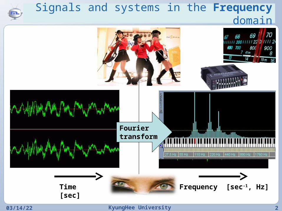
Signals and systems in the Frequency domain
04/20/23 KyungHee University 2
Time [sec]
Frequency [sec-1, Hz]
Fourier transform
04/20/23 KyungHee University 3
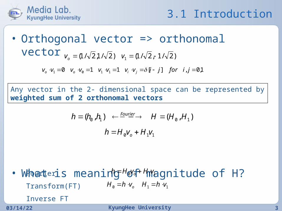
3.1 Introduction
• Orthogonal vector => orthonomal vector
• What is meaning of magnitude of H?
)2/1,2/1()2/1,2/1( 1 vvo
1,0,][110 1101 jiforjivvvvvvvv jioo
),(),( 1010 HHHhhh Fourier
110 vHvHh o
110 vHvHh o
110 vhHvhH o
Any vector in the 2- dimensional space can be represented by weighted sum of 2 orthonomal vectors
Fourier Transform(FT)
Inverse FT
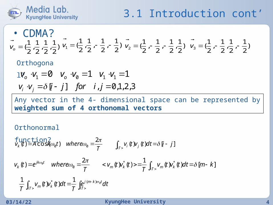
3.1 Introduction cont’
• CDMA?
04/20/23 KyungHee University 4
1 1 1 1( , , , )2 2 2 2ov
Orthogonal
? 1 0 1 10 1 1o ov v v v v v
[ ] , 0,1,2,3i jv v i j for i j
Any vector in the 4- dimensional space can be represented by weighted sum of 4 orthonomal vectors
Orthonormal
function?][)()(
2)cos()( 00 jidttvtv
TwheretkAtv
T jik
][)()(1
)()(2
)( **0
0 kmdttvtvT
tvtvT
whereetvT kmkm
tjkk
T
tkmj
T km dteT
dttvtvT
0)(* 1)()(
1
1
1 1 1 1( , , , )2 2 2 2
v
2
1 1 1 1( , , , )2 2 2 2
v
3
1 1 1 1( , , , )2 2 2 2
v
3.1 Introduction cont’
• Fourier Series (FS)
04/20/23 KyungHee University 5
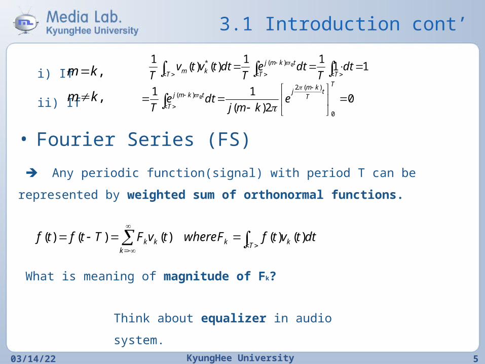
i) If
ii) If ,km
1111
)()(1
0)(*
TT
tkmj
T km dtT
dteT
dttvtvT
02)(
11
0
)(2)( 0
T
tT
kmj
T
tkmj ekmj
dteT
,km
Any periodic function(signal) with period T can be represented by
weighted sum of orthonormal functions.
T kkk
kk dttvtfFwheretvFTtftf )()()()()(
What is meaning of magnitude of Fk?
Think about equalizer in audio
system.
3.2 Complex Sinusoids and Frequency Response of LTI
Systems
04/20/23 KyungHee University 6
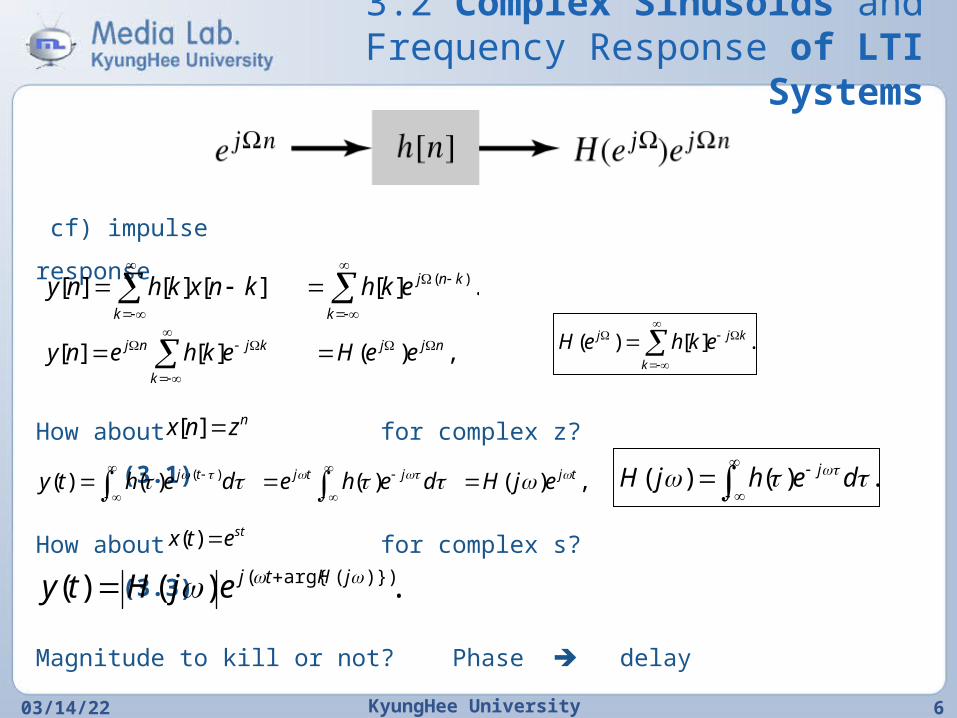
cf) impulse response
.][ ][][][ )(
k
knj
k
ekhknxkhny
,)( ][][ njj
k
kjnj eeHekheny
.][)(
k
kjj ekheH
How about for complex z? (3.1) nznx ][
,)( )( )()( )( tjjtjtj ejHdehedehty
.)()(
dehjH j
How about for complex s? (3.3) stetx )(
.)()( )})(arg{( jHtjejHty
Magnitude to kill or not? Phase delay
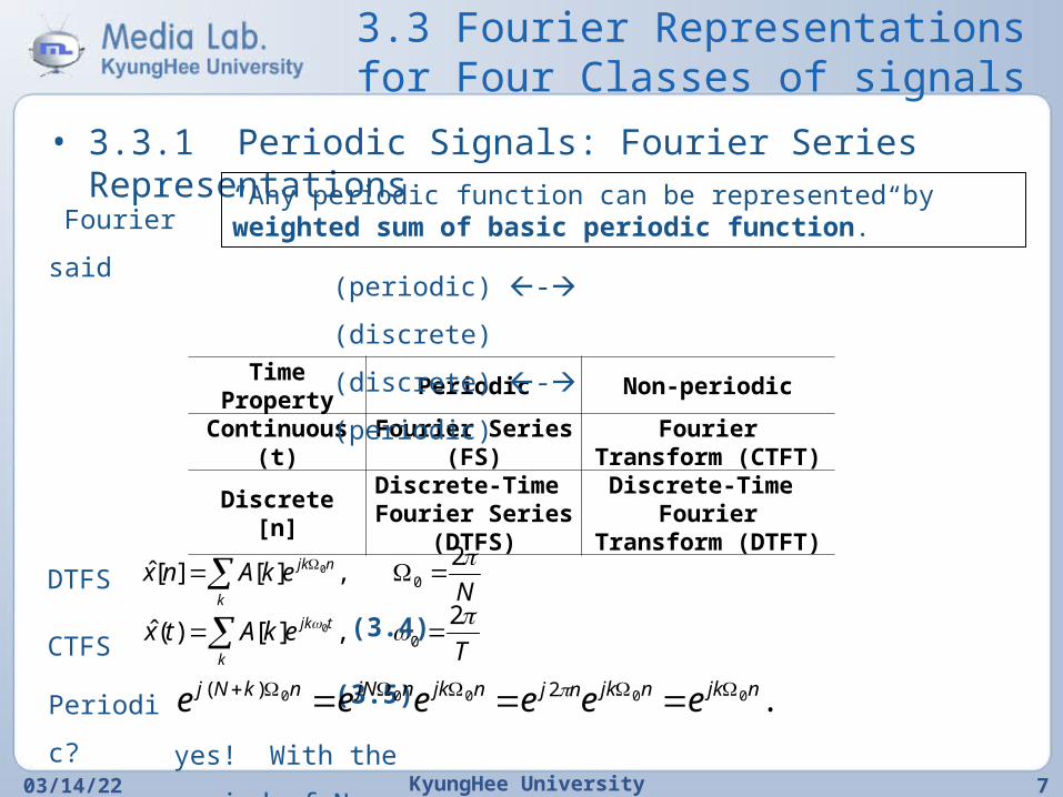
3.3 Fourier Representations for Four Classes of signals
• 3.3.1 Periodic Signals: Fourier Series Representations
04/20/23 KyungHee University 7
“Any periodic function can be represented by weighted sum of basic periodic function.” Fourier
said
Time Property
Periodic Non-periodic
Continuous (t)
Fourier Series (FS)
Fourier Transform (CTFT)
Discrete [n]Discrete-Time Fourier Series
(DTFS)
Discrete-Time Fourier
Transform (DTFT)
(periodic) -
(discrete)
(discrete) -
(periodic)
NekAnx
k
njk 2,][][ˆ 0
0
TekAtx
k
tjk 2,][)(ˆ 0
0 CTFS (3.5)
DTFS (3.4)
. 00000 2)( njknjknjnjknjNnkNj eeeeee Periodic
?
yes! With the period of
N
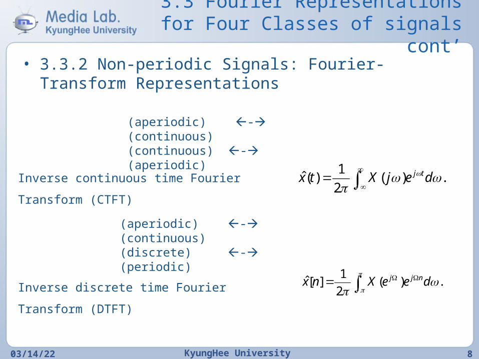
3.3 Fourier Representations for Four Classes of signals cont’
• 3.3.2 Non-periodic Signals: Fourier-Transform Representations
04/20/23 KyungHee University 8
(aperiodic) - (continuous)(continuous) - (aperiodic)
Inverse continuous time Fourier Transform
(CTFT)
.)(2
1)(ˆ
dejXtx tj
(aperiodic) - (continuous)(discrete) - (periodic)
Inverse discrete time Fourier Transform
(DTFT)
.)(2
1][ˆ
deeXnx njj
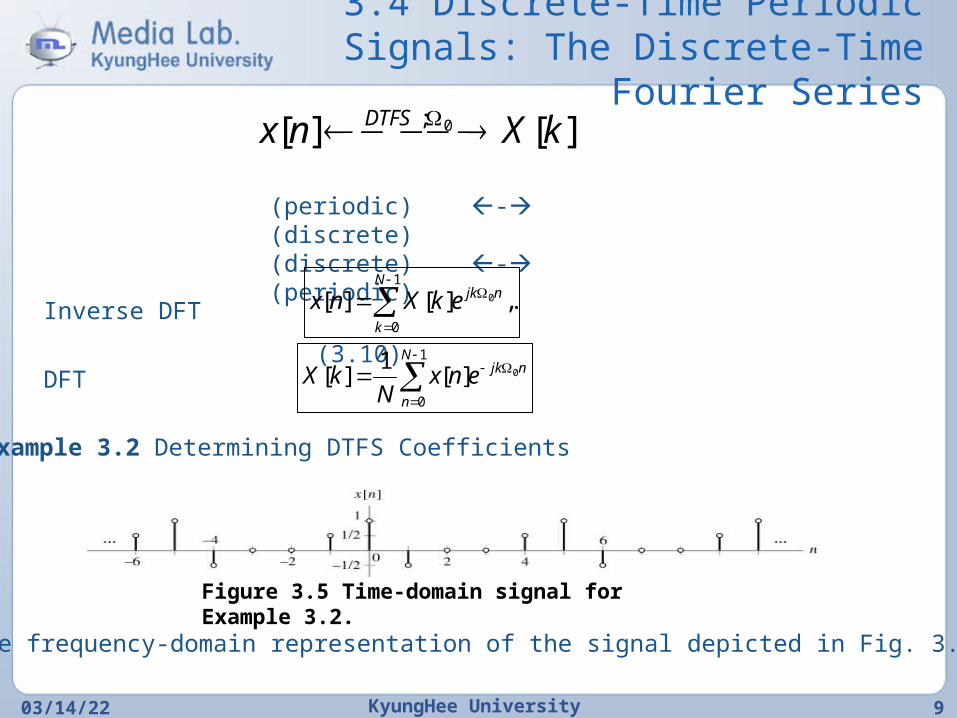
3.4 Discrete-Time Periodic Signals: The Discrete-Time
Fourier Series
04/20/23 KyungHee University 9
][][ 0; kXnx DTFS
(periodic) - (discrete)(discrete) - (periodic)
Inverse DFT (3.10)
DFT
.,][][1
0
0
N
k
njkekXnx
1
0
0][1
][N
n
njkenxN
kX
Example 3.2 Determining DTFS Coefficients
Find the frequency-domain representation of the signal depicted in Fig. 3.5
Figure 3.5 Time-domain signal for Example 3.2.
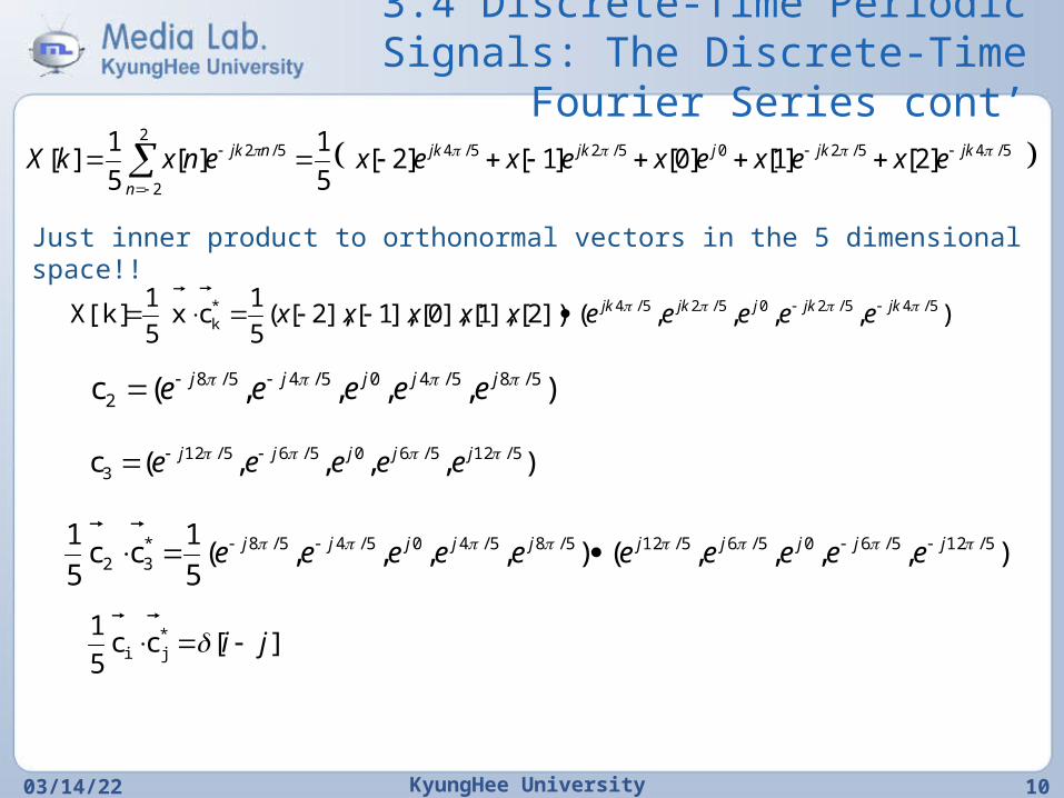
3.4 Discrete-Time Periodic Signals: The Discrete-Time
Fourier Series cont’
04/20/23 KyungHee University 10
5/45/205/25/42
2
5/2 ]2[]1[]0[]1[]2[5
1][
5
1][ jkjkjjkjk
n
njk exexexexexenxkX
Just inner product to orthonormal vectors in the 5 dimensional space!!
),,,,(])2[],1[],0[],1[],2[(5
1 cx
5
1 X[k] 5/45/205/25/4*
k jkjkjjkjk eeeeexxxxx
),,,,(c 5/85/405/45/82
jjjjj eeeee
),,,,( c 5/125/605/65/123
jjjjj eeeee
),,,,(),,,,(5
1 cc
5
1 5/125/605/65/125/85/405/45/8*
32 jjjjjjjjjj eeeeeeeeee
][cc 5
1 *
ji ji
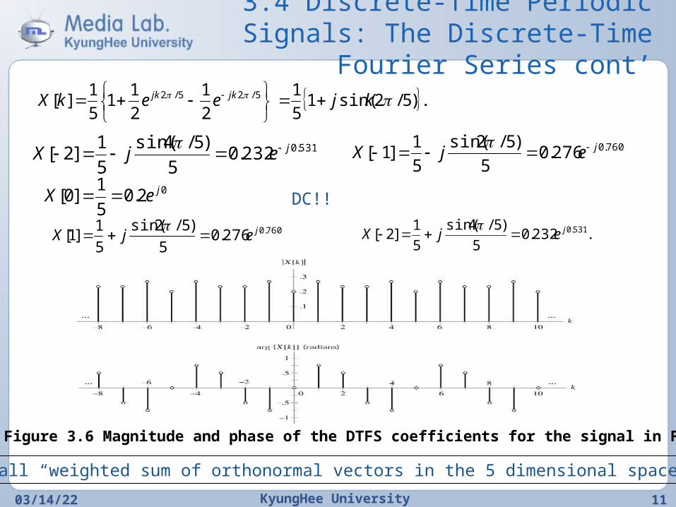
3.4 Discrete-Time Periodic Signals: The Discrete-Time
Fourier Series cont’
04/20/23 KyungHee University 11
.)5/2sin(15
1
2
1
2
11
5
1][ 5/25/2 kjeekX jkjk
531.0232.05
)5/4sin(
5
1]2[ jejX
760.0276.05
)5/2sin(
5
1]1[ jejX
02.05
1]0[ jeX DC!!
760.0276.05
)5/2sin(
5
1]1[ jejX
.232.0
5
)5/4sin(
5
1]2[ 531.0jejX
Figure 3.6 Magnitude and phase of the DTFS coefficients for the signal in Fig. 3.5.
Recall “weighted sum of orthonormal vectors in the 5 dimensional space”
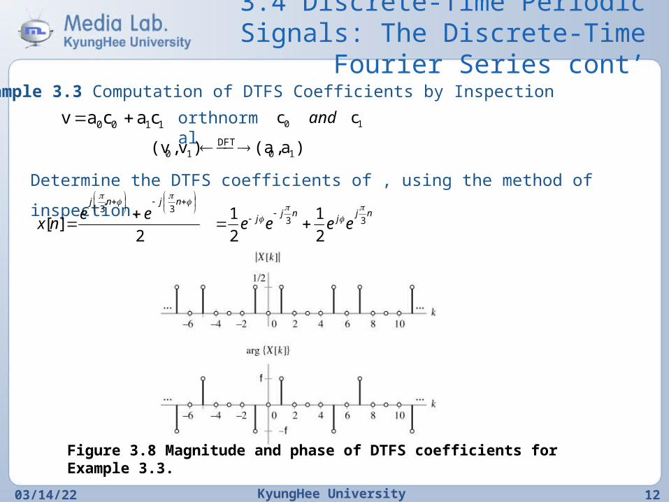
3.4 Discrete-Time Periodic Signals: The Discrete-Time
Fourier Series cont’
04/20/23 KyungHee University 12
Example 3.3 Computation of DTFS Coefficients by Inspection
11 00 cacav
1 0 cc
andorthnormal
)a,(a)v,(v 10DFT
10
Determine the DTFS coefficients of , using the method of
inspection. njj
njj
njnj
eeeeee
nx 3333
2
1
2
1
2 ][
Figure 3.8 Magnitude and phase of DTFS coefficients for Example 3.3.
3.4 Discrete-Time Periodic Signals: The Discrete-Time
Fourier Series cont’
04/20/23 KyungHee University 13
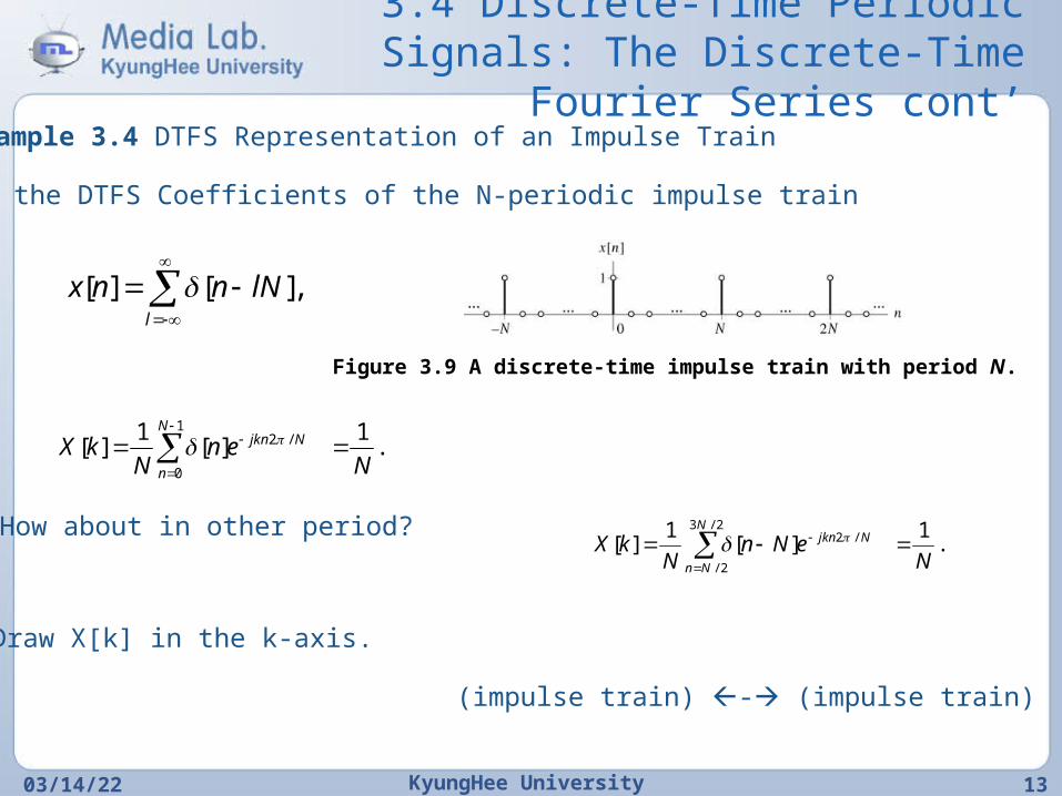
Example 3.4 DTFS Representation of an Impulse Train
Find the DTFS Coefficients of the N-periodic impulse train
,][][
l
lNnnx
Figure 3.9 A discrete-time impulse train with period N.
.1
][1
][1
0
/2
Nen
NkX
N
n
Njkn
How about in other period?
Draw X[k] in the k-axis.
.`1
][1
][2/3
2/
/2
NeNn
NkX
N
Nn
Njkn
(impulse train) - (impulse train)
3.4 Discrete-Time Periodic Signals: The Discrete-Time
Fourier Series cont’
04/20/23 KyungHee University 14
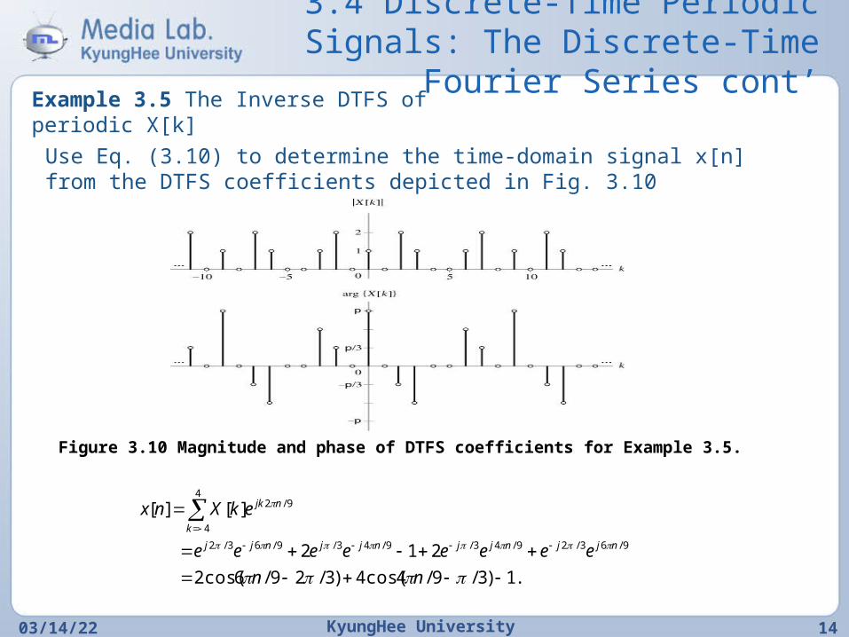
Example 3.5 The Inverse DTFS of periodic X[k]
Use Eq. (3.10) to determine the time-domain signal x[n] from the DTFS coefficients depicted in Fig. 3.10
Figure 3.10 Magnitude and phase of DTFS coefficients for Example 3.5.
.1)3/9/4cos(4)3/29/6cos(2
212
][ ][
9/63/29/43/9/43/9/63/2
4
4
9/2
nn
eeeeeeee
ekXnx
njjnjjnjjnjj
k
njk
3.4 Discrete-Time Periodic Signals: The Discrete-Time
Fourier Series cont’
04/20/23 KyungHee University 15
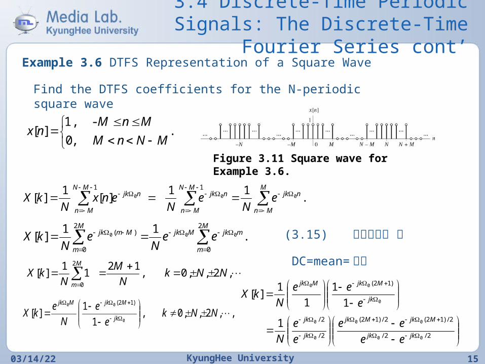
Example 3.6 DTFS Representation of a Square Wave
Find the DTFS coefficients for the N-periodic square wave
. ,0
- 1,][
MNnM
MnMnx
Figure 3.11 Square wave for Example 3.6.
.1
1
][1
][ 000
11
M
Mn
njkMN
Mn
njkMN
Mn
njk eN
eN
enxN
kX
.1
1
][2
0
2
0
)( 000
M
m
mjkMjkM
m
Mmjk eeN
eN
kX (3.15) 등비수열의 합
,2,0, ,12
11
][2
0
NNkN
M
NkX
M
m
DC=mean= 평균
,,2,0, ,1
1][
0
00 )12(
NNke
e
N
ekX
jk
MjkMjk
1
1
1
1
1][
2/2/
2/)12(2/)12(
2/
2/
)12(
00
00
0
0
0
00
jkjk
MjkMjk
jk
jk
jk
MjkMjk
ee
ee
e
e
N
e
ee
NkX
3.4 Discrete-Time Periodic Signals: The Discrete-Time
Fourier Series cont’
04/20/23 KyungHee University 16
.,2,0, ,)2/sin(
)2/)12(sin(1][
0
0 NNkk
Mk
NkX
.
,2,0, ,/)12(
,2,0, ,)/sin(
)/)12(sin(1
][
NNkNM
NNkNk
NMk
NkX
.12
)/sin(
)/)12(sin(1lim
,2,0, N
M
Nk
NMk
NNNk
DC, also
.)/sin(
)/)12(sin(1][
Nk
NMk
NkX
Then for all k.
M=0 (impulse train)
2M+1 = N? ?)/sin(
)sin(1][
Nk
k
NkX
(square) - (sinc)
3.4 Discrete-Time Periodic Signals: The Discrete-Time
Fourier Series cont’
04/20/23 KyungHee University 17
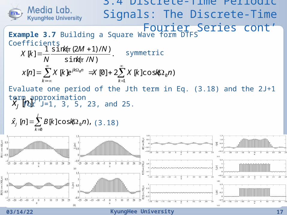
Example 3.7 Building a Square Wave form DTFS Coefficients
.)/sin(
)/)12(sin(1][
Nk
NMk
NkX
1
0 )cos(][2]0[][][ 0
kk
njk nkkXXekXnx
symmetric
Evaluate one period of the Jth term in Eq. (3.18) and the 2J+1 term approximation
][ˆ nxJ for J=1, 3, 5, 23, and 25.
,)cos(][][ˆ0
0
J
kJ nkkBnx (3.18)
3.4 Discrete-Time Periodic Signals: The Discrete-Time
Fourier Series cont’
04/20/23 KyungHee University 18
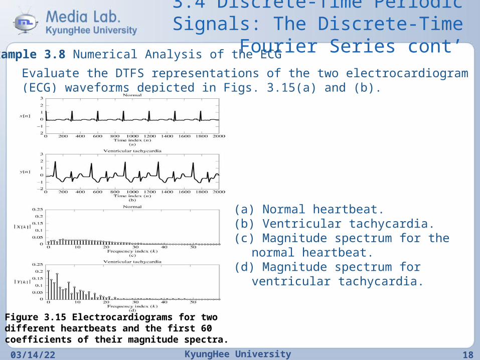
Example 3.8 Numerical Analysis of the ECG
Evaluate the DTFS representations of the two electrocardiogram (ECG) waveforms depicted in Figs. 3.15(a) and (b).
Figure 3.15 Electrocardiograms for two different heartbeats and the first 60 coefficients of their magnitude spectra.
(a) Normal heartbeat. (b) Ventricular tachycardia. (c) Magnitude spectrum for the
normal heartbeat. (d) Magnitude spectrum for
ventricular tachycardia.
3.5 Continuous-Time Periodic Signals: The Fourier Series
04/20/23 KyungHee University 19
Any periodic function can be represented by weighted sum of basic periodic functions.
(periodic) (discrete)(continuous) (aperiodic)
Inverse FT where (3.19) Recall “orthonormal”!!
.,][)( 0
k
tjkekXtx
T tjk dtetx
TkX
0
0)(1
][ FT (3.20)
3.5 Continuous-Time Periodic Signals: The Fourier Series cont’
04/20/23 KyungHee University 20
Example 3.9 Direct Calculation of FS CoefficientsDetermine the FS coefficients for the signal depicted in Fig. 3. 16.
)(tx
Solution :
24
1
)2(2
1
2
1
2
1][
420
)2(2
0
)2(2
0
2
jk
ee
jkdtedteekX tjktjktjkt
X[0]=?
FT
Figure 3.16 Time-domain signal for Example 3.9.
Figure 3.17 Magnitude and phase for Ex. 3.9.
3.5 Continuous-Time Periodic Signals: The Fourier Series cont’
04/20/23 KyungHee University 21
Example 3.10 FS Coefficients for an Impulse Train. Determine the FS
coefficients for the signal defined by
t
lttx )4()(
Solution :
6
2
)2/(2
2
)2/()2/( )4(4
1)(
4
1)(
4
1][ dtetdtetdtetxkX tjktjk
T
tjk
(impulse train) (impulse train)
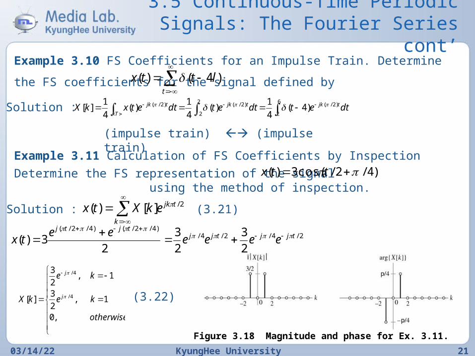
Example 3.11 Calculation of FS Coefficients by Inspection
Determine the FS representation of the signal using the method of inspection.
)4/2/cos(3)( ttx
Solution :
k
tjkekXtx 2/][)( (3.21)
2/4/2/4/)4/2/()4/2/(
2
3
2
3
23)( tjjtjj
tjtj
eeeeee
tx
otherwise
ke
ke
kX j
j
,0
1,2
3
1,2
3
][ 4/
4/
(3.22)
Figure 3.18 Magnitude and phase for Ex. 3.11.
3.5 Continuous-Time Periodic Signals: The Fourier Series cont’
04/20/23 KyungHee University 22
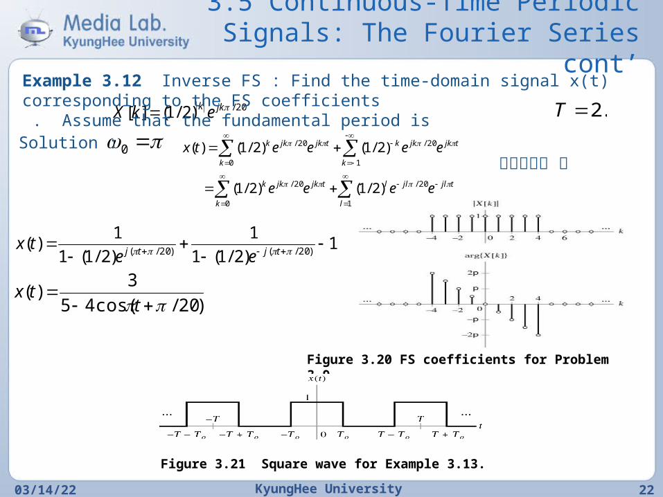
20/)2/1(][ jkk ekX .2T
Example 3.12 Inverse FS : Find the time-domain signal x(t) corresponding to the FS coefficients . Assume that the fundamental period is Solution : 0
1
20/
0
20/
1
20/
0
20/
)2/1()2/1(
)2/1()2/1()(
l
tjljll
k
tjkjkk
k
tjkjkk
k
tjkjkk
eeee
eeeetx
등비수열의 합
1)2/1(1
1
)2/1(1
1)(
)20/()20/(
tjtj ee
tx
)20/cos(45
3)(
ttx
Figure 3.20 FS coefficients for Problem 3.9.
Figure 3.21 Square wave for Example 3.13.
3.5 Continuous-Time Periodic Signals: The Fourier Series cont’
04/20/23 KyungHee University 23
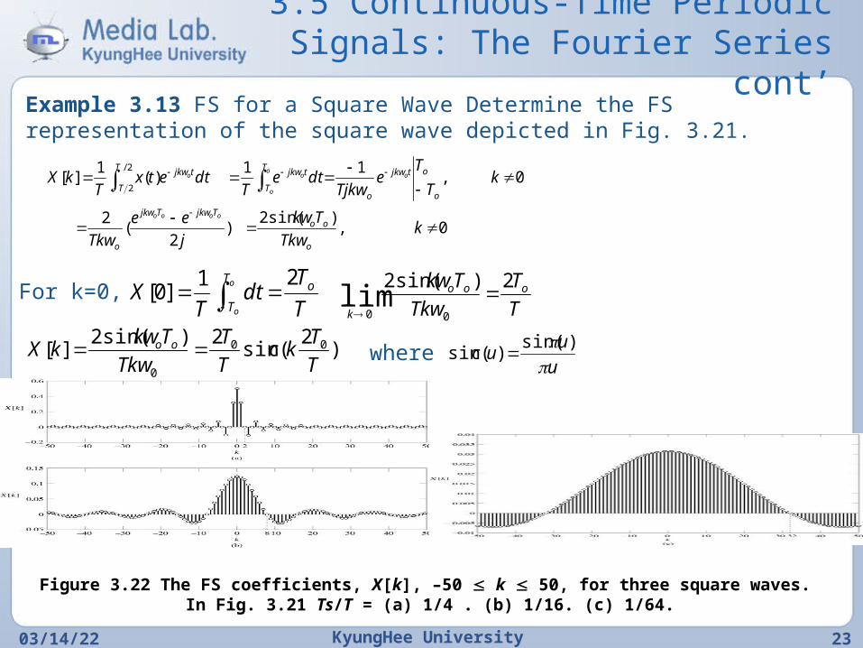
Example 3.13 FS for a Square Wave Determine the FS representation of the square wave depicted in Fig. 3.21.
0,)sin(2
)2
(2
0,11
)(1
][2/
2
kTkw
Tkw
j
ee
Tkw
kT
Te
Tjkwdte
Tdtetx
TkX
o
ooTjkwTjkw
o
o
otjkw
o
T
T
tjkwT
T
tjkw
oooo
oo
o
oo
For k=0, o
o
T
T
o
T
Tdt
TX
21]0[
T
T
Tkw
Tkw ooo
k
2)sin(2
00lim
)2
(sin2)sin(2
][ 00
0 T
Tkc
T
T
Tkw
TkwkX oo
u
uuc
)sin(
)(sin where
Figure 3.22 The FS coefficients, X[k], –50 k 50, for three square waves. In Fig. 3.21 Ts/T = (a) 1/4 . (b) 1/16. (c) 1/64.
3.5 Continuous-Time Periodic Signals: The Fourier Series cont’
04/20/23 KyungHee University 24
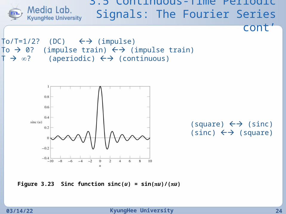
To/T=1/2? (DC) (impulse)To 0? (impulse train) (impulse train)T ? (aperiodic) (continuous)
Figure 3.23 Sinc function sinc(u) = sin(u)/(u)
(square) (sinc)(sinc) (square)
3.5 Continuous-Time Periodic Signals: The Fourier Series cont’
04/20/23 KyungHee University 25
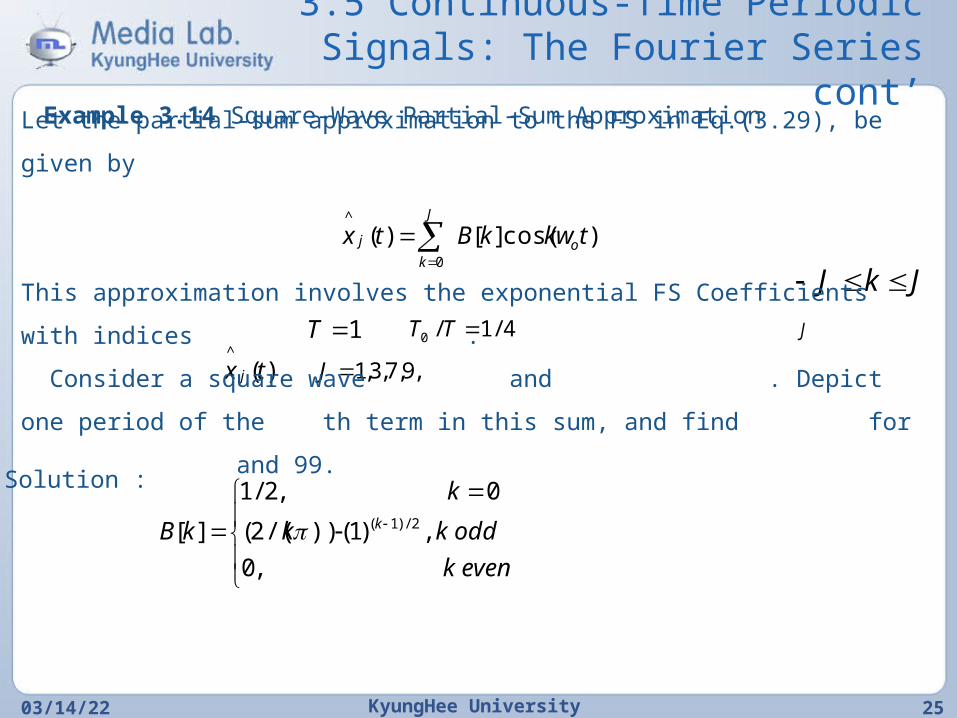
Example 3.14 Square-Wave Partial-Sum Approximation
)cos(][)(0
^
tkwkBtx o
J
k
j
JkJ
1T 4/1/0 TT J
)(^
tx j ,9,7,3,1J
Let the partial-sum approximation to the FS in Eq.(3.29), be given by
This approximation involves the exponential FS Coefficients with indices
.
Consider a square wave and . Depict one period of the
th term in this sum, and find for and 99.
Solution :
evenk
oddkk
k
kB k
,0
,)1))(/(2(
0,2/1
][ 2/)1(
3.6 Discrete-Time Non-periodic Signals : The Discrete-Time Fourier
Transform
04/20/23 KyungHee University 26
(discrete) (periodic)
deeXnx njnj )(
2
1][
n
njj enxeX ][)(
)(][ jDTFT eXnx
n
nx ][
n
nx2
][
(3.31)
(3.32)
3.6 Discrete-Time Non-periodic Signals : The Discrete-Time Fourier Transform cont’
04/20/23 KyungHee University 27
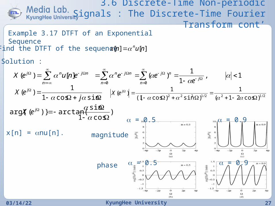
Example 3.17 DTFT of an Exponential Sequence
Find the DTFT of the sequence ][][ nunx n
Solution :
n n
njnnjnj eenueX0
][)( 1,1
1)(
0
j
n
nj
ee
sincos1
1)(
jeX j
2/122/1222 )cos21(
1
)sin)cos1((
1)(
jeX
)cos1
sinarctan()}(arg{
jeX
x[n] = nu[n]. magnitude
phase
= 0.5 = 0.9
= 0.5 = 0.9
3.6 Discrete-Time Non-periodic Signals : The Discrete-Time Fourier Transform
cont’
04/20/23 KyungHee University 28
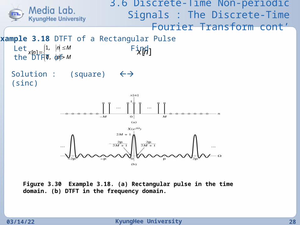
Example 3.18 DTFT of a Rectangular Pulse
Mn
Mnnx
,0
,1][ ].[nxLet Find the DTFT of
Solution : (square) (sinc)
Figure 3.30 Example 3.18. (a) Rectangular pulse in the time domain. (b) DTFT in the frequency domain.
3.6 Discrete-Time Non-periodic Signals : The Discrete-Time Fourier Transform
cont’
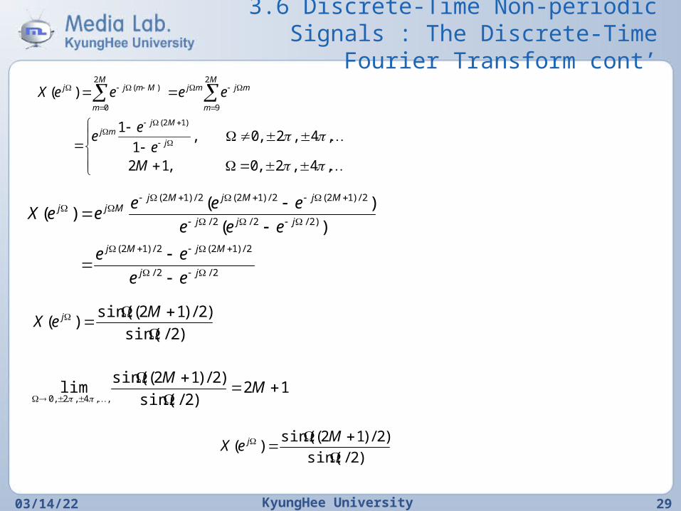
04/20/23 KyungHee University 29
,4,2,0,12
,4,2,0,1
1
)(
)12(
2
9
2
0
)(
Me
ee
eeeeX
j
Mjmj
M
m
mjmjM
m
Mmjj
2/2/
2/)12(2/)12(
)2/2/2/
2/)12(2/)12(2/)12(
)(
)()(
jj
MjMj
jjj
MjMjMjMjj
ee
ee
eee
eeeeeX
)2/sin(
)2/)12(sin()(
MeX j
12)2/sin(
)2/)12(sin(lim
,,4,2,0
M
M
)2/sin(
)2/)12(sin()(
MeX j
3.6 Discrete-Time Non-periodic Signals : The Discrete-Time Fourier Transform
cont’
04/20/23 KyungHee University 30
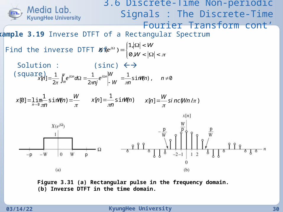
Example 3.19 Inverse DTFT of a Rectangular Spectrum
Find the inverse DTFT of
W
WeX j
,0
,1)(
Solution : (sinc) (square)
0),sin(1
2
1
2
1][
nWnnW
We
njdenx njW
W
nj
W
Wnn
xn
)sin(1
lim]0[0
)sin(1
][ Wnn
nx
)/(][
WnncsiW
nx
Figure 3.31 (a) Rectangular pulse in the frequency domain. (b) Inverse DTFT in the time domain.
3.6 Discrete-Time Non-periodic Signals : The Discrete-Time Fourier Transform
cont’
04/20/23 KyungHee University 31
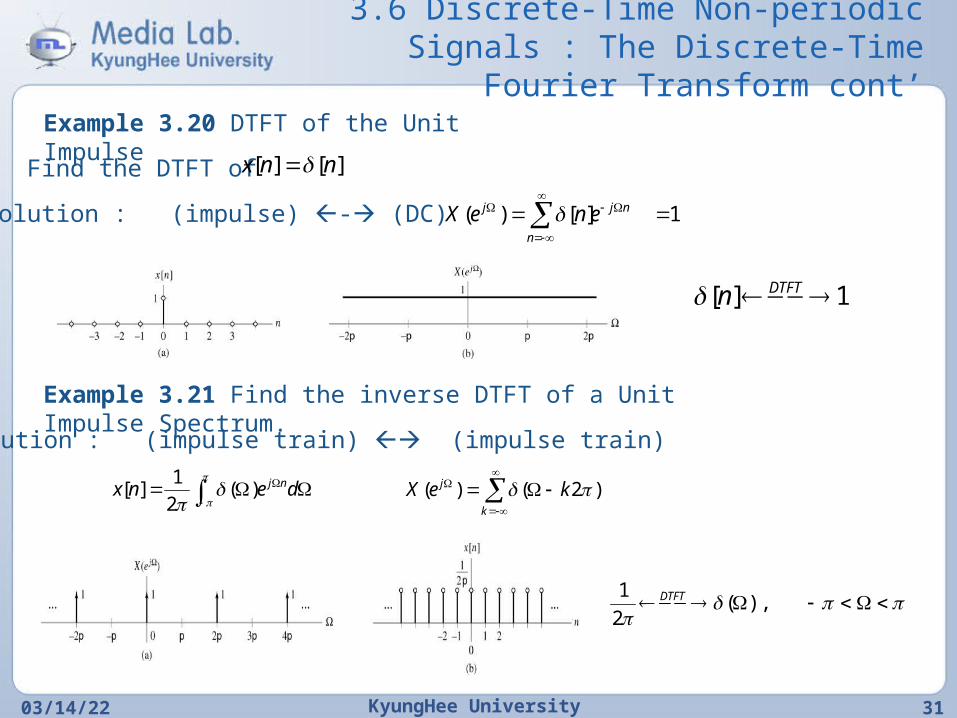
Example 3.20 DTFT of the Unit ImpulseFind the DTFT of ][][ nnx
Solution : (impulse) - (DC) 1][)(
nj
n
j eneX
1][ DTFTn
Example 3.21 Find the inverse DTFT of a Unit Impulse Spectrum.
Solution : (impulse train) (impulse train)
denx nj)(
2
1][
k
j keX )2()(
),(2
1 DTFT
3.6 Discrete-Time Non-periodic Signals : The Discrete-Time Fourier Transform
cont’
04/20/23 KyungHee University 32
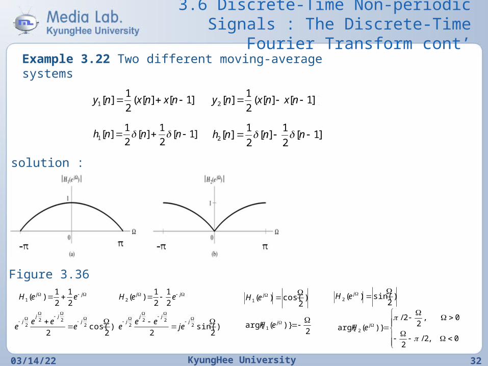
Example 3.22 Two different moving-average systems
])1[][(2
1][1 nxnxny ])1[][(
2
1][2 nxnxny
]1[2
1][
2
1][1 nnnh ]1[
2
1][
2
1][2 nnnh
solution :
Figure 3.36 jj eeH
2
1
2
1)(1
jj eeH2
1
2
1)(2
)2
cos(2
222
2
jjj
je
eee )
2sin(
22
222
jjj
jje
eee
)2
cos()(1
jeH )
2sin()(2
jeH
2)}(arg{ 1
jeH
0,2/2
0,2
2/)}(arg{ 2
jeH
3.6 Discrete-Time Non-periodic Signals : The Discrete-Time Fourier Transform
cont’
04/20/23 KyungHee University 33
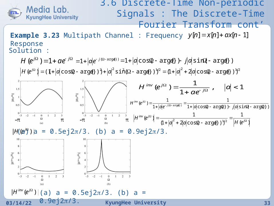
Example 3.23 Multipath Channel : Frequency Response
]1[][][ naxnxny
Solution : jj aeeH 1)( })arg{(1 ajea })arg{sin(})arg{cos(1 aajaa
2/122/1222 }))arg{cos(21(}))arg{(sin}))arg{cos(1(()( aaaaaaaeH j
1,1
1)(
aae
eHj
jinv
})arg{sin(})arg{cos(1
1
1
1)(
})arg{(
ajaeaeH
ajjinv
)(
1
}))arg{cos(21(
1)(
2/12
j
jinv
eHaaaeH
|)(| jeH (a) a = 0.5ej2/3. (b) a = 0.9ej2/3.
|)(| jinv eH (a) a = 0.5ej2/3. (b) a = 0.9ej2/3.
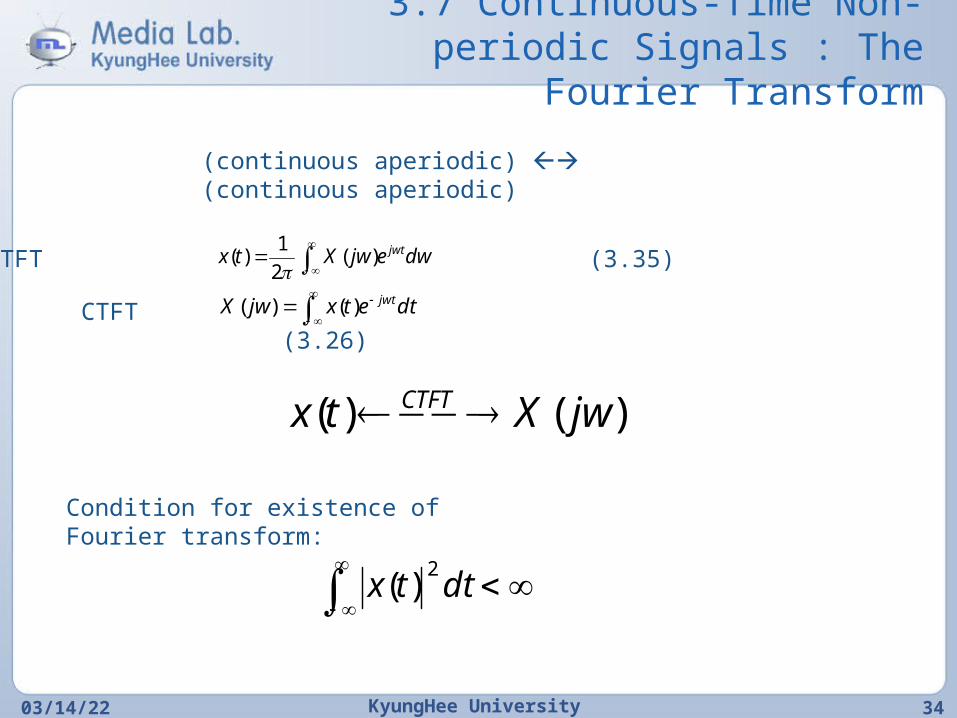
3.7 Continuous-Time Non-periodic Signals : The Fourier
Transform
04/20/23 KyungHee University 34
(continuous aperiodic) (continuous aperiodic)
Inverse CTFT (3.35)
dwejwXtx jwt)(
2
1)(
CTFT (3.26)
dtetxjwX jwt)()(
)()( jwXtx CTFT
Condition for existence of Fourier transform:
dttx
2)(
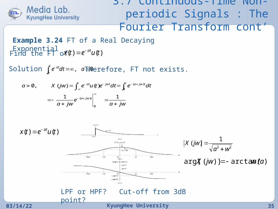
3.7 Continuous-Time Non-periodic Signals : The Fourier
Transform cont’
04/20/23 KyungHee University 35
Example 3.24 FT of a Real Decaying ExponentialFind the FT of )()( tuetx at
Solution : 0,0
adte at Therefore, FT not exists.
jwae
jwa
dtedtetuejwXa
tjwa
tjwajwtat
11
)()(,0
0
)(
0
)(
22
1)(
wajwX
)/arctan()}(arg{ awjwX
LPF or HPF? Cut-off from 3dB point?
)()( tuetx at
3.7 Continuous-Time Non-periodic Signals : The Fourier
Transform cont’
04/20/23 KyungHee University 36
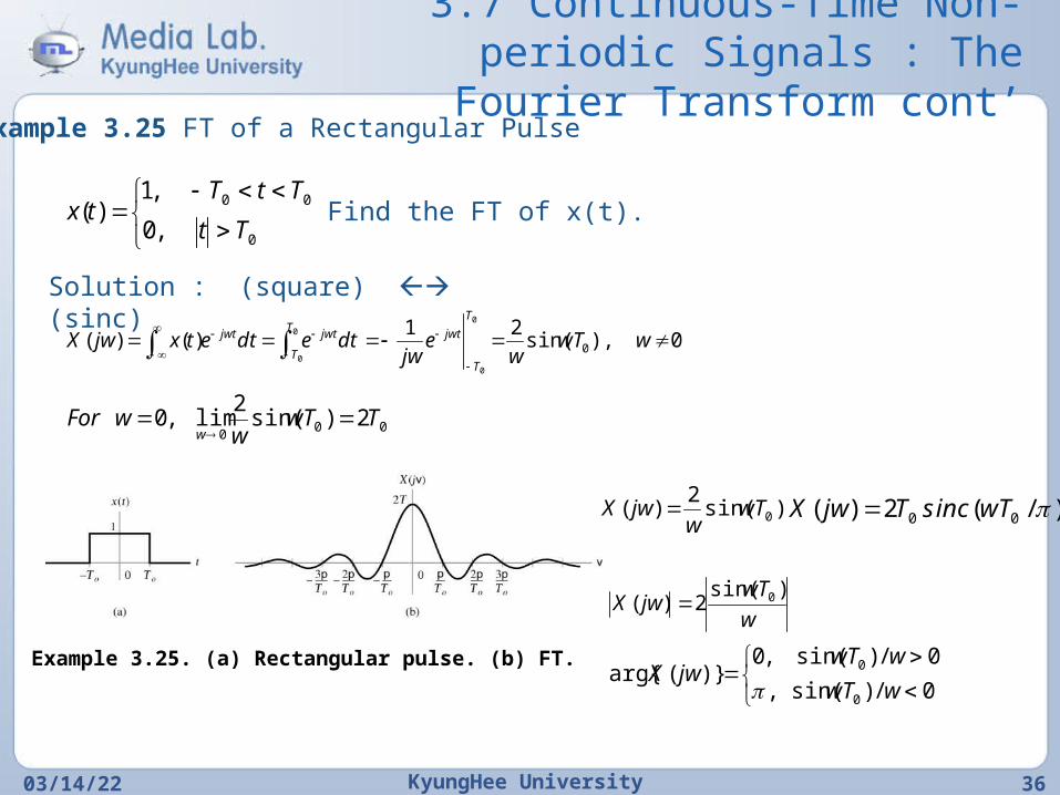
Example 3.25 FT of a Rectangular Pulse
0
00
,0
,1)(
Tt
TtTtx Find the FT of x(t).
Solution : (square) (sinc)
0),sin(21
)()( 0
0
0
0
0
wwTw
ejw
dtedtetxjwXT
T
jwtT
T
jwtjwt
000
2)sin(2
lim,0 TwTw
wForw
Example 3.25. (a) Rectangular pulse. (b) FT.
)sin(2
)( 0wTw
jwX )/(2)( 00 wTincsTjwX
w
wTjwX
)sin(2)( 0
0/)sin(,
0/)sin(,0)}(arg{
0
0
wwT
wwTjwX
3.7 Continuous-Time Non-periodic Signals : The Fourier
Transform cont’
04/20/23 KyungHee University 37
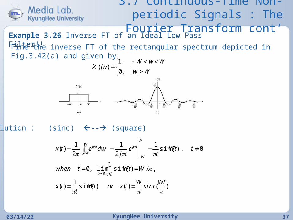
Example 3.26 Inverse FT of an Ideal Low Pass Filter!!Fine the inverse FT of the rectangular spectrum depicted in Fig.3.42(a) and given by
Ww
WwWjwX
,0
,1)(
Solution : (sinc) -- (square)
)()()sin(1
)(
,/)sin(1
lim,0
0),sin(1
2
1
2
1)(
0
Wtncsi
WtxorWt
ttx
WWtt
twhen
tWtt
etj
dwetx
t
W
W
jwtW
W
jwt
3.7 Continuous-Time Non-periodic Signals : The Fourier
Transform cont’
04/20/23 KyungHee University 38
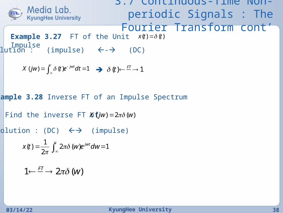
Example 3.27 FT of the Unit Impulse
)()( ttx
Solution : (impulse) - (DC)
1)()( dtetjwX jwt 1)( FTt
Example 3.28 Inverse FT of an Impulse Spectrum
Find the inverse FT of )(2)( wjwX
Solution : (DC) (impulse)
1)(22
1)(
dwewtx jwt
)(21 wFT
3.7 Continuous-Time Non-periodic Signals : The Fourier
Transform cont’
04/20/23 KyungHee University 39
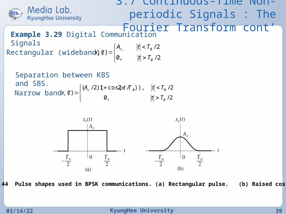
Example 3.29 Digital Communication SignalsRectangular (wideband)
2/,0
2/)(
0
0,
Tt
TtAtx
r
r
Separation between KBS and SBS. Narrow band
2/,0
2/)),/2cos(1)(2/()(
0
00
Tt
TtTtAtx
c
c
Figure 3.44 Pulse shapes used in BPSK communications. (a) Rectangular pulse. (b) Raised cosine pulse.
3.7 Continuous-Time Non-periodic Signals : The Fourier
Transform cont’
04/20/23 KyungHee University 40
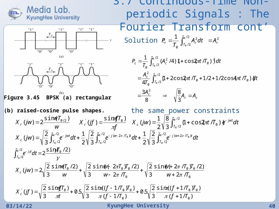
Figure 3.45 BPSK (a) rectangular pulse shapes
(b) raised-cosine pulse shapes.
Solution : 22/
2/
2
0
0
0
1r
T
T rr AdtAT
P
crc
T
T
c
T
T cc
AAA
dtTtTtT
A
dtTtAT
P
3
8
8
3
)]/4cos(2/12/1/2cos(21[4
))/2cos(1)(4/(1
2
2/
2/ 000
2
2/
2/
20
2
0
0
0
0
0
the same power constraints
w
wTjwX r
)sin(2)( 2/0
f
fTjfX r
)sin()( 0'
2/
2/ 0
0
0
))/2cos(1(3
8
2
1)(
T
T
jwtc dteTtjwX
2/
2/
)/2(2/
2/
)/2(2/
2/
0
0
00
0
00
0 3
2
2
1
3
2
2
1
3
2)(
T
T
tTwjT
T
tTwjT
T
jwtc dtedtedtejwX
)2/sin(
2 02/
2/
0
0
Tdte
T
T
tj
0
00
0
000
/2
)2/)/2sin((
3
2
/2
)2/)2sin((
3
2)2/sin(
3
22)(
Tw
TTw
Tw
TTw
w
wTjwX c
)/1(
))/1(sin(
3
25.0
)/1(
))/1(sin(
3
25.0
)sin(
3
2)(
0
00
0
000'
Tf
TTf
Tf
TTf
t
fTjfX c
3.7 Continuous-Time Non-periodic Signals : The Fourier
Transform cont’
04/20/23 KyungHee University 41
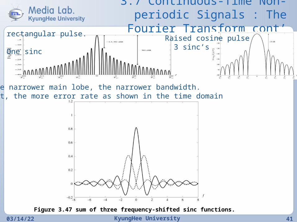
rectangular pulse.
One sinc
Raised cosine pulse 3 sinc’s
The narrower main lobe, the narrower bandwidth. But, the more error rate as shown in the time domain
Figure 3.47 sum of three frequency-shifted sinc functions.
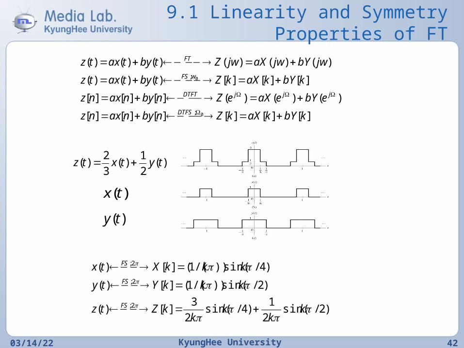
9.1 Linearity and Symmetry Properties of FT
04/20/23 KyungHee University 42
][][][][][][
)()()(][][][
][][][)()()(
)()()()()()(
0
0
;
;
kbYkaXkZnbynaxnz
ebYeaXeZnbynaxnz
kbYkaXkZtbytaxtz
jwbYjwaXjwZtbytaxtz
DTFS
jjjDTFT
wFS
FT
)(2
1)(
3
2)( tytxtz
)(tx
)(ty
)2/sin(2
1)4/sin(
2
3][)(
)2/sin())/(1(][)(
)4/sin())/(1(][)(
2;
2;
2;
kk
kk
kZtz
kkkYty
kkkXtx
FS
FS
FS
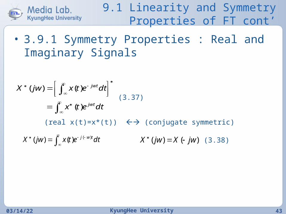
9.1 Linearity and Symmetry Properties of FT cont’
• 3.9.1 Symmetry Properties : Real and Imaginary Signals
04/20/23 KyungHee University 43
dtetx
dtetxjwX
jwt
jwt
)(
)()((3.37)
(real x(t)=x*(t)) (conjugate symmetric)
dtetxjwX twj )()()( )()( jwXjwX (3.38)
9.1 Linearity and Symmetry Properties of FT cont’
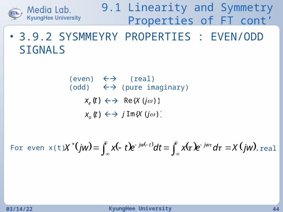
• 3.9.2 SYSMMEYRY PROPERTIES : EVEN/ODD SIGNALS
04/20/23 KyungHee University 44
(even) (real)(odd) (pure
imaginary)
)(txe )}(Re{ jX
)(txo )}(Im{ jXj
For even x(t), .* jwXdexdtetxjwX jwtjw
real
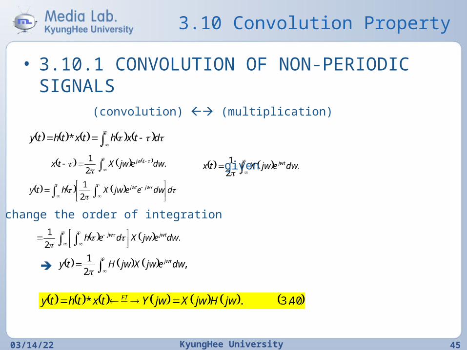
3.10 Convolution Property
• 3.10.1 CONVOLUTION OF NON-PERIODIC SIGNALS
04/20/23 KyungHee University 45
(convolution) (multiplication)
dtxhtxthty *
.2
1
dwejwXtx tjw
.
2
1
dwejwXtx jwt
But given
ddweejwXhty jwjwt
2
1
change the order of integration
.
2
1dwejwXdeh jwtjw
,
2
1dwejwXjwHty jwt
40.3.* jwHjwXjwYtxthty FT
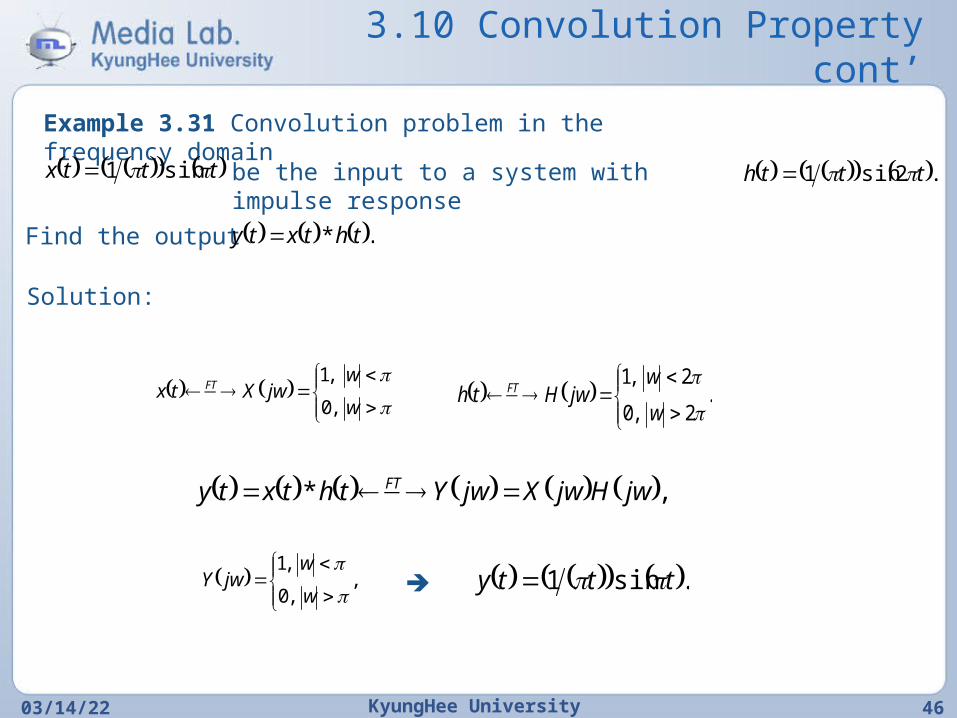
3.10 Convolution Property cont’
04/20/23 KyungHee University 46
Example 3.31 Convolution problem in the frequency domain tttx sin1 be the input to a system with impulse
response .2sin1 ttth
Find the output .* thtxty
Solution:
w
wjwXtx FT
,0
,1 .
2,0
2,1
w
wjwHth FT
,* jwHjwXjwYthtxty FT
,,0
,1
w
wjwY .sin1 ttty
3.10 Convolution Property cont’
04/20/23 KyungHee University 47
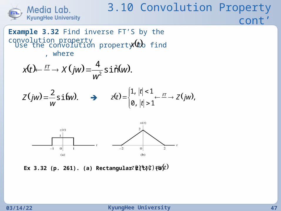
Example 3.32 Find inverse FT’S by the convolution property
Use the convolution property to find , where
tx
.sin4 2
2w
wjwXtx FT
.sin2
ww
jwZ ,1,0
1,1jwZ
t
ttz FT
Ex 3.32 (p. 261). (a) Rectangular z(t). (b) txtztz )(*)(
3.10 Convolution Property cont’
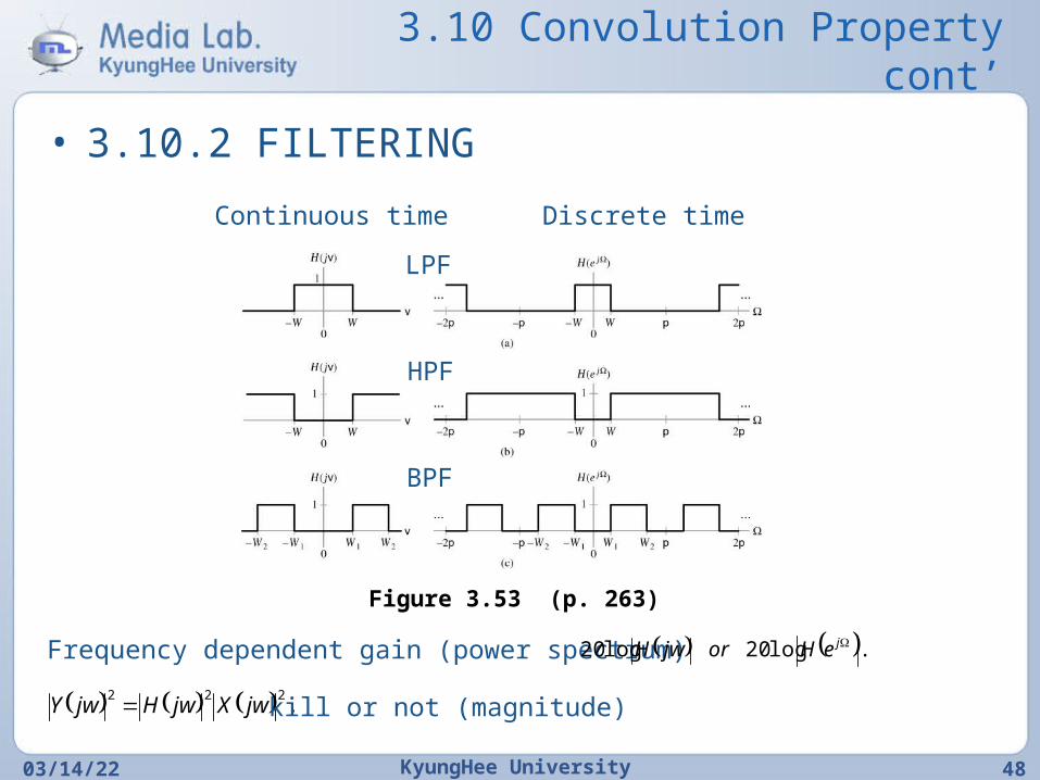
• 3.10.2 FILTERING
04/20/23 KyungHee University 48
Continuous time Discrete time
LPF
HPF
BPF
Figure 3.53 (p. 263)
Frequency dependent gain (power spectrum) .log20log20 jeHorjwH
,222
jwXjwHjwY kill or not (magnitude)
3.10 Convolution Property cont’
04/20/23 KyungHee University 49
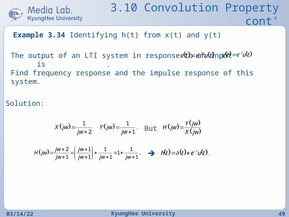
Example 3.34 Identifying h(t) from x(t) and y(t)
The output of an LTI system in response to an input is .Find frequency response and the impulse response of this system.
tuetx t2 tuety t
Solution:
2
1
jw
jwX .1
1
jw
jwY But jwX
jwYjwH
.1
11
1
1
1
1
1
2
jwjwjw
jw
jw
jwjwH .tuetth t
3.10 Convolution Property cont’
04/20/23 KyungHee University 50
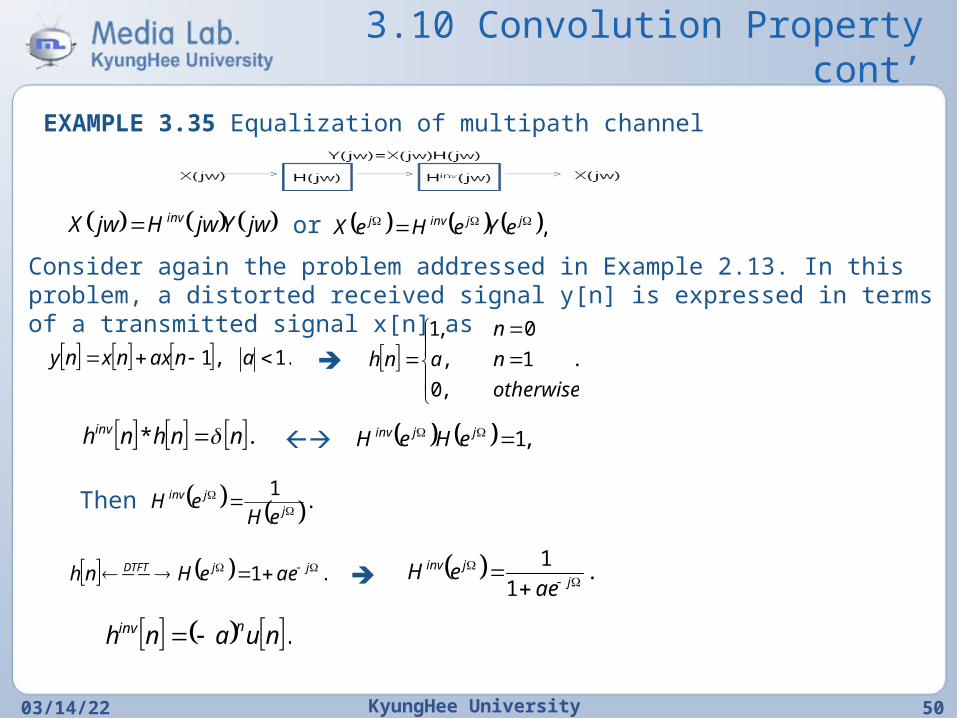
EXAMPLE 3.35 Equalization of multipath channel
jwYjwHjwX inv , jjinvj eYeHeXor
Consider again the problem addressed in Example 2.13. In this problem, a distorted received signal y[n] is expressed in terms of a transmitted signal x[n] as
.1,1 anaxnxny .
,0
1,
0,1
otherwise
na
n
nh
.* nnhnh inv ,1 jjinv eHeH
Then .1
jjinv
eHeH
.1 jjDTFT aeeHnh .1
1
j
jinv
aeeH
.nuanh ninv
3.10 Convolution Property cont’
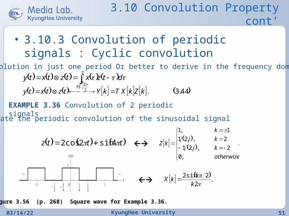
• 3.10.3 Convolution of periodic signals : Cyclic convolution
04/20/23 KyungHee University 51
Convolution in just one period Or better to derive in the frequency domain
dtzxtztxtyT
0 44.3.
2;
kZkXTkYtztxty TFS
Figure 3.56 (p. 268) Square wave for Example 3.36.
.
2
2sin2
k
kkX
EXAMPLE 3.36 Convolution of 2 periodic signals
Evaluate the periodic convolution of the sinusoidal signal
tttz 4sin2cos2 .
,0
2,21
2,21
1,1
otherwize
kj
kj
k
kZ
3.10 Convolution Property cont’
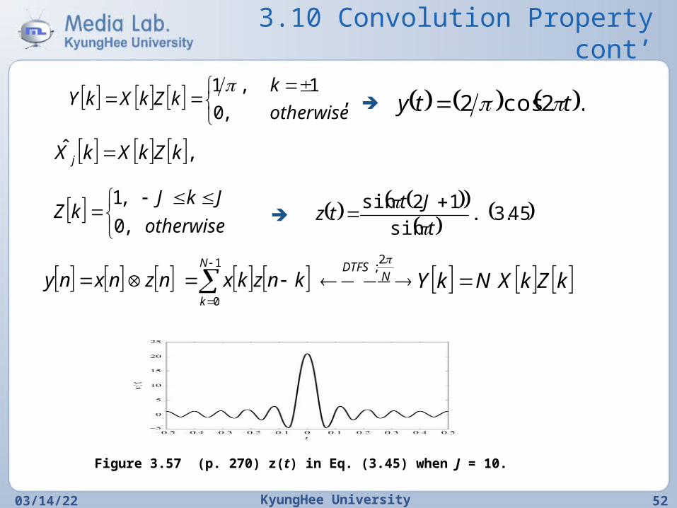
04/20/23 KyungHee University 52
Figure 3.57 (p. 270) z(t) in Eq. (3.45) when J = 10.
1
0
N
k
knzkxnznxny kZkXNkYNDTFS
2
;
otherwise
JkJkZ
,0
,1
45.3.sin
12sin
t
Jttz
,ˆ kZkXkX j
,,0
1,1
otherwise
kkZkXkY
.2cos2 tty
3.11 Differentiation and Integration Properties
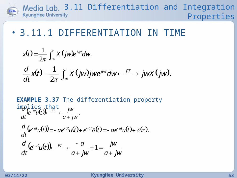
• 3.11.1 DIFFERENTIATION IN TIME
04/20/23 KyungHee University 53
.
2
1dwejwXtx jwt
dwjwejwXtx
dt
d jwt
2
1 .jwjwXFT
EXAMPLE 3.37 The differentiation property implies that
.jwa
jwtue
dt
d FTat
. tuaetetuaetuedt
d atatatat
jwa
jw
jwa
atue
dt
d FTat
1
3.11 Differentiation and Integration Properties cont’
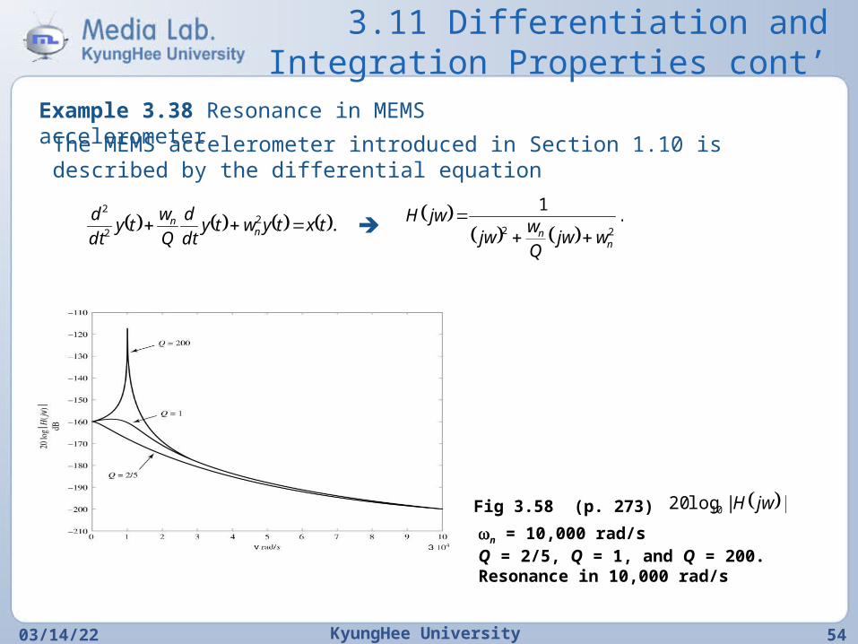
04/20/23 KyungHee University 54
Example 3.38 Resonance in MEMS accelerometerThe MEMS accelerometer introduced in Section 1.10 is described by the differential equation
.22
2
txtywtydt
d
Q
wty
dt
dn
n
.1
22n
n wjwQ
wjw
jwH
Fig 3.58 (p. 273) ||log20 10 jwH
n = 10,000 rad/sQ = 2/5, Q = 1, and Q = 200.Resonance in 10,000 rad/s
3.11 Differentiation and Integration Properties cont’
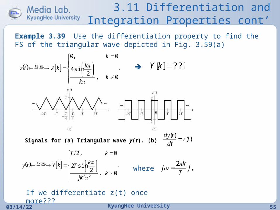
04/20/23 KyungHee University 55
Example 3.39 Use the differentiation property to find the FS of the triangular wave depicted in Fig. 3.59(a)
.
0,2
sin4
0,0
0;
k
k
k
k
kZtz wFS
???][ kY
Signals for (a) Triangular wave y(t). (b) )()(
tzdt
tdy
.
0,2sin2
0,2
22
; 0
k
jk
kT
kT
kYty wFS
,
2j
T
kj
where
If we differentiate z(t) once more???
3.11 Differentiation and Integration Properties cont’
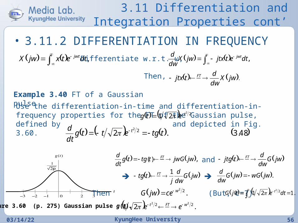
• 3.11.2 DIFFERENTIATION IN FREQUENCY
04/20/23 KyungHee University 56
,
dtetxjwX jwt Differentiate w.r.t. ω, ,
dtetjtxjwXdw
d jwt
Then, .jwXdw
dtjtx FT
Example 3.40 FT of a Gaussian pulse
Use the differentiation-in-time and differentiation-in-frequency properties for the FT of the Gaussian pulse, defined by and depicted in Fig. 3.60.
22
21 tetg
48.3.2 22
ttgettgdt
d t
Figure 3.60 (p. 275) Gaussian pulse g(t).
,)( jwjwGttgtgdt
d FT jwGdw
dtjtg FTand
jwGdw
d
jttg FT 1
.jwwGjwGdw
d
.22wcejwG Then (But, c=?) .1210 22
dtejG t
.21 22 22 wFTt ee
3.11 Differentiation and Integration Properties cont’
• 3.11.3 Integration
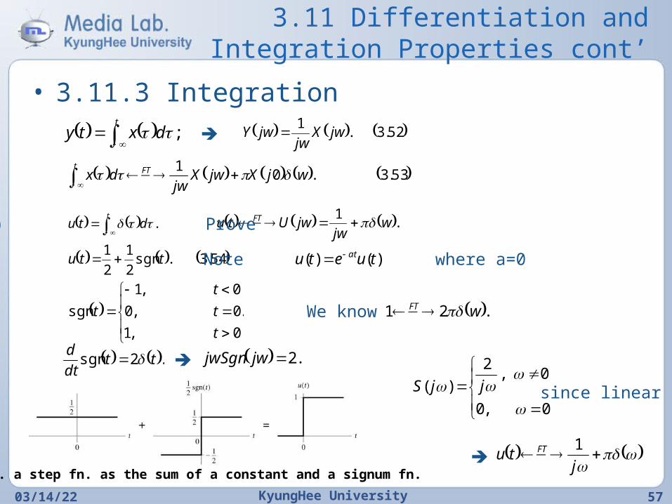
04/20/23 KyungHee University 57
;
tdxty 52.3.
1jwX
jwjwY
53.3.01
wjXjwXjw
dx FTt
.
tdtu .1
wjw
jwUtu FT Ex) Prove
54.3.sgn2
1
2
1ttu Note where a=0)()( tuetu at
.
0,1
0,0
0,1
sgn
t
t
t
t We know .21 wFT
.2sgn ttdt
d .2jwjwSgn
Fig. a step fn. as the sum of a constant and a signum fn.
0,0
0,2
)(
jjS
j
tu FT 1
since linear
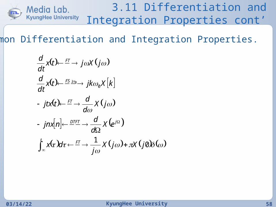
3.11 Differentiation and Integration Properties cont’
04/20/23 KyungHee University 58
Common Differentiation and Integration Properties.
01
0; 0
jXjXj
dx
eXd
dnjnx
jXd
dtjtx
kXjktxdt
d
jXjtxdt
d
FTt
jDTFT
FT
FS
FT
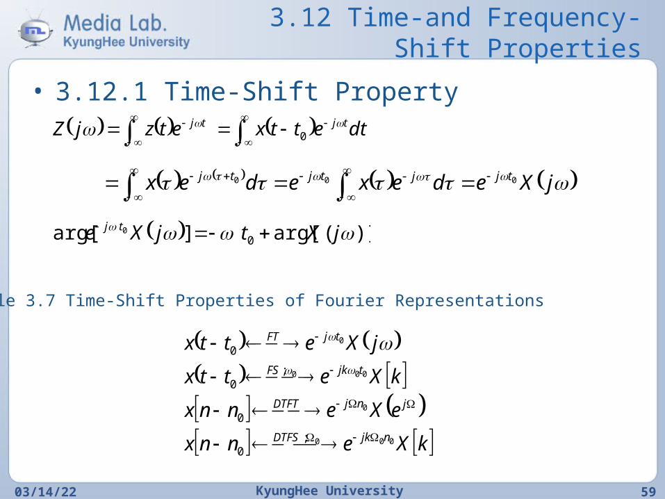
3.12 Time-and Frequency-Shift Properties
• 3.12.1 Time-Shift Property
04/20/23 KyungHee University 59
dtettxetzjZ tjtj 0
jXedexedex tjjtjtj 000
)](arg[]arg[ 0
0 jXtjXe tj
Table 3.7 Time-Shift Properties of Fourier Representations
kXennx
eXennx
kXettx
jXettx
njkDTFS
jnjDTFT
tjkFS
tjFT
000
0
000
0
;0
0
;0
0
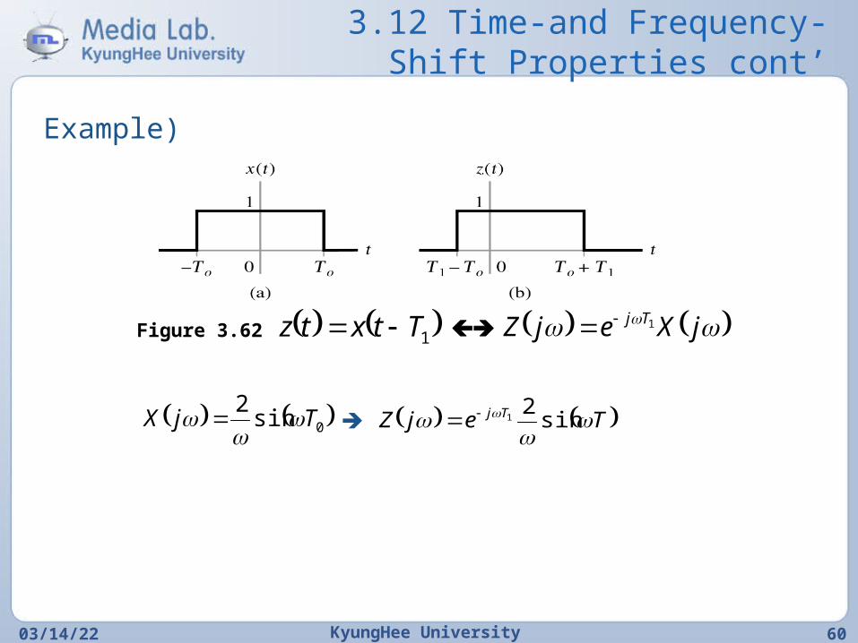
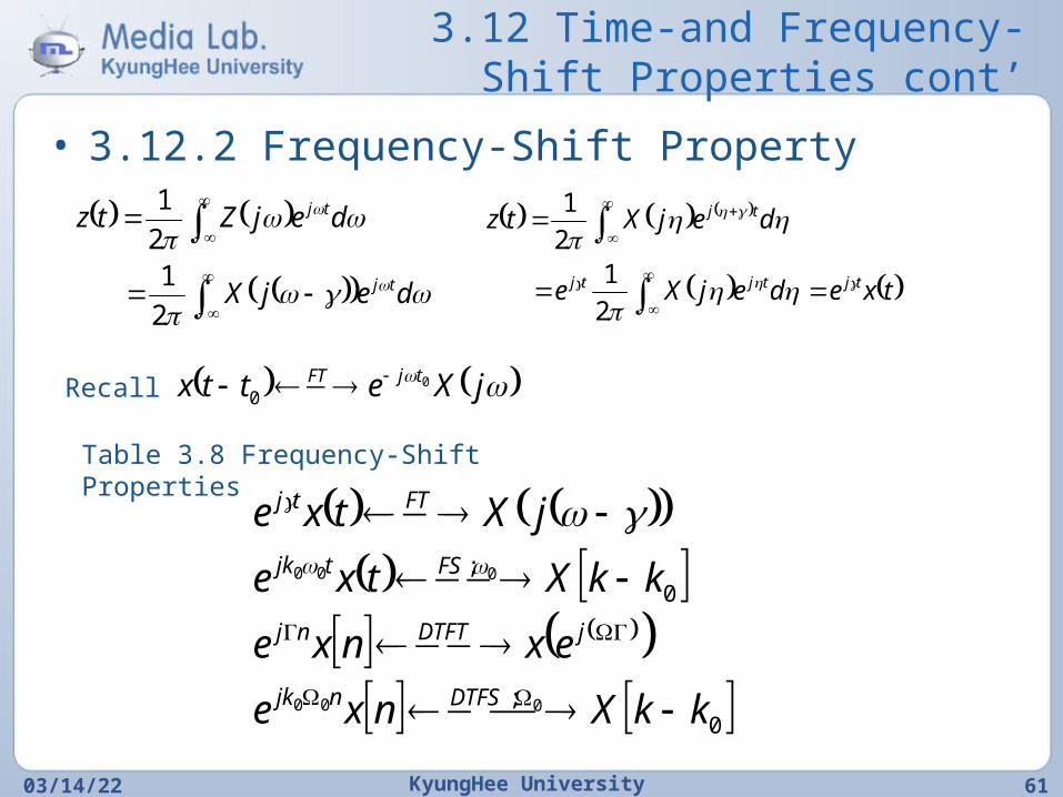
3.12 Time-and Frequency-Shift Properties cont’
04/20/23 KyungHee University 60
Example)
Figure 3.62 1Ttxtz jXejZ Tj 1
0sin2
TjX
TejZ Tj
sin2
1
3.12 Time-and Frequency-Shift Properties cont’
• 3.12.2 Frequency-Shift Property
04/20/23 KyungHee University 61
dejX
dejZtz
tj
tj
2
12
1
txedejXe
dejXtz
tjtjtj
tj
2
12
1
jXettx tjFT 00
Recall
Table 3.8 Frequency-Shift Properties
0
;
0;
000
000
kkXnxe
exnxe
kkXtxe
jXtxe
DTFSnjk
jDTFTnj
FStjk
FTtj
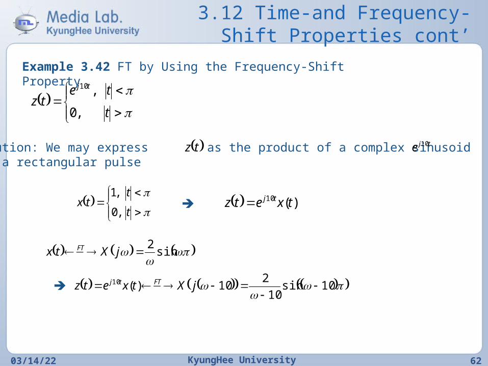
3.12 Time-and Frequency-Shift Properties cont’
04/20/23 KyungHee University 62
Example 3.42 FT by Using the Frequency-Shift Property
t
tetz
tj
,0
,10
Solution: We may express as the product of a complex sinusoid and a rectangular pulse
tz tje 10
t
ttx
,0
,1 )(10 txetz tj
sin2 jXtx FT
10sin10
210)(10
jXtxetz FTtj
3.12 Time-and Frequency-Shift Properties cont’
04/20/23 KyungHee University 63
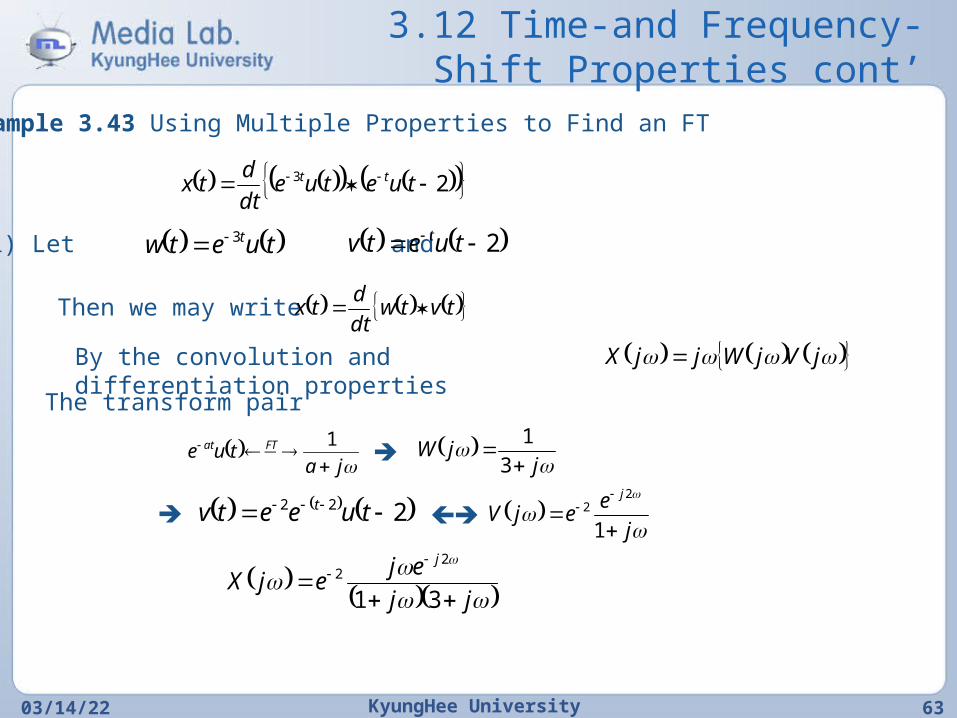
Example 3.43 Using Multiple Properties to Find an FT
23 tuetuedt
dtx tt
Sol) Let and tuetw t3 2 tuetv t
Then we may write tvtwdt
dtx
By the convolution and differentiation properties
jVjWjjX
The transform pair
ja
tue FTat
1
jjW
3
1
222 tueetv t
j
eejV
j
1
22
jj
ejejX
j
31
22
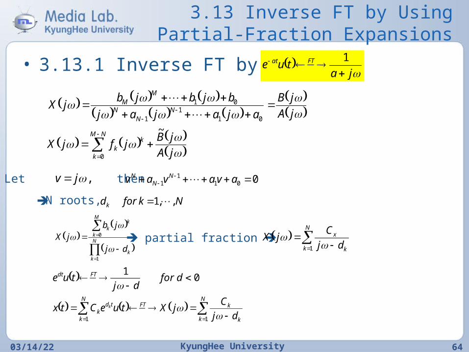
3.13 Inverse FT by Using Partial-Fraction Expansions
• 3.13.1 Inverse FT by using
04/20/23 KyungHee University 64
ja
tue FTat
1
jA
jB
ajajaj
bjbjbjX N
NN
MM
01
11
01
NM
k
kk jA
jBjfjX
0
~
Let then ,jv 0011
1 avavav N
NN
Nkfordk ,,1N roots,
N
kk
M
k
kk
dj
jbjX
1
0
partial fraction
N
k k
x
dj
CjX
1
01
dfordj
tue FTdt
N
k
N
k k
kFTtdk dj
CjXtueCtx k
1 1
3.13 Inverse FT by Using Partial-Fraction Expansions cont’
• 3.13.2 Inverse Discrete-Time Fourier Transform
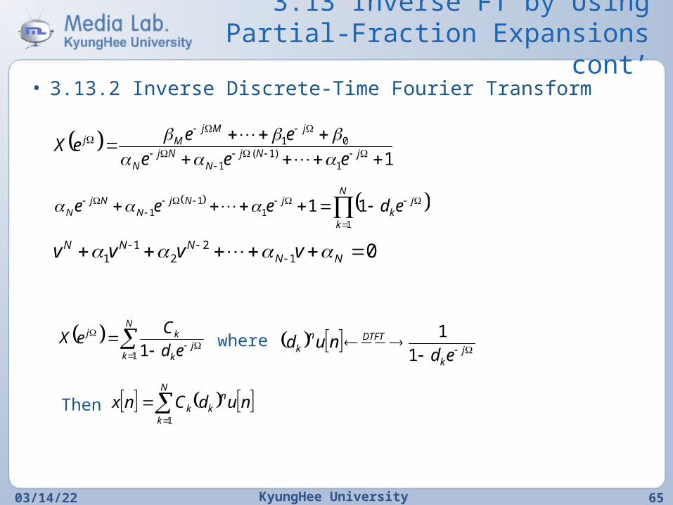
04/20/23 KyungHee University 65
11
)1(1
01
jNjN
NjN
jMjMj
eee
eeeX
N
k
jk
jNjN
NjN edeee
11
11 11
012
21
1
NNNNN vvvv
N
kj
k
kj
ed
CeX
1 1
jk
DTFTnk ed
nud1
1where
Then
N
k
nkk nudCnx
1
3.13 Inverse FT by Using Partial-Fraction Expansions cont’
04/20/23 KyungHee University 66
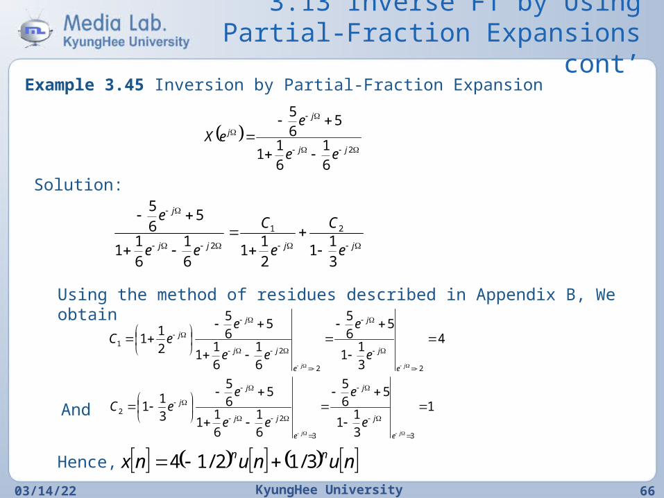
Example 3.45 Inversion by Partial-Fraction Expansion
2
6
1
6
11
56
5
jj
j
j
ee
eeX
Solution:
jjjj
j
e
C
e
C
ee
e
3
11
2
11
6
1
6
11
56
5
21
2
Using the method of residues described in Appendix B, We obtain
4
3
11
56
5
6
1
6
11
56
5
2
11
22
21
jj e
j
j
e
jj
j
j
e
e
ee
eeC
1
3
11
56
5
6
1
6
11
56
5
3
11
33
22
jj e
j
j
e
jj
j
j
e
e
ee
eeCAnd
Hence, nununx nn 3/12/14
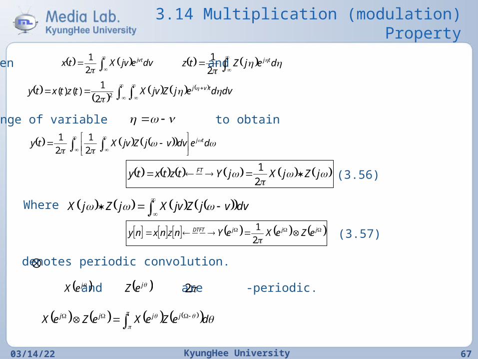
3.14 Multiplication (modulation) Property
04/20/23 KyungHee University 67
Given and
dvejvXtx jvt
2
1
dejZtz tj
2
1
dvdejZjvXtztxty tvj
22
1)()(
Change of variable to obtain
dedvvjZjvXty tj
2
1
2
1
jZjXjYtztxty FT 2
1
dvvjZjvXjZjX Where
jjjDTFT eZeXeYnznxny2
1
(3.56)
(3.57)
denotes periodic convolution.
Here, and are -periodic. jeX jeZ 2
deZeXeZeX jjjj
3.14 Multiplication (modulation) Property cont’
04/20/23 KyungHee University 68
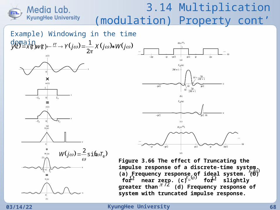
Example) Windowing in the time domain
jWjXjYtwtxty FT
2
1)()(
0sin2
TjW
Figure 3.66 The effect of Truncating the impulse response of a discrete-time system. (a) Frequency response of ideal system. (b) for near zero. (c) for slightly greater than (d) Frequency response of system with truncated impulse response.
F
F 2/
3.14 Multiplication (modulation) Property cont’
04/20/23 KyungHee University 69
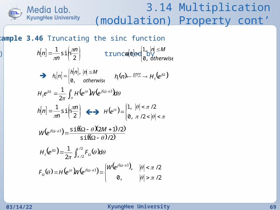
Example 3.46 Truncating the sinc function
Sol) truncated by
2sin
1 n
nnh
otherwise
Mnnw
,0
,1
otherwise
Mnnhnht
,0
, jt
DTFTt eHnh
deWeHeH jjjt 2
1
2sin
1 n
nnh
2/,0
2/,1jeH
2/sin
2/12sin
MeW j
2/
2/2
1
dFeH j
t
2/,0
2/,
j
jjeW
eWeHF
3.14 Multiplication (modulation) Property cont’
04/20/23 KyungHee University 70
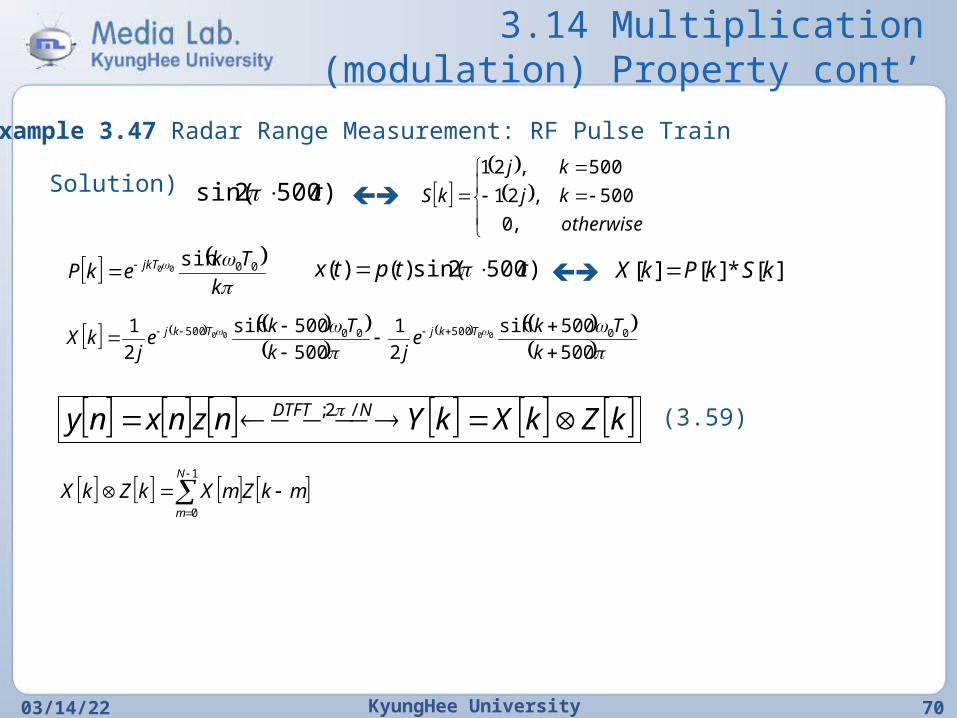
Example 3.47 Radar Range Measurement: RF Pulse Train
Solution) )5002sin( t
otherwise
kj
kj
kS
,0
500,21
500,21
k
TkekP jkT 00sin
00 )5002sin()()( ttptx ][*][][ kSkPkX
500
500sin
2
1
500
500sin
2
1 0050000500 0000
k
Tkejk
Tkej
kX TkjTkj
kZkXkYnznxny NDTFT /2; (3.59)
1
0
N
m
mkZmXkZkX
3.14 Multiplication (modulation) Property cont’
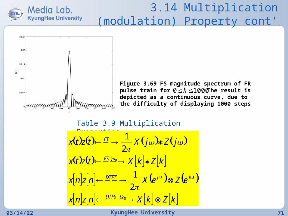
04/20/23 KyungHee University 71
Figure 3.69 FS magnitude spectrum of FR pulse train for The result is depicted as a continuous curve, due to the difficulty of displaying 1000 steps
10000 k
Table 3.9 Multiplication Properties
kZkXnznx
eZeXnznx
kZkXtztx
jZjXtztx
DTFS
jjDTFT
FS
FT
0
0
;
;
2
1
2
1
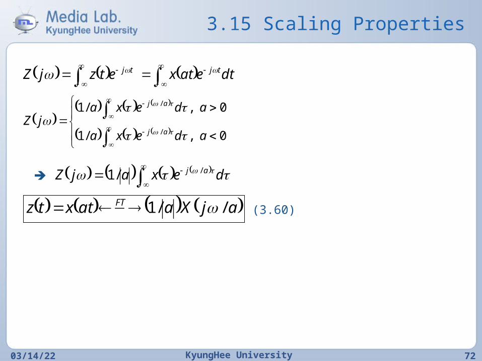
3.15 Scaling Properties
04/20/23 KyungHee University 72
dteatxetzjZ tjtj
0,/1
0,/1
/
/
adexa
adexajZ
aj
aj
dexajZ aj //1
ajXaatxtz FT //1 (3.60)
3.15 Scaling Properties cont’
04/20/23 KyungHee University 73
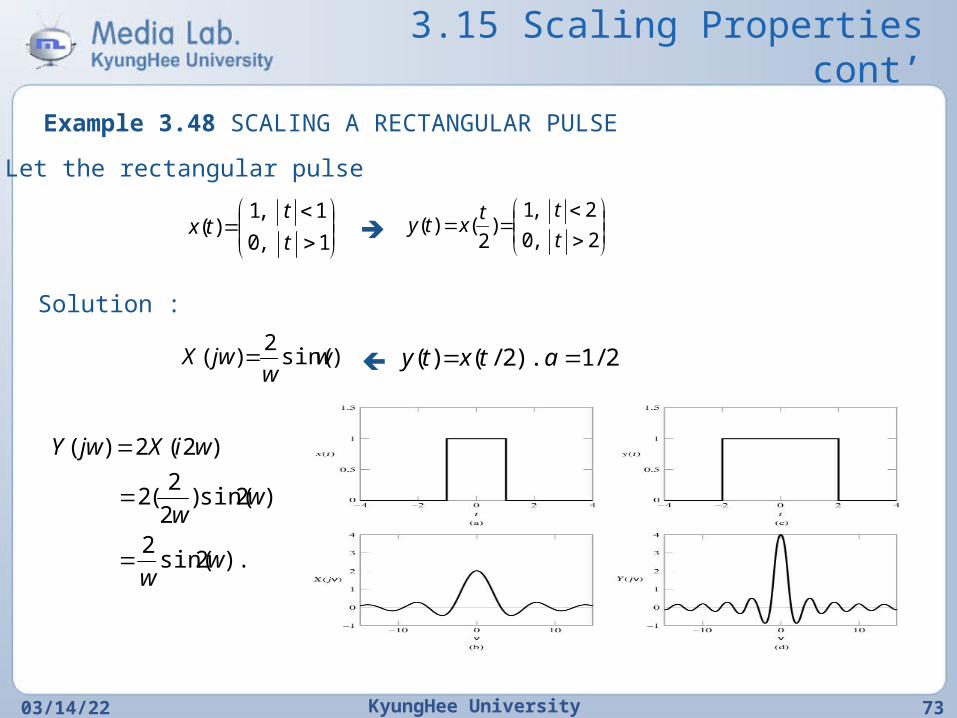
Example 3.48 SCALING A RECTANGULAR PULSE
Let the rectangular pulse
1,0
1,1)(
t
ttx
2,0
2,1)
2()(
t
ttxty
Solution :
).sin(2
)( ww
jwX 2/1).2/()( atxty
).2sin(2
)2sin()2
2(2
)2(2)(
ww
ww
wiXjwY
3.15 Scaling Properties cont’
04/20/23 KyungHee University 74
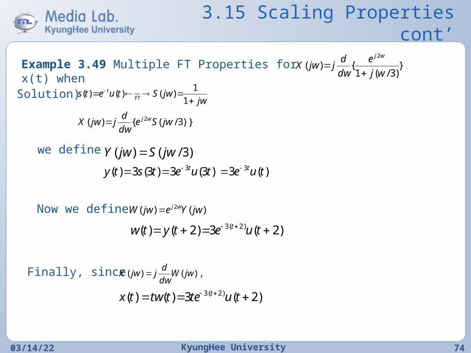
Example 3.49 Multiple FT Properties for x(t) when
}.)3/(1
{)(2
wj
e
dw
djjwX
wj
Solution)jw
jwStuetsFT
t
1
1)()()(
)}.3/({)( 2 jwSedw
djjwX wj
we define )3/()( jwSjwY ).(3)3(3)3(3)( 33 tuetuetsty tt
Now we define )()( 2 jwYejwW wj
).2(3)2()( )2(3 tuetytw t
Finally, since ),.()( jwWdw
djjwX
).2(3)()( )2(3 tutettwtx t
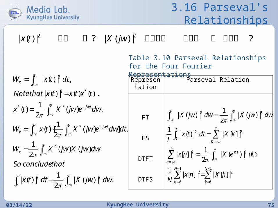
3.16 Parseval’s Relationships
04/20/23 KyungHee University 75
? |)(|?|)(| 22 에너지쓴주자가바이올린꽝언제 jwXtx
.|)(|2
1|)(|
)()(2
1
.])(2
1)[(
.)(2
1)(
).()(|)(|
,|)(|
22
*
*
**
*2
2
dwjwXdttx
thatconcludeSo
dwjwXjwXW
dtdwejwXtxW
dwejwXtx
txtxtxthatNote
dttxW
x
jwtx
jwt
x
Representation
Parseval Relation
FT
FS
DTFT
DTFS
1
0
21
0
2
22
22
22
|][||][|1
|)(|2
1|][|
|][||)(|1
|)(|2
1|)(|
N
k
N
K
j
n
K
T
O
kXnxN
deXnx
kXdttxT
dwjwXdwjwX
Table 3.10 Parseval Relationships for the Four Fourier Representations
3.16 Parseval’s Relationships cont’
04/20/23 KyungHee University 76
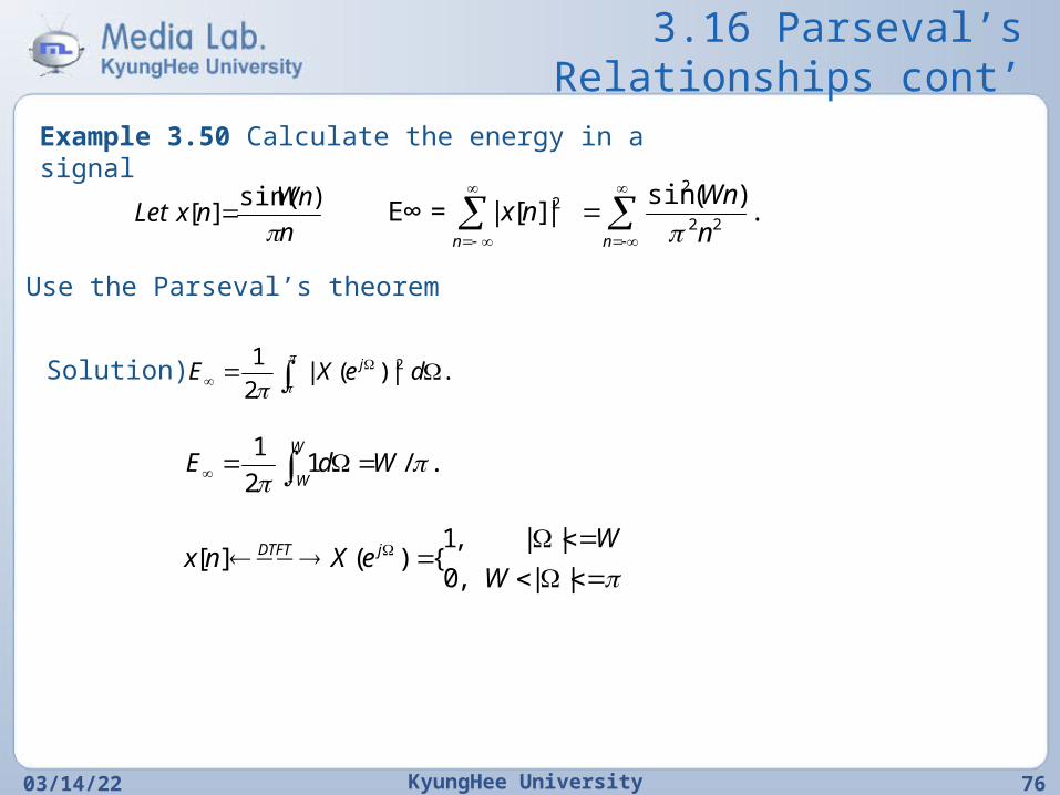
Example 3.50 Calculate the energy in a signal
n
WnnxLet
)sin(
][
nn n
Wnnx .
)(sin|][|=∞E
22
22
Use the Parseval’s theorem
Solution)
.|)(|
2
1 2 deXE j
./12
1
WdEW
W
||,0
||,1{)(][
W
WeXnx jDTFT
3.17 Time –Bandwidth Product
04/20/23 KyungHee University 77
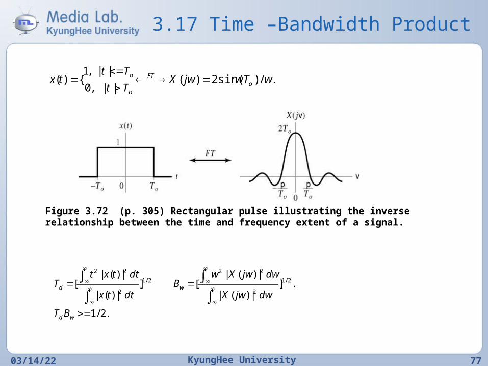
./)sin(2)(||,0
||,1{)( wwTjwX
Tt
Tttx o
FT
o
o
Figure 3.72 (p. 305) Rectangular pulse illustrating the inverse relationship between the time and frequency extent of a signal.
.2/1
.]|)(|
|)(|[]
|)(|
|)(|[ 2/1
2
22
2/1
2
22
wd
wd
BT
dwjwX
dwjwXwB
dttx
dttxtT
3.17 Time –Bandwidth Product cont’
04/20/23 KyungHee University 78
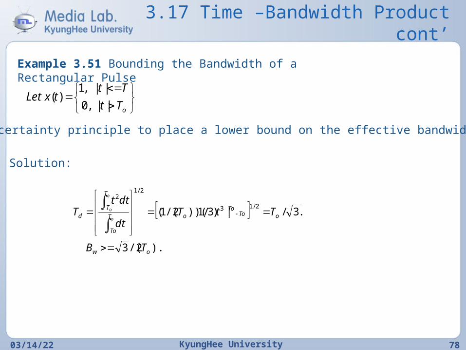
Example 3.51 Bounding the Bandwidth of a Rectangular Pulse
oTt
TttxLet
||,0
||,1)(
Use the uncertainty principle to place a lower bound on the effective bandwidth of x(t).
Solution:
).2/(3
.3/|)3/1))(2/(1(2/13
2/12
ow
oToTo
oT
To
T
Td
TB
TtTdt
dttT
o
o
o
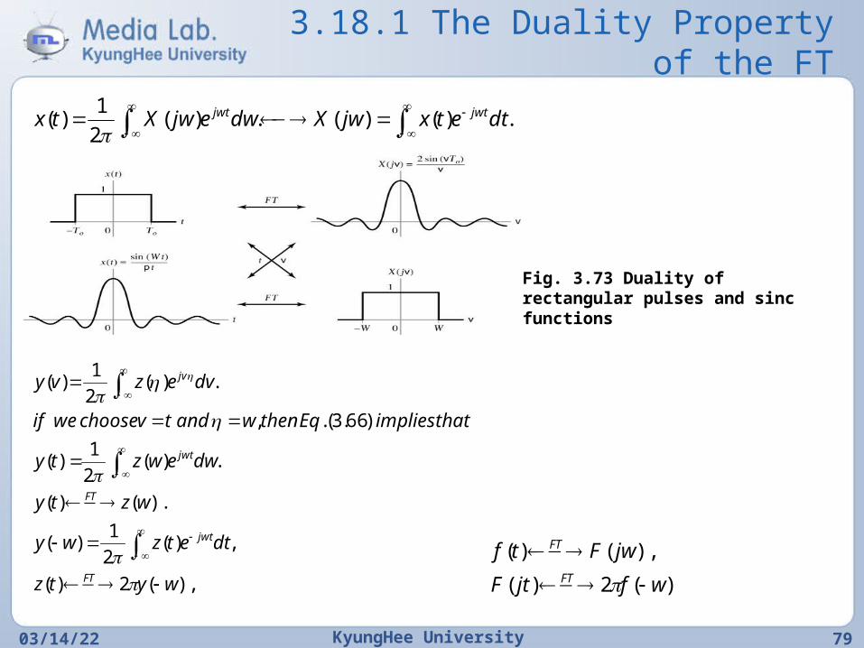
3.18.1 The Duality Property of the FT
04/20/23 KyungHee University 79
.)()(.)(2
1)( dtetxjwXdwejwXtx jwtjwt
Fig. 3.73 Duality of rectangular pulses and sinc functions
),(2)(
,)(2
1)(
).()(
.)(2
1)(
)66.3(.,
.)(2
1)(
wytz
dtetzwy
wzty
dwewzty
thatimpliesEqthenwandtvchooseweif
dvezvy
FT
jwt
FT
jwt
jv
).(2)(
),()(
wfjtF
jwFtfFT
FT
3.18.1 The Duality Property of the FT cont’
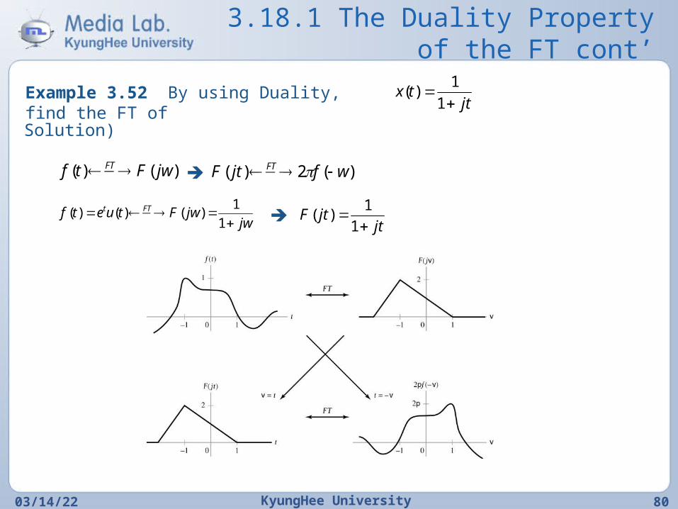
04/20/23 KyungHee University 80
Example 3.52 By using Duality, find the FT of
jttx
1
1)(
Solution)
)()( jwFtf FT ).(2)( wfjtF FT
jwjwFtuetf FTt
1
1)()()(
jtjtF
1
1)(
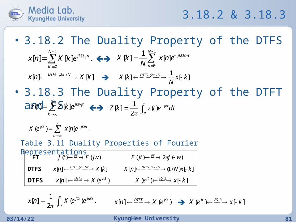
3.18.2 & 3.18.3
• 3.18.2 The Duality Property of the DTFS
• 3.18.3 The Duality Property of the DTFT and FS
04/20/23 KyungHee University 81
.][][1
0
N
K
njk oekXnx
1
0
][1
][N
n
onjkenxN
kX
][][ /2; kXnx NDTFS ][1
][ /2; kxN
kX NDTFS
k
tjkwekZtz 0][)(
dtetzkZ jkt)(
2
1][
n
njj enxeX .][)(
)(2)()()( wfjtFjwFtf FTFT FT
][)/1(][][][ /2;/2; kxNnXkXnx NDTFSNDTFS DTFS
][)()(][ 1; kxeXeXnx FSjtjDTFS DTFS
Table 3.11 Duality Properties of Fourier Representations
.)(
2
1][ jnj eeXnx )(][ jDTFT eXnx ].[)( 1; kxeX FSjt
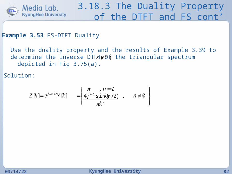
3.18.3 The Duality Property of the DTFT and FS cont’
04/20/23 KyungHee University 82
Example 3.53 FS-DTFT Duality
Use the duality property and the results of Example 3.39 to determine the inverse DTFT of the triangular spectrum depicted in Fig 3.75(a).
)( jeX
Solution:
0,)2/sin(40,
][][2
12/ n
k
kjn
kYekZ kjw
Top Related