


Languages
Pages
Legal


* Corresponding author. Manning School of Business, 1 University Avenue, University of Massachusetts Lowell,
Lowell, MA 01854, Tel: +1.978.934.2520, email: [email protected].
** C. T. Bauer College of Business, 334 Melcher Hall, University of Houston, Houston, TX, 77204, Tel:
+1.713.743. 0893, email: [email protected].
Short Selling around the 52-Week and Historical Highs
Eunju Lee* and Natalia Piqueira
**
February 2015
ABSTRACT
Although the distance of a stock price to its past price high does not provide fundamental-related
information, it plays an important role of anchoring investors' expectations in the equity market.
Using a stock's 52-week and historical highs, we examine the impact of the nearness to the price
highs on short sellers’ trading behavior in the equity market. We find that short selling is
negatively associated with the nearness of the price to the 52-week high, while it is positively
associated with the nearness to the historical high. This can be explained by biases associated
with these two anchors. That is, short sellers trade on investors' underreaction to bad news when
the stock price is far from its 52-week high and overreaction to good news when the price is near
the historical high. We also find that such short-selling activity leads to weaker momentum and
reversals in future returns, contributing to the price discovery process and to the improvement of
market quality. Overall, we conclude that short sellers are not susceptible to anchoring biases
related to the 52-week and historical highs. Rather, they are able to exploit other investors'
behavioral biases by utilizing different strategies based on relative price levels to the 52-week
and historical highs.
Short Selling around the 52-Week and Historical Highs
ABSTRACT
Although the distance of a stock price to its past price high does not provide fundamental-related
information, it plays an important role of anchoring investors' expectations in the equity market.
Using a stock's 52-week and historical highs, we examine the impact of the nearness to the price
highs on short sellers’ trading behavior in the equity market. We find that short selling is
negatively associated with the nearness of the price to the 52-week high, while it is positively
associated with the nearness to the historical high. This can be explained by biases associated
with these two anchors. That is, short sellers trade on investors' underreaction to bad news when
the stock price is far from its 52-week high and overreaction to good news when the price is near
the historical high. We also find that such short-selling activity leads to weaker momentum and
reversals in future returns, contributing to the price discovery process and to the improvement of
market quality. Overall, we conclude that short sellers are not susceptible to anchoring biases
related to the 52-week and historical highs. Rather, they are able to exploit other investors'
behavioral biases by utilizing different strategies based on relative price levels to the 52-week
and historical highs.

1
1. Introduction
A record-high stock price, such as a monthly high or a 52-week high, has become an important
factor that affects behavior of market participants and corporate managers. Prior studies
document that the price high affects not only investors' trading behavior (George and Hwang
2004; Grinblatt and Keloharju 2001; Huddart, Lang, and Yetman 2009; Li and Yu 2012) but also
managers' decision making such as stock option exercise (Heath, Huddart, and Lang 1999;
Poteshman and Serbin 2003) and mergers and acquisitions (Baker, Pan, and Wurgler 2012).
These studies suggest that their findings can be explained by psychological heuristics, such as an
adjustment and anchoring bias (Tversky and Kahneman 1974) and prospect theory (Kahneman
and Tversky 1979). Given that such behavioral biases cause mispricing such as momentum and
reversals in stock returns, trading strategies that exploit these biases can generate trading profits.
We focus on the effect of two different price highs on short sellers' behavior in this study: the 52-
week high and the historical high, which are publicly available through the financial media.1
Comparing a stock's current price with these price highs provides information about relative
price levels to past highest prices, but not about fundamental changes. In spite of that, prior
literature finds that these two price highs are used as anchors when investors evaluate
information.2 In the case of the 52-week high, investors tend to underreact to good news when
the current price is near the 52-week high and underreact to bad news when the stock price is far
from its 52-week high (George and Hwang 2004). On the other hand, the anchoring behavior
based on the historical high is found to be the opposite: investors tend to overreact to good news
when the stock price is close to its historical high and overreact to bad news when the price is far
from the historical high (Li and Yu 2012).
Taken together, the nearness of a stock price to its 52-week and historical highs indicates not
only the relative levels of current prices but also the presence of investors' anchoring bias. This
raises the question of how this price information influences trading behavior of informed traders.
Intuitively, informed traders should be able to exploit other investors' behavioral biases based on
1 While the 52-week high is the readily available information released through the media such as the Wall Street
Journal, the historical high can be obtained from historical prices data provided by the financial websites such as
Yahoo! Finance. 2 This is somewhat in line with Kahneman and Tversky (1973) and Tversky and Kahneman (1971), who argue that
investors expect trends to continue or to be reversed on a case-by-case basis.

2
the nearness to the 52-week and historical highs. However, we cannot rule out the possibility that
even informed traders are also subject to behavioral biases.
Motivated by this, we examine how short sellers react to the nearness of a stock price to the 52-
week and historical highs. An extensive literature has documented that short sellers are informed.
If short sellers are sophisticated enough to identify investors' anchoring biases associated with
the 52-week and historical highs, they will trade on underreaction to bad news when the price is
far from the 52-week high and overreaction to good news when the price is close to the historical
high. We refer to this as the behavioral exploitation hypothesis.
We also consider two additional hypotheses on short sellers' behavior on the nearness to the 52-
week and historical highs. Given the previous finding of contrarian patterns in short selling, we
can conjecture that short-selling activities simply depend on the price levels relative to the past
price highs. When the recent price is close to the 52-week or historical high, short sellers will
increase their trading in anticipation of price reversals. This hypothesis is referred to as the
contrarian short selling hypothesis. Alternatively, short sellers may be subject to anchoring
biases based on the 52-week and historical highs like other investors.3 In this case, they will
underreact based on the nearness to the 52-week high and overreact based on the nearness to the
historical high. We label this the biased short selling hypothesis.
We find that short selling is negatively associated with the nearness to the 52-week high, while it
is positively associated with the nearness to the historical high. In other words, short sellers
increase their trading when a stock price is far from its 52-week high and close to the historical
high. These findings support the behavioral exploitation hypothesis, suggesting that short sellers
are able to exploit other investors' underreaction to bad news when the price is far from the 52-
week high and overreaction to good news when the price is close to the historical high. Our
results also refute the remaining two hypotheses, showing that short sellers do not simply trade
based on recent price levels and they are not subject to anchoring biases. These findings are in
line with previous claims that sophisticated traders are less likely to be susceptible to behavioral
biases and tend to exploit the misperceptions of the uninformed (De Long, Shleifer, Summers,
and Waldmann 1990; Grinblatt and Keloharju 2001; Hong, Jordan, and Liu 2012). This pattern is
3 Even though this hypothesis seems to contradict the prevailing view that informed traders are less likely to be
subject to behavioral biases, we argue that short sellers can be susceptible to behavioral biases unless all short
sellers are informed and have perfect information about fundamental value. Some recent studies support our
argument by finding evidence of behavioral biases in informed trading (Feng and Seasholes 2005; Watson and
Funck 2012; Beschwitz and Massa 2013). We discuss this in more detail in Section 3.
3
robust when we control for past short-term momentum and other variables, such as share
turnover, price volatility, and institutional ownership.
Further, we examine if such shorting behavior based on the nearness to the 52-week and
historical highs contributes to price discovery by correcting mispricing quickly. If the above
findings are driven by informed short sellers who exploit other investors' anchoring biases,
stocks with high short-selling activity will have weaker momentum and reversals in subsequent
returns when the price is far from the 52-week high and close to the historical high.
Consistent with our expectations, we find weaker negative momentum in returns for heavily
shorted stocks when their prices are far from the 52-week highs. When stocks' prices are near the
historical highs, negative reversals even disappear for stocks with high short-selling activity.
These results suggest that aggressive shorting behavior based on the nearness to the 52-week and
historical highs contributes to correcting mispricing driven by investors' anchoring biases. This is
in line with the results in Boehmer and Wu (2013), which show that high levels of short sales
reduce post-earnings-announcement drift following negative earnings surprises.
To the best of our knowledge, this study is the first to investigate short sellers' trading behavior
based on the nearness to the 52-week and historical highs. Although several studies document
the profitability of trading strategies based on the nearness to the 52-week high (George and
Hwang 2004; Du 2008; Huddart, Lang, and Yetman 2009; Hong, Jordan, and Liu 2012) and the
historical high (Li and Yu 2012), there is no study that examines how short sellers exploit these
price extremes. Moreover, given previous findings indicating that short sellers are informed, we
provide important insights into the trading behavior of informed traders and their anchoring
biases associated with the 52-week and historical highs, which have not been examined yet.
Our findings about the relationship between short selling and the nearness to the 52-week and
historical highs also contribute to the short-selling and behavioral finance literature in two ways.
First, while existing studies mainly focus on short sellers' reaction to corporate events, such as
earnings announcements (Christophe, Ferri, and Angel 2004) or seasoned equity offerings
(Henry and Koski 2010), we examine how short sellers exploit the past price extremes, which are
publicly available information reported everyday in the financial media.
Second, we use the distances of a stock's current price to the past price highs as proxies for
under- and overreaction caused by anchoring biases. These proxies are differentiated from short-
term momentum in prior studies. While short-term momentum may indicate overreaction or

4
underreaction to news depending on the timing of information arrival, the nearness to the past
price highs and the subsequent return patterns imply both the timing of information flows and the
investors' reactions to news. This is confirmed by our findings of a positive relationship between
the nearness to the 52-week high and future returns and a negative relationship between the
nearness to the historical high and future returns. In short, the nearness to the 52-week and
historical highs facilitates the distinction between under- and overreaction, so that we can
investigate if short sellers identify investors' anchoring biases that lead to different patterns in
subsequent returns.
The remainder of this paper is organized as follows. Section 2 reviews prior literature related to
our study, and Section 3 explains our hypotheses on how short sellers react to the nearness to the
52-week and historical highs. Section 4 describes data and methodology, Section 5 explains
return patterns that are associated with the nearness to the 52-week and historical highs, and
Section 6 discusses our empirical results of short sales when the stock price is close to or far
from its 52-week and historical highs. Section 7 addresses the impact of short sales on return
momentum and reversals associated with the 52-week and historical highs, and Section 8
discusses additional tests using subsamples. Finally, Section 9 concludes the paper.
2. Related literature
2.1. Informed Short Selling
An extensive literature provides empirical evidence on informed short selling. The literature on
short sellers' information advantage can be divided into three strands. The first strand of the
literature investigates if short sellers possess private information on upcoming negative events
and take advantage of it prior to the announcements. Using an event study analysis, these studies
find high levels of short selling prior to the release of negative information that adversely affects
firms' fundamental values. Christophe, Ferri, and Angel (2004) find an increase in short selling
five days prior to negative earnings news, and Desai, Krishnamurthy, and Venkataraman (2006)
show that short sellers increase their shorting prior to earnings restatements. Similar findings are
documented with different corporate events, such as financial misconduct (Karpoff and Lou

5
2010), analyst downgrades (Christophe, Ferri, and Hsieh 2010), and credit rating downgrades
(Henry, Kisgen, and Wu 2014).
The second strand of the literature also runs event studies using corporate events, but focusing on
short-selling activities following the announcements. These studies emphasize short sellers'
superior ability to process public information. Engelberg, Reed, and Ringgenberg (2012) find
high levels of shorts following several news announcements, and Boehmer and Wu (2013) show
that short sellers exploit post-earnings-announcement drift following negative earnings surprises.
The findings of these studies suggest that short sellers are able to exploit underreaction to
negative news.
The third strand of the literature finds evidence on contrarian short selling. Diether, Lee, and
Werner (2009) show that the combination of the positive relationship between short selling and
past returns and the negative relationship between short selling and future returns provides
evidence of contrarian short selling. Based on these findings, they argue that short sellers are
able to trade on short-term overreaction. Kelley and Tetlock (2013) also find similar patterns in
retail short sales.
Overall, the above studies focus on examining shorting behavior based on return patterns and
corporate events, but none of them have investigated short-selling activities around past price
extremes, which play an important role when we analyze behavioral biases.
2.2. Reference Point Effects: Prospect Theory and Anchoring Bias
An individual's propensity to use reference points to evaluate gains and losses can be explained
by prospect theory and the anchoring bias. Prospect theory proposed by Kahneman and Tversky
(1979) pinpoints an S-shaped value function. The important feature of the value function,
concavity in gains and convexity in losses, explains individuals' tendency to avert losses
evaluated at the reference points. Meanwhile, the anchoring bias places more weight on
individuals' use of irrelevant but salient anchors to form their beliefs. Tversky and Kahneman
(1974) show that different initial values critically affect individuals' estimation procedures,
because individuals tend to set the initial value as an anchor and make decisions by adjusting it.
Following these studies, an extensive literature finds empirical evidence on the effects of
reference points on behavior of managers and market participants. Degeorge, Patel, and
Zeckhauser (1999) find managers' tendency to manage earnings to exceed psychological

6
thresholds such as zero earnings, past performance, and analysts' expectations. Loughran and
Ritter (2002) and Ljungqvist and Wilhelm (2005) explain underpricing of initial public offering
(IPO) with reference points and prospect theory. Cen, Gilles, and Wei (2013) highlight the effect
of the anchoring bias on market efficiency, showing that analysts tend to make optimistic
forecasts when a firm's forecasting estimate of earnings per share is lower than the industry mean.
With respect to the effect of past price highs and lows on investor behavior, Grinblatt and
Keloharju (2001) show that investors are likely to sell (buy) stocks whose prices are near their
monthly highs (lows).4 George and Hwang (2004) and Li and Yu (2012) document that investors
use the 52-week and historical highs as anchors when they evaluate the impact of news.5
Barberis and Xiong (2009) support the disposition effect, proposing that investors are willing to
realize gains at the 52-week high price. Meanwhile, the findings of Baker, Pan, and Wurgler
(2012) suggest that past peak prices affect firms' mergers and acquisitions, such as bidders' offer
prices, deal success, and merger waves.
Despite this large body of literature on reference points, studies on the effect of behavioral biases
on informed trading are quite limited. Campbell and Sharpe (2009) find that experts' consensus
forecasts of macroeconomic data are biased towards previous values, which leads to a greater
extent of forecast errors. Feng and Seasholes (2005) show that sophistication and trading
experience cannot get rid of the disposition effect. Only a few recent studies investigate
behavioral biases of short sellers. Watson and Funck (2012) find evidence on weather-related
biases of short sellers, and Beschwitz and Massa (2013) document short sellers' disposition effect.
3. Hypotheses on Short-Selling Behavior
We consider three hypotheses on short sellers' reaction to the nearness to the 52-week and
historical highs. The first hypothesis is the behavioral exploitation hypothesis, under which short
sellers are able to exploit investors' underreaction to bad news and overreaction to good news
4 This is also explained by a "disposition effect", which represents individuals' reluctance to sell losing stocks and
willingness to sell winning stocks. Shefrin and Statman (1985) and Grinblatt and Han (2005) suggest that the
disposition effect results in price underreaction to news, making past winners undervalued and past losers
overvalued. 5 Although they both use price highs as anchors, the anchoring behavior and its effect on future returns are in
opposite directions, as described in Section 1.
7
associated with the 52-week and historical highs. Investors' underreaction associated with the
nearness to the 52-week high is documented by George and Hwang (2004). They find that
investors tend to underreact to good news when a stock price is near its 52-week high and
underreact to bad news when the price is far from the 52-week high. They explain these findings
using the adjustment and anchoring bias proposed by Tversky and Kahneman (1974).6 The
anchoring bias indicates individuals' use of irrelevant but salient anchors to form their beliefs.
When good news pushes a stock price toward the 52-week high, traders are reluctant to buy the
stock at prices that are as high as the information implies. Finally, the information prevails and
the price goes up. Analogously, when bad news pushes the price far from the 52-week high,
traders are reluctant to sell the stock at prices that are as low as the news implies. The
information prevails and the price falls. They show that this anchoring behavior associated with
the 52-week high leads to a positive relationship between the nearness to the 52-week high and
future returns.
Meanwhile, Li and Yu (2012) find that the distance of the Dow Jones Industrial Average (DJIA)
index to the historical high indicates investors' overreaction to prolonged news.7 When prolonged
bad news pushes the stock price far from the historical high, traders will sell the stock at lower
prices than what the information implies. The information eventually prevails and the price
increases. Analogously, when prolonged good news pushes the price close to the historical high,
investors tend to buy the stock at prices that are higher than the information implies. The news
finally prevails and the price falls. In short, this anchoring bias leads to price reversals when the
price is near or far from the historical high, suggesting a negative relationship between the
nearness to the historical high and subsequent returns.
Based on these findings, we conjecture that short sellers can take advantage of investors'
anchoring biases associated with the 52-week and historical highs. As addressed above, short
6 The underreaction related to the 52-week high can also be explained by conservatism, the individuals' tendency to
revise their prior beliefs slowly in the presence of new information. If a stock price is close to its 52-week high,
the firm is more likely to have intermittent good news in the recent past. This leads investors to change their
beliefs slowly and underreact to good news. Analogously, if a stock price is far from its 52-week high, it shows
that the firm has recently experienced sporadic bad news. This leads investors to be reluctant to change their
beliefs immediately and underreact to bad news. 7 They explain investors' overreaction associated with the historical high using the representativeness heuristic,
which indicates individuals' tendency to assess the similarity of events on relatively salient features. If the stock
price is close to the historical high, the firm is more likely to have prolonged good news in the past. In this case,
investors overreact to a series of good news, which is followed by lower future returns. If the price is far from the
historical high, the firm is more likely to experience a series of bad news in the past. Investors overreact to
prolonged bad news and the subsequent returns will be higher.

8
sellers' informativeness has been voluminously documented in prior literature. They are able to
predict adverse fundamental news, such as negative earnings surprises (Christophe, Ferri, and
Angel 2004) and analyst downgrades (Christophe, Ferri, and Hsieh 2010), and they are highly
skilled in analyzing publicly available information after the release of negative news (Engelberg,
Reed, and Ringgenberg 2012). We infer from these previous findings that short sellers are likely
to be savvy about investors' propensity to under- or overreact to news based on the nearness to
the 52-week and historical highs. Given this, short sellers are expected to exploit investors'
underreaction to bad news when the stock price is far from its 52-week high and overreaction to
good news when the stock price is close to the historical high. In other words, they will increase
their short positions when the price is far from the 52-week high and close to the historical high.
Given that the previous finding of contrarian short selling relies on levels of past short-term
returns, the research question of whether short sellers are contrarians or momentum traders can
be answered differently in our study, depending on how other investors react to past price highs.
We also conjecture that such short-selling activities will contribute to market quality by
correcting mispricing quickly. When the price is far from the 52-week high and close to the
historical high, stocks with high levels of shorting will exhibit weaker negative momentum and
reversals in subsequent returns, while stocks with low short selling will be followed by relatively
stronger negative momentum and reversals.
The second hypothesis is the contrarian short selling hypothesis. Existing studies show that short
sellers are contrarians who sell short stocks following a price rise (Diether, Lee, and Werner
2009; Kelley and Tetlock 2013). This finding suggests that short sellers interpret an increasing
pattern in stock price as the extent to which investors overreact and thus increase their shorting in
anticipation of price declines. By this logic, the distances of the stock price to the 52-week and
historical highs can be perceived as the degree of overreaction, and therefore we expect to find
high levels of short selling when the price is close to the 52-week and historical highs.8 Our
8 This is also supported by Andreassen (1987, 1988), who shows that investors believe mean reversion in stock
prices. The contrarian behavior seems to be consistent with the disposition effect in that investors sell winners and
hold onto losers. However, given that the nearness to the 52-week (historical) high is related to price momentum
(reversal), the relationship between short selling and future returns would be different in these two cases. In the
case of contrarian short selling, short sellers increase their short positions for stocks with upward momentum and
reversals in returns. Therefore, it is hard to find a negative relationship between short selling and subsequent
returns when the price is far from the 52-week high. On the other hand, the disposition effect suggests that short
sellers' early unwinding of their trading positions will still lead to the profitability of short-selling strategies in the
future when the price is far from the 52-week high or close to the historical high. In this case, we can expect that

9
predictions on the historical high are not different from the behavioral exploitation hypothesis
above, because investors' anchoring bias with the historical high results in overreaction.
However, our conjecture on the 52-week high is different under this hypothesis, because
expected short-selling patterns correspond to momentum trading. Hence, this is different from
the behavioral exploitation hypothesis in that short selling is simply initiated by recent price
levels relative to the 52-week and historical highs.
The third hypothesis is the biased short selling hypothesis. This hypothesis suggests that, like
other investors in prior studies, short sellers tend to use the 52-week and historical highs as
anchors when they evaluate information. At first, this appears to be evidence against informed
short selling, since informed traders should be less subject to behavioral biases. However, we can
argue that short sellers' information advantage and behavioral biases are not mutually exclusive,
unless all short sellers are sophisticated and possess perfect information about fundamental
values. This is also supported by empirical evidence on behavior biases of the informed in recent
studies addressed in Section 2.
If short sellers are subject to the anchoring biases, they will underreact using the anchor of the
52-week high and overreact using the anchor of the historical high. They will be reluctant to sell
short stocks when the stock price is far from the 52-week high. On the other hand, they will be
willing to sell short stocks when the price is far from the historical high.9 Such shorting behavior
will lead to stronger momentum and reversals, exacerbating mispricing associated with the 52-
week and historical highs.
Taken together, short sellers' reactions to the distances of the current price to the 52-week and
historical highs depend on how short sellers interpret this information when implementing their
trading strategies. All the hypotheses on the relationship between short selling and the nearness
to the 52-week and historical highs are summarized in Table 1.
4. Data and Methodology
the trading strategy of buying a lightly shorted portfolio and selling a heavily shorted portfolio will yield positive
future returns. 9 We do not consider the cases where a stock price is close to the 52-week and historical highs. While investors tend
to underreact and overreact to good news in such cases, short sellers may react to the news by reducing their short
positions or not initiating their trading.

10
We collect the sample data for all NYSE, AMEX, and NASDAQ common stocks (share codes of
10 and 11 in CRSP) for the period of 1995 through 2012. Monthly stock market data such as
stock price and trading volume are obtained from the CRSP database for the period of 1925
through 2012.10
We include stocks whose prices range from $5 to $999 and stocks which have
positive daily trading volume. Using this dataset, we calculate (1) the 52-week high, the highest
price within the past 52 weeks, and (2) the historical high, the highest price in the history of the
stock price. Following George and Hwang (2004) and Li and Yu (2012), we use 52-week high
and historical high ratios as proxies for the nearness of a stock price to its 52-week and historical
highs. The 52-week high ratio (52𝑤𝑘𝐻𝑖𝑔ℎ𝑖,𝑡) and the historical high ratio (𝐻𝑖𝑠𝑡𝐻𝑖𝑔ℎ𝑖,𝑡) are
computed as follows:
52𝑤𝑘𝐻𝑖𝑔ℎ𝑖,𝑡 =𝑃𝑖,𝑡
𝑃52𝑤𝑘𝐻𝑖,𝑡
(1)
𝐻𝑖𝑠𝑡𝐻𝑖𝑔ℎ𝑖,𝑡 =𝑃𝑖,𝑡
𝑃𝐻𝑖𝑠𝑡𝐻𝑖,𝑡
(2)
where 𝑃𝑖,𝑡 is price of stock i on day t, and 𝑃52𝑤𝑘𝐻𝑖,𝑡and 𝑃𝐻𝑖𝑠𝑡𝐻𝑖,𝑡
are the 52-week and historical
high prices of stock i on day t. High levels of these ratios suggest that the stock price is close to
its 52-week and historical highs, while low levels of these ratios suggest that the price is far from
the 52-week and historical highs. For our main analysis, we exclude stocks whose 52-week highs
equal their historical highs for two reasons. First, the same levels of the 52-week and historical
highs can neither distinguish different behavior of investors nor indicate the degree of bad or
good news. Second, given that a stock price has an increasing trend over time, it could be able to
reach its historical high in the absence of prolonged good news. In this case, the nearness to the
historical high would be nothing but the same proxy as the nearness to the 52-week high.11
Our short-selling measure is monthly short interest, obtained from COMPUSTAT. This measure
provides a snapshot of the total number of shorted shares outstanding as of the 15th day of each
10
In order to calculate the historical high, we use the entire series of monthly stock price data that are available in
the CRSP database. For the calculation of the 52-week high, we use the CRSP price data from 1994 through 2012. 11
We further discuss and analyze stocks whose 52-week highs equal their historical highs in Section 8.1.

11
month.12,13
We use a scaled measure of short interest, dividing monthly short interest data for
each stock by the respective monthly total of shares outstanding obtained from the CRSP
database.
We also obtain financial statements data from COMPUSTAT and quarterly institutional
ownership data from the Thompson Reuters database. For the calculation of excess returns, we
collect one-month Treasury bill rates from the Fama-French Factors database in WRDS.
Table 2 reports the time-series averages of the cross-sectional means for key variables in the
entire sample. The average values of the 52-week and historical high ratios are 82.19% and
47.11%, respectively. Meanwhile, the average 52-week and historical high ratios for the entire
sample including stocks whose 52-week highs equal their historical highs are 82.48% and
78.55%. The lower historical high ratios for stocks with different 52-week and historical highs
suggest that the stock price often reaches its historical high due to its increasing trend over
time.14
5. Return Patterns Associated with the 52-Week and Historical Highs
According to prior studies, investors tend to underreact to news when the price is near or far
from the 52-week high, while they overreact when the price is near or far from the historical high.
Since our goal is to examine short-selling behavior on the nearness to these two different anchors,
we need to verify the existence of under- and overreaction depending on the nearness to these
price highs prior to our analysis.
12
NYSE, AMEX, and NASDAQ member firms are required to report their short interest as of settlement on the
15th of each month. Effective September 2007, the short interest reports must also be filed as of settlement on the
last business day of the month. 13
The level of short interest at month t is broadly composed of the level of short interest at month t-1, new shorting
during the current month, and new and past short positions unwound during the current month. Although this
short interest is different from short volume, it is used as a proxy for short sellers' trading behavior in many
existing studies (Asquith, Pathak, and Ritter, 2005; Boehmer, Huszar, and Jordan, 2010; Dechow, Hutton,
Meulbroek, and Sloan, 2001; Desai, Krishnamurthy, and Venkataraman, 2006) 14
In unreported results, we find that the 52-week high ratio is positively correlated with the historical high ratio
(43%), but not as strong as the correlation (86%) shown in Li and Yu (2012). We presume that this difference
comes from the sample used in their studies. While Li and Yu (2012) use the 52-week and historical high ratios of
the DJIA index to calculate the correlations, we use those ratios of individual stocks. Hence, cross-sectional
variations among our sample might lead to the lower correlation between the 52-week and historical high ratios.

12
We run a panel regression of future excess returns on the nearness to the 52-week and historical
highs with firm- and month-fixed effects. If the nearness to the 52-week high proxies for
underreaction, we expect to find upward return momentum when the price is near the 52-week
high and downward momentum when the price is far from the 52-week high. On the other hand,
if the nearness to the historical high proxies for overreaction, we can find downward return
reversals when the price is near the historical high and upward reversals when the price is far
from the historical high.
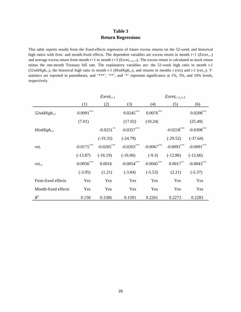
Table 3 reports the regression results. We use two dependent variables, excess return in month
t+1 and average excess return from month t+1 to month t+3, where excess return is calculated as
stock return minus the one-month T-bill rate. We skip one month between excess returns and the
price high ratios to control for the effect of bid-ask bounce. We also add to the regression returns
in months t and t-1 as explanatory variables.
When we regress one-month excess return on the 52-week high ratio in column (1), the
coefficient (0.0091) is significantly positive. This suggests that there is continuation in returns
when a stock price is close to and far from its 52-week high. On the other hand, the coefficient
on the historical high (-0.0251) is significantly negative, providing evidence on return reversals
associated with the nearness to the historical high. These coefficients are robust when we run the
regression with these two anchors together in column (3). We also obtain similar results when we
repeat the regressions using the average three-month excess return in columns (4) to (6). These
results are consistent with George and Hwang (2004) and Li and Yu (2012) in that the nearness
to the 52-week high leads to investors' underreaction and the nearness to the historical high leads
to investors' overreaction. Also, they are in line with Griffin and Tversky (1992), who argue that
individuals tend to underreact to intermittent news but overreact to prolonged news. The results
with the historical high are consistent with Tetlock (2011), who finds strong return reversals
following repeated news.
Overall, the results demonstrate that investors' anchoring behaviors based on the nearness to the
52-week and historical highs lead to different mispricing patterns. A positive relationship
between the nearness to the 52-week high and subsequent returns suggests underreaction
associated with the anchor of the 52-week high, while a negative relationship between the
nearness to the historical high and subsequent returns suggests overreaction associated with the

13
anchor of the historical high. These findings verify the validity of these two price high anchors in
examining short sellers' trading behavior in the next section.
6. Short-Selling Activities and the Nearness to the Past Price Highs
Different return patterns associated with the nearness to the 52-week and historical highs raise
the question of how short sellers exploit information from these past price highs. In Section 3, we
have developed three hypotheses on short sellers’ reaction to the nearness to the 52-week and
historical highs: the behavioral exploitation hypothesis, under which short sellers exploit
investors’ anchoring biases, the contrarian short selling hypothesis, which predicts short sellers’
behavior based on past price levels, and the biased short selling hypothesis, under which short
sellers are subject to the anchoring biases and under- and overreact based on the distances of the
current price to the 52-week and historical highs. As summarized in Table 1, the relationship
between short selling and nearness to these price highs would vary under each hypothesis. Under
the behavioral exploitation hypothesis, short sellers would sell short stocks whose prices are
expected to fall due to investors’ underreaction to bad news and overreaction to good news. Thus,
we expect to find high levels of short-selling activity for stocks whose prices are far from their
52-week highs and close to their historical highs. Meanwhile, if short sellers’ trading strategies
solely rely on past price levels under the contrarian short selling hypothesis, short sellers will
increase their short positions when the stock price is close to these price highs. In the case where
short sellers are subject to the anchoring bias under the biased short selling hypothesis, they will
be reluctant to sell short stocks whose prices are far from the 52-week highs, but they will
increase short-selling activities when the prices are far from the historical highs.
For this analysis, we regress short selling with firm- and month-fixed effects on the lagged
values of nearness to the 52-week and historical highs and other control variables used in prior
studies.
𝑠ℎ𝑡𝑜𝑖,𝑡 = 𝛼 + 𝛽152𝑤𝑘𝐻𝑖𝑔ℎ𝑖,𝑡−1 + 𝛽2𝐻𝑖𝑠𝑡𝐻𝑖𝑔ℎ𝑖,𝑡−1 + 𝛽3𝑟𝑒𝑡𝑖,𝑡 + 𝛽4𝑟𝑒𝑡𝑖,𝑡−1,𝑡−5
+ 𝛽5𝑡𝑢𝑟𝑛𝑜𝑣𝑒𝑟𝑖,𝑡−1 + 𝛽6𝜎𝑖,𝑡−1 + 𝛽7𝐼𝑂𝑖,𝑡−1 + 𝜀𝑡 (1)

14
The dependent variable, shtoi,t, is percentage short turnover for stock i in month t. The key
explanatory variables are 52wkHighi,t-1 and HistHighi,t-1, the measures of the distances of a
stock’s current price to its 52-week and historical highs. The other control variables are: return
for stock i in month t (reti,t), holding-period return from month t-5 to month t-1 (reti,t-1,t-5), trading
volume in month t-1 scaled by total shares outstanding (turnoveri,t-1), price volatility in month t-1
(𝜎𝑖,𝑡−1 ), and institutional ownership (IOi,t-1). Price volatility is calculated as the difference
between the high and low prices in a given month scaled by the high price, and institutional
ownership is the number of shares held by institutions in a given month scaled by total shares
outstanding.
Table 4 summarizes the regression results. Short selling is negatively correlated with the
nearness to the 52-week high in column (1), and the result is robust after we control for return
momentum and other variables in column (2). This suggests that short sellers increase their short
positions when the price is far from the 52-week high and decrease their short positions when the
price is near the 52-week high. On the other hand, short selling is positively associated with the
nearness to the historical high in column (3). That is, short sellers increase their short
transactions when the price is near the historical high, while they decrease their shorting when
the price is far from the historical high. This result is robust when we control for return
momentum and other variables in column (4).
In columns (5) and (6), we estimate the regression model including both price high ratios to
check if the above results still hold. Consistent with the results in columns (1) through (4), short
selling is negatively associated with the nearness to the 52-week high, while it is positively
associated with the nearness to the historical high. Since the signs of the coefficients on the 52-
week and historical high ratios are opposite, it is unlikely that the effects of the 52-week and
historical highs are driven by each other. These results clearly confirm short sellers' different
behavior with respect to the nearness to the 52-week and historical highs.
The results in Table 4 support the behavioral exploitation hypothesis: short sellers exploit
underreaction associated with the 52-week high and overreaction associated with the historical
high. This suggests that short sellers are able to identify relative price levels that lead to under-
and overreaction. Moreover, these findings show that short sellers do not simply base their trades
on past price levels, and they are not subject to an anchoring bias.

15
The results in columns (2), (4), and (6) also suggest the relationship between short selling and
other variables. The relationship between short selling and contemporaneous returns is in general
insignificant, but short selling is negatively associated with past returns. This is different from
contrarian patterns in prior studies. As discussed above, we use the ratios of the stock price to the
52-week and historical highs as proxies for under- and overreaction separately, while prior
studies use past returns as a proxy for overreaction. Given this, we presume that our proxies
capture short-selling behavior based on investors' under- and overreaction, leading us to fail to
find a positive correlation between shorting and past returns.
Also, short selling is positively correlated with turnover and institutional ownership, which is
consistent with prior studies. In particular, since institutional ownership has been used as a proxy
for short sale constraints, the positive association between short selling and institutional
ownership confirms more short-selling activities for stocks that are less short sale constrained.
In conclusion, we find evidence in favor of the behavioral exploitation hypothesis. Neither are
short sellers subject to the anchoring biases nor do their short-selling activities simply increase
with the distances of the current price to the past price highs. Rather, they are able to exploit
underreaction to bad news when the stock price is far from its 52-week high and overreaction to
good news when the price is close to the historical high.15
Based on these findings, we expect
that such short-selling behavior will affect the degree of mispricing and return patterns
associated with the 52-week and historical highs. This will be discussed in the following section.
7. The Impact of Short-Selling Activities on Future Return Patterns
We find above that short sellers are able to trade on underreaction to bad news and overreaction
to good news when the current price is far from the 52-week high and close to the historical high.
These findings lead us to question the possible impact of such short-selling behavior on
subsequent returns. When the price is far from the 52-week high, investors underreact to bad
news and such underreaction leads to downward momentum in stock returns. If short sellers
trade on this underreaction actively, stocks with high short selling will tend to have weaker
15
The profitability of short-selling strategies based on other investors' irrationality depends on when short sellers
unwind their short positions, which is not available in our short interest data.

16
return momentum compared to those with low short selling. In the same vein, when the stock
price is close to its historical high, investors tend to overreact to good news and such
overreaction leads to downward price reversals. If short sellers enter their short positions by
exploiting this overreaction, stocks with high short-selling activities will tend to have weaker
reversals compared to those with low short-selling activities.
In order to examine this, we sort stocks into quintiles based on the nearness to the 52-week and
historical highs in month t-1 and then, within each quintile, sort the stocks into five portfolios
based on short turnover in month t. For each 5× 5 portfolio, we calculate average excess and
abnormal returns over the subsequent 6 and 12 months.16
The excess return is calculated as the
actual stock return minus the one-month T-bill rate, and the abnormal return is calculated as the
difference between stock return and an equal-weighted market index return.17
Table 5 reports the average excess and abnormal returns for stocks whose prices are farthest
from their 52-week highs (Q1) and whose prices are nearest to the historical highs (Q5). We
focus our analysis on these two portfolios, because short sellers trade actively in these portfolios
by exploiting underreaction to bad news and overreaction to good news. Panel A reports the
excess and abnormal returns for stocks whose prices are farthest from the 52-week highs. While
lightly shorted stocks have lower subsequent excess and abnormal returns, heavily shorted stocks
have relatively higher excess and abnormal returns. Differences in returns between the lightly
and heavily shorted portfolios (Q1-Q5) are significantly negative, although the differences in 6-
month excess returns are marginally significant. These results are in line with our prediction that
high short-selling activities for stocks whose prices are far from the 52-week highs attenuate
continuations of past returns, enhancing market quality.
Panel B reports the average excess and abnormal returns for stocks whose prices are nearest their
historical highs. Similar to the above, the lightly shorted portfolio has lower subsequent returns
than the heavily shorted portfolio, and the return differences between the two shorted portfolios
(Q1-Q5) are significantly negative. In particular, abnormal 6-month and 1-year returns for the
heavily shorted portfolio are positive, while those for the lightly shorted portfolio are negative.
16
As in Table 3, we skip one month between portfolio formation and holding periods to control for the effect of bid-
ask bounce. 17
We also run the tests using abnormal returns calculated as the difference between stock returns and value-
weighted market index returns, but the results are unchanged.
17
This suggests that return reversals even disappear if short sellers trade actively on overreaction
when the stock price is close to the historical high.
Overall, the results show that short-selling activities based on the nearness to the 52-week and
historical highs reduce mispricing driven by investors' anchoring biases. These findings suggest
that short sellers’ tendency to take advantage of other investors’ irrational behavior helps
improve the price discovery process.
8. Additional Tests
8.1. How Short Sellers React when the 52-Week is Equal to the Historical Highs?
We have shown that the distances of the current price to the 52-week and historical highs lead to
different patterns in future returns and short sellers' trading behavior. The nearness to the 52-
week high is positively associated with future returns, while the nearness to the historical high is
negatively associated with future returns. Short sellers benefit from these mispricing patterns by
increasing their short positions when the stock price is far from its 52-week high and close to its
historical high. For these analyses, we have excluded stocks whose 52-week highs equal their
historical highs, because the same levels of the 52-week and historical highs do not indicate the
degree of bad or good news and thus do not proxy for investors' under- or overreaction. In
addition, the stock price can reach its historical high without prolonged good news, since it has
an increasing trend over time. In this case, the nearness to the historical high would be the same
proxy as the nearness to the 52-week high.18
When the 52-week high equals the historical high,
we would expect to find a positive association between the nearness to the price high and
subsequent returns and a negative association between the nearness to the price high and short
selling.
To examine this, we repeat all the analyses for stocks whose 52-week highs equal their historical
highs.19
We first regress future (1-month and 3-month) excess returns on the nearness to the past
price high ratio and returns in months t and t-1 with firm- and month-fixed effects. Panel A of
Table 6 reports the coefficient estimate on the past price high ratio from the regression. The
18
Since the 52-week high equals the historical high, we refer to this as the (past) price high in this section. 19
About 28% of observations have the same 52-week and historical highs.

18
coefficient on the nearness to the price high is significantly positive, suggesting that there are
continuations of the past returns when the 52-week high equals the historical high. This confirms
that investors tend to underreact in this case and the nearness to the historical high does not
proxy for overreaction or prolonged news.
Panel B reports results from the regression of short turnover on the nearness to the price high.
Contrary to our expectations and the findings in Table 4, the coefficient on the nearness to the
past price high is significantly positive in column (1), and its magnitude is even larger when we
add other control variables in column (2). This shows that short selling tends to increase with the
nearness to the past price high when the 52-week high equals the historical high. This provides
evidence against informed short selling. Short sellers fail to exploit other investor's anchoring
bias when the 52-week high equals the historical high.
If the stock price is close to the same 52-week and historical highs, short sellers may place much
weight on the fact that the price is approaching both of the price highs and expect downward
return reversals. In this case, even if there are informed short sellers who trade on underreaction,
it appears that their behavior will be dominated by trading behavior of uninformed short sellers.
Therefore, this result does not support that short sellers trade on their information advantage.
Related to this, we further examine if the shorting patterns found above affect return
continuations associated with the price high. In unreported results, we find insignificant
differences in future returns between lightly and heavily shorted portfolios, and the finding is
robust to different types of returns (excess and abnormal returns) or holding periods of returns.
This may provide a clue to the effect of uninformed short-selling activities when the 52-week
high equals the historical high.
Overall, we do not find that short sellers exploit investors' underreaction when the 52-week high
equals the historical high. Such short-selling activities do not contribute to market quality by
weakening return momentum and improving price discovery.
8.2. Non-January and January months
Since we use monthly data to examine return patterns linked to the 52-week and historical highs,
we examine if our results are robust to seasonal anomalies, such as the January effect. We divide
the sample into non-January and January data and rerun the regressions shown in Tables 3 and 4.
Table 7 summarizes the regression results for non-January and January months. Panel A shows

19
that, although the positive relationship between future returns and the nearness to the 52-week
high is less significant in January, the overall results confirm the existence of return momentum
and reversals associated with the 52-week and historical highs in both subsamples. In Panel B,
we find that short-selling activities related to the nearness to these two anchors are also
consistent with our findings in Table 4, although the negative coefficient on the nearness to the
52-week high and the positive coefficient on the nearness to the historical high are less
significant in January than those for non-January months. In summary, our results on the 52-
week and historical highs are robust to return patterns associated with seasonal anomalies such as
the January effect.
9. Conclusions
We examine if nearness of a stock price to its 52-week or historical high affects short-selling
behavior in the equity market. We first confirm that future returns are positively correlated with
the nearness to the 52-week high and negatively correlated with the nearness to the historical
high. This finding indicates that investors tend to underreact when the price is near or far from
the 52-week high, while they tend to overreact when the price is near or far from the historical
high. Using these two proxies for investors' under and overreaction, we find that short selling is
negatively associated with the nearness to the 52-week high and positively associated with the
nearness to the historical high. This suggests that short sellers tend to increase short positions
when the stock price is far from its 52-week high and near its historical high, and they decrease
their shorting when the price is near the 52-week high and far from the historical high. Linking
these findings to the return patterns associated with the 52-week and historical highs, we can
conclude that short sellers exploit underreaction to bad news when the price is far from the 52-
week high and overreaction to good news when the price is near the historical high. We also find
that stocks with high short-selling activity exhibit weaker return momentum and reversals when
the stock price is far from the 52-week high and close to the historical high. This shows that
short sellers' behavior of exploiting investors' anchoring biases contributes to correcting
mispricing quickly and enhancing price discovery.

20
Our results are robust in subsamples for January and non-January months. However, when the
52-week high equals the historical high, we do not find evidence that short sellers exploit
underreaction to bad news. Overall, the results show that short sellers exploit other investors'
anchoring biases associated with the 52-week and historical highs. They trade on underreaction
to bad news when the stock price is far from the 52-week high, and they trade on overreaction to
good news when the price is close to the historical high. Neither are they subject to anchoring
biases nor do their trading activities solely depend on recent price levels relative to the past price
highs. Our results are consistent with the prevailing view in the field of behavioral finance that
rational and sophisticated traders are less susceptible to behavioral biases.

21
References
Andreassen, P., 1987, On the social psychology of the stock market: Aggregate attributional
effects and the regressiveness of prediction, Journal of Personality and Social Psychology 53,
490-496.
Andreassen, P., 1988, Explaining the price-volume relationship: The difference between price
changes and changing prices, Organizational Behavior and Human Decision Processes 41, 371-
389.
Asquith, P., P. A. Pathak, and J. R. Ritter, 2005, Short interest, institutional ownership, and stock
returns, Journal of Financial Economics 78, 243-276.
Baker, M., X. Pan, and J. Wurgler, 2012, The effect of reference point prices on mergers and
acquisitions, Journal of Financial Economics 106, 49-71.
Barberis, N., and W. Xiong, 2009, What drives the disposition effect? An analysis of a long-
standing preference-based explanation, Journal of Finance 64, 751-784.
Beschwitz, B., and M. Massa, 2013, Biased shorts: stock market implications of short sellers'
disposition effect, working paper, INSEAD.
Boehmer, E., Z. R. Huszar, and B. D. Jordan, 2010, The good news in short interest, Journal of
Financial Economics 96, 80-97.
Boehmer, E., and J. Wu, 2013, Short selling and the price discovery process, Review of Financial
Studies 26, 287-322.
Campbell, S., and S. Sharpe, 2009, Anchoring bias in consensus forecasts and its effect on
market prices, Journal of Financial and Quantitative Analysis 44, 369-390.
Cen, L., H. Gilles, and K. Wei, 2013, The role of anchoring bias in the equity market: Evidence
from analysts' earnings forecasts and stock returns, Journal of Financial and Quantitative
Analysis 48, 47-76.
Christophe, S. E., M. G. Ferri, and J. J. Angel, 2004, Short-selling prior to earnings
announcements, Journal of Finance 59, 1845-1875.
Christophe, S. E., M. G. Ferri, and J. Hsieh, 2010, Informed trading before analyst downgrades:
Evidence from short sellers, Journal of Financial Economics 95, 85-106.
Dechow, P. M., A. P. Hutton, L. Meulbroek, and R. G. Sloan, 2001, Short-sellers, fundamental
analysis, and stock returns, Journal of Financial Economics 61, 77-106.
Degeorge, F., J. Patel, and R. Zeckhauser, 1999, Earnings management to exceed thresholds,
Journal of Business 72, 1-33.

22
De Long, B., A. Shleifer, L. Summers, and R. Waldmann, 1990, Noise trader risk in financial
markets, Journal of Political Economy 98, 703-738.
Desai, H., S. Krishnamurthy, and K. Venkataraman, 2006, Do short-sellers target firms with poor
earnings quality? Evidence from earnings restatements, Review of Accounting Studies 11, 71-90.
Diether, K. B., K. H. Lee, and I. M. Werner, 2009, Short-sale strategies and return predictability,
Review of Financial Studies 22, 575-607.
Du, D., 2008, The 52-week high and momentum investing in international stock indexes,
Quarterly Review of Economics and Finance 48, 61-77.
Engelberg, J. E., A. V. Reed, and M. C. Ringgenberg, 2012, How are shorts informed? Short
sellers, news, and information processing, Journal of Financial Economics 105, 260-278.
Feng, L., and M. S. Seasholes, 2005, Do investor sophistication and trading experience eliminate
behavioral biases in financial markets? Review of Finance 9, 305-351.
George, T., and C. Y. Hwang, 2004, The 52-week high and momentum investing, Journal of
Finance 59, 2145-2175.
Griffin, D., and A. Tversky, 1992, The weighing of evidence and the determinants of confidence.
Cognitive Psychology 24, 411-435.
Grinblatt, M., and B. Han, 2005, Prospect theory, mental accounting, and momentum, Journal of
Financial Economics 78, 311-339.
Grinblatt, M., and M. Keloharju, 2001, What makes investors trade? Journal of Finance 51, 589-
616.
Heath, C., S. Huddart, and M. Lang, 1999, Psychological factors and stock option exercise,
Quarterly Journal of Economics 114, 601-627.
Henry, T. R., D. J. Kisgen, and J. Wu, 2014, Equity short selling and bond rating downgrades,
Journal of Financial Intermediation, Forthcoming
Henry, T. R., and J. L. Koski, 2010, Short selling around seasoned equity offerings, Review of
Financial Studies 23, 4389-4418.
Hong, X., B. D. Jordan, and M. H. Liu, 2012, Industry information and the 52-week high effect,
Working paper, University of Kentucky.
Huddart, S., M. Lang, and M. H. Yetman, 2009, Volume and price patterns around a stock’s 52-
week highs and lows: theory and evidence, Management Science 55, 16-31.

23
Kahneman, D., and A. Tversky, 1973, On the Psychology of Prediction, Psychological Review
80, 237–251.
Kahneman, D., and A. Tversky, 1979, Prospect theory: An Analysis of decisions under risk,
Econometrica 47, 313-327.
Karpoff, J., and X. Lou, 2010, Short sellers and financial misconduct, Journal of Finance 65,
1879-1913.
Kelly, E., and P. Tetlock, 2013, Retail Short Selling and Stock Prices, Columbia Business School
Research Paper No. 13-70.
Li, J., and J. Yu, 2012, Investor attention, psychological anchors, and stock return predictability,
Journal of Financial Economics 104, 401-419.
Ljungqvist, A., and W. Wilhelm, 2005, Does prospect theory explain IPO market behavior?
Journal of Finance 60, 1759-1790.
Loughran, T., and J. Ritter, 2002, Why don't issuers get upset about leaving money on the table
in IPOs? Review of Financial Studies 15, 413-444.
Poteshman, A., and V. Serbin, 2003, Clearly irrational financial market behavior: Evidence from
the early exercise of exchange traded stock options, Journal of Finance 58, 37-70.
Shefrin, H. M., and M. Statman, 1985. The disposition to sell winners too early and ride losers
too long: theory and evidence. Journal of Finance 40, 777-790.
Tetlock, P. C., 2011, All the news that's fit to reprint: Do investors react to stale information?
Review of Financial Studies 23, 3520-3557.
Tversky, A., and D. Kahneman, 1971, Belief in the Law of Small Numbers, Psychological
Bulletin 76, 105–110.
Tversky, A., and D. Kahneman, 1974, Judgment under uncertainty: Heuristics and biases,
Science 185, 1124-1131.
Watson, E., and M. Funck, 2012, A cloudy day in the market: short selling behavioral bias or
trading strategy, International Journal of Managerial Finance 8, 238-255.

24
Table 1
Predictions of Short Selling on the Nearness to the 52-Week and Historical Highs
This table describes levels of short selling under three possible hypotheses explained in Section 3. The first
hypothesis is the behavioral exploitation hypothesis, which represents trading behavior of sophisticated short sellers
who can exploit other investors' behavioral biases. The second hypothesis is the contrarian short selling hypothesis,
which indicates high levels of short sales following a price rise. The third hypothesis is the biased short selling
hypothesis, which indicates that short sellers are subject to anchoring biases and under- and overreact to bad news.
Nearness to the 52-week high Nearness to the historical high
Nearest Farthest Nearest Farthest
Behavioral exploitation Low High High Low
Contrarian short selling High Low High Low
Biased short selling - Low - High

25
Table 2
Descriptive Statistics
This table reports the time-series averages of the cross-sectional means for stock-level variables of NYSE, AMEX,
and NASDAQ common stocks from 1995 through 2012. 52wkHigh is the ratio of monthly price divided by the
highest price achieved within the past 52 weeks, and HistHigh is the ratio of the monthly price scaled by the highest
price in the history. vol is the number of shares traded over a month, and turnover is monthly trading volume scaled
by the number of shares outstanding. ret is monthly return, mcap is the logarithm of the market value of equity
calculated as monthly stock price times the number of shares outstanding, and bm is the book value of equity (book
value of stockholder’s equity plus balance sheet deferred taxes minus the book value of preferred stock) divided by
the market value of equity. σ is the difference between the high and low prices during month t scaled by the high
price, and IO is the number of shares held by institutional investors, scaled by total shares outstanding. Short interest
is the number of shorted shares outstanding as of the 15th
day of each month, and shto is short interest scaled by total
shares outstanding.
Mean Std Quartile 1 Median Quartile 3
52wkHigh (%) 82.19 7.78 77.57 84.4 87.33
HistHigh (%) 47.11 4.82 43.96 46.81 50.2
vol (in millions) 16.00 9.52 6.75 15.42 23.67
turnover (%) 13.18 5.69 7.32 14.18 17.63
ret (%) 1.8 5.11 -1 2.16 4.8
mcap 20.13 0.21 19.99 20.08 20.28
bm (%) 61.68 10.68 51.21 60.78 68.87
σ (%) 13.34 3.43 11.21 12.33 14.31
IO (%) 56.94 11.12 48.97 57.95 64.19
Short interest (in millions) 3.33 1.17 2.22 3.18 4.33
shto (%) 4.54 1.47 3.39 4.42 5.48
26
Table 3
Return Regressions
This table reports results from the fixed-effects regression of future excess returns on the 52-week and historical
high ratios with firm- and month-fixed effects. The dependent variables are excess return in month t+1 (Exrett+1)
and average excess return from month t+1 to month t+3 (Exrett+1,t+3). The excess return is calculated as stock return
minus the one-month Treasury bill rate. The explanatory variables are: the 52-week high ratio in month t-1
(52wkHight-1), the historical high ratio in month t-1 (HistHight-1), and returns in months t (rett) and t-1 (rett-1). T-
statistics are reported in parentheses, and ‘***’, ‘**’, and ‘*’ represent significance at 1%, 5%, and 10% levels,
respectively.
Exrett+1 Exrett+1,t+3
(1) (2) (3) (4) (5) (6)
52wkHight-1 0.0091***
0.0245***
0.0076***
0.0208***
(7.01)
(17.02) (10.24) (25.49)
HistHight-1
-0.0251**
-0.0357***
-0.0218***
-0.0308***
(-19.33) (-24.79) (-29.52) (-37.64)
rett -0.0175***
-0.0205***
-0.0203***
-0.0067***
-0.0093***
-0.0091***
(-13.87) (-16.19) (-16.06) (-9.3) (-12.86) (-12.66)
rett-1 -0.0056***
0.0016 -0.0054***
-0.0045***
0.0017**
-0.0043***
(-3.95) (1.21) (-3.84) (-5.53) (2.21) (-5.37)
Firm-fixed effects Yes Yes Yes Yes Yes Yes
Month-fixed effects Yes Yes Yes Yes Yes Yes
R2 0.158 0.1586 0.1591 0.2261 0.2273 0.2283

27
Table 4
Short-Selling Regressions
This table reports results from the fixed-effects regressions of short turnover on the 52-week high ratio, the historical
high ratio, and other control variables with firm- and month-fixed effects. The dependent variable is short turnover
in month t (shtot). The explanatory variables are: the 52-week high ratio in month t-1 (52wkHight-1), the historical
high ratio in month t-1 (HistHight-1), stock return in month t (rett), holding-period return from month t-5 to month t-
1 (rett-1,t-5), turnover in month t-1 (turnovert-1), price volatility in month t-1 (σt-1), and institutional ownership in
month t-1 (IOt-1). The 5-day holding period return is calculated as the percentage change in price from the last price
in month t-6 to the last price in month t-1. T-statistics are reported in parentheses, and ‘***’, ‘**’, and ‘*’ represent
significance at 1%, 5%, and 10% levels, respectively.
(1) (2) (3) (4) (5) (6)
52wkHight-1 -2.1134***
-1.3491***
-3.2805***
-1.9091***
(-28.26) (-15.23)
(-38.99) (-19.6)
HistHight-1
1.051***
0.5258***
2.6038***
1.2888***
(13.66) (6.19) (30.11) (13.79)
rett
-0.003
0.1487* 0.1041
(-0.03)
(1.69) (1.18)
rett-1,t-5
-0.1414***
-0.327***
-0.1356***
(-5.58)
(-13.99) (-5.36)
turnovert-1
2.095***
2.0958***
2.0534***
(103.26)
(102.71) (100.14)
𝜎𝑖,𝑡−1
-2.1841***
-1.338***
-1.9248***
(-11.49)
(-7.09) (-10.08)
IOt-1
0.0094***
0.0094***
0.0092***
(2.99)
(2.99) (2.92)
Firm-fixed effects Yes Yes Yes Yes Yes Yes
Month-fixed effects Yes Yes Yes Yes Yes Yes
R2 0.5063 0.5389 0.5053 0.5386 0.5077 0.5392

28
Table 5
Subsequent Returns for Shorted Portfolios
This table reports the average excess and abnormal returns for portfolios sorted on the 52-week or historical high
ratio in month t-1 and short selling in month t. We sort stocks into quintile portfolios by the 52-week or historical
high ratio in month t-1 and, with each group, sort the stocks into five portfolios based on short turnover in month t.
Panel A presents 6-month ([+2,+7]) and 12-month ([+2,+13]) excess and abnormal returns for the portfolio that is
farthest from the 52-week high (Q1), and Panel B reports the excess and abnormal returns for the portfolio that is
nearest the historical high (Q5). Q1 and Q5 in the first column of each table indicate the lightly and heavily shorted
portfolios. The excess return is calculated as stock return minus the one-month T-bill rate. The abnormal return is
the difference between stock return and equal-weighted market index return. T-statistics are reported in parentheses,
and ‘***’, ‘**’, and ‘*’ represent significance at 1%, 5%, and 10% levels, respectively.
Panel A. Stocks whose prices are farthest from the 52-week highs (Q1)
Excess returns (%) Abnormal returns (%)
[+2, +7] [+2, +13] [+2, +7] [+2, +13]
Q1 (Lightly shorted) 0.2249 0.3425 -0.4847 -0.3562
Q5 (Heavily shorted) 0.3982 0.5365 -0.3068 -0.1459
Diff. (Q1-Q5) -0.1733* -0.194
*** -0.1779
** -0.2103
***
(-1.85) (-2.58) (-2.09) (-3)
Panel B. Stocks whose prices are nearest the historical highs (Q5)
Excess returns (%) Abnormal returns (%)
[+2, +7] [+2, +13] [+2, +7] [+2, +13]
Q1 (Lightly shorted) 0.5294 0.4795 -0.1861 -0.218
Q5 (Heavily shorted) 0.9951 1.0148 0.2893 0.3158
Diff. (Q1-Q5) -0.4657***
-0.5353***
-0.4754***
-0.5338***
(-7.64) (-10.87) (-8.03) (-11.08)

29
Table 6
Regressions with the Same 52-Week and Historical Highs
This table reports results from the fixed-effects regressions of future returns and short selling on the nearness to the
past price high with firm- and month-fixed effects when the 52-week high equals the historical high. We first regress
future (1-month and 3-month) excess returns on the nearness to the past price high ratio and returns in months t and
t-1. Panel A reports the coefficient estimate on the past price high ratio from the regression. Panel B reports the
regression results of short turnover on the price high ratio in month t-1 (Hight-1), return in month t (rett), holding-
period return from month t-5 to month t-1 (rett-1,t-5), turnover in month t-1 (turnovert-1), price volatility in month t-1
(σt-1), and institutional ownership in month t-1 (IOt-1). T-statistics are reported in parentheses, and ‘***’, ‘**’, and ‘*’
represent significance at 1%, 5%, and 10% levels, respectively.
Panel A. Subsequent returns
Exrett+1 Exrett+1,t+3
Hight-1 0.0177***
0.0135***
(8.57) (11.94)
Panel B. Short turnover
(1) (2)
Hight-1 0.4112***
1.7242***
(3.09) (10.75)
rett
0.1288
(0.73)
rett-1,t-5
-0.1507***
(-3.84)
turnovert-1
1.7128***
(44.03)
𝜎𝑖,𝑡−1
-4.5461***
(-14.19)
IOt-1
5.8025***
(41.22)
Firm-fixed effects Yes Yes
Month-fixed effects Yes Yes
R2 0.6165 0.6882

30
Table 7
Regressions for Non-January and January Months
This table reports results from the fixed-effects regressions of future returns and short selling on the nearness to the
52-week and historical highs for non-January and January months. We separate the entire sample into two
subsamples, non-January and January months. Panel A reports the coefficient estimates on the 52-week and
historical high ratios from the regression of future 1-month excess returns on the 52-week and historical high ratios
in month t-1 (Hight-1) and returns in months t (rett) and t-1 (rett-1). In Panel B, we regress short turnover on the 52-
week and historical high ratios in month t-1 (Hight-1), return in month t (rett), holding-period return from month t-5
to month t-1 (rett-1,t-5), turnover in month t-1 (turnovert-1), price volatility in month t-1 (σt-1), and institutional
ownership in month t-1 (IOt-1). T-statistics are reported in parentheses, and ‘***’, ‘**’, and ‘*’ represent
significance at 1%, 5%, and 10% levels, respectively.
Panel A. Subsequent 1-month excess returns
Non-January January
52wkHight-1 0.0271***
0.0127**
(18.12) (2.35)
HistHight-1 -0.0329***
-0.0544***
(-22.05) (-10.06)
Panel B. Short turnover
Non-January January
52wkHight-1 -1.957***
-0.6484*
(-19.08) (-1.67)
HistHight-1 1.2973***
0.8315**
(13.16) (2.44)
rett 0.1149 0.1721
(1.24) (0.47)
rett-1,t-5 -0.122***
-0.3068**
(-4.65) (-2)
turnovert-1 2.0767***
1.7537***
(95.86) (22.61)
𝜎𝑖,𝑡−1 -1.9032***
-0.9646***
(-9.41) (-1.34)
IOt-1 0.0086***
5.0813***
(2.71) (16.33)
Firm-fixed effects Yes Yes
Month-fixed effects Yes -
R2 0.5375 0.5543
Top Related