
![Characterization of Langmuir-Blodgett Films of a Calix[8]Arene and Sensing Properties](https://static.fdocuments.us/doc/165x107/577d24041a28ab4e1e9b660a/characterization-of-langmuir-blodgett-films-of-a-calix8arene-and-sensing.jpg)


Languages
Pages
Legal

Departamento de Química-Física
Facultad de Ciencias Químicas
SSSEEELLLFFF---AAASSSSSSEEEMMMBBBLLLEEEDDD SSSYYYSSSTTTEEEMMMSSS OOOFFFNNNAAANNNOOOMMMAAATTTEEERRRIIIAAALLLSSS OOONNN
LLLAAANNNGGGMMMUUUIIIRRR---BBBLLLOOODDDGGGEEETTTTTT FFFIIILLLMMMSSS
SSSiiisssttteeemmmaaasss AAAuuutttooo---eeennnsssaaammmbbblllaaadddooosss dddeee NNNaaannnooommmaaattteeerrriiiaaallleeesss eeennnPPPeeelllííícccuuulllaaasss LLLaaannngggmmmuuuiiirrr---BBBlllooodddgggeeetttttt
BBBeeeaaatttrrriiizzz MMMaaarrrtttííínnn GGGaaarrrcccíííaaa
SSSaaalllaaammmaaannncccaaa 222000111333

FACULTAD DE CIENCIAS QUÍMICAS
Departamento de Química-Física
SELF-ASSEMBLED SYSTEMS OF NANOMATERIALS ON
LANGMUIR-BLODGETT FILMS
SISTEMAS AUTOENSAMBLADOS DE NANOMATERIALES EN PELÍCULAS LANGMUIR-BLODGETT
BEATRIZ MARTÍN GARCÍA
Salamanca, 2013


FACULTAD DE CIENCIAS QUÍMICAS
Departamento de Química-Física
SELF-ASSEMBLED SYSTEMS OF NANOMATERIALS ON LANGMUIR-BLODGETT FILMS
SISTEMAS AUTOENSAMBLADOS DE NANOMATERIALES EN
PELÍCULAS LANGMUIR-BLODGETT
Memoria que para optar al grado de Doctor por la Universidad de Salamanca presenta la licenciada Beatriz Martín García
Salamanca, 15 de Abril de 2013
Fdo. Beatriz Martín García


Dª. Mª Mercedes Velázquez Salicio, Catedrática de Universidad en el
Departamento de Química-Física de la Universidad de Salamanca,
INFORMA:
Que el trabajo presentado como Tesis Doctoral por la licenciada en Ingeniería
Química Beatriz Martín García para optar al grado de Doctor por la Universidad
de Salamanca, titulado "Self-assembled Systems of Nanomaterials on
Langmuir-Blodgett Films / Sistemas Auto-ensamblados de
Nanomateriales en Películas Langmuir-Blodgett" ha sido realizado en el
laboratorio del G.I.R de Coloides e Interfases en el Dpto. Química-Física de la
Facultad de Ciencias Químicas de la Universidad de Salamanca (España) y en las
instalaciones del Grupo de Fotoquímica Molecular del Instituto Superior Técnico
de Lisboa (Portugal).
Como directora del trabajo, autoriza la presentación del mismo, al considerar que
se han alcanzado los objetivos marcados.
Y para que conste, firmo el presente en Salamanca a 15 de Abril de 2013.
Fdo. Mª Mercedes Velázquez Salicio


El trabajo que engloba la presente Memoria se ha realizado durante el
periodo de disfrute de una Beca de Colaboración (curso 2006/2007) en el
Departamento de Química-Física del Ministerio de Educación y Ciencia y una
ayuda a la contratación de Personal Investigador de Reciente Titulación
Universitaria (2008/2012) de la Junta de Castilla y León concedida al amparo de la
Orden EDU/330/2008 de 3 de marzo.
El trabajo desarrollado dentro del G.I.R. de Coloides e Interfases del
Departamento de Química-Física ha sido financiado por los proyectos: MAT
2004-04180, MAT 2007-62666 y MAT 2010-19727 del Ministerio de Educación y
Ciencia; y SA038A05 y SA038A08 de la Junta de Castilla y León.


ʺI am among those who think that science has great beauty.
A scientist in his laboratory is not only a mere technician:
he is also a child confronting natural phenomena
which impress him like a fairy taleʺ
by Marie Sklodowska Curie


Acknowledgments
En estas líneas quiero expresar mi agradecimiento a todas aquellas personas que de una
manera u otra han intervenido en el desarrollo del presente trabajo y por tanto, lo han hecho
posible. Espero no olvidarme de nadie, pero por si acaso, pido disculpas por anticipado.
Agradecerles su compañía en esta difícil tarea y su ayuda a crecer como persona tanto humana y
como científicamente.
En primer lugar quisiera agradecer a mi Directora, Prof. Dra. Dª. Mercedes
Velázquez Salicio, por brindarme la oportunidad de introducirme en el mundo de la
investigación dentro del Grupo de Coloides e Interfases de la Universidad de Salamanca y
transmitirme cada día su ilusión por este trabajo. Así como su inestimable ayuda en el trabajo
de cada día y en la elaboración de esta memoria.
Dentro del Departamento de Química-Física, quisiera agradecer también a la Prof.
Dra. Dª. Mª Dolores Merchán Moreno el apoyo y los consejos recibidos durante este tiempo.
También hacer un especial agradecimiento a los Prof. Drs. José Luis Usero, Mª Ángeles del
Arco, Carmen Izquierdo, Julio Casado y Emilio Calle, por su colaboración en determinados
momentos.
Al Dpto. de Química Orgánica, en especial a los Prof. Drs. D. Francisco Bermejo y
Dª. Josefa Anaya por su asesoramiento en síntesis; y al Prof. Dr. Joaquín R. Morán por
compartir su sabiduría a la hora resolver cuestiones puntuales sobre productos y disolventes. Al
Dpto. de Química Inorgánica, concretamente a Prof. Drs. D. Vicente Rives y Dª. Raquel
Trujillano por su disponibilidad y facilidades para utilizar varios equipos. Al Dpto. de
Bioquímica y Biología Molecular, en especial a la Prof. Dra. Dª. Nieves Pérez por su
amabilidad y accesibilidad para el uso de las centrífugas. Al Servicio de Microscopía, con
mención a sus técnicos Juan y en los últimos tiempos, a Marta por su fantástica predisposición.
Al Dpto. de Química Analítica, por las pruebas en las centrífugas, algunos compuestos químicos
y el agua cuando fallaba el MilliQ, y sobre todo como ellos dicen por salvarme la "vida". Al

CLPU y todo su equipo por facilitar la realización de las medidas de AFM, pero con especial
hincapié en José y Juan, por su paciencia y dedicación.
Y continuando con la Física, al Prof. Dr. D. Enrique Diez y su doctorando, Cayetano
S. Cobaleda, del Laboratorio de Bajas Temperaturas (Universidad de Salamanca) por
adentrarme en el mundo del grafeno. In questa linea, vorrei anche ringraziare il Prof. Dr.
Vittorio Bellani ed il Dr. Francesco Rosella (Università di Pavia, Italia) per la loro
inestimabile collaborazione ed il loro appoggio. Aquí, también me gustaría dedicar unas
palabras de agradecimiento a la gente del ISOM-UPM, en especial a Mª Mar, David, Maika,
Alicia y José Antonio. Al Grupo de Dispositivos Semiconductores (Universidad de Salamanca),
en especial al Prof. Drs. D. Tomás González y al D. Ignacio Íñiguez de la Torre, por hacer
posibles las medidas de conductividad y su dedicación.
Al Grupo de Sistemas Complejos de la Universidad Complutense de Madrid (UCM),
en especial a los Prof. Drs. Francisco Ortega y Ramón G. Rubio por darme la oportunidad de
realizar una estancia en el grupo y permitir el acceso al uso del elipsómetro, y al Dr. José E.F.
Rubio por las medidas. Destacar la fantástica acogida y las charlas con Eduardo, Armando,
Hernán, Marta y Mónica. También al Prof. Dr. D. Valentín García Baonza de la UCM,
por algunas pruebas de Espectroscopía Raman.
Asimismo, agradecer a la Prof. Dra. Dª. Margarita González Prolongo y a su equipo
del Departamento de Materiales y Producción Aeroespacial de la Escuela Técnica Superior de
Ingenieros Aeronáuticos de la Universidad Politécnica de Madrid (UPM) por permitirnos
utilizar el equipo de Calorimetría Diferencial de Barrido (DSC).
Al Prof. Dr. José Luis G. Fierro del Instituto de Catálisis y Petroquímica (CSIC),
por su colaboración y discusiones de las medidas de XPS. Al Prof. Dr. Albert Cicera y a Sergi
Claramunt del Departmento de Electrónica de la Universitat de Barcelona, por facilitar la
realización de las medidas de FE-SEM.
À Professora Silvia M.B. Costa, do Instituto Superior Tecnico da Lisboa, pela
oportunidade de fazer uma estadia no seu grupo de investigação, a sua implicação no
desenvolvimento do trabalho, preocupação e atenções. Também por deixa-me participar nas
reuniões do grupo, como um membro mais, e poder apresentar e discutir o nosso trabalho. Ao

Dr. Pedro M.R. Paulo pela sua dedicação, ajuda, ensinamentos e longas discussões dos
resultados durante e depois da minha estadia. Com licença e hulmidade, gostaria de poder lhes
dedicar o capitulo da tese da fotofísica dos quantum dots, onde agradeço a ajuda na elabora
redacção ao Dr. Pedro M.R. Paulo. Muito obrigada também à tudos os membros do Grupo de
Fotoquímica Molecular pelo trato recibido durante a minha estadia.
Para el final querría hacer un punto de inflexión, para agradecer los momentos
divertidos y de apoyo de los que considero mis compañeros y mis amigos. Primeramente, a Teresa,
con la que empecé mi andadura en el doctorado y con la que he tenido la oportunidad de trabajar
y compartir buenos y malos momentos, estancias y congresos, un gran apoyo y amiga, simplemente
gracias. A mis "asesores"... por el apoyo y los sabios consejos. A mis amigos, por las velas, las
oraciones y la confianza en mí. Por lo importante que ha sido el entorno de trabajo, a mis
compañeros de laboratorio, David, Rubén y Sofía. A los compañeros de Departamento, tanto a
los que están como a los que afortunadamente han encontrado un post-doc o trabajo, por hacer
más ameno el día a día, el paintball, las discusiones científicas y conseguir artículos, Pablo, Jesús,
Susana, Marina, Jorge, Mario, Rafa, Fabián, Manso, Teresa, Jessica, Nico y Ruth. Sin
poderme olvidar tampoco de los orgánicos de Villarriba en especial de Ángel, gracias por todo,
aquí incluiré también a Sole y a Juan, por las cenas, el argón y los disolventes; ni de las
analíticas, Sara, un poco culpable de que me dedique a esto de la investigación, y Ana. A
Cayetano, por su ayuda durante mi estancia en la sala blanca y sus mal-logrados intentos en
Bilbao junto a Mario de convertirme al QHE. Gostaria também de agradecer à gente da
Lisboa: as minhas Raqueis, o Pedro, com licença, a Vanda, o Vipin, a Sofía, a Marta, o
André, o Sergio, o Quaresma,..., Jose Antonio e Elisa, a tudos por fazer que estivera como na
minha casa durante a estadia, imensamente obrigada sempre.


Contents


Contents i _______________________________________________________________________________________________________________________________
Contents
Aims and Scope of the Thesis 1
I. State of the Art
7
I.1. Self-assembly of Polymers at the Air-Water Interface 11
I.2. Self-assembly of Nanoparticles at the Air-Water Interface 12
I.3. Self-assembly of Carbon Allotropes at the Air-Water Interface 14
II. A General Overview
15
II.1. Langmuir Monolayers 15
II.2. Mixed Langmuir Monolayers 21
II.3. Langmuir-Blodgett Films 22
II.4. Polymer Langmuir Monolayers 26
II.5. Langmuir Monolayers of Nanoparticles 32
II.6. Langmuir Monolayers of Graphene Derivatives 37
III. Experimental Section
41
III.1. Materials and Reagents 41
III.2. Langmuir Monolayers: Preparation Procedure 45
III.3. Experimental Techniques 47
III.3.1. Langmuir Trough 47
III.3.2. Surface Potential: Kelvin Probe 54
III.3.3. Brewster Angle Microscopy 58
III.3.4. Langmuir-Blodgett Trough 62
III.3.5. Atomic Force Microscopy 63
III.3.6. Electronic Microscopy 67
III.3.7. Ellipsometry 70
III.3.8. Micro-Raman Spectroscopy 75

ii Contents _______________________________________________________________________________________________________________________________
III.3.9. UV-vis Spectrofotometry 78
III.3.10. Fourier Transform Infrared Spectroscopy 79
III.3.11. X-Ray Photoelectron Spectroscopy 80
III.3.12. Differential Scanning Calorimetry 83
III.3.13. Four-point Probe Conductivity Measurements 84
III.3.14. Dual Focused Ion Beam/Scanning Electron Microscopy 87
III.3.15. Fluorescence Lifetime Imaging Microscopy 90
III.3.16. Electron Beam Lithography 97
IV. Polymer Monolayers
103
IV.1. PS-MA-BEE Monolayers 105
IV.2. PS-b-MA Monolayers 123
V. Preparation and Properties of QDs Films
133
V.1. Experimental Section 136
V.2.Preparation of QDs Films 139
V.2.1. Langmuir and Langmuir-Blodgett Films of QDs and PS-
MA-BEE
139
V.2.2. LB Films of QDs transferred onto a LB Film of Polymer 154
V.2.3. Surface Ligand Exchange: PSMABEE-capped QDs 161
V.2.3.1. Surface Ligand Exchange Process 161
V.2.3.2. Langmuir and Langmuir-Blodgett Films of PSMABEE-
capped QDs
165
V.3. Dynamic Properties of QD/PS-MA-BEE Mixed Systems 172
V.3.1. Effect of Shearing on Film Morphology and Monolayer
Reorganization
174
V.4. Photoluminescence of QDs in Langmuir-Blodgett Films 191
V.4.1. Experimental Details 193

Contents iii _______________________________________________________________________________________________________________________________
V.4.2. Selection of the Experimental Conditions by Steady-State
Measurements
195
V.4.3. Photoluminescence Dynamics of QDs 197
V.4.3.1. Photoluminescence Dynamics of QDs in Solution 198
V.4.3.2. Effect of the Excitation Energy on QDs LB Films 201
V.4.3.3. Effect of the Exposure Time on QDs LB films 204
V.4.4. Photoluminescence Dynamics of QD/PS-MA-BEE LB
Films
209
V.4.4.1. Interpretation of the QDs Photoluminescence
Dynamics
215
V.4.4.2. Effect of Capping Exchange on the QDs
Photoluminescence Dynamics: PSMABEE-capped
QDs LB Films
229
V.4.5. Imaging Characterization of Mixed QD/PS-MA-BEE
Films
233
V.4.5.1. QDTOPO/PS-MA-BEE Langmuir-Blodgett Films 234
V.4.5.2. QDP/PS-MA-BEE Langmuir-Blodgett Films 240
VI. Chemically derived Graphene
243
VI.1. Oxidation and Reduction Procedures of Graphitic Material 247
VI.1.1. Graphite Oxide Production 247
VI.1.2. Reduction of Graphite Oxide 252
VI.1.2.1. Chemical Reduction of GO with Hydrazine 257
VI.1.2.2. Chemical Reduction of GO with Vitamin C 258
VI.1.2.3. Chemical Reduction of GO assisted by the Surfactant
DDPS
258
VI.2. RGO samples: Characterization and Langmuir-Blodgett
Deposition
259
VI.2.1. Characterization of RGO samples 259

iv Contents _______________________________________________________________________________________________________________________________
VI.2.2. Langmuir-Blodgett Films of Graphite Oxide 265
VI.2.3. Langmuir-Blodgett Films of RGO samples 267
VI.2.4. Langmuir-Blodgett deposited Sheets of RGO
functionalized with the Surfactant DDPS
273
VI.2.5. Electric Conductivity Measurements 276
VI.2.6. Electron Beam Lithography: RGO sheets Au-contacted 279
VII. Conclusions
283
VIII. References
289
Articles / Manuscripts
335
Appendix
Nomenclature i-vii
Resumen (Summary)
I-XLV

Aims and Scope of the Thesis

Aims and Scope of the Thesis 1 _____________________________________________________________________________________________________________________
Aims and Scope of the Thesis
In recent years, the development and study of the nanomaterials have
focused the attention of the scientists to use them as building blocks looking for
novel properties inside technological and biological applications. The small size of
the materials leads to unique properties that allow the construction of small
devices ranging from nanometers to a few micrometers. Within this field one of
the most important issue is the control of the size and shape of these structures in
order to use them. In this sense, two of the challenges are the knowledge and
understanding of the structures’ formation to tune the architecture of the
nanomaterial system looking for the modulation of the properties.
In some applications, as the construction of optoelectronic devices such as
sensors, LEDs or photovoltaic cells, nanomaterials are deposited onto solids. In
these cases it becomes necessary to develop the proper methodology to achieve a
good coverage, avoid nanomaterials 3D agglomeration and allow the variation of
the density of nanomaterials, spacing and even arrangement. An effective and
convenient method to pattern a surface on an nm-µm scale without the use of
lithographic processes, is the self-assembly approach. It is a low-cost, large-area
scalable and solution-processing technique that does not require sophisticated
equipments. In the self-assembly the behaviour of the nanomaterial at the
interface, in which it is placed, plays a decisive role. Thus, to obtain a good quality
or optimize the assembly formation, it is important to understand the mechanism
or forces involved in the self-assembly process. Therefore, the study of the
behaviour of nanomaterials at the interfaces, by means of the equilibrium and
dynamic properties, is the starting point to achieve the assembly modulation. In
this sense, the overall objective of this thesis is to study the self-assembly process
of three different nanomaterials at the air-water interface and onto solids. The
systems proposed were polymers, CdSe quantum dots (QDs) and chemically
derived graphene. The common aspect between them is the use of the Langmuir
2 Aims and Scope of the Thesis _____________________________________________________________________________________________________________________
and Langmuir-Blodgett (LB) techniques to evaluate the effect of the equilibrium
and dynamic properties on their self-assembly process. These techniques render
the self-assembly process of different nanomaterials at the air-water interface
under well controlled and reproducible conditions. The LB technique was chosen
because it has proved to be a versatile and interesting method to obtain thin films
that allows a control of the surface concentration, which can be readily modified
by compressing or expanding the film using barriers. Moreover, some dewetting
processes have been observed in the preparation of the LB films that could be
used to pattern at the nanoscale.[1-3]
From this picture, the thesis has been organized in three different part
according to the nanomaterials studied.
The first part is focused on polymer thin films. Research on thin polymer
films has revealed that various physical properties, such as unexpected
instabilities, chain conformations, dewetting processes or glass-transition
temperature variations, exhibit characteristics strongly deviating from their bulk
behaviour, with major implications for most technological applications based on
such nanoscopic films.[4] Despite the extensive research work a clear
understanding of thin polymer film properties has not yet been reached.
Therefore, in order to prepare good quality films for the construction of devices it
is necessary previously to understand the equilibrium and dynamic properties of
the monolayers precursors of the LB films. In this setting, we decided to study
styrene-maleic anhydride copolymers’ films because these polymers have shown
potential application in optical waveguides, electron beam resists and
photodiodes.[5, 6] The polymers selected were the block copolymer poly (styrene-
co-maleic anhydride) partial 2-buthoxy ethyl ester cumene terminated, PS-MA-
BEE, and poly (styrene-co-maleic anhydride) cumene terminated, PS-b-MA.
Consequently, they could be used as a pattern for the fabrication of layered
molecular electronic devices. Moreover, the interfacial rheology is interesting due

Aims and Scope of the Thesis 3 _____________________________________________________________________________________________________________________
to the polymer films are exposed to external disturbances. Thus, the stability
properties of the films are important in applications such as coating or adhesion
processes. In this sense, the aim was to study the effect of the addition of
electrolytes in the aqueous subphase and temperature on the equilibrium and
dynamic properties of Langmuir monolayers of the two polymers selected.
Moreover, Langmuir-Blodgett films prepared from polymer monolayers onto
different substrates have been characterized by different techniques to analyze the
influence of different factors such as subphase composition, temperature and
polymer nature on the film formation.
The second system studied was hydrophobic CdSe QDs films. These
nanoparticles present attractive optical applications in the fabrication of solar cells
or LEDs due to their band-gap tunability. QDs show size-dependent
optoelectronic properties that allow modulating the match with the solar
spectrum in photovoltaic devices or improving the emission efficiency producing
white (or coloured) light in LEDs. The most important optical advantages are a
broad and continuous absorbance spectrum (from the UV to the far-IR), a narrow
emission spectrum whose maximum position depends on the QD size, ligand-
affected physico-chemical properties and high light stability. However,
optoelectronic device applications based on QDs may either involve a very large
number of dots in an ensemble with controllable architecture to avoid the
deterioration of film quantum efficiency. Therefore, the thickness and uniformity
of the assembled QD films are crucial factors in the emission properties of the
films.[7-11] Some theoretical arguments suggest that the interactions between
particles and a self assembled material can produce ordered structures.[12] Thus,
diblock copolymers are known to self-assemble spontaneously into structures in
the order of tens of nanometers in length, and these structures can be transferred
onto substrates by LB or dip-coating methods.[13] Some research revealed that the
organization of nanoparticles is governed by molecular interactions between the
diblock copolymers and nanoparticles that constitute the mixed monolayers at the
4 Aims and Scope of the Thesis _____________________________________________________________________________________________________________________
air-water interface.[14, 15] Despite some successful results, more research must be
carried out to develop nanometric structures that may provide new properties
associated with the reduction of the materials size.[16] Thus, the objective in this
part was to use the copolymers ability of self-assembly at the air-water interface to
modulate the QDs organization forming hybrid systems by the LB technique. The
objective of this work is focused on the self-assembly process of CdSe QDs onto
solids assisted by the polymer PS-MA-BEE. Different approaches using the LB
methodology as the deposition technique and the polymer PS-MA-BEE to assist
the self-assembly of the QDs on the solid were explored. On the one hand,
polymer LB film is employed to modify the surface properties of the substrate
and on the other hand, the polymer assist the QD Langmuir monolayer
formation. Furthermore, in the last one, to understand the film patterning the
equilibrium and dynamic properties of the mixed Langmuir monolayers of QDs
and polymer were studied. In this way, the influence of the polymer
concentration and nature of the nanoparticle ligand on the morphology of the
films was also analyzed. The role of the QDs ligand was studied by exchanging
the synthesis organic ligand of the QDs, trioctylphosphine oxide (TOPO), by the
polymer PS-MA-BEE.
To ensure a good processability and reliability of the mixed QD/polymer
films to device construction and functioning, the study of their dynamic
properties is important.[17] Moreover, in general the monolayers prepared by
compression lead to metastable states. A way to avoid these states and promote
the formation of more ordered and homogeneous films is the application of
successive compression-expansion cycles.[18] Moreover, the air-water interface
(Langmuir trough) has been also proposed as a good platform to carry out the
study of the dynamics of thin films. In this field, there is little work with
nanoparticle monolayers due to the time-consuming and complexity of the
experimental data performing and interpretation. The available studies are mainly
focused on the study of nanoparticles.[18-20] Moreover, to the best of our

Aims and Scope of the Thesis 5 _____________________________________________________________________________________________________________________
knowledge for mixed systems only studies performed with surfactants and
nanoparticles exists.[21] For nanoparticle/polymer systems only theoretical studies
are available with regard to the reorganization and dynamics of these systems.[22-24]
In this sense, the aim is to study the influence of shearing on the QD/PS-MA-
BEE film morphology and the dynamic processes involved in the reorganization
of these monolayers after shearing.
Moreover, as the optical properties of the QDs are relevant for their
application the photophysical properties of the QD/polymer LB films onto solid
substrates were analyzed by means of Fluorescence Lifetime Imaging Microscopy
(FLIM). Thus, the aim of this study is to evaluate the effect of the QDs
arrangement in the films and the ligand role on their photoluminescence
properties. The FLIM technique was selected because it presents a high sensitivity
to surface and environmental changes.[25]
In the third part the system studied was chemically derived graphene.
Graphene has received enormous attention due to its extraordinary mechanical
and electrical properties.[26] These remarkable properties make graphene and its
derivatives promising candidates for fabrication of electronic devices and as
reinforcing fillers in composites with applications in medicine [27]. The success of
graphene in technological applications is related to the availability of production
methods for the synthesis of large amounts of material at low cost. Several
physical methods such as epitaxial growth, micromechanical exfoliation and
chemical vapour deposition with a high-cost, have been proposed leading to the
best material properties, but nowadays the expectation is focused on chemical-
solution processing approaches that provides low-cost material. This method is
based on the exfoliation of graphite by chemical oxidation and the subsequent
reduction process to restore the graphite Csp2 structure. Besides, it is necessary to
deposit the material obtained on solids. Therefore, several efforts are being made
in the development of chemical and deposition processes to achieve good quality
6 Aims and Scope of the Thesis _____________________________________________________________________________________________________________________
sheets (high reduction degree and low structural defects) and controllable
adhesion onto solid substrates. However, chemical oxidation disrupts the
electronic structure of graphene by introducing O-containing groups in the
network, which cannot be completely removed by chemical reduction. Besides,
the tendency of the reduced graphite oxide (RGO) to agglomerate makes further
processing quite difficult. In order to avoid this, the functionalization of graphite
oxide with different stabilizers such as ionic surfactants has been proposed.[28]
Moreover, as the most remarkable properties are associated with few-layer
graphene (≤ 5 layers), a control in the film thickness is also important. In this
picture, we propose a colloidal-chemistry route where the chemical reduction is
assisted by a zwitterionic surfactant, N-dodecyl- N,N-dimethyl-3-ammonio-1-
propanesulfonate (DDPS), in order to improve the reduction degree and defect
repair achieved by the reducer agents and, furthermore, to functionalized the
RGO obtained. This approach is based on the better adsorption that these
surfactants present on graphite surfaces than on ionic ones. Furthermore, the
functionalization can allow the attachment of metal cations or polymers to
construct nanocomposites with potential applications. [29, 30] Moreover, the
surfactant can also modulate the self-assembly of the sheets at the air-water
interface, which has been proposed as a good platform to study the graphene
derivatives due to they present a high specific surface area. Thus, the aims in this
work are to develop and check the new synthetic route and the analysis of the
quality of the produced material. By means of different techniques, such as X-Ray
photoelectron or Raman spectroscopies, and conductivity measurements the
effect of the surfactant on the reduction degree and defect repair was evaluated
for two different reduction agents: hydrazine and vitamin C. Moreover, as the
transference of the material onto solids in a controllable way is also important for
the material characterization and application, in this work the LB technique has
been proposed to deposit the graphitic material onto the substrate. Thus, the
influence of the material properties on the sheets’ assembly deposited onto silicon
by the LB method was also studied.

I. State of the Art

State of the Art 7 _____________________________________________________________________________________________________________________
I. State of the Art
In this chapter some of the most relevant concepts in the different
research areas involved in the nanostructured materials are summarized: from the
nanomaterials to the self-assembly process focusing on the role of the Langmuir-
Blodgett technique.
Nanomaterials are a broad and assorted kind of materials, which have
structured components with at least one dimension less than 100 nm.
Nanostructures constitute a bridge between molecules and infinite bulk systems
and include organic molecules, polymers, clusters, nanoparticles (quantum dots),
carbon-based nanostructures (carbon allotropes, nanotubes, graphene sheets) or
biomacromolecules (proteins, DNA, RNA). The nanostructures can organize into
arrays, assemblies (surface and thin films) or superlattices of the individual
nanostructures.[31]
The physical and chemical properties of nanostructures are distinctly
different from those of either a single atom (molecule) or of the bulk matter with
the same chemical composition. These differences between nanomaterials and
their molecular and bulk counterparts are related to the spatial structures and
shapes, phase changes, electronic structure and chemical reactivity of large, finite
systems and their assemblies. Therefore, it is possible to process materials which
can be tuned via size control to achieve specific functionality, i.e. the size-
dependent properties. In this sense, a suitable control of the properties and
response of nanostructures can lead to new devices and technologies, with
especially potential applications in optoelectronic and magnetic devices.
Nowadays, there are two approaches for the building up of
nanostructures: the top-down and the bottom-up methods. In the top-down
methods, the features are written directly onto a substrate, for example, by
electron beams, and then by applying appropriate etching and deposition

8 State of the Art _____________________________________________________________________________________________________________________
processes (lithography, patterning), the nanoscopic features are engraved. In the
bottom-up approach, nano-components are made from precursors employing
either chemical or physical deposition processes that are integrated into building
blocks within the final material structure. In this approach, the self-assembly and
the self-organization methods are used in structuring nanomaterials. The
organization during self-assembly processes is driven mainly by competing
molecular interactions between the components, while in the self-organization
methods the collective interaction between the system components is driven by an
external force, which drive the system far from equilibrium resulting in the self-
organization of its constituents.[32]
Self-assembled systems are interesting from both the fundamental point of
view [33] and the technological applications [34, 35]. Several approaches using self-
assembly for nanofabrication are already under investigation. They range from
molecular manipulation through the use of self-assembled monolayers and
supramolecular chemistry, to much larger systems made by the controlled self-
assembly of colloids or directly hierarchical architectures. The self-assembly could
be an efficient method for manufacturing nanoscale devices and systems, but it is
still necessary a lot of work in order to a functional device is built in a commercial
way.
Self-assembly is considered as a powerful tool in modern molecular
science. The ability of carefully designed building blocks to spontaneously
assemble into complex nanostructures without human intervention underpins
developments in a wide range of technologies ranging from materials science
through to molecular biology.[36, 37] Thus, the self-assembly is defined as a process
in which components, either separately or linked, spontaneously form
aggregates.[38, 39] The interactions involved are usually non-covalent and connect
the molecular building blocks in a reversible, manipulable and specific way.
Furthermore, the key is to generate nanoscale complexity from the new behaviour

State of the Art 9 _____________________________________________________________________________________________________________________
that offers the assembled structures [40] by understanding that structural control via
self-assembly is dependent on the design at the molecular level since a
combination of environmental and molecular factors dictate kinetic and
thermodynamic aspects of self-assembly [41]. This approach is theoretical and
technologically interesting [39] in several fields: Chemistry, Physics, Biology,
Materials Science, Nanoscience and Manufacturing. However, much effort has
been directed to understand the mechanisms or the role of the interactions or
forces involved in the self-assembly processes.
The interactions are generally weak and non-covalent in the self-assembled
systems. However, not only the interaction between the compounds define the
final state of the systems, but also the interactions can often be influenced or
selected by physical processes and geometrical constraints, such as gravitational
effects, Marangoni convection, spinodal decomposition and entropic interactions,
or by external forces such as external electromagnetic fields, which can modify the
outcome of a self-assembly process, and sometimes provide flexibility to the
process.[42-45] Some of them belong to the self-organization process, that occurs as
natural responses of complex systems to strong external stimulations.[32] However,
in the self-assembly process the components either equilibrate between aggregated
and non-aggregated states, or adjust their positions relative to one another once in
the aggregate.
The self-assembly of nanomaterials is normally carried out in solution or
at a smooth interface, such as solid-liquid, liquid-liquid and vapour-liquid
boundaries, since these media allow the required motion of the components.[46] At
the interfaces, reduction in the interfacial energy causes the spontaneous
assembly.[37] Likewise, the interaction of the components with their environment
can strongly influence the result of the process. Moreover, sometimes templates
or surface-modified substrates are used to reduce defects and control structures.[32]
Directed self-assembly can provide not only the ability to tune the interaction

10 State of the Art _____________________________________________________________________________________________________________________
between individual assembling components but also the ability to position the
final assembly at a desired location.
Within the different media, the air-water interface can be considered as a
platform for the self-assembly, which can illustrate important physical, chemical
and biological phenomena and provide simple robust routes for the fabrication of
two-dimensional (2D) and three-dimensional (3D) functional nanostructures.[47-[48]
Besides, this interface can provide a medium to exploit the adsorption properties
of the monolayer in order to incorporate molecules from the subphase [49] or
allows spontaneous growth of thin films from the subphase by precursors
reaction [50].
In this sense, nanostructuring macromolecules and nanomaterials at the
air-water interface through Langmuir monolayers, following by transfer onto solid
substrates forming Langmuir–Blodgett (LB) films that have been effectively used
to investigate surface chemical and physical properties and achieve well-controlled
surface morphologies.[3]
The LB technique was introduced in the 1990s as a powerful method for
the assembly and orientation control of molecular monolayers for applications
such as organic electronics and non-linear optics, in the so called molecular
electronics.[51] The LB approach offers several advantages in the preparation of
thin films comparing with other techniques such as spin coating or layer-by-layer.
Within the advantages stand out, the relative simplicity of preparing films; the
possibility to deposit single layers, thus, allowing a high degree of control over
layer thickness and phase state; to make multiple and alternating layer films
deposition; to enable structures with varying layer composition and/or
orientation; and to allow to modulate the interparticle distance. [1, 52] Besides, the
subphase present in the LB environment provides enormous opportunity to add
value and functionality to the deposited films.[2, 51] Furthermore, the method can
extend its employment in the field of sensors and nanotechnology based on the
State of the Art 11 _____________________________________________________________________________________________________________________
use of both amphiphilic and non-amphiphilic nanoscale materials at the air-water
interface.[3] However, it is necessary an understanding of the LB process and the
ability to control it in order to lead to an increase in the reproducibility and
optimization of the whole process.[2]
Within the self-assembly of nanomaterials at the air-water interface, the
thesis is focused on the study of three different systems: polymers, nanoparticles
and chemical graphene derivatives.
I.1. Self-assembly of Polymers at the Air-Water Interface
Within polymers, amphiphilic block copolymers are an interesting and
important class of molecules for device fabrication [53] that have been shown to
self-assemble into well-defined nanoscale and mesoscale structures in both two [54-
57] and three dimensions [58]. The 2D self-assembly of amphiphilic block
copolymers at the air-water interface is a proven route to understand interfacial
structures and properties such as wettability, chemical functionality and structural
stability in amphiphilic polymer systems.[3] The lateral dimensions of the
aggregates obtained at the air-water interface can be orders of magnitude larger
than the polymer chain dimensions, suggesting that a large number of blocks can
overlap to form the surface features with block junctions localized underneath the
aggregates.[14, 55, 56]
The formation of various 2D polymer surface features in Langmuir
monolayers is the result of spontaneous block copolymer aggregation balance at
the air-water interface, which arises from an interplay of attractive interactions
between the hydrophilic block and the water surface and repulsive interactions
between hydrophobic block and water and between the different blocks as the
spreading solvent evaporates; kinetic factors such as chain entanglements and the
ultimate “freezing” of the glassy polymer can also influence the final
morphologies.[3, 56]

12 State of the Art _____________________________________________________________________________________________________________________
Various block copolymer has been extensively studied, mainly the self-
assembly at the air-water interface of block copolymers based on a hydrophobic
polystyrene-based (PS) block. The hydrophilic block can be poly(ethylene oxide)
(PEO) [54-57], polylactide (PLA) [59]; poly methyl methacrylate (PMMA) [60]; polyvinyl
pyridine (PVP)[61]; or poly N-isopropyl acrylamide (NIPAM) [62]. Thus, the surface-
active nature of hydrophilic block promotes its spontaneous adsorption at the air-
water interface, although above a critical two-dimensional (2D) overlap density,
the solubility of this block causes it to become easily detached from the interface
and dissolved in the aqueous subphase. In order to combat this effect, the
hydrophobic block is required together the hydrophilic blocks to the surface
above the critical surface density.[41]
In addition, monolayers of polymeric surface features obtained by self-
assembly at the air-water interface can be easily transferred by the Langmuir-
Blodgett (LB) method to various solid substrates for potential applications. The
surface features obtained from LB films depend on factors such as the nature
(amphiphility, solubility, molecular weight, block ratio) of the blocks, surface
pressure, pH, temperature and concentration of the spreading solution.[63] For
example, the ionization of repeating units in block copolymers by changing the
pH or adding electrolytes in subphase, produces changes in the interfacial
behaviour an morphologies of Langmuir monolayers, precursors of the LB films.
I.2. Self-assembly of Nanoparticles at the Air-Water Interface
Self-assembly of nanoparticles is becoming a leading methodology in
fabrication of functional materials with unique optical, electronic, chemical, and
biological properties.[51, 64] In nanoparticle self-assembled structures, each
individual nanoparticle is the fundamental building-block that serves for
constructing the ordered structure. The understanding of the size- and shape-
dependent properties of individual nanoparticles, and the collective properties of
assemblies is interesting for their applications.[7]
State of the Art 13 _____________________________________________________________________________________________________________________
Focusing on the semiconductor nanoparticles, the most important factor
on their self-assembly is the organic ligands that are attached to its inorganic core
surface. Various organic ligands are used, such as phosphine oxides, phosphanes,
alkyl thiols, amines and carboxylic acids, and they drive the self-assembly of the
nanoparticles at the air-water interface. The controlled assembly of
semiconducting NPs into two-dimensional (2D) structures is a critical step toward
their use as functional elements in new materials because collective properties and
function are governed by nanoparticle organization on a combination of length
scales.[8, 65, 66] The air-water interface, and concretely the Langmuir monolayers,
provide a system that allows the manipulation of the nanoparticles and their
transfer to LB films.[67-69]
Moreover, the self-assembly of nanoparticles at the air-water interface can
be controlled by adding free excess of surfactant or amphiphilic block copolymer
molecules. The interfacial self-assembly of the mixed components leads to
different aggregates from which obtained from either pure components. Thus, it
is proposed as a technique that prevents the 3D aggregate formation and could
help to drive the 2D self-assembly process of the nanoparticles.[67, 70] The
formation of these new features is directed by the balance of interactions between
the molecules added and the nanoparticles’ ligands. [3, 14] This synergistic self-
assembly strategy results in highly stable hybrid surface features.[3] Moreover, the
better understanding of the interactions’ role is a key to build these systems.
In addition, in the case of block copolymers, self-assembly strategies offer
additional possibilities for tuning the mechanical, optical, electronic, magnetic and
catalytic properties of new nanostructured composites.[14, 71] In this case, the
different nature of the hydrophobic interaction between blocks of the copolymer
and the nanoparticle ligands directs the self-assembly of each component.[3, 14]

14 State of the Art _____________________________________________________________________________________________________________________
I.3. Self-assembly of Carbon Allotropes at the Air-Water
Interface
From fullerenes to carbon nanotubes, the ability of the air-water interface
has been demonstrated to build thin films of carbon derivatives. In the case of the
fullerenes, C60 not only form stable monolayers but also tend to 3D aggregates.
Therefore, two strategies were proposed: to use functionalized C60, that presents
amphiphilic character; and to mix C60 with a film-forming agent as surfactants or
polymers.[72, 73] On the other hand, for the single-wall carbon nanotubes (SWNTs)
the air-water interface is presented as a means that allows tube orientation and
thickness control.[74]
At present, it is the moment of the graphene-sheet derivatives.[75] Oxide
and partially reduced oxide few-layer thick graphene are viewed as unconventional
soft-materials, concretely, as 2D membrane-like colloids. Moreover, from a
scientific and technological point of view it is important to know how these thin
sheets assemble and how they behave when interacting which each other.[76] In this
type of colloid there are two kind of interactions: face-to-face (π-stacking) and
edge-to-edge. The last one controls the 2D self-assembly due to the electrostatic
repulsion promoted by the residual oxidation groups at the edges, mainly
carboxylic acid groups. Therefore, the air-water interface is suggested as an ideal
platform to investigate these interactions.[76]

II. A General Overview


A General Overview 15 _____________________________________________________________________________________________________________________
II. A General Overview
In this chapter some of the most important properties of the Langmuir
monolayers and Langmuir-Blodgett films formed by surfactants, polymers or
other soft materials are summarized. Langmuir monolayers are defined as films
formed by spreading of surface active molecules, such as surfactant, polymer or
other materials, on the clean aqueous interface without exchange of material
between the monolayer and the subphase.
II.1. Langmuir Monolayers
Langmuir monolayers are known since the Babylonians, 18th century B.C.,
who used them as form of divination based on pouring oil on water (or water on
oil) and observing the subsequent spreading. A thousand years later, this practice
was adopted by the Greeks.[77] However, the first recognized technical application
of the monolayers was in the ancient art of Japanese marbling, known as
suminagashi. This art has its origin in China over 2000 years ago, although the
Japanese began to practise it in the 12th century, converting a divinatory purpose
in an art. The technique consists of the application, on an aqueous surface, of an
ink-drop and so on other drop that disperses the other. They are blown across to
form delicate swirls, after which the image (network) was picked up by laying a
sheet of paper or silk on the ink-covered water surface.[78, 79
The first scientific investigation was made by Benjamin Franklin, in 1774,
who observed that when a small amount of oil is deposited on a water pond, the
oil spreads on the all surface.[80] However, was Lord Rayleigh, in the 19th century,
the first to carry out measurements of surface tension in olive oil monolayers
spread on water, and on from the area-density measurements, he estimated the
thickness of the oil film to be 16 Å.[81] During the following year, Agnes Pockels
made a systematic compression studies of oil monolayers on an aqueous subphase
by compressing layers with "barriers", in a "primitive" Langmuir trough, thus

16 A General Overview _____________________________________________________________________________________________________________________
observing that the surface tension fell rapidly when the monolayer was
compressed below a certain "area".[82] Later, Lord Rayleigh explained this
phenomenon by supposing that the oil molecules form a monomolecular film,
and that at this area the oil molecules were closely packed.[83] In 1917, Irving
Langmuir began to study interfaces of chemically pure substances and put
forward evidence for the monomolecular nature of the film as well as the
orientation of the molecules at the air-water interface.[84] A few years later,
Katharine Blodgett, working joined to Langmuir, showed that these monolayers
could be transferred onto solid substrates[85], and also carried out the sequential
transfer of monolayers onto the solid substrate to form multilayer films [86], which
are now referred to as Langmuir-Blodgett films.
Langmuir monolayers are formed from insoluble or a little soluble
amphiphilic molecules, as surfactants or polymers, by material deposition on the
interface, in which, there is not material exchange between the interface and the
liquid that supports the monolayer (subphase), that is usually water. Because of it,
it is possible to establish a relation between the surface concentration, Γ, and the
occupied area, A, according to the following expression:
1Γ
II. 1
Thus, from the expression, a reduction of the available area produces an
increase in the surface concentration. Therefore, by compression experiences
(area reduction), the material density deposited on the monolayer can be increased
finding a great variety of aggregation bi-dimensional states similar to the states
that exist in three-dimensions (3D).
In a monolayer the surface pressure, π, is related to the 3D pressure, P.
The surface pressure is a pressure distributed over the film thickness of the spread
material in the monolayer, Δℓ, that is usually around several nanometres.

A General Overview 17 _____________________________________________________________________________________________________________________
⁄Δℓ
2⁄ II. 2
The surface pressure, , is defined as the difference between the surface
tension of the pure liquid subphase, γ0, and the surface tension when the surface is
covered by a monolayer of adsorbed material, γ : .
The basic technique used in the study of the insoluble monolayers is the
Langmuir trough, that allows the measurement of the surface pressure as a
function of the available area at constant temperature. In this way, the Langmuir
isotherms can be obtained by compression, and in which the different states or
even surface aggregates have been reported.[1, 87]
In the case of materials of low molecular weight, the isotherm π-A can
present different quasi-bidimensional states when the available area decreases.
Some regions of phase coexistence can be observed in the Langmuir isotherms.
However, not all the isotherms present these regions. The position and the width
of them depend on the material and temperature.[87] Not all the phase transitions
are presented in all the isotherms. Figure II.1. shows an ideal isotherm in which
are represented the majority of the possible surface states and some coexistence
regions.

18 A General Overview _____________________________________________________________________________________________________________________
Figure II.1. Langmuir isotherm of an insoluble surfactant, where are showed de different states of
aggregation (phase transition) that it is possible to find in a monolayer.
At large areas the monolayer behaves similarly to a two-dimensional (2D)
gas (G), where the molecules are far apart and are believed to weakly interact with
each other and the surface pressure remains unchanged. This region obeys to state
equations similar to 3D gases. When the area of the monolayer is reduced by film
compression, the molecules become closer and start to interact appearing the two-
dimensional liquid state regions: liquid-expanded (LE) and liquid-condensed (LC)
phases. When the temperature is below the critical temperature, a phase co-
existence region appears. This first-order phase transition is due to attractive
interactions between molecules. Not all the molecules that form 2D monolayers
present the two liquid states. However, in the cases that it occurs, the expanded
phase appears at low surface pressures and great areas.
Under further compression, film molecules are closely packed and
assumed to be vertically oriented, i.e., the solid region (S). The structure of these
phases depends on the molecule structure. On further compression monolayer

A General Overview 19 _____________________________________________________________________________________________________________________
collapse occurs, and multilayers and non-homogeneous three-dimensional (3D)
structures are formed.[88]
The morphology of the isotherm, π-A, is influenced by many factors
including the experimental conditions and the chemical structure of the molecule.
Only the molecules that posses at least 12 carbon atoms can form an insoluble
Langmuir monolayer. The increasing of the number of carbon atoms leads to the
appearance of a great variety of liquid [89] and solid [90] phases. The polarity of the
molecule's head group also modifies its interaction with the aqueous subphase,
influencing the arrangements and the shape of the isotherm.[91]
The main properties that produce great changes in the structure of the
monolayers are: pH, the presence of ions in the aqueous subphase and the
temperature. The subphase pH mainly affects when the monolayer corresponds to
molecules with ionizable head groups, such as -COOH or -NH2.[87] In some cases,
when the head groups are completely ionized, the molecules at the interface are
dissolved in water subphase and the monolayer becomes instable. The effect of
the monolayer solubilisation in the subphase is the shift toward lower molecular
areas in comparison to the isotherm recorded for uncharged molecules, i.e,
obtaining more expanded isotherms. Therefore, in these cases it is necessary to
work at the subphase pH in which the ionisable groups are in its non-ionized
form.[92]
The addition of electrolytes in the subphase plays a critical role in the
stability of the monolayers. This effect is more accentuated in the case of
multivalent ions. The complexation of metal ions with the acid group of
amphiphiles generally causes isotherms more condensed.[93] Divalent metal ions
interact with the acid group (-COOH) in different ways, depending on their
electronegativity: the ions with high electronegativity interact covalently while
those with lower electronegativity interact electrostatically. The origin of the
interaction affects the alkyl chains packing.[94]

20 A General Overview _____________________________________________________________________________________________________________________
On the other hand, phase transitions are strongly influenced by the
subphase temperature, thus, when the temperature increases the co-existence
phase regions are shifted to higher pressures and they can disappear at sufficiently
high temperatures.[95]
One of the most important factor that affects the morphology of the
compression isotherm is the stability of the monolayer. To check the stability of
the monolayer, the surface pressure is registered during a period of time at
constant area after a barrier-compression.[96] In some cases, the monolayer does
not reach the equilibrium during the compression process, because it requires
some time after to reach the equilibrium state. In these cases after the
compression with the barriers stops the surface pressure evolves to the
equilibrium value, and when this value is reached, it remains constant. An
alternative method to check the monolayer stability is to prepare the monolayer by
addition, deposition method. Using this methodology the surface the density of
adsorbed molecules is modified by successive addition of the surfactant spreading
solution. After waiting time to solvent evaporation, the surface tension is
measured until it reaches a constant value. By comparing the surface pressure
values reached by two methods one may be able to infer on the stability of the
monolayer. Poor monolayer stability can be associated with slow material
dissolution into the subphase. However, aggregation or dynamic processes can be
responsible for differences between the surface pressure values obtained by both
methodologies.
Another way of checking monolayer stability is by performing hysteresis
experiments, where the monolayer is compressed to a fixed surface pressure or
area and subsequently expanded to the original state. Even for stable monolayers,
some hysteresis is normally observed, which is attributed either to differences
between the organization and disorganization processes or to the formation of
irreversible domains during compression process. For poorly stable monolayers,

A General Overview 21 _____________________________________________________________________________________________________________________
by applying consecutive compression-expansion cycles, usually a continuous shift
is observed in consecutive isotherms towards lower mean molecular areas.[97]
When aggregates are formed the domain size often depends on the initial surface
pressure of the monolayer.[98]
To gain insight into the states of the monolayers, the values of the
equilibrium elasticity modulus, which is the reciprocal of compressibility (CS), are
widely used:
II. 3
A useful method for classification of the monolayer phase is to examine the values
of equilibrium elasticity modulus, such dependencies are also of help in detecting
the phase transition, which appears as a characteristic minimum in the
compression modulus vs. surface pressure plots.[99]
II.2. Mixed Langmuir Monolayers
Mixed monolayers formed by co-spreading two different compounds have
important application in the formation of functional LB films. Thus, mixed
monolayers are an option adopted in many cases to improve monolayer stability [100, 101] and the film properties [102]. Mixed monolayers have also been useful for
constructing LB films with interlocking structures[103] and improving the
orientational order of molecules in films [104]. One of the most important aspect to
use accurately mixed monolayers is to study both the miscibility and the
interactions between the components. The methodology widely used to study the
interactions between components is to analyse the composition dependence of
the mean area per molecule (A12) expressed as [99]:
II. 4
22 A General Overview _____________________________________________________________________________________________________________________
Where A1, A2 are the molecular areas of single component at the same surface
pressure and X1, X2 are the mole fractions of components 1 and 2 in mixed films.
The way mean molecular areas depend on the composition of the mixture can be
used to infer possible interactions in the mixed monolayer. Thus, if two
components are ideally miscible or immiscible, A12 linearly depends on the
monolayer composition.[105-107] Deviations of this behaviour indicate attractive or
repulsive interactions between components.[108] In order to analyse the nature of
interactions between the components, the excess area of mixing (Aexc) defined as:
II. 5
is usually employed. Accordingly, positive Aexc values, positive deviation from the
ideal mixing, indicate repulsive interaction between components. While negative
values are signature of attractive interactions between them.[99, 109] However, it is
often difficult to obtain homogeneous and ordered mixed LB films, because
phase separation of the components is often observed. The mixed monolayers
and transferred multilayers generally give heterogeneous structures with small
domains of each component.[87]
II.3. Langmuir-Blodgett Films
As it has been mentioned above, Katherine Blodgett joined to Irving
Langmuir, was the first person able to transfer fatty acid monolayers from the air-
water interface onto solid substrates, forming as-called Langmuir-Blodgett (LB)
films.[85] The objective was to transfer, assemble and manipulate simple films,
previously prepared at the air-water interface. Since then, the possibilities that
offer this technique have increased due to the necessity of organized systems
construction by controlling the assembly of monolayers looking for the
development of molecular machines.[110] Nowadays, the LB technique is an useful
tool to build self-assembled systems with applications in several areas of the
Nanotechnology and in the development of new electronic and optoelectronic
devices.[1, 111]

A General Overview 23 _____________________________________________________________________________________________________________________
The LB method consists in placing a solid substrate on a support
perpendicularly to the air-water interface covered by the monolayer that will be
transferred by immersion or emersion of the solid. During the transfer process
the surface pressure is kept constant by barrier compression in order to
compensate the loss of molecules transferred onto the solid.
One variant of this methodology is the horizontal deposition technique,
named as Langmuir-Schaefer (LS) technique.[112] In this method, the solid
substrate, placed parallel to the air-water interface, is made to contact with the
surface of the monolayer. In other words, the deposition is done by dipping the
substrate horizontally through a floating monolayer from the gas phase (air)
toward the liquid phase (monolayer). In this way, the monolayer is transferred
with the hydrophobic part on the solid and the polar head in contact with the air.
Another possibility is the Kossi-Leblanc technique, where the substrate is placed
inclined with regard to the air-water interface, usually with an angle of 40º, and
then is submerged on the subphase. The transfer occurs by dipping up the
support as in the LB deposition.[113]
The understanding of the physicochemical phenomena (mechanisms) that
control the LB transfer are still understudy.[114, 115] The molecular interactions
involved in the air-water interface can be different than the interactions at the air-
solid interface. When the monolayer is transferred from the air-water interface
onto the solid the interface changes, and therefore, in the majority of the cases the
monolayer structure is not kept. Because of it, the construction of high quality
LB films requires a high degree of skill joined to a careful control of all the
experimental parameters, such as: stability and homogeneity of the monolayer;
subphase properties (composition, pH, presence of electrolytes and temperature);
substrate nature (structure and hydrophilic or hydrophobic character); solid speed
of immersion/emersion; angle of the substrate with the interface; surface pressure
during the deposition process; and number of transferred monolayers.[111]

24 A General Overview _____________________________________________________________________________________________________________________
The effect of the substrate nature in the transfer process is reflected in the distinct
types of arrangement of the molecules in the deposited layer: X, Y and Z (Figure
II.2). For example, when a hydrophilic substrate is used, firstly, the substrate is
submerged before the formation of the monolayer. In this way, the monolayer is
transferred by emerging the solid from the subphase. This type of deposition is
called Y-type, and the arrangement of the film is centre-symmetric, with a
configuration head-to-head and tail-to-tail in successive transfers. In the case of
X-type structure, the substrate is immerged during the transfer (down direction);
and for Z-type the substrate is only emerged (up direction). In both cases, the
films are centre-asymmetric.[111]
Figure II.2. Langmuir-Schaefer (LS) deposition scheme (top). Langmuir-Blodgett (LB) deposition
on a solid surface and type of arrangement for multilayers obtained after repeated deposition
(bottom).
LS DEPOSITION ON A SURFACE
SubphaseBarrier
AirMonolayer
1st LS Layer 2nd LS Layer 3rd LS Layer
Z‐TYPE Y‐TYPE X‐TYPE
Subphase Barrier Subphase BarrierBarrierSubphase
Air AirMonolayer Monolayer AirMonolayer
LB DEPOSITION ON A HYDROPHILIC SURFACE – 2ND LAYER LB DEPOSITION ON A HYDROPHOBIC SURFACE – 1ST LAYERLB DEPOSITION ON A HYDROPHILIC SURFACE – 1ST LAYER
A General Overview 25 _____________________________________________________________________________________________________________________
In the LB films, the molecular arrangement is not as perfect as in the
theoretical schemes. As it has been well established in a number of experiments,
the properties of transferred LB films may differ from those of the corresponding
Langmuir films, even for simple model amphiphilic molecules. This is not
unexpected, since the factors governing the equilibrium packing arrangement of
the molecules in Langmuir and LB films are presumably different. The molecules
can reorganize during or immediately after transfer to a more stable arrangement
on a solid support. A typical example is the observation of transition from a X-
type to a Y-type LB film during monolayer transfer, usually explained in terms of
an over-turning mechanism (detach-turnover-reattach) when the film is inside the
subphase water.[116] Moreover, several forces act during the dewetting promoting
the drying-mediated self-assemblies.[69]
A comparison between Langmuir and Langmuir-Blodgett films is still
possible, nevertheless, particularly if one accounts for the change of interface and
possibility of molecular over-turning due to processes such as dewetting [44, 45] that
occurs at the air-solid interface. However, there are some parameters such as level
of mixing between components in a mixed monolayer and the composition of the
monolayer and the degree of ionization of head groups, which can conveniently
be assumed as unchanged during the transfer process if there is no specific
interaction between the monolayer material and the substrate.[79]
After the construction of the LB films it is important to study the
architecture and organization of the molecules in order to establish the theoretical
molecular models in films: molecular orientation or interactions. For this purpose,
complementary techniques such as atomic force microscopy, transmission and
scanning electronic microscopy, ellipsometry and UV-vis, IR or Raman
spectroscopy, give information about the density of the adsorbed molecules,
structure, morphology and composition of the film [117], respectively.

26 A General Overview _____________________________________________________________________________________________________________________
II.4. Polymer Langmuir Monolayers
The study of insoluble monolayers constituted by polymers is important in
the basic material science and in several technological applications such as
adhesion, colloids stabilization and coatings. Polymers spread at the air-water
interface can be viewed as pseudo-two-dimensional systems of fundamental
interest for studying the effects of one-dimensional confinement on the structure
and dynamics of polymer molecules. On the other hand, polymer thin films are
relevant in the development of electronic devices or different kind of sensors
whose characteristics depend on the surface properties. It is necessary to
emphasize that despite the amount of studies in this matter, several questions in
the polymer systems spread at interfaces are not yet well understood.[118]
As in the case of polymers in solution, in the structure of adsorbed
polymers influence not only the concentration but also their interaction with the
subphase. For polymers in solution it is possible to establish several concentration
regimes, Figure II.3. Dilute solutions, where the polymer concentration is low
enough that the chains do not interact. If the polymer concentration increases and
the overlap concentration, c*, is reached the polymer chains began to interact
forming a network where solvent molecules are present, i.e., in semi-dilute
solutions. Thus, according with the interactions polymer-solvent, it is possible to
differentiate three behaviours: good-solvent, θ-solvent and poor-solvent. For
good-solvent conditions the polymer chains do not interpenetrate and are mixed
with the solvent. There is a repulsive potential between the chains due to the
volume excluded effect. At poor-solvent conditions there is a repulsive interaction
polymer-solvent, so the polymer conformation is closed in order to expulse the
solvent molecules. In the θ-solvent conditions, there are not interactions polymer-
solvent and the polymer chains are in a non-perturbed situation.
A General Overview 27 _____________________________________________________________________________________________________________________
In these systems the scaling-laws are applied [119] to predict the polymer-
interface behaviour. The overlap concentration, c*, is a parameter that allows us to
determine the polymeric chain radius of gyration (Rg, or Flory's radius) and the
solvent quality by:
∗~ II. 6
Where, N is the number of monomers in the chain, and d, the spatial
dimensionality (in two-dimension d = 2). Besides, the radius of gyration [120, 121] is
related to the number of monomers in the chain by the following expression:
~ II. 7
Where ν, is the Flory's scaling exponent, that is a measurement of the polymer-
solvent interactions and whose value depends on the dimensionality, d:
32
II. 8
Finally, when the polymer concentration reaches the double-overlap
concentration, i.e, in concentrated solutions, the chains are very closed and
consequently, there is low solvent content between the chains, lead to a semi-
crystalline, glassy or melt state.

28 A General Overview _____________________________________________________________________________________________________________________
Figure II.3. Proposed structures for the different concentration regimes in polymer solutions.
The equilibrium properties of solutions in the semi-diluted regime can be
expressed with the scaling laws proposed by de Gennes and are based on the
existence of a correlation length, ξ, that corresponds to the mean value of the
distance between two intercrossing points.[119] According to this model, the length
varies with the polymer concentration with a power-law and is independent of the
number of monomers in the chain, N, by:
∗ II. 9
In the equation m represents the scaling exponent. This equation can be
reorganized by including the overlap concentration according to the Flory's law
(Equation II.6), given:
⁄ II. 10
Finally, as the number of intercrossing points between the different chains
is proportional to the osmotic pressure, Π, and inversely proportional to the
c > c* c >> c*
c < c* c ~ c*

A General Overview 29 _____________________________________________________________________________________________________________________
intercrossing distance, ξ, the scaling law can be expressed for the osmotic pressure
as below:
Π~ ~ ⁄ II. 11
In order to establish the different states of the polymer molecules at the
monolayer, it is usual to apply the polymer in solution concentration regimes by
analogy with 3D polymer solution. Accordingly, it is possible to differentiate three
regimes in the polymer isotherms. The diluted regime where the surface pressure
slowly increases with the surface concentration. The semi-diluted region, that
begins at the overlap concentration (Γ*), in which the pressure increases quickly,
and the concentrated region. This region corresponds to the monolayer collapse
leading to 3D structures.
Spread polymer films do not show the variety isotherm behaviour as that
for compounds of low relative molecular weight. Depending on the isotherm
morphology, generally, two types are observed: liquid expanded and condensed
films.[88] In the expanded monolayers the increasing of surface pressure with the
concentration is less than in the condensed monolayers, Figure II.4. The surface
pressure isotherms for polymers are usually represented in terms of the surface
concentration (Γ), because the relative molecular weight of polymers is generally
not an unique value.

30 A General Overview _____________________________________________________________________________________________________________________
Figure II.4. Schematic surface pressure isotherms of the two major types encountered in spread
polymer films.
As it was mentioned, the surface property widely used to characterize the
polymer monolayers state at the interface, is the equilibrium elasticity, ε0, obtained
from the surface pressure isotherm [122]:
ΓΓ
II. 12
The equilibrium elasticity is related to the response of the monolayer to a
deformation and gives information about its conformational state. Thus, values
below 20 mN m-1 correspond to high disorder conformations that lead to high
flexibility states, while values above this value correspond to very rigid
conformations as in the case of condensed polymer random-coils.[88] In this sense,
the different states of the monolayer are characterized by the equilibrium elasticity
values as follows: liquid expanded states show values between 12.5 and 50 mN m-
1; liquid condensed films varying between 100 and 250 mN m-1; and solid
condensed states present values from 1000 to 2000 mN m-1. [123, 124]

A General Overview 31 _____________________________________________________________________________________________________________________
Generally, the equilibrium properties of adsorbed polymers in the semi-
dilute regime were interpreted by the scaling laws adapted to two-dimensional
systems.[125] However, it is not clear the validity of Flory scaling exponent in 2D,
because the theory of polymer solutions is based upon the existence of
entanglements between polymer chains and the existence of entanglements in
polymer quasi-2D systems is still a matter of controversy.[126-128]
The models for polymer in solution were later adapted to two-dimensional
systems, d=2. In this case the polymer concentration represents the polymer
surface concentration, Γ. Accordingly, the scaling law for polymeric monolayers
can be expressed as follows [129]:
Γ ~Γ II. 13
And for the surface pressure, π:
~Γ II. 14
The rheological properties of monolayers play an important role to predict
the behaviour of thin layers in technological processes, such as the transference of
polymer monolayers onto solid substrates, or natural processes, as the rheological
behaviour of lung surfactant responsible for facilitating breathing. Even thought
the rheological properties of monolayers have received great attention, the
physical mechanism involved in the dynamics of polymer chains at interfaces is
still a challenge.[130, 131]
The monolayers are subjected to external perturbations that originate
different kinds of movement or reorganization processes, therefore it is necessary
to know the dynamic properties. In order to study these phenomena, the
interfacial rheology is used. The basic methodology consists in producing a
deformation and studying the system response, i.e., the monolayer response.
32 A General Overview _____________________________________________________________________________________________________________________
From the relation between the amplitudes of the response and deformation is
used to obtain information about the processes involved in the deformation. In
the case of Langmuir monolayers, one resorts to mechanical deformations in the
Langmuir trough. The mechanical deformation can be carried out by two ways:
sudden step-compression/expansion or sinusoidal oscillatory experiments. These
experiments are in the frequency range of 1mHz-1 Hz. This low frequency causes
slow collective movements in the monolayer, accordingly, the information
obtained is related to these movements.[130]
The results available for polymer monolayers show that they present a
complex dynamics and the results can be interpreted from the models for
polymers in solution in the semi-dilute regime.[125, 132, 133]
II.5. Langmuir Monolayers of Nanoparticles
In recent years, nanoparticles have received much attention due to their
great potential to be used in biological and technological applications. This
possibility is related to their size dependent optical, electric and/or magnetic
properties.
The studies on nanoparticle materials at the air-water interface are relied
on traditional amphiphilic molecules. The nanoparticles (NPs) have a polar core
with a hydrophilic or hydrophobic surface. Consequently, the hydrophobic NPs
serve as the surface-active molecules to build a Langmuir monolayer, while the
hydrophilic ones can be dispersed in the aqueous subphase and incorporated to
the monolayer by attractive interactions with amphiphilic molecules adsorbed on
the air-water interface. Thus, the hydrophobic NPs form themselves the
Langmuir monolayer while the hydrophilic ones need additives. An alternative
method to obtain hydrophobic NPs from the hydrophilic ones is by capping alkyl
chains on the particle surfaces, either by via chemical grafting [134-136] or by physical
adsorption[137-139].

A General Overview 33 _____________________________________________________________________________________________________________________
Focus the attention on hydrophobic NPs, the surface pressure-area
isotherms of their monolayers present a characteristic behaviour. Thus, they
display a first transition plateau at negligible surface pressure. In this region, the
NPs are probably clustered as small islands floating on the subphase. A steep rise
in surface pressure follows as the islands begin to touch. The islands merge to
form a monolayer which can withstand surface pressures up to 65 mN m-1 before
collapsing.[140] Moreover, on hydrophobic NPs, ligand-ligand interactions play a
decisive role in the monolayers assembly and dynamics behaviour. For example,
shorter ligands lead to a more densely packed monolayers. In this sense, other
important factors that influence the NPs monolayer properties are: particle size[140,
141], material composition, nature of surface stabilizing molecules, and surrounding
environment [67]. In fact, the monolayer behaviour and quality have been reported
to be strongly dependent on the degree of surface hydrophobic character, as well
as the capping method used. Therefore, when such particles are spread at the air-
water interface, the weak particle-water interaction results in the formation of void
defects or 3D aggregates in the monolayer.[139, 142, 143] A possible solution is to
modulate the hydrophobic character by using mixed systems.
Besides, the π-A isotherms other measurements that are carried out in
these systems at the air-water interface to gain insight about the changes in the
film during compression, are the surface potential and the rheological properties.
Concerning to surface potential measurements, they allow to obtain information
about film morphology. At larger areas, the NPs are randomly distributed at the
air–water interface and as result, the total surface potential contribution is zero.
The film can be compressed with minimum particle–particle interactions. When
the monolayer is further compressed, the hydrophobic part of the NPs began to
stretch out of the water and the change of the dipole moment resulted in a rapid
increase of surface potential corresponding to the lifting point of the surface
pressure. The monolayer is in a state similar to a liquid condensed phase where
the NPs started to interact among them. From this point, a slight increase of the
34 A General Overview _____________________________________________________________________________________________________________________
surface potential was observed although the change of surface pressure was still
significant. This may be due to the reorientation of the NPs in order to maximize
the exposure of hydrophobic ligand moiety to the air. The maximum of the
surface potential corresponds to the solid phase region of the isotherm. At this
solid phase region of the isotherm, the surface potential curve changed its
slope.[139]
Moreover, mixed systems have been proposed with NPs, concretely, two
approach have been developed in mixed monolayers with NPs. One methodology
widely used is based on the mixture of different kind or size NPs to form
complex architectures [69] called superlattices. Multicomponent NPs superlattices
are proposed to create multifunctional materials by combining independently
tailored functional components.[9] Another option is the addition of a surfactant [67, 144-149] or polymer [14, 15, 148, 150] excess or even co-mixtures [151] in order to control
the NPs assemblage and can be also used to develop hybrid materials [9]. The
thermodynamic treatment of these mixed monolayers is similar to amphiphilic
molecules mixtures. The study of the mixed monolayers is based on the average
area and collapse pressure values behaviour. Thus, a non-linear area trend suggests
that the self-assembly of the two components is synergistic in nature, thus, the
presence of one component influences the surface conformation of the other.[150]
As in the case of amphiphilic mixed monolayers, the collapse pressure variation
with composition is other parameter to highlight the two-component miscibility.
Thus, if the NPs collapse pressure is maintained almost constant, the two
components of the mixed monolayer are immiscible and there is minimum
interdigitation among the NPs ligand and the co-spread molecules. However, a
change in the collapse surface pressure can be a result of miscibility and
interdigitation of the two components at the interface.[145]
The field of the dynamic properties of NPs monolayers at the air-water
interface is largely unexplored although is very remarkable for their

A General Overview 35 _____________________________________________________________________________________________________________________
applications.[152] In spite of their relevance, there is little detailed work in the
literature [19-21] and mainly focused on NP films without co-additives due to only
the understanding of the dynamical NPs behaviour requires a very complex study.
The first observation in the dynamic properties of NPs monolayers is the
hysteresis that their isotherms presents [70, 143, 145], indicating that the films are rigid
and interparticle interactions at the air-water interface are attractive [140, 143, 153]. The
hysteresis behaviour is also explained in terms of a low re-spreading ability of NPs
or a slow expansion rate of the NPs.[145] The overcompression cycles annealing the
NP monolayer structures so that the monolayer defects disappear. This is due to
the increase of the long and short-range order induced by the ligands converging
towards a homogeneous interdigitation fraction and compensating for NP core
size inhomogeneities.[18] Accordingly, there is a lot of interest to study the dynamic
properties in the case of NPs layer at the air-water interface, because is a good
methodology to self-assembly NPs in an ordered and homogeneous way.
However, one of the difficulties encountered with measurements on particle
monolayers is that they are solid-like, non-zero shear modulus, and the standard
data analysis is no longer valid. To illustrate this picture, in the rheological studies,
relaxation measurements and continuous or oscillatory deformations are carried
out by means of barrier movements in a Langmuir trough. In these experiments,
one observation is the surface pressure anisotropy effect. The effect consists in
measuring the different increase with compression of the surface pressure in the
perpendicular and parallel compression (push) direction for NP monolayers. This
anisotropy occurs when the water surface is fully covered by particles and
becomes more prominent with the increase of surface concentration. This effect
reflects the non-homogeneous distribution of particles at the interface, so that the
particle distance decrease in the parallel direction is much more prominent than
that in the perpendicular direction, leading to the non-homogeneous states of
particles distribution (Figure II.5).

36 A General Overview _____________________________________________________________________________________________________________________
Figure II.5. Dynamic mechanism of the nanoparticle monolayer. The scheme shows the
evolution of the surface pressure tensor. At the initial state (equilibrium) the surface pressure is a
symmetrical tensor. Under barrier unidirectional compression, particles are more condensed in
this push-direction and the surface pressure becomes unsymmetrical. After relaxation, the
particles rearrange reaching a new equilibrium state, then the surface pressure becomes
symmetrical again. (Adapted from Zang, 2010 [154]).
On the other hand, the NPs films present a complex relaxation of surface
pressure that involves three timescales which are related to the damping of surface
fluctuation, rearrangement of particle rafts and particle motion inside each raft.
Therefore, the particle layer posses a long relaxation time and a fast compression
brings the particle layer to a non-equilibrium state. While under oscillation,
additional energy is provided to the layer. This accelerates the decay dynamics
remarkably and the suppression of surface pressure decay. With the increase of
oscillation time, surface pressure response amplitude decays exponentially and
eventually reaches the equilibrium value. Upon long term barrier oscillation, the
particle aggregates organize parallel to the barrier and respond collectively to
compression.[20, 154]
Finally, recent dynamic studies have been carried out with NP/surfactant
mixed monolayers to evaluate the effect of NPs on the surfactant monolayer
properties. These investigations have important implications on technological
applications or biological studies such as modeling respiratory cycles in the
presence of particle pollutants with lung surfactants.[21, 155] The results point out
π//π ⱵPO
PO P
OP
O
PO
PO
POP
O
P O
PO
PO
P
O PO
PO
PO
PO
POP
O
P O
PO
PO
PO P
OP
O
PO
PO
POP
O
P O
PO
PO
P
O PO
PO
PO
PO
POP
O
P O
PO
PO
PO P
OP
O
PO
PO
POP
O
P O
PO PO
PO P
OP
O
PO
PO
POP
O
P O
PO
Initial state Barriers compression Relaxation
π//
π Ⱶ
Surface Pressure tensor components evolution
A General Overview 37 _____________________________________________________________________________________________________________________
that the presence of NPs induces significant changes in both the phase behaviour
and the dynamic response of surfactant monolayers due to the reduction of the
available area to the surfactant molecules at the interface and to the disruption of
the interfacial structure of the monolayer caused by the incorporation of the NPs.
Significant differences in the interfacial properties of these mixed systems have
been evidenced depending on the NP surface nature and concentration.[21, 155]
II.6. Langmuir Monolayers of Graphene Derivatives
From the graphene work performed by K. Novoselov and A. Geim in
2004, the graphene and its derivatives have extraordinary re-emerged and become
very important from a fundamental and applied point. Their excellent mechanical
and electrical properties favour their use in technologic and biological applications
such as the construction of solar cells, batteries and biosensors.[156] However, the
challenge is the graphene large scale production. In this way, the chemical routes
are one of the most promising approaches due to are cheap, processable and
scalable methods, although the graphene material obtained presents slightly
inferior properties than pristine graphene.[157] These approaches are based on the
oxidation of carbon materials obtaining graphene oxide and its subsequent
reduction to reduced graphene oxide. By continuing with this way, different liquid
phase exfoliation methods have been developed to produce dispersions of
graphene or graphene oxide sheets.[158] However, the next challenge to implement
the graphene is how to transfer the sheets formed from the dispersion onto a
substrate in a controlled manner at variable coverage on an arbitrary surface.[159]
Moreover, for practical application or simply for fundamental research purposes,
a good adhesion and an uniform and reproducible deposition of graphene to the
substrate is of great importance. Thus, recently Langmuir-Blodgett (LB) [75, 160] and
Langmuir-Schaefer (LS) deposition[159, 161] have shown promising results in
preparing graphene layers with high degree of control and under ambient

38 A General Overview _____________________________________________________________________________________________________________________
conditions in contrast to other techniques such as spin-coating [162] or drop
casting[163].
Therefore, we focus our attention on graphene oxide (GO) and reduced
GO (RGO) and their deposition onto a solid by using the Langmuir-Blodgett
technique.
The GO sheets contains carboxylic acid, hydroxyl and epoxide groups that
render this material water-processable but insulating. However, conductivity may
be partially restored through reduction by chemical [164, 165], thermal [163, 166],
photothermal [167, 168], and photochemical [169] treatments, producing chemically
modified graphene sheets, i.e., RGO. Although the resulting graphene product is
more defective (residual oxygen functionality or broken into smaller flakes) and
therefore less conductive than pristine graphene, but due to the ease of
synthesizing GO or RGO, its solution processability and its functionalization it is
a very attractive precursor to fabricate graphene-based materials and devices.[156-158]
In order to use, these materials are usually processed as films. The properties of
the resulting film depend not only on the quality of the individual sheets but also
on how they are assembled. This generates thin film microstructures that
ultimately determine the film properties. For that reason, the interparticle control
that provide the air-water interface and the LB technique is promising. Thus, the
LB films can be used as a model system to investigate such microstructure–
property relationships of solution-processed graphene-based thin films and to the
films construction.

A General Overview 39 _____________________________________________________________________________________________________________________
Scheme II.1. Chemical structures of the different graphene materials: graphene oxide (GO),
reduced graphene oxide (RGO) and pure graphene. The structures were calculated by molecular
mechanics, MM2, with the Chem 3D Ultra 9.0. software.
GO sheets can be considered amphiphilic with an edge-to-center
distribution of hydrophilic and hydrophobic domains. The edges of GO are
hydrophilic due to the ionizable -COOH groups, while its basal plane contains
many poly-aromatic islands of unoxidized graphene nanodomains that provides
hydrophobic character. Thus, GO can adhere to interfaces and lower interfacial
energy, acting as a surfactant. Due to its surface activity, it is possible to employ
molecular assembly methods as the Langmuir-Blodgett technique to create
monolayers in order to process the GO with a precise control over film thickness.
To spread GO at the air-water interface it is necessary to use a solvent.
Though typical spreading solvents are volatile and water-immiscible (e.g.,
chloroform, toluene), these solvents do not disperse GO well.[170] Since GO is
amphiphilic, it can be spread from alcohols that are even miscible with water, such
as methanol.[76] When methanol droplets are gently dropped on water surface, it
can first spread rapidly on the surface before mixing with water. In this way, the
GO surfactant sheets can be effectively trapped at the air–water interface. The
density of sheets can then be continuously tuned by moving the barriers and the
packing is controlled by the surface pressure. At zero surface pressure, the film
consists of dilute, well-isolated flat sheets. As compression continues, a gradual
increase in surface pressure begins to occur and the sheets start to close pack. If
GO RGOGraphene

40 A General Overview _____________________________________________________________________________________________________________________
the compression continues, the soft sheets are forced to fold and wrinkle at their
edges. This behaviour at the collapse region is different than the 3D aggregation
observed for surfactants or polymers. A technique used to observe the GO
assembly at the air-water interface is the Brewster angle microscopy (BAM). The
GO sheets are visible due to their large lateral dimension and optical contrast.
However, BAM imaging of a freshly prepared GO dispersion revealed little
material on the surface. This can be attributed to the different GO sheets
solubility on water. In this way, the large sheets are less hydrophilic and can float
on the water surface while small, more oxidized are more hydrophilic sheets and
therefore, sink into the subphase. Therefore, as the GO dispersion is usually
polydisperse, the water surface itself, without any features, can be used as a size-
separation method for GO sheets.[171] A way to minimize the GO sheets sinking is
to bubble a gas in the subphase. Thus, the process can be controlled by bubbling
air or nitrogen where the surface active sheets adhere to rising gas bubbles and
become trapped upon reaching the water surface.[160] When these monolayers are
transferred onto a solid, the LB assembly produces flat GO thin films with
uniform and continuously tunable coverage, thus avoiding the uncontrollable
wrinkles, overlaps, and voids in films fabricated by other techniques such as dip-
coating, spin coating, drop casting, etc.[156, 158]
In opposite of GO, the RGO has a more hydrophobic character due to
after the reduction step some oxygen groups are reduced. Accordingly, the RGO
sheets can be firstly dispersed and then spread at the air-water interface using
organic solvents such as 1,2-dichloroethane [75] or dimethylformamide [161] and can
float more easily. With respect to the RGO sheets, their packing behaviour
response to barrier compression and LB deposition process are similar to the GO.

III. Experimental Section

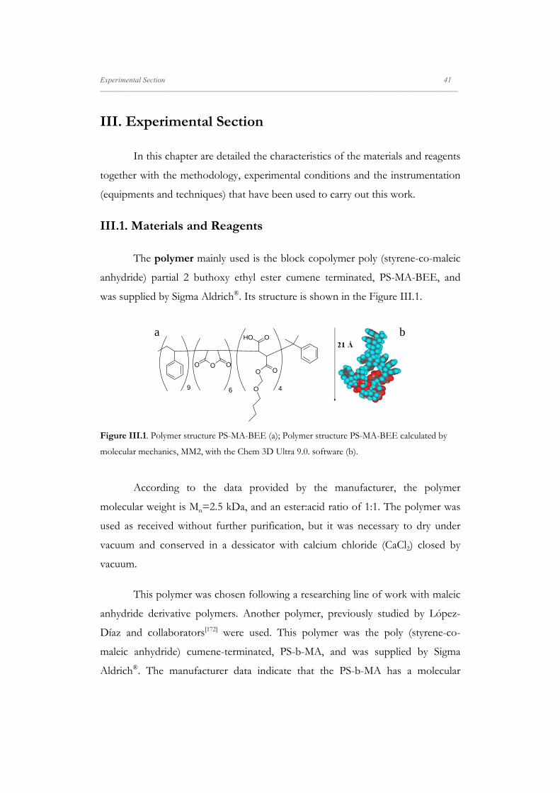
Experimental Section 41 _____________________________________________________________________________________________________________________
III. Experimental Section
In this chapter are detailed the characteristics of the materials and reagents
together with the methodology, experimental conditions and the instrumentation
(equipments and techniques) that have been used to carry out this work.
III.1. Materials and Reagents
The polymer mainly used is the block copolymer poly (styrene-co-maleic
anhydride) partial 2 buthoxy ethyl ester cumene terminated, PS-MA-BEE, and
was supplied by Sigma Aldrich®. Its structure is shown in the Figure III.1.
Figure III.1. Polymer structure PS-MA-BEE (a); Polymer structure PS-MA-BEE calculated by
molecular mechanics, MM2, with the Chem 3D Ultra 9.0. software (b).
According to the data provided by the manufacturer, the polymer
molecular weight is Mn=2.5 kDa, and an ester:acid ratio of 1:1. The polymer was
used as received without further purification, but it was necessary to dry under
vacuum and conserved in a dessicator with calcium chloride (CaCl2) closed by
vacuum.
This polymer was chosen following a researching line of work with maleic
anhydride derivative polymers. Another polymer, previously studied by López-
Díaz and collaborators[172] were used. This polymer was the poly (styrene-co-
maleic anhydride) cumene-terminated, PS-b-MA, and was supplied by Sigma
Aldrich®. The manufacturer data indicate that the PS-b-MA has a molecular
OHO
OO OO
9 6 4O
O
a b
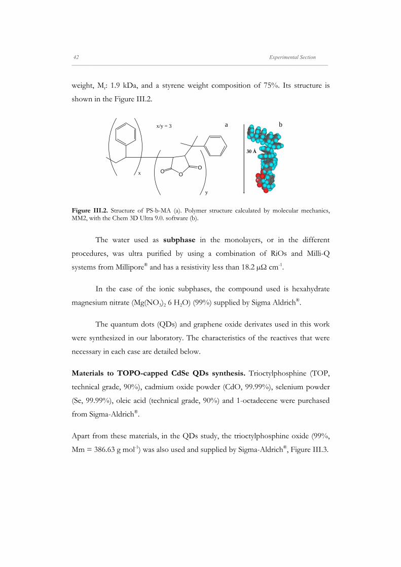
42 Experimental Section _____________________________________________________________________________________________________________________
weight, Mr: 1.9 kDa, and a styrene weight composition of 75%. Its structure is
shown in the Figure III.2.
Figure III.2. Structure of PS-b-MA (a). Polymer structure calculated by molecular mechanics, MM2, with the Chem 3D Ultra 9.0. software (b).
The water used as subphase in the monolayers, or in the different
procedures, was ultra purified by using a combination of RiOs and Milli-Q
systems from Millipore® and has a resistivity less than 18.2 µΩ cm-1.
In the case of the ionic subphases, the compound used is hexahydrate
magnesium nitrate (Mg(NO3)2 6 H2O) (99%) supplied by Sigma Aldrich®.
The quantum dots (QDs) and graphene oxide derivates used in this work
were synthesized in our laboratory. The characteristics of the reactives that were
necessary in each case are detailed below.
Materials to TOPO-capped CdSe QDs synthesis. Trioctylphosphine (TOP,
technical grade, 90%), cadmium oxide powder (CdO, 99.99%), selenium powder
(Se, 99.99%), oleic acid (technical grade, 90%) and 1-octadecene were purchased
from Sigma-Aldrich®.
Apart from these materials, in the QDs study, the trioctylphosphine oxide (99%,
Mm = 386.63 g mol-1) was also used and supplied by Sigma-Aldrich®, Figure III.3.
OO
O
y
x
x/y = 3
30 Å
a b

Experimental Section 43 _____________________________________________________________________________________________________________________
Figure III.3. Molecular Structure of trioctylphosphine oxide molecule, TOPO, and the optimum
conformation calculated within the MM2 approximation.
Materials to graphene oxide derivatives. The batch material (carbon source)
was natural graphite flakes, 99.02 fixed C, from Qingdao super graphite Co., LTD
(Chine). Other materials were: NaNO3 (99%), H2SO4 (98%w), KMnO4 (>99%),
H2O2 (30%w), hydrazine hydrate (80%w) and Vitamin C (ascorbic acid, puriss.)
were purchased from Sigma-Aldrich® and used as received without further
purification.
The zwitterionic surfactant, dodecyl dimethyl ammoniopropane sulfonate
(DDPS, cmc 25.3·10-4 M, Mm = 335.55 g mol-1), Figure III.4, was purified by
recrystallization in isopropanol until obtain constancy in the surface tension value
of a surfactant solution of concentration close to the cmc, critical micelle
concentration, as previously reported.[173, 174]
P
O
1.05nm
a b

44 Experimental Section _____________________________________________________________________________________________________________________
Figure III.4. Zwitterionic surfactant structure DDPS (a); Surfactant structure DDPS calculated by
molecular mechanics, MM2, with the Chem 3D Ultra 9.0. software (b).
For the Langmuir-Blodgett deposition, several substrates were used. The
substrates were generally chosen taking into account the requirements of the
experimental techniques. These substrates are: muscovite, mono and
polycrystalline silicon wafers, quartz discs and copper grids.
Muscovite (mica) quality V-1 was supplied by EMS (USA). The mica
surface was freshly cleaved before use.
Silicon monocrystalline wafers, Si(100), supplied by Siltronix (France), are
single side polished and were used without pretreatment.
Silicon polycrystalline wafer were supplied by Graphene Industries (U.K.).
These As-doped wafers has a dry thermal 280-310 nm silicon oxide (SiO2) layer, a
resistivity of 0.001-0.050 Ω cm-1, a single side polished and gold-alignment laser
marks (spacing 200 µm). This substrate was used in the study of graphene
derivatives. Thus, we use a silicon wafer with thickness of around 300 nm of SiO2
in order to enhance the optical contrast of the graphene flakes under white-light
illumination for Raman measurements.[175] The cleaning procedure [176] for these
wafers was by mild sonication with acetone (PAI quality, Panreac®) (30 s),
methanol (PAI quality, Panreac®) (30 s) and MilliQ water (30 s) and finally dried in
an oven at 90ºC.
N
SO
O
Oa b
17Å

Experimental Section 45 _____________________________________________________________________________________________________________________
Quartz discs (diameter 1 inch; thickness 1/8 inch, polished) were cleaned
by the RCA procedure.[176] Firstly, the discs were cleaned with acetone (PAI
quality, Panreac®), ethanol (PAI quality, Panreac®) and MilliQ water. In a glass
beaker MilliQ water and ammonia (25% vol, Sigma Aldrich®) (5:1 v/v) are mixed
up to 60 mL and heated until 70ºC, and then 10 mL of hydrogen peroxide (30%w,
Panreac®) are added. Then discs are submerged and maintained during 15 min at
70ºC. After, the discs are rinsed with abundant MilliQ water and dried. These
substrates were supplied by TedPella (USA).
Formvar®-carbon coated copper grids were supplied by the Servicio de
Microscopía Electrónica (Universidad de Salamanca). The carbon copper grids
were from TedPella (USA).
III.2. Langmuir Monolayers: Preparation Procedure
Chloroform was used to prepare the spreading solutions of the different
materials (polymer, nanoparticles and graphene derivatives) in order to form the
Langmuir monolayers on the subphase. The solvent is PAI quality, filtered and
supplied by Sigma Aldrich®. The selection of this solvent is due to present good
spreading characteristics on the air-water interface [87] and also is a good solvent
for the different materials.
Cleaning procedure for the different components of the Langmuir trough
is the following. The trough is washed with water and abundantly rinsed with
lukewarm MilliQ water. Next, it is cleaned with acetone (PAI quality, Panreac®) in
order to eliminate the rest of water; chloroform (PAI quality, Panreac®) and again
with acetone to eliminate the rest of chloroform. Finally, the acetone, which
remains, is swept out with abundantly MilliQ water. Also, a Derquim® (Panreac)
cleaning is used once a month.

46 Experimental Section _____________________________________________________________________________________________________________________
Pt-Wilhelmy plate is burned with methanol to eliminate the remains of
material adsorbed. Once a week, it is cleaned by using a 1 M solution of
hydrochloric acid (HCl, Panreac®).
In order to guarantee the correct cleaning of the subphase, the surface
tension is measured at several areas, thus, if it differs of the value for the subphase
at the working temperature, the barriers are compressed (closed) and the interface
is sucked up with a glass Pasteur pipette connected to a water pump (Oakton WP-
15-1 model) until to achieve the right surface tension. When the surface of
subphase was compressed, it is checked that the surface pressure did not exceed
0.3 mN m-1 during the compression, also ensuring the cleaning.
Deposition of materials on the interface is carried out by the addition of
small volumes (10-50 µL) of the prepared solution using a Hamilton microsyringe
(precision ± 1µL), on different zones of the interface. After the addition, the wait
time to ensure the solvent evaporation and the right formation of the monolayer
is 20-30 min.
The experimental conditions for the Langmuir films preparation of the
different materials are detailed below.
For the polymer films the concentrations of the spreading solution in
chloroform were ca. 0.06 mg mL-1 for PS-MA-BEE and 0.70 mg mL-1 for PS-b-
MA and were prepared by weight using an analytical balance precise to ± 0.01 mg.
The polymer monolayer was transferred to solid substrates by compression at a
barriers speed of 5 mm min-1, with the substrate into the trough by vertically
dipping it up at 5 mm min-1.
In the case of QDs and QD/polymer mixed films the concentrations
range for the components in the spreading solutions prepared in chloroform were
from 2·10-7 to 1·10-6 M and 0.060 to 0.0002 mg mL-1 for QDs and PS-MA-BEE,
respectively, depending on the mixture mole ratio. Monolayers were transferred to
Experimental Section 47 _____________________________________________________________________________________________________________________
solid substrates by compression at a barriers speed of 5 mm min-1, with the
substrate into the trough by vertically dipping it up at 5 mm min-1, except for the
copper grids. In the case of copper grids for TEM measurements, the rate of
dipping up was reduced to 2 mm min-1. The subphase temperature was
maintained in all the experiments at 23.0 ± 0.1ºC (296K).
Finally, the GO Langmuir films were prepared by spreading a dispersion
(~0.5 mg mL-1) in MeOH:H2O (5:1 v/v, sonication 30 min) on the air-water
interface. The GO sheets were transferred onto silicon by symmetric barrier
compression (50 mm min-1) with the substrate into the trough by vertically
dipping it up at 2 mm min-1 by LB method. On the other hand, the RGO sheets
were deposited onto the water subphase using a dispersion (~0.1 mg mL-1) in
chloroform. The RGO sheets were transferred from the air-water interface onto
silicon by symmetric barrier compression (50 mm min-1) with the substrate into
the trough by vertically dipping it up at 5 mm min-1. The water subphase
temperature was maintained in all the experiments at 20.0 ± 0.1ºC (293K).
III.3. Experimental Techniques
In this section are briefly described the equipments and techniques
employed in the research together with the work conditions used to carry out the
measurements.
III.3.1. Langmuir Trough
The equipment, which was used to prepare the surface pressure isotherms
and the rheological study of the insoluble monolayers, is a teflon trough (KSV
Instruments LTD Mini model, Finland) controlled by computer. A photograph of
it is showed in the Figure III.5. The main components of the equipment are: the
trough, the movable barriers and the electrobalance.

48 Experimental Section _____________________________________________________________________________________________________________________
Figure III.5. Photograph of the Mini model trough (KSV Instrument LTD).
The trough, built in teflon, with dimensions of 32.4 x 7.5 cm, has an area
of 243 cm2 and contains the subphase, water or an aqueous solution of different
electrolytes. As teflon is a hydrophobic material the subphase adopts the form of
the trough edges and with the water forms a contact angle next to π/2 avoiding the
wetting phenomena. The subphase temperature is maintained with through
jackets at the bottom of the trough by flowing thermostated water from a
thermostat/cryostat Lauda Ecoline RE-106. The temperature near the surface was
controlled/measured with a calibrated sensor from KSV Instrument LTD.
Movable barriers are built with a hydrophilic material called Delrin®
(polyoxymethylene), thus they form a concave curvature with the subphase
avoiding the material loose of the monolayer under the barriers. In order to
ensure that the area changes are produced in the perpendicular plane to the liquid
surface, the barriers are placed on stainless steel pieces and connected to an
electromechanic device that automatically controls their movement, allowing to
programme different kinds of experiments. The speed range for the barriers
movement goes from 1 to 120.5 mm min-1.

Experimental Section 49 _____________________________________________________________________________________________________________________
Equilibrium Measurements
The surface pressure was measured with a Pt-Wilhelmy plate connected to
an electrobalance. The plate is placed at the air-water interface, thus, the surface
pressure is directly determined without correction of the obtained values. The
porous Pt-plate forms a nulling contact angle with the subphase, so the surface
wetting was right. As the plate is hung from an electrobalance, when the plate
makes contact with the interface, an increasing of weight, ΔW, is produced, that is
related to the surface tension following the expression:
Δ
III. 1
Where, p, is the perimeter of the plate (10x19.62 mm), and θ, the contact angle
between the subphase and the plate that comes from:
1 III. 2
In this expression a and h represent the capilar length and the height of the top
part of the meniscus formed over the liquid surface level, respectively.
The electrobalance is able to measure surface pressures of 0.01 mN m-1,
but the data precision in the experimental conditions is not more than 0.1 mN m-
1, due to the influence of external factors as the temperature and mechanical
stability. In order to minimize the mechanical vibrations, the trough is placed on
an anti-vibration table.
The equipment allows to characterize the Langmuir monolayer measuring
different physical properties as surface pressure and potential while the available
area is being modified with a movable barriers mechanical system by symmetric
compression or expansion.
50 Experimental Section _____________________________________________________________________________________________________________________
Dynamic Measurements
In the dynamic studies of insoluble monolayers, the system in equilibrium
is disturbed. An option to perturb the monolayer are the relaxation experiments,
that consist of apply a distortion (deformation) to the system and analyze the
response of this with the study of the relaxation of the tensions that act on the
system by recording the temporal variation of the surface pressure. Depending on
the type of deformation applied, there are two kinds of experiments: sudden-step
method and dynamic oscillation method (sinusoidal deformation).
The sudden-step experiments, i.e., step-compression or step-expansion
are quickly carried out by moving the barriers (120.5 mm min-1) in order to
modify the available area in the monolayer controlled with the software. The time
necessary to make the compression was slightly less than 2 s. The system response
is measured by recording the surface pressure with the time. When the trough
area is modified then the surface concentration is also modified, i.e., during the
compression the system losses the equilibrium and an increase in the surface
pressure is produced. When the compression stops, the relaxation of tensions in
the monolayer begins decreasing the surface pressure until a constant value is
reached, that corresponds to the pressure value of the new equilibrium. A scheme
of the process, for a step-compression, is showed in Figure III.6.

Experimental Section 51 _____________________________________________________________________________________________________________________
Figure III.6. Representative scheme of a step-compression experiment.
In small and independent molecules, i.e., without interaction with the
environment molecules, the response of the surface pressure can be interpreted as
a Debye exponential relaxation [133]:
III. 3
In this equation τ and σ0 represent the relaxation time and the relaxation
amplitude, respectively.
From the values of the area increment (strain), -ΔA/A0, and the relaxation
amplitude, σ0, are determined the dynamic elasticity, ε, and the dilatational
viscosity, , [177] by using the following expressions:
Δ ⁄ III. 4
Δ ⁄ III. 5

52 Experimental Section _____________________________________________________________________________________________________________________
The dynamic elasticity represents the instantaneous elastic response of the
monolayer, while the dilatational viscosity represents the friction losses that are
produced.
The dynamic oscillation experiments consist of the sinusoidal
deformation as a time function of the available area in the monolayer. In order to
carry out oscillatory barrier movements are programmed maintaining the
frequency constant. Thus, by the analysis of the surface pressure response with
different changes of area (strain), it is possible to determine the strain range in
which the system response is linear.
The variation function of the area with the time is expressed by the
following equation:
21 III. 6
Where, U(t) = ΔA/A0. The parameters U0, ω and φu, are respectively the
deformation amplitude (strain), the angular velocity and the phase lag angle with
regard to the equilibrium position of the wave. Figure III.7. shows the
experimental results for a PS-MA-BEE monolayer deposited on an aqueous
subphase.

Experimental Section 53 _____________________________________________________________________________________________________________________
Figure III.7. Graph of a PS-MA-BEE monolayer response due to a sinusoidal area change, U(t)
at 296 K.
The strain promotes the modification of the surface concentration and as
result, a change in the surface pressure that depends on the time according to the
expression:
21 III. 7
Where π0, is the equilibrium surface pressure, σ0, the amplitude of the stress
(system response) and φσ, the phase lag angle with regard to the equilibrium
position of the surface pressure wave.
In this work, several measurements were carried out by the step-
compression method. However, to use this technique, it is necessary to work in
the linear regime, i.e., the range where the amplitude of the stress is proportional
to the strain, according to Hooke's Law. To check the strain range, oscillatory
barrier measurements were carried out in the monolayers.

54 Experimental Section _____________________________________________________________________________________________________________________
III.3.2. Surface Potential: Kelvin Probe
Surface potential is a magnitude that gives information not only about the
structure of the double dielectric layer of the adsorbed molecules at the interface,
but also about the orientation of the molecules at the interface. When an adsorbed
monolayer exists at a fluid interface, a sensible increase of the existent Volta
potential between this surface and a metal electrode placed on a certain distance is
produced. In a Langmuir monolayer the surface potential measures as the
presence of the monolayer affects the potential of the clean subphase, thus the
surface potential is termed as the difference in potential between a monolayer-
covered subphase and a clean subphase.[79]
Δ III. 8
This magnitude is measured with the ionizing probe technique or the
vibrating capacitor technique. The first method, actually in disuse, implies the use
of a fix electrode of polonium or another emitter of particles α, that cause the
ionization of the air gap between the fluid surface and the electrode, making it
sufficiently conductor to determine the impedance between this electrode and one
of reference introduced in the subphase. A method more precise, and that not use
radioactive material, is the method used in this work. It is the noncontact
vibrating electrode (plate) capacitor or Kelvin probe method. It consists of a
metal electrode (plate) located at approximately 2 mm above the aqueous surface
and other as reference submerged in the subphase. If the plate is made to vibrate,
the distance between the plate and the interface changes, and therefore, the
capacity of the formed condenser changes, appearing an alternating current over
to the applied potential. This current is proportional to the surface potential. The
equipment cancels this current by applying an external bias till the potential
difference between the plates is zero. The Kelvin probe used in this work is the
SPOT2 model from KSV Instrument LTD and allows us to obtain values of

Experimental Section 55 _____________________________________________________________________________________________________________________
surface potential with a precision of 20 mV. The surface potential of
monolayers was determined relative to the surface potential of the supporting
electrolyte and of water if no salt was added to the subphase. Each reported value
is an average over five measurements and the standard deviation of these
measurements was considered the experimental error. In Figure III.8. a
photograph of the equipment is showed.
Figure III.8. Photograph of the Kelvin probe SPOT 2 model (KSV Instrument LTD) placed on
the Langmuir trough.
Theoretical models have been developed in the course of the years to
interpret the surface potential measurements and to relate quantitatively the
measured potentials to the group dipole moment of the film-forming molecules.
Such models are based on the Helmholtz model [178], in which the interface
structure is considered as a parallel plate condenser, with plates spaced a distance,
d, equal to the interface thickness, and charged with opposite signs and a surface
density of charge, σ. Therefore, comprising a sheet of uniformly distributed
dipoles, leading to an increase of surface potential described by:
Δ4
III. 9

56 Experimental Section _____________________________________________________________________________________________________________________
Where and 0, are the electric permittivity of the monolayer and the permittivity
of free space, respectively; d, represents the monolayer thickness; and µn, is the
normal component of the dipole moment per adsorbed molecule.
Improvements of the Helmholtz equation have been made in order to
take into account the dipole moment contributions from distinct molecular
groups. Davies and Rideal [179] proposed the decomposition of the dipolar
moment, µn, in three components: µ1, is the contribution from reorientation of
water molecules from the subphase due to the presence of the monolayer; µ2, is
the contribution from head groups; and µ3, arises from the hydrophobic moiety.
Since it is impossible to measure µ1 independently, it is customary to combine
with µ2 as the former anyway depends on the type of the head group. This was the
approach adopted by Vogel and Möbius [180], in which the monolayer is modelled
as a two-layer capacitor. Thus the effective dipole moments are divided into two
contributions, from the air-film interface, µα, and film-water interface, µβ, and the
surface potential can thus be expressed as follows:
Δ
III. 10
When the film is compressed, the surface potential changes due to alteration of
either the head or the tail group orientation.
Demchak and Fort [181], introduced the concept of effective relative
permittivities for different regions which allows to take into account the induced
polarization due to neighbouring molecules, in this way, proposed the three-layer
capacitor, in which the monolayer surface potential is expressed as:
Δ1
III. 11

Experimental Section 57 _____________________________________________________________________________________________________________________
The contribution µ1/ε1 is due to reorientation of water molecules, while
µ2/ε2 and µ3/ε3 correspond to hydrophilic and hydrophobic group regions,
respectively.
In the Figure III.9. is showed a scheme of the three explained models.
Figure III.9. Models to explain the non-ionic monolayer surface potential.
The surface potential has a value close to zero in gaseous monolayers very
expanded. The apparition of a value of surface potential different to zero, at high
areas per molecule of the isotherm, is attributed to impurities in the subphase.[182]
When the density of adsorbed molecules increasing, even at surface pressure
values close to zero, the potential begins to increase. The area at which the
potential begins to significantly increase is denoted as critical area and is usually
located around two times the area at the beginning of the surface pressure
increase. The existence of the critical area has been related to the formation of
structures by hydrogen-bonding between the water molecules and polar groups of
Hydrophobic regionµ3, ε3
µ1,ε1
Hydrophilic region
Aqueous Subphase
µ2, ε2
Hydrophobic region
Hydrated polar group regionµa
µw
- - - - - - -
+ + + + + + +
µn, εHelmholtz Model
Vogel and MöbiusModel
Demchak and Fort Model

58 Experimental Section _____________________________________________________________________________________________________________________
the molecules that forms the monolayer. The observation of the intermolecular
interaction is consistent with the results obtained by Brewster angle microscopy
(BAM) or fluorescence.
In ionic monolayers is formed a double-layer electric below the interface
that contributes to the surface potential in a quantity, Ψ0, that is included in the
Helmholtz equation to calculate the monolayer potential. The value of Ψ0 can be
obtained solving the Gouy-Chapman model for the electric double-layer.[183]
Δ
Ψ . 12
III.3.3. Brewster Angle Microscopy (BAM)
Brewster Angle Microscopy was independently introduced by two
groups[184, 185] to the characterization of the molecular monolayers at the air-water
interface, due to probe information about the two-dimensional organization of
adsorbed material, including size and shape of co-existence phase domains and
also the heterogeneity that appears in Langmuir films. The main advantage of this
technique is that it does not contact with the monolayer, therefore it does not
modify the formed structures, not contaminate, as it can occur in the case of the
epifluorescence microscopy.[186]
This technique is based on the behaviour that the polarized light presents
when is reflected on a dielectric thin surface. When this occurs, the incident light
beam on the surface is transformed in a partial polarized light beam. It means that
the reflected electric vector vibrates in the parallel plane to the material surface.
The intensity of the reflected light depends on the incident angle. For a polarized
light beam parallel to the incident plane exists an angle in which there is not
reflection. This angle is called Brewster angle, and for the case of the air-water
interface has a value of 53.1º.[79]
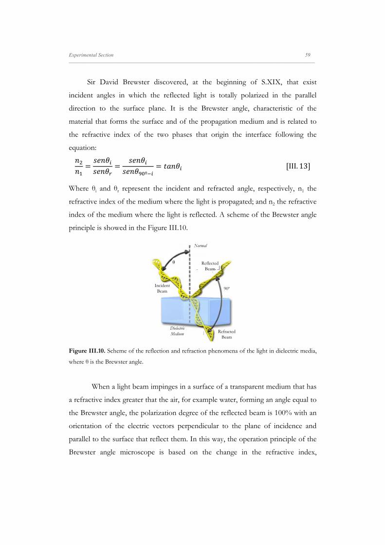
Experimental Section 59 _____________________________________________________________________________________________________________________
Sir David Brewster discovered, at the beginning of S.XIX, that exist
incident angles in which the reflected light is totally polarized in the parallel
direction to the surface plane. It is the Brewster angle, characteristic of the
material that forms the surface and of the propagation medium and is related to
the refractive index of the two phases that origin the interface following the
equation:
ºIII. 13
Where θi and θr represent the incident and refracted angle, respectively, n1 the
refractive index of the medium where the light is propagated; and n2 the refractive
index of the medium where the light is reflected. A scheme of the Brewster angle
principle is showed in the Figure III.10.
Figure III.10. Scheme of the reflection and refraction phenomena of the light in dielectric media,
where θ is the Brewster angle.
When a light beam impinges in a surface of a transparent medium that has
a refractive index greater that the air, for example water, forming an angle equal to
the Brewster angle, the polarization degree of the reflected beam is 100% with an
orientation of the electric vectors perpendicular to the plane of incidence and
parallel to the surface that reflect them. In this way, the operation principle of the
Brewster angle microscope is based on the change in the refractive index,
ReflectedBeam
IncidentBeam
RefractedBeam
90º
Normal
DielectricMedium

60 Experimental Section _____________________________________________________________________________________________________________________
therefore, in the change in the Brewster angle originated when a material is
deposited at the air-water interface in order to form the monolayer and that
produces the reflection of the light. A scheme of this phenomenon is showed in
Figure III.11.
Figure III.11. Scheme of the reflection phenomenon due to the presence of a monolayer at the
air-water interface, where the incident angle θB is the Brewster angle.
The Brewster angle microscopy used in this work is from KSV Instrument
LTD (Finland), Optrel BAM 3000 model. In general, a microscopy of these
characteristics has the following components: Goniometer, Light source and
Analysis module. A photograph of BAM is shown in Figure III.12.
Goniometer
Goniometer (1) is composed by two movable pieces that allow modifying
the height with regard to the interface and the angle that forms these pieces. In
each piece there are placed the light source and the analysis module.
Light Source
Light source is a He-Ne laser (2) that emits light in a wavelength of 632.8
nm with a power of 10 mW. It is joined to a polarizer (3) that polarizes the light
emitted by the laser.
Monolayer
Air
ReflectionNo reflection
θB
Aqueous Subphase
θB

Experimental Section 61 _____________________________________________________________________________________________________________________
Figure III.12. Brewster Angle Microscopy Optrel BAM 3000 (KSV Instrument LTD).
Analysis Module
Analysis module consists of objective, polarizer and camera. The optical
objective (4), with a capacity of 5 magnifications (5X), is from Mitutoyo (USA).
Joined to this, there is a polarizer (5), which fit the direction of polarization that
comes from the surface. Finally, the light arrives to a digital high resolution
monochromatic camera (6) from EHD (Kam Pro-02 model) that has a resolution
of 768 X 494 pixels.
This technique allows us to study of the interface morphology due to
taking into account that as the light in the Brewster angle is polarized in the
direction of the surface, i.e., the air-water interface, if a polarizer is perpendicularly
placed on the reflected beam, the image collected by the camera will be null,
because no light arrives. However, when a material is deposited to form an
insoluble monolayer, the refractive index changes and therefore the Brewster

62 Experimental Section _____________________________________________________________________________________________________________________
angle changes, arriving light to the camera and allowing to see an image. If the
monolayer has phases with different refractive index, the images show bright and
dark domains (areas) depending on the difference of the phase angle with regard
to the Brewster angle of the interface.
BAM images are digitalized and filtered in order to reduce diffraction
fringes caused by the coherent nature of the laser beam and finally processed to
improve quality. In this way, the images provided by BAM are zones of different
tonality that are related to either different phases of the monolayer.[79]
III.3.4. Langmuir-Blodgett Trough
The equipment for the deposition of LB films was a teflon trough
(KSV2000 Standard model, Finland) controlled by computer (Figure III.13). This
trough is similar to the Langmuir trough before explained. In this case the trough
has an area of 780 cm2 (dimensions 52 x 15 cm).
Figure III.13. Langmuir-Blodgett Standard trough (KSV Instruments). The inset shows the
dipping arm which holds the substrates for the LB deposition.
The transfer of the Langmuir monolayers from the air-water interface to
solid substrates is carried out by using a dipper (dipping arm which holds the
substrate) connected to the trough and the computer interface. The dipper is

Experimental Section 63 _____________________________________________________________________________________________________________________
controlled by computer and moves perpendicular to the interface. For the
transfer is important the control and optimization of several parameters
depending on the type of monolayer and substrate: the transfer ratio, the
compression rate of the monolayer and the dipping speed (immersion or
emersion) during the deposition. Other factors that affects to the process are:
surface pressure, type of molecules that forms the monolayer and composition,
temperature and pH of the subphase. The LB film deposition was carried out by
dipping up, i.e., firstly the substrate is submerged, then the monolayer is formed
and finally, the monolayer is transferred by move up the substrate. In general, for
dipping starting from below the air-liquid interface, the substrate is hydrophilic,
and for dipping starting above the air-liquid interface the substrate is
hydrophobic. Multilayers can be achieved by successive dipping through
alternating monolayers.[86, 187] During the transfer, surface pressure is maintained
constant by symmetric compression of the barriers. The used substrates were
quartz, muscovite (mica), silicon and copper grids (for TEM).
III.3.5. Atomic Force Microscopy (AFM)
The AFM technique was used to characterize the morphology and
thickness of the different studied Langmuir-Blodgett films deposited onto several
substrates. The measurements was carried out under laboratory conditions at
constant repulsive force mode by using an AFM (Nanotec Cervantes-Dulcinea,
Spain) with a rectangular microfabricated silicon nitride (Si3N4) cantilever
(Olympus OMCL-RC800PSA) with a length of 100 µm, with a silicon pyramidal
tip and a spring constant of 0.73 mN m-1. The scanning frequencies rate were
usually in the range 0.5-1.2 Hz per line. The equipment is located in an
antivibration table, and in several times, it was necessary to minimize the
environment acoustic and electronic noise. The acquisition and analysis were
carried out with the WSxM 5.0 software free supplied by Nanotec.[188] The

64 Experimental Section _____________________________________________________________________________________________________________________
measurements were done in the Ultrashort Ultraintense Pulsed Lasers Centre
(CLPU) of the Universidad de Salamanca.
Although the resolution depends on the type of sample, generally, the
technique has a resolution around 0.01 nm for heights (z) and a lateral resolution
(x, y) of 0.7-5nm for soft materials. The running of this technique is based on the
interaction/repulsion forces between the tip, which scans the surface of the
sample keeping up to a distance, and the material of the sample that is studied.
The tip is anchored to a cantilever, because of it, according to the interactions
between the tip and the surface of the sample, the distance between both is
modified. This distance is optically controlled by the system, during the scan of
the sample, by a laser beam focus on the back of the cantilever for monitoring its
shift (deflection), Figure III.14. The reflected beam is collected by a photodiode
that multiplies the cantilever shift (deflection), improving the sensibility of the
equipment, and through a feedback circuit controls the distance tip-sample that
the software converts into the topographic map of the surface sample. During the
scan of the sample surface, the movement (3D position) of the tip is controlled by
a scanner built onto a piezoelectric system.
Figure III.14. Schematic picture of the main components of the AFM.
Photodetector
Laser Beam
Cantilever

Experimental Section 65 _____________________________________________________________________________________________________________________
The main interaction force between the tip and the sample is the Van der Waals
force, which depends on their distance (Figure III.15). In the contact regime, the
probe (tip-cantilever) is held less than a few angstroms from the sample surface,
and the interatomic force between the probe and the sample is repulsive. In the
non-contact regime, the probe is held on the order of tens to hundreds of
angstroms from the sample surface, and the interatomic force between the
cantilever and sample is attractive (largely a result of the long-range Van der Waals
interactions).
Figure III.15. Potential energy (V(z)) vs distance (z) diagram between a probe and a sample.
The usual operation modes for this equipment are:
Contact Mode. In this case, the tip slightly contacts with the surface of the
sample. It is possible to work by two ways, fixing the distance between
tip-surface or establishing the force applied by the tip onto the sample,
due to the deflection of the cantilever is proportional to the force acting
on the tip, according to a Hooke's Law, where k is the spring constant of
the cantilever. By this mode, it is possible to manipulate or damage the
sample and contaminate the tip.
Interaction Force
Tip atoms
Surface atoms
V(z)
zNon‐contact modeContact mode
Repulsive Region
Attractive Region
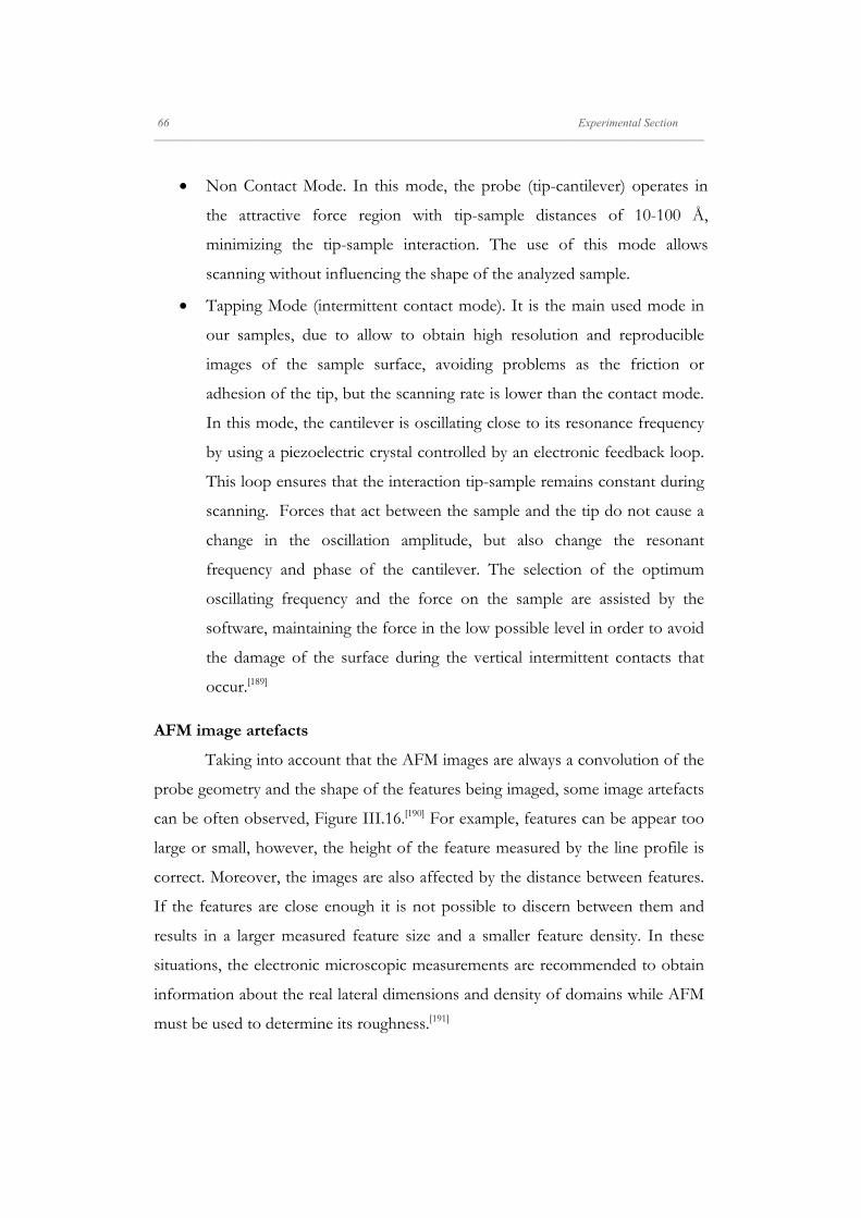
66 Experimental Section _____________________________________________________________________________________________________________________
Non Contact Mode. In this mode, the probe (tip-cantilever) operates in
the attractive force region with tip-sample distances of 10-100 Å,
minimizing the tip-sample interaction. The use of this mode allows
scanning without influencing the shape of the analyzed sample.
Tapping Mode (intermittent contact mode). It is the main used mode in
our samples, due to allow to obtain high resolution and reproducible
images of the sample surface, avoiding problems as the friction or
adhesion of the tip, but the scanning rate is lower than the contact mode.
In this mode, the cantilever is oscillating close to its resonance frequency
by using a piezoelectric crystal controlled by an electronic feedback loop.
This loop ensures that the interaction tip-sample remains constant during
scanning. Forces that act between the sample and the tip do not cause a
change in the oscillation amplitude, but also change the resonant
frequency and phase of the cantilever. The selection of the optimum
oscillating frequency and the force on the sample are assisted by the
software, maintaining the force in the low possible level in order to avoid
the damage of the surface during the vertical intermittent contacts that
occur.[189]
AFM image artefacts
Taking into account that the AFM images are always a convolution of the
probe geometry and the shape of the features being imaged, some image artefacts
can be often observed, Figure III.16.[190] For example, features can be appear too
large or small, however, the height of the feature measured by the line profile is
correct. Moreover, the images are also affected by the distance between features.
If the features are close enough it is not possible to discern between them and
results in a larger measured feature size and a smaller feature density. In these
situations, the electronic microscopic measurements are recommended to obtain
information about the real lateral dimensions and density of domains while AFM
must be used to determine its roughness.[191]
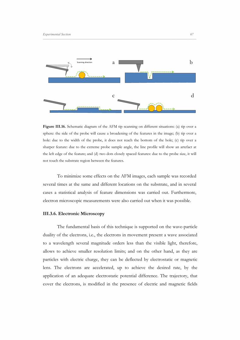
Experimental Section 67 _____________________________________________________________________________________________________________________
Figure III.16. Schematic diagram of the AFM tip scanning on different situations: (a) tip over a
sphere: the side of the probe will cause a broadening of the features in the image; (b) tip over a
hole: due to the width of the probe, it does not reach the bottom of the hole; (c) tip over a
sharper feature: due to the extreme probe sample angle, the line profile will show an artefact at
the left edge of the feature; and (d) two dots closely spaced features: due to the probe size, it will
not touch the substrate region between the features.
To minimize some effects on the AFM images, each sample was recorded
several times at the same and different locations on the substrate, and in several
cases a statistical analysis of feature dimensions was carried out. Furthermore,
electron microscopic measurements were also carried out when it was possible.
III.3.6. Electronic Microscopy
The fundamental basis of this technique is supported on the wave-particle
duality of the electrons, i.e., the electrons in movement present a wave associated
to a wavelength several magnitude orders less than the visible light, therefore,
allows to achieve smaller resolution limits; and on the other hand, as they are
particles with electric charge, they can be deflected by electrostatic or magnetic
lens. The electrons are accelerated, up to achieve the desired rate, by the
application of an adequate electrostatic potential difference. The trajectory, that
cover the electrons, is modified in the presence of electric and magnetic fields
Scanning direction a b
c d

68 Experimental Section _____________________________________________________________________________________________________________________
conveniently placed in order to achieve that the divergent electron beam from the
objective can focus on a point forming an enlarged image of the sample. In this
way, the electrostatic lens are used in the illumination system of the microscopy to
extract and accelerate the electrons; and the magnetic lens to control the current
density of the beam, its displacement and projection.
When the electron beam comes into contact with a sample, a series of
interactions, which are responsible for the observed images contrast, are produced
and give rise to different secondary radiations that can be used to obtain
complementary information. This allows to combine observation and analysis
giving rise to different types of microscopes. If the sample is thin enough, a great
part of the incident electrons will achieve to pass through it, without changes in
their trajectory and energy, producing the transmitted beam, Figure III.17. Part of
the incident electrons can be scattered forward or backward, giving rise to the
scattered beam and the backscattered beam, respectively, with energies that vary
from the initial to several eV.[192]
Figure III.17. Scheme of the resulting interaction of the electron beam with the sample.
In the Transmission Electron Microscopy (TEM), a sample thin enough
(≤ 200 nm), in order to be transparent for the electrons, is irradiated with a
parallel electron beam of uniform current density that goes through the sample
forming an image of the crossed section. In this work, the samples were deposited
onto Formvar®-carbon coated copper grids by the Langmuir-Blodgett technique.
Incident Beam
Scattered Beam
Transmitted Beam
Backscattered Beam

Experimental Section 69 _____________________________________________________________________________________________________________________
Mainly, it was used to study the size and distribution of the nanoparticles in the
LB films. The TEM images were acquired with the following equipments: TEM
(ZEISS EM 902, Germany) at a accelerating voltage of 80kV, that belongs to the
Servicio de Microscopía of the Universidad de Salamanca; and a TEM JEOL JEM
4000 EX (100kV) of the Centro de Microscopía Electrónica Luis Brú
(Universidad Complutense de Madrid).
In the Scanning Electron Microscopy (SEM), the electrons are focused on
the surface of a thick sample, opaque to the electrons. The incident electron beam
scans the surface of the sample, and as a result of the interaction with the sample,
a secondary electron emission is produced: the surface reflects and/or
backscatters electrons, that give rise to a signal. This signal is driven to a cathode
ray tube. The emission intensity depends on the incident angle of the electron
beam onto the material surface and therefore, on the sample topography. In this
tube, the signal scans the display synchronized with the electron beam movement
over the sample, forming an image of the surface.[192]
This technique, and concretely, a Field Emission Scanning Electron
Microscopy (FE-SEM) (NovaTM NanoSEM 230, FEI, USA) has allowed the
characterization of the oxidized and reduced graphene flakes deposited onto
polycrystalline silicon, with a 300 nm SiO2 layer, by Langmuir-Blodgett. The
access to this equipment was possible thanks to the collaboration with the Dpto.
Electrónica of the University of Barcelona (Spain). FE-SEM images were acquired
using the high resolution detector in high vacuum (HV) mode, usually applying an
accelerating voltage of 10 kV. The instrument can be operated in two types of
image modes: secondary electron image (SEI) and backscattered electron image
(BEI).

70 Experimental Section _____________________________________________________________________________________________________________________
III.3.7. Ellipsometry
It is a sensitive optical technique for determining properties of surfaces
and thin films, based on the use of elliptically polarized light generated by the
interaction between the linearly polarized light and a surface. The shape and
orientation of the ellipse depend on the angle of incidence, the direction of the
polarization of the incident light, and the reflection properties of the surface. In
this way, it is possible to measure the polarization of the reflected light with a
quarter-wave plate (QWP) followed by an analyzer; the orientations of the
quarter-wave plate and the analyzer are varied until no light passes though the
analyzer. From these orientations and the direction of polarization of the incident
light, it is possible to calculate the relative phase change, Δ, and the relative
amplitude change, Ψ, introduced by reflection from the surface.
An ellipsometer measures the changes in the polarization state of light
when it is reflected from a sample, thus, when the thickness of the sample varies,
change the reflection properties of the light. Measuring these changes in the
reflection properties can allow to deduce the actual change in the film thickness.
As this technique is based on the reflection, some general basics of this
phenomenon are indicated. In the reflection, the plane of incidence contains the
beam light before and after the reflection, and it is perpendicular to the surface.
As the used radiation is plane-polarized, there are two kinds of polarizations:
polarization p, when it is polarized in the plane of incidence and s, when the
polarization is perpendicular to the plane of incidence.

Experimental Section 71 _____________________________________________________________________________________________________________________
Figure III.18. Reflection and transmission of the light in an interface.
For the reflection of radiation in an interface that divides two media,
Figure III.18, where part of the light is reflected and other part transmitted, it is
defined the Fresnel's reflection coefficient, r, as the ratio between the amplitude
of the waves reflected and incidental in the interface. For the two polarization
states, p or s, of the incident light, the Fresnel's coefficients are defined as:
III. 14
Where the superscripts represent the polarization state of the waves (p or s), the
subscripts 1 and 2 the media that divide the interface, and n is the complex index
of refraction. The reflectance, , is defined as the ratio between the incident and
reflected intensities, and is related to r by the expression:
| | | | III. 15
In the analyzed samples, there are multiple interfaces (several layers or media),
because of it, the total reflection is the sum of the reflection in the outer surface,
with all the components of the reflection in each intermediate interface where the
light is transmitted, Figure III.19.
n2
n1
ф1
ф2

72 Experimental Section _____________________________________________________________________________________________________________________
Figure III.19. Reflection and transmission with multiple interfaces.
For these cases, the Azzam's and Heavens' expressions are used. They deduced
the relation between the amplitude of the resultant wave with regard to the
incident wave, i.e., the total reflection coefficients, R.[193, 194]
1
1III. 16
In this expression the subscript ij (i = 1, 2, 3 y j = i+1) is referred to the reflection
coefficient between the media i and j. β is the phase thickness of the film:
2 . 17
where hop is the film's thickness. When hop → 0, the total reflection coefficient is
equal to the Fresnel's coefficient.
As was previously exposed, between the incident and reflected radiation
over the sample, there is a difference or change of phase between the parallel and
perpendicular components, δ. The difference in the phase, between the incident
beam (1) and the reflected beam (2) defines the first ellipsometric angle, Δ, that
varies between 0 and 360º.
ф1
n1
n2
ф2
n3ф3

Experimental Section 73 _____________________________________________________________________________________________________________________
Δ III. 18
Also the amplitude of the light components is modified, and is related to the psi
angle, Ψ, that can vary between 0 and 90º.
tanΨRR
III. 19
These two angles are experimentally determined in the ellipsometric
measurements, and are related to the total reflection coefficients, p, following the
fundamental equation of the ellipsometry.[195]
Ψ III. 20
Equipment and Data Analysis
The measurements were carried out in the CAI of Spectroscopy of the
Universidad Complutense de Madrid, with a nulling ellipsometer EP3 model
(Nanofilm, Germany). Radiation source of the ellipsometer is a Nd-YAG laser
with a wavelength of 532 nm (green) and maximum power of 50 mW, but in
the experiments a power of ~2% was used. The ellipsometric measurements
were carried out by varying the incident angle in the range 50º to 86º and also
the ellipsometer was used as a Brewster angle microscopy to observe the surface
of the sample and choose several points for measurement. The laser beam was
focused on the LB films on silicon substrates positioned on the goniometer
plate.

74 Experimental Section _____________________________________________________________________________________________________________________
Figure III.20. A schematic diagram of a nulling ellipsometer with the quarter-wave plate placed
before the light is reflected from the sample. P: the polarizing prism; QWP: the quarter-wave plate
compensator; S: the sample under study; A: the analyzer prism; D: the light detector.
The main optical elements of the ellipsometer are: the polarizer (P), the
analyzer (A), the quarter-wave plate (QWP) and the detector (D), Figure III.20.
The polarizer and analyzer are used to convert the non polarized light in
polarized light, and to determinate the polarization state of a beam, respectively.
The quarter-wave plate allows to elliptically polarize the components of the wave
that goes out from the polarizer. The ellipticity produced by the plate
compensates the ellipticity produced by the reflection in the surface, thus the
light that arrives into the analyzer was linearly polarized. As detector a CCD
camera is used.
For the data analysis [194] a specific model of interface (two layers) is
proposed. It is characterized by the thickness and refractive index of each layer,
in which the ellipsometric angles, Δ and Ψ, obtained from the experimental
measurements, are fitted. The precision on these ellipsometric angles is ca.
0.0006. The computational analysis of the data is carried out with a numerical
minimization routine such as a Simplex method [196, 197] by fitting the ellipticity
from the Fresnel's equations following the formalism set out by Drude [198]. The
iterative program, developed in Excel® by the Solver® tool, solves these equations
Laser Source
P
QWP
A
D
S

Experimental Section 75 _____________________________________________________________________________________________________________________
by minimizing the differences between the values of the ellipsometric
experimental and calculated angles, extracting the values that better fit for the
thickness and the refractive index. In the two layer model proposed, the first
layer corresponds to the substrate material, silicon with a native oxide layer of ~2
nm, and a refractive index, n = 4.1264 - 0.2300i; the second layer is the LB film
deposited onto the substrate. The thickness of the first layer was determined by
using a clean silicon wafer.
III.3.8. Micro-Raman Spectroscopy
The Raman spectroscopy was used to characterize the graphene oxide and
graphene reduced oxide flakes deposited by the Langmuir-Blodgett technique
onto polycrystalline silicon with a silicon oxide (SiO2) layer of 300 nm that allows
their display by optical microscopy.[175] These measurements were done in the
Departamento de Física Alessandro Volta of the University of Pavia (Italy). The
Raman dispersion measurements were carried out at room temperature with a
micro-Raman spectrometer (Horiba Jobin-Yvon LabRAM HR, U.S.A.) with a
100x objective (confocal microscopy) and a laser focus of 1µm2, Figure III.21.
The spectral resolution of the instrument is approximately 2 cm-1, the spatial
resolution is 0.5 m and the laser excitation wavelength is 632.81 nm. The
equipment has a notch filter before the CCD detector to cut the laser beam.
Before the measurements, an accurate calibration was carried out by checking the
Rayleigh band and Si band at 0 and 520.7 cm-1, respectively. The sample area was
scanned with a spatial resolution of approximately 0.5 µm. The acquisition time
was around a few minutes at each point, while the laser excitation power was kept
below 1 mW to avoid heating and preserve the samples.[199]

76 Experimental Section _____________________________________________________________________________________________________________________
Figure III.21. Photograph of the micro-Raman LabRAM HR model (Horiba Jobin Yvon).
Raman spectroscopy is based on inelastic scattering of monochromatic
light, like from a laser source. Inelastic scattering means that the frequency of
photons in monochromatic changes upon interaction with a sample, the photons
of the laser light are absorbed by the sample and then reemitted. Frequency of the
reemitted photons is shifted up or down in comparison with original
monochromatic frequency, which is called the Raman effect. This shift provides
information about vibrational, rotational and other low frequency transitions in
molecules.
In the case of derivative graphite thin films, the Raman spectrum show
characteristic peaks or bands highlighting the electronic structure of graphite
(graphene, if the film is only a honeycomb carbon layer), mainly dominated by the
sp2 nature of the C-C covalent bonds that form the ring-structure, where the
excitation resonates with π states. Mainly, the study is centred on the D, G and
2D bands. The G band, 1580 cm-1, is due to the bond stretching of all pairs of
sp2 atoms in both rings (C(sp2)-C(sp2)), while the D band, 1350 cm-1, is due to

Experimental Section 77 _____________________________________________________________________________________________________________________
the breathing modes of sp2 atoms in rings. The shift of the G band and the ratio
between the D and G bands intensity indicate the disorder degree in the sp2
structure of the sample. In this way, the average G band position moves from
1581 cm-1 to 1600 cm-1 within an ordered graphite layer, which corresponds to the
reduction of the in-plane correlation length (La). The D band appears and
increases in relative intensity following the Tuinstra & Koening relation, ID/IG ∝
La-1, that indicates the degree of defects and disorder in general of the sample is
proportional to the number of aromatic rings, i.e., the structural quality of the
sample. In fact, this D band appears in the borders of defect-free graphene. The
G band full width at half maximum (FWHM) is a measure of disorder too and
increases continuously as the disorder increases.[200]
On the other hand, the existence of a sufficient concentration of defects in
the aromatic ring network, produces the appearance of a D' band, located at
1620 cm-1, which can partially merge with the G band. The defects would cause
the phonon confinement allowing the Raman activation of the band. Between
these defects could found isolated double bonds C=C that resonant in higher
frequencies than the G band. Likewise, the presence of functional groups as
carbonyl, epoxy or hydroxyl groups, come from a residual oxidation, or amides,
resulting in an increase of the D and G band width.[201]
The 2D band, 2700 cm-1, is correlated to the second order (overtone) of
the D band, and allows to know the number of layers of the sample up to a limit
of five, above it, it is not possible to discern with the bulk graphite 2D band. For
example, if the sample is a bilayer graphene, due to the interaction between the
graphite layers, the π and π* bands splits in four components, with a different gap
for electrons and holes (phonons), giving rise to four possible optical transitions.
This is observed in the appearance of a 2D band which deconvolutes in four
components.[202]
78 Experimental Section _____________________________________________________________________________________________________________________
III.3.9. UV-vis Spectrophotometry
The UV-vis spectrophotometry was used to characterize the nanoparticles
and to analyze the reduction degree of the reduced graphene oxide dispersions.
The equipment was a spectrophotometer Shimadzu UV-2401PC and the spectra
were acquired in the wavelength range from 700 to 200 nm. As it is a usual
technique, a brief description of the fundamental theory is explained. In this
technique, the monochromatic light goes through the sample and it is compared,
the intensity of the transmitted light with the incident light intensity, i.e., the
radiation absorption or transmission of the sample in the UV-vis region
(spectrum).
The absorption of light by a molecule in this region produces the
migration of electrons to high energy orbitals. The absorbance is important
because it is related to the concentration of the specie absorbs light, at a
wavelength, in the sample by the Lambert-Beer's Law.[203] In the special case of
the quantum dots, the quantum confinement plays a key role for the
determination of the size-dependent properties of nanoparticles. In fact, the
transmission and emission colours depend on the nanoparticles size and are a
result of the size-dependent band gaps. Also, the extinction coefficient of the first
excitonic absorption peak depends on the nanoparticle size. This extinction
coefficient is independent of ligand nature, solvent refractive index, fluorescence
quantum yield and the synthesis method, therefore, allows to determinate the
nanoparticle concentration in a solution from its absorbance. Moreover, the
absorption spectrum allows us to know the nanoparticles size by empiric
expressions[204] which relate the nanoparticle diameter and the extinction
coefficient to the first absorption peak position (wavelength).

Experimental Section 79 _____________________________________________________________________________________________________________________
III.3.10. Fourier Transform Infrared Spectroscopy (FTIR)
The FTIR spectroscopy was used, in collaboration with the Departamento
de Química Inorgánica (Universidad de Salamanca), to characterize solid samples
prepared as pellets. In order to prepare the pellets, we grind a small quantity of
sample with KBr, that acts as inert matrix (ratio 1:200). This powder mixture is
them pressed, 8 ton cm-2, in a mechanical press to form a translucent pellet
through which the beam of the spectrometer can pass. The equipment is an
Fourier Transform Infrared (FTIR) spectrometer 1600 (Perkin-Elmer, USA)
controlled by a data unit model 3700. The spectrum was acquired in the frequency
range from 4000 to 400 cm-1. Due to it is a usual technique, a brief description
about the theorical fundament of the technique is exposed. In this technique, the
light is passed through the sample. Some of the light is absorbed by the sample
and some of it is passed through (transmitted). When it is compared the intensity
of the transmitted light with the incident light, i.e., it is analyzed the absorption or
transmission (T) of the sample radiation in the infrared region. The resulting
spectrum represents the molecular absorption and transmission, creating a
molecular "fingerprint" of the sample (intensity vs frequency).
The absorption comes from excitation by bond deformation of tension or
flexion. The tension excitation involves changes in the vibrational frequency of
the atoms bonded throughout the axis bond, while the flexion deformation
involves movements of the atoms outside of the axis bond. Within the possible
deformations in a molecule, only are active to the IR that in which the excitation
exists a change in the bond dipolar moment with respect to the ground state.
Besides, the infrared region contains significant absorption bands, not only due to
fundamental modes of tension and flexion, but also overtones, combination
bands, couplings and Fermi's resonant bands. This technique is used as a
qualitative analysis tool, because of the wavenumber position of the absorption
bands is characteristic of each functional group found in a molecule. Moreover,
80 Experimental Section _____________________________________________________________________________________________________________________
the bands can shift slightly its position due to changes in the molecular
environment.
In the FTIR spectroscopy a key in the equipment is the interferometer, in
which, an incident beam of light strikes a tilted semitransparent surface
(beamsplitter) and divides the source radiation into a reflected and transmitted
wave, generating a retard between the two generated waves. In this way, as the
sample is placed between the outlet of the interferometer and the detector, the
obtained spectrum, called interferogram, is the subtraction between the source
spectrum and the spectrum of the sample, which subsequently is divided by the
reference interferogram in order to obtain the infrared transmission spectrum.
The main advantage of this system is that offers a better relation signal/noise for
a given resolution.[203, 205]
III.3.11. X-Ray Photoelectron Spectroscopy (XPS)
The X-ray photoelectron spectroscopy was used to characterize the
different graphitic materials obtained by oxidation and later reduction of natural
graphite flakes. Powder samples were prepared by filtration of the different
dispersions. Measurements were carried out in the Instituto de Catálisis y
Petroleoquímica (CSIC, Madrid). Samples were analyzed with a VG Escalab 200
R spectrometer (Fisons Instruments, USA) equipped with an excitation source of
MgKα (hν = 1253.6 eV) radiation and a hemispherical electron analyzer, Figure
III.22. The working conditions for the high resolution spectra acquisition were 20
eV analyzer pass energy, and the residual pressure in the analysis chamber was
maintained under 2·10-7 Pa.[206]
Based on the photoelectric effect, this technique consists of the excitation
of a surface with X-Ray photons, which pull out electrons of the atoms of the
studied sample. The measurement of the binding energy of the extracted electrons
of the atom inner (core) levels (localized in the superficial region of a few atomic

Experimental Section 81 _____________________________________________________________________________________________________________________
layers) and of the photoemission peak intensity allows to carry out an elemental
chemical analysis of the surface (identify atoms and their relative concentration)
and to establish the oxidation and coordination state (chemical shift). Also, it is
possible to carry out measurements by varying the incident angle, obtaining
information at different depths from the surface. This technique has a relative
high detection limit.
Figure III.22. A XPS spectrometer schematic diagram.
The interaction of X-ray photons with the atoms of a surface produce
the emission of photoelectrons belonging to the inner levels of the atom, thus
the holes formed are filled with electrons of upper energetic levels producing
fluorescence X-rays emission and Auger emission processes. The kinetic energy
(Ek) of the emitted photoelectron is related to the binding energy (EB, difference
between the energy of the initial and final state, respectively) corresponding to
the electronic level from which it was emitted, and with the incident photon
energy (hν) by the equation III.20, where is the material work-function.
RetardedVoltage
Detector
HemisphericalAnalyzer (e‐)
sample
Vacuum Chamber
Preamplifier
ElectronMultiplier Feed
Negative Feed Postive Feed
Control Mode
Spectrometer Unit Control
Integrationtimer
Discriminator
X‐ray Source
‐1/2 ΔV +1/2 ΔV

82 Experimental Section _____________________________________________________________________________________________________________________
III. 20
From the expression is deduced that the measurement of the photoelectron
kinetic energy allows to determine its binding energy, characteristic of each
chemical element. This allows to identify elements by the fingerprint procedure.
Also, due to the binding energy is, in some ways, a measurement of the intensity
of the interaction between the electron and the nuclear charge, it is possible to
state that it follows the energy of the electronic levels and that increases with the
atomic number.
The binding energy for an atom is affected by changes in the oxidation
state, the ligands electronegativity, the type and number of atom bonds in a
compound, that influence on the charge state of the atom before the ionization
with a X-ray photon. These factors known as initial state effects, produce a shift
of the atomic peak in the photoemission spectrum called chemical shift.
Moreover, the possibility of measurement of chemical shifts is one of the most
important advantages of this technique.
A XPS spectrum is the representation of the number of registered
electrons by the detector as a function of the kinetic or binding energy of the
emitted photoelectron. It contains information about the absorption and
ionization (initial state), the atom response and production of a photoelectron
(final state) and the transport and leak of the electron (intrinsic and extrinsic
energy losses).
Qualitative analysis by XPS is possible for the Z>2 elements (H and He
have not inner electronic levels) with a sensibility around 0.5% and an analytical
minimum depth of one or two atomic layers. In the usual procedure of the XPS
analysis of a sample firstly it is registered a general spectrum of the sample from 0
to 1000 eV binding energy for the identification of the elements presented in the
Experimental Section 83 _____________________________________________________________________________________________________________________
excited sample. Then, a study of each element is carried out by acquiring its
corresponding spectrum in a narrower energy range.
This technique also allows doing semiquantitative estimates, with an error
between 10-20%, of the relative atomic concentration of the samples by applying
different methods of quantification. The most used method of analysis is the
atomic sensitivity factors method (ASF). In this way, for a sample that contains
two different atoms, A and B, the relative atomic concentration is:
III. 21
In this expression, S is the sensitivity atomic factor. As reference, S=1, is used the
factor S for the fluor 1s line and by an empiric way are determined the ratios
to the relevant spectral lines (y) of the all elements (x), then the ratio
can be calculated from the database.[207]
III.3.12. Differential Scanning Calorimetry (DSC)
The glass transition temperature of the polymer in bulk, Tg, was
determined using Differential Scanning Calorimetry (DSC) measurements. This
technique, no available in our laboratory, was carried out in the Departamento de
Materiales y Producción Aeroespacial de la Escuela Técnica Superior de
Ingenieros Aeronáuticos de la Universidad Politécnica de Madrid. The equipment
was a Mettler Stare DSC instrument using 20 K min-1 heating rate. The
temperature scale was calibrated using 1-octane, indium and tin. The heat
capacity, Cp, scale was calibrated with sapphire.
Glass transition temperature was obtained from the inflection point of the
DSC thermogram curve.[208] In order to determine the position of the inflection

84 Experimental Section _____________________________________________________________________________________________________________________
point, the thermogram curve is derived. In the Figure III.23. are showed the
results for the PS-MA-BEE polymer and the value for glass transition
temperature, Tg = 76ºC (349 K), determined as the maximum in the derivative
thermogram.
Figure III.23. Thermogram obtained for the PS-MA-BEE polymer by DSC measurements.
III.3.13. Four-point Probe Conductivity Measurements
For electrical conductivity measurements in thin films, we applied a film
four-point probe setup [209] with gold electrodes (1 mm x 4.25 mm x 0.1 mm) over
the samples. For the case of RGO paper-like films, they were fabricated by
filtration using a PVDF membrane filter (0.2 µm pore size, Filter-lab), and
washing with MilliQ® water and methanol in order to remove the excess of
reducer agents and free-surfactant.[209, 210] Three measurements were performed by
means of a Keithley 4200 SCS Semiconductor Parameter Analyzer for each
sample to obtain an average value for the electrical conductivity value, Figure
III.24. These measurements were carried out in collaboration with the Electronic
Group (Department of Applied Physics, Universidad de Salamanca).

Experimental Section 85 _____________________________________________________________________________________________________________________
The determination of the conductivity (resistivity) is important in the
semiconductor material research as a way to test the quality of a sample. The
resistivity of the semiconductor is often determined using a four-point probe or
Kelvin technique, in which, two of the probes are used to source current and the
other two probes are used to measure voltage. Using four probes eliminates
measurement errors due to the probe resistance, the spreading resistance under
each probe and the contact resistance between each metal probe and the material
under study.
Figure III.24. Photograph of the manual-monitorized four probe station connected to a Keithley
4200 SCS Semiconductor Parameter Analyzer (left inset). The inset of the right shows the gold
electrode connections with the four-point collinear probe over a RGO paper-like thin film.
Two common Kelvin techniques for determining the resistivity of a
material are the four-point collinear probe method and the Van der Pauw method.
In our case, we used the first one.
The four-point collinear probe method involves bringing four equally
spaced probes in contact with a material of unknown resistance, a scheme is

86 Experimental Section _____________________________________________________________________________________________________________________
shown in Figure III.25. The two outer probes are used for sourcing current
(source-measure units (SMU): SMU1 and ground unit) and the two inner probes
(SMU2 and SMU3) are used for measuring the resulting voltage drop across the
surface of the sample. This four-point probe measurement was set up in the
Keithley interactive interface application (FourPtProbe®).
Figure III.25. Four-point collinear probe setup for conductivity measurements (left). Screen
capture of Keithley 4200 SCS interface project (right).
The conductivity, к, of the sample is calculated as follows taking into
account the correction factors based on the probe dimensions and separation, d,
and sample thickness, t, [209]:
d IV w t
III. 21
In this equation, I, is the current; V, the voltage difference between the inner
probes and w, the film width.
CurrentSource
Volt‐meter
Film
Experimental Section 87 _____________________________________________________________________________________________________________________
III.3.14. Dual Focused Ion Beam/Scanning Electron Microscopy
Workstation
In order to assist the conductivity measurements, it was necessary to
determine the film thickness. A workstation combining Scanning Electron
Microscopy (SEM) and Focused Ion Beam (FIB) technique sample preparation
was used to carry out thickness measurements.[211] These measurements were
carried out in collaboration with Dr. Benito Rodríguez-González (imaging) and
International Iberian Nanotechnology Laboratory (INL) in Braga (Portugal) (Dual
FIB/SEM facility) using a FEI Helios 450 dual-beam FIB/SEM. This equipment
simultaneously allows to achieve images with the electron beam at ultra-high
resolution using a Schottky field emitter while at the same time to thin with the
ion beam using a liquid Gallium ion emitter.
In order to measure the film thickness, some cross-sections of the sample
in different regions of interest were made using the dual-beam FIB/SEM system.
In our case, to protect the sample surface, a first thin platinum (Pt) layer deposited
with electrons, followed by a thicker Pt layer deposited with ions were deposited.
With the Pt the protection layer finished, we started the making of the cross
section using the standard conditions included in the software
of the FIB. To get nice images of the cross section, the front surface of
the sections was polished using the cleaning cross section method with soft
milling conditions. Finally we get the SEM images of the sections, and did
the thickness measurements over the images. The film thickness
was done using the cross section correction to get accurate thickness values.
Focused Ion Beam System
The FIB system consists of an ion beam generated from an ion source and
focused through a chamber of optics onto a sample in vacuum conditions, Figure

88 Experimental Section _____________________________________________________________________________________________________________________
III.26. The main components are the ion source, the ion column and the beam
writing mechanism.
The main ion emission sources are gas field ionization sources (GFIS) and
liquid metal ion sources (LMIS), of general using in FIB/SEM systems, and more
concretely gallium source. For a LMIS to emit ions, firstly, a cone must be
developed in an electric field with a small enough tip radius that field evaporation
can occur when exposed to an electric field. When the cone is formed, the
production of ions occurs by field evaporation. In this way, the LMIS uses the
quantum mechanical field emission/ field evaporation mechanism, appearing at
high electric field strengths for Ga metal ionization. Therefore, the high field
strength at the emitter tip enables the metal atoms to evaporate and ionize. They
are extracted through the extraction aperture and can be further accelerated
through the column. The column focuses ions from the source onto the sample
operating in a high vacuum environment. It contains the LMIS, the electrostatic
lenses (optics), a set of blanking plated, beam acceptance aperture, an
automatically variable aperture, and a deflector.

Experimental Section 89 _____________________________________________________________________________________________________________________
Figure III.26. Dual-beam Focused Ion Beam/Scanning Electron Microscopy System general
scheme.
The ion beam writing mechanism is based on ion-matter interaction and
the main effects can be: electron emission, sputtering, ion induced deposition and
ion induced etching, which are used for the development of applications such as
imaging and sample preparation. In the case of cross sectioning, the FIB
technique has the ability to get down to defects less than 0.5 µm. Moreover, in a
dual-beam FIB/SEM the sample can be viewed without ever removing the
sample. The cross sectioning is carried out by applying sputtering. An example is
shown in Figure III.27. Usually, the strategy is to image an area on the computer
screen and then a box is drawn by processing software. The program can then
scan over this area to deliver the specified ion dose.
Extractor
LMIS
Electrostatic Lens
Aperture
BlankingPlates
Deflector
Electron Beam
Ion Beam
FIB
SEM
Sample Holder
Vacuum

90 Experimental Section _____________________________________________________________________________________________________________________
Figure III.27. An example of cross-sectional SEM images of a RGO paper-like film (a). The
thickness values of this film are also indicated in (b).
On the other hand, with the dual-beam system it is possible to deposit a
metal or insulator over smaller particles or defects without damaging the sample
with the electron beam. For defects less than 0.2 µm the ions used for depositing
will damage defect during the initial exposure. Once the initial layer has been
deposited with the electron beam, the remaining amount can be deposited with
the ion beam.[212]
III.3.15. Fluorescence Lifetime Imaging Microscopy
Fluorescence Lifetime Imaging Microscopy (FLIM) technique was
employed to investigate the photoluminescence properties of LB films onto
quartz substrates. These measurements were carried out in collaboration with the
Molecular Photochemistry Group (Instituto Superior Técnico, Lisbon, Portugal)
during a stay of several months. FLIM technique allows the study of the
fluorescence dynamics in different systems by analyzing the decay curves and
fluorescence images. In the case of the semiconductor materials, knowledge about
the influence of parameters such as material density, distance and environment on
fluorescence dynamics is relevant for the development of devices.[25]
a b

Experimental Section 91 _____________________________________________________________________________________________________________________
The equipment used was a MicroTime200 time-resolved confocal
fluorescence microscope system from PicoQuant GmbH (Berlin, Germany),
Figure III.28. Excitation source is a pulsed picosecond diode laser of 480 nm
excitation wavelength (2.5 MHz repetition rate, triggered by the internal oscillator)
that is passed through a narrow band clean-up filter and reflected with a
dichroic beam splitter into a standard inverted microscope base. In the IX 71
Olympus® microscope, a water immersion objective (x60 with N.A. 1.2 ) focus the
laser beam into the sample and collects the emission from the sample. In order to
preserve the LB film from water a glass coverslip between the water drop and the
sample was used. Point and area (80x80 µm2, 400x400 pixels, integration time of 1
ms per pixel) measurements were carried out by raster scanning the sample with a
piezo table.
Figure III.28. External photograph of the optical unit (MicroTime 200, PicoQuant) joined to the
Olympus microscope. A zoom of the objective changer (nosepiece) and sample holder is shown.
To select an area or point in the sample, the microscope is connected to a
computer-controlled high resolution XY-piezo scanner. Moreover, a CCD camera

92 Experimental Section _____________________________________________________________________________________________________________________
is also integrated into the beam path and serves as a permanent online diagnostic
tool for the focus quality by monitoring the backscattered excitation light from a
glass interface, allowing to position the laser focus on the sample. Fluorescence
emission was collected with the same objective, filtered by a dichroic mirror and
a long-pass filter to reject any remaining scattered laser light and passed through a
30 µm pinhole to enable confocal detection. The fluorescence emission was
detected with avalanche photodiodes by using the method of time-correlated
single photon counting (TCSPC) with a resolution of 152 ps/channel.
Additional band pass filters may be placed before the avalanche photodiodes
for further spectral selection of emission. A scheme of the optical unit is
shown in Figure III.29.
Figure III.29. Layout of the optical unit MicroTime 200 (PicoQuant) indicating the different
components: the confocal detection setup with a pinhole and up to two detection channels with
suited beam splitting optics for selection; and electro-mechanical shutters installed in the excitation
beam path and in front of each detector to ensure safe operation of the system.
The data acquisition was done by the TimeHarp 200 TCSPC PC-
board working in the special Time-Tagged Time-Resolved Mode (TTTR) which
stores all relevant information for every detected photon for further data
Confocal pinhole
CCD Camera
Detector 2
Photodiode
Inverse microscope
XY-scanner
LaserExcitation Detector 1 Shutter Filter
Shutter Filter
Filter
Shutter
LensMirror
Beamdisplacer
Beamsplitter
Filterwheel
Dichroic

Experimental Section 93 _____________________________________________________________________________________________________________________
analysis, i.e., the photon arrival time at the detector relative to the
corresponding laser excitation pulse, the position of the sample and the
number of the detection channel. SymPhoTime® software (version 4.7.) was used
to control the optical unit, and the digital piezo controller or shutters and to
perform any measurement.
Time-Correlated Single Photon Counting Basics
In TCSPC[213], single photon events at the detector are timed relative to a
reference pulse. The method is based on the precise measurement of the time
difference between the moment of excitation and the arrival of the first photon at
the detector (TCSPC time). The sample is excited by a pulsed laser source and as
excited electrons relax to their ground state the sample begins to
photoluminescence. At the same time the TCSPC module receives a reference
signal from a detector in a secondary beam path which starts an internal timer.
The photoluminescence is collected and filtered down until no more than one
photon per excitation pulse arrives at the detector. The detector produces a
voltage pulse in response to the photon, and this photon stops the timer. The
time between the excitation pulse and the emission pulse is then recorded. This is
repeated for millions of photons (multiple cycles with periodic excitation) and a
histogram is created showing the correlation between the number of photons,
which is proportional to the photoluminescence intensity, and the time after
excitation. This histogram of photon arrival times with respect to the excitation
pulse can then be analyzed to extract the fluorescence lifetime and signal
amplitude, and corresponds to the fluorescence decay curve.
Time-Tagged Time-Resolved Mode (TTTR)
This measurement mode is based on adding a second timing information,
the time tag, to each measured TCSPC time.[214] This time tag is taken from a
continuous running clock and represents the arrival time of each photon relative

94 Experimental Section _____________________________________________________________________________________________________________________
to the beginning of the experiment. In this way, one photon event in the TTTR
data stream consist of three individual pieces of information: the TCSPC time, the
time tag and the routing information, and all information about the photon
dynamics is conserved. The measurement scheme of the TTTR is shown in Figure
III.30.
Figure III.30. Measurement scheme of the Time-Tagged Time Resolved (TTTR). The time
difference between the moment of excitation and the arrival of the first photon at the detector is
the TCSPC time (t) and is stored into the TTTR data stream along with the time tag (T) and an
information from which detector the photon came from (CH).
Depending on how the individual information in the data stream is
combined, different analysis procedures are possible, such as intensity time trace
analysis (MCS) or fluorescence lifetime imaging (FLIM). The Intensity Time Trace
analysis (MCS) allows to study the lifetime fluctuations of the sample, count rate
and on-off histogramming. Fluorescence Lifetime Imaging can be viewed as the
time-domain multi-colour imaging, that allows to extract information about the
local environment of the molecules in the sample from their time-resolved
emission.
Some cycles do notproduce a photon

Experimental Section 95 _____________________________________________________________________________________________________________________
Fluorescence Decay Fitting Procedure
The analysis of the lifetimes was performed using the Symphotime® and
FluoFit® software (version 4.4) from PicoQuant.[215] The decay curves were
iteratively fitted to a multi-exponential decay function (Equation III.22) taking
into account the instrument response. The data must be a convolution of the
instrument response with the real photoluminescence lifetime. In order to remove
the instrument response, a reconvolution fit was performed. The background
count was fixed as a constant parameter in each fit and was assessed from the
background counts arriving before the rising edge of the instrument response
function (IRF). The IRF is the response of the instrument to a short pulse, Figure
III.31, and is measured as the response function (decay curve) of the excitation
laser pulse. It is recorded by scattering some of the incident laser light from a
clean point of the sample area (not covered by the sample) into the detector, for
which the emission filter is removed.
′ ′
′∞
III. 22
The fit parameters are: τi that is the lifetime of the ith decay component; Ai, the
amplitude of the ith component, in counts, at time zero; Bkgr.Dec the decay
background, in counts; Bkgr.IRF the IRF background, in counts; and ShiftIRF, the
time shift between IRF and decay. The A-factors sum is normalized to unity.

96 Experimental Section _____________________________________________________________________________________________________________________
200 300 400 5001
10
100
1000
10000
Cou
nts
time / ns
Figure III.31. An example of the IRF of the instrument to a short pulse.
A value for τ is determined by minimising the weighted sum of squares of
residuals between the fitted function and the experimental data. The quality of any
fit is judged from the value of the reduced chi-squared function, χ2. A value close
to unity indicates that a good fit has been achieved.
2 1 2
1
2 III. 23
Where N is the number of fitted channels (i.e. data points) and p is the number of
fitted parameters. The difference, N-p, is the degrees of freedom. Decay is an
array of N intensity values, i.e., the experimentally measured decay curve. The
Fit(ti) values are calculated using the exponential model and the iterated values of
model parameters. W(ti) is the weighting factor.
The goodness of a decay curve fit can be illustrated by a plot of weighted
residuals, R(ti), between the experimental and fitted points vs time. It is a useful
tool because shows where the misfit occurs.
III. 24
The residuals' autocorrelation function is a tool for assessing the fit quality. It is a
measure of correlation between the weighted residuals in distinct channel

Experimental Section 97 _____________________________________________________________________________________________________________________
separated by various correlation times. Small and randomly distributed values of
the autocorrelation function indicates a good fit due to the random distribution of
weighted residuals.
To sum up, the time-resolved fluorescence decay curves were
reconvoluted with the instrument signal and fitted to multi-exponential functions
by a Levenberg–Marquard algorithm for non-linear least-squares error
minimization. The quality of fittings was judged by the reduced chi-squared value,
χ2, the weighted residuals and the autocorrelation functions. Moreover, for
comparative purposes between different samples, it is possible to determinate the
average lifetime (τAV) by using the following equation [216]:
∑ ∑
III. 25
where ai, is the pre-exponential lifetime and τi is the lifetime obtained in the multi-
exponential fitting of the decay curves. The intensity fraction of each component,
fi, which provides information about the relative contribution of the component i,
is calculated from:
j
jja III. 26
FLIM images procedure
The fast FLIM mode from SymPhoTime® was used for the FLIM images
treatment, which calculates the lifetime of each pixel from the TCSPC histogram
as a weight average of the channel components.
III.3.16. Electron Beam Lithography
The Electron Beam Lithography (EBL) technique is used to make devices
at nanometer scale due to its very short wavelength, which provides higher

98 Experimental Section _____________________________________________________________________________________________________________________
resolution, and reasonable energy density characteristics. This technique offers
some advantages as higher resolution and versatile pattern formation over
photolithograph techniques. In the semiconductor industry, EBL is used for
projection printing and direct writing. In projection printing, a relatively large-
sized electron-beam pattern is projected in parallel through a mask onto a resist-
coated substrate by using a high-precision lens system; while in direct writing, a
small spot of the electron beam is written directly onto a resist-coated substrate,
eliminating the expensive and time-consuming production of masks. Because of it,
the direct writing EBL has been the most flexible system used to fabricate a
variety of nanodevices with critical dimensions below 10 nm.[217]
Normally, the direct write systems use a finely focused Gaussian round
beam that moves with the wafer to expose the wafer one pixel at a time (as raster
scans or vector scans), with either fixed or variable beam geometry. Basically, a
direct writing system consists of a source of electrons, a focusing optics set, a
blanker to turn the beam on and off, a deflection system for moving the beam,
and a stage for holding the substrate. However, as direct writing transfers the
pattern by exposing one pixel or one image element at a time, this imposes a
limitation on the exposure speed or the rate of the pattern to be transferred onto
the wafer depending on the sample and the use of resist coatings (lift-off process).
Lift-Off Process
The Lift-Off process is the most popular process used in direct writing
EBL. It is an additive process that adds material to the substrate and consists of
several steps: e-beam resist coating, exposure, and development. Firstly, a positive
or negative resist coating is deposited onto the sample, then the resist coating is
exposed by e-beam direct writing using a vector or raster scan, and finally the
exposed resist (the nanostructure pattern) is developed and removed in a solvent
appearing the pattern for metal deposition. The metal layer (the nanostructure
material) can be deposited by an e-gun or an evaporation process onto the

Experimental Section 99 _____________________________________________________________________________________________________________________
substrate. The final step of the lift-off process is accomplished by soaking the
substrate in a solvent bath (e.g., acetone for PMMA resist) to wash away the
remaining resist and unwanted material.
Frequently, the lift-off process prefers a thick resist layer for forming
undercut profiles and good adhesion with the substrate for the subsequent
additive or subtractive processes. These electron beam resists are normally coated
on the substrate to record the image of the pattern to be transferred. The final
pattern made by the EBL is a relief structure in the coated resist layer representing
the pattern being exposed.
The e-beam resists are high molecular-weight polymers dissolved in a
solvent. The use of them is based on the structural polymer changes when is
exposed to radiation, including electron radiation. Electron beam resists can be
either positive or negative. After exposure to electrons, the positive resists are
weakened by the scission of main- and side-chains and the exposed resists become
more soluble in the developing solution. A solvent developer selectively washes
away the weakened or lower molecular-weight resist; thus, a positive tone pattern
is formed in the resist film. On the other hand, the negative resists are
strengthened during exposure by a radiation-initiated cross-linking reaction and
become less soluble in the developer. After the resists are developed, the pattern
is transferred to the substrate through the lift-off process mentioned earlier.
In the case of graphene, usually positive resists are used, concretely we
employed polymethyl methacrylate (PMMA). Besides, PMMA is the most
commonly used positive resist and has a moderate glass transition temperature of
114 ºC. For its use, the PMMA powder is dissolved in a solvent, such as anisole or
chlorobenzene, in a desired concentration. The resist liquid is dropped onto the
substrate and then spun at high speed to form a thin coating by spin coating. This
step is followed by soft bake processing at temperatures ranging from 130 ºC to
170 ºC with a hot plate to bake out the casting solvent. The final resist thickness is

100 Experimental Section _____________________________________________________________________________________________________________________
determined by the PMMA concentration and by the spin speed. For instance, 950
K PMMA (2% in anisole) resist spun at 3000 rpm would result in a thickness of
about 200 nm. The dose values of the electron beam used for exposure range
from 100 to 500 µC cm-2. The typical developers used are 1:3 methyl isobutyl
ketone: isopropyl alcohol (MIBK:IPA) for the highest contrast and 1:1
MIBK:IPA for the highest sensitivity.[218] The developed region is then removed
by rinsing in pure IPA for 30 s. PMMA has extremely high resolution, and its
ultimate resolution has been demonstrated to be less than 10 nm; its major
problems are its relatively poor sensitivity, poor dry etch resistance, and moderate
thermal stability.[217]
In this way, the step-by-step process carried out with our samples in the
Nanofabrication clean room at Central de Tecnología del Instituto de Sistemas
Optoelectrónicos y Microtecnología (CT-ISOM, Universidad Politécnica de
Madrid, Spain) is briefly detailed below.[219] Firstly the chemically reduced
graphene samples were deposited onto highly (degenerately) doped silicon wafers
with a thermally grown SiO2 layer (300 nm thickness) and Au alignment network
marks (200 µm separation). These alignment marks are a guide for the pattern
design and to construct the EBL coordinates.
In order to create the master pattern electrodes, a computer-aided design
(CAD) file was done for each sample in the EBL equipment using the CABL®
software. The electrodes were designed with a 300-1000 nm separation in Van der
Pauw and Hall-bar geometry. The samples were coated with a PMMA
(PMMA/MA 33% in 1-methoxy-2-propanol, AR-P 617 from ALLRESIST®)
resist layer by spin coating (4500 rpm during 1 minute to reach 0.5 µm thickness)
followed by a hot plate drying step (160 ºC during 2 minutes). The EBL direct
writing was carried out using a Crestec CABL-9500C High Resolution Electron
Beam Lithography System, Figure III.32, securing previously the samples to the
sample stage with conductive tape to ground the samples. The beam voltage was

Experimental Section 101 _____________________________________________________________________________________________________________________
kept constant at 50 keV with a current of 1 nA and a dose of 0.20 µs which makes
a total charge of 200 µC cm-2. The beam current was checked before and after
lithographic processing using a Faraday cup. Beam diameter was kept constant at
10 nm, (2 nm beam spot; 10 nm line width).
Figure III.32. Photographs of Nanolithography System for Electron Beam Lithography
(CRESTEC CABL-9500C) on the left and e-beam evaporator equipment (Varian VT 118), on the
right, at the Nanofabrication Clean Room in the CT-ISOM (Madrid).
The pattern was developed by a MIPK:IPA solution (AR-600-50 from
ALLRESIST® during 2 min 30 s) following by a stopper bath in propanol (AR-
600-60 from ALLRESIST® during 30 s) leaving visible the "holes" for metal
deposition (Figure III.33a) in the e-beam evaporator. To remove the developer
residues, the sample is cleaned with isopropyl alcohol. The deposition process was
performed by e-beam evaporation of Ti/Au (50/500 Å) electrodes using a Varian
VT 118 equipment. In the metal deposition, first a titanium layer is deposited to
allow the gold adhesion followed by a gold layer. After this step, the samples were
cleaned by soaking with acetone (50-60ºC during 15 minutes) followed by ethanol
to lift off PMMA and metal residues, Figure III.33b. Then the samples are
prepared to carry out the electrical measurements.

102 Experimental Section _____________________________________________________________________________________________________________________
Figure III.33. Optical microscope photographs of the PMMA resist covered sample after develop
step (a) and Ti/Au contacts in the sample after metal deposition step (b) results in a chemical
reduced graphene sample.
This work was carried out by a stay inside the Ministerio de Ciencia e
Innovación fellowships for the use of singular Scientific-Technological Facilities
Program at the CT-ISOM with the collaboration of the Drs. D. López-Romero,
M.C. Sabido Siller and A. Fraile Chamizo.
50 µm
a50 µm
b

IV. Polymer Monolayers


Polymer Monolayers 103 _____________________________________________________________________________________________________________________
IV. Polymer Monolayers
Polymers adsorbed to interfaces play an important role for basic materials
science as well as for the design and development of technological applications
such as adhesives, optical or protective coatings, and biosensors.[88, 220] Therefore,
polymers are applied in large quantities such as thin films or coatings where the
stability, appearance or durability substantially depends on the surface properties.
Monolayers of water insoluble polymers, Langmuir monolayers, can be used to
build ultrathin solid films by means of Langmuir-Blodgett (LB) methodology.
These extremely thin films with high degree of structural order are used in a wide
range of technologies such as electronic devices, UV and electron beam resists, or
biosensors.[1] In addition, polymer films with thickness of nanometers provide
ideal sample geometry for studying the effects of one dimensional confinement on
the structure and dynamics of polymer molecules.
To construct LB films efficiently is necessary to know the equilibrium and
rheological properties of Langmuir monolayers used for LB preparation. It is well
established that the rheological properties are linked to the monolayer properties
and play an important role in the transfer process of polymers from the air-liquid
interface to solid supports.[221] Studies carries out with synthetic and natural
polymers adsorbed at the interfaces showed that small changes on temperature[222-
224], on polymer concentration[133, 224-226] or structure[128, 227] lead to significant
changes on the Langmuir monolayers and consequently, on the LB films
generated from ordered monolayers deposition from the air-water interface onto
solid substrates [228].
On the other hand, the interactions between insoluble monolayers of
surfactants and multivalent ions dissolved in the subphases have received a great
interest because they are of major importance in the manufacture of high-quality
Langmuir-Blodgett films with potential applications in thin film technology.[111]
104 Polymer Monolayers _____________________________________________________________________________________________________________________
When ions are present in the subphase, the surfactant monolayer usually becomes
more ordered [229] and transfers more easily to a solid substrate (LB films) [230].
Moreover, the presence of some divalent ions in the subphase results in the
appearance of surface structures [231] interesting from the fundamental point of
view [33] and the technological applications [34,35].
For many applications, nanomaterials must be embedded in a polymer
matrix. These matrices provide chemical and mechanical stability and prevent the
aggregation of nanomaterials.[8, 53]. In these cases polymers used as patterns often
self-assembly at nanometer scale providing well-organized structures which play
an important role in practical applications. The self-assembly structures have to be
transferred onto solids to build nanodevices by using different techniques such as
spin-coating, layer-by-layer assembly or Langmuir-Blodgett methodology. The
Langmuir-Blodgett (LB) technique offers the possibility of preparing
homogeneous thin films with well-defined layered structures and a very precise
control of the thickness and composition.[1] On the other hand, small changes on
composition, temperature, addition of salt in the subphases of the Langmuir films
which serve as precursor of the LB films can improve the properties of the solid-
supported polymer films. Therefore, to construct LB films efficiently the
characterization of the Langmuir films is required.
As was mentioned above, polymer thin films are an ideal system to study
the changes on the structure and dynamics of polymer molecules from the bulk
(3D system) to the interface (2D system). Therefore, as Langmuir polymer
monolayers have a thickness of the order of the gyration radius, they allow to
study the glass-transition temperature, Tg, decreasing with the dimensionality
reduction. In fact, some authors [172, 222, 232-234] showed that the Tg of polymer films
decreases when their thickness is lower than 100 nm. In this way, it is possible to
analyze the glass-transition by the equilibrium and dynamic properties of polymer
monolayers.

Polymer Monolayers 105 _____________________________________________________________________________________________________________________
In this chapter, we report the study of the equilibrium and dynamic
properties of Langmuir monolayers of two maleic anhydride copolymer derivates,
PS-MA-BEE and PS-b-MA, and the effect of the electrolyte addition in the water
subphase on the film properties. We also analyze the effect of Langmuir
monolayer properties on the structure of polymer LB films. We have chosen this
type of polymers because some styrene/anhydride polymer derivatives have
shown potential as electron beam resists.[5] Consequently, they could be used as
pattern for the fabrication of layered molecular electronic devices. Finally, to study
the effect of the addition of salts on both, the Langmuir and LB films, we have
chosen a salt of divalent cation, magnesium nitrate (Mg(NO3)2), because divalent
cations interact stronger than the monovalent ones with acid groups.[111] Besides
the magnesium cation is used in the genosome formation at drug delivery, for
which it is important to know the stability and interaction between the divalent
cation and polymer.[235] On the other hand, we continue a previous study in our
group in order to observe the polymer structure influence on the 2D glass-
transition temperature.
IV.1. PS-MA-BEE Monolayers
Equilibrium Properties of Polymer Monolayers. Firstly it is also
necessary to check the stability of the monolayers prepared by addition. With this
purpose the following test was done: after addition of a given volume of the
spreading solution, the surface pressure was monitored at least 4 h. In all
monolayers the surface pressure was found constant within the experimental
uncertainty, indicating stable monolayers. Figure IV.1 shows the surface pressure
vs. the surface concentration isotherms for PS-MA-BEE monolayers at 23ºC
prepared in water and magnesium saline subphases. The isotherms were obtained
by equilibration after each addition. For the sake of comparison isotherms
obtained by continuous compression are represented in Figure IV.1 by lines.

106 Polymer Monolayers _____________________________________________________________________________________________________________________
0.1 1
0
10
20
30
/ m
N m
-1
/ mg m-2
Figure IV.1. Surface pressure isotherms of PS-MA-BEE monolayers prepared in different
subphases: (solid circles) water; (open squares) 0.12 M Mg(NO3)2; (triangles) 0.18 M Mg(NO3)2;
(open circles) 0.24 M Mg(NO3)2 ; (open triangles) 0.40 M Mg(NO3); (solid squares) 0.50 M
Mg(NO3). Surface isotherms were obtained by addition (symbols) and by symmetric compression
(dot and solid lines).
Results in Figure IV.1 show that monolayers in saline solutions are more
expanded than monolayers in unsalted subphase. This effect increases as the
electrolyte concentration in the subphase increases until it reaches the value of 0.4
M. The further addition of Mg(NO3)2 in the aqueous subphases does not modify
the isotherm.
Figure IV.1 also shows that the isotherms obtained for addition and for
continuous compression agree with each other until a given surface pressure.
Above this pressure the monolayer obtained by compression is far from the
equilibrium state and two opposite trends are observed as a function of the
subphase composition. Thus, in water subphase, the surface pressure values for
monolayers prepared by compression are lower than the values corresponding to
the monolayers obtained by addition, while for monolayers prepared in saline
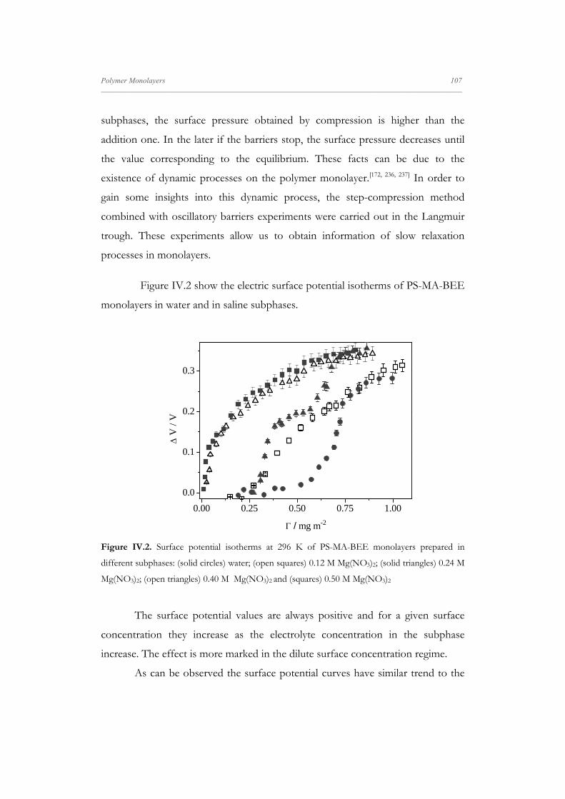
Polymer Monolayers 107 _____________________________________________________________________________________________________________________
subphases, the surface pressure obtained by compression is higher than the
addition one. In the later if the barriers stop, the surface pressure decreases until
the value corresponding to the equilibrium. These facts can be due to the
existence of dynamic processes on the polymer monolayer.[172, 236, 237] In order to
gain some insights into this dynamic process, the step-compression method
combined with oscillatory barriers experiments were carried out in the Langmuir
trough. These experiments allow us to obtain information of slow relaxation
processes in monolayers.
Figure IV.2 show the electric surface potential isotherms of PS-MA-BEE
monolayers in water and in saline subphases.
0.00 0.25 0.50 0.75 1.00
0.0
0.1
0.2
0.3
V
/ V
/ mg m-2
Figure IV.2. Surface potential isotherms at 296 K of PS-MA-BEE monolayers prepared in
different subphases: (solid circles) water; (open squares) 0.12 M Mg(NO3)2; (solid triangles) 0.24 M
Mg(NO3)2; (open triangles) 0.40 M Mg(NO3)2 and (squares) 0.50 M Mg(NO3)2
The surface potential values are always positive and for a given surface
concentration they increase as the electrolyte concentration in the subphase
increase. The effect is more marked in the dilute surface concentration regime.
As can be observed the surface potential curves have similar trend to the

108 Polymer Monolayers _____________________________________________________________________________________________________________________
surface pressure ones; thus, the surface potential isotherms are shifted to lower
surface concentration when the electrolyte concentration in the subphase
increases. The isotherm in 0.24 M Mg(NO3)2 shows a pseudo-plateau while it is
marked by a kink in the isotherms at lower electrolyte concentration in the
subphase. The plateau almost disappears when the monolayer is built in saline
subphases containing electrolyte concentrations above 0.4 M.
It is also interesting to notice that the surface potential at high surface
coverage does not increase with the electrolyte concentration for monolayers
containing high electrolyte concentration and the value remains constant in a
value of 0.35 V. This fact indicates that in these monolayers all acid groups are
dissociated.
Figure IV.3 presents the equilibrium elasticity modulus, 0, for different
polymer monolayers. The elasticity modulus is obtained from the pressure
isotherms.

Polymer Monolayers 109 _____________________________________________________________________________________________________________________
-0.2 0.0 0.2 0.4 0.6 0.80
20
40
0.0 0.5 1.0 1.5
0
20
40
0 /
mN
m-1
/ mg m-2
0 / mN m-1
/ mg m-2
Figure IV.3. Variation of the equilibrium elasticity with polymer surface concentration for
monolayers prepared in different subphases at 296K: (solid circles) water; (triangles) 0.12M
Mg(NO3)2; (open circles) 0.24 M Mg(NO3)2; (solid squares) 0.50 M Mg(NO3)2. The arrows point
polymer concentrations at which the kink in the surface potential isotherms appears. Solid and
open stars represent the dilational modulus obtained from step-compression experiments for
subphases containing 0.24 M Mg(NO3)2 and (solid squares) 0.50 M Mg(NO3)2, respectively, see
text.
Small elasticity values are observed for monolayers in water until the
surface concentration reaches a value of 0.8 mg m-2. A sudden increase of
elasticity is observed above this surface concentration until it reaches a value of 50
mN m-1. Finally, when the surface concentration is further increased a weak
decrease of the elasticity is observed. This behaviour is characteristic of films
formed exclusively by polymer molecules at concentrated regime. In these
concentrated films the conformational degrees of freedom of the polymer coils
decrease and consequently, the elasticity modulus also decreases.[172, 222] It is also

110 Polymer Monolayers _____________________________________________________________________________________________________________________
interesting to notice that the equilibrium elasticity modulus values are consistent
with liquid-expanded surface states [123] in all these monolayers. On the other
hand, and because the isotherms obtained by compression do not correspond to
the equilibrium ones (isotherms prepared by addition), the elasticity values
calculated from the isotherm obtained by compression are far from the
equilibrium elasticity values, see Figure IV.3.
Differences between the elasticity modulus of monolayers in saline and in
the unsalted subphases are the following: on the one hand, the equilibrium
elasticity values for dilute monolayers (Γ < 1 mg m-2) are higher for monolayers in
saline subphase than in the subphase without salt. The effect is more marked
when the salt concentration increases. An on the other hand, the equilibrium
elasticity curves for monolayers in saline subphases with salt concentrations below
0.4 M, present a kink or a plateau at the same surface concentration values than in
the surface potential curves. For comparative purposes the arrows in Figure IV.3
point to the position of the pseudo-plateau in the surface potential isotherms,
Figure IV.2.
The surface potential and pressure isotherms of PS-MA-BEE clearly
show that the monolayers become more expanded when the Mg(NO3)2
concentration in the subphase increases until it reaches a value of 0.4 M. Above
this concentration the isotherm remains unaffected by the increase of electrolyte
concentration. This behaviour could be attributed to the formation of a complex
between the divalent cation Mg2+ and the acid groups of the polymer molecules.
The isotherm expansion was observed by other authors when metal-surfactant
complexes are formed at the interface and the surfactant contains bulky head
groups.[238] This could be the scenario in our system because the hydrophilic part
of the polymer is too bulky and some molecular rearrangements have to be
carried out in order to form the complexes between the divalent cation and the
carboxylic groups of the polymer. Results also show that the isotherm expansion

Polymer Monolayers 111 _____________________________________________________________________________________________________________________
stop when the Mg(NO3)2 concentration in the subphase reaches a value of 0.4 M.
This fact indicates that at this salt concentration all the polymer molecules are
bound to the divalent cation.
The coincidence between the kink and the plateau positions observed in
the surface potential and the equilibrium elasticity isotherms may be indicative of
phase transitions that in this system can be originated by different populations of
free and bound polymer molecules. Accordingly, the plateau disappears when the
cation-polymer complexes at the interface predominate, [Mg(NO3)2] ≥ 0.4 M.
Dynamic Properties of Polymer Monolayers. As was previously mentioned,
the polymer isotherms obtained by continuous addition and compression agree
with each other when the surface concentration is relatively low. This behaviour
can be signature of dynamic processes on the monolayer. To study these
processes we have used the step-compression method.[222] In this method, the
monolayer is perturbed by a quick compression, and then the relaxation to the
new equilibrium condition is followed by surface pressure measurements.
Previously, we also use oscillatory barrier measurements to check the strain range
where the amplitude of the stress, σ0, is proportional to the strain, U0, the linear
regime. Examples of oscillatory experiments are presented in Figure IV.4 and
performed at a frequency of 0.006 Hz. For the sake of clarity Figure IV.4 shows
the results obtained for two different subphases, water and 0.24 M Mg(NO3)2.

112 Polymer Monolayers _____________________________________________________________________________________________________________________
3.0
3.5
4.0
0 1000 2000 3000 4000 5000
2.5
5.0
7.5
(t)
/ m
N m
-1
(t)
/ m
N m
-1
time / s
a
2.0
2.5
3.0
0 500 1000 1500 2000
2
4
6
(t)
/ m
N m
-1
b
time / s
(t)
/ m
N m
-1
Figure IV.4. Oscillatory experiment results at 296 K for different monolayers: (a) pure water and
polymer surface concentration around 0.9 mg m-2; (b) 0.24 M Mg(NO3)2, and polymer surface
concentration around 0.42 mg m-2. The strain amplitude was 4.3 % (solid circles) and 12 % (open
circles). The experiments were carried out at the frequency of 0.006 Hz.
As can be seen in Figure IV.4a for monolayers deposited on water

Polymer Monolayers 113 _____________________________________________________________________________________________________________________
subphase, after each compression-expansion cycle, the former initial state is not
recovered and the pressure decreases after each cycle. The amplitude of the stress
remains almost constant at low strains while it decreases at high strains. This
behaviour is not observed in monolayers prepared in saline subphases and can be
explained by developing of irreversible features in the film as it is strained by
subsequent compression-expansion cycles. This behaviour has been observed in
other polymer monolayers [130]; however, this fact could be simply due to the
desorption process followed by the polymer dissolution in the subphase. To
disregard this possibility we carried out the following experiment: a polymer
monolayer prepared by addition was submitted to compression-expansion cycles,
then the barriers were stopped and the pressure monitored with time (2 h). The
surface pressure decrease was least of 1%. Similar results were obtained at
different surface coverage. This observation is compatible with no polymer
dissolution in the subphase when the monolayer is strained.
Moreover, we carried out several oscillation barriers experiments changing
the cycle frequency from 0.003 to 0.04 Hz. For the case of polymer monolayers in
water subphase the surface pressure decreasing varies with frequency. The initial
state of the monolayer is not recovered, decreasing the surface pressure in a more
marked way when the frequency decreases. It could confirm the formation of
irreversible features in the film mainly at slow timescale. However in the case of
saline subphases the response amplitude does not show relevant changes with
frequency. Therefore, we decided to work at a slow suitable frequency for the
times of the processes involved, 0.006 Hz, which at the same time, is not affected
by the hydrodynamic limitations of the technique.
As we are interested in studying the relaxation process of polymer
monomers adsorbed in the monolayer, we have only studied the dynamic
processes on the monolayers prepared on saline subphases. Figure IV.5 presents
the variation of the amplitude of the stress σ0 with the strain, U0 for monolayers in

114 Polymer Monolayers _____________________________________________________________________________________________________________________
saline subphases. As can be seen in the figure, deviations of the Hookean linear
behaviour are observed for the area change above 10% of the total area.
Consequently, in the step-compression experiments the area change, ΔA, is kept
below 10% in order to ensure that the system remains in the linear regime. This
nonlinear behaviour has been found for other polymer monolayers.[128, 223]
0.0 0.1 0.20.0
2.5
5.0
7.5
0 / m
N m
-1
U0
Figure IV.5. Variation of the amplitude of the stress, σ0, with the strain, U0 for polymer
monolayers prepared in 0.12 M Mg(NO3)2 subphase (triangles) and in 0.24 M Mg(NO3)2 (circles).
The dot lines represent the Hookean’s linear behavior.
Stress-relaxation experiments show that in the low-coverage region, before
the end of the kink or the pseudo-plateau in the isotherms, the stress-relaxation
curve can be described by a single exponential function, Figure IV.6. However,
when the surface coverage is further increased no single-exponential relaxations
are found, this fact is indicative of additional processes in the monolayer. In
monolayers prepared in the most concentrated saline subphases, Mg(NO3)2 ≥ 0.4
M, the stress-relaxation curves are single-exponential functions for surface
concentrations below 1 mg m-2. Above this surface concentration no single-
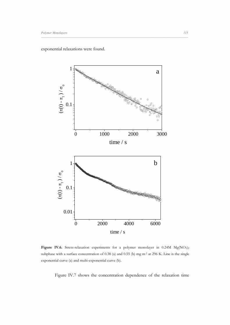
Polymer Monolayers 115 _____________________________________________________________________________________________________________________
exponential relaxations were found.
0 1000 2000 3000
0.1
1
((t
) - f )
/ 0
time / s
a
0 2000 4000 6000
0.01
0.1
1
((t
) -
f ) / 0
time / s
b
Figure IV.6. Stress-relaxation experiments for a polymer monolayer in 0.24M Mg(NO3)2
subphase with a surface concentration of 0.38 (a) and 0.55 (b) mg m-2 at 296 K. Line is the single
exponential curve (a) and multi-exponential curve (b).
Figure IV.7 shows the concentration dependence of the relaxation time

116 Polymer Monolayers _____________________________________________________________________________________________________________________
obtained for different monolayers. For the sake of clarity only some results are
presented in Figure IV.7. As can be seen in the figure different trends are found.
For monolayers in saline subphases with salt concentrations below 0.4 M, at low-
coverage, before the kink or the pseudo-plateau, the relaxation time increases with
the polymer concentration, this behaviour is characteristic of slow collective
motions of the polymer coils adsorbed at the interface[130, 238]. Conversely, at high-
coverage the relaxation time decreases when the polymer surface concentration
increases. According to the equilibrium properties, these surface concentrations
correspond to regions in the isotherm in the phase transitions. Consequently, the
concentration dependence of the relaxation time is a further indication of a
possible phase transition between a state in which we have polymer molecules
bound to the Mg2+ and a state with free polymer molecules.
On the other hand, when monolayers are prepared in subphases
containing electrolyte concentrations above 0.4 M, the stress-relaxation
experiments have led to relaxation curves described by a single exponential in the
surface concentration range between 0.15 and 1 mg m-2 and the relaxation time
increases with the surface concentration. As can be seen in Figure IV.7, the
relaxation time values are quite similar to those obtained for monolayers in 0.24 M
of Mg(NO3)2 at low surface coverage.

Polymer Monolayers 117 _____________________________________________________________________________________________________________________
0.2 0.4 0.60
500
1000
1500
/ mg m-2
/ s
Figure IV.7. Variation of the relaxation time with the polymer surface concentration for
monolayers prepared in the following subphases at 296K: (open circles) 0.12 M Mg(NO3)2; (solid
circles) 0.24 M Mg(NO3)2 and (open triangles) 0.50 M Mg(NO3)2. The arrows point polymer
concentrations at which the kinks in the surface potential and equilibrium elasticity isotherms
appear.
We have also determined the dilatational modulus, ||, from the
relaxation curves as 0
0
U
. Some of these values are represented in Figure IV.3
by stars. For the sake of clarity we only represent the values for monolayers in
subphases with 0.24 M and in 0.5 M of Mg(NO3)2. Results in Figure IV.3 show
that in the monolayers prepared in the subphase containing Mg(NO3)2 0.24 M,
there is an excellent agreement between the dilatational modulus and the
equilibrium elasticity at low-coverage. However, when the coverage increases the
dilatational modulus is higher than the equilibrium elasticity, this is indicative of
viscoelastic behaviour. The crossover between the elastic and viscoelastic
behaviour appears at the polymer surface concentration where deviations between
the isotherms obtained by addition and compressions become important. This
behaviour is observed for all monolayers with electrolyte concentrations below 0.4
118 Polymer Monolayers _____________________________________________________________________________________________________________________
M; however, when the electrolyte concentration in the subphase increases,
[Mg(NO3)2] ≥ 0.4 M, the dilatational modulus values are always higher than the
equilibrium elasticity ones. The differences between dilatational and equilibrium
elasticity values are quite marked. This fact indicates that the formation of
complexes between the polymer and the divalent cation increases the viscoelastic
behaviour of the monolayer.
As was indicated above the stress-relaxation experiments in the densest
monolayers have led to relaxation curves described by no single-exponential
curves in the densest monolayers. This behaviour can signify additional processes
such as disorder-order transitions [128] or polymer aggregation. To disregard this
point we transfer polymer monolayers from the liquid interface to mica and/or Si
(100) via the Langmuir-Blodgett technique (LB) because several studies showed
that aggregates produced by self-assembly monolayers can survive when are
transferred from the Langmuir monolayer to solid supports.[239-241] AFM results
show that the morphology of the polymer LB films is similar in mica and silicon
when the subphase is water, Figure IV.8. However, when the subphase contains
electrolytes both, AFM and optical microscopy show the formation of magnesium
salt crystals, Figure IV.9. Therefore, we decide to use silicon as substrate for the
polymer films study.

Polymer Monolayers 119 _____________________________________________________________________________________________________________________
Figure IV.8. AFM images of the LB films on mica (a) and Si (100) (b) for PS-MA-BEE
monolayers in water subphase at surface pressure 14 mN m-1 by compression.
Figure IV.9. Optical microscopy image of the Mg(NO3)2 crystals formed on mica after the LB
deposition of a polymer film prepared on saline subphase.
For comparative purposes we have also constructed LB films from Langmuir
monolayers at low surface coverage, below the end of the kink (in the pseudo
plateau). The AFM images show no domains in these LB films. However, the first
aggregates were clearly observed at the end of the pseudo-plateau, Figure IV.10.
0 100 200 300 400 5000
8
16
Z /
nm
X / nm0 100 200 300 400
0
8
16
Z /
nm
X / nm
a b

120 Polymer Monolayers _____________________________________________________________________________________________________________________
Figure IV.10. AFM image of the LB film on Si (100) for PS-MA-BEE monolayer in Mg(NO3)2
0.12M at surface pressure 4 mN m-1 (end of pseudo-plateau) by compression.
According to the differences observed in the properties of Langmuir films
prepared by addition and by compression, we build the LB films by transferring
Langmuir films prepared by the two different methodologies. Different
mesoscopic structures are detected as a function of the methodology used. To
illustrate this fact several AFM images are collected in Figure IV.11. We have
checked the reproducibility of the transfer procedure by obtaining each LB film at
least three times. The results agree with each other except for LB films built by
transferring the Langmuir film prepared by addition in a water subphase.
0 100 2000
2
4
Z /
nm
X / nm

Polymer Monolayers 121 _____________________________________________________________________________________________________________________
Figure IV.11. AFM images of the LB films on Si (100) for different PS-MA-BEE monolayers: in
water subphase at surface pressure 14 mN m-1 and 0.12M Mg(NO3)2 at 10 mN m-1, by subsequent
additions (a, c) and by compression (b, d), respectively. Below are the corresponding cross section
profiles. In addition the green angle pairs correspond to the angles pairs in the Figure 12c.
Images in Figure IV.11 clearly show different structures as a function of
both, the subphase composition and the methodology employed to prepare the
Langmuir monolayer which serve to build the LB films. Thus, when the Langmuir
monolayer was prepared in aqueous subphase by compression, long stripes are
observed, Figure IV.11b. These aggregates present a high degree of
reproducibility. In contrast, aggregates with different morphologies are observed
when the Langmuir monolayer is obtained by addition in water subphase, Figure
700nm 1.0µm
0 200 400048
12
Z /
nm
X / nm
400nm460nm
0 100 2000246
Z /
nm
X / nm
a b
c d
0 200 4000246
Z /
nm
X / nm
0.0 0.5 1.00
1
2
Z /
nm
X / nm
122 Polymer Monolayers _____________________________________________________________________________________________________________________
IV.11a. In this case the morphology of these aggregates also changes when the
polymer concentration of the spreading solution changes. This behaviour is
consistent with results obtained in previous work for diblock copolymers with
immiscible blocks confined to the surface.[242] A theoretical model has been
proposed to interpret this fact.[237] The model considers that the fast evaporation
of the spreading solvent and the extremely low solubility of the hydrophobic
blocks compared with the hydrophilic ones are the main reasons of the
association in metastable aggregates.
In the case of stripes, Figure IV.11b, the formation of this type of 2D
nanostructures has been previously observed and interpreted by spinodal
dewetting mechanism.[243-245]. A detailed discussion of this mechanism is presented
in Chapter V.
Figures IV.11c and d, show images of LB films built from dense Langmuir
monolayers in saline subphases 0.12M of Mg(NO3)2 prepared by addition and by
compression methodologies, respectively. Even though the morphology of
aggregates acceptably agrees with each other, differences in the monodispersity
degree can be observed. Thus, LB films built by transferring Langmuir films
prepared by compression are almost monodisperse and the average value of the
roughness is around 5 nm. In contrast, the LB prepared by addition show higher
polydispersity degree and the roughness values are between 3 and 5 nm. Finally, it
is interesting to notice that results in saline subphases obtained by the two
methodologies are reproducible.
Although the images in Figure IV.11c and d correspond to LB films built
with Langmuir films in 0.12 M Mg(NO3)2 subphase; similar images are observed
for the rest of films prepared in saline subphases. From the AFM results it is
possible to conclude that aggregates transferred from the concentrated
monolayers of polymer have different morphology than the ones transferred from
monolayers containing polymer-cation complexes.

Polymer Monolayers 123 _____________________________________________________________________________________________________________________
Finally, we have also used a laser ellipsometer to obtain the layer thickness
of the different LB films. In order to obtain the film thickness, different
approaches have been used to model the interfaces. We have modelled these films
as three layers: the first one is the Si substrate with a refractive index of 4.1264;
the second layer is the native oxide layer of a refractive index of 1.4653.[242] The
thickness of this layer was obtained in an ellipsometry experiment using the clean
silicon wafer. Finally, the third layer (polymer film/air) thickness and the
refractive index are obtained from the fitting of the two ellipsometric angles, Ψ,
and Δ, to Fresnel equation. Results obtained are collected in Table IV.1. From
data in Table IV.1 it is possible to conclude that the thickness values obtained by
ellipsometry are in good agreement with the average roughness of films obtained
by AFM measurements.
Table IV.1. Thickness and roughness values obtained from Ellipsometry and AFM measurements
of different PS-MA-BEE LB films deposited onto silicon wafers, respectively.
Subphase π /mN m-1 LB Method Roughness
AFM (nm)
Thickness Ellipsometry
(nm)
Water 14 Addition 1.5 – 2.5 2.5 ± 0.7
14 Compression 8.0 ± 0.6 8.1 ± 2.4
Mg(NO3)2
0.12 M
3.8 Addition 1.0 ± 0.5 1.8 ± 0.5
10 Addition 3-5 2.9 ± 0.8
10 Compression 5.0 ± 0.5 4.4 ± 1.3
IV.2. PS-b-MA Monolayers
In order to check the functional group by which the PS-MA-BEE forms
the complex with the Mg2+, we decide to compare this behaviour with another
maleic anhydride polymer, PS-b-MA, that is also a styrene/maleic anhydride
derivative. This polymer does not present a block with the carboxylic group,
which could be responsible for the formation of a complex in the case of PS-MA-

124 Polymer Monolayers _____________________________________________________________________________________________________________________
BEE monolayers between the COO- and Mg2+.[79] Thus, the aim of this brief work
is to confirm the effect of the polymer structure on the film properties.
Equilibrium Properties. Surface pressure vs surface concentration
isotherms on water and Mg2+ (0.12 M) aqueous subphases were prepared by
equilibration after each addition and by continuous compression. In this case, the
behaviour observed is opposite. As it is shown in Figure IV.12a, the isotherm
shifts to higher surface concentration when ions are added into subphase, i.e., the
isotherm is more condensed. This behaviour is in agreement with the lack of
interactions between the functional groups of PS-b-MA and the magnesium
cation, reinforcing that the effect observed on PS-MA-BEE is due to a Mg2+-acid
group complexation.

Polymer Monolayers 125 _____________________________________________________________________________________________________________________
1 2 30
10
20
/ m
N m
-1
/ mg m-20.5
a
0 1 2 30
10
20
30
0.5 1.0 1.50
50
100
0 / m
N m
-1
/ mg m-2
b
0 / mN m-1
/ mg m-2
Figure IV.12. Surface pressure (a) and equilibrium elasticity (b) isotherms of PS-b-MA
monolayers prepared in different subphases: (circles) water; and (squares) 0.12M Mg(NO3)2.
Surface isotherms were obtained by addition (symbols) and by symmetric compression (dot-solid
lines) at 293K.

126 Polymer Monolayers _____________________________________________________________________________________________________________________
On the other hand, LB depositions of the monolayers were made for the
different subphases to observe the influence of polymer structure and the
subphase on the aggregates obtained. The Langmuir monolayers were deposited
at a surface pressure of 10 mN m-1 on water and Mg2+ 0.12M aqueous subphases
at 20ºC onto silicon wafers. At this surface pressure the monolayer is the state that
corresponds to the maximum elasticity value, Figure IV.13b, as in the case of PS-
MA-BEE at π=14 mN m-1. AFM images for PS-b-MA show the same type of
aggregates (Figure IV.13) independently of the type of subphase. In this case, the
polymer forms enough homogeneous circular aggregates of 3-4 nm height and
~100 nm radius, Table IV.2, that could be attributed to plane/starfish or nanodot
surface micelles observed for other authors on polystyrene derivates at the air-
water interface [246-248] and they would be promoted by polystyrene block. In fact,
the surface micelle formation is based on the aggregation of hydrophobic blocks
to form an isolated phase of various shapes and it is stabilized by the corona of
hydrophilic blocks spread on the water surface.[246] Moreover, the observation of
surface micelles is in agreement with theoretical models proposed for
morphologies of the structures formed by block copolymers.[249] In this case, the
ratio between PS and MA blocks (number of monomers in each block, Ni,
NPS~15 and NMA~5) at low grafting density would lead to spherical interspersed
micelles. Likewise, as there are not interactions between the functional groups of
PS-b-MA and magnesium cation, the structure is kept.

Polymer Monolayers 127 _____________________________________________________________________________________________________________________
Figure IV.13. AFM images of a LB films on Si (100) for a PS-b-MA monolayers in water (a) and
0.12M Mg(NO3)2 aqueous subphase (b) at surface pressure 10 mN m-1 by compression with its
corresponding cross section profile.
Table IV.2. Average values of the dot-like feature dimensions formed in PS-MA-BEE and PS-b-
MA LB films deposited at a surface pressure of 10 mN m-1 obtained from AFM measurements.
Polymer Subphase Diameter / nm
PS-b-MA Water 121 ± 43
Mg(NO3)2 0.12 M 95 ± 32
PS-MA-BEE Mg(NO3)2 0.12 M 55 ± 10
Reported values are averages and error represents the standard deviation determined from at least
40 surface features.
Besides, ellipsometric measurements, collected in Table IV.3, were carried
out in order to confirm the roughness obtained by AFM profiles by applying the
same interface model as in the case of PS-MA-BEE.
Table IV.3. Thickness and roughness values obtained from Ellipsometry and AFM measurements
of different PS-b-MA LB films deposited at the surface pressure of 10 mN m-1 by symmetric
compression onto silicon wafers, respectively.
Subphase Roughness AFM (nm) Thickness Ellipsometry (nm)
Water 3.5 ± 0.5 4.3 ± 1.2
Mg(NO3)2 0.12 M 4.0 ± 0.5 5.0 ± 1.4
0 1 2024
Z /
nm
X / m0 200 400 600
0
2
4
Z /
nm
X / nm
a b

128 Polymer Monolayers _____________________________________________________________________________________________________________________
In previous work of the group [172], the soft-glass transition of two maleic
anhydride derivative polymers, PMAO and PS-b-MA, were observed by surface
potential measurements and confirmed by rheological measurements, both at the
air-water interface. From these results, the 2D glass transition temperatures were
determinated at 27ºC (300K) for PS-b-MA and 22ºC (295K) for PMAO. In order
to check the effect of the electrolytes presence on the water subphase, we carry
out surface potential measurements by temperature variation of PS-b-MA
monolayers on Mg2+ (0.12 M) subphase. For comparison the measurements were
carried out at the overlap surface pressure as in the case of water subphase.[172]
Results in Figure IV.14 show that surface potential increases when decrease the
temperature due to a restriction of the hydrophobic chains movements promoting
a higher orientation in the monolayer highlighted with the potential surface
increasing.[250] This fact indicates that the glass state is highly ordered due to
intermolecular interactions between the molecules that forms the glass phase.
290 295 300 305
1
2
FLUID STATE
V
/V
F
T / K
GLASS STATE
Tg
Figure IV.14. Surface potential variation with temperature for monolayers of PS-b-MA on water
(circles) and Mg(NO3)2 (squares) subphases. The surface potential values are normalized to the
final one, ΔVF.
Accordingly, the surface potential measurements show a change in the
orientation of the molecules at the temperature of 299.5±0.5K, the 2D glass

Polymer Monolayers 129 _____________________________________________________________________________________________________________________
transition temperature. Besides, this temperature is not significantly modified with
the addition of salts on the water subphase. The most significant difference is the
slope of the surface potential in the glass state in the presence of Mg2+. This
behaviour could be ascribed to a more perpendicular orientation of the dipole
induced by the ions.[79]
In the case of PS-MA-BEE the surface potential measurements did not
allow to observe the 2D glass transition temperature. This picture could be due to
different chain flexibility as indicate the bulk glass transition temperature: PS-MA-
BEE (76ºC, 349K) and PS-b-MA (122ºC, 395K) measured by DSC, Figure IV.15.
The chain mobility is related to the greater flexibility of the different units that
form the chain, thus a greater flexibility more chain mobility and lower glass
transition temperature.[251] Accordingly, it is not possible to observe the 2D glass
state for the PSMABEE at the air-water interface because usually this temperature
is around 100 degrees below the bulk glass transition temperature.[222] This 2D Tg
reduction in adsorbed films with respect to bulk polymers can be attributed to the
decrease of the intermolecular interactions due to the reduction of one
dimensionality.[252] Therefore, the surface potential values point out to the chain
orientation as an important factor.
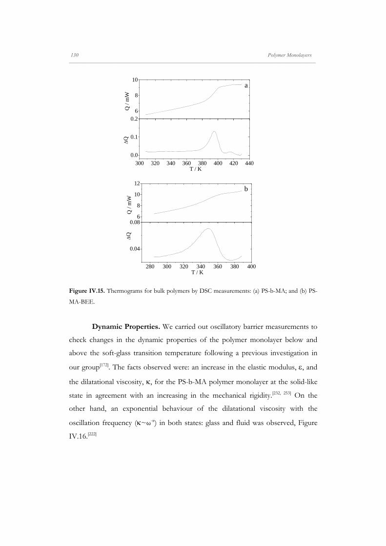
130 Polymer Monolayers _____________________________________________________________________________________________________________________
6
8
10
Q /
mW
a
300 320 340 360 380 400 420 440
0.0
0.1
0.2
T / K
Q
6
8
10
12
Q /
mW
b
280 300 320 340 360 380 400
0.04
0.08
T / K
Q
Figure IV.15. Thermograms for bulk polymers by DSC measurements: (a) PS-b-MA; and (b) PS-
MA-BEE.
Dynamic Properties. We carried out oscillatory barrier measurements to
check changes in the dynamic properties of the polymer monolayer below and
above the soft-glass transition temperature following a previous investigation in
our group[172]. The facts observed were: an increase in the elastic modulus, , and
the dilatational viscosity, , for the PS-b-MA polymer monolayer at the solid-like
state in agreement with an increasing in the mechanical rigidity.[232, 253] On the
other hand, an exponential behaviour of the dilatational viscosity with the
oscillation frequency (~ω-α) in both states: glass and fluid was observed, Figure
IV.16.[222]
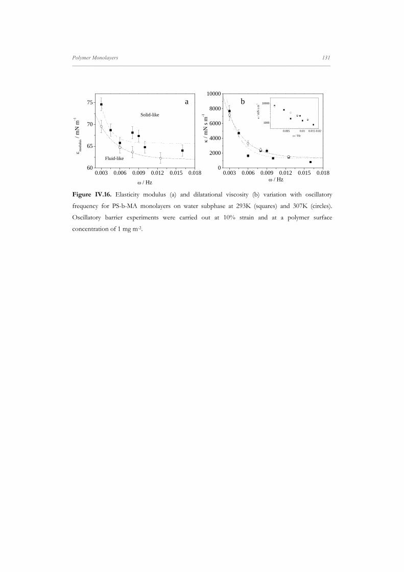
Polymer Monolayers 131 _____________________________________________________________________________________________________________________
Figure IV.16. Elasticity modulus (a) and dilatational viscosity (b) variation with oscillatory
frequency for PS-b-MA monolayers on water subphase at 293K (squares) and 307K (circles).
Oscillatory barrier experiments were carried out at 10% strain and at a polymer surface
concentration of 1 mg m-2.
0.003 0.006 0.009 0.012 0.015 0.01860
65
70
75
Fluid-like
mod
ulus
/ m
N m
-1
/ Hz
Solid-like
0.003 0.006 0.009 0.012 0.015 0.0180
2000
4000
6000
8000
10000
0.005 0.01 0.015 0.02
1000
10000
/ m
N s
m-1
/ Hz
/ m
N s
m-1
/ Hz
a b


V. Preparation and Properties of QDs Films


Preparation and Properties of Quantum Dots Films 133 _____________________________________________________________________________________________________________________
V. Preparation and Properties of QDs Films
Semiconductor quantum dots (QDs) have attracted much attention in
recent years owing to their unique chemical and physical properties [7] and their
applications as building blocks for photovoltaic,[254, 255] optoelectronic[256] or
magnetic devices,[257] and for selective recognition of ions[258] or biomedical
applications[259]. Inside the QDs, the hydrophobic nanoparticles present higher
quantum efficiency than the hydrophilic ones.[260] The current interest in the
fabrication of nanodevices is focused on the incorporation of QDs in well defined
layers and their immobilization onto solid substrates to obtain good quality
devices.[37, 51] In this sense the interfacial self-assembly is a selective method to
provide well-organized structures with controlled size and shape for the
fabrication of optoelectronic devices with QDs.
Moreover, the nanoparticle-polymer blend systems have shown potential
applications based on the modulation of the hybrid material properties to achieve
significant enhancements.[8] However, many nanofillers used in nanocomposites
tend to agglomerate by attractive interactions[153, 261] decreasing the quality of
nanocomposites. Therefore, the most recent efforts involve the use of polymer or
surfactant molecules to minimize filler agglomeration. Despite the great interest
aroused in the last years, more work must be carried out to develop
multifunctional materials with novel electric, magnetic or optical properties.[63, 262,
263]
An important issue concerning the properties of filler deposited on solids is
to achieve control over the organization and assembly of nanoparticles at
interfaces. Many techniques have been used to achieve good-quality
nanocomposites.[264-266] For hydrophobic nanoparticles an effective method to
produce well-defined QDs monolayers could be the Langmuir-Blodgett technique
(LB). The LB methodology (LB) has been proposed as a platform that renders the
self-assembly process of different hydrophobic nanomaterials at the air-water

134 Preparation and Properties of Quantum Dots Films _____________________________________________________________________________________________________________________
interface under well controlled and reproducible conditions.[1, 2] Therefore, it
offers the possibility of preparing polymer and nanoparticle reproducible films
with the control of the interparticle distance necessary to exploit the
nanocomposites in technological applications. In addition, the dewetting
processes observed in the preparation of LB films can be employed to achieve
patterning without a defined template. Despite the above mentioned advantages,
when the hydrophobic nanoparticles were transferred from the air-water interface
onto glass, silicon or mica substrates without treatment to become the solid
surface hydrophobic, low coverage and nanoparticle agglomeration have been
observed in LB films.[69, 140] To solve this problem some authors have proposed
two approaches. In the first one, mixed Langmuir films of surfactants[67, 146-149] or
polymers[14, 15, 148, 267] and hydrophobic nanoparticles are transferred from the air-
water interface onto solid substrates by the LB method. This approach seeks to
control the assemblage of hydrophobic nanoparticles on water. In the case of
polymers, if the polymer is an amphiphilic block copolymer, the most hydrophilic
block can favour the nanoparticles spreading and the adsorption on the solid
avoiding the 3D aggregation. Moreover, because block copolymers can aggregate
at the interface[59, 63], the self-assembly of nanoparticles on these copolymers can
be proposed as a way to organize hybrid materials at nanometre scale[13, 267, 268]. The
second methodology proposed is the interchange of the stabilizer ligand, TOPO,
by thiols [269], alkylamines [270], alkylphosphoramines [7] and block copolymers [14, 150,
271, 272]. Even though some improvements have been achieved with this
methodology, the appropriate control of the self-assembly process remains still a
challenge. Despite the successful results reported, more efforts must be carried
out to develop nanometric structures that may provide new phenomena
associated with the size reduction of materials.[147] Thus, major advances in the
field of self-assembly must be made in order to achieve a better understanding of
the process to make use of the functionality offered by nanomaterials and to
improve their practical applications.
Preparation and Properties of Quantum Dots Films 135 _____________________________________________________________________________________________________________________
With this objective in mind, we focus our interest on the self-assembly of
CdSe QDs onto solid substrates assisted by the block copolymer PS-MA-BEE.
We choose this polymer because it self-assembly at the air-water interface at a
given polymer surface concentration.[273] Therefore, as polymer assembly modifies
the surface properties[274-277] it provides us an excellent way to study the role of the
surface properties of the precursor Langmuir monolayer on the LB film
architecture and photoluminescence properties. On the other hand,
styrene/maleic anhydride copolymers have shown potential application in optical
waveguides, electron beam resists and photodiodes.[5, 6] Therefore, it could be a
good candidate to prepare hybrid materials for optoelectronic devices
fabrication.[13, 267, 268]
To assist the QDs self-assembly, we use the polymer PS-MA-BEE in three
different ways. In the first strategy, we use the polymer as matrix to assist the
QDs self-assembly at the air-water interface. Thus, a QD/PS-MA-BEE mixed
Langmuir monolayer is transferred by the LB method onto the solid. In the
second one, a LB film constructed by the polymer PS-MA-BEE is used as coating
for the substrate to deposit the QDs Langmuir films. Here the polymer was used
in order to control the QDs adsorption on the solid. We use this polymer because
spreads well onto the substrates used. The presence of the polymer on the solid
essentially modifies the surface properties of the substrate and could allow tuning
the QDs film properties. In the third approach, the QD stabilizer, TOPO, is
exchanged by the polymer to analyze the effect of the ligand on the modulation of
self-assembly at the air-water interface. This polymer contains a free carboxylic
acid group that can interact with the Cd2+ localized in the surface of the QD
core.[8] The assemblies obtained with these QDs are transferred by the LB
methodology onto the solid wafer.
Accordingly, this chapter is organized in three parts. In the first one, we
prepare the LB films by the proposed strategies and study the different film

136 Preparation and Properties of Quantum Dots Films _____________________________________________________________________________________________________________________
morphologies by means of atomic force microscopy (AFM) and transmission
electron microscopy (TEM). Previously, we carried out the characterization of the
Langmuir monolayers which serve as precursors of the LB films by performing
the surface-pressure isotherms and by obtaining images of the monolayers using
the Brewster Angle Microscopy (BAM).
In the second part of the chapter, the dynamic properties of mixed
Langmuir films of PS-MA-BEE and QDs were studied. This part has a double
objective. On the one hand, the study of the influence of the shearing on the
QD/PS-MA-BEE film morphology and on the other hand, to analyze the
dynamic processes involved in the reorganization of the monolayers after shearing
due to the knowledge of the dynamic properties of these nanocomposites is
essential in order to guarantee the processability, reliability and stability of
QD/polymer devices.[17] In this sense, the effect of the mixture composition is
also investigated.
Finally, as the QDs emission can be used to fabricate LEDs, the
fluorescence properties of the QD films were studied analyzing the effect of the
self-assemblies morphology on the QD emission properties. This
photoluminescence characterization was performed by means of Fluorescence
Lifetime Imaging Microscopy (FLIM).
V.1. Experimental Section
In this section the synthesis, extraction and size characterization of the
TOPO-capped CdSe QDs used in this work is briefly presented.
The hydrophobic QDs were synthesized by the method proposed by Yu
and Peng.[278] This method uses cadmium oxide and selenium powders as
precursors. Firstly, a selenium precursor solution was prepared by mixing Se
(0.030 g), TOP (0.4 mL) and octadecene (5 mL). The solution is stirred and
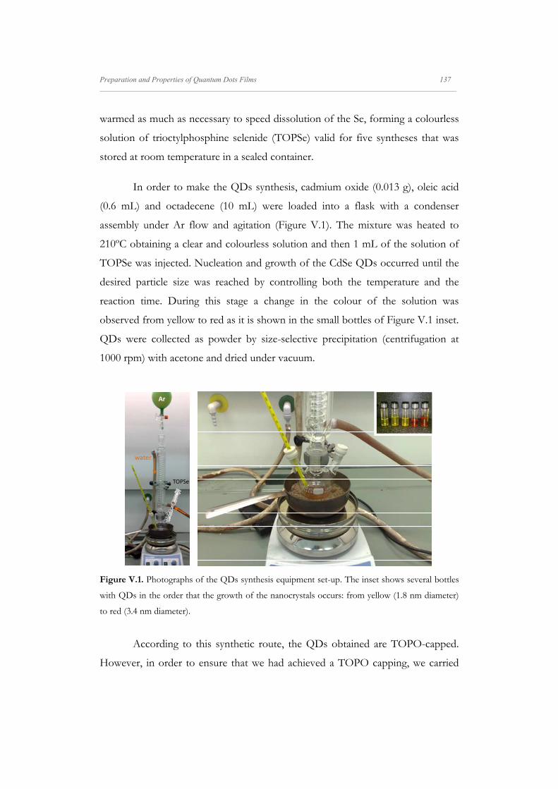
Preparation and Properties of Quantum Dots Films 137 _____________________________________________________________________________________________________________________
warmed as much as necessary to speed dissolution of the Se, forming a colourless
solution of trioctylphosphine selenide (TOPSe) valid for five syntheses that was
stored at room temperature in a sealed container.
In order to make the QDs synthesis, cadmium oxide (0.013 g), oleic acid
(0.6 mL) and octadecene (10 mL) were loaded into a flask with a condenser
assembly under Ar flow and agitation (Figure V.1). The mixture was heated to
210ºC obtaining a clear and colourless solution and then 1 mL of the solution of
TOPSe was injected. Nucleation and growth of the CdSe QDs occurred until the
desired particle size was reached by controlling both the temperature and the
reaction time. During this stage a change in the colour of the solution was
observed from yellow to red as it is shown in the small bottles of Figure V.1 inset.
QDs were collected as powder by size-selective precipitation (centrifugation at
1000 rpm) with acetone and dried under vacuum.
Figure V.1. Photographs of the QDs synthesis equipment set-up. The inset shows several bottles
with QDs in the order that the growth of the nanocrystals occurs: from yellow (1.8 nm diameter)
to red (3.4 nm diameter).
According to this synthetic route, the QDs obtained are TOPO-capped.
However, in order to ensure that we had achieved a TOPO capping, we carried
Ar
water
TOPSe

138 Preparation and Properties of Quantum Dots Films _____________________________________________________________________________________________________________________
out FTIR measurements with QD powder and TOPO, Figure V.2. The FTIR
spectrum of nanoparticles presents peaks matching the TOPO spectrum, except
for the peak at 1144 cm-1 corresponding to the P=O stretch. It was demonstrated
that this peak is shifted between 20 and 60 cm-1 lower relative to bulk TOPO
upon complexation with CdSe.[279] Therefore, the peak centred at 1108 cm-1 in the
FTIR spectrum of QDs can be ascribed to the phosphonate molecules bound to
the nanoparticles surface. Thus, by comparing the QDs and TOPO FTIR spectra,
namely the P=O stretch frequency [280], we confirmed the presence of the
phosphonate ligand on the nanoparticle surface. Furthermore, latter studies
indicate that in similar syntheses [281] a thorough surface analysis reveals that the
nanoparticles are capped by octylphosphonate derivative ligands, which remain
bound to the surface (Cd2+ binding) after precipitation/washing steps.
1600 1400 1200 10000
20
40
60
80
100
CH3
Bend P-O Stretch
% T
/ a.
u.
wavenumber / cm-1
QDTOPO
TOPO
Figure V.2. FTIR spectra of TOPO and TOPO-capped QDs, (QDTOPO), dispersed in KBr. For
clarity, the %T-scale is shifted and the QDTOPO spectrum amplified.
The diameter of the QDs was determined by the position of the maximum
of the visible spectrum of the QDs dispersed in chloroform [204], Figure V.3. The

Preparation and Properties of Quantum Dots Films 139 _____________________________________________________________________________________________________________________
value found was (566 ± 1 nm) that corresponds to a nanoparticle diameter of
(3.41 ± 0.05 nm), the red solution bottle in Figure V.1 inset. The QD size selected
is the most controllable size in the synthesis used as the nanocrystal growth and
population is controlled by time. Therefore, by this synthesis the maximum
diameter, ca. 4 nm, and the greatest QDs population are achieved at longer times.
The concentration of nanocrystals was calculated from the UV-Vis absorption
spectrum of the QDs solutions by using the extinction coefficient per mole of
nanocrystals at the first excitonic absorption peak.[204] UV-Vis absorption spectra
were recorded on a Shimadzu UV-2401PC spectrometer, Figure V.3.
400 500 600 700
UV
-Vis
abs
orba
nce
(a.u
.)
/ nm
3.4 nm
2.8 nm
2.2 nm
Figure V.3. Normalized absorption spectra of several CdSe QDs solutions in chloroform. The
diameter of the nanoparticles is also indicated.
V.2. Preparation of QDs Films
V.2.1. Langmuir and Langmuir-Blodgett Films of QDs and PS-MA-BEE
The first strategy employed was to use the polymer as matrix to assist the
QDs self-assembly. Therefore, we transfer mixed Langmuir monolayers of

140 Preparation and Properties of Quantum Dots Films _____________________________________________________________________________________________________________________
TOPO-capped CdSe QDs and PS-MA-BEE from the air-water interface onto
mica. As small changes on the composition of a mixed monolayer modify the
structure of the film,[172, 174, 250, 282] we study the effect of the polymer concentration
on the surface properties of the Langmuir films precursors of the LB films. The
characterization of these mixed monolayers allows us to select monolayers with
very different surface properties and to transfer them onto mica, in order to
investigate the role of these properties on both, the morphology of QDs films and
the self-assembly process.
The surface properties of the Langmuir monolayers were studied by
recording the surface pressure-concentration isotherms of the pure components
and mixtures of QDs and polymer at different composition. According to results
presented in chapter IV, the LB films obtained by transferring PS-MA-BEE
Langmuir monolayers prepared by addition consist of metastable states. Thus, we
prepare the Langmuir monolayers by compression because this method renders
the most reproducible and stable LB films in the case of the polymer. Figure V.4a
shows the isotherms of different mixtures and pure components, QDs and PS-
MA-BEE.
In the case of mixed monolayers it is well established that their surface
properties depend on the spreading technique.[172, 283, 284] Therefore, we test the
isotherm properties of monolayers obtained by spreading both components at the
interface, named as co-spreading, or adding the components separately. In all
cases the isotherms were very stable. A representative example for mixed
monolayers of polymer mole fraction XP = 0.50 is presented in Figure V.4b.
Significant differences between the isotherms can be observed. Thus, from the
three spreading procedures the densest monolayer is that obtained by co-
spreading. This behaviour was observed in other systems [172, 283] and ascribed to
the existence of attractive interactions between polymer and QDs molecules in
the spreading solution [283]. As was demonstrated in our previous work,[172, 284] the

Preparation and Properties of Quantum Dots Films 141 _____________________________________________________________________________________________________________________
co-spreading method proved to be the most reproducible technique and
consequently, was chosen to build the mixed QD/PS-MA-BEE monolayers.
Figure V.4. (a) Surface pressure isotherms of mixed Langmuir monolayers of QDs and PS-MA-
BEE with polymer mole fraction of: 0.07 (1); 0.15 (2); 0.35 (3); 0.55 (4); 0.65 (5); 0.80 (6); 0.93 (7);
0.96 (8); 0.98 (9); 0.99 (10) and pure PS-MA-BEE. The inset shows the QDs surface pressure
isotherm. The dotted lines indicate the surface pressures for the LB deposition: 14 and 30 mN m-1.
(b) Surface pressure isotherms for QD/PS-MA-BEE mixed monolayers at polymer mole fraction
of 0.50 obtained with separate spreading of QDs and PS-MA-BEE (1) and PS-MA-BEE and QDs
(2), respectively, and co-spreading (3). (c) Equilibrium surface elasticity vs. surface pressure for
several mixed Langmuir monolayers of QDs and PS-MA-BEE at different polymer mole fraction:
QDs (closed triangles); 0.07 (open rhombi); 0.35 (closed rhombi); 0.55 (open triangles); 0.65
(stars); 0.96 (open circles); and PS-MA-BEE (closed circles). The dashed lines delimit the surface
pressures where the plateaux in the surface pressure isotherms appear. The isotherms were
recorded by symmetric barrier compression at 5 mm min-1 and 23ºC.
0
20
40
10.10.001
100
20
40
/ m
N m
-1
QDs
/ mg m-2
50
9
875431 2
/ m
N m
-1
PS-MA-BEE
/ mg m-2
PS-M
A-B
EE
6
QDs
0.01 0.1 0.20
20
40
3
2
/ m
N m
-1
PS-MA-BEE / mg m-2
1
a
b
c
0 10 20 300
20
40
60
0 / m
N m
-1
/ mN m-1
PS-MA-BEE
QDs

142 Preparation and Properties of Quantum Dots Films _____________________________________________________________________________________________________________________
The QDs and PS-MA-BEE isotherms agree with those reported
previously.[67, 273] In mixed monolayers, at high polymer concentration, XP ≥ 0.95,
the isotherms present a plateau at the surface pressure value of 30 mN m-1. This
plateau could be related to phase coexistence and has been previously observed in
other block-copolymer isotherms.[57, 285, 286] To gain insight into the states of the
monolayers we have calculated the equilibrium elasticity modulus, 0, from the
surface pressure isotherms. For the sake of comparison the elasticity values are
represented against the surface pressure values in Figure V.4c. These results show
that the monolayer elasticity increases with the surface pressure and reaches a
maximum at a given surface pressure. The maximum position is shifted to higher
surface pressures for mixed monolayers. Beyond the maximum, when the surface
pressure is further increased, the elasticity decreases and for monolayers with
surface compositions XP ≥ 0.95 the elasticity goes through a minimum at the
surface pressure value of 30 mN m-1. The region around the elasticity minimum
corresponds to the plateau in the surface pressure isotherm. For comparative
purposes dashed lines in Figure V.4c delimit the plateau region.
Comparison between the elasticity and surface pressure isotherms of the
polymer PS-MA-BEE with those reported for other Langmuir monolayers of
block copolymers allowed us to obtain information about the polymer states at
the interface. Results in the literature demonstrated that at low surface pressures
the polymer blocks presents an almost flat conformation without tails protruding
from the subphase, in this regime the elasticity increases with the surface
concentration until it reaches the maximum value. In this state the monolayer can
be formed by aggregates with different features.[57, 248, 286] As it is discussed next,
the polymer PS-MA-BEE aggregates in stripes. At surface pressures beyond the
elasticity maximum, the polymer hydrophilic blocks protrude into the water
subphase and the elasticity values decrease until a minimum at which the polymer
brush conformation predominates. In this region the aggregates coexist with
brush structures, and it corresponds to the plateau in the surface pressure

Preparation and Properties of Quantum Dots Films 143 _____________________________________________________________________________________________________________________
isotherms. In our system the phase coexistence is between stripes and brushes.
For surface pressures beyond the elasticity minimum, is generally admitted that
interactions between the polymer blocks lead to a further increase of the surface
elasticity.[285, 287]
For mixed QD/polymer monolayers, the morphology of the elasticity
curves, Figure V.4c, also depends on the surface composition. From results in
Figure V.4c, it is possible to notice that the minimum in the elasticity curve
appears for mixed monolayers with high polymer concentration, XP ≥ 0.95.
Taking into account that the elasticity minimum also appears in the polymer
monolayer and it was ascribed to the polymer brush state, the behaviour observed
in mixtures seems to indicate that the brush regime is only reached in mixed
monolayers with high polymer concentration.
To gain insight into the morphology of QD/PS-MA-BEE monolayers, we
use the Brewster Angle Microscopy (BAM). Several images corresponding to
monolayers at two surface pressure values, 14 mN m-1 and 30 mN m-1 and
different surface compositions are collected in Figure V.5. BAM images of
monolayers at 14 mN m-1 and low polymer concentration, Figures V.5a and b,
show QD agglomerates. However, when the polymer concentration increases, the
QD agglomeration decreases, Figures V.5c and d. This behaviour can be
interpreted if one considers that, in the absence or at low polymer concentration,
the interactions between water subphase and the QDs stabilizer, TOPO, are too
weak, and they promote the agglomeration of nanoparticles at the air-water
interface [143, 153]. However, when the polymer concentration increases, attractive
interactions between the polymer hydrophobic block and the alkyl chains of
TOPO favour the QDs spreading on the water surface across the polymer
hydrophilic blocks avoiding the QDs agglomeration.[67, 243, 244]

144 Preparation and Properties of Quantum Dots Films _____________________________________________________________________________________________________________________
Figure V.5. BAM images (800x600 μm) at 14 mN m-1 for different QD/PS-MA-BEE mixed
monolayers with different polymer mole fractions: (a) pure QDs; (b) 0.50; (c) 0.96 and (d) 0.98.
BAM image of QD/PS-MA-BEE mixed monolayer at 30 mN m-1 and at polymer mole fraction of
0.96 (e).
Monolayers with high surface coverage (π = 30 mN m-1) are constituted by
domains so close-packed that BAM images do not allow us to visualize details of
its morphology. As illustrative example, we present in Figure V.5e the BAM image
of the mixed monolayer at 30 mN m-1 and XP = 0.96.
The next step was to transfer the polymer Langmuir monolayers from the
air-water interface onto mica by using the Langmuir-Blodgett technique. The
monolayers were transferred at the surface pressure values of 14 and 30 mN m-1.
We chose these monolayers because correspond to representative states of the
polymer monolayer. Thus, the monolayer at the surface pressure of 14 mN m-1 is
far from the brush regime and corresponds to the most elastic surface state, while
the monolayer at 30 mN m-1 corresponds to the polymer brush regime, minimum
in the elasticity curve. For the sake of comparison, we have also transferred QDs
monolayers at the same surface pressure values, 14 and 30 mN m-1, onto mica
without polymer.

Preparation and Properties of Quantum Dots Films 145 _____________________________________________________________________________________________________________________
The AFM images of QDs films are collected in Figures V.6a and b. As can
be seen in Figure V.6a the QDs film is mainly constituted by QDs 3D
agglomerates of different sizes and when the surface concentration of the QDs
transferred was further increased until a surface pressure value of 30 mN m-1, the
density of agglomerates increases and even more 3D aggregates are formed. This
fact can be interpreted if one considers that due to the low affinity of the QDs
stabilizer TOPO and the solid mica, the nanoparticles do not spread well. This
favours the QD 3D agglomeration.
On the other hand, the AFM images of polymer LB films, Figures V.6c
and d, revealed that the films obtained at different surface densities have different
morphologies. Thus, the polymer aggregates in stripes with a height profile of ~8-
10 nm when the surface pressure of the Langmuir monolayer transferred on mica
is 14 mN m-1, Figure V.6c, [273] while films with domains separated by holes were
observed when the surface coverage increases until 30 mN m-1, Figure V.6d. The
domain height profile found was ~ 2 nm, which agrees with the polymer
thickness calculated by means of molecular mechanic MM2 calculations (2.1 nm).
In polymer LB films the existence of two different features depending on
the polymer concentration points to two distinct dewetting mechanisms. Thus,
stripes and other 2D structures were previously observed and interpreted by
spinodal dewetting mechanism.[243-245] While, domains separated by holes were
observed in films in which the gravitatory effects are important.[44] In an attempt
to interpret the different behaviour observed it was necessary to analyze the
driving forces involved in the surface arrangement. Taking into account that the
molecular weight of this polymer is too low, one expects that the gravitatory
effects were neglected; however, it is necessary to compare this effect with that of
the capillary waves. It is well established that the damping coefficient passes
though a maximum at low elasticity values [288] and decreases when the elasticity
modulus increases. Accordingly, in the case of the most elastic monolayer (π = 14

146 Preparation and Properties of Quantum Dots Films _____________________________________________________________________________________________________________________
mN m-1), the capillary effects could predominate against the gravitatory ones and
the dewetting mechanism is driven by the capillary waves resulting in films
constituted by stripes. Conversely, in less elastic monolayer (π = 30 mN m-1), the
capillary waves are quickly damped and the polymer film breaks in domains
separated by holes due to gravitatory effects. Consequently, the growth of holes
dewetting mechanism predominates against the spinodal one in this monolayer
state.
Figure V.6. AFM images of QDs (a, b) and PS-MA-BEE (c, d) LB films deposited at the surface
pressures values of (a, c) 14 mN m-1 and (b, d) 30 mN m-1.
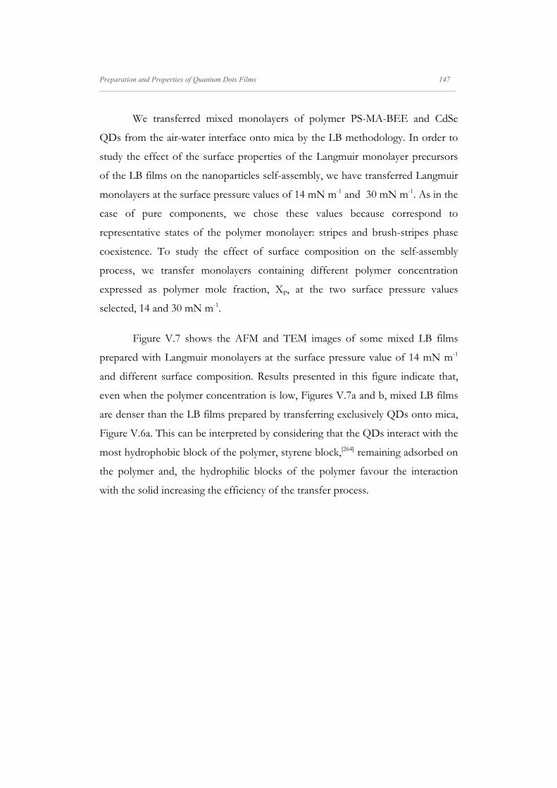
Preparation and Properties of Quantum Dots Films 147 _____________________________________________________________________________________________________________________
We transferred mixed monolayers of polymer PS-MA-BEE and CdSe
QDs from the air-water interface onto mica by the LB methodology. In order to
study the effect of the surface properties of the Langmuir monolayer precursors
of the LB films on the nanoparticles self-assembly, we have transferred Langmuir
monolayers at the surface pressure values of 14 mN m-1 and 30 mN m-1. As in the
case of pure components, we chose these values because correspond to
representative states of the polymer monolayer: stripes and brush-stripes phase
coexistence. To study the effect of surface composition on the self-assembly
process, we transfer monolayers containing different polymer concentration
expressed as polymer mole fraction, XP, at the two surface pressure values
selected, 14 and 30 mN m-1.
Figure V.7 shows the AFM and TEM images of some mixed LB films
prepared with Langmuir monolayers at the surface pressure value of 14 mN m-1
and different surface composition. Results presented in this figure indicate that,
even when the polymer concentration is low, Figures V.7a and b, mixed LB films
are denser than the LB films prepared by transferring exclusively QDs onto mica,
Figure V.6a. This can be interpreted by considering that the QDs interact with the
most hydrophobic block of the polymer, styrene block,[264] remaining adsorbed on
the polymer and, the hydrophilic blocks of the polymer favour the interaction
with the solid increasing the efficiency of the transfer process.

148 Preparation and Properties of Quantum Dots Films _____________________________________________________________________________________________________________________
Figure V.7. TEM (a, c) and AFM (b, d) images of mixed QD/PS-MA-BEE LB films deposited at
the surface pressure of 14 mN m-1. The film composition expressed as polymer mole fraction is:
0.35 (a, b); and 0.50 (c, d).
When the polymer concentration increased the film begins to break, see
Figures V.7c and d. Moreover, for polymer concentrations above XP > 0.5 the
QDs films presents the formation of domains distributed in islands, Figures V.8a
to c. Figure V.8d presents a high magnification AFM image of these domains,
showing that the islands are surrounded by polymer molecules. It is important to
note that the morphologies observed by AFM and TEM agree with each other
and that the domains height determined from AFM is independent of the polymer
concentration. The average height profile value of 4 nm is compatible with the
diameter of the QDs (3.41 ± 0.05 nm).
b
2.0µm
d
a
250 nm
c
0 1 2 30
4
8
Z /
nm
X / m
0 1 2 3 40
4
8
Z /
nm
X / m

Preparation and Properties of Quantum Dots Films 149 _____________________________________________________________________________________________________________________
Figure V.8. TEM (a, b) and AFM (c, d) images of mixed QD/PS-MA-BEE LB films deposited at
the surface pressure of 14 mN m-1. The film composition expressed as polymer mole fraction is:
0.65 (a); and 0.98 (b, c, d).
Our results also demonstrated that even when the QDs composition was
too small, the film morphology of QD/PS-MA-BEE mixed films is different to
that corresponding to the polymer PS-MA-BEE. This fact indicates that small
concentrations of QDs modify the interactions between the polymer molecules[289-
291] distorting the polymer film architecture.
To analyze the effect of the polymer concentration on the QD domain
size, a statistical analysis of domain dimensions was carried out. Results are
collected in Table V.1 and show that the domain size decreases as the polymer
mole fraction increases.
500 nm
ba
0 1 20
4
8
Z /
nm
X / m
c d

150 Preparation and Properties of Quantum Dots Films _____________________________________________________________________________________________________________________
Table V.1. Average values of the feature dimensions of QD/PS-MA-BEE mixed LB films
obtained from AFM measurements.
Domains (dots) at = 14 mN m-1 Holes at = 30 mN m-1
XP X-direction
/ μm Y-direction
/ μm XP
X-direction / μm
Y-direction / μm
0.65 2.22 ± 1.36 2.15 ± 1.29 0.95 0.83 ± 0.19 0.77 ± 0.20
0.96 1.14 ± 0.39 1.05 ± 0.31 0.96 0.57 ± 0.18 0.47 ± 0.16
0.99 0.50 ± 0.23 0.54 ± 0.23
Reported values are averages and the error represents the standard deviation determined from at
least 50 surface features.
We have also transferred QD/PS-MA-BEE Langmuir films at the surface
pressure 30 mN m-1 from the air-water interface onto mica by LB technique.
Representative AFM and TEM images of these LB films are collected in Figures
V.9 and V.10. As was observed in mixed films at 14 mN m-1, the film coverage
increases with the polymer addition and the 3D agglomeration of nanoparticles is
avoided even at low polymer concentration, Figures V.9a and b. When the
polymer concentration increases two different behaviours can be observed
depending on the surface composition according to the LB films images. In the
first one, for LB films of polymer composition below XP < 0.95 shown in Figures
V.9c-f, the films are constituted by large QDs domains of height profile 3 nm.
The evolution of the domain size with the polymer concentration is similar to that
observed for films prepared from Langmuir monolayers at the surface pressure of
14 mN m-1. Thus, when the polymer concentration increases the film evolves to
small domains and the distance between domains increases.

Preparation and Properties of Quantum Dots Films 151 _____________________________________________________________________________________________________________________
Figure V.9. TEM (a, c, e) and AFM (b, d, f) images of mixed QD/PS-MA-BEE LB films at the
surface pressure of 30 mN m-1.The film composition expressed as polymer mole fraction is: 0.35
(a, b); 0.50 (c, d); and 0.65 (e, f).
The second behaviour, Figure V.10, was observed for monolayers with
high polymer concentration, XP ≥ 0.95. At this polymer concentration range the
surface pressure isotherms present a plateau and the elasticity values go through a
minimum. The AFM and TEM images of these films, Figures V.10a-d show well-
organized hexagonal networks. It is interesting to note that the height of rims
around the holes was 4 nm, which is compatible with the diameter of the CdSe
QDs dissolved in chloroform (3.4 nm). This fact indicates that the nanoparticles
are mainly localized in the rims [15] and do not form 3D aggregates. The hole size
250 nm
a
250 nm
c
b
f
0 1 2 30
2
4
Z /
nm
X / m
0 1 2 3 4 5048
Z /
nm
X / m
e
d
0 1 2 30
4
8
Z /
nm
X / m
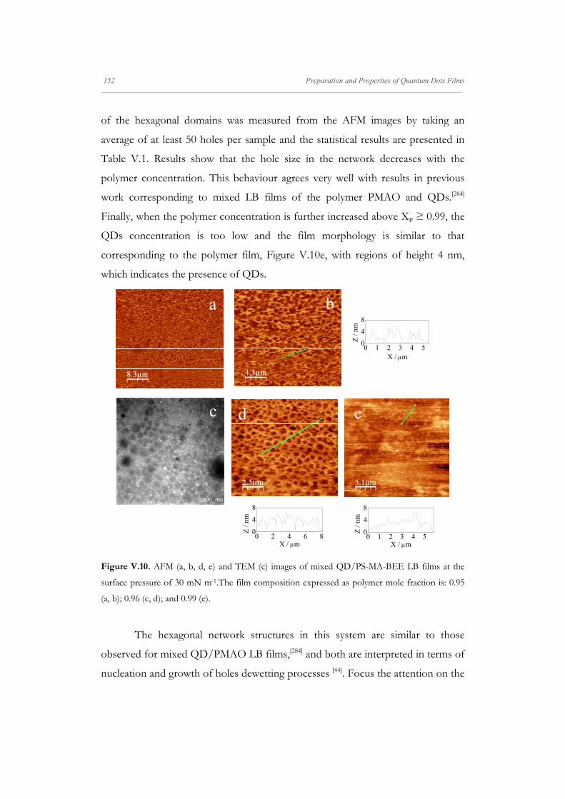
152 Preparation and Properties of Quantum Dots Films _____________________________________________________________________________________________________________________
of the hexagonal domains was measured from the AFM images by taking an
average of at least 50 holes per sample and the statistical results are presented in
Table V.1. Results show that the hole size in the network decreases with the
polymer concentration. This behaviour agrees very well with results in previous
work corresponding to mixed LB films of the polymer PMAO and QDs.[284]
Finally, when the polymer concentration is further increased above XP ≥ 0.99, the
QDs concentration is too low and the film morphology is similar to that
corresponding to the polymer film, Figure V.10e, with regions of height 4 nm,
which indicates the presence of QDs.
Figure V.10. AFM (a, b, d, e) and TEM (c) images of mixed QD/PS-MA-BEE LB films at the
surface pressure of 30 mN m-1.The film composition expressed as polymer mole fraction is: 0.95
(a, b); 0.96 (c, d); and 0.99 (e).
The hexagonal network structures in this system are similar to those
observed for mixed QD/PMAO LB films,[284] and both are interpreted in terms of
nucleation and growth of holes dewetting processes [44]. Focus the attention on the
d
0 2 4 6 80
4
8
Z /
nm
X / m
f
1000 nm
c e
0 1 2 3 4 50
4
8
Z /
nm
X / m
0 1 2 3 4 50
4
8
Z /
nmX / m
a b

Preparation and Properties of Quantum Dots Films 153 _____________________________________________________________________________________________________________________
nucleation and growth of holes, this dewetting mechanism is driven by
gravitational effects, consequently, it is easy to understand that this effect
predominates in films containing high molecular weight material such as the
polymer PMAO (40 kDa).[284] However, it is not so evident in the QD/PS-MA-
BEE films because the polymer PS-MA-BEE (2.5 kDa) is too small. To interpret
this behaviour it is necessary to analyze the balance between the driving forces
involved in the surface arrangement: gravitational and capillary forces, Figure
V.11. As was mentioned, it is well established that the damping coefficient passes
though a maximum at low elasticity values[288, 292] and decreases when the elasticity
modulus increases. Thus, according to the elasticity curves, Figure V.4c, the
elasticity goes through a minimum for QD/PS-MA-BEE monolayers at the
surface pressure value of 30 mN m-1 and for polymer concentrations above 0.95.
Consequently, in these monolayers the capillary waves are quickly damped and the
film breaks in domains separated by holes due to gravitational effects. Conversely,
the capillary waves for monolayers with higher elasticity values (π = 14 mN m-1 or
π = 30 mN m-1 and XP < 0.95), do not damp so quickly and they drive the
dewetting mechanism. In these situations, the spinodal dewetting mechanism
predominates against the growth of holes process leading to circular QDs
domains.
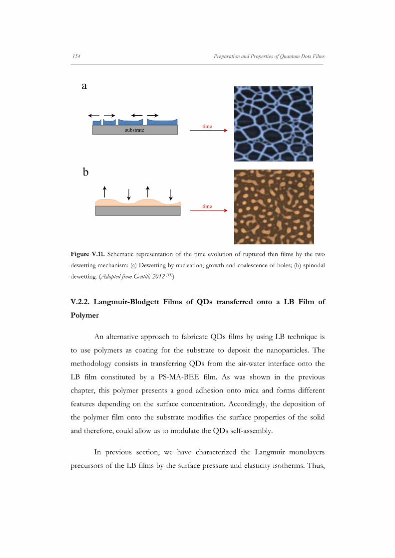
154 Preparation and Properties of Quantum Dots Films _____________________________________________________________________________________________________________________
Figure V.11. Schematic representation of the time evolution of ruptured thin films by the two
dewetting mechanism: (a) Dewetting by nucleation, growth and coalescence of holes; (b) spinodal
dewetting. (Adapted from Gentili, 2012 [44])
V.2.2. Langmuir-Blodgett Films of QDs transferred onto a LB Film of
Polymer
An alternative approach to fabricate QDs films by using LB technique is
to use polymers as coating for the substrate to deposit the nanoparticles. The
methodology consists in transferring QDs from the air-water interface onto the
LB film constituted by a PS-MA-BEE film. As was shown in the previous
chapter, this polymer presents a good adhesion onto mica and forms different
features depending on the surface concentration. Accordingly, the deposition of
the polymer film onto the substrate modifies the surface properties of the solid
and therefore, could allow us to modulate the QDs self-assembly.
In previous section, we have characterized the Langmuir monolayers
precursors of the LB films by the surface pressure and elasticity isotherms. Thus,
a
b
substratetime
time

Preparation and Properties of Quantum Dots Films 155 _____________________________________________________________________________________________________________________
we choose the polymer LB film prepared from the Langmuir monolayer at the
surface pressure of 14 mN m-1, corresponding to the maximum elasticity state,
because it is composed by wide stripes that could favour the adsorption of the
QDs. At this state, a good polymer coverage is achieved. On the other hand, the
QDs elasticity isotherm obtained from the surface pressure isotherm also shows a
maximum at the surface pressure of 9 mN m-1. Thus, this surface pressure is
chosen for the QDs LB deposition together with a higher value, 30 mN m-1, in
order to evaluate the effect of QDs concentration on the film morphology. To
compare the effect of the polymer layer, Figure V.12 present the AFM and TEM
images of the QD LB film at 9 mN m-1 and 30 mN m-1 directly deposited onto
mica.
Figure V.12. AFM (a, b) and TEM (c, d) images of QDs LB films deposited at the surface
pressures of 9 (a, c) and 30 (b, d) mN m-1.
156 Preparation and Properties of Quantum Dots Films _____________________________________________________________________________________________________________________
We transfer the QDs onto the polymer LB film at two different surface
pressure values 9 and 30 mN m-1. Figure V.13 shows the AFM and TEM images
of these LB films. The images indicate that the film is mainly constituted by QD
domains with irregular architecture. The density of domains increases when the
surface pressure of the QDs Langmuir monolayer increases, Figure V.13d.
However, the increase of the population of domains does not modify the features
of QDs and island-like QDs aggregates are also observed. It is interesting to note
that the nanoparticles are randomly adsorbed on the polymer LB film.
Consequently, the stripes observed in the polymer LB film cannot be used as
pattern for nanoparticle deposition. Besides, the AFM height profiles in Figure
V.13 indicate that no 3D aggregates are formed. Thus, by comparing with QD
films directly deposited onto mica, Figure V.12, the polymer film avoids the QD
agglomeration.

Preparation and Properties of Quantum Dots Films 157 _____________________________________________________________________________________________________________________
Figure V.13. AFM (a, c) and TEM (b, d) images of QDs LB films deposited onto a PS-MA-BEE
LB film at the surface pressures of 9 (a, b) and 30 (c, d) mN m-1. The polymer LB film was
deposited at the surface pressure of 14 mN m-1.
To understand the differences observed between the QDs assembly on
the mica and on the polymer LB film, it is necessary to analyze the driving forces
involved in the surface arrangement. In the case of bare mica, the QD
agglomeration in the films deposited is mainly due to the preferential attractions
between the nanoparticles [143] in comparison with the QD-mica attractions. This
occurs in low energy substrates such as mica (0.38 mN m-1). However, when the
substrate is covered with the polymer, the surface energy is increased minimizing
the dewetting processes.[293, 294] In this situation, the nanoparticles assembly
process can be related to the interaction between the neighbouring layers.[295]
Accordingly, we interpret our results by analyzing the ability of QDs to wet the
100 nm
0 1 20
2
4
Z /
nm
X / m
0 2 40
2
4
Z /
nm
X / m
a b
c d

158 Preparation and Properties of Quantum Dots Films _____________________________________________________________________________________________________________________
polymer coating by means of the spreading parameter. The spreading parameter
has been used previously in LB films to evaluate their stability [296] and to interpret
the nanostructures formed by nanoparticles on substrates with different natures [297]. Moreover, it is established that the ability of a thin film to wet the substrate
and form smooth films is related to the interfacial energy when there is no specific
interactions between the layers.[298] Therefore, we analyze the spreading parameter
indicative of the balance between QD-polymer (adhesive forces) and QD-QD
(cohesive forces) intermolecular forces.
The spreading parameter, S, is calculated by:
/ ⁄ ⁄ ; where γpolymer/air, γQD/polymer
and γQD/air , represent the surface tensions at the polymer-air, QDs-polymer and
QDs-air, interfaces respectively.[44] The QDs surface tension value used in these
calculations was taken from the literature as γQD/air = 33 mN m-1.[13] To determine
the γpolymer/air , we consider the surface tension value of the hydrophobic moiety
exposed to the air. In this case, taking into account that it is a Y-type LB
deposition, the polystyrene (PS) block is oriented to the air, therefore γpolymer/air can
be approximated as the polystyrene/air surface tension 39.3 mN m-1.[299] On the
other hand, since the interface for PS-MA-BEE//QDs films is constituted by
styrene groups of the polymer PS-MA-BEE and the hydrocarbon chains
corresponding to the QDs stabilizer TOPO, the γQD/PSMABEE was taken as the
interfacial tension between polystyrene and polyethylene molecules [300], 8.3 mN
m-1 [299]. By using these interfacial tension values the spreading parameter S
estimated for the PS-MA-BEE//QDs system is negative. This means that the
QDs do not spread well on the PS-MA-BEE LB film.[44] This could be
consequence of weaker interaction between the nanoparticles stabilizer, TOPO,
and the polymer PS-MA-BEE deposited on the solid as compared with the QD-
QD interactions. Accordingly, the QD-QD attractive interaction prevails against
the PS//QD interaction promoting the QDs aggregation forming islands.
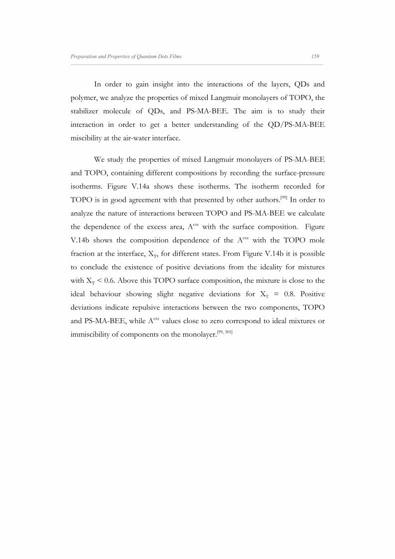
Preparation and Properties of Quantum Dots Films 159 _____________________________________________________________________________________________________________________
In order to gain insight into the interactions of the layers, QDs and
polymer, we analyze the properties of mixed Langmuir monolayers of TOPO, the
stabilizer molecule of QDs, and PS-MA-BEE. The aim is to study their
interaction in order to get a better understanding of the QD/PS-MA-BEE
miscibility at the air-water interface.
We study the properties of mixed Langmuir monolayers of PS-MA-BEE
and TOPO, containing different compositions by recording the surface-pressure
isotherms. Figure V.14a shows these isotherms. The isotherm recorded for
TOPO is in good agreement with that presented by other authors.[99] In order to
analyze the nature of interactions between TOPO and PS-MA-BEE we calculate
the dependence of the excess area, Aexc with the surface composition. Figure
V.14b shows the composition dependence of the Aexc with the TOPO mole
fraction at the interface, XT, for different states. From Figure V.14b it is possible
to conclude the existence of positive deviations from the ideality for mixtures
with XT < 0.6. Above this TOPO surface composition, the mixture is close to the
ideal behaviour showing slight negative deviations for XT = 0.8. Positive
deviations indicate repulsive interactions between the two components, TOPO
and PS-MA-BEE, while Aexc values close to zero correspond to ideal mixtures or
immiscibility of components on the monolayer.[99, 301]
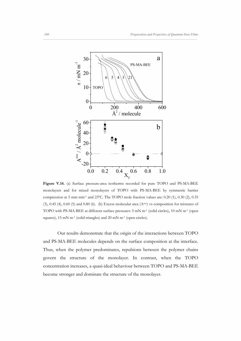
160 Preparation and Properties of Quantum Dots Films _____________________________________________________________________________________________________________________
0 200 400 6000
10
20
30
0.0 0.2 0.4 0.6 0.8 1.0-20
0
20
40
60
/ m
N m
-1
Å2 / molecule
PS-MA-BEE
TOPO
6 5 4 3 21
a
b
Aex
c / Å
2 mol
ecul
e-1
XT
Figure V.14. (a) Surface pressure-area isotherms recorded for pure TOPO and PS-MA-BEE
monolayers and for mixed monolayers of TOPO with PS-MA-BEE by symmetric barrier
compression at 5 mm min-1 and 23ºC. The TOPO mole fraction values are: 0.20 (1), 0.30 (2), 0.35
(3), 0.45 (4), 0.60 (5) and 0.80 (6). (b) Excess molecular area (Aexc) vs composition for mixtures of
TOPO with PS-MA-BEE at different surface pressures: 5 mN m-1 (solid circles), 10 mN m-1 (open
squares), 15 mN m-1 (solid triangles) and 20 mN m-1 (open circles).
Our results demonstrate that the origin of the interactions between TOPO
and PS-MA-BEE molecules depends on the surface composition at the interface.
Thus, when the polymer predominates, repulsions between the polymer chains
govern the structure of the monolayer. In contrast, when the TOPO
concentration increases, a quasi-ideal behaviour between TOPO and PS-MA-BEE
become stronger and dominate the structure of the monolayer.

Preparation and Properties of Quantum Dots Films 161 _____________________________________________________________________________________________________________________
Although it is not possible to establish a direct comparison, the results
observed in mixed monolayers of PS-MA-BEE and TOPO point to the existence
of repulsions between the QD stabilizer, TOPO, and the polymer PS-MA-BEE.
This fact can be consistent with the spreading parameter value calculated above
and the formation of QD islands in the bilayer system.
V.2.3. Surface Ligand Exchange: PSMABEE-capped QDs
Previous work demonstrated that the nature of the surface cap influences
the interactions between QDs and consequently, the properties of the
nanoparticles.[8] Therefore, to study the effect of the capping molecule on the
QDs self-assembly at the interface and to exploit the self-assembly properties of
copolymers at the air-water interface for the organization of QDs,[150] we prepare
QDs capped with the polymer PS-MA-BEE, QDP, hereafter. The surface
modification is achieved through surface ligand exchange reaction [139].
V.2.3.1. Surface Ligand Exchange Process
It has been reported that it is possible the surface ligand modification of
QDs by exchange reactions. In the case of TOPO ligand, it could be replaced by
free carboxylic (-COOH), amine (-NH2) or thiol (-SH) groups under mild
conditions such as sonication or reflux by interaction of the surface core Cd2+
with the oxygen, nitrogen or sulfur, respectively.[8] In our case, we could use the
polymer PS-MA-BEE because it has a free carboxylic group. Moreover, as the
polymer has an anhydride block, offers the possibility to open the maleic
anhydride ring by hydrolysis to form carboxylic acid groups that provides
functionality to the particles enabling the immobilization of other molecules such
as proteins on the QDs film surface.[70]

162 Preparation and Properties of Quantum Dots Films _____________________________________________________________________________________________________________________
To replace the TOPO surface ligand on the QDs by the polymer PS-MA-
BEE we use the method proposed by Xu and collaborators.[139] The method
consists in exposing the QDs stabilized by TOPO to a large excess of the
competing capping group. Thus, the TOPO-capped QDs powder was dissolved
in a PS-MA-BEE (17 mg mL-1) solution by using CHCl3/CH3OH (5:1, v/v) as
solvent and then were sonicated for 30 min, Figure V.15.
Figure V.15. Scheme of the different stages in the QDs surface ligand exchange process.
To remove the excess of ligands, TOPO and PS-MA-BEE, the solution was
precipitated with large amount of cold methanol followed by washing with
methanol and dried in vacuum. A scheme of this process is presented in Figure
V.16.
Figure V.16. Pictures of the precipitation stage in the QDs surface ligand exchange process: (a)
Beginning of the PS-MA-BEE capped-QDs precipitation with cold methanol; (b) Precipitation
after several washing steps with cold methanol; (c) QDs collected after remove the last methanol
washing by a slight centrifugation step at 1000 rpm.
In order to achieve a good removing of the free ligand excess, the PS-MA-
BEE excess and the TOPO ligands detached, we follow the washing steps by UV-
PO
PO P
OP
O
PO
PO
POP
O
P O
PO
SONICATION
Ligand Exchange in a two‐phase
polymer solution
PO
PO
PO
PO
PO
PO
PO
PO
PO
PO
PO
PO
Precipitation and washing
PS‐MA‐BEE
a b c

Preparation and Properties of Quantum Dots Films 163 _____________________________________________________________________________________________________________________
vis technique. We carry out the UV-vis spectrum of aliquots extracted of each
washing steps and continuous washing steps until the value of the absorbance
spectrum recorded is smaller enough (< 0.1 at 350 nm). Thus, more washing steps
do not allow us to remove more ligands and a stable situation is reached. This
corresponds to five or six washing steps. Finally, the PS-MA-BEE-capped QDs,
QDP, were dissolved in CHCl3/CH3OH (5:1, v/v) to prepare the spreading
solution.
FTIR was used as a probe of the efficiency of the ligand exchange process.
For the sake of comparison, Figure V.17 shows the FTIR spectra of pure TOPO
and PS-MA-BEE and PS-MA-BEE-capped nanocrystals, QDP. The FTIR
spectrum of TOPO presents a peak at 1144 cm-1 corresponding to the P=O
stretch. It was demonstrated that this peak is shifted to 1114 cm-1 upon
complexation with CdSe.[279] Therefore, the peak centred at 1124 cm-1 that appears
on the FTIR spectrum of QDP can be ascribed to the not exchanged TOPO
molecules upon the ligand exchange, bound to the nanoparticle surface. However,
the low intensity of this band indicates that a small amount of TOPO remains in
the QDP capping after the exchange process.

164 Preparation and Properties of Quantum Dots Films _____________________________________________________________________________________________________________________
2000 1800 1600 1400 1200 1000
50
100
150
1850 1800 1750 170050
60
70
80
90
TOPO
PS-MA-BEE
QDP
%T
/ a.
u.
wavenumber / cm-1
P=OStretch
CH3
Bend
%T
/ a.
u.
wavenumber / cm-1
QDP
PS-MA-BEE
Figure V.17. FTIR spectra of TOPO, PS-MA-BEE and PS-MA-BEE-capped QDs (QDP)
dispersed in KBr. The inset shows the decomposition of the carbonyl band in Gaussian functions
for pure the polymer PS-MA-BEE and for PS-MA-BEE-capped QDs. For clarity, the %T-scale is
shifted.
In addition, the appearance of the carbonyl-stretching band in the FTIR
spectrum of QDP unambiguously supports the presence of a polymer layer on the
QDs surface. For comparison we have analyzed the carbonyl band of free
polymer and polymer-capped quantum dots. The band was fitted to a sum of
three Gaussian functions centred at 1710 cm-1, 1740 cm-1 and 1782 cm-1. The
bands centred at 1710 cm-1 and 1740 cm-1 are assigned to the carbonyl stretching
of the carboxylic and ester groups, respectively and the band centred at 1782 cm-1
is assigned to the poly(maleic anhydride).[302] As can be seen in the inset of Figure
V.17 the position and the relative intensity of these bands are similar in both, the
free polymer and the PS-MA-BEE-capped QDs. All results may indicate that

Preparation and Properties of Quantum Dots Films 165 _____________________________________________________________________________________________________________________
TOPO molecules adsorbed at the QDs surface have been efficiently replaced by
the polymer PS-MA-BEE.
The nanoparticle size was calculated from the position of the maximum of
the first excitonic peak of the UV-Vis absorption spectrum, Figure V.18. The UV-
Vis spectrum of QDP in solution is blue-shifted 35 nm respect to the one
corresponding to QDs stabilized by TOPO. This fact indicates that the
replacement of TOPO by PS-MA-BEE decreases the QDs size. The diameter of
the QDP nanoparticles found was (2.8 ± 0.3) nm that corresponds to a
wavelength position of (542 ± 5) nm for the first excitonic absorption peak [204]
slightly influenced by the presence of methanol in the solution [303]. However this
size was confirmed by TEM measurements.
400 450 500 550 600 650 700
0
1
2
UV
-Vis
Abs
orba
nce
/ PL
Int
ensi
ty (
a.u.
)
/ nm Figure V.18. Absorption and emission spectra normalized of a PSMABEE-capped CdSe QDs
solution in CHCl3/CH3OH (5:1, v/v). Photoluminescence (PL) excitation at 405 nm.
V.2.3.2. Langmuir and Langmuir-Blodgett Films of PS-MA-BEE-capped
QDs
We use these modified QDP to construct the Langmuir films precursors of
the LB films. Therefore, we characterize the Langmuir monolayers by recording

166 Preparation and Properties of Quantum Dots Films _____________________________________________________________________________________________________________________
the surface pressure isotherms of pure QDP and mixtures of QDP with PS-MA-
BEE. Figure V.19a collects the isotherms obtained for different compositions and
pure QDP as inset. As can be seen in the figure the isotherms become more
condensed when the polymer concentration increases. The isotherms present a
plateau when the surface pressure reaches the value of 30 mN m-1. This behaviour
is similar to that observed for mixed monolayers containing PS-MA-BEE and
QDs stabilized with TOPO. Likewise, the equilibrium elasticity isotherms are
independent of the QDP concentration and similar to the polymer one presenting
a maximum at the surface pressure of 14 mN m-1 and a minimum at 30 mN m-1,
Figure V.19b. This fact indicates that the elasticity behaviour of these mixtures is
governed by the polymer. This behaviour was previously explained, in section
V.2.1, according to the existence of the polymer regimes: stripes and brush
conformation, respectively.

Preparation and Properties of Quantum Dots Films 167 _____________________________________________________________________________________________________________________
0.01 0.1 10
20
40
20 40 60 800
10
20
30
/ m
N m
-1
QD
/ mg m-2
/ m
N m
-1
PS-MA-BEE
/ mg m-2
PS-MA-B
EE 1 2 3 4
0 10 20 300
20
40
60
80
PS-MA-BEE
QDP
0 / m
N m
-1
/ mN m-1
Figure V.19. (a) Surface pressure isotherms of mixed monolayers of PSMABEE-capped CdSe
QDs with PS-MA-BEE with different polymer molar fraction: (0.50) (line 1), (0.96) (line 2), (0.98)
(line 3) and (0.99) (line 4). For comparison the isotherm of pure PS-MA-BEE and QDP (inset) are
represented in the figure. (b) Equilibrium surface elasticity vs. surface pressure for several mixed
Langmuir monolayers of QDP and PS-MA-BEE at different polymer mole fraction: QDP
(triangles); 0.96 (diamonds); 0.99 (starts) and PS-MA-BEE (circles). The isotherms were recorded
at 23 ºC by barrier symmetric compression at a speed of 5 mm min-1.

168 Preparation and Properties of Quantum Dots Films _____________________________________________________________________________________________________________________
The BAM images of several mixtures were taken to analyze the effect of
the polymer concentration on the morphology of the Langmuir films, Figure
V.20. As was observed for QD/PS-MA-BEE mixed monolayers, when the
polymer concentration at the air-water interface increases the QDs domains
become smaller. As in the case of TOPO-capped QDs the agglomeration is
promoted by the preferential QD-QD attractive interactions through the ligand,
PS, in contrast to the weak interaction with water subphase,[143, 153] Figure V.20a.
However, the polymer addition favours the nanoparticles spreading at the air-
water interface by its hydrophilic blocks[67, 70, 147], Figure V.20b-c.
Figure V.20. BAM images (image size 800x600 µm) of pure QDP (a) and mixed monolayers (b, c)
of the polymer PS-MA-BEE and QDP at the surface pressure of 14 mN m-1. The different
polymer mole fraction are: (b) 0.96 and (c) 0.99.
The next step was to transfer the Langmuir monolayers from the air-water
interface onto mica by LB technique. The surface pressure value of the monolayer
selected was 14 mN m-1, corresponding to the maximum elasticity states. Thus,
the results can be compared with those of mixed films of TOPO-capped QDs
and PS-MA-BEE deposited at 14 mN m-1. Figure V.21 presents AFM and TEM
images of LB films of pure QDP and mixed QDP/PS-MA-BEE. These images
show that the QDP LB films are formed by material around holes, Figure V.21a.
The height profile average value determined by AFM was 3 nm, which is
consistent with the QDP diameter ca. 2.8 nm. This fact indicates that nanoparticles
are mainly placed on the rims of holes.
a
100 μm
b
100 μm
c
100 μm

Preparation and Properties of Quantum Dots Films 169 _____________________________________________________________________________________________________________________
Figure V.21. AFM (a, c, d) and TEM (b) images of QDP and mixed QDP/ PS-MA-BEE films
deposited at the surface pressure of 14 mN m-1. The film composition expressed as polymer mole
fraction is: QDP (a, b) and 0.50 (c, d).
AFM and TEM images of mixed QDP/PS-MA-BEE LB films in Figures
V.21c-d and 22, show that the network is maintained when the polymer is added.
However, the network morphology depends on the polymer concentration. Thus,
when the polymer concentration increases the hole and rim sizes go through a
maximum at polymer mole fraction 0.5. When the polymer concentration is
further increased until XP > 0.97, AFM and TEM images show the smallest
network dimensions. TEM images magnification, Figures. V.22c and d, seem
indicate that the polymer molecules are preferentially located on rims, while the
nanoparticles are in different regions of the both rims and holes. To illustrate this
behaviour the statistical analysis of the network dimension is collected in Table
V.2. These results allow us to analyze changes on the morphology produced by
the polymer addition. Thus, when the polymer concentration increases the hole
size and the rim width decrease. In contrast, the rim height is independent of the
0 1 2 3 4 5 60
2
4
Z /
nm
X / m
c d
0.0 0.5 1.00
2
4
Z /
nm
X / m500 nm
a b
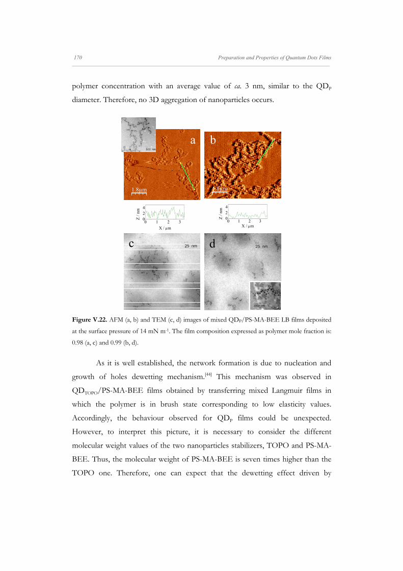
170 Preparation and Properties of Quantum Dots Films _____________________________________________________________________________________________________________________
polymer concentration with an average value of ca. 3 nm, similar to the QDP
diameter. Therefore, no 3D aggregation of nanoparticles occurs.
Figure V.22. AFM (a, b) and TEM (c, d) images of mixed QDP/PS-MA-BEE LB films deposited
at the surface pressure of 14 mN m-1. The film composition expressed as polymer mole fraction is:
0.98 (a, c) and 0.99 (b, d).
As it is well established, the network formation is due to nucleation and
growth of holes dewetting mechanism.[44] This mechanism was observed in
QDTOPO/PS-MA-BEE films obtained by transferring mixed Langmuir films in
which the polymer is in brush state corresponding to low elasticity values.
Accordingly, the behaviour observed for QDP films could be unexpected.
However, to interpret this picture, it is necessary to consider the different
molecular weight values of the two nanoparticles stabilizers, TOPO and PS-MA-
BEE. Thus, the molecular weight of PS-MA-BEE is seven times higher than the
TOPO one. Therefore, one can expect that the dewetting effect driven by
1.8µm 1.8µm
0 1 2 3024
Z /
nm
X / m
0 1 2 3024
Z /
nmX / m
a b
c d
1000 nm

Preparation and Properties of Quantum Dots Films 171 _____________________________________________________________________________________________________________________
gravitational effects, the growth of holes mechanism, prevailed over capillary
waves in nanoparticles with higher mass as QDP.
Table V.2. Average values of the feature dimensions of QDP/PS-MA-BEE mixed LB films
deposited at a surface pressure of 14 mN m-1 obtained from AFM measurements.
Hole size Rim sizeXP Diameter / μm
0.84 ± 0.34 3.61 ± 2.00
Width / μm 0.13 ± 0.13 1.21 ± 0.75
QDP
0.50 0.98 0.12 ± 0.03 0.15 ± 0.040.99 0.11 ± 0.04 0.08 ± 0.02
Reported values are averages and error represents the standard deviation determined from at least
20 surface features.
Finally, we have prepared a bilayer with QDP and PS-MA-BEE. The
methodology used is the same that in the case of nanoparticles stabilized with
TOPO. Firstly we prepared the polymer LB film transferring the PS-MA-BEE
monolayer at the surface pressure of 14 mN m-1 on mica. Then, the QDP
monolayer at the surface pressure of 14 mN m-1, was transferred onto this
polymer LB film. Figure V.23 presents the TEM and AFM images of this bilayer
system. As can be seen, the morphology of this film is different to both, the QDP
LB film, Figure V.21a, and the bilayer system prepared with TOPO-capped QDs,
Figure V.13a. By comparing with the QDP LB film, it can be concluded that the
polymer film used as coating avoids the dewetting processes observed in Figure
V.21a. On the other hand, conversely to the bilayer prepared with TOPO-capped
QDs, the PS-MA-BEE//QDP system presents a better QDs spreading leading to
a more homogeneous distribution and smaller domains. This makes sense if we
take into account that the polymer film used as template exposes the polystyrene
group and the possible distribution of the polymer capping around the
nanoparticle metal core. The polymer is bound to the surface of the CdSe crystal
by the carboxylic group, leaving the polystyrene group exposed. Consequently, the
affinity to the polymer coating is greater for the QDP than for the QDTOPO. In this
situation, γpolymer/air ~ γQD/air ~ γPS/air and γQD/polymer ~ 0. Therefore, the spreading
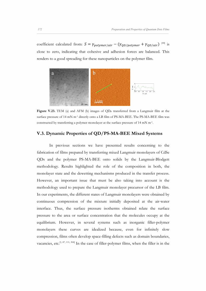
172 Preparation and Properties of Quantum Dots Films _____________________________________________________________________________________________________________________
coefficient calculated from: / ⁄ ⁄ [44] is
close to zero, indicating that cohesive and adhesion forces are balanced. This
renders to a good spreading for these nanoparticles on the polymer film.
Figure V.23. TEM (a) and AFM (b) images of QDP transferred from a Langmuir film at the
surface pressure of 14 mN m-1 directly onto a LB film of PS-MA-BEE. The PS-MA-BEE film was
constructed by transferring a polymer monolayer at the surface pressure of 14 mN m-1.
V.3. Dynamic Properties of QD/PS-MA-BEE Mixed Systems
In previous sections we have presented results concerning to the
fabrication of films prepared by transferring mixed Langmuir monolayers of CdSe
QDs and the polymer PS-MA-BEE onto solids by the Langmuir-Blodgett
methodology. Results highlighted the role of the composition in both, the
monolayer state and the dewetting mechanisms produced in the transfer process.
However, an important issue that must be also taking into account is the
methodology used to prepare the Langmuir monolayer precursor of the LB film.
In our experiments, the different states of Langmuir monolayers were obtained by
continuous compression of the mixture initially deposited at the air-water
interface. Thus, the surface pressure isotherms obtained relate the surface
pressure to the area or surface concentration that the molecules occupy at the
equilibrium. However, in several systems such as inorganic filler-polymer
monolayers these curves are idealized because, even for infinitely slow
compression, films often develop space-filling defects such as domain boundaries,
vacancies, etc.[1, 87, 111, 304] In the case of filler-polymer films, when the filler is in the
1.1µm
0.0 0.5 1.0 1.5 2.0 2.50
2
4
Z /
nm
X / m
25 nm
a b

Preparation and Properties of Quantum Dots Films 173 _____________________________________________________________________________________________________________________
order of the matrix molecular size, filler-polymer association can take place by
chains overlapping between the fillers stabilizer and polymer. Similar associations
were previously observed in polymers or nanoparticles (NPs). This kind of
association slow down the dynamics in spaces between components rending
transient metastable states that finally relax towards the minimum energy
configuration of the domain. [1, 87, 111, 304] A common strategy to achieve the stable
state is to apply successive compression-expansion cycles and then to stop the
barriers. After barriers stop, the system relaxes until it reaches a new stable state in
which the surface pressure value remains constant with time. Using this approach
more homogeneous and ordered nanoparticle (NP) monolayers can be
obtained.[18]
Accordingly, we study the surface dynamic properties in QDs and
polymer mixed films in order to improve the understanding of the hybrid system
response to mechanical stress related to the film composition and morphology. It
has been also proposed the employment of Langmuir monolayers as a platform to
analyze the dynamic properties of ultrathin films. Recent studies about NPs
dynamic behaviour have focused the investigations on the elastic and granular
character of floating pliolite particle rafts,[19] the silica NPs viscoelastic
properties[154] or as was mentioned, the induced organization of Au NPs with
shearing [18]. Moreover, mixed Langmuir monolayers were proposed to study the
modification of pulmonary surfactant interfacial properties due to the presence of
silica or carbon black NPs.[21, 155] In these studies, the authors demonstrated the
potential application of this technique to carry out nanocomposite dynamic
studies, and to best of our knowledge, showed a lack of studies for mixtures of
QDs and polymers.
In this section we analyze the effect of compression cycles on the
properties of mixed monolayers of QDs and the polymer PS-MA-BEE. The next
step was to transfer the different monolayers onto mica by LB technique to study
the morphology of the LB films after the compression cycles. On the other hand,

174 Preparation and Properties of Quantum Dots Films _____________________________________________________________________________________________________________________
the analysis of the relaxation curves obtained after the barriers stop allows us to
obtain information about the dynamic processes at the interface.
V.3.1. Effect of Shearing on Film Morphology and Monolayer
Reorganization
Previous to apply successive compression-expansion cycles it was
necessary to select the proper surface concentration. The selection criterion was
that after compression cycles the monolayers for QDs and mixtures were far from
the film collapse or far from the brush regime in the case of monolayers with
polymer concentration above XP > 0.95. Thus, the monolayers are in the same
state, concretely liquid expanded. Besides, the surface concentration should be in
the range where collective motions exist without film collapse, allowing the study
of interconnected films at high strains.[18] Using this criterion the surface
concentrations selected correspond to surface pressures values of 2.5 and 5 mN
m-1. We also analyze the effect of the surface composition on the elastic properties
of mixed monolayers before compression-expansion cycles at the surface
pressures selected, 2.5 and 5 mN m-1. The corresponding elasticity values of
polymer monolayers are higher than those of the QDs monolayers as was shown
in Figure V.4c. Taking into account that the equilibrium elasticity is related to the
system ability to store elastic energy, the behaviour observed indicates that in the
polymer monolayer the molecules are more packed and the mobility is more
limited than in the QDs monolayer. From this fact it is possible to conclude that
cohesive polymer-polymer interactions are stronger than the QD-QD ones.
Moreover, the elasticity values of mixed films are between the values
corresponding to the pure components, QDs and polymer monolayers, indicating
no synergistic effects in the mechanic properties of mixed monolayers.
Prior to the oscillatory barriers experiments, the stability of monolayers
after cycling was checked by recording the surface pressure in successive
compression-expansion cycles followed by a waiting step. An illustrative example

Preparation and Properties of Quantum Dots Films 175 _____________________________________________________________________________________________________________________
is shown in Figure V.24. Results in this figure correspond to the QDs monolayer
but a similar trend was observed for the other monolayers. In the experiment
represented in the figure, the barriers stop after the last expansion step. As can be
seen, in spite of the decrease of the surface pressure during the cycling period,
after the waiting step the system relaxes and reaches a constant surface pressure
value. On the other hand, results presented in Figure V.24 also show that the
amplitude of response decreases during the cycling period. This behaviour is
observed for high strains, U0 > 0.15, while for strain values below 0.15 the
amplitude of the response remains constant. Although, the value depends on the
mixture composition and the initial surface concentration. As example the strain
values for three different systems are collected in Table V.3.
0 5000 100000
5
10
15
20
25
5000 100000
2
4
(t)
/ m
N m
-1
time / s
(t)
/ m
N m
-1
time / s
Figure V.24. Oscillatory experiment results for a QDs monolayer combining successive
compression-expansion cycles with waiting steps. The experiment was carried out at a surface
pressure of 2.5 mN m-1, a strain amplitude of 0.35 and a frequency of 0.006 Hz. The inset shows a
zoom of the waiting stages.

176 Preparation and Properties of Quantum Dots Films _____________________________________________________________________________________________________________________
Table V.3. Strain values below which the amplitude of the system response remains constant at
the different mixture compositions and initial surface pressures.
Strain (U0)
XP Π = 2.5 mN m-1 Π = 5 mN m-1
QDs 0.16 0.160.50 0.25 0.210.98 0.18 0.15
The decrease of the surface pressure, observed during shearing, does not
occur since a certain number of cycles. Thus, the monolayer reaches a state where
the surface-pressure does not fall during the successive compression-expansion
cycles ranging from the cycle 40th to 49th, depending on the strain, monolayer
composition and surface concentration. In this way, when the strain and surface
concentration increase the total number of cycles necessary to reach a stable
situation of the surface-pressure decreases. Therefore, to reach this stable
situation, we established 50 cycles to perform the oscillatory experiments
The decrease of the surface pressure observed can be due to association
processes induced by shearing[18, 130, 305] or to monolayer dissolution in the
subphase. To settle this issue, several experiments in which 50 compression-
expansions followed by the barrier stop at the last expansion step at different
strains above 0.15 were carried out. If the cycling process induces monolayer
dissolution in the subphase, one expects that after the barriers stop the monolayer
relaxes until it reaches the new equilibrium state. These states must be different
for the distinct strains responsible for the dissolution process. Consequently, the
surface pressure after the relaxation must be different for the distinct strains
applied. Thus, the surface pressure values after the relaxation, referred as πend, for
monolayers of different composition were plotted against strains. For the sake of
clarity some results are represented in Figure V.25.

Preparation and Properties of Quantum Dots Films 177 _____________________________________________________________________________________________________________________
0.15 0.20 0.25 0.300
2
4
6
end /
mN
m-1
U0
Figure V.25. Variation of the surface pressure values reached after a waiting stage for several
monolayers at different polymer mole fraction: QDs (circles), 0.50 (squares) and 0.98 (stars), with
the strain applied in the previous oscillatory experiment. The oscillatory experiments (50 cycles)
were carried out at a frequency of 0.006 Hz and an initial surface pressure of 5 mN m-1.
As can be seen in the figure, the surface pressure value is independent of
the strain for each monolayer studied. This trend was observed for the rest of
monolayers. Accordingly, the surface pressure decrease after cycling cannot be
associated to monolayer dissolution, because even at the highest strain the
monolayer reaches a similar state to those reached with low strains. This fact can
be interpreted considering that the monolayer shearing induces aggregation
between the materials at the air-water interface, and after cycling stop, the
aggregates reach a new state. The nature of this new state seems to depend on the
film composition as revealed by the different surface pressure values achieved for
monolayers of the distinct composition.
All these experimental results point to complex dynamic processes at the
interface. Therefore, to gain insight into the dynamics of monolayers, the
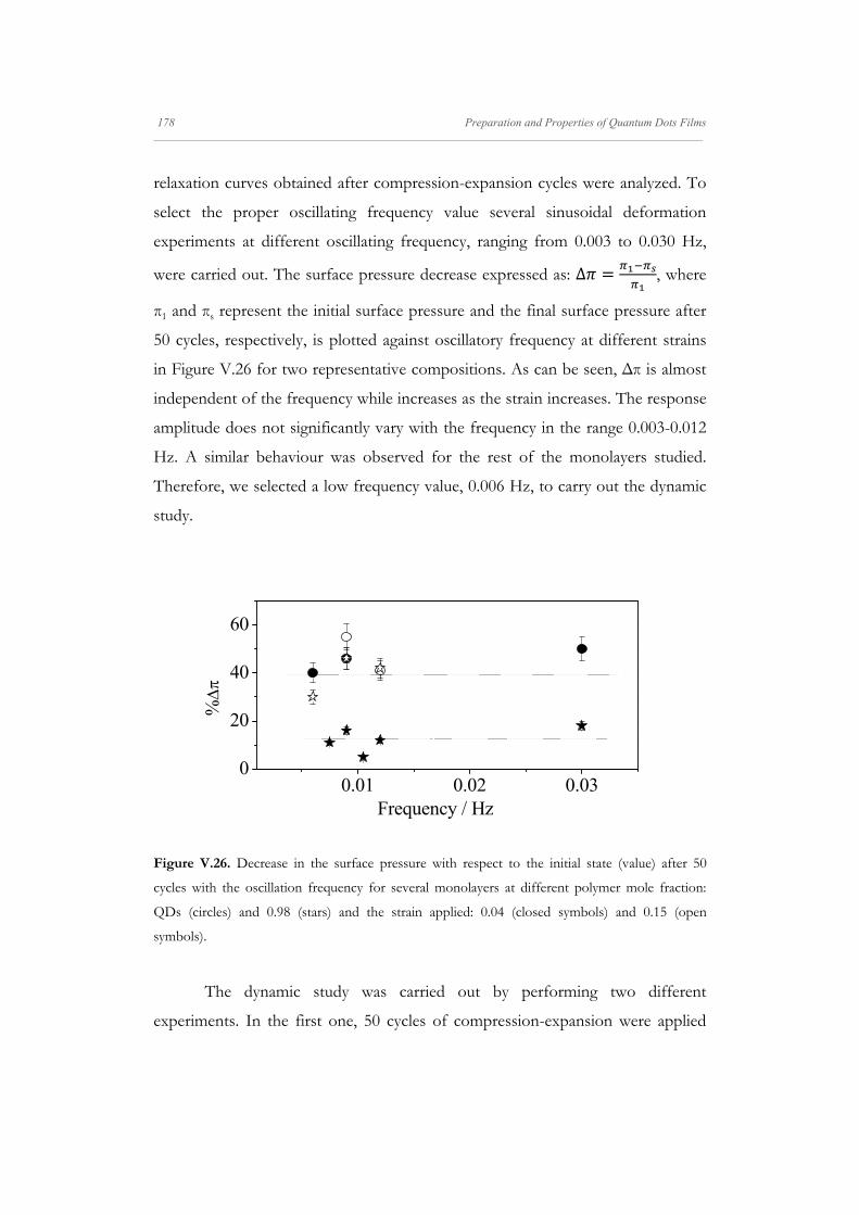
178 Preparation and Properties of Quantum Dots Films _____________________________________________________________________________________________________________________
relaxation curves obtained after compression-expansion cycles were analyzed. To
select the proper oscillating frequency value several sinusoidal deformation
experiments at different oscillating frequency, ranging from 0.003 to 0.030 Hz,
were carried out. The surface pressure decrease expressed as: ∆ , where
π1 and πs represent the initial surface pressure and the final surface pressure after
50 cycles, respectively, is plotted against oscillatory frequency at different strains
in Figure V.26 for two representative compositions. As can be seen, Δπ is almost
independent of the frequency while increases as the strain increases. The response
amplitude does not significantly vary with the frequency in the range 0.003-0.012
Hz. A similar behaviour was observed for the rest of the monolayers studied.
Therefore, we selected a low frequency value, 0.006 Hz, to carry out the dynamic
study.
0.01 0.02 0.030
20
40
60
%
Frequency / Hz
Figure V.26. Decrease in the surface pressure with respect to the initial state (value) after 50
cycles with the oscillation frequency for several monolayers at different polymer mole fraction:
QDs (circles) and 0.98 (stars) and the strain applied: 0.04 (closed symbols) and 0.15 (open
symbols).
The dynamic study was carried out by performing two different
experiments. In the first one, 50 cycles of compression-expansion were applied

Preparation and Properties of Quantum Dots Films 179 _____________________________________________________________________________________________________________________
and the barriers were stopped at the end of the last compression. In the second
experiment, after 50 cycles the barriers were stopped at the end of the last
expansion. Then, the surface pressure was recorded with time until it reaches a
constant value. We establish that the new equilibrium state is reached when the
surface pressure is constant along the time. Figure V.27 presents representative
relaxation curves for the different monolayers. The curves do not follow the
exponential law and can be interpreted as a sum of three exponential functions for
all systems except for polymer relaxation. In the later, the curves are interpreted
by a sum of two exponential functions. Lines in the examples shown in Figure
V.27 are calculated with the sum of three exponentials and the relaxation time
values obtained in the fit procedure. Results in Figure V.27 represent an
illustrative example of two experiments stopped at the end of the last
compression for a QD/PS-MA-BEE mixed monolayer (XP = 0.98), Figure V.27a
and the last expansion for a QD monolayer, Figure V.27b. For clarity to observe
the continuous cycles in Figure V. 27, the horizontal axes of the insets are in
logarithmic scale and begin at 1000 s. Similar trends were observed for the rest of
experiments.

180 Preparation and Properties of Quantum Dots Films _____________________________________________________________________________________________________________________
0.1 1 10 100 1000 10000
0.0
0.5
1.0
1000 10000
4
6
8
((t
) - f)/
0
time / s
a
(t)
/ m
N m
-1
time / s
0.1 1 10 100 1000 10000
0.0
0.5
1.0
1000 10000
5
10
15
(t
) - 0)
/ 0
time / s
b
(t)
/ m
N m
-1
time / s
Figure V.27. A multi-exponential fit example of a QD/PS-MA-BEE mixed monolayer (XP =
0.98) relaxation after 50 cycles at the end of the last compression position at a strain of 0.06 (a). A
multi-exponential fit example of a QDs relaxation after 50 cycles at the end of the last expansion
position (strain 0.18) (b). Both, monolayers were prepared at a surface pressure of 5 mN m-1 and
oscillation experiments were carried out a frequency of 0.006 Hz.

Preparation and Properties of Quantum Dots Films 181 _____________________________________________________________________________________________________________________
The results fitting suggests at least three mechanisms that dominate the
relaxation process for QDs and QD/polymer monolayers and two relaxation
mechanisms for the polymer monolayer. The first process corresponds to
damping of surface fluctuation originated for the inertia of barriers sudden-stop
and has been observed by other authors in silica nanoparticle films [305]. This time
is the same for all systems at the different strains, U0, and has a value (time-scale)
of 20 ± 2 s. The second relaxation time, 2, is represented in Figure V.28 against
the strain for several systems prepared at different polymer mole fractions, XP,
and the values ranged from 200 to 400 s. This relaxation process was observed in
monolayers containing QDs and was not found in polymer monolayers. This
relaxation time can be related to rafts movements whose time-scale is about
several hundred seconds.[305, 306] The rafts formation can be promoted by
compression and could be responsible for the decrease of the surface pressure
observed after compression. Finally, the slowest process presents relaxation times
of several thousands of seconds and can be related to particle/polymer
movements inside the rafts.[305] The same behaviour was observed for relaxation
curves obtained when the cycling is stopped at the last expansion step, see Figure
V.28.

182 Preparation and Properties of Quantum Dots Films _____________________________________________________________________________________________________________________
200
300
400
0.0 0.1 0.2 0.3
2000
4000
6000
0.0 0.1 0.2 0.3
2000
4000
6000
200
300
400
0.0 0.1 0.2 0.3
2000
4000
6000
200
300
400
0.1 0.2 0.3
2000
4000
6000
2 / s
b
3 / s
U0
d
/ s
U0
2 / s
c
3 / s
U0
2 /
sa
3 / s
U0
Figure V.28. Relaxation times values vs. strain obtained from the multi-exponential fit of the
relaxation curves obtained for QDs and mixed QD/PS-MA-BEE monolayers, prepared at an
initial surface pressure of 5 mN m-1, after shearing 50 cycles at a frequency of 0.006 Hz stopping
the barriers at the end of the last compression (closed symbols) and expansion (open symbols)
stages. The composition of the monolayers expressed as polymer mole fraction is: QDs (a); 0.50
(b); 0.98 (c) and PS-MA-BEE (d).
It is interesting to notice that the relaxation time values are independent of
the strain, within experimental uncertainty, while depend on the monolayer
composition. In order to observe this dependence, we have calculated the average
relaxation time for each relaxation process, i , as the average of the relaxation

Preparation and Properties of Quantum Dots Films 183 _____________________________________________________________________________________________________________________
times calculated from curves obtained using different strains in each system. The
calculated values are plotted against the polymer mole fraction, XP, in Figure V.29.
For comparative purposes the relaxation times values obtained when the cycles
are stopped at the end of the expansion step are also included in the figure. As
can be seen in Figure V.29, the relaxation time found when cycles are stopped at
the end of the last compression and expansion steps agree with each others. This
fact indicates that the same processes are observed in the two experiments. The
relaxation time values ascribed to rafts movements, 2, indicate that the raft
movement becomes slightly slower when the polymer concentration increases. A
more significant dependence on composition is observed for the relaxation times,
3, corresponding to movements inside rafts and that can be related to
impediments due to the polymeric matrix. These motion impediments have been
proposed by theoretical models in nanoparticle/polymer mixtures, which are
based on the reduction of polymer mobility close to the nanoparticle surface that
promotes a local reorganization more structured. This behaviour is more marked
when the nanoparticle size is similar to the polymer chains since an enormous
interfacial area is involved.[22, 23, 307, 308] This could be in agreement with the increase
in the relaxation time observed for mixed films of the highest polymer
composition, XP=0.98, comparing to polymer monolayer , Figure V.29.
0.0 0.2 0.4 0.6 0.8 1.0
200
300
0.0 0.2 0.4 0.6 0.8 1.0
2000
3000
4000
5000
2 / s
XP
a
3 / s
XP
b
Figure V.29. Average relaxation times values vs. monolayer composition expressed as polymer
mole fraction, XP, obtained from the statistical treatment of the relaxation times obtained for QDs
and mixed QD/PS-MA-BEE monolayers, prepared at an initial surface pressure of 5 mN m-1,

184 Preparation and Properties of Quantum Dots Films_____________________________________________________________________________________________________________________
after shearing 50 cycles at a frequency of 0.006 Hz stopping the barriers at the end of the last
compression (closed symbols) and expansion (open symbols) stages.
According to the scenario proposed, a schematic model showing the two
processes involved in the nanoparticles monolayers is presented in Figure V.30.
Figure V.30. The cartoon model represents the movements that dominate the relaxation of the
monolayers that contains nanoparticles.
In an attempt to visualize the rafts movements, BAM images of the
monolayers before and after cycling were taken. Illustrative images corresponding
to the Langmuir monolayer prepared with QDs, and mixtures of QDs with PS-
MA-BEE at polymer mole fraction values of XP = 0.5 and 0.98, are collected in
Figure V.31.
Internalrearrangements
τ2
τ3
Rafts reorganization

Preparation and Properties of Quantum Dots Films 185 _____________________________________________________________________________________________________________________
Figure V.31. BAM images (800x600 μm) at the initial state of the monolayer, π = 2.5 mN m-1, (a,
b, c) and after shearing 50 cycles at high strains (U0 > 0.20) at the compression (d, e, f) and
expansion (g, h, i) stages for different QD/PS-MA-BEE monolayers with a polymer mole fraction:
QDs (a, d, g); 0.50 (b, e, h) and 0.98 (c, f, i).
BAM images of the pure polymer film show no contrast enough to
observe the monolayer morphology; consequently, we do not show images of this
film. The BAM images show that for films prepared with QDs, Figures V.31d and
g, and mixtures of polymer composition XP = 0.50, Figures V.31e and h, the
compression induces compact domains and after expansion step the film presents
cracks that propagate in the perpendicular direction to the applied stress. Mixed
films of polymer mole fraction 0.98 present domains less compacted and
consequently, the cracks produced after the expansions are greater than those
observed for other compositions.
100 μm 100 μm 100 μm
100 μm100 μm100 μm
a b c
g h i
100 μm100 μm100 μm d e f

186 Preparation and Properties of Quantum Dots Films _____________________________________________________________________________________________________________________
To confirm the raft movements, BAM images of monolayers after and
before compression are presented in Figure V.32. Arrows in the figure point to a
given raft to better visualize the raft movements. As can be clearly seen, in the
compression step the monolayers become more compact and some cracks
disappear. Conversely, the expansion step regenerates some cracks and the
monolayer becomes more expanded. The BAM images allow us to confirm rafts
movements during the shearing process. These movements present relaxation
times in the order of several hundred seconds determined from the relaxation
curves obtained after the cycling period.
Figure V.32. BAM images (800x600 μm) showing several rafts movements promoted in the
expansion stage (b, d, f) for different QD/PS-MA-BEE monolayers with a polymer mole fraction:
QDs (a, b); 0.50 (c, d) and 0.98 (e, f).
100 μm
a b
c d
e f
Preparation and Properties of Quantum Dots Films 187 _____________________________________________________________________________________________________________________
We are interested in analyzing the effect of compression cycles on the
morphology of the LB films by transferring the films after shearing 50 cycles at
low (U0=0.05) and high (U0=0.25) strain values at the end of the last compression
step. Figure V.33 shows the AFM images of different films. It is interesting to
notice that even the LB films containing small concentration of QDs (XP= 0.98),
Figures V.33e and f, present a film morphology quite different to that of the
polymer film, Figures V.33g and h. This fact indicates that QDs modify the
interactions between polymer molecules resulting in films with different
morphologies as a function of the QDs composition.[308] The AFM images also
confirm that the LB film becomes more close-packed after shearing. This fact is
more marked at high strains. For comparison, results in Table V.4 shows a
statistic study of the domain dimensions for the QD/PS-MA-BEE film at XP =
0.98 at low (0.05) and high (0.25) strains.
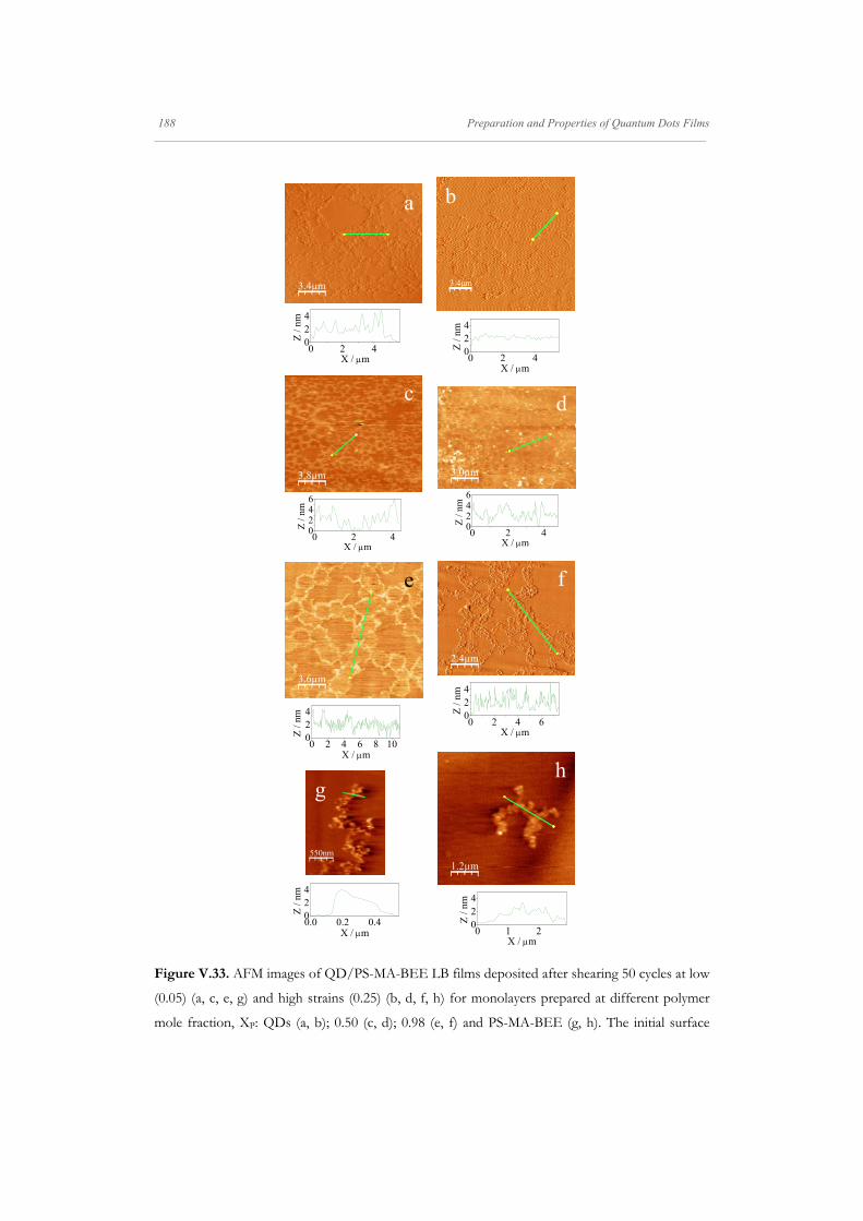
188 Preparation and Properties of Quantum Dots Films _____________________________________________________________________________________________________________________
Figure V.33. AFM images of QD/PS-MA-BEE LB films deposited after shearing 50 cycles at low
(0.05) (a, c, e, g) and high strains (0.25) (b, d, f, h) for monolayers prepared at different polymer
mole fraction, XP: QDs (a, b); 0.50 (c, d); 0.98 (e, f) and PS-MA-BEE (g, h). The initial surface
3.8µm
0 2 40246
Z /
nm
X / m
3.4µm
0 2 4024
Z /
nm
X / m
3.4µm
0 2 4024
Z /
nm
X / m
3.0µm
0 2 40246
Z /
nm
X / m
0 2 4 6 8 10024
Z /
nm
X / m
3.6µm
2.4µm
0 2 4 6024
Z /
nm
X / m
1.2µm
0 1 2024
Z /
nm
X / m
550nm
0.0 0.2 0.4024
Z /
nm
X / m
a b
c d
e f
gh

Preparation and Properties of Quantum Dots Films 189 _____________________________________________________________________________________________________________________
pressure of the monolayers was 2.5 mN m-1, except for PS-MA-BEE monolayers that was 3.5 mN
m-1.
Table V.4. Mean features dimensions of QD/PS-MA-BEE mixed LB film prepared at XP = 0.98
based on AFM measurements.
Strain (U0) X-direction / μm Y-direction / μm
0.05 2.53 ± 0.56 2.17 ± 0.270.25 0.45 ± 0.12 0.38 ± 0.13
*Reported values are averages and error represents the standard deviation determined from at least
20 surface features.
The morphology of these films was analyzed by TEM. This technique
complements the AFM images because QDs can be observed in the TEM images.
Representative TEM images of films prepared by transferring Langmuir
monolayers after 50 compression-expansion cycles are collected in Figure V.34.
TEM images of QDs, Figs. V.34a and b, correspond to aggregates obtained by
using different strains. The images show that the domain size decreases when the
strain increases. This behaviour agrees with the information obtained from the
AFM images of these films. This picture is also consistent with a directional-stress
order in the film induced by X-deformation. This behaviour was previously
observed in monolayers containing BaCrO4 nanorods.[309] TEM images for the
mixed QD/polymer films indicate that, as expected, the QDs domain size also
decreases when the QDs concentration decreases. Figures V.34c and d show that
the LB films of Xp = 0.50 presents the closest domains. The images also
demonstrate that in this film when the strain increases the domains merge in big
domains, Figure V.34d. When the polymer mole fraction is further increased until
0.98 the polymer molecules predominate and the QDs domains become smaller
than the ones observed for film with high QDs concentration, Figure V.34e and f.

190 Preparation and Properties of Quantum Dots Films _____________________________________________________________________________________________________________________
Figure V.34. TEM images of QD/PS-MA-BEE LB films deposited after shearing 50 cycles at
low (0.05) (a, c, e) and high (0.25) (b, d, f) strain for monolayers prepared at a polymer mole
fraction: (a, b) QDs; (c, d) 0.50 and (e, f) 0.98. The initial surface pressure of the monolayers was
2.5 mN m-1.
In summary, the results are in excellent agreement with those observed by
other authors who observed that the inorganic filler monolayers develop
metastable filler aggregates probably due to chains overlapping of the fillers
stabilizer.[18, 304] In the current work, we apply successive compression-expansion
cycles [18] to prepare ordered QDs monolayers. The methodology used allows us
to obtain information of the different relaxation processes produced after the
compression-expansion cycles. Thus, two relaxation processes were observed for
100 nm
1000 nm
1000 nm
1000 nm
1000 nm
1000 nm
1000 nm
a b
c
e
d
f

Preparation and Properties of Quantum Dots Films 191 _____________________________________________________________________________________________________________________
QDs and mixed QD/polymer films. The fastest one was ascribed to rafts
movements, while the slowest was related to movements inside rafts. Moreover,
the time-scales of these processes are related to the film composition. Thus,
slower relaxations correspond to systems with high polymer mole fraction.
V.4. Photoluminescence of QDs in Langmuir-Blodgett Films
In previous sections we presented different methodologies to construct
CdSe QDs films: co-spreading and bilayer approaches. Our results showed that
the morphology of these films depends on the methodology employed to prepare
them. In this section the aim is to study the effect of the film morphology on the
photoluminescence properties since the understanding of the optical properties of
assembled QDs is important for their applications. This is an important issue for
the construction of optoelectronic devices, such as LEDs, photodetectors, solar
cells and nanosensors,[9, 310, 311] where highly-ordered structures with homogeneous
and known photophysical properties[7] are necessary. In this sense, it is important
to study the influence of the QDs’ density, environment (capping and mixed
systems), inter-dot distance and excitation energy in the photophysical properties
of QDs films. Within the different spectroscopic techniques, time-resolved
photoluminescence has the advantage of being a technique highly sensitive to
surface and environmental changes, but this information is often concealed by the
intrinsically complex excited-state dynamics of QDs.[25] Therefore, the
photoluminescence dynamics of QD/PS-MA-BEE films were measured by
confocal fluorescence lifetime microscopy by analyzing the decay curves and
fluorescence images. This technique is not available at the Universidad de
Salamanca, therefore this part of the work was performed during a short stay in
the Molecular Photochemistry Group (IST, Lisbon). The results show the
influence of the different self-assembly strategies with the polymer on the
fluorescence dynamics of QDs.
192 Preparation and Properties of Quantum Dots Films _____________________________________________________________________________________________________________________
Some optoelectronic applications take advantage of QDs properties
incorporating them into a polymeric matrix building nanocomposites. In these
cases, it is necessary to develop a controlled way to achieve good-quality polymer-
QDs hybrid films.[8, 311] In order to optimize these hybrid systems, several authors
have focused their attention on the effect of film matrix properties on the energy
transfer processes [312, 313] or the QDs photoluminescence intermittency (blinking
statistics)[314, 315].
On the other hand, it is also essential to understand and modulate the
energy transfer in a QD film. Some reports indicate that in monodispersed QD
layers there is an energy transfer (ET) not only between neighbour QDs but QDs
at longer distances also contribute.[316-318] This energy transfer is due to an overlap
of the first absorption peak with the PL emission of the QDs and is faster in non-
shell QDs capped with relatively short ligand molecules, (because of the r-6
distance dependence of the energy transfer). Two non-radiative mechanisms for
energy transfer between QDs have been proposed, the Dexter exchange
mechanism and the Förster resonant energy transfer (FRET) mechanism.
However, previous theoretical and experimental studies show that energy transfer
between nanocrystal QDs can be appropriately described by FRET theory in two
dimensions proposed to biological membranes.[317]
The photoluminescence (PL) decay dynamics of colloidal QD ensembles
present long lifetimes (tens of nanoseconds at room temperature to microseconds
at low temperature) and complex behaviour reflected on multi-exponential
fluorescence decays. Several explanations have been proposed to interpret the
multi-exponential behaviour [319] in the QD ensemble PL decay dynamics: (i) each
member of the ensemble has its own unique single-exponential (single-rate)
lifetime, (ii) the PL decay is an inherently complex process for each individual
QD, making the decay dynamics multi-exponential for each member of the
ensemble, or (iii) the PL decay of each member is single exponential at any given

Preparation and Properties of Quantum Dots Films 193 _____________________________________________________________________________________________________________________
moment but it fluctuates in time, so that the time-averaged PL decay of an
individual QD is multi-exponential. Alternative explanations invoke the role of
surface defects of the nanocrystal as charge trapping sites that give rise to charge-
trapped states that lie within the band gap. Usually these charged states are non-
emissive or emit in the infrared, which further complicates the emission dynamics.
Thus, fluctuations in the local electrostatic environment surrounding the QD can
play an important role. This behaviour was studied in QD clusters by Van Orden
and co-workers[320] that have shown that QDs clusters exhibit a behaviour not
observed in isolated QDs. The QDs clusters present an enhanced blinking and a
biexponential decay characterized by a prominent fast component and a slow
component characteristic of isolated QDs. Moreover, in solid films, the PL
complexity is further increased by the possibility of excitation energy transfer
between QDs, due to the short interparticle distances in close-packed films.
V.4.1. Experimental Details
The samples were prepared by the Langmuir-Blodgett technique
transferring QDs Langmuir monolayers at different surface pressures. Atomic
Force Microscopy and Transmission Electron Microscopy were used to analyze
the morphology of the films deposited onto quartz discs and Formvar®-carbon
coated copper grids, respectively. This study was necessary because we had to
change the mica substrate by quartz discs due to mica presents an important
fluorescence emission that interferes with the QDs photoluminescence. In this
sense, prior to the PL measurements, we check the quartz substrate cleaning and
the PS-MA-BEE contributions by FLIM measurements. The visualization in both
cases of images with only dark counts indicates that the RCA clean method used
for the quartz substrates is good for FLIM characterization and the polymer
purity meets the FLIM requirements, not interfering in the measurements at the
excitation wavelength selected, 482 nm.
194 Preparation and Properties of Quantum Dots Films _____________________________________________________________________________________________________________________
The photoluminescence properties of QDs are strongly dependent on the
presence of surface defects due to the large relation surface area-volume. Thus, in
order to avoid spurious effects from QD handling that could induce different
surface conditions of QDs,[321-324] we have established a protocol of preparation of
QDs solutions and films. One single batch of synthesized QDs was used for all
the experiments. All the QD powder necessary to prepare the spreading solutions
was extracted in a single purification. The QD concentration in the spreading
solutions was the same for all samples, ca. 10-6M (0.968 µM). The solutions were
freshly prepared just before the monolayer deposition. The LB films were dried
during 12 h and stored under vacuum. To ensure no aging effects, the waiting
time between LB films preparation and FLIM measurements was the same for all
samples.
The steady-state spectroscopy was carried out in a Perkin-Elmer Lambda
35 UV-vis spectrophotometer and in a Horiba Jobin Yvon IBH FluoroLog-3
spectrofluorimeter using front-face detection with an angle of 22.5º. The emission
spectra are the average of at least ten measurements. The light dispersed by the
films deposited onto quartz substrates was corrected by subtracting the
corresponding reference sample in the absorption spectra. For fluorescence
steady-state measurements the corrected spectra were obtained using the
correction file provided with the instrument. All the spectra were recorded at
room-temperature.
For the photoluminescence studies we employed the Fluorescence
Lifetime Imaging technique using a MicroTime200 time-resolved confocal
fluorescence microscope system from PicoQuant GmbH (Berlin, Germany).
Point and area measurements (80x80 µm2, 400x400 pixels, integration time of 1ms
per pixel) were carried out by using 482 nm excitation wavelength (2.5 MHz
repetition rate, 152 ps/channel resolution, objective x60 N.A. 1.2 of water
immersion) with a band-pass 550-690 nm filter to select emission. A pinhole of
Preparation and Properties of Quantum Dots Films 195 _____________________________________________________________________________________________________________________
30 μm was used to reject out-of-focus light. The emitted light is detected with a
single-photon counting avalanche photodiode (Perkin-Elmer) and digitized by
TimeHarp 200 TD-SPC PC board (PicoQuant GmbH). To preserve LB films
from water, we used a glass coverslip between the water drop and the sample. The
measurements in solution were carried out with a quartz cuvette sample holder
and an objective x40 N.A. 0.65 in air.
V.4.2. Selection of the Experimental Conditions by Steady-state
Measurements
We carried out a series of preliminary experiments to select adequate work
conditions. The wavelength laser excitation conditions were selected taking into
account the steady-state fluorescence results of QDs in chloroform solution and
on quartz substrates. To avoid the polymer excitation, the wavelength selected
was 482 nm. At this wavelength only the QDs are excited, not the polymer
keeping away from further complications in emission behaviour [325]. When mixed
QD/PS-MA-BEE films are excited at short wavelengths, e.g. 350 nm, it is
possible to observe the bands associated to each compound, Figure V.35. The
first band centred at ~425 nm corresponds to the polymer excimer emission [326]
characteristic of polystyrene copolymers thin films [327]. The second one
corresponds to the QDs emission. Although the QD concentration varies, the
individual position of the peaks and the intensity of the polymer peak are kept
indicating that no energy transfer is expected between the QD and polymer.

196 Preparation and Properties of Quantum Dots Films _____________________________________________________________________________________________________________________
400 450 500 550 6000
1
2
3
4
5
PL I
nten
sity
(a.
u.)
/ nm
Figure V.35. PL spectrum of a QD/PS-MA-BEE mixed LB film deposited at 30 mN m-1 and
prepared with a polymer mole fraction of 0.50. The excitation wavelength was 350 nm.
For the sake of comparison, the absorption and fluorescence spectra of
QD in solution and LB deposited onto quartz were recorded in Figure V.36. A
slight shift in the fluorescence spectra can be observed. This fact could be
attributed to dipole-dipole interactions between nearest neighbour QDs, i.e., an
energy transfer.[328]
400 500 600 7000
1
2
Abs
orba
nce
/ PL
Int
ensi
ty (
a.u.
)
/ nm
Figure V.36. Absorption and PL spectra for QD in chloroform solution (red line) and a QD LB
film deposited at 30 mN m-1 (black line).
Due to we study mixed films of QDs and PS-MA-BEE, we analyze the
effect of the presence of the polymer on the QDs fluorescence emission. Figure
V.37 shows the photoluminescence (PL) spectra of different QD/polymer

Preparation and Properties of Quantum Dots Films 197 _____________________________________________________________________________________________________________________
solutions by varying the polymer mole fraction, XP. Results show a possible
quenching from the polymer due to aromatic rings could be effective quenchers
of CdSe QDs emission, i.e., be capable of directly intercepting one of the charge
carriers disrupting the radiative recombination process,[329] as shown in Figure
V.37. However, this effect is only observed at high polymer concentrations, above
XP > 0.80.
500 600 7000
10
20
400 500 600 7000.0
0.1
0.2
0.3
PL
Int
ensi
ty (
a.u.
)
/ nm
IncreasingPS-MA-BEE
Abs
orba
nce
(a.u
.)
/ nm
Figure V.37. Absorption and PL spectra of mixed QD/PS-MA-BEE chloroform solutions at
different polymer molar ratios: QDs (black); (0.50) (dark gray); (0.96) (gray) and (0.98) (light gray).
The QDs concentration is the same for all solution as indicate the absorption spectra (inset) and is
ca. 10-6 M.
In summary, the steady-state measurements allow us to determine several
work conditions: the excitation wavelength, 482 nm, and the polymer mole
fraction, XP<0.90 in order to avoid the polymer influence on the QDs
photoluminescence dynamics study.
V.4.3. Photoluminescence Dynamics of QDs
As was previously commented the PL dynamics of QDs are complex and
can be affected by several experimental conditions. In the dynamic studies of
QDs, we can observe the effect of the QDs’ density, environment (polymer),
power excitation energy and exposure time on the fluorescence average lifetime
values for the different samples obtained from multi-exponential decay fit. The

198 Preparation and Properties of Quantum Dots Films _____________________________________________________________________________________________________________________
average lifetime values allow us to compare our results with the literature.
Therefore, a preliminary analysis of these variables on the PL dynamics becomes
necessary to establish adequate work conditions to a PL dynamic study in deep of
QDs LB films.
V.4.3.1. Photoluminescence Dynamics of QDs in Solution
Since the QD-polymer hybrid films are a complex system, we began to
study the mixtures in chloroform solution. However, differences between the
distinct systems are not visible in solution, the fluorescence lifetimes are similar
and around 35 ± 2 ns, close to the value for individual QDs, see Figure V.38 and
Table V.5. Besides, the average lifetime values are not dependent on power
excitation: 35 ± 2 ns (67 W cm-2); 35 ± 2 ns (134 W cm-2) and 35 ± 1 ns (244 W
cm-2). Thus, as the polymer addition has not a dramatic effect on the average
lifetimes and the first excitonic peak (absorption spectrum Figure V.37) of QDs,
the quenching observed in the PL spectra could be attributed to an excited-state
charge-transfer mechanism.[325, 330] In this type of mechanism a high polymer
concentration, XP > 0.80, causes a decrease in the PL emission intensity, as in
Figure V.37, but the lifetimes are not strongly influenced, Table V.5. Furthermore,
the PL decay curves below this polymer mole fraction agree with the QDs one,
Figure V.38. The proximity of polymer molecules to QDs allows that the polymer
acts as hole acceptor to several hole trapping emitting sites of the QDs surface,
eliminating fluorescence sites.[331, 332]
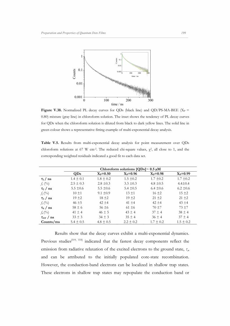
Preparation and Properties of Quantum Dots Films 199 _____________________________________________________________________________________________________________________
0 100 200 3001E-3
0.01
0.1
1
0 100 200 3001E-3
0.01
0.1
1
Cou
nts
time / ns
0.001
Cou
nts
time / ns
0.001
Figure V.38. Normalized PL decay curves for QDs (black line) and QD/PS-MA-BEE (XP =
0.80) mixture (gray line) in chloroform solution. The inset shows the tendency of PL decay curves
for QDs when the chloroform solution is diluted from black to dark yellow lines. The solid line in
green colour shows a representative fitting example of multi-exponential decay analysis.
Table V.5. Results from multi-exponential decay analysis for point measurement over QDs
chloroform solutions at 67 W cm-2. The reduced chi-square values, χ2, all close to 1, and the
corresponding weighted residuals indicated a good fit to each data set.
Chloroform solutions [QDs]~ 0.5 µMQDs XP=0.50 XP=0.96 XP=0.98 XP=0.99
τ1 / ns 1.4 ± 0.1 1.8 ± 0.2 1.5 ±0.2 1.7 ±0.2 1.7 ±0.2 f1 (%) 2.5 ± 0.3 2.8 ±0.3 3.3 ±0.3 4.8 ±0.5 4.4±0.4 τ2 / ns 5.5 ±0.6 5.5 ±0.6 5.4 ±0.5 6.4 ±0.6 6.2 ±0.6 f2 (%) 10 ±1 9.1 ±0.9 13 ±1 16 ±2 15 ±2 τ3 / ns 19 ±2 18 ±2 19 ±2 21 ±2 21 ±2 f3 (%) 46 ±5 42 ±4 41 ±4 42 ±4 43 ±4 τ4 / ns 58 ± 6 56 ±6 61 ±6 70 ±7 73 ±7 f4 (%) 41 ± 4 46 ± 5 43 ± 4 37 ± 4 38 ± 4 τAV / ns 33 ± 3 34 ± 3 35 ± 4 36 ± 4 37 ± 4 Counts/ms 5.4 ± 0.5 4.8 ± 0.5 2.2 ± 0.2 1.7 ± 0.2 1.5 ± 0.2
Results show that the decay curves exhibit a multi-exponential dynamics.
Previous studies[319, 333] indicated that the fastest decay components reflect the
emission from radiative relaxation of the excited electrons to the ground state, τr,
and can be attributed to the initially populated core-state recombination.
However, the conduction-band electrons can be localized in shallow trap states.
These electrons in shallow trap states may repopulate the conduction band or

200 Preparation and Properties of Quantum Dots Films _____________________________________________________________________________________________________________________
thermalize into deeper trap states, contributing to non-radiative relaxation
pathways. The longest lifetime components in the decay curve are attributed to
radiative recombination of carriers because they account for more and more of
the total luminescence when the quantum yield of the QDs is increased.[334]
Moreover, a distribution in decay times is expected as a result of the variation in
the non-radiative decay rates for different QDs due to a variation in type and
number of the quenching centres. A combination of all of these processes, along
with differences in shape and size between the individual nanocrystals in a
population, gives rise to multi-exponential emission dynamics.
If we compare the decay curves and components in solution vs. a LB film
of QDs, noteworthy differences are visible, see Figure V.39. The initial part of the
decay appears longer in solution where is less likely that energy transfer occurs
because of the low concentration (~ 10-6 M) and due to it is a system more fluid
than the film. On the other hand, the enhanced close-packed and rigid LB films
allow for the interactions between neighbour QDs as it is reflected in a faster
initial decay and also a longer decay tail.[316]
0 100 200 3001E-3
0.01
0.1
1
Cou
nts
time / ns
0.001
Figure V.39. Normalized PL decay curves for QDs in chloroform solution at 10-6 M (red line)
and a QDs LB film at high concentration (π = 30 mN m-1) onto quartz substrate (black line).

Preparation and Properties of Quantum Dots Films 201 _____________________________________________________________________________________________________________________
Moreover, the sharp decay at the initial ns for QD in solution could be ascribed to
surface defects promoted by a detachment of some ligand molecules when the
solution is diluted,[335] as shown inset Figure V.38. Besides the dielectric
environment has an influence on the radiative recombination lifetime, τr.[7] The τr
is related to the dielectric constant of the medium, 1, and for spherical QD longer
by the factor 2121 23 , where 2 is the semiconductor optical dielectric
constant.[336] Thus, the factor increases from ~2.6 for chloroform (1 ~2.1; 2 ~6)
to ~7 for the film (air) (1 ~1; 2 ~6), which is reflected in an increase of the τr
from 10 ns to 30 ns.
V.4.3.2. Effect of the Excitation Energy on QDs LB films
Focusing the attention on the QD LB films, we check the influence of the
excitation energy on the average lifetime and the integrated QDs intensity
(counts). Results in Figure V.40 show a non-linear dependence of the lifetime and
the integration QDs intensity (counts) with the excitation energy. Moreover, the
fast component is more prominent as the power excitation increases. These facts
can be attributed to multi-excitonic emission processes.

202 Preparation and Properties of Quantum Dots Films _____________________________________________________________________________________________________________________
0 100 200 300 4000
1
2
3
4
0 100 200 300 4000
4
8
12
0 100 200 3001E-3
0.01
0.1
1
Cou
nts
/ ms
I / W cm-2
b
c
% P
roba
bili
ty o
f m
ulti
-exc
iton
I / W cm-2
a
Cou
nts
time / ns
0.001
Figure V.40. (a) Normalized PL decays collected in the same area (80x80 µm2) for a QD LB film
at high and low power excitation: 31 W cm-2 (black line) and 369 W cm-2 (red line). (b)
Dependence of the intensity counts with the power excitation. (c) The multi-excitonic probability
vs. power excitation calculated from (Fisher, 2004 [319]).
To confirm this assumption we analyze the dependence of average lifetime on
power excitation. Some illustrative results are collected in Figures V.41 and 42 for
point and area measurements, respectively. As can be seen in these figures, the
average lifetime decreases when the excitation energy increases.[337] This fact was
checked in different systems: QDs, bilayer and co-spreading, Figure V.42, and at
different QD densities: high and low, Figure V.43. This behaviour is consistent
with the multi-exciton generation. We have calculated the probability of multi-
excitonic processes at different power excitations values assuming a Poisson
function for the excitation probability.[338, 339] Results are plotted in Figure V.40c.
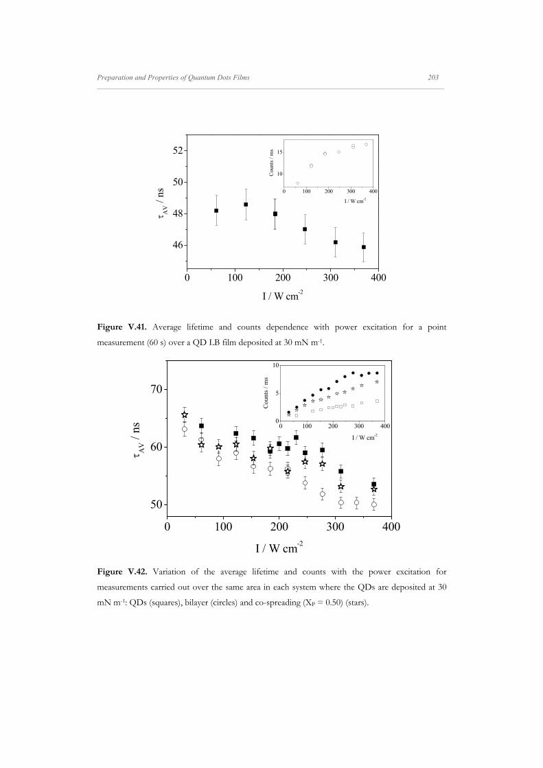
Preparation and Properties of Quantum Dots Films 203 _____________________________________________________________________________________________________________________
0 100 200 300 400
46
48
50
52
0 100 200 300 400
10
15
AV /
ns
I / W cm-2
Cou
nts
/ ms
I / W cm-2
Figure V.41. Average lifetime and counts dependence with power excitation for a point
measurement (60 s) over a QD LB film deposited at 30 mN m-1.
0 100 200 300 400
50
60
70
0 100 200 300 4000
5
10
AV /
ns
I / W cm-2
Cou
nts
/ ms
I / W cm-2
Figure V.42. Variation of the average lifetime and counts with the power excitation for
measurements carried out over the same area in each system where the QDs are deposited at 30
mN m-1: QDs (squares), bilayer (circles) and co-spreading (XP = 0.50) (stars).

204 Preparation and Properties of Quantum Dots Films _____________________________________________________________________________________________________________________
0 100 200 300 40030
40
50
60
70
0 100 200 300 4000
1
2
3
AV /
ns
I / W cm-2
Cou
nts
/ ms
I / W cm-2
Figure V.43. Variation of the average lifetime and counts with the power excitation (energy ramp)
for measurements carried out over the same area in co-spread (XP = 0.65) systems where the QDs
are deposited at 14 (open symbols) and 30 (closed symbols) mN m-1.
In summary, these experiments have allowed us to analyze the effect of
excitation energy on LB films. The average lifetime value decreases when the
power laser is increased due to a multi-exciton formation. In order to avoid multi-
excitonic relaxation processes that interfere in the analysis of the QDs PL
dynamics, we decided to measure at a low power excitation, 108 W cm-2, which at
the same time allows us to collect a PL decay with sufficient intensity counts to
minimize experimental uncertainty. In the case of the power energy selected, we
estimated that the formation of multi-excitonic states is low, ca. 3.1% (Figure
V.42c).
V.4.3.3. Effect of the Exposure Time on QDs LB films
In order to analyze the effect of the exposure time on the PL decay we
carried out several experiments by modifying this time. We performed two
different sets of measurements over points and areas. The point measurements in
different samples show that the PL decays vary during the exposure time,
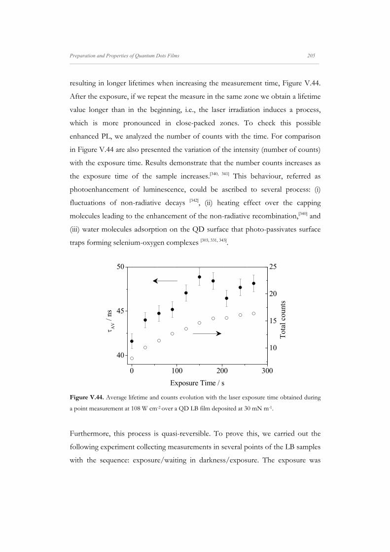
Preparation and Properties of Quantum Dots Films 205 _____________________________________________________________________________________________________________________
resulting in longer lifetimes when increasing the measurement time, Figure V.44.
After the exposure, if we repeat the measure in the same zone we obtain a lifetime
value longer than in the beginning, i.e., the laser irradiation induces a process,
which is more pronounced in close-packed zones. To check this possible
enhanced PL, we analyzed the number of counts with the time. For comparison
in Figure V.44 are also presented the variation of the intensity (number of counts)
with the exposure time. Results demonstrate that the number counts increases as
the exposure time of the sample increases.[340, 341] This behaviour, referred as
photoenhancement of luminescence, could be ascribed to several process: (i)
fluctuations of non-radiative decays [342], (ii) heating effect over the capping
molecules leading to the enhancement of the non-radiative recombination,[340] and
(iii) water molecules adsorption on the QD surface that photo-passivates surface
traps forming selenium-oxygen complexes [303, 331, 343].
0 100 200 300
40
45
50
10
15
20
25
AV /
ns
Exposure Time / s
Tot
al c
ount
s
Figure V.44. Average lifetime and counts evolution with the laser exposure time obtained during
a point measurement at 108 W cm-2 over a QD LB film deposited at 30 mN m-1.
Furthermore, this process is quasi-reversible. To prove this, we carried out the
following experiment collecting measurements in several points of the LB samples
with the sequence: exposure/waiting in darkness/exposure. The exposure was

206 Preparation and Properties of Quantum Dots Films _____________________________________________________________________________________________________________________
performed at different power excitations and therefore, the exposure time was
increased when a lower power excitation is used to achieve a similar effect. The
experimental procedure was the following: first, we take a FLIM image of the
zone (A) and then record the point measurement (τI, 1st exposure); immediately
after, we take other FLIM image of the zone (B) and left the sample at darkness
(shutter closed) during 30 min; just after, we take the third image (C) and make
other point measurement (τII, 2nd exposure) followed by the last FLIM image
capture (D). Thus, in these measurements we recorded the images of the zone at
the beginning and end of every period of laser irradiation and darkness waiting
period steps (30 min). As an example of the point laser exposure effect on the
samples, images of two different samples are shown in Figure V.45. After the laser
exposure the affected zone change in the colour scale (lifetime) from green to red
indicating an increasing in the lifetime. After waiting 30 min, we checked again the
zone, and the observed colour highlights a partial recover to the initial state, less
coloured red zone. The waiting time in darkness was established after several
proofs of successive 5 min waits and image captures. The effect in the image
becomes noticeable after 30 min, thus it is enough time to observe the behaviour
ensuring that the scanner position is kept stable.

Preparation and Properties of Quantum Dots Films 207 _____________________________________________________________________________________________________________________
Figure V.45. FLIM images showing the evolution of the exposed zone to laser irradiation (a, e)
zone selected; (b, f) after 5 min exposed (first laser irradiation); (c, g) after waiting 30 min; (d, h)
after 5 min exposed (second laser irradiation). The experimental conditions were: 430 W cm-2
applied over a selected point. The images correspond to: bilayer (a-d) and co-spreading (XP = 0.50)
(e-h) prepared at the surface pressure of 30 mN m-1.
The photo-induced process is quasi-reversible. To confirm this qualitative
observation, we analyze the average lifetime, τji at the different stages of the
experiment, where i, indicates the time range of laser illumination evaluated in the
decay curve and j the number of exposure. We evaluated the average lifetime
acquired at regular intervals during each illumination period to have an idea of the
sample point state at each moment. Our results show that τIbeginning < τI
end
highlighting the photoenhancement behaviour previously mentioned. Other fact
observed is that τIend > τII
beginning > τIbeginning, consistent with a quasi-reversible
process: the average lifetime for the initial state after waiting (2nd exposure) is
lower than the corresponding to the final state after the 1st exposure. In summary,
the average lifetime values and images (Table V.6, Figure V.45), both, agree with
the idea that the laser illumination induces a quasi-reversible process. After the
waiting in darkness, the average lifetime is decreased but it does not recover to the
initial value (sample state). In the case of the images, the colour of the zone
around the point exposed changes but never gets back to the initial state. This
a b c d
e f g h2 µm
2 µm
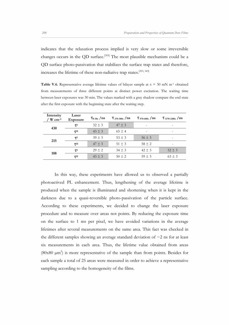
208 Preparation and Properties of Quantum Dots Films _____________________________________________________________________________________________________________________
indicates that the relaxation process implied is very slow or some irreversible
changes occurs in the QD surface.[303] The most plausible mechanism could be a
QD surface photo-passivation that stabilizes the surface trap states and therefore,
increases the lifetime of these non-radiative trap states.[303, 343]
Table V.6. Representative average lifetime values of bilayer sample at π = 30 mN m-1 obtained
from measurements of three different points at distinct power excitation. The waiting time
between laser exposures was 30 min. The values marked with a gray shadow compare the end state
after the first exposure with the beginning state after the waiting step.
Intensity / W cm-2
Laser Exposure τ0-30s /ns τ 270-300s /ns τ 570-600s /ns τ 1170-1200s /ns
430 τI 32 ± 3 47 ± 3 - -
τII 43 ± 3 65 ± 4 - -
215 τI 39 ± 3 53 ± 3 56 ± 3 -
τII 47 ± 3 51 ± 3 58 ± 2 -
108 τI 29 ± 2 34 ± 3 42 ± 3 52 ± 3
τII 43 ± 3 50 ± 2 59 ± 3 63 ± 3
In this way, these experiments have allowed us to observed a partially
photoactived PL enhancement. Thus, lengthening of the average lifetime is
produced when the sample is illuminated and shortening when it is kept in the
darkness due to a quasi-reversible photo-passivation of the particle surface.
According to these experiments, we decided to change the laser exposure
procedure and to measure over areas not points. By reducing the exposure time
on the surface to 1 ms per pixel, we have avoided variations in the average
lifetimes after several measurements on the same area. This fact was checked in
the different samples showing an average standard deviation of ~2 ns for at least
six measurements in each area. Thus, the lifetime value obtained from areas
(80x80 µm2) is more representative of the sample than from points. Besides for
each sample a total of 25 areas were measured in order to achieve a representative
sampling according to the homogeneity of the films.
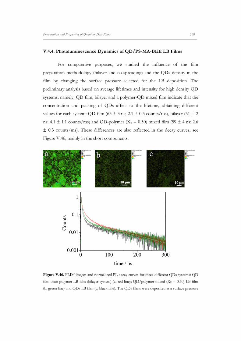
Preparation and Properties of Quantum Dots Films 209 _____________________________________________________________________________________________________________________
V.4.4. Photoluminescence Dynamics of QD/PS-MA-BEE LB Films
For comparative purposes, we studied the influence of the film
preparation methodology (bilayer and co-spreading) and the QDs density in the
film by changing the surface pressure selected for the LB deposition. The
preliminary analysis based on average lifetimes and intensity for high density QD
systems, namely, QD film, bilayer and a polymer-QD mixed film indicate that the
concentration and packing of QDs affect to the lifetime, obtaining different
values for each system: QD film (63 ± 3 ns; 2.1 ± 0.5 counts/ms), bilayer (51 ± 2
ns; 4.1 ± 1.1 counts/ms) and QD-polymer (XP = 0.50) mixed film (59 ± 4 ns; 2.6
± 0.3 counts/ms). These differences are also reflected in the decay curves, see
Figure V.46, mainly in the short components.
0 100 200 3001E-3
0.01
0.1
1
Cou
nts
time / ns
0.001
Figure V.46. FLIM images and normalized PL decay curves for three different QDs systems: QD
film onto polymer LB film (bilayer system) (a, red line); QD/polymer mixed (XP = 0.50) LB film
(b, green line) and QDs LB film (c, black line). The QDs films were deposited at a surface pressure
10 µm10 µm10 µm
a b c

210 Preparation and Properties of Quantum Dots Films _____________________________________________________________________________________________________________________
of 30 mN m-1. Solid lines in grey colour show the fitting results with a multi-exponential decay
analysis.
To confirm that the decay curves obtained from different regions within
each sample agree with each other, we analyzed several PL decays in distinct areas.
An illustrative example is shown in Figure V.47, where three different regions of
the same sample are presented. The respective curves agree with each other.
Therefore the average lifetime values obtained are representative of each system.
0 100 200 3001E-3
0.01
0.1
1
30 40 50 60 700
5
10
Occ
urre
nce
AV
/ ns0 2 4 6 8 10
0
5
10
15
Occ
urre
nce
Counts /ms
Cou
nts
time / ns
0.001
Figure V.47. Comparative FLIM images and normalized PL decay curves for the bilayer system
over three different areas for each side of the lifetime values distribution: low (green line), medium
(black line) and high (red line) respectively. The histograms show the lifetime and counts
distribution in this sample.
10 µm 10 µm 10 µm

Preparation and Properties of Quantum Dots Films 211 _____________________________________________________________________________________________________________________
On the other hand, the dark zones observed in the FLIM images corresponding
to regions not covered were checked, and no emission was observed.
We also analyze the effect of the surface composition on the emission
properties. Thus, LB films of QD/PS-MA-BEE were prepared at different
polymer mole fractions, XP = 0.35, 0.50 and 0.65 at the surface pressure of 30 mN
m-1. By comparing the decays of the different co-spreading films shown in Figure
V.48, we observe that the main differences are in the slowest component. This
behaviour suggests that a different arrangement of QDs is obtained by varying the
polymer concentration The average lifetime and intensity counts values of each
system highlight this behaviour: (XP = 0.50) (59 ± 4 ns; 2.6 ± 0.3 counts/ms); (XP
= 0.65) (48 ± 3 ns; 1.0 ± 0.1 counts/ms) and (XP = 0.35) (44 ± 6 ns; 1.3 ± 0.3
counts/ms).
0 100 200 3001E-3
0.01
0.1
1
(XP = 0.35)
(XP = 0.50)
Cou
nts
time / ns
(XP = 0.65)
0.001
Figure V.48. Comparative normalized PL decay curves for three different QD-polymer mixed LB
film at high surface pressure (30 mN m-1) with a polymer mole fraction: (0.35) (black line); (0.50)
(green line) and (0.65) (blue line).

212 Preparation and Properties of Quantum Dots Films _____________________________________________________________________________________________________________________
The effect of the surface pressure in the PL decays was also studied. As is
shown in Figure V.49 at low surface pressure the film PL decays point to a lower
contribution in the slow components corroborated by the lifetime average values:
(XP = 0.65) (48 ± 4 ns; 0.8 ± 0.1 counts/ms) and (XP = 0.35) (31 ± 6 ns; 0.9 ± 0.1
counts/ms).
0 100 200 3001E-3
0.01
0.1
1 a
Cou
nts
time / ns
high
low
0.001
0 100 200 3001E-3
0.01
0.1
1 b
high
Cou
nts
time / ns
low
0.001
Figure V.49. Comparative normalized PL decay curves for two different QD-polymer LB systems
at low (gray line) and high (black line) surface pressure (14 and 30 mN m-1) with a molar ratio: (XP
= 0.35) (a) and (XP = 0.65) (b).
As was mentioned the PL decays were analyzed by a multi-exponential
function that requires four exponential components to be properly fitted. Results
are collected in Table V.7.

Preparation and Properties of Quantum Dots Films 213 _____________________________________________________________________________________________________________________
Table V.7. Results from multi-exponential decay analysis for area measurement over LB films at
108 W cm-2. The reduced chi-square values, χ2, all close to 1, and the weighted residuals indicate a
good fit to each data set. Data obtained from measurements over at least 25 areas for each sample. High π
QDs Bilayer Co-spr
(XP = 0.50) Co-spr
(XP = 0.65) Co-spr
(XP = 0.35) τ1 / ns 0.12 ± 0.04 0.15 ± 0.02 0.15 ±0.02 0.14 ±0.02 0.19 ±0.05 f1 (%) 19 ±4 10 ±1 12 ±1 16 ±2 16 ±5 τ2 / ns 2.0 ±0.1 2.60 ±0.08 2.15 ±0.07 2.0 ±0.1 2.4 ±0.2 f2 (%) 17 ±2 16.6 ±0.6 20 ±1 22 ±2 29 ±3 τ3 / ns 9 ±1 14.2 ±0.5 10.3 ±0.6 9 ±1 11 ±1 f3 (%) 15 ±2 27 ±1 17.5 ±0.6 20 ±1 21 ±2 τ4 / ns 123 ±5 102 ±3 118 ±4 114 ±7 116 ±6 f4 (%) 48 ± 3 46 ± 2 50 ± 2 42 ± 3 35 ± 3 τAV / ns 63 ± 3 51 ± 2 59 ± 4 48 ± 3 44 ± 6 Counts/ms 2.1 ± 0.5 4.1 ± 1.1 2.6 ± 0.3 1.0 ± 0.1 1.3 ± 0.3
Low πCo-spr
(XP = 0.65) Co-spr
(XP = 0.35) τ1 / ns 0.13 ±0.04 0.16 ±0.07 f1 (%) 18 ± 3 26 ±4τ2 / ns 1.9 ±0.2 2.0 ±0.2 f2 (%) 26 ±3 31 ±3τ3 / ns 6.9 ±0.8 7.0 ±0.9 f3 (%) 22 ±2 21 ±2τ4 / ns 119 ±10 124 ±10 f4 (%) 34 ± 4 21 ± 3τAV / ns 48 ± 4 31 ± 6 Counts/ms
0.8 ± 0.1 0.9 ± 0.1
In the time range analyzed, the decays exhibit a pronounced curvature that
is clearly distinct for films prepared by bilayer and co-spreading deposition, see
Figure V.46. The results from the multi-exponential analysis of film decays
indicate that the results obtained for the bilayer film stand out, because the
averaged short decay times are clearly longer than for co-spreading films, while
the long decay time is quite similar for all samples prepared by the two deposition
methods. Later, we will relate the former observation to differences in film
morphology.

214 Preparation and Properties of Quantum Dots Films _____________________________________________________________________________________________________________________
On the other hand, the relative brightness (counts) of the PL images also
reflects the difference between bilayer and co-spreading films. Under the same
excitation conditions, the bilayer films have a significantly higher intensity of
emission compared to co-spreading films, i.e. a larger number of counts per
image. This observation could be simply due to a higher surface concentration of
QDs in the bilayer films. To disregard this point, the emission intensity is plotted
against the particle density calculated from surface concentration, in Figure V.50.
The surface concentration was calculated from the π-Γ isotherms at the surface
pressure of LB deposition and expressed in number of QDs per area. Results in
Figure V.50 show that the PL intensity of the co-spreading films is proportional
to particle density, while the PL intensity of the bilayer film stands out, indicating
that it is much more emissive than the co-spreading film with the same particle
density.
0 10 20 30 400.0
0.4
0.8
1.2
1.6
PL I
nten
sity
(10
6 cou
nts
per
imag
e)
Surface concentration (103 dots / m2)
1
2
34 56
Figure V.50. Emission intensity from PL images vs. surface concentration of QDs calculated
from the corresponding π-Γ isotherms for the bilayer (1) and co-spreadings (XP = 0.50) (2); (XP =
0.65) (3, 5) and (XP = 0.35) (4, 6). Closed and open symbols represent data from films deposited at
high and low surface pressures, 30 and 14 mN m-1, respectively.
Preparation and Properties of Quantum Dots Films 215 _____________________________________________________________________________________________________________________
V.4.4.1. Interpretation of the QDs Photoluminescence Dynamics
As was previously mentioned, the PL dynamics of QDs in the ns–µs
timescale are intrinsically complex due to the role of surface defect and charge
trapped states in excited-state relaxation.[319, 344-347] In the solid films, the
complexity is further increased by the possibility of excitation energy transfer
between QDs, because of the short interparticle distances in the closely-packed
film regions. Accordingly, several processes are involved in QD photoexcitation
dynamics that are depicted in a schematic diagram in Figure V.51. In addition to
radiative recombination process, there are other competing processes from the
excited state such as the carrier trapping at QD surface defects, ked; charge transfer
into ligand-based orbitals, kct, and relaxation to the ground state, kdg and kbg. The
QD surface defect states strongly quench emission from band-edge exciton
recombination, ked, promoting faster excited-state decay. The surface defects can
be arisen from native defect such as metal vacancies or dangling ligand bonds[348]
and can be also related to detachment of ligand molecules as occurs in diluted QD
solutions[335]. Other non-radiative recombination processes such as hot carrier
relaxation and multi-excitonic processes can also contribute to ultrafast excited-
state decay. Furthermore, in QD films the complexity is increased by the
possibility of energy migration and trapping between QDs due to a compact
particle arrangement in densely covered regions. Besides, the formation of small
QD clusters, which act as energy traps together with QD surface defects, and the
compact particle arrangement also promotes luminescence quenching due to
stabilization of non-emissive charged states by Coulomb interactions between
clustered QDs [320, 349-351] [349] [320, 350]. The Coulombic stabilization of charged states
only induces quenching if it favours charge recombination to ground state, kbe,
relative to excited state. Finally, the delayed luminescence from charge transfer
and trapping in the surrounding environment of the QD (kct and kbe) occurs and is
the main contribution from isolated QDs or compact regions without traps,
which do not suffer emission quenching. This emission explains the exponential

216 Preparation and Properties of Quantum Dots Films_____________________________________________________________________________________________________________________
behaviour observed in the PL decays from about a hundred ns onward and is
associated to a slow decay rate.
Figure V.51. A simplified schematic diagram of several processed involved in QD photoexcitation
dynamics adapted from (Jones, 2010 [25]).
Prior to the decay analysis, we describe our qualitative interpretation of the
film decays, which is based on this model and the broad literature about PL
dynamics of QDs and their solid films. We attribute the sharp decrease in the
initial nanoseconds to QDs with extensive surface defects that strongly quench
emission from band-edge exciton recombination (‘ked’ in Figure V.51).[334, 335]
Within an ensemble of QDs, the surface conditions vary among the particles, and
more likely there is a statistical distribution of the number of surface defects per
particle. We hypothesize that a small fraction of QDs with extensive surface
defects can act as excitation energy traps in our ensemble of deposited QDs in the
films, as it is further discussed below.
Because the emission from surface defect states is usually observed at
lower energies relatively to core exciton recombination (‘kdg’ in Figure V.51), we
perform PL spectral measurements. Taking into account that the QD emission
from core and trap states are spectrally separable, these experiments allow us to
select the emission wavelength range. The collection of both spectral features in
Radiativedecay
+-
chargetrapped
statessurfacedefectstates
kct
kbe
ked
kdg
kbgτr
GROUND STATE
EXCITED STATE
Non-radiativerecombination

Preparation and Properties of Quantum Dots Films 217 _____________________________________________________________________________________________________________________
the same time-trace makes the PL decay analysis more difficult.[346] In order to
obtain evidences, we record the PL emission at different wavelength ranges, at the
blue and red sides of the PL QDs spectrum maximum. The wavelength selection
is carried out using several band-pass filters placed in front of avalanche
photodiodes.
The emission spectra of the QDs dissolved in chloroform and in LB film
were recorded. As Figure V.52 shows, the QDs PL spectra consist of two
emission bands: a sharp band-edge at ~580 nm and a broad non-structured band
at longer wavelength. The band-edge emission is due to core recombination of the
exciton in the mostly delocalized states in QDs, while the broad band is ascribed
to the trap-state emission and due to surface defects on the interface between the
nanoparticle and the surrounding medium.[343, 344, 352] In the case of QDs in
solution, Figure V.52a shows the core recombination emission band, centred at ~
580 nm, and the broad non-structured band centred at wavelengths longer than ~
700 nm. It is interesting to note that the intensity corresponding to surface defect
states band is much lower than the one corresponding to the core recombination
band. This fact could indicate that no significant interference occurs from the
surface defects’ emission on the decay curves. In the case of QDs LB films,
Figure V.52b, the core exciton recombination band is also centred at ~ 580 nm,
but the main difference occurs in the surface defect emission band centred at ~
620 nm, which is more pronounced in the films than in solution. This
predominance of surface defect emission band in the spectra of QDs films has
been observed by other authors.[340]
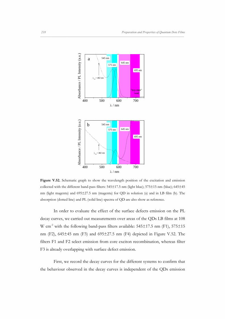
218 Preparation and Properties of Quantum Dots Films _____________________________________________________________________________________________________________________
400 500 600 700
575 nm
695 nm
645 nm
Abs
orba
nce
/ PL
Int
ensi
ty (
a.u.
)
/ nm
545 nma
"trap-state" band
exc
= 482 nm
400 500 600 700
575 nm
695 nm
645 nm
Abs
orba
nce
/ PL
Int
ensi
ty (
a.u.
)
/ nm
545 nm
exc
= 482 nm
b
Figure V.52. Schematic graph to show the wavelength position of the excitation and emission
collected with the different band-pass filters: 545±17.5 nm (light blue); 575±15 nm (blue); 645±45
nm (light magenta) and 695±27.5 nm (magenta) for QD in solution (a) and in LB film (b). The
absorption (dotted line) and PL (solid line) spectra of QD are also show as reference.
In order to evaluate the effect of the surface defects emission on the PL
decay curves, we carried out measurements over areas of the QDs LB films at 108
W cm-2 with the following band-pass filters available: 545±17.5 nm (F1), 575±15
nm (F2), 645±45 nm (F3) and 695±27.5 nm (F4) depicted in Figure V.52. The
filters F1 and F2 select emission from core exciton recombination, whereas filter
F3 is already overlapping with surface defect emission.
First, we record the decay curves for the different systems to confirm that
the behaviour observed in the decay curves is independent of the QDs emission
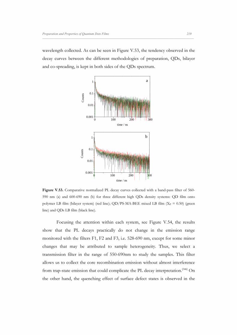
Preparation and Properties of Quantum Dots Films 219 _____________________________________________________________________________________________________________________
wavelength collected. As can be seen in Figure V.53, the tendency observed in the
decay curves between the different methodologies of preparation, QDs, bilayer
and co-spreading, is kept in both sides of the QDs spectrum.
0 100 200 3001E-3
0.01
0.1
1
Cou
nts
time / ns
a
0.001
0 100 200 3001E-3
0.01
0.1
1
Cou
nts
time / ns
b
0.001
Figure V.53. Comparative normalized PL decay curves collected with a band-pass filter of 560-
590 nm (a) and 600-690 nm (b) for three different high QDs density systems: QD film onto
polymer LB film (bilayer system) (red line); QD/PS-MA-BEE mixed LB film (XP = 0.50) (green
line) and QDs LB film (black line).
Focusing the attention within each system, see Figure V.54, the results
show that the PL decays practically do not change in the emission range
monitored with the filters F1, F2 and F3, i.e. 528-690 nm, except for some minor
changes that may be attributed to sample heterogeneity. Thus, we select a
transmission filter in the range of 550-690nm to study the samples. This filter
allows us to collect the core recombination emission without almost interference
from trap-state emission that could complicate the PL decay interpretation.[346] On
the other hand, the quenching effect of surface defect states is observed in the

220 Preparation and Properties of Quantum Dots Films _____________________________________________________________________________________________________________________
initial part of the decay curves, as a fast decay component previously referred.
This fast quenching process is out of the main scope of this work and, therefore,
in the data analysis the initial part of the decay curves, t < 10 ns, was neglected
and the analysis was focused to the longest components also attributed to
emission from core exciton recombination.
0 10 20 300.01
0.1
1
545 nm
695 nm
645 nm
575 nm
Cou
nts
time / ns
a
0 100 200 3001E-3
0.01
0.1
1 b
575 nm 645 nm
545 nm
695 nm
Cou
nts
time / ns
0.001
0 10 20 300.01
0.1
1 c
Cou
nts
time / ns
575 nm
645 nm545 nm
695 nm
0 100 200 3001E-3
0.01
0.1
1 d
Cou
nts
time / ns
575 nm
645 nm545 nm
695 nm
0.001
0 10 20 300.01
0.1
1 e
Cou
nts
time / ns
575 nm 645 nm
545 nm
695 nm
0 100 200 3001E-3
0.01
0.1
1 f
Cou
nts
time / ns
575 nm
645 nm
545 nm
695 nm
0.001
Figure V.54. Comparative normalized PL decay curves collected with different band-pass filters
of 528-563 nm (dark gray line); 560-590 nm (light gray line); 600-690 nm (black line) and 668-723
nm (gray line) at 108 W cm-2 for a QDs (a, b); bilayer (c, d) and co-spread (XP = 0.50) (e, f) LB
films where the QDs are deposited at 30 mN m-1.

Preparation and Properties of Quantum Dots Films 221 _____________________________________________________________________________________________________________________
Finally, when we collect the emission decay in the range of surface defect
emission [343, 344, 352, 353] with the filter F4 that has a transmission window between
668-723 nm, slower components appear either in solution, Figure V.55, and LB
films. This behaviour is characteristic of the surface-defect emission.[352, 353]
0 100 200 3001E-3
0.01
0.1
1
Cou
nts
time / ns
695 nm
645 nm
0.001
Figure V.55. Comparative normalized PL decay curves collected with different band-pass filters
of 600-690 nm (black line) and 668-723 nm (gray line) at 67 W cm-2 for a QDs chloroform
solution.
In summary, the photoluminescence spectral measurements collected in
different zones of the QD spectrum allowed us to discard significant interference
from the surface defects emission on the decay curves in the wavelength range
selected. In this sense, the behaviour observed at long spectral wavelengths
highlighted the surface-defects emission and allows us to ensure that the
conditions selected to work are not almost influenced for this emission and collect
the core-recombination emission.
Going back to the study of the effect of the films morphology on the
photoluminescence properties, in an attempt to interpret the differences between
the emission properties of co-spreading and bilayer films, the TEM images of

222 Preparation and Properties of Quantum Dots Films _____________________________________________________________________________________________________________________
these films were analyzed. Representative TEM images are shown in Figure V.56.
The TEM images show regions densely covered along with other regions more
sparsely covered. Overall, the bilayer film shows a more regular particle
distribution than co-spreading films. It is also noticeable the presence of small
densely packed clusters of QDs, which could act as excitation energy traps. This
idea is supported by previous results that reported the existence of luminescence
quenching and enhanced blinking occurs in small QD clusters.[320] The
stabilization of non-emissive charged states by Coulomb interactions between
clustered QDs seems to be responsible for this behaviour.[320, 349-351].
Figure V.56. Examples of TEM images obtained for bilayer (a) and co-spreading deposition with
a QD-polymer molar ratio of XP = 0.50 (b) XP = 0.65 (c) and XP = 0.35 (d) at high pressure, π =
30 mN m-1; and co-spreading with ratios of XP = 0.65 (e) and XP = 0.35 (f) at low pressure, π = 14

Preparation and Properties of Quantum Dots Films 223 _____________________________________________________________________________________________________________________
mN m-1. The area shown in TEM images corresponds approximately to about 1 pixel in the FLIM
images.
The PL dynamics of the films are affected by the surface distribution of
particles, because in the regions densely covered the interparticle distances are
only a few nm and dot-dot excitation energy transfer is likely to occur within the
ensemble of closely packed particles. The migration of excitation energy affects
the observed decay because of sample heterogeneity and, in particular, due to
excitation energy traps that are commonly present in solid films. We attribute the
role of energy traps in our films to QDs with extensive surface defects and to
small aggregated QDs clusters, as mentioned above.
From about a hundred ns onward, the decays show an almost exponential
behaviour that is attributed to isolated QDs or to closely-packed regions without
energy traps, which do not suffer emission quenching. The PL of the QDs decays
very slowly with lifetime components longer than hundred ns, and even reaching
µs in chloroform solution. The long decay tail observed in the PL of QDs has
been attributed in the literature to a process of delayed luminescence from charge
transfer and trapping in the surrounding environment of the quantum dot.[345, 346]
Furthermore, it has also been associated with the power-law statistics of emission
intermittency of single-dots observed in the timescale of ms to s.[345, 354, 355] We
assume that delayed luminescence from charge transfer and trapping in the
surrounding environment is also responsible for the long decay tail observed in
the emission of our QDs (‘kct’ and ‘kbe’ in Figure V.51).
Alternatively to the multi-exponential analysis of QDs film decays, we
have adopted an approximate model to describe the PL dynamics in QD/polymer
films, in particular, the excitation energy migration and trapping processes in the
densely covered regions. The model considers two separate contributions from
sparse and compact regions of immobilized QDs in the films. This picture is
supported by the TEM images that show regions compactly covered with QDs

224 Preparation and Properties of Quantum Dots Films _____________________________________________________________________________________________________________________
along with other regions more sparsely covered. Therefore, the decay function
assumes two terms, and , that account separately for sparse and
compact regions of QDs,
1 V. 1
The term describes the intrinsic photophysics of QDs, which can be very
complex because core exciton states often interact with surface localized states
and the surrounding environment. In organically coated QDs, this type of
interaction can result in charge trapping on surface defect sites, or on ligand-based
orbitals, with the formation of an ionized core state that is usually non-emissive.
Therefore, charge transfer and trapping in the surrounding environment have an
important role in excited-state relaxation of QDs.[345, 346] On the other hand, the
term further accounts for interparticle energy migration and trapping
processes, because it describes the contribution from compact film regions. An
overview on the models selected for and , and their respective
parameters, is explained below. The term was assumed to be described by
the Tachiya-Mozumder model.[355, 356] This model considers a mechanism of
charge trapping by electron tunneling toward an uniform distribution of traps.
The decay function is calculated by numerical Laplace inversion of,
11 r⁄ ct
V. 2
with three adjustable parameters, the radiative recombination rate , the charge
transfer rate term , and a power-law exponent 1 . A value of 30 ns was
taken as initial guess for r in the fittings. This value was estimated from the r
fitted for decays of QDs dissolved in chloroform solution and corrected for the
dielectric screening in the films. The charge transfer rate term was varied to
fit the long time behaviour of the film decays. The initial guess for the power-law
exponent 1 ~ 2 was also based on our results of luminescence decays of QDs

Preparation and Properties of Quantum Dots Films 225 _____________________________________________________________________________________________________________________
in chloroform. Using 1 ~ 2, or equivalently ~ 1, then by Laplace inversion
of Equation V.2,
exp r 1 ct⁄ V. 3
Here, we notice that Equation V.3 predicts a decay law exponential, in agreement
with results observed at long times in the decays of Figure V.46.
For the term in Equation V.1 we have adopted results from the
theoretical method of diagrammatic expansion of the Green's function developed
by Fayer and co-workers.[357, 358] In the case of a two-dimensional random
distribution of donors and traps that interact through a dipolar transfer rate, the
Green's function s ′, for the probability that excitation is on the initially
excited site at time is given by the following self-consistent equation in Laplace
domain,
s 2 ⁄ 3 ⁄D⁄
D 2 ⁄T
s ⁄1⁄ 0 V. 4
with D, the donor lifetime, D and T, the donor and trap reduced
concentrations, as described below. From Equation 4 the probability D that
an excitation is in the donor ensemble at time is obtained from inverse
transform of,
D 0, s 1 2 ⁄ D 3 ⁄D⁄ s ⁄
V. 5
The corresponding decay law is obtained multiplying D by a decaying
exponential with the donor lifetime,
exp D⁄ D V. 6
When fitting the decays, we have assumed the approximation in Equation
3 for the individual QD decay in the timescale of hundreds of ns, which implies
that the donor lifetime is D~ r 1 ct . The reduced concentrations D and
T are defined by,
DDD
D , TDT
T V. 7
226 Preparation and Properties of Quantum Dots Films _____________________________________________________________________________________________________________________
with DD and DT, the Förster radius for donor-donor and donor-trap energy
transfer, D and T, the number densities of donors and traps, respectively.
Although the interparticle distance is comparable with the QD size, it has been
shown that the dipolar approximation in Förster theory describes reasonably well
the excitation energy transfer between QDs or even between QD and fluorescent
molecules.[359, 360] Using the theory, we estimate a Förster radius DD of 4.1 nm for
donor-donor energy transfer and assume a similar DT value for donor-trap
energy transfer. However, when fitting the decays no assumption was made about
DD and DT values by treating D and T as the adjustable parameters.
The decays of our QDs films are only approximately described by
Equation V.1 mainly because of two reasons: i) at very short times (below ten ns),
the surface defect states contribute predominantly to fast excited-state decay; and
ii) the model considered for the compact regions, , does not account for
boundary effects due to finite domain size. In spite of these limitations, the
approximate description of Equation V.1 allows to rationalize the
photoluminescence dynamics of the QDs films using only a few adjustable
parameters that afford physical insight about the systems studied.
The parameters obtained from fittings with Equation V.1 to the decays of
bilayer and co-spreading films are collected in Table V.8. For instance, the bilayer
film exhibits a decay curvature in the time range up to a hundred ns that is less
pronounced than those of co-spreading films. Accordingly, the concentration of
traps T for the bilayer film is about half of that from co-spreading films.
Moreover, the concentration of donors D is approximately the same for both
systems and it is close to the value of 3.3 particles within the area of a Förster
radius. This corresponds to a dense arrangement of QDs in the compact domains
as observed in TEM images. Indeed, considering the estimated Förster radius of
4.1 nm and the QD average size of 3.5 nm, then a hexagonal compact
arrangement would be achieved for a interparticle surface-to-surface distance of
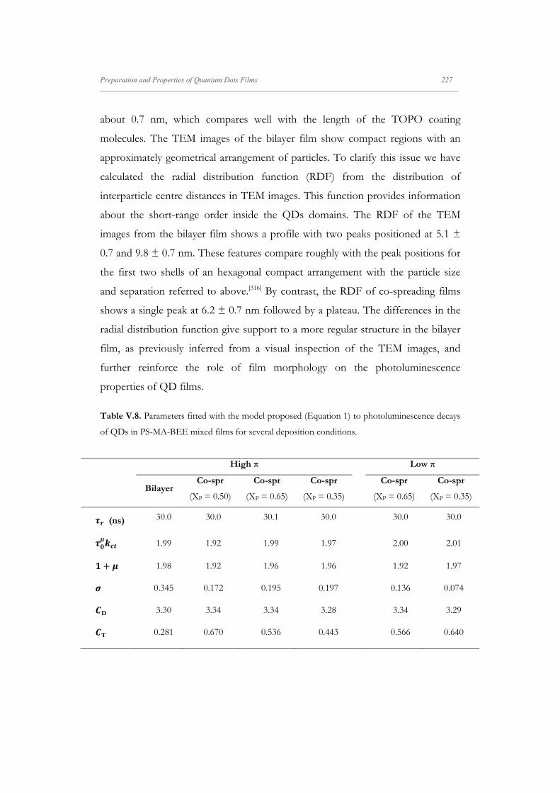
Preparation and Properties of Quantum Dots Films 227 _____________________________________________________________________________________________________________________
about 0.7 nm, which compares well with the length of the TOPO coating
molecules. The TEM images of the bilayer film show compact regions with an
approximately geometrical arrangement of particles. To clarify this issue we have
calculated the radial distribution function (RDF) from the distribution of
interparticle centre distances in TEM images. This function provides information
about the short-range order inside the QDs domains. The RDF of the TEM
images from the bilayer film shows a profile with two peaks positioned at 5.1 ±
0.7 and 9.8 ± 0.7 nm. These features compare roughly with the peak positions for
the first two shells of an hexagonal compact arrangement with the particle size
and separation referred to above.[316] By contrast, the RDF of co-spreading films
shows a single peak at 6.2 ± 0.7 nm followed by a plateau. The differences in the
radial distribution function give support to a more regular structure in the bilayer
film, as previously inferred from a visual inspection of the TEM images, and
further reinforce the role of film morphology on the photoluminescence
properties of QD films.
Table V.8. Parameters fitted with the model proposed (Equation 1) to photoluminescence decays
of QDs in PS-MA-BEE mixed films for several deposition conditions.
High π Low π
Bilayer Co-spr
(XP = 0.50)
Co-spr
(XP = 0.65)
Co-spr
(XP = 0.35)
Co-spr
(XP = 0.65)
Co-spr
(XP = 0.35)
(ns) 30.0 30.0 30.1 30.0 30.0 30.0
1.99 1.92 1.99 1.97 2.00 2.01
1.98 1.92 1.96 1.96 1.92 1.97
0.345 0.172 0.195 0.197 0.136 0.074
D 3.30 3.34 3.34 3.28 3.34 3.29
T 0.281 0.670 0.536 0.443 0.566 0.640

228 Preparation and Properties of Quantum Dots Films _____________________________________________________________________________________________________________________
The decays from both bilayer and co-spreading films are approximately
exponential at long times with the same slope (Figure V.46). Thus, the model
parameters , , and 1 describing the decay of isolated QDs or
domains without energy traps, , are similar for bilayer and co-spreading films.
Only the relative contribution to the decay, , is different with the bilayer film
having a larger contribution of 34.5 % compared to 17.2 % in the QD-polymer
co-spreading film with XP = 0.50. We relate the larger contribution of in
bilayer deposition to a film structure that contains a lower number of small
aggregated QDs clusters that act as energy traps. The cluster formation has been
previously studied and was attributed to dewetting processes. The current work
further supports that nanoparticle clustering acts as energy traps thereby reducing
the PL emission, as it was proposed elsewhere.[320]
To evaluate the effect of the polymer concentration on the luminescence
properties, the photoluminescence decays of films with different polymer mole
fraction were analyzed according to the Equation V.1. The QD/polymer
compositions selected were XP = 0.35, 0.50 and 0.65. The parameter values
obtained from the decay fits show no significant differences, except for a small
increase of the contribution when the polymer mole fraction increases. More
significant is the emission brightness observed in these films that is related to the
distinct surface density of QDs as was previously noticed in the Figure V.50.
The effect of surface pressure in co-spreading deposition was also
evaluated. The fitted parameters obtained for decays curves of films prepared by
co-spreading method and surface pressure of 14 mN m-1 are collected in Table
V.8. From the parameter values it is possible to conclude that at low pressure the
film decays have a lower contribution from the long time exponential component
(Figure V.49), while the rest of fitted parameters are almost independent of the
polymer mole fraction. The decrease of the emission intensity found in these films

Preparation and Properties of Quantum Dots Films 229 _____________________________________________________________________________________________________________________
is also consistent with the decrease of the QDs surface concentration (Figure
V.50).
V.4.4.2. Effect of Capping Exchange on the QDs Photoluminescence
Dynamics: PSMABEE-capped QDs LB Films
The nature of the surfactant capping and passivation process is not yet
understood and affects the QD efficiency of radiative vs. non-radiative exciton
decay.[303] Therefore, in an attempt to analyze the capping ligand and the surface
passivation effect on the photophysical properties of QDs [329, 333] we proposed to
measure a new kind of system, polymer capped-QDs, QDP hereafter, in solution
and on LB films. Besides, QDs surface treatments have been shown to lead new
optical responses.[361] As was previously mentioned, the polymer causes QDs PL
quenching, however, QDs with hole accepting ligands have been proposed to
build photoelectric devices looking for an efficient hole transfer and charge
transport. Furthermore, the hole transfer is desirable to achieve a high power
conversion in photovoltaic cells but not for applications such as LEDs and
biosensing.[362] The hole accepting ligands not only enhances the QD PL
quenching but also their photoelectric properties generated under monochromatic
illumination.[329, 330]
First, the PL steady-state measurements allow us to observe the presence
of the polymer band and that the emission peak of the QDs is kept and excited at
482 nm, see Figure V.57. In this sense, the measurement conditions previously
established for QDTOPO LB film can be also used for this system.

230 Preparation and Properties of Quantum Dots Films _____________________________________________________________________________________________________________________
400 500 600 700
2
3
exc
= 480 nm
PL
Int
ensi
ty (
a.u.
)
/ nm
exc
= 275 nm
Figure V.57. PL spectra of a QDP LB film deposited at 14 mN m-1 at different excitation
wavelengths: 275 nm (dark gray) and 480 nm (black).
For comparative purposes, we also studied the QDP LB film at different
power excitation analyzing the decay curves obtained over areas by a multi-
exponential fit. The preliminary results: 108 W cm-2 (15 ± 8 ns; 0.41 ± 0.06
counts/ms) and 369 W cm-2 (11 ± 4 ns; 0.85 ± 0.10 counts/ms), show the same
effect than for QDTOPO, the average lifetime decreases with the laser intensity as a
consequence of multi-excitonic processes.[337] However, the most significant effect
observed is the reduction in the average lifetime and counts from (63 ± 3 ns; 2.1
± 0.5 counts/ms) for QDTOPO to (15 ± 8 ns; 0.41 ± 0.06 counts/ms) for QDP.
This behaviour is observed either in solution or onto quartz substrates PL decay
curves, Figure V.58.

Preparation and Properties of Quantum Dots Films 231 _____________________________________________________________________________________________________________________
0 100 200 3001E-3
0.01
0.1
1
QDP
Cou
nts
time / ns
QDTOPO
a
0.001
0 100 200 3001E-3
0.01
0.1
1
Cou
nts
time / ns
b
QDP
QDTOPO
0.001
Figure V.58. Normalized PL decay curves for different capped-QDs in solution at 10-6 M (a) and
QDs LB film onto quartz substrate (b). The QDs ligands are: TOPO (red line) and PS-MA-BEE
(black line). The LB films were transferred at π = 30 (QDTOPO) and 14 (QDP) mN m-1.
This highlight that the nanoparticle size, capping and surface defects affect
to the average lifetime. First, the capping exchange promotes a slight reduction in
the QD size due to a significant reconstruction of the nanocrystal surface (lattice)
ascribed to bond distortion. However, at the laboratory conditions, above 250K,
the exciton lifetime is independent of the particle size and strongly dependent on
the surfactant stabilizer.[363] Moreover, taking into account that the polymer
capping is carried out exchanging the TOPO molecules and that this process
leaves residual TOPO molecules in the capping as shows the QDP IR spectrum,
Figure V.17, it is expected that the QDP surface presents a high number of
defects. Besides, the PS-MA-BEE is bound to the Cd2+ atoms of the nanocrystal
by the C=O group that presents a weaker binding energy than P=O group. The
QD-PSMABEE binding energy is also reduced due to steric interactions between
neighbouring polymer molecules that are larger than TOPO molecules.[364] Finally,

232 Preparation and Properties of Quantum Dots Films _____________________________________________________________________________________________________________________
the styrene group interaction with QDs results in charge transfer quenching
decreasing the average lifetime and PL intensity (counts/ms).[329]
In this sense, the sharper decrease of the QDP decay (τshort = 2.9 ± 0.2 ns)
vs. QDTOPO one (τshort = 3.4 ± 0.1 ns) in the first nanoseconds reinforces the
previous idea to ascribe this behaviour with the existence of QDs with surface
defects that quench emission from band-edge exciton recombination. Where τshort
is the average lifetime of the first three components of the multi-exponential fit.
As the QD-polymer binding energy is lower than QD-TOPO, the loss of one
ligand in solution is favoured leading to the appearance of trap states inside of the
QDs band.[361] Likewise as at 482 nm the polymer is not excited, the shortening of
the average lifetime could be also due to a QD-polymer hole transfer.[330] On the
other hand the long component (τ4) is lengthened from (123 ± 5 ns) for QDTOPO
to (149 ± 30 ns) for QDP, Table V.9. Taking into account that this slow
component is attributed to surface charge states and trapping in the surrounding
environment of the QD, the lengthening is in agreement with a charge-
transfer/hole-transfer process between particle surface and polymer.[330, 332]
Table V.9. Results from multi-exponential decay analysis for area measurement over LB films at
108 W cm-2. The reduced chi-square values, χ2, are all close to 1, indicating a good fit to each data
set. Data obtained from measurements over at least 25 areas for each sample.
QDTOPO QDP
τ1 / ns 0.12 ± 0.04 0.22 ± 0.13 f1 (%) 19 ±4 23 ± 5τ2 / ns 1.9 ±0.1 2.2 ± 0.3 f2 (%) 17 ±2 42 ± 6τ3 / ns 9 ±1 7 ± 1 f3 (%) 15 ± 2 29 ± 4τ4 / ns 123 ±5 149 ± 30 f4 (%) 48 ± 3 6 ± 2τAV / ns 63 ± 3 15 ± 8 Counts/ms 2.1 ± 0.5 0.41 ± 0.06

Preparation and Properties of Quantum Dots Films 233 _____________________________________________________________________________________________________________________
Finally, when we compare the QDP decay in solution vs. deposited onto
quartz, Figure V.59, the decrease in the first nanoseconds is slightly less sharp in
solution due to a polarity medium effect. The solvent used is a mixture of
chloroform and methanol (5:1), where the polar nature of the methanol
diminishes the ligand-loss effects by stabilizing the surface charge states. Thus,
surface traps and ligand-localized states are slightly minimized.[303, 364]
0 100 200 3001E-3
0.01
0.1
1
Cou
nts
time / ns
0.001
Figure V.59. Normalized PL decay curves for QDs in (chloroform : MeOH) solution at 10-6 M
(pink line) and a QDs LB film at low concentration (π = 14 mN m-1) onto quartz substrate (black
line).
In summary, the polymer capped-QDs allowed us to observe the effect of
an inefficient surface passivation (defects) and the ligand nature on the QDs
photoluminescence properties.
V.4.5. Imaging Characterization of mixed QD/PS-MA-BEE LB Films
The FLIM technique also offers the possibility of the observation of the
fluorescence material deposited by FLIM images, i.e., it can be used to determine
the distribution of surface luminescence at submicrometer resolution (~0.2 µm)
fixed by the diffraction limit of the excitation light. These images show the

234 Preparation and Properties of Quantum Dots Films _____________________________________________________________________________________________________________________
lifetime and intensity distributions. Thus, a colour-scale is assigned to decay times
and the brightness to the amplitudes.[365].
It is important to note that the films were deposited onto quartz.
Therefore, apart from the study of the material distribution, the preparation of the
same films in different substrates: mica (hydrophilic) and quartz (more
hydrophobic) allows us to compare the structures formed and the dewetting
mechanism that occurs on the substrate after the LB deposition.
The experimental conditions used to take the FLIM images are briefly
explained below. Areas measurements (80x80 μm2, 150x150 pixels, integration
time of 1 ms per pixel) were carried out by using 482 nm excitation wavelength
(5531 W/cm2 power excitation, 40 MHz repetition rate, 38 ps/channel resolution,
objective x60 N.A. 1.2 with water immersion) with the band-pass 550-690 nm
emission filter placed in front of avalanche photodiodes.
V.4.5.1. QDTOPO/PS-MA-BEE Langmuir-Blodgett Films
We analyze the polymer structure onto quartz. At the excitation
wavelength selected the polymer is not excited. Thus, the corresponding FLIM
image only shows dark counts, see Figure V.60a. However, as can be seen in the
AFM image of the polymer LB film shown in Figure V.60b. the morphology of
the film is different that on mica or silicon but the height profile is similar, around
10 nm vs 8 nm, respectively. On quartz the polymer forms vast areas while on
mica or silicon forms stripes. This fact could be attributed to the different nature
of substrates: mica/silicon (hydrophilic) and cleaned quartz (more hydrophobic),
and therefore, a dewetting effect of polymer blocks.[41] It is necessary to note that
the surface of the quartz substrate has a greater roughness than mica, due to the
fact that it is a polished surface. Therefore, there is more error in the AFM height
profile measurements on this substrate.

Preparation and Properties of Quantum Dots Films 235 _____________________________________________________________________________________________________________________
Figure V.60. FLIM (a) and AFM (b) images of the PS-MA-BEE LB film deposited at a surface
pressure of 14 mN m-1 onto quartz.
As was mentioned, taking into account that the stripes formation occurs in
both mica and silicon hydrophilic substrates, the different pattern observed for
the polymer LB film onto the quartz slide can be attributed to the substrate
surface properties. In fact, dewetting of thin polymer film on a heterogeneous
substrate shows a much different manner and final structure from that on a
homogenous substrate.[366, 367, 368] In our case, the quartz slides are polished and
present a more hydrophobic surface than mica or silicon. Therefore, the physical
small-scale surface heterogeneities, non-uniform roughness and less wettable
regions, can act as nuclei lowering the excess free energy per unit area. Thus, this
heterogeneity can induce the rupture of the film and therefore, promote the
formation of random holes by heterogeneous nucleation dewetting in the spinodal
regime.[366, 368]
If we turn to the FLIM images, we can observe that the adhesion of QDs
directly onto quartz (Figure V.61a) is better than on mica. In spite of the different
spatial resolution of the FLIM and TEM techniques a close-packed morphology is
observed (Figure V.61b). These different techniques allow us to obtain distinct
information about the QDs organization in the films at different scales. In the
case of bilayers formed by the LB deposition of QDs on a polymer LB film, the
homogeneity indicated by FLIM images (Figures V.61c and e) at long-scale is
analogous to that of TEM images at low-scale (Figures V.61d and f), showing a
10 µm
0 1 2 30
102030
Z /
nm
X / m
a b
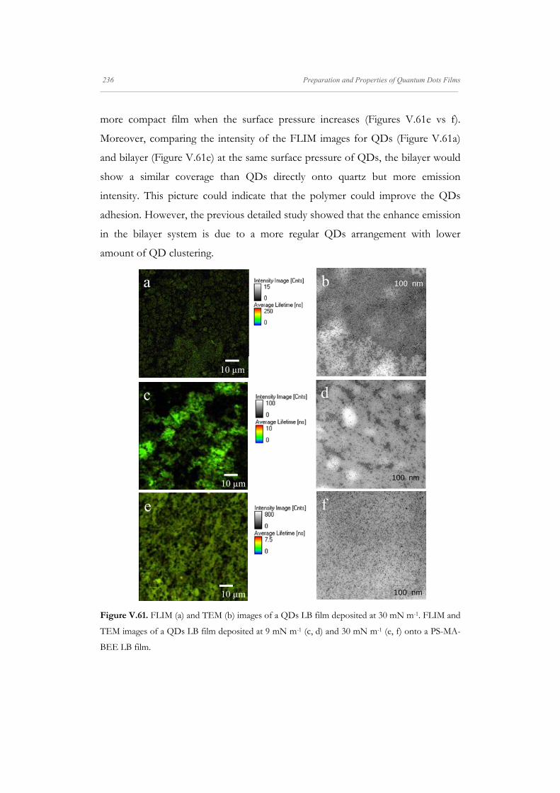
236 Preparation and Properties of Quantum Dots Films _____________________________________________________________________________________________________________________
more compact film when the surface pressure increases (Figures V.61e vs f).
Moreover, comparing the intensity of the FLIM images for QDs (Figure V.61a)
and bilayer (Figure V.61e) at the same surface pressure of QDs, the bilayer would
show a similar coverage than QDs directly onto quartz but more emission
intensity. This picture could indicate that the polymer could improve the QDs
adhesion. However, the previous detailed study showed that the enhance emission
in the bilayer system is due to a more regular QDs arrangement with lower
amount of QD clustering.
Figure V.61. FLIM (a) and TEM (b) images of a QDs LB film deposited at 30 mN m-1. FLIM and
TEM images of a QDs LB film deposited at 9 mN m-1 (c, d) and 30 mN m-1 (e, f) onto a PS-MA-
BEE LB film.
10 µm
10 µm
a
c
10 µm
e
100 nm
f
100 nm
d
100 nmb

Preparation and Properties of Quantum Dots Films 237 _____________________________________________________________________________________________________________________
When we deposit the mixed QD/PS-MA-BEE films, the morphology of
the aggregates observed changes. The AFM images (Figures V.62e, h and j) show
the formation of circular-shape aggregates, whose diameter size decreases when
the polymer mole fraction increases. As in the case of polymer film, the AFM
image in Figure V.62e shows that at XP = 0.50 the quartz physical heterogeneities
can promote the continuous breakup of the film into holes.[368] While the circular
domain formation, observed by AFM for samples above XP > 0.50, is consistent
with the spinodal dewetting mechanism proposed in the case of mica substrate,
see Figures V.62h and j. However, the aggregates formed onto quartz present a
different size, although the AFM roughness (Figures V.62e, h and j) is similar and
close to 3-4 nm, approximately the QDs diameter. A possible explanation for the
formation of circular aggregates with smaller size, Table V.10, could be that as the
quartz is more hydrophobic than mica, cohesive interactions between the film and
the substrate predominate.[369]
Table V.10. Average values of the domains (dots) of QD/PS-MA-BEE mixed LB films deposited
at π = 14 mN m-1 onto mica and quartz substrates obtained from AFM measurements.
Mica Quartz
XP size / μm XP size / μm
0.96 1.10 ± 0.35 0.98 0.07 ± 0.05
0.99 0.52 ± 0.23 0.99 0.18 ± 0.17
*Reported values are averages and error represents the standard deviation determined from at least
25 surface features.
Moreover, the FLIM intensity (counts) indicates that when the polymer
concentration increases the intensity decreases, due to the fact that there are less
quantity of fluorescence material, QDs; and also maybe, the high polymer mole
fraction could affect the QDs luminescence. In fact, the photoluminescence
measurements in solution showed a possible quenching from the polymer due to
aromatic rings, [329] Figure V.37.

238 Preparation and Properties of Quantum Dots Films _____________________________________________________________________________________________________________________
Figure V.62. FLIM, TEM and AFM images of mixed QD/PS-MA-BEE LB films deposited at a
surface pressure of 14 mN m-1 for different polymer mole fractions: 0.35 (a, b); 0.5 (c, d, e); 0.98
(f, g, h); and 0.99 (i, j). The substrate for FLIM and AFM images was polished quartz wafers.
When the surface pressure is increased until 30 mN m-1. The FLIM and
TEM images presented in Figure V.63 show more dense films. It is important to
note that in contrast with low surface coverage, 14 mN m-1 (Figure V.62), at high
surface pressure, 30 mN m-1, the FLIM images brightness is similar when polymer
10 µm
10 µm
10 µm
0 2 4 6 80
4
8
Z /
nm
X / m
0 1 2 30
4
8
Z /
nm
X / m
0 1 20
2
4
Z /
nm
X / m
10 µm
a
c
f
i j
h
e
100 nm
b
100 nm
d
500 nm
g

Preparation and Properties of Quantum Dots Films 239 _____________________________________________________________________________________________________________________
mole fraction increases until exceed 0.65, from Figures V.63a, c and e to Figure
V.63g with XP =0.96.
Figure V.63. FLIM and TEM images of mixed QD/PS-MA-BEE LB films deposited at a surface
pressure of 30 mN m-1 for different polymer mole fractions: 0.35 (a, b); 0.5 (c, d); 0.65 (e, f); and
0.96 (g). The substrate for FLIM images was polished quartz wafers.
100 nm
10 µm
10 µm
10 µm
10 µm
a
c
e
g
d
100 nm
100 nm
f
b

240 Preparation and Properties of Quantum Dots Films _____________________________________________________________________________________________________________________
Finally, in reference to the lifetime scales showed in the FLIM images,
built in fast FLIM mode, they only indicate that the lifetimes are in the same range
order. For a detailed study, it is necessary to modify the measurement conditions,
mainly, laser intensity, repetition rate and channel resolution as was done in the
PL dynamics analysis.
V.4.5.2. QDP/PS-MA-BEE Langmuir-Blodgett Films
In the case of LB films built with the PS-MA-BEE-capped QDs, the
morphologies observed by FLIM are different than in TOPO-capped QDs. On
the one hand, the pure QDP and mixed QDP/PS-MA-BEE (XP =0.50) LB films
show a structure of rafts or blocks, see Figures V.64a and c. However, when the
polymer mole fraction increases in the mixture (Figures V.64d and e) the shape of
aggregates is better defined. As it was previously observed on mica (Figure V.22),
domains are formed (Figure V.64d) by nucleation and growth of holes dewetting
mechanism.[44] These FLIM and TEM images correspond to a mixed film with a
polymer molar fraction of 0.99.

Preparation and Properties of Quantum Dots Films 241 _____________________________________________________________________________________________________________________
Figure V.64. FLIM and TEM images of pure QDP (a, b) and mixed QDP/PS-MA-BEE LB films
deposited at a surface pressure of 14 mN m-1. For the mixed systems the polymer mole fractions
were: 0.5 (c); and 0.99 (d, e). The substrates for FLIM images were polished quartz wafers.
It is relevant to note that the intensity (counts) observed in the samples
with QDP (Figure V.64) is lower than for QDTOPO (Figure V.62). This observation
could be attributed to a loss in the luminescence properties with the ligand
exchange [8] due to a possible loss in the surface passivation (creating traps) and
the effect of polymer aromatic rings as quenchers of CdSe QDs emission [329].
10 µm
10 µm
10 µm
a
c
d
500 nmb
500 nm
e

242 Preparation and Properties of Quantum Dots Films _____________________________________________________________________________________________________________________
Finally, the use of another substrate for the LB deposition has allowed us
to highlight the influence of the physical surface heterogeneities of the substrate
on the film dewetting mechanism.
VI. Chemically Converted Graphene

Chemically converted Graphene 243 _____________________________________________________________________________________________________________________
VI. Chemically converted Graphene
In recent years, graphene has received enormous interest due to its unique
properties, such as high thermal conductivity, great Young modulus and high
intrinsic carrier mobility. More than other materials, graphene exhibits important
fundamental physical phenomena like the anomalous integer quantum Hall effect
at room temperature and the fractional one at low temperatures. Due to its
remarkable properties,[28, 156, 157, 370-372] graphene and its derivatives are promising
candidates for the fabrication of electronic devices,[373] or reinforced filler in
composites and in medicine[27]. However, these unique properties are associated
with monolayer sheets. Therefore, the challenge is to obtain good quality
monolayers of graphene in large quantities.
In this sense, similar to other materials, the success of graphene in
technological applications is related to the availability of production methods for
the synthesis of large quantities of material at low cost. The main challenge in the
production of graphene is the reduction of the aggregation by π-π stacking.
Currently, there are three main routes to produce high-quality graphene flakes:
micromechanical exfoliation,[374] chemical vapour deposition (CVD) of
hydrocarbons on metal substrates,[375] and thermal reduction of silicon carbide[376].
Micromechanical exfoliation gives samples with the highest charge carrier
mobility[377] although the process is time consuming. The other routes require very
high temperatures and/or ultrahigh vacuum, thus that the production of graphene
monolayers at sufficient scale and low cost remains a challenge. The alternative at
these physical methods are the different chemical routes based on the synthesis of
the material. One of them is the longitudinal "unzipping" of carbon nanotubes
route by treatment with KMnO4 [378, 379] that could afford bulk quantities of
graphene nanoribbons whose width depends on carbon nanotubes diameter and
its scalability has yet to be demonstrated[158]. Another alternative and exciting
method is the "total organic synthesis" that proposes the graphene building with

244 Chemically converted Graphene _____________________________________________________________________________________________________________________
benzene-based macromolecules. The major advance in this way is the synthesis of
nanoribbon-like polyacyclic hydrocarbons (PAHs) up to 12 nm in length.[380] The
challenges in this approach are focused on the achievement of dispersibility and
planar morphology for large PAHs and its electronic characterization, thus this
technique could offer a ground-up synthesis of graphene.[29, 156]
Other approach proposed by several authors[29, 381-383] is the graphite liquid-
phase exfoliation in organic solvents (e.g. N,N-dimethylformamide,
tetrahydrofuran, N-methyl-2-pyrrolidone, ethylene glycol) or water but although
the graphene obtained has good quality, its concentration and the percentage of
graphene monolayer in the solution are too low [384]. This process can be assisted
by the addition of surfactants[385, 386] or metal ions such as potassium [387] that act as
intercalation compounds.
Finally, the preparation of graphene based on the chemical oxidation of
graphite followed by a reduction process, is considered one of the most attractive
routes to obtain graphene, because it is a low-cost, versatile for processing and
chemical functionalization and scalable method.[157] However, chemical oxidation
disrupts the electronic structure of graphene by introducing carbonyl, epoxy and
hydroxyl groups in the network.[388] The reduction cannot remove the structural
defects introduced by the oxidation process, and these defects disrupt the band
structure and degrade the electronic properties of graphene. However, it can be
used to prepare conductive and mechanical resistant composite materials,[389]
flexible coatings,[161] gas molecular sensors[390] or even TEM transparent
supports[391].
Furthermore the reduced graphite oxide tends to agglomerate making
further processing difficult. The reduction with the assistance of different
stabilizers [28, 392-394] is an alternative route to obtain good quality graphene sheets.
When the stabilizer is a surfactant such as dodecylbenzene sulphonate,[393] the
surfactant molecule not only plays an important role in controlling the exfoliation

Chemically converted Graphene 245 _____________________________________________________________________________________________________________________
of graphite oxide but also functionalizes the graphene sheets. The functionalized
sheets can be used in several applications such as solar energy storage [29] or Li-ion
batteries[395]. Moreover, non-covalent functionalization of graphene is an
alternative approach to modify the material properties allowing a better processing
and interactions with other compounds without altering the chemical structure of
graphene.[396]
On the other hand, the graphene oxide (GO) or its derivatives are
presented as a promising route with significant economic advantages in the large
scale production of polymer nanocomposites. The polymer/graphene composites
are based on the use of graphene derivatives as nanofillers to improve the
mechanical, electrical, thermal and optic properties.[389, 397] Depending on polymer
type and reducer agent the GO reduction can be carried out in situ or previously,
in order to avoid the polymer reduction. Moreover, if the chemically converted
graphene has functional groups that are reactive with the polymer, interfacial
interactions between polymer and RGO sheet surface can occur obtaining water-
dispersible graphene.[398] The adhesion between graphene and polymers is also an
important factor to be considered in designing composite materials. Thus, if thin
layers of electrically conductive graphene can be deposited on polymer surfaces,
flexible displays, thin-film transistors and photovoltaic devices will be made
possible.[389]
In this chapter, we present the results corresponding to the study of the
effect of the zwitterionic surfactant dodecyl dimethyl ammonium propane
sulphonate (DDPS) on the quality of the reduced graphite oxide (RGO). The
advantage of this approach is that the zwitterionic surfactants exhibit greater
adsorption onto hydrophobic surfaces such as graphite than the ionic
surfactants,[399, 400] therefore, we expect that the functionalization of RGO with
DDPS provides better quality of the RGO sheets than that obtained with ionic
surfactants. On the other hand, the charged groups of DDPS molecules attached

246 Chemically converted Graphene _____________________________________________________________________________________________________________________
on RGO can bind metal cations[29] and different kind of polymers[282, 401-402]
producing nanocomposites with potential applications in the construction of
photovoltaic devices[29] and sensors,[30] respectively. Moreover, the zwitterionic
surfactants present higher tolerance to extreme pH, strong electrolytes, and
oxidizing and reducing agents than the ionic ones,[399] therefore they have utility in
the fabrication of devices subjected to extreme conditions.
To evaluate the quality of the reduced sheets we use the criteria proposed
by Luo et al.[403] These criteria consist in analyzing simultaneously the reduction
degree, the defect repair degree and the electric conductivity of the obtained
graphitic material by using AFM, X-Ray photoelectron spectroscopy (XPS), UV-
vis absorption spectroscopy, Micro-Raman spectroscopy and electric conductivity
measurements. We are also interested in exploring the effect of the reducer agent
on the quality of the reduced graphite oxide flakes and on the functionalization
process of the RGO. With this objective in mind we have selected two reducer
agents, hydrazine and Vitamin C. Hydrazine is one of the most widely used
reducer agents of GO and renders good quality RGO sheets [403] while Vitamin C
has been proposed as substitute for hydrazine as non-toxic reagent. Previous
results have demonstrated that Vitamin C is a good reducer agent of GO and
renders flakes with less structural defects than hydrazine,[404-408] but a simultaneous
analysis of the reduction and defect repair degrees and electric conductivity has
not yet been done. Therefore, we analyze the quality of the RGO obtained by
reduction with Vitamin C using the Luo's criteria [403] not only the sp2 character of
the RGO. In addition, we have analyzed the effect of the reducer agents on the
functionalization of the RGO samples by the surfactant DDPS. To the best of
our knowledge, it is the first time that the effect of the reducer agent on the
functionalization of RGO sheets has been studied.
On the other hand, the implementation of graphene obtained by chemical
reduction of GO into device fabrication processes requires an uniform and

Chemically converted Graphene 247 _____________________________________________________________________________________________________________________
reproducible deposition methodology. Several techniques such as drop-casting[162]
or spin-coating[162, 163] have been used to obtain graphene films onto solid wafers.
However, these methodologies often result in non-uniform film thickness on
solid substrates.[156] An effective method to obtain well defined sheets deposited
onto solid wafer can be the Langmuir-Blodgett (LB) technique. This methodology
has been successfully used to transfer water-insoluble molecules[3, 111] or
nanomaterials[304, 409] from the air-water interface onto solids and presents several
advantages since it allows a great control of the interparticle distance and,
consequently, of the interparticle interactions. Recently this technique has been
used for deposition of graphene oxide[76] and multilayered films of graphene
sheets[75]. Therefore, we use the LB methodology to deposit no collapsed sheets of
the different RGO samples. The morphology and quality of the LB deposited
sheets were studied by means of atomic force microscopy (AFM), field emission
scanning electron microscopy (FE-SEM) and Micro-Raman spectroscopy.
VI.1. Oxidation and Reduction Procedures of Graphitic Material
In order to set the approaches selected, a run-through of the main existent
methodologies for graphene oxide production and its reduction are presented.
VI.1.1. Graphite Oxide Production
The first approach for the graphite oxide (GO) obtaining was developed
by B.C. Brodie in 1859. The reaction performed was based on the addition of
potassium chlorate (KClO3) to a slurry of graphite flakes in fuming nitric acid
(HNO3).[410] Nearly 40 years after, L. Staudenmaier improved Brodie's KClO3-
fuming HNO3 preparation by adding the chlorate in multiple aliquots over the
course of the reaction and also, with the addition of concentrated sulfuric acid, to
increase the acidity of the mixture, rather than in a single addition as in the
Brodie's method. This slight change in the procedure resulted in an overall extent
of oxidation similar to Brodie's multiple oxidation approach, but performed more
practically in a single reaction vessel.[411] In this procedure, nitric acid reacts

248 Chemically converted Graphene _____________________________________________________________________________________________________________________
strongly with aromatic carbon surfaces resulting in the formation of various
oxide-containing species including carboxyls, lactones and ketones with the
liberation of gaseous NO2 and/or N2O4 and ClO2. Likewise, potassium chlorate is
a strong oxidizing agent and an in situ source of oxygen, which acts as the reactive
species.[412]
Later, in 1958, Hummers and Offeman developed an alternative oxidation
method by reacting graphite with a mixture of potassium permanganate (KMnO4),
sodium nitrate (NaNO3) and concentrated sulfuric acid (H2SO4), achieving similar
levels of oxidation.[413] In this case, although permanganate is an oxidant, the
active species is, in fact, diamanganese heptoxide formed from the reaction of
potassium permanganate with sulfuric acid. The bimetallic heptoxide is far more
reactive than its monometallic tetraoxide counterpart, and is known to detonate
when heated to temperatures greater than 55 ºC or when placed in contact with
organic compounds, therefore, the mixture is carried out over an ice-bath.[414-415]
Though others have developed slightly modified versions in the last
decade, these three methods comprise the primary routes for obtaining GO, and
little about them has changed. Importantly, it has since been demonstrated that
the products of these reactions show strong variance, depending not only on the
particular oxidants used, but also on the graphite source and reaction conditions.
In fact, the slight modifications proposed are based on the change of the reactive
quantities or ratios, reaction times and the sum of pre-oxidation stages (e.g. a
graphite treatment with H2SO4/K2S2O8/P2O5)[416] in order to obtain a carbon
material more oxidized. Several efforts have been carried out in this line in these
recent years. One of these modifications is the use of KMnO4 and a 9:1 mixture
of concentrated H2SO4/H3PO4 avoiding the NaNO3 addition, whose advantages
are that the protocol for running the reaction does not involve a large exothermal
step, produces no toxic gas (NO2 and/or N2O4) and yields a higher fraction of
well-oxidized hydrophilic carbon material.[417]
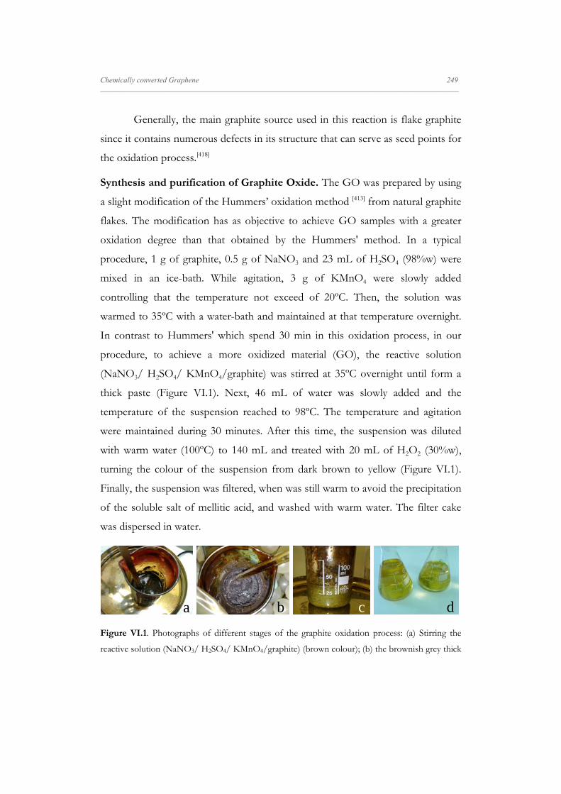
Chemically converted Graphene 249 _____________________________________________________________________________________________________________________
Generally, the main graphite source used in this reaction is flake graphite
since it contains numerous defects in its structure that can serve as seed points for
the oxidation process.[418]
Synthesis and purification of Graphite Oxide. The GO was prepared by using
a slight modification of the Hummers’ oxidation method [413] from natural graphite
flakes. The modification has as objective to achieve GO samples with a greater
oxidation degree than that obtained by the Hummers' method. In a typical
procedure, 1 g of graphite, 0.5 g of NaNO3 and 23 mL of H2SO4 (98%w) were
mixed in an ice-bath. While agitation, 3 g of KMnO4 were slowly added
controlling that the temperature not exceed of 20ºC. Then, the solution was
warmed to 35ºC with a water-bath and maintained at that temperature overnight.
In contrast to Hummers' which spend 30 min in this oxidation process, in our
procedure, to achieve a more oxidized material (GO), the reactive solution
(NaNO3/ H2SO4/ KMnO4/graphite) was stirred at 35ºC overnight until form a
thick paste (Figure VI.1). Next, 46 mL of water was slowly added and the
temperature of the suspension reached to 98ºC. The temperature and agitation
were maintained during 30 minutes. After this time, the suspension was diluted
with warm water (100ºC) to 140 mL and treated with 20 mL of H2O2 (30%w),
turning the colour of the suspension from dark brown to yellow (Figure VI.1).
Finally, the suspension was filtered, when was still warm to avoid the precipitation
of the soluble salt of mellitic acid, and washed with warm water. The filter cake
was dispersed in water.
Figure VI.1. Photographs of different stages of the graphite oxidation process: (a) Stirring the
reactive solution (NaNO3/ H2SO4/ KMnO4/graphite) (brown colour); (b) the brownish grey thick
a b c d

250 Chemically converted Graphene _____________________________________________________________________________________________________________________
paste oxidized after overnight; (c) addition of H2O2 turning the solution to yellow; and (d) the GO
obtained after the purification step.
In order to obtain high quality GO we use a centrifugation-based
purification procedure published elsewhere.[76] Thus, the GO filter cake was
dispersed in water by mechanical agitation, and centrifugated at 1000 rpm (90g)
for 3-5 times, allowing to remove the biggest (visible) particles. The supernatant
was treated with high-speed centrifugation at 5000 rpm (3750g) for 15 min, in
order to eliminate the small GO particles and the water-soluble products of the
oxidation process. Finally, the supernatant was centrifuged at 10000 rpm (8163g)
for 15 min to separate the GO sediment, which was then dried at 40 ºC over
phosphorus pentoxide in vacuum.[413]
The GO samples were characterized by X-ray photoelectron spectroscopy
(XPS) and the results are reported in Table VI.1. The C1s core-level spectrum of
GO was fitted by three components centred at 284.8, 286.3 and 288.6 eV, being
the first two more intense than the third one (Figure VI.2a, Table VI.1). These
peaks are assigned to C-C bonds in aromatic networks, to C-O bonds in alcohols
or epoxy groups and to COO- structures, respectively. In addition, the O1s core-
level spectrum shows two peaks at 531.4 and 533.6 eV (Figure VI.2b). The first
one is assigned to oxygen in C=O groups while the later comes from C-O bonds
and it is more intense than the first one. This observation indicates that the epoxy
and hydroxyl groups are the major components, in agreement with results
previously obtained.[419]

Chemically converted Graphene 251 _____________________________________________________________________________________________________________________
Figure VI.2. The C1s (a) and O1s (b) core-level spectra of graphite oxide (GO).
The O/C ratio value calculated from XPS was 0.62. This value is higher
than the values found in the literature comprised between 0.37 and 0.53.[165, 392, 405-
407] This fact confirms that the method used in this work allows us to obtain a
more oxidized material (GO) than those reported by other oxidation procedures.
526 528 530 532 534 536 538280 284 288 292
C-O533.6 eV
C=O531.4 eV
Binding Energy / eV
b
C
ount
s pe
r se
cond
/ a.
u.
Binding Energy / eV
C-C sp2
C-O
O-C=O
a

252 Chemically converted Graphene _____________________________________________________________________________________________________________________
Table VI.1. Binding energies (eV) and O/C, N/C and S/C surface atomic ratios of graphitic
samples.
Sample C1s S2p N1s O/C N/C S/C
GO
284.8 (49 ± 2)
286.9 (45 ± 2)
288.6 (6 ± 0.5)
- - 0.618 - -
RGO Hydrazine
284.8 (63 ± 2)
286.3 (22 ± 2)
287.7 (8 ± 1)
289.3 (7 ± 0.5)
- 400.0 0.119 0.039 -
RGO Hydrazine
(DDPS)
284.8 (82 ± 1)
286.3 (16 ± 0.5)
289.0 (2 ± 0.5)
167.8 399.8 (60 ± 1)
401.9 (40 ± 1)0.190 0.004 0.002
RGO Vitamin C
284.8 (67 ± 1)
286.4(29 ± 0.4 )
288.9 (4 ± 0.2)
- - 0.339 - -
RGO Vitamin C (DDPS)
284.8 (77 ± 6)
286.2 (20 ± 3)
289.0 (3 ± 0.5)
168.6 402.2 0.209 0.006 0.006
DDPS 284.8 (82)
286.2 (18) 167.5 402.3 0.183 0.056 0.056
VI.1.2. Reduction of Graphite Oxide
As it was mentioned, the GO is an electrically insulating material due to its
disrupted sp2 bonding network, thus, the next step is its reduction to partially
restore the network and therefore its electrical conductivity. The reduction can be
achieved through chemical, thermal or electrochemical reduction pathways. In our
case, the reduction was carried out by chemical reaction of GO with hydrazine
and Vitamin C.
Chemical Reduction. There are several reducer agents proposed to carry out the
chemical reduction of GO. However, the most common used is the hydrazine

Chemically converted Graphene 253 _____________________________________________________________________________________________________________________
monohydrate (N2H4).
[165] While most strong reducers have slight to very strong
reactivity with water, hydrazine monohydrate does not, making it an attractive
option for reducing aqueous dispersions of GO. Although the mechanism of this
reaction remains unclear, several mechanistic routes have been proposed. In all
these routes, the hydrazine mainly attacks the epoxide groups forming diazene
and in some points introducing residual nitrogen functionality on the carbon
network.[165, 420] The de-epoxidation occurs in three steps: in the first, hydrazine
(N2H4) attacks the carbon of epoxide from the back side of the epoxide ring
opening the ring. Second, the C-C bond of the intermediate 1 rotates to bring the
hydrazine group (-H2NNH2) attached to the opposite side of the oxygen close to
the oxygen. Then one H-atom transfers from the hydrazine group to the oxygen
of epoxide, forming a hydrazino alcohol intermediate 2. Third, another H of
intermediate 2 transfers from the hydrazino group (-HNNH2) to the hydroxyl
group (-OH). This gives a water molecule (H2O), a cis-diazene (cis-N2H2), and the
deoxygenated product.
O
O
H2O-
GO RGO
H2N NH2HN NH
N N
HH
HH
OH
N N
H
HH
+
O
NN
H
H H
H HO
N N
HH
H H2O-
RGO
HN NH+
O
NN
H
H H
H H2O-HO
N N
HH
H NN H
H
O
N
N
HH
HO
H
H
N
N
H
H
H
H2O-
RGO
HN NH+
Intermediate 1 Intermediate 2
Scheme VI.1. Proposed reduction mechanism of GO by hydrazine (Adapted from Gao, 2009[420]).
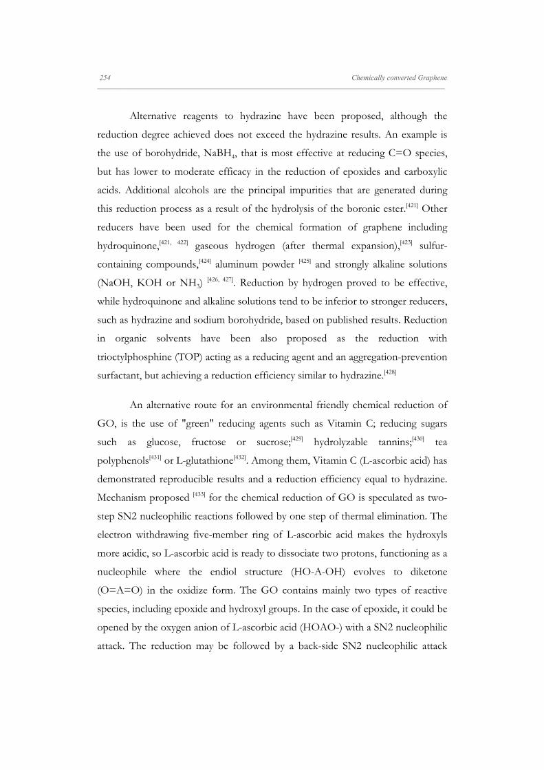
254 Chemically converted Graphene _____________________________________________________________________________________________________________________
Alternative reagents to hydrazine have been proposed, although the
reduction degree achieved does not exceed the hydrazine results. An example is
the use of borohydride, NaBH4, that is most effective at reducing C=O species,
but has lower to moderate efficacy in the reduction of epoxides and carboxylic
acids. Additional alcohols are the principal impurities that are generated during
this reduction process as a result of the hydrolysis of the boronic ester.[421] Other
reducers have been used for the chemical formation of graphene including
hydroquinone,[421, 422] gaseous hydrogen (after thermal expansion),[423] sulfur-
containing compounds,[424] aluminum powder [425] and strongly alkaline solutions
(NaOH, KOH or NH3) [426, 427]. Reduction by hydrogen proved to be effective,
while hydroquinone and alkaline solutions tend to be inferior to stronger reducers,
such as hydrazine and sodium borohydride, based on published results. Reduction
in organic solvents have been also proposed as the reduction with
trioctylphosphine (TOP) acting as a reducing agent and an aggregation-prevention
surfactant, but achieving a reduction efficiency similar to hydrazine.[428]
An alternative route for an environmental friendly chemical reduction of
GO, is the use of "green" reducing agents such as Vitamin C; reducing sugars
such as glucose, fructose or sucrose;[429] hydrolyzable tannins;[430] tea
polyphenols[431] or L-glutathione[432]. Among them, Vitamin C (L-ascorbic acid) has
demonstrated reproducible results and a reduction efficiency equal to hydrazine.
Mechanism proposed [433] for the chemical reduction of GO is speculated as two-
step SN2 nucleophilic reactions followed by one step of thermal elimination. The
electron withdrawing five-member ring of L-ascorbic acid makes the hydroxyls
more acidic, so L-ascorbic acid is ready to dissociate two protons, functioning as a
nucleophile where the endiol structure (HO-A-OH) evolves to diketone
(O=A=O) in the oxidize form. The GO contains mainly two types of reactive
species, including epoxide and hydroxyl groups. In the case of epoxide, it could be
opened by the oxygen anion of L-ascorbic acid (HOAO-) with a SN2 nucleophilic
attack. The reduction may be followed by a back-side SN2 nucleophilic attack
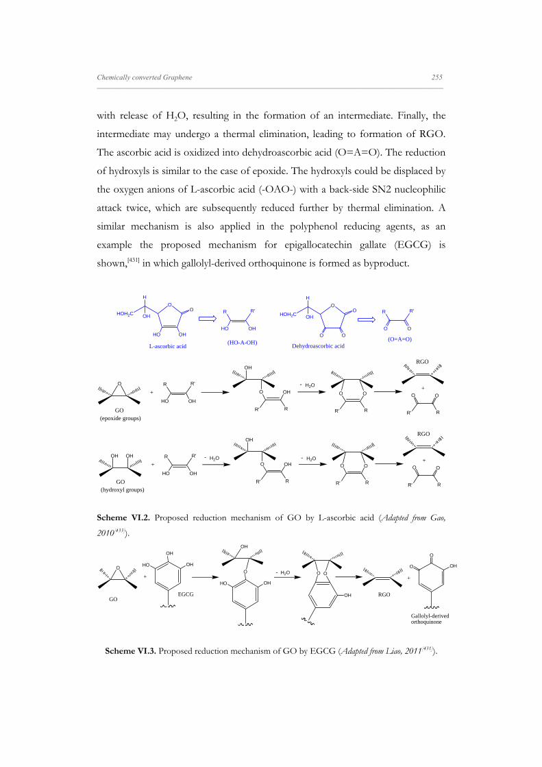
Chemically converted Graphene 255 _____________________________________________________________________________________________________________________
with release of H2O, resulting in the formation of an intermediate. Finally, the
intermediate may undergo a thermal elimination, leading to formation of RGO.
The ascorbic acid is oxidized into dehydroascorbic acid (O=A=O). The reduction
of hydroxyls is similar to the case of epoxide. The hydroxyls could be displaced by
the oxygen anions of L-ascorbic acid (-OAO-) with a back-side SN2 nucleophilic
attack twice, which are subsequently reduced further by thermal elimination. A
similar mechanism is also applied in the polyphenol reducing agents, as an
example the proposed mechanism for epigallocatechin gallate (EGCG) is
shown,[431] in which gallolyl-derived orthoquinone is formed as byproduct.
H2O
GO
RGO
O
OHHO
OHOH2C
H
OH
O
OO
OHOH2C
H
OH
HO OH
R R'
(HO-A-OH)(O=A=O)
O O
R R'
Dehydroascorbic acidL-ascorbic acid
O
HO OH
R R'
+
OH
OHO
RR'
-
OO
RR'
+OO
RR'
H2O
GO
RGO
OH
HO OH
R R'
+
OH
OHO
RR'
-
OO
RR'
+OO
RR'
OH H2O-
(epoxide groups)
(hydroxyl groups)
Scheme VI.2. Proposed reduction mechanism of GO by L-ascorbic acid (Adapted from Gao,
2010[433]).
O
+
OH
OHHO
OH
O
OHHO
O
OH
O+
O
OHOH2O-
GOEGCG RGO
Gallolyl-derived orthoquinone
Scheme VI.3. Proposed reduction mechanism of GO by EGCG (Adapted from Liao, 2011[431]).

256 Chemically converted Graphene _____________________________________________________________________________________________________________________
Alternative approaches to chemical reduction are the thermal and the
electrochemical reduction. The thermally-mediated reduction employs an
annealing step where the oxide functionality from the surface is stripped by
directly heating GO in a furnace at temperatures between 150-1100 ºC. This step
can be performed with other reduction approaches as a last stage in order to
improve the reduction efficiency and the quality of the RGO structure.[427] Several
approaches combine high temperatures with an atmosphere of Ar/H2 [420] or even
with an acetylene-assisted reduction, using this compound as a supplemental
carbon source to repair substantial defects within GO sheets [434]. The last method
for the reduction of GO relies on the electrochemical removal of the oxygen
functionalities. Firstly thin films of GO are deposited onto a substrate. After
deposition on a variety of substrates such as glass, plastic, ITO, etc., electrodes
were placed at opposite ends of the film and linear sweep voltammetry was run in
a sodium phosphate buffer. Reduction began at -0.60 V and reached a maximum
at -0.87 V. Rapid reduction was observed during the first 300 s, followed by a
reduced rate of reduction up to 2000 s, and finally a decrease to background
current levels up to 5000 s. A priori this method could avoid the use of dangerous
reducers (e.g. hydrazine) and the need to dispose of the by-products.[435]
Focusing on the chemical reduction of the GO obtained, we perform two
different routes: a chemical route and a chemical-colloidal route (Figure VI.3). In
the first one, we use the following reducer agents: hydrazine and Vitamin C in
aqueous solution. On the other, we add a surfactant, DDPS, in the GO reaction
medium before the reduction step in order to improve the exfoliation stage. The
reduction was carried out with the same reducer agents.

Chemically converted Graphene 257 _____________________________________________________________________________________________________________________
Figure VI.3. Photographs of aqueous dispersions of the starting material, GO, (1) and RGO
obtained by reduction with: hydrazine (2); hydrazine with DDPS surfactant (3); Vitamin C (4) and
Vitamin C with DDPS surfactant (5).
VI.1.2.1. Chemical Reduction of GO with Hydrazine
The GO (1 mg mL-1, sonication 1 h) was reduced with hydrazine in water
by the Stankovich’s method.[165] The hydrazine ratio was 0.02 mL per 1 mg GO
and the reaction was maintained at 100ºC during 24 h. The reduced product was
filtered and washed with water and methanol. It is important to note that the
reduced dispersion is only stable a few weeks, after which, the RGO sheets
precipitated.
For comparative purposes, the GO reduction was also carried out by
exposure of GO LB deposited sheets to hydrazine vapour (0.1 mL) during 18 h at
room temperature [76] in a closed homemade container. To deposit the GO sheets
by LB method, we prepared the GO Langmuir monolayer by spreading the GO
dispersion in MeOH:H2O (5:1 v/v, sonication 30 min) on the air-water
interface.[76] The GO sheets were transferred by symmetric barrier compression
(50 mm min-1) with the substrate into the trough by vertically dipping it up at 2
mm min-1 and then it was reduced by hydrazine vapour and later rinsed with water
and dried in an oven for 1 h (80ºC).
1 2 3 4 5

258 Chemically converted Graphene _____________________________________________________________________________________________________________________
VI.1.2.2. Chemical Reduction of GO with Vitamin C
To reduce the GO with Vitamin C, the pH of the GO aqueous
dispersions (0.1 mg mL-1, sonication time 1 h) was adjusted to 9-10 with an
ammonia solution of 25% and then, the reducer agent, Vitamin C (2 mM) was
added. The reactive solution was heated at 95ºC during 15 min.[405] The reduced
dispersion was processed by filtration with a PVDF membrane (0.2 µm pore size)
supplied by Filter-lab.
In this case, the reduction aqueous dispersion formed by the RGO
samples obtained from GO reduced by Vitamin C was stable during several
months.
VI.1.2.3. Chemical Reduction of GO assisted by the Surfactant DDPS
The chemical reduction was carried out in the presence of the DDPS
surfactant by using GO dispersed in surfactant solutions and the reduction
procedures previously described. Thus, the concentration of the reducers,
hydrazine and Vitamin C, and their respective reaction conditions (temperature
and time) were kept.
To form the GO/surfactant dispersion, first we prepared a stable water
dispersion of GO (0.5 mg mL-1) by ultrasonic treatment (1 h) exfoliating the GO.
Next, the surfactant was added and the dispersion was mechanically stirred during
2 h and finally again sonicated (1 h). In order to optimize the reduction of GO,
the DDPS concentration was modified above and below the CMC (1.1 mg mL-1) [174]. Surfactant concentrations below the CMC did not give stable dispersions, in
contrast surfactant solutions with concentrations above 2 mg mL-1 gave rise to
small precipitates after a few days. Therefore, we keep the surfactant
concentration in 1.7 mg mL-1 which is twice the CMC of DDPS and form stable
and clear GO dispersions during a few weeks. This result indicates that the
optimum surfactant concentration value required to stabilize the GO dispersion is
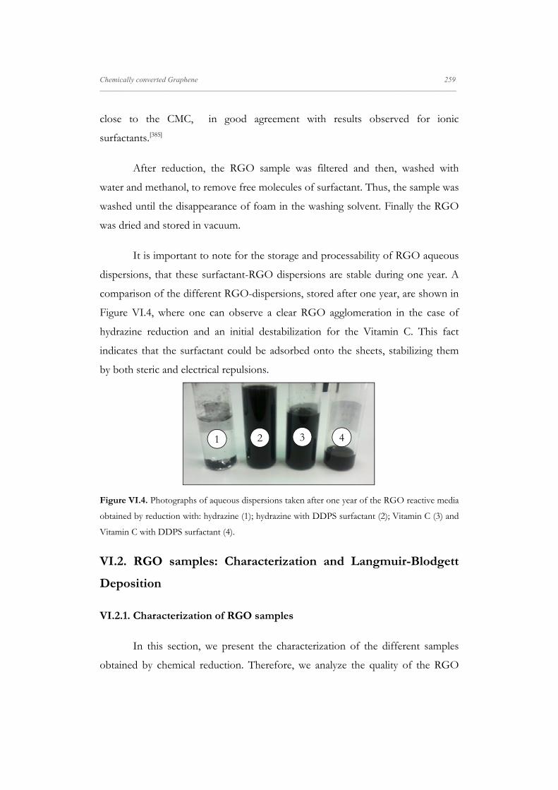
Chemically converted Graphene 259 _____________________________________________________________________________________________________________________
close to the CMC, in good agreement with results observed for ionic
surfactants.[385]
After reduction, the RGO sample was filtered and then, washed with
water and methanol, to remove free molecules of surfactant. Thus, the sample was
washed until the disappearance of foam in the washing solvent. Finally the RGO
was dried and stored in vacuum.
It is important to note for the storage and processability of RGO aqueous
dispersions, that these surfactant-RGO dispersions are stable during one year. A
comparison of the different RGO-dispersions, stored after one year, are shown in
Figure VI.4, where one can observe a clear RGO agglomeration in the case of
hydrazine reduction and an initial destabilization for the Vitamin C. This fact
indicates that the surfactant could be adsorbed onto the sheets, stabilizing them
by both steric and electrical repulsions.
Figure VI.4. Photographs of aqueous dispersions taken after one year of the RGO reactive media
obtained by reduction with: hydrazine (1); hydrazine with DDPS surfactant (2); Vitamin C (3) and
Vitamin C with DDPS surfactant (4).
VI.2. RGO samples: Characterization and Langmuir-Blodgett
Deposition
VI.2.1. Characterization of RGO samples
In this section, we present the characterization of the different samples
obtained by chemical reduction. Therefore, we analyze the quality of the RGO
1 2 3 4

260 Chemically converted Graphene _____________________________________________________________________________________________________________________
flakes by means of UV-vis and XPS measurements previous to the RGO
deposition.
We evaluate the efficiency of the reducer agents by analyzing the position
of the maximum of the UV-vis absorption spectra of the different samples
(Figure VI.5). The maximum position values of the UV-vis spectra are reported in
Table VI.2. For GO, one can see that the position of the maximum is centred at
230 nm, in agreement with the literature values.[75] After reduction, the absorption
peak red shifts to 264 nm and 265 nm for reduction with hydrazine and Vitamin
C, respectively. It is known that the GO reduction causes a red shift in the
absorption maximum,[75] so that our observations indicate that both the Vitamin C
and hydrazine are good reducer agents of GO and that reduction achieved is
similar for the two reducer agents.
200 400 600 8000.0
0.2
0.4
0.6
0.8
1.0
Abs
orba
nce
/ a.u
.
/ nm
GO
d
c
b
a
Figure VI.5. UV-vis absorption spectra of aqueous dispersions of the starting material, GO, and
RGO obtained by reduction with: hydrazine (a); hydrazine with DDPS surfactant (b); Vitamin C
(c) and Vitamin C with DDPS surfactant (d).

Chemically converted Graphene 261 _____________________________________________________________________________________________________________________
As the position of the maximum of the UV-vis spectra is a qualitative
indicator, the X-Ray photoelectron spectroscopy (XPS) was employed to analyze
the reduction degree of the RGO samples in a quantitative way.
Table VI.2. UV-vis absorption peak position for aqueous GO solutions and different RGO
samples dissolved in chloroform. The concentration was kept constant in 0.1 mg mL-1. Percentage
of C (sp2) and the Raman intensity ratio values found for different graphitic samples. Electric
conductivity values of the different RGO paper-like films.
Figure VI.6a displays the C1s core-level spectra of different samples. The
asymmetric peak of the C1s was fitted to three or four components centred at
284.8 eV (aromatic sp2), 286.9 eV (C-O), 287.7 eV (C=O) and 290 eV (O-C=O),
respectively.[392] Results obtained for the different samples are summarized in
Table VI.1. Each reported value is the average over at least three spectra, and the
standard deviation of these measurements was considered the experimental error.
From data reported in Table VI.1 and Figure VI.6a, it can be seen that the most
significant change after the GO reduction is the increase of the sp2 component,
indicating an increase of the proportion of reduced carbons upon the reduction.
The value of the sp2 component found for RGO reduced by hydrazine is in good
agreement with those obtained by other authors.[403, 433, 436] Our results also show
similar sp2 component for samples reduced by hydrazine and Vitamin C, in good
agreement with results in the literature.[405] Moreover, results in Table VI.2 indicate
Sample λ max / nm % C (sp2) ID/IG Conductivity / S m-1 Graphite Oxide 230 ± 2 49 ± 1 1.42 insulator
RGO Hydrazine
264 ± 2 63 ± 2 --- 241 ± 29
RGO Hydrazine vapour
--- --- 1.99 ---
RGO Hydrazine
(DDPS) 268 ± 2 82 ± 1 1.45 484 ± 58
RGO Vitamin C
265 ± 2 67 ± 1 0.67 37 ± 4
RGO Vitamin C (DDPS)
266 ± 2 77 ± 6 0.92 580 ± 70

262 Chemically converted Graphene _____________________________________________________________________________________________________________________
that the O/C atomic ratio of RGO sample reduced by Vitamin C is higher than
for the sample reduced by hydrazine, Table VI.1. The increase of the O/C ratio
can be due to the formation of hydrogen bonds between the oxidized product of
Vitamin C and the residual oxygen on the RGO.[406]
Figure VI.6. (a) The C1s core-level spectra of graphite oxide (GO), and RGO samples reduced
with: hydrazine; hydrazine dissolved in DDPS; Vitamin C and Vitamin C dissolved in DDPS
solutions. (b) The N1s core-level spectra of dodecyl dimethyl ammonium propane sulphonate
(DDPS) and RGO samples reduced with: Vitamin C dissolved in DDPS solutions, hydrazine
dissolved in DDPS solutions and hydrazine.
We also recorded the N1s core-level spectra of different chemically
reduced graphite samples. Figure VI.6b shows the spectra of these samples. It is
interesting to note that the N1s for RGO reduced with hydrazine presents one
peak centred at 400 eV while no N1s peak was detected for the RGO reduced by
Vitamin C. It is well documented that the reduction of the epoxy groups at the
edges of the GO network using hydrazine is blocked by the formation of the
hydrazino alcohol,[433] so that the XPS peak at 400 eV can be ascribed to the
280 285 290 295
C-C sp2
C-O
O-C=O
GO
Hydrazine (DDPS)
O-C=O
C-C sp2
C-O
C = O
Hydrazine
C-C sp2
C-O
O-C=O
Vitamin C
Binding Energy / eV
Vitamin C (DDPS)
Cou
nts
per
sec
ond
/ a.
u.
C-C sp2
C-OO-C=O
C-C sp2
C-OO-C=O
Vitamin C (DDPS)
392 396 400 404 408
Hydrazine (DDPS)
Cou
nts
per
sec
ond
/ a.
u.
DDPS
Hydrazine
N-H
Binding Energy / eV
a b

Chemically converted Graphene 263 _____________________________________________________________________________________________________________________
nitrogen atoms (R2N
-, amine nitrogen) attached to the RGO sheets,[437] as shown
scheme VI.4.
RGOO
NN
H
H H
H H2O-HO
N N
HH
H NN H
H
Scheme VI.4. One of the possible steps in the reduction mechanism of GO with hydrazine that
results in the attachment of nitrogen atoms to the RGO sheets.
On the other hand, we also analyzed the efficiency of the reduction
process for the two reducer agents dissolved in surfactant solutions by analyzing
both, the UV-absorption spectrum and the C1s core-level spectra, Table VI.2 and
Figure VI.6a, respectively. As can be seen, using these reducer agents the peak
positions of the UV-vis absorption spectra are also red shifted respect to the
spectrum of GO (Table VI.2) indicating that a good reduction is achieved in the
presence of the surfactant. Moreover, by comparing with the spectra of RGO
samples obtained without surfactant, the red shift is greater, indicating that the
surfactant seems to improve the reduction efficiency. To confirm this picture the
XPS spectra of these samples were recorded. The C1s core-level spectra, Figure
VI.6a, are decomposed into three peaks centred at 284.8 eV (aromatic sp2), 286.9
eV (C-O), and 290 eV (O-C=O), respectively.[392] When we compare the
percentage of Csp2 for RGO samples reduced in the absence of surfactant with
those obtained in the presence of surfactant molecules (Tables VI.1 and 2) we can
conclude that the surfactant improves the reduction of the GO. This fact can be
due to the exfoliation effect carried out by the surfactant molecules attached to
the GO network.

264 Chemically converted Graphene _____________________________________________________________________________________________________________________
To corroborate the functionalization of the RGO flakes by the surfactant
DDPS we recorded the XPS spectra of the different samples. Figure VI.6b
presents the N1s core-level spectra of the samples. As can be seen in the Figure
VI.6b the RGO samples prepared in surfactant solutions present two peaks
centred at 402 eV and 168 eV. In order to assign these peaks we compare these
spectra with the XPS spectrum of the surfactant DDPS. For comparison Figure
VI.6b presents the surfactant DDPS spectrum among the RGO spectra. The N1s
core-level spectrum of the DDPS surfactant shows a symmetric peak centred at a
binding energy of 402.3 eV which is similar to that recorded for RGO samples
reduced in the presence of DDPS surfactant (see Figure VI.6b and Table VI.1).
The XPS spectrum of the surfactant also presents the S2p core-level spectrum of
the sulphonate group at the binding energy of 167.5 eV.[392] The small shift in the
binding energy of S2p peak in RGO samples with respect to the surfactant one
reflects the zwitterionic nature of the surfactant. From these results we can
conclude that the synthesis proposed in this work allows obtaining RGO flakes
with surfactant molecules attached to the graphitic network, i.e., functionalized
RGO.
It is also interesting to note that when the reduction is carried out with
hydrazine assisted by the surfactant DDPS, the N1s core-level spectrum consists
of an asymmetric band that can be decomposed into two peaks centred at 399.8
eV and 402.0 eV, respectively. As commented above, the peak centred at 402 eV
was ascribed to the nitrogen atoms of the surfactant attached to the RGO
sheets,[437] while the peak at 399.8 eV is due to the nitrogen atoms attached to the
RGO reduced with hydrazine, and it appears in the spectrum of RGO samples
reduced with hydrazine as was mentioned. From our results we can conclude that
the surfactant cannot completely inhibit the defects introduced by nitrogen groups
attached to the network, however, improves the quality of the RGO flakes
decreasing the N/C atomic ratio from 0.039 for hydrazine to 0.004 for hydrazine
dissolved in DDPS.
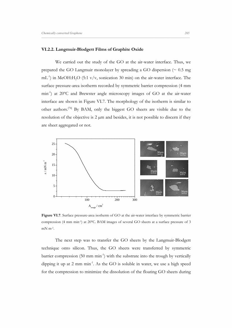
Chemically converted Graphene 265 _____________________________________________________________________________________________________________________
VI.2.2. Langmuir-Blodgett Films of Graphite Oxide
We carried out the study of the GO at the air-water interface. Thus, we
prepared the GO Langmuir monolayer by spreading a GO dispersion (~ 0.5 mg
mL-1) in MeOH:H2O (5:1 v/v, sonication 30 min) on the air-water interface. The
surface pressure-area isotherm recorded by symmetric barrier compression (4 mm
min-1) at 20ºC and Brewster angle microscopy images of GO at the air-water
interface are shown in Figure VI.7. The morphology of the isotherm is similar to
other authors.[76] By BAM, only the biggest GO sheets are visible due to the
resolution of the objective is 2 µm and besides, it is not possible to discern if they
are sheet aggregated or not.
Figure VI.7. Surface pressure-area isotherm of GO at the air-water interface by symmetric barrier
compression (4 mm min-1) at 20ºC. BAM images of several GO sheets at a surface pressure of 3
mN m-1.
The next step was to transfer the GO sheets by the Langmuir-Blodgett
technique onto silicon. Thus, the GO sheets were transferred by symmetric
barrier compression (50 mm min-1) with the substrate into the trough by vertically
dipping it up at 2 mm min-1. As the GO is soluble in water, we use a high speed
for the compression to minimize the dissolution of the floating GO sheets during
100 200 3000
5
10
15
20
25
/ m
N m
-1
Atrough
/ cm2
30µm 30µm
30µm
30µm
30µm
30µm
266 Chemically converted Graphene _____________________________________________________________________________________________________________________
the deposition process. In fact, during the formation of the monolayer, it is
possible to observe how the water subphase slightly changes its colour to
yellowish brown. Really, the monolayer situation is between a Langmuir (floating
sheets) and a Gibbs (soluble sheets) film. Besides, we selected the surface pressure
of 3 mN m-1 in order to obtain no overlapped sheets to a better individual later
characterization of sheets by FE-SEM, AFM and Raman. Figure VI.8a shows the
FE-SEM image of the GO sheets deposited on silicon. The AFM profiles of GO
sheets show a height of ~ 1.7 nm compatible with a bilayer of graphite oxide
(Figure VI.8b).
The Raman spectrum (Figure VI.8c) show the D and G bands at 1316 and
1586 cm-1. The graphite oxidation leads to a carbon network with higher disorder
that in graphite, i.e., the GO Raman spectrum shows a broader G band, as well as
a broad D band of higher relative intensity compared to that of the G band. The
D band position, 1316 cm-1, is due to the presence of epoxide and hydroxyl
groups that yield a series of bands around 1300 cm-1. Besides, these groups also
affect to the width and a red-shift of the G band with respect to pure graphite.
Thus, when the GO to RGO transformation occurs several defects and residual
oxidation remains but a blue shifts the D and G bands to graphite may be
observed joined to an increase of the ID/IG ratio due to the increase of the
number of Csp2 domains.[201]

Chemically converted Graphene 267 _____________________________________________________________________________________________________________________
1200 1400 1600 1800
0
1000
2000
3000
Inte
nsity
/ a.
u.
Raman shift / cm-1
D (1316 cm-1)
G (1586 cm-1)
d
Figure VI.8. FE-SEM (a) and AFM (b, c) images of a Langmuir monolayer of graphite oxide at
3mN m-1 transferred onto silicon by the Langmuir-Blodgett methodology. The corresponding
cross section profile is also shown. The Micro-Raman spectrum (d) of the GO is also shown.
VI.2.3. Langmuir-Blodgett Films of RGO Samples
After RGO characterization, the different samples were deposited onto
silicon by using the LB methodology. Previously, the surface properties of the
Langmuir monolayers precursors were studied. To this aim we studied the stability
of the spreading solutions employed to prepare the Langmuir monolayers and the
different states of the RGO Langmuir monolayers by recording the surface-
pressure isotherms, Figure VI.9a. Then, we transfer Langmuir monolayers
corresponding to different surface states onto silicon by LB by symmetric barrier
compression at 50 mm min-1 and dipping up at 5 mm min-1. Our results show that
the LB films built with the densest Langmuir monolayers (π ≥ 4 mN m-1) consist
of flakes overlapped each other leading to multilayers with high AFM height
0.0 0.5 1.00
1
2
3
Z /
nm
X / m
b
ca

268 Chemically converted Graphene _____________________________________________________________________________________________________________________
profile. An illustrative example is presented in FigureVI.9b for a LB film of RGO
reduced with Vitamin C at the surface pressure of 4 mN m-1. Similar behaviour
was observed for the rest of samples. Therefore, we prepared the LB films by
transferring dilute RGO Langmuir monolayers (π ≤ 4 mN m-1) since we were
interested in obtaining no overlapped sheets.
Figure VI.9. (a) Surface pressure isotherms at 20ºC for monolayers of RGO reduced with:
hydrazine dissolved in DDPS solutions, Vitamin C and Vitamin C dissolved in DDPS. (b) AFM
image of the Langmuir-Blodgett film of RGO reduced with Vitamin C obtained by transferring a
RGO Langmuir monolayer of surface pressure of 4 mN m-1 from the air-water interface onto
silicon. Bellow the AFM image are two profiles obtained from AFM.
The RGO Langmuir monolayers were prepared by spreading a solution of
~ 0.1 mg mL-1 of RGO dispersed in chloroform. Since it is well established that
sonication of RGO prevents the re-stacking of the graphene flakes, we prepared
the spreading solutions by using this method with sonication times between 75
and 150 min. The most stable solutions were achieved using sonication times
ranging from 90 to 150 min, obtaining clear spreading solutions stable for a few
weeks. The BAM pictures of the Langmuir monolayers do not show images of the
RGO nanoplatelets. Because the graphene monolayers are almost optically
transparent (pa 2.3%),[438] this fact suggests that the procedure used in this work
provides good-quality RGO flakes.
100 200 3000
10
20
30
/ m
N m
-1
Atrough
/ cm2
Hydrazine (DDPS)
Vit C
VitC (DDPS)
a b
0 1 205
101520
25
Z /
nm
X / m0 1 2
05
1015
2025
Z /
nm
X / m

Chemically converted Graphene 269 _____________________________________________________________________________________________________________________
The LB method was used for all samples except for the RGO obtained by
reduction with hydrazine. In this case, it was no possible to prepare its Langmuir
monolayers because the spreading solution became unstable and small amounts of
precipitates were observed after 12 h (Figure VI.10a). In fact, we prepare a LB
film using a fresh and transparent spreading solution, i.e., before the RGO
precipitation occurs. Then, we spread this solution on the water subphase and
visible aggregates are observed by BAM, Figure VI.10b. The aggregates were
transferred onto silicon by the LB methodology and its morphology analyzed by
AFM, Figure VI.10c. The film profiles obtained from AFM show aggregates of
high height (>100 nm). This fact indicates that the LB technique is not a good
procedure for deposition of RGO reduced by hydrazine.
Figure VI.10. (a) Photographs showing the steps for the sonication-mediated dispersion of RGO
reduced with hydrazine in chloroform. The last image shows how the spreading solution becomes
unstable after several hours: a RGO deposit appears. (b) BAM image (600x800 µm) of the
aggregates formed by RGO sheets reduced with hydrazine at the air-water interface. (c) AFM
image of the LB film of RGO reduced with hydrazine obtained by transferring the RGO
Langmuir monolayer at the surface pressure of 1 mN m-1 from the air-water interface onto silicon.
The corresponding profile obtained from AFM is also shown.
After waiting 12 h
RGO PRECIPITATION
RGO SONICATION (chloroform)
a
100 µm
0 1 2 3 40
100
200
300
Z /
nm
X / m
b c

270 Chemically converted Graphene _____________________________________________________________________________________________________________________
Therefore, to solve this problem we opted to reduce in situ the GO
deposited by the LB method on silicon by exposure to hydrazine vapour.[76]
Figures VI.11a and c show a higher magnification AFM and FE-SEM images of a
representative flake corresponding to the RGO obtained by in situ reduction of
GO with hydrazine vapour. The height profile of the flake determined by AFM
was ~ 1.5 nm (Figure VI.11b) compatible with a 1-3 graphene layers.[439] No good
quality AFM images were recorded due to the hydrazine vapour reacted with the
silicon oxide layer increasing its roughness and forming several holes.
Figure VI.11. AFM (a) and FE-SEM (c) images of the Langmuir-Blodgett film of RGO reduced
in situ with hydrazine. (b) Profile obtained from AFM (d) Micro-Raman spectrum of the RGO
reduced in situ by hydrazine.
To analyze the degree of defect repair after the reduction of GO by
hydrazine we have recorded the Micro-Raman spectra of RGO sheets deposited
on silicon by the LB methodology. Figure VI.11d shows the Raman spectrum of a
1200 1400 1600 18000
4000
8000
12000
D' (1618 cm-1)
Inte
nsit
y / a
.u.
Raman shift / cm-1
D (1330 cm-1)
G (1587 cm-1)
ab
dc
0 1 2 30.0
0.5
1.0
1.5
2.0
2.5
Z /
nm
X / m
1200 1400 1600 18000
4000
8000
12000
D' (1618 cm-1)
Inte
nsit
y / a
.u.
Raman shift / cm-1
D (1330 cm-1)
G (1587 cm-1)
ab
dc
1200 1400 1600 18000
4000
8000
12000
D' (1618 cm-1)
Inte
nsit
y / a
.u.
Raman shift / cm-1
D (1330 cm-1)
G (1587 cm-1)
ab
dc
0 1 2 30.0
0.5
1.0
1.5
2.0
2.5
Z /
nm
X / m

Chemically converted Graphene 271 _____________________________________________________________________________________________________________________
RGO flake obtained by reduction with hydrazine vapour. The spectrum presents
three bands centred at 1587 cm-1 (G band), 1330 cm-1 (D band) and 1618 cm-1 (D’
band), respectively. The D and D’ bands are identified as disorder bands and are
originated from different mechanisms, intervalley (D) and intravalley (D’)
resonant Raman scattering.[440, 441]
The intensity of the D band depends on the degree and nature of the basal
plane disorder because this band requires defects for its activation,[442, 443] while its
position depends on the incident laser energy [443]. The D band is observed in
chemical derived flakes because oxidation and reduction processes seriously alter
the basal plane of graphene. The ID/IG ratio is a measure of the defects on the sp2
bonding character. In Table VI.2 are the ID/IG values found for the different
samples. We can note that the ID/IG ratio value for the RGO sample reduced in
situ with hydrazine vapour is high indicating that the presence of non-reduced
groups or disorder introduced by the functionalization of the graphene sheets
with the nitrogen compounds due to the reduction process.
In the case of RGO reduced by Vitamin C, Figures VI.12a and c show the
FE-SEM and AFM images of different LB deposited sheets obtained by
transferring onto silicon the Langmuir monolayers at the surface pressure of 1
mN m-1. The images show that the LB films contain an elevate number of RGO
nanoplatelets with a height profile of ~ 2 nm. The height profile value is similar to
that obtained for RGO reduced with hydrazine. Figure VI.12b shows the
magnification FE-SEM image of a RGO flake. Comparison between the size of
flakes obtained by reduction with hydrazine and Vitamin C clearly indicates that
Vitamin C provides larger flakes than hydrazine whereas the height is quite
similar. This could be due to differences between the mechanisms involved in the
reduction processes. Thus, cracking of the carbon network in the reduction
process promoted by hydrazine may be rationalized taking into account the
thermal instability of aziridines [165] leading to carbon nitrogen 1,3-dipoles [444]

272 Chemically converted Graphene_____________________________________________________________________________________________________________________
which may be hydrolyzed under reaction conditions giving rise to complex
mixtures of substituted hydrazine and carbonyl compounds [445, 446].
Figure VI.12. FE-SEM (a, b) and AFM (c) images of the Langmuir-Blodgett film of RGO
reduced with Vitamin C. Below the AFM image is the profile obtained from AFM. (d) Micro-
Raman spectrum of a representative RGO flake. (d) Micro-Raman spectrum of a representative
RGO flake.
The Raman spectrum of flakes reduced with Vitamin C also displays the G
and D bands (Figure VI.12d). However, the ID/IG ratio is smaller than the value
found for the RGO samples obtained by reduction with hydrazine, see Table
VI.2. This fact suggests an increase of the size of the Csp2 domains in the RGO
samples reduced with Vitamin C. This can be an unexpected result if one takes
into account that the XPS spectra show a similar number of Csp2 domains for
both samples. This behaviour can be interpreted by considering that even though
a
b
8.0µm
c
d
1200 1400 1600 18000
100
200
300
Inte
nsity
/ a.
u.
Raman shift / cm-1
D (1332 cm-1)
G (1596 cm-1)
0.0 0.5 1.0 1.5 2.0 2.50
1
2
3
Z /
nm
X / m

Chemically converted Graphene 273 _____________________________________________________________________________________________________________________
the number of Csp2 domains is similar, the reduction with Vitamin C provides
larger Csp2 domains than the reduction with hydrazine increasing the ID/IG ratio
value.[447, 448] The ID/IG ratio for RGO reduced by Vitamin C is smaller (0.67) than
the value found previously in the literature for RGO samples reduced by Vitamin
C (~1).[406, 407] This means that the size of the sp2 domains is larger in our sample.
If one takes into account that our GO samples have higher oxidation degree than
the samples used by other authors,[406, 407] the Raman results seem to indicate that a
higher oxidation degree of starting GO renders larger sp2 domains when the
reduction is carried out by Vitamin C, while no significant changes are observed
when hydrazine is employed as reducer agent.
VI.2.4. Langmuir-Blodgett deposited Sheets of RGO functionalized with
the Surfactant DDPS
Figures VI.13a and b show the AFM and FE-SEM images of DDPS-
functionalized RGO sheets obtained by reduction of GO with hydrazine
dissolved in surfactant solutions. The surface pressure of the Langmuir monolayer
precursor of the LB film was 1 mN m-1. The images show significant differences
between the morphology of sheets of RGO reduced with hydrazine vapour,
Figure VI.11, and with hydrazine dissolved in surfactant solution. Thus, in the
latter, chained nanoplatelets can be observed. The cross-sectional view of the
AFM images indicates that the height profile values of sheets are of 4 nm. This
height is 2.5 nm higher than the RGO sheets fabricated from hydrazine vapour.
However, it is reasonable to assume that the surfactant attached on the network
resulted in a thicker film.[449] Moreover, molecular simulations of the amphiphilic
molecules self-assembly on graphene have shown that due to the graphene sheets
finite dimension effect, these molecules can form different morphological
hemimicelles on nanoscale graphene surfaces with an adsorption mechanism
similar than on graphite. The aggregate morphology is dependent on the
surfactant concentration and the size of graphene nanosheets.[450] In the case of

274 Chemically converted Graphene _____________________________________________________________________________________________________________________
the DDPS, this surfactant forms spherical micelles on hydrophilic surfaces (solids)
and hemimicelles on hydrophobic graphite at the water-graphite interface, Figure
VI.14. Besides, the aggregate morphology does not depend on the surfactant
concentration above the CMC.[451] Thus, taking into account that we work with a
surfactant concentration above the CMC, the DDPS can be aggregate on the
RGO sheets. Moreover, the hydrodynamic radius of the DDPS micelles in
solution is ~1.7 nm.[174] Accordingly, the difference between the height profile
determined by AFM and the radius of the DDPS micelle is ~2.3 nm, consistent
with the height determined for non-functionalized RGO flakes, Figure VI.11b.
This can be an additional argument to reinforce the idea of the formation of
hemimicelles onto the RGO flakes, Figure VI.14. On the other hand, the
formation of the chained sheets suggests attractive interactions between flakes,
likely induced by the surfactant molecules attached to the RGO sheets.
Figure VI.13. AFM (a) and FE-SEM (b) images of the Langmuir-Blodgett film of RGO reduced
by hydrazine dissolved in DDPS surfactant solution. (c) Profile obtained from AFM and (d)
Micro-Raman spectrum of a representative RGO flake.
0.0 0.2 0.4 0.6 0.8 1.00
2
4
Z /
nm
X / m700nm
a
1000 1200 1400 1600 18000
2000
4000
6000
8000
Inte
nsit
y / a
.u.
Raman shift / cm-1
D (1334 cm-1)
G (1594 cm-1)
bd
c

Chemically converted Graphene 275 _____________________________________________________________________________________________________________________
We analyze the effect of the surfactant DDPS on the degree of defect
repair after reduction by means of Micro-Raman spectroscopy. The Raman
spectra of RGO functionalized with DDPS and reduced by hydrazine also
presents the D and G bands, Figure VI.13d. When we compare this spectrum
with that of RGO reduced with hydrazine vapour (Figure VI.11d) it is possible to
see that the ID/IG ratio (Table VI.2) is smaller in the former. This fact, along with
the higher percentage of Csp2 detected by XPS for samples functionalized with
the surfactant, indicate that the surfactant DDPS improves not only the reduction
efficiency but also the degree of defect repair. This fact is consistent with results
obtained by other authors with ionic surfactants.[385, 392, 452]
Figure VI.14. Scheme of surfactant molecules adsorbed on the graphene surfaces from bulk
solution (Adapted from Wu, 2012 [450]).
Figure VI.15a and b show the AFM and FE-SEM images of LB films of
RGO reduced with Vitamin C functionalized with the surfactant DDPS. As it was
observed for samples of functionalized RGO reduced by hydrazine, chained
nanoplatelets can be observed. The height profile values of these flakes estimated
from AFM are between 3 and 4 nm (Figure VI.15c). This height is similar to the
value found for the DDPS-functionalized RGO flakes reduced with hydrazine
and consistent with the presence of surfactant molecules attached to the carbon
network.[449]

276 Chemically converted Graphene _____________________________________________________________________________________________________________________
Figure VI.15. FE-SEM (a, c, d) and AFM (b) images of the Langmuir-Blodgett film of RGO
reduced by Vitamin C dissolved in DDPS surfactant solution. Profile obtained from AFM and (e)
Micro-Raman spectrum of a representative RGO flake.
Figure VI.15d shows a representative Raman spectrum of the DDPS-
functionalized RGO reduced by Vitamin C and in the Table VI.2 is collected the
ID/IG ratio found for this sample. As can be seen the spectrum also presents the
D and G bands and the ID/IG ratio is slightly higher than that obtained by
reducing GO with Vitamin C in the absence of surfactant. Our results indicate
that the surfactant DDPS assists the reduction of GO by Vitamin C increasing the
percentage of Csp2, while the size of the sp2 domains is smaller than those
produced by reduction with Vitamin C in the absence of surfactant.
VI.2.5. Electric Conductivity Measurements
The criterion that reflects both the reduction and the defect repair degrees
more directly is the electric conductivity. However, experimental conditions, such
as layer preparation or the magnitude of the selected area modify this value even
for samples with the same reduction degree. In this work, we measured the
1200 1400 1600 18000
250
500
Inte
nsity
/ a.
u.
Raman Shift / cm-1
D(1334 cm-1)G1599 cm-1) e
ba
0 1 2 30
2
4
Z /
nm
X / m
cd
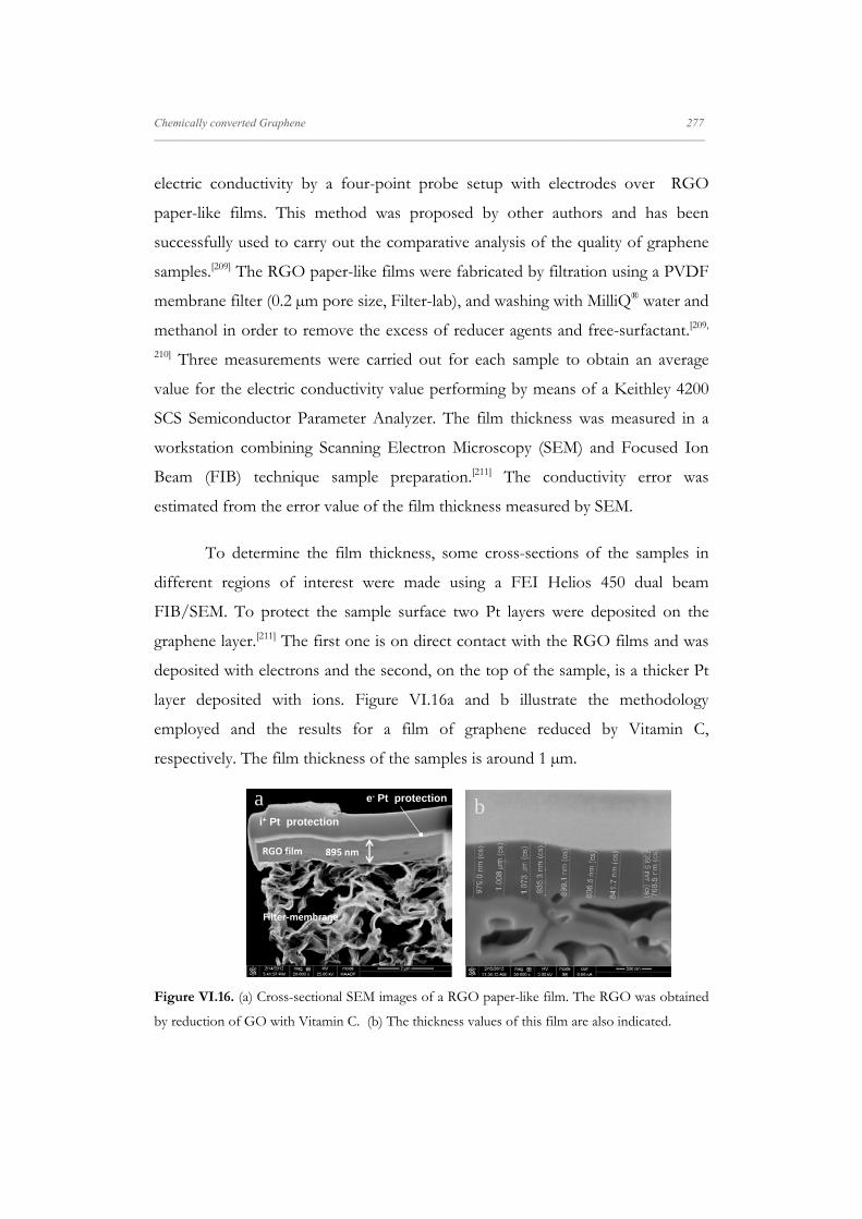
Chemically converted Graphene 277 _____________________________________________________________________________________________________________________
electric conductivity by a four-point probe setup with electrodes over RGO
paper-like films. This method was proposed by other authors and has been
successfully used to carry out the comparative analysis of the quality of graphene
samples.[209] The RGO paper-like films were fabricated by filtration using a PVDF
membrane filter (0.2 µm pore size, Filter-lab), and washing with MilliQ® water and
methanol in order to remove the excess of reducer agents and free-surfactant.[209,
210] Three measurements were carried out for each sample to obtain an average
value for the electric conductivity value performing by means of a Keithley 4200
SCS Semiconductor Parameter Analyzer. The film thickness was measured in a
workstation combining Scanning Electron Microscopy (SEM) and Focused Ion
Beam (FIB) technique sample preparation.[211] The conductivity error was
estimated from the error value of the film thickness measured by SEM.
To determine the film thickness, some cross-sections of the samples in
different regions of interest were made using a FEI Helios 450 dual beam
FIB/SEM. To protect the sample surface two Pt layers were deposited on the
graphene layer.[211] The first one is on direct contact with the RGO films and was
deposited with electrons and the second, on the top of the sample, is a thicker Pt
layer deposited with ions. Figure VI.16a and b illustrate the methodology
employed and the results for a film of graphene reduced by Vitamin C,
respectively. The film thickness of the samples is around 1 µm.
Figure VI.16. (a) Cross-sectional SEM images of a RGO paper-like film. The RGO was obtained
by reduction of GO with Vitamin C. (b) The thickness values of this film are also indicated.
895 nmRGO film
Filter‐membrane
i+ Pt protection
e- Pt protectiona b

278 Chemically converted Graphene _____________________________________________________________________________________________________________________
The electric conductivity values of the different samples are collected in
Table VI.2. The conductivity value of RGO sheets reduced by hydrazine agrees
with values obtained previously by other authors.[165, 403] We cannot compare our
values for sheets reduced by Vitamin C with values in the literature, because the
values found correspond to samples reduced by Vitamin C with a subsequent
thermal annealing step. This annealing step can remove the oxidized form of the
Vitamin C attached to the network increasing the conductivity of sheets.[165] The
conductivity values in Table VI.2 show that the RGO sample reduced by Vitamin
C is less conductive than the one reduced by hydrazine. This is an unexpected
result if one considers that the Csp2 percentages are similar in both samples while
the ID/IG ratio is smaller for the RGO reduced by Vitamin C. This picture can be
explained if one considers that the residual O-containing groups in the case of
samples reduced by Vitamin C, detected by the increase of the O/C ratio, destroy
the graphene structure and promote a loss of conductivity.[403]
From our results it is noteworthy that the functionalization with the
zwitterionic surfactant DDPS increases the conductivity for samples reduced by
both, hydrazine and Vitamin C. This is consistent with the high values of the
percentage of Csp2 of functionalized RGO samples, see Table VI.2, and with the
decrease of the N/C (hydrazine) and O/C (Vitamin C) ratios, Table VI.1 for the
functionalized RGO samples. The surfactant adsorption on the GO sheets can be
responsible for this behaviour. Thus, when the GO flakes are dispersed in the
surfactant aqueous solution by sonication, the adsorbed surfactants molecules
avoid the restacking by steric repulsion, favouring the reduction process.[453]
Additionally, the surfactant adsorbed on the sheets also avoids the restacking of
the RGO sheets obtained during the reduction process.
Finally, the high electric conductivity values of the functionalized sheets
can be explained if one considers that the functionalization by DDPS via

Chemically converted Graphene 279 _____________________________________________________________________________________________________________________
hydrophobic interactions with the graphitic networks provides interconnected
network of RGO with demonstrated high conductivity.[454]
Moreover, the conductivity of our functionalized RGO samples is
generally higher than values found in the literature for paper-like films of RGO
functionalized with ionic surfactants.[385, 433, 455] This behaviour can be interpreted if
one takes into account that the zwitterionic surfactants present higher adsorption
on the hydrophobic surfaces than the ionic ones,[399, 400] providing better
stabilization against the restacking process than that obtained by the ionic
surfactants. Besides, the DDPS surfactant improves the conductivity value of
RGO paper-like films functionalized with the zwitterionic surfactant CHAPS.[455]
Structural differences between these surfactants can be responsible for this
behaviour. Thus, our results suggest stronger interactions between the
hydrophobic moiety of DDPS and RGO than between the hydrophobic part of
CHAPS and the RGO carbon network. This fact can be due to the more
hydrophilic character of the surfactant CHAPS.[402]
VI.2.6. Electron Beam Lithography: RGO sheets Au-contacted
In order to carry out an electrical characterization of the RGO sheets, we
decided to contact the LB deposited sheets with Ti/Au electrodes on silicon
wafers by electron beam lithography (EBL) technique. The electrodes were
designed with a 300-1000 nm separation in Van der Pauw and Hall-bar geometry,
that allows performing electrical measurements at different geometries.
Thus, we selected three sheets as representative sampling of each kind of
RGO samples: reduction with hydrazine functionalized with DDPS, Vitamin C
and Vitamin C functionalized with DDPS (Figure VI.17). We did not select the
RGO reduced in situ with hydrazine, because the silicon oxide layer is damaged
during the reduction process, and it may generate problems with the metal

280 Chemically converted Graphene _____________________________________________________________________________________________________________________
adhesion on the wafer and does not guarantee the complete isolation with the
silicon for the electrical measurements.
To design the electrodes, the main limitation was the size of the flakes. We
used an optical microscope to take the measurements for the "flake" outline over
which we design the electrodes geometry. As the microscope has a resolution of
micrometers, we can only select the flakes greater than 5 µm. All the samples
prepared have several flakes with this size condition.
Figure VI.17. Optic microscope and SEM images of different RGO sheets before and after the
Au/Ti electrodes deposition: reduced with hydrazine in the presence of DDPS (a, b, c); Vitamin C
(d, e, f) and Vitamin C in the presence of DDPS (g, h, i). The arrows are a visual guide to localize
the RGO sheets due to the optical contrast of the images is not sufficient.
a b c
d e f
g h i
10 µm 10 µm
10 µm
10 µm
5 µm
5 µm
Chemically converted Graphene 281 _____________________________________________________________________________________________________________________
The electrical measurements were carried out in a four probe station by
the Van der Pauw method. However, we obtained high resistivity values out of
the equipment range for the different samples not allowing the material
characterization. This fact can be due to a bad contact between the Ti/Au
electrodes and the RGO samples. Although, this contact has been successfully
used for pristine graphene samples obtained by micromechanical exfoliation.[456, 457]
However, our samples present oxygen, nitrogen or sulphur groups functionalizing
the hexagonal network, therefore the contact is not good enough. In a future, it is
necessary to investigate other metal contacts to improve the electrical
measurements.[458]


VII. Conclusions


Conclusions 283 _____________________________________________________________________________________________________________________
VII. Conclusions
In this chapter we summarized the main conclusions achieved from the
experimental results of the following systems studied in this work: monolayers of
anhydride maleic polymer derivatives, films of CdSe QDs and chemically derived
graphene deposited onto solids by the Langmuir-Blodgett methodology.
In the case of the polymers, Chapter IV, the study was focused on the
self-assembly at the air-water interface and onto solids. In order to prepare films
supported with potential applications in the construction of electronic devices, we
were interested in studying the effect of electrolytes on the equilibrium and
dynamic properties of Langmuir and Langmuir-Blodgett films of the polymer poly
(styrene-co-maleic anhydride) partial 2 buthoxy ethyl ester cumene terminated,
PS-MA-BEE. Results show that the Langmuir films deposited on saline solutions
are more expanded and stable than the monolayer without salt in the subphase.
These facts can be attributed to the formation of a complex between the divalent
cation, Mg2+, and the carboxylic groups of the polymer molecule. Our results
demonstrate that the polymer-Mg2+ complexes increase the viscoelastic behaviour
of the monolayer.
Results also demonstrate surface self-assembly processes for dense
polymer monolayers. The aggregates transferred from the air-liquid interface onto
silicon wafers present different morphologies depending on the methodology
employed to build the LB film and the subphase composition. The thickness of
the LB films obtained by ellipsometry agrees with the film height determined by
AFM measurements.
Moreover, in order to reinforce the complex formation between Mg2+ and
polymer acid groups, we studied surface properties of other anhydride maleic
derivative polymer without carboxylic acid groups. The copolymer chosen was
poly (styrene-co-maleic anhydride) cumene terminated, PS-b-MA. Results show
284 Conclusions _____________________________________________________________________________________________________________________
the characteristic effect of electrolytes on the water-insoluble monolayers, i.e. the
isotherms is shifted to smaller areas when the salt concentration in the subphase
increases. This is a signature of no complexation. On the other hand, the
morphology of the LB films depends on the polymer nature, stripes for PS-MA-
BEE and circular domains for PS-b-MA molecules.
In addition, the polymer PS-b-MA allows us to carry out the study of the
2D glass transition temperature (Tg) by means of equilibrium and dynamics
properties. The surface potential measurements indicate that the presence of
electrolytes in the aqueous subphase does not strongly modify the 2D Tg. Finally,
the phase transition in PS-b-MA monolayers was highlighted by dynamic
measurements. Results show that the glass state presents higher elasticity modulus
and viscosity values than the fluid state.
In the study of the QDs films, presented in Chapter V, our aim was to
develop different approaches to prepare QDs films by means of the Langmuir-
Blodgett technique and to study the influence of the film morphology on the film
photoluminescence properties. To assist the QDs self-assembly the polymer PS-
MA-BEE was used. Three different approaches were employed.
In the first one, referred to as co-spreading methodology, we study the
assembly ability of QD/PS-MA-BEE mixed monolayers onto solids by AFM and
TEM images. Results obtained demonstrate that the surface state of the block
copolymer PS-MA-BEE plays a decisive role on the morphology of the QDs
assemblies. Thus, when the Langmuir monolayer precursor of the LB films
presents the smallest elasticity value, corresponding to the polymer brush
conformation at the surface, the films are composed by hexagonal networks with
QDs adsorbed on the rims. Conversely, monolayers with the highest elasticity
values give LB films with QD/polymer domains. The different architectures were
interpreted in terms of distinct dewetting processes, nucleation and growth of
holes for the formation of hexagonal networks and spinodal dewetting, for
Conclusions 285 _____________________________________________________________________________________________________________________
QD/polymer domains. Our results demonstrate that it is possible to modulate the
morphology of the QDs LB films by modifying both, the surface composition
and the elastic properties of the Langmuir monolayer precursors of the LB films.
This strategy could be presented as a non-template reproducible technique for
patterning at the nanoscale.
In the second approach, the polymer LB film is used to modify the surface
properties of the substrate. Results demonstrate that the LB film of the polymer
PS-MA-BEE plays a decisive role in the increase of the surface density of QDs
adsorbed on mica. Cohesive interactions between the polymer chains and the
hydrocarbon moieties of the QDs stabilizer, TOPO, can be the origin of this fact.
In all cases island-like QDs 2D aggregates were observed and the nanoparticle 3D
agglomeration is avoided.
Finally, we proposed to study the influence of the QDs ligand nature on
the nanoparticles assembly by exchanging the QDs’ ligand by the polymer, PS-
MA-BEE. In this way, QD/PS-MA-BEE mixed films and bilayers PS-MA-
BEE//QDs were prepared. Results show that the replacement of the QDs
stabilizer TOPO by the polymer PS-MA-BEE affects the morphology of the
nanoparticles self-assemblies. In the case of mixed films, the high molecular
weight of the film formed by QDP nanoparticles, favours the gravitational effects
against the capillary wave effects. Therefore, the morphology of the self-
assemblies is driven by dewetting mechanism of nucleation and growth of holes.
According to the results, it is possible to modulate the morphology of the QDs
LB films by combining the modification of both the nanoparticle capping ligand
and the surface composition of the Langmuir monolayer precursors of the LB
films. In the case of bilayers, as the QDs’ ligand and the coating film exposed the
same group, PS, favourable interactions lead to a better spreading of the QDs on
polymer film.

286 Conclusions _____________________________________________________________________________________________________________________
Our results suggest that the monolayer compression develops transient
metastable states that finally relax towards the minimum energy configuration of
the domain. Therefore, to achieve the stable state we applied successive
compression-expansion cycles and then the barriers were stopped. Using this
approach more ordered nanoparticles monolayers were obtained. Moreover, this
methodology allows us to obtain information of the different relaxation processes
produced after the compression-expansion cycles. Results show two relaxation
processes for QDs and mixed QD/polymer films. The fastest one was ascribed to
rafts movement, while the slowest one was related to movements inside rafts.
Moreover, the time-scales of these processes are related to the film composition.
Thus, slower relaxations correspond to systems with high polymer mole fraction.
Finally, we suggest shearing as a driving force to direct the assembly of
nanocomposite films according to the stress-direction orientation of the
QD/polymer films observed. Moreover, in this work we have proposed the
combination of two direction-controlling methods: a polymer matrix and a
shearing external force to assemble the nanocomposite.
Our results demonstrate that it is possible to modulate the QDs assembly
by choosing the proper methodology.
Finally, we analyzed the effect of the QDs domains morphology on the
film photoluminescence properties by means of FLIM. The photoluminescence
time-resolved study of the films has allowed us to highlight several QD
photodynamic phenomena in the LB films.
To interpret the results obtained for the different LB films we previously
studied the dynamic photoluminescence emission of QDs dissolved in
chloroform. Results demonstrate that the particles average lifetime in solution is
independent of polymer concentration, thus, a static quenching process by charge-
transfer has been proposed. On the other hand, the PL decay curves for QDs are
different in solution vs. in LB films. As it is expected, the solution offers a more

Conclusions 287 _____________________________________________________________________________________________________________________
fluid environment minimizing the QDs interaction, while the LB films present a
different dielectric environment that increases the radiative lifetime and a compact
particle arrangement that allows for QD-QD dipole interaction. On the other
hand, studies carried out by analyzing the effect of the excitation energy, the time
exposure and the spectral emission region collected on the PL dynamics
highlighted the existence of multi-excitonic processes, a quasi-reversible photo-
passivation of the particle surface and the surface-defects emission, respectively.
The photoluminescence of QD/polymer mixed films was characterized
for different conditions of film deposition: bilayer or co-spreading; QD-to-
polymer composition; and surface pressure at deposition. Results show that the
photoluminescence dynamics of QD films are affected by energy transport and
trapping processes occurring in the compact arrangement of QDs deposited. The
efficiency of these processes essentially depends on inter-dot distance and on
surface density of energy traps, which can be QDs with extensive surface defects
or small aggregated clusters. Among the several conditions studied, the bilayer
deposition yielded the surfaces with more emission intensity, i.e. more brightness.
The simultaneous analysis of PL decays and TEM images allowed us to relate this
behaviour to a lower amount of QD clustering in the bilayer film. The model used
for decay analysis considers energy transport and trapping in the films and,
although it is only an approximate model, it also allowed us to relate the
photoluminescence dynamics to film morphology. Indeed, the concentration of
traps retrieved from decay analysis for the bilayer film is about half of those in co-
spreading films. Finally, from our results it is possible to conclude that in order to
improve the photoluminescence properties of QD films, it is paramount to obtain
films with regular and compact morphology and to minimize QD clustering.
The last system studied was chemically derived graphene, Chapter VI.
The aims were to develop a new synthetic route by using the zwitterionic
surfactant dodecyl dimethyl ammonium propane sulphonate, DDPS, and to

288 Conclusions _____________________________________________________________________________________________________________________
deposit the material prepared in a controlled way in order to achieve good quality
and few-layer RGO sheets. Therefore, we simultaneously analyzed the reduction
degree, the defect repair degree and the electric conductivity of the RGO sheets
obtained by reduction of GO by hydrazine and Vitamin C and functionalized by
the surfactant DDPS. Our results demonstrate that the functionalization with the
zwitterionic surfactant DDPS improves the reduction efficiency of hydrazine and
Vitamin C measured by the percentage of Csp2; reduces the residual groups
attached to the carbon network introduced by the reducer agents in both cases;
and increases the conductivity of the RGO. Moreover, the electrical conductivity
observed in our functionalized samples is generally higher than other surfactant-
functionalized RGO paper-like films. Accordingly, we propose the DDPS
functionalization of RGO as a good non-covalent functionalization, which
increases the electrical conductivity without altering the carbon network.
Furthermore, the functionalization with a zwitterionic surfactant offers a residual
charge that can bind the RGO sheets with other materials in order to prepare
nanocomposites with multiple applications. In addition, results also show that
the Langmuir-Blodgett technique allowed us to deposit a few-layer thick RGO
flakes onto silicon wafers.

VIII. References


References 289 _____________________________________________________________________________________________________________________
VIII. References
1. Petty, M. C., Langmuir-Blodgett Films: An Introduction. Cambridge University
Press: 1996.
2. Bardosova, M.; Pemble, M. E.; Povey, I. M.; Tredgold, R. H., The
Langmuir-Blodgett Approach to Making Colloidal Photonic Crystals from Silica
Spheres. Adv. Mater. 2010, 22 (29), 3104-3124.
3. Park, J. Y.; Advincula, R. C., Nanostructuring Polymers, Colloids, and
Nanomaterials at the Air-Water Interface through Langmuir and Langmuir-
Blodgett Techniques. Soft Matter 2011, 7 (21), 9829-9843.
4. Reiter, G., Probing Properties of Polymers in Thin Films. Adv. Polym. Sci.
2013, 252, 29-64.
5. Jones, R.; Winter, C. S.; Tredgold, R. H.; Hodge, P.; Hoorfar, A., Electron-
beam Resists from Langmuir-Blodgett films of Poly(styrene/maleic anhydride)
Derivatives. Polymer 1987, 28 (10), 1619-1626.
6. Collins, S. J.; Mary, N. L.; Radhakrishnan, G.; Dhathathreyan, A., Studies
of Spread Monolayers of Derivative of Styrene-Maleic Anhydride Copolymers. J.
Chem. Soc. Faraday Trans. 1997, 93 (22), 4021-4023.
7. Rogach, A. L., Semiconductor Nanocrystal Quantum Dots: Synthesis, Assembly,
Spectroscopy and Applications. Springer:Wien: New York, 2008.
8. Tomczak, N.; Jaczewski, D.; Han, M.; Vancso, G. J., Designer Polymer-
Quantum Dot Architectures. Prog. Polym. Sci. 2009, 34 (5), 393-430.
9. Talapin, D. V.; Lee, J.-S.; Kovalenko, M. V.; Shevchenko, E. V., Prospects
of Colloidal Nanocrystals for Electronic and Optoelectronic Applications. Chem.
Rev. 2010, 110 (1), 389-458.
10. Kim, T.-H.; Cho, K.-S.; Lee, E. K.; Lee, S. J.; Chae, J.; Kim, J. W.; Kim, D.
H.; Kwon, J.-Y.; Amaratunga, G.; Lee, S. Y.; Choi, B. L.; Kuk, Y.; Kim, J. M.;
Kim, K., Full-colour Quantum Dot Displays fabricated by Transfer Printing. Nat.
Photon. 2011, 5 (3), 176-182.

290 References _____________________________________________________________________________________________________________________
11. Selinsky, R. S.; Ding, Q.; Faber, M. S.; Wright, J. C.; Jin, S., Quantum Dot
Nanoscale Heterostructures for Solar Energy Conversion. Chem. Soc. Rev. 2013, 42
(7), 2963-2985.
12. Balazs, A. C., Interactions of Nanoscopic Particles with Phase-separating
Polymeric Mixtures. Curr. Opin. Colloid Interface Sci. 1999, 4 (6), 443-448.
13. Lin, Y.; Böker, A.; He, J.; Sill, K.; Xiang, H.; Abetz, C.; Li, X.; Wang, J.;
Emrick, T.; Long, S.; Wang, Q.; Balazs, A.; Russell, T. P., Self-directed Self-
assembly of Nanoparticle/Copolymer Mixtures. Nature 2005, 434 (7029), 55-59.
14. Cheyne, R. B.; Moffitt, M. G., Hierarchical Nanoparticle/Block
Copolymer Surface Features via Synergistic Self-Assembly at the Air-Water
Interface. Langmuir 2005, 21 (23), 10297-10300.
15. Li, H.; Sachsenhofer, R.; Binder, W. H.; Henze, T.; Thurn-Albrecht, T.;
Busse, K.; Kressler, J., Hierarchical Organization of Poly(ethylene oxide)-block-
poly(isobutylene) and Hydrophobically Modified Fe2O3 Nanoparticles at the
Air/Water Interface and on Solid Supports. Langmuir 2009, 25 (14), 8320-8329.
16. Murray, C. B.; Kagan, C. R.; Bawendi, M. G., Synthesis and
Characterization of Monodisperse Nanocrystals and Close-packed Nanocrystal
Assemblies. Annu. Rev. Mater. Sci. 2000, 30 (1), 545-610.
17. Worfolk, B. J.; Rider, D. A.; Elias, A. L.; Thomas, M.; Harris, K. D.;
Buriak, J. M., Bulk Heterojunction Organic Photovoltaics Based on Carboxylated
Polythiophenes and PCBM on Glass and Plastic Substrates. Adv. Funct. Mater.
2011, 21 (10), 1816-1826.
18. Kim, J. Y.; Raja, S.; Stellacci, F., Evolution of Langmuir Film of
Nanoparticles Through Successive Compression Cycles. Small 2011, 7 (17), 2526-
2532.
19. Cicuta, P.; Vella, D., Granular Character of Particle Rafts. Phys. Rev. Lett.
2009, 102 (13), 138302.
20. Zang, D.; Langevin, D.; Binks, B. P.; Wei, B., Shearing Particle
Monolayers: Strain-rate Frequency Superposition. Phys. Rev. E 2010, 81 (1),
011604.

References 291 _____________________________________________________________________________________________________________________
21. Guzmán, E.; Liggieri, L.; Santini, E.; Ferrari, M.; Ravera, F., Effect of
Hydrophilic and Hydrophobic Nanoparticles on the Surface Pressure Response of
DPPC Monolayers. J. Phys. Chem. C 2011, 115 (44), 21715-21722.
22. Ndoro, T. V. M.; Böhm, M. C.; Müller-Plathe, F., Interface and Interphase
Dynamics of Polystyrene Chains near Grafted and Ungrafted Silica Nanoparticles.
Macromolecules 2012, 45 (1), 171-179.
23. Toepperwein, G. N.; Riggleman, R. A.; de Pablo, J. J., Dynamics and
Deformation Response of Rod-Containing Nanocomposites. Macromolecules 2012,
45 (1), 543-554.
24. Osman, A. F.; Edwards, G. A.; Schiller, T. L.; Andriani, Y.; Jack, K. S.;
Morrow, I. C.; Halley, P. J.; Martin, D. J., Structure-Property Relationships in
Biomedical Thermoplastic Polyurethane Nanocomposites. Macromolecules 2012, 45
(1), 198-210.
25. Jones, M.; Scholes, G. D., On the Use of Time-Resolved
Photoluminescence as a Probe of Nanocrystal Photoexcitation Dynamics. J.
Mater. Chem. 2010, 20 (18), 3533-3538.
26. Chen, D.; Feng, H.; Li, J., Graphene Oxide: Preparation,
Functionalization, and Electrochemical Applications. Chem. Rev. 2012, 112 (11),
6027-6053.
27. Hu, W.; Peng, C.; Luo, W.; Lv, M.; Li, X.; Li, D.; Huang, Q.; Fan, C.,
Graphene-Based Antibacterial Paper. ACS Nano 2010, 4 (7), 4317-4323.
28. Cui, X.; Zhang, C.; Hao, R.; Hou, Y., Liquid-phase Exfoliation,
Functionalization and Applications of Graphene. Nanoscale 2011, 3 (5), 2118-2126.
29. Singh, V.; Joung, D.; Zhai, L.; Das, S.; Khondaker, S. I.; Seal, S., Graphene
based Materials: Past, Present and Future. Prog. Mater. Sci. 2011, 56 (8), 1178-1271.
30. Shao, Y.; Wang, J.; Wu, H.; Liu, J.; Aksay, I. A.; Lin, Y., Graphene Based
Electrochemical Sensors and Biosensors: A Review. Electroanalysis 2010, 22 (10),
1027-1036.
292 References _____________________________________________________________________________________________________________________
31. Rao, C. N. R.; Cheetham, A. K., Materials Science at the Nanoscale. In
Nanomaterials Handbook, Gogotsi, Y., Ed. Taylor & Francis Group: New York,
2006.
32. Dutta, J.; Hofmann, H., Self-organization of Colloidal Nanoparticles. In
Encyclopedia of Nanoscience and Nanotechnology, Nalwa, H. S., Ed. American Scientific
Publishers: New York, 2011; Vol. X, pp 1-23.
33. Bloch, J. M.; Yun, W., Condensation of Monovalent and Divalent Metal
Ions on a Langmuir Monolayer. Phys. Rev. A 1990, 41 (2), 844-862.
34. Knipping, E. M.; Lakin, M. J.; Foster, K. L.; Jungwirth, P.; Tobias, D. J.;
Gerber, R. B.; Dabdub, D.; Finlayson-Pitts, B. J., Experiments and Simulations of
Ion-Enhanced Interfacial Chemistry on Aqueous NaCl Aerosols. Science 2000, 288
(5464), 301-306.
35. Laskin, A.; Gaspar, D. J.; Wang, W.; Hunt, S. W.; Cowin, J. P.; Colson, S.
D.; Finlayson-Pitts, B. J., Reactions at Interfaces As a Source of Sulfate Formation
in Sea-Salt Particles. Science 2003, 301 (5631), 340-344.
36. Hamley, I. W., Nanotechnology with Soft Materials. Angew. Chem. Int. Ed.
2003, 42 (15), 1692-1712.
37. Grzelczak, M.; Vermant, J.; Furst, E. M.; Liz-Marzán, L. M., Directed Self-
Assembly of Nanoparticles. ACS Nano 2010, 4 (7), 3591-3605.
38. Whitesides, G. M., Self-assemblying Materials. Sci. Am. 1995, 273, 146-
149.
39. Whitesides, G. M.; Boncheva, M., Beyond Molecules: Self-assembly of
Mesoscopic and Macroscopic Components. Proc. Natl. Acad. Sci. USA 2002, 99
(8), 4769-4774.
40. Yin, J. S.; Wang, Z. L., Handbook of Nanophase and Nanostructured Materials.
Kluwer Academic/Plenum Publishers, Tsinghua University Press,: New York,
2003; Vol. 4.
41. Cheyne, R. B.; Moffitt, M. G., Novel Two-Dimensional “Ring and Chain”
Morphologies in Langmuir−Blodgett Monolayers of PS-b-PEO Block

References 293 _____________________________________________________________________________________________________________________
Copolymers: Effect of Spreading Solution Concentration on Self-Assembly at the
Air−Water Interface. Langmuir 2005, 21 (12), 5453-5460.
42. Rabani, E.; Reichman, D. R.; Geissler, P. L.; Brus, L. E., Drying-mediated
Self-assembly of Nanoparticles. Nature 2003, 426 (6964), 271-274.
43. Martin, C. P.; Blunt, M. O.; Moriarty, P., Nanoparticle Networks on
Silicon: Self-Organized or Disorganized? Nano Lett. 2004, 4 (12), 2389-2392.
44. Gentili, D.; Foschi, G.; Valle, F.; Cavallini, M.; Biscarini, F., Applications
of Dewetting in Micro and Nanotechnology. Chem. Soc. Rev. 2012, 41 (12), 4430-
4443.
45. Xue, L.; Han, Y., Inhibition of Dewetting of Thin Polymer Films. Prog.
Materials Sci. 2012, 57 (6), 947-979.
46. Böker, A.; He, J.; Emrick, T.; Russell, T. P., Self-assembly of
Nanoparticles at Interfaces. Soft Matter 2007, 3 (10), 1231-1248.
47. Stine, K. J.; Moore, B. G., Langmuir Monolayers: Fundamentals and
Relevance to Nanotechnology. In Nano-Surface Chemistry, Rosoff, M., Ed. Marcel
Dekker: New York, 2002.
48. Xiao, L.; Zhou, R.; He, Y.; Li, Y.; Yeung, E. S., Direct Observation of
Nanoparticle Self-Assembly Dynamics at the Water−Air Interface Using
Differential Interference Contrast Microscopy. J. Phys. Chem. C 2009, 113 (4),
1209-1216.
49. Clemente-León, M.; Ito, T.; Yashiro, H.; Yamase, T.; Coronado, E.,
Langmuir−Blodgett Films of a Mo-Blue Nanoring
[Mo142O429H10(H2O)49(CH3CO2)5(CH3CH2CO2)]30 - (Mo142) by the Semiamphiphilic
Method. Langmuir 2007, 23 (7), 4042-4047.
50. Rybak, B. M.; Ornatska, M.; Bergman, K. N.; Genson, K. L.; Tsukruk, V.
V., Formation of Silver Nanoparticles at the Air−Water Interface Mediated by a
Monolayer of Functionalized Hyperbranched Molecules. Langmuir 2006, 22 (3),
1027-1037.

294 References _____________________________________________________________________________________________________________________
51. Kinge, S.; Crego-Calama, M.; Reinhoudt, D. N., Self-Assembling
Nanoparticles at Surfaces and Interfaces. ChemPhysChem 2008, 9 (1), 20-42.
52. Yang, P.; Kim, F., Langmuir–Blodgett Assembly of One-Dimensional
Nanostructures. ChemPhysChem 2002, 3 (6), 503-506.
53. Kim, H.-C.; Park, S.-M.; Hinsberg, W. D., Block Copolymer Based
Nanostructures: Materials, Processes, and Applications to Electronics. Chem. Rev.
2010, 110 (1), 146-177.
54. Gonçalves da Silva, A. M.; Filipe, E. J. M.; d'Oliveira, J. M. R.; Martinho, J.
M. G., Interfacial Behavior of Poly(styrene)−Poly(ethylene oxide) Diblock
Copolymer Monolayers at the Air−Water Interface. Hydrophilic Block Chain
Length and Temperature Influence. Langmuir 1996, 12 (26), 6547-6553.
55. Cox, J. K.; Yu, K.; Constantine, B.; Eisenberg, A.; Lennox, R. B.,
Polystyrene−Poly(ethylene oxide) Diblock Copolymers Form Well-Defined
Surface Aggregates at the Air/Water Interface. Langmuir 1999, 15 (22), 7714-7718.
56. Devereaux, C. A.; Baker, S. M., Surface Features in Langmuir−Blodgett
Monolayers of Predominantly Hydrophobic Poly(styrene)−Poly(ethylene oxide)
Diblock Copolymer. Macromolecules 2002, 35 (5), 1921-1927.
57. Cheyne, R. B.; Moffitt, M. G., Self-Assembly of Polystyrene-block-
Poly(Ethylene Oxide) Copolymers at the Air−Water Interface: Is Dewetting the
Genesis of Surface Aggregate Formation? Langmuir 2006, 22 (20), 8387-8396.
58. Discher, D. E.; Eisenberg, A., Polymer Vesicles. Science 2002, 297 (5583),
967-973.
59. Zhao, L.; Byun, M.; Rzayev, J.; Lin, Z., Polystyrene−Polylactide
Bottlebrush Block Copolymer at the Air/Water Interface. Macromolecules 2009, 42
(22), 9027-9033.
60. Seo, Y.; Paeng, K.; Park, S., Molecular Weight Effect on the Behaviors of
Polystyrene-block-poly(methyl methacrylate) Diblock Copolymers at Air/Water
Interface. Macromolecules 2001, 34 (25), 8735-8744.

References 295 _____________________________________________________________________________________________________________________
61. Chung, B.; Choi, M.; Ree, M.; Jung, J. C.; Zin, W. C.; Chang, T., Subphase
pH Effect on Surface Micelle of Polystyrene-b-poly(2-vinylpyridine) Diblock
Copolymers at the Air−Water Interface. Macromolecules 2006, 39 (2), 684-689.
62. Liu, G.; Yang, S.; Zhang, G., Conformational Changes of Poly(N-
isopropylacrylamide) Chains at Air/Water Interface: Effects of Temperature,
Compression Rate, and Packing Density. J. Phys. Chem. B 2007, 111 (14), 3633-
3639.
63. Zhao, L.; Lin, Z., Self-assembly of Non-linear Polymers at the Air/Water
Interface: The Effect of Molecular Architecture. Soft Matter 2011, 7 (22), 10520-
10535.
64. Rosi, N. L.; Mirkin, C. A., Nanostructures in Biodiagnostics. Chem. Rev.
2005, 105 (4), 1547-1562.
65. Tang, Z.; Kotov, N. A., One-Dimensional Assemblies of Nanoparticles:
Preparation, Properties, and Promise. Adv. Mater. 2005, 17 (8), 951-962.
66. Zhang, L.; Gaponik, N.; Müller, J.; Plate, U.; Weller, H.; Erker, G.; Fuchs,
H.; Rogach, A. L.; Chi, L., Branched Wires of CdTe Nanocrystals Using
Amphiphilic Molecules as Templates. Small 2005, 1 (5), 524-527.
67. Gattás-Asfura, K. M.; Constantine, C. A.; Lynn, M. J.; Thimann, D. A.; Ji,
X.; Leblanc, R. M., Characterization and 2D Self-Assembly of CdSe Quantum
Dots at the Air−Water Interface. J. Am. Chem. Soc. 2005, 127 (42), 14640-14646.
68. Ji, X.; Wang, C.; Xu, J.; Zheng, J.; Gattás-Asfura, K. M.; Leblanc, R. M.,
Surface Chemistry Studies of (CdSe)ZnS Quantum Dots at the Air−Water
Interface. Langmuir 2005, 21 (12), 5377-5382.
69. Lambert, K.; C apek, R. K.; Bodnarchuk, M. I.; Kovalenko, M. V.; Van
Thourhout, D.; Heiss, W.; Hens, Z., Langmuir−Schaefer Deposition of Quantum
Dot Multilayers. Langmuir 2010, 26 (11), 7732-7736.
70. Gole, A.; Jana, N. R.; Selvan, S. T.; Ying, J. Y., Langmuir−Blodgett Thin
Films of Quantum Dots: Synthesis, Surface Modification, and Fluorescence
Resonance Energy Transfer (FRET) Studies. Langmuir 2008, 24 (15), 8181-8186.

296 References _____________________________________________________________________________________________________________________
71. Deshmukh, R. D.; Buxton, G. A.; Clarke, N.; Composto, R. J., Nanoscale
Block Copolymer Templates Decorated by Nanoparticle Arrays. Macromolecules
2007, 40 (17), 6316-6324.
72. Hernández, M.-P.; Monroy, F.; Ortega, F.; Rubio, R. G.; Martín-
Domenech, Á.; Priego, E. M.; Sánchez, L.; Martín, N., An Experimental Study of
the Stability and Dynamics of Langmuir Films of Fullerene Derivatives and Their
Mixtures with Pentadecanoic Acid. Langmuir 2001, 17 (11), 3317-3328.
73. Nierengarten, J.-F., Chemical Modification of C60 for Materials Science
Applications. New J. Chem. 2004, 28 (10), 1177-1191.
74. Kim, Y.; Minami, N.; Zhu, W.; Kazaoui, S.; Azumi, R.; Matsumoto, M.,
Langmuir-Blodgett Films of Single-wall carbon Nanotubes: Layer-by-Layer
Deposition and in-plane Orientation of Tubes. Jpn. J. Appl. Phys. 2003, 42, 7629-
7634.
75. Li, X.; Zhang, G.; Bai, X.; Sun, X.; Wang, X.; Wang, E.; Dai, H., Highly
Conducting Graphene Sheets and Langmuir-Blodgett Films. Nat. Nanotechnol.
2008, 3 (9), 538-542.
76. Cote, L. J.; Kim, F.; Huang, J., Langmuir-Blodgett Assembly of Graphite
Oxide Single Layers. J. Am. Chem. Soc. 2009, 131 (3), 1043-1049.
77. Tabor, D., Babylonian Lecanomancy: An Ancient Text on the Spreading
of Oil on Water. J. Colloid Interface Sci. 1980, 75 (1), 240-245.
78. Chambers, A., The Japanese Art of Marbling. Thames & Hudson: 1993.
79. Dynarowicz-Latka, P.; Dhanabalan, A.; Oliveira Jr, O. N., Modern
Physicochemical Research on Langmuir Monolayers. Adv. Colloid Interface Sci. 2001,
91 (2), 221-293.
80. Franklin, B.; Brownrigg, W.; Farish, M., Of the Stilling of Waves by means
of Oil. Extracted from Sundry Letters between Benjamin Franklin, LL. D. F. R. S.
William Brownrigg, M. D. F. R. S. and the Reverend Mr. Farish. Phil. Trans. Res.
Soc. (London) 1774, 64, 445-460.
81. Rayleigh, L., On the Superficial Viscosity of Water. Proc. R. Soc. Ser. A
1890, 48, 127-140.

References 297 _____________________________________________________________________________________________________________________
82. Pockels, A., Surface Tension. Nature 1891, 43, 437-439.
83. Rayleigh, L., XXXVI. Investigations in Capillarity:—The Size of Drops.—
The Liberation of Gas from Supersaturated Solutions.—Colliding Jets.—The
Tension of Contaminated Water-Surfaces. Phil. Mag. Series 5 1899, 48 (293), 321-
337.
84. Langmuir, I., The Constitution and Fundamental Properties of Solids and
Liquids. II. Liquids. J. Am. Chem. Soc. 1917, 39 (9), 1848-1906.
85. Langmuir, I., The Mechanism of the Surface Phenomena of Flotation.
Trans. Faraday Soc. 1920, 15 (June), 62-74.
86. Blodgett, K. B., Films Built by Depositing Successive Monomolecular
Layers on a Solid Surface. J. Am. Chem. Soc. 1935, 57 (6), 1007-1022.
87. Gaines, G. L., Insoluble Monolayers at the Air-Water Interface. Interscience
Publishers: 1966.
88. Jones, R. A. L.; Richards, R. W., Polymers at Surfaces and Interfaces.
Cambridge University Press: United Kingdom, 1999.
89. Stenhagen, E., Determination of Organic Structures by Physical Methods.
Academic Press: New York, 1955.
90. Nutting, G. C.; Harkins, W. D., Pressure-Area Relations of Fatty Acid and
Alcohol Monolayers. J. Am. Chem. Soc. 1939, 61 (5), 1180-1187.
91. Marsden, J.; Rideal, E. K., On Monolayers of Isomeric Unsaturated
Compounds. J. Chem. Soc. 1938, 1163-1171.
92. Dynarowicz-Łatka, P.; Dhanabalan, A.; Oliveira, O. N., A Study on Two-
Dimensional Phase Transitions in Langmuir Monolayers of a Carboxylic Acid
with a Symmetrical Triphenylbenzene Ring System. J. Phys. Chem. B 1999, 103 (29),
5992-6000.
93. Laxhuber, L. A.; Moehwald, H., Thermodesorption Spectroscopy of
Langmuir-Blodgett Films. Langmuir 1987, 3 (5), 837-845.

298 References _____________________________________________________________________________________________________________________
94. Schwartz, D. K.; Viswanathan, R.; Zasadzinski, J. A. N., Commensurate
Defect Superstructures in a Langmuir-Blodgett Film. Phys. Rev. Lett. 1993, 70 (9),
1267-1270.
95. Marčelja, S., Chain Ordering in Liquid Crystals: II. Structure of Bilayer
Membranes. Biochim. Biophys. Acta 1974, 367 (2), 165-176.
96. De Keyser, P.; Joos, P., Desorption at Constant Surface Pressure from
Slightly Soluble Monolayers. J. Colloid Interface Sci. 1983, 91 (1), 131-137.
97. Barros, A. M.; Dhanabalan, A.; Constantino, C. J. L.; Balogh, D. T.;
Oliveira Jr, O. N., Langmuir Monolayers of Lignins obtained with different
Isolation Methods. Thin Solid Films 1999, 354 (1–2), 215-221.
98. Wan Kim, T.; Park, J.-S.; Choi, J.-S.; Kang, D.-Y., π-A Isotherms and
Electrical Properties of Polyamic Acid Alkylamine salts (PAAS) Langmuir-
Blodgett Films. Thin Solid Films 1996, 284–285, 500-504.
99. Hąc-Wydro, K.; Wydro, P.; Dynarowicz-Łątka, P., A Study of the
Interaction between Dialkyldimethylammonium bromides and Tri-n-
octylphosphine oxide (topo) in Mixed Monolayers at the Air/Water Interface. J.
Colloid Interface Sci. 2004, 278 (1), 206-214.
100. Whitten, D. G., Photochemical Reactions in Organized Monolayer
Assemblies. I. Cis-trans Isomerization of Thioindigo Dyes. J. Am. Chem. Soc. 1974,
96 (2), 594-596.
101. Polymeropoulos, E. E.; Möbius, D.; Kuhn, H., Photoconduction in
Monolayer Assemblies with Functional Units of Sensitizing and Conducting
Molecular Components. J. Chem. Phys. 1978, 68 (8), 3918-3931.
102. Shembekar, V. R.; Dhanabalan, A.; Talwar, S. S.; Contractor, A. Q., Study
of Mixed System in Monolayers and Multilayers transferred by Langmuir–
Blodgett Technique. Thin Solid Films 1999, 342 (1–2), 270-276.
103. Kuhn, H., Present Status and Future Prospects of Langmuir-Blodgett Film
Research. Thin Solid Films 1989, 178 (1–2), 1-16.

References 299 _____________________________________________________________________________________________________________________
104. Era, M.; Tsutsui, T.; Saito, S., Control of Chromophore Orientation in
Langmuir-Blodgett Films: Molecular Mixing of two Homologous Amphiphiles.
Langmuir 1989, 5 (6), 1410-1411.
105. Puggelli, M.; Gabrielli, G., Behavior of Vinyl Polymers in Mixed
Monolayers. J. Colloid Interface Sci. 1977, 61 (3), 420-427.
106. Chifu, E.; Zsakó, J.; Tomoaia-Cotişel, M., Xanthophyll Films: I. Single-
component Monolayers at the Air/Water Interface. J. Colloid Interface Sci. 1983, 95
(2), 346-354.
107. Chattoraj, D. K.; Birdi, K. S., Adsorption and the Gibbs Surface Excess,
Plenum Press: New York, 1984; pp 219-223.
108. Costin, I. S.; Barnes, G. T., Two-component Monolayers. II. Surface
Pressure-Area relations for the Octadecanol-docosyl Sulphate System. J. Colloid
Interface Sci. 1975, 51 (1), 106-121.
109. Gálvez Ruiz, M. J.; Cabrerizo Vilchez, M. A., A Study of the Miscibility of
Bile Components in Mixed Monolayers at the Air-Liquid Interface I. Cholesterol,
Lecithin, and Lithocholic Acid. Colloid Polym. Sci. 1991, 269 (1), 77-84.
110. Kuhn, H.; Möbius, D., Monolayer Assemblies. In Investigations of Surfaces
and Interfaces, Rossiter, B. W.; Baetzold, R. C., Eds. John Wiley & Sons: New York,
1993; Vol. IX.
111. Roberts, G., Langmuir-Blodgett Films. Plenum Press New York: 1990.
112. Langmuir, I.; Schaefer, V. J., Activities of Urease and Pepsin Monolayers.
J. Am. Chem. Soc. 1938, 60 (6), 1351-1360.
113. Kossi, C. N.; Leblanc, R. M., Rhodopsin in a New Model Bilayer
Membrane. J. Colloid Interface Sci. 1981, 80 (2), 426-436.
114. Bondarenko, M. P.; Kovalchuk, V. I.; Zholkovskiy, E. K.; Vollhardt, D.,
Concentration Polarization at Langmuir Monolayer Deposition: The Role of
Indifferent Electrolytes. J. Phys. Chem. B 2007, 111 (7), 1684-1692.
300 References _____________________________________________________________________________________________________________________
115. Kovalchuk, V. I.; Bondarenko, M. P.; Zholkovskiy, E. K.; Vollhardt, D.,
Influence of Ion Transfer Kinetics on the Composition of Langmuir−Blodgett
Films. J. Phys. Chem. B 2008, 112 (36), 11333-11340.
116. Honig, E. P., Molecular Constitution of X- and Y-type Langmuir-Blodgett
Films. J. Colloid Interface Sci. 1973, 43 (1), 66-72.
117. Ulman, A., An Introduction to Ultrathin Organic Films From Langmuir-Blodgett to
Self-Assembly. Academic Press, Inc.: San Diego, 1991.
118. Jones, M. N.; Chapman, D., Micelles, Monolayers and Biological Membranes.
John Willey & Sons: New York, 1995.
119. De Gennes, P. G., Scaling Concepts in Polymer Physics. Cornell University
Press, Ithaca: New York, 1979.
120. Flory, P. J., The Configuration of Real Polymer Chains. J. Chem. Phys.
1949, 17 (3), 303-310.
121. Thirumalai, D., Two Landmarks in Polymer Physics: the Edwards Model
and de Gennes' Observation. Theor. Chem. Acc. 2000, 103 (3-4), 292-293.
122. Buzza, D. M. A., General Theory for Capillary Waves and Surface Light
Scattering. Langmuir 2002, 18 (22), 8418-8435.
123. Davies, J. T.; Rideal, E. K., Interfacial Phenomena. Academic Press: New
York, 1963.
124. Gonçalves da Silva, A. M.; Romão, R. S.; Lucero Caro, A.; Rodríguez
Patino, J. M., Memory Effects on the Interfacial Characteristics of
Dioctadecyldimethylammonium bromide Monolayers at the Air–Water Interface.
J. Colloid Interface Sci. 2004, 270 (2), 417-425.
125. Cicuta, P.; Hopkinson, I., Scaling of Dynamics in 2d Semi-dilute Polymer
Solutions. Europhys. Lett. 2004, 68 (1), 65-71.
126. Sukhishvili, S. A.; Chen, Y.; Müller, J. D.; Gratton, E.; Schweizer, K. S.;
Granick, S., Surface Diffusion of Poly(ethylene glycol). Macromolecules 2002, 35 (5),
1776-1784.
127. Wang, X.; Foltz, V. J., Chain Conformation in Two-Dimensional Dense
State. J. Chem. Phys. 2004, 121 (16), 8158-8162.
References 301 _____________________________________________________________________________________________________________________
128. Miranda, B.; Hilles, H. M.; Rubio, R. n. G.; Ritacco, H.; Radic, D.;
Gargallo, L.; Sferrazza, M.; Ortega, F., Equilibrium and Surface Rheology of
Monolayers of Insoluble Polycations with Side Chains. Langmuir 2009, 25 (21),
12561-12568.
129. Vilanove, R.; Rondelez, F., Scaling Description of Two-Dimensional
Chain Conformations in Polymer Monolayers. Phys. Rev. Lett. 1980, 45 (18), 1502-
1505.
130. Hilles, H.; Monroy, F.; Bonales, L. J.; Ortega, F.; Rubio, R. G., Fourier-
Transform Rheology of Polymer Langmuir Monolayers: Analysis of the Non-
linear and Plastic Behaviors. Adv. Colloid Interface Sci. 2006, 122 (1-3), 67-77.
131. Langevin, D.; Monroy, F., Interfacial Rheology of Polyelectrolytes and
Polymer Monolayers at the Air–Water Interface. Curr. Opin. Colloid Interface Sci.
2010, 15 (4), 283-293.
132. Doi, M.; Edwards, S. F., The Theory of Polymer Dynamics. Oxford University
Press: Oxford, 1986.
133. Monroy, F.; Hilles, H. M.; Ortega, F.; Rubio, R. G., Relaxation Dynamics
of Langmuir Polymer Films: A Power-Law Analysis. Phys. Rev. Lett. 2003, 91 (26),
268302.
134. Tolnai, G.; Csempesz, F.; Kabai-Faix, M.; Kálmán, E.; Keresztes, Z.;
Kovács, A. L.; Ramsden, J. J.; Hórvölgyi, Z., Preparation and Characterization of
Surface-Modified Silica-Nanoparticles. Langmuir 2001, 17 (9), 2683-2687.
135. Horozov, T. S.; Aveyard, R.; Clint, J. H.; Binks, B. P., Order−Disorder
Transition in Monolayers of Modified Monodisperse Silica Particles at the
Octane−Water Interface. Langmuir 2003, 19 (7), 2822-2829.
136. Reculusa, S.; Massé, P.; Ravaine, S., Three-dimensional Colloidal Crystals
with a Well-defined Architecture. J. Colloid Interface Sci. 2004, 279 (2), 471-478.
137. van Duffel, B.; Ras, R. H. A.; De Schryver, F. C.; Schoonheydt, R. A.,
Langmuir-Blodgett Deposition and Optical Diffraction of Two-Dimensional
Opal. J. Mater. Chem. 2001, 11 (12), 3333-3336.
302 References _____________________________________________________________________________________________________________________
138. Szekeres, M.; Kamalin, O.; Schoonheydt, R. A.; Wostyn, K.; Clays, K.;
Persoons, A.; Dekany, I., Ordering and Optical Properties of Monolayers and
Multilayers of Silica Spheres deposited by the Langmuir-Blodgett Method. J.
Mater. Chem. 2002, 12 (11), 3268-3274.
139. Xu, J.; Ji, X.; Gattás-Asfura, K. M.; Wang, C.; Leblanc, R. M., Langmuir
and Langmuir–Blodgett Films of Quantum Dots. Colloids Surf. A 2006, 284–285,
35-42.
140. Dabbousi, B. O.; Murray, C. B.; Rubner, M. F.; Bawendi, M. G.,
Langmuir-Blodgett Manipulation of Size-Selected CdSe Nanocrystallites. Chem.
Mater. 1994, 6 (2), 216-219.
141. Kotov, N. A.; Meldrum, F. C.; Wu, C.; Fendler, J. H., Monoparticulate
Layer and Langmuir-Blodgett-Type Multiparticulate Layers of Size-Quantized
Cadmium Sulfide Clusters: A Colloid-Chemical Approach to Superlattice
Construction. J. Phys. Chem. 1994, 98 (11), 2735-2738.
142. Santhanam, V.; Liu, J.; Agarwal, R.; Andres, R. P., Self-Assembly of
Uniform Monolayer Arrays of Nanoparticles. Langmuir 2003, 19 (19), 7881-7887.
143. Lee, Y.-L.; Du, Z.-C.; Lin, W.-X.; Yang, Y.-M., Monolayer Behavior of
Silica Particles at Air/Water Interface: A Comparison between Chemical and
Physical Modifications of Surface. J. Colloid Interface Sci. 2006, 296 (1), 233-241.
144. Perez, H.; Lisboa de Sousa, R. M.; Pradeau, J. P.; Albouy, P. A.,
Elaboration and Electrical Characterization of Langmuir−Blodgett Films of 4-
Mercaptoaniline Functionalized Platinum Nanoparticles. Chem. Mater. 2001, 13 (5),
1512-1517.
145. Shen, Y.-J.; Lee, Y.-L.; Yang, Y.-M., Monolayer Behavior and
Langmuir−Blodgett Manipulation of CdS Quantum Dots. J. Phys. Chem. B 2006,
110 (19), 9556-9564.
146. Lee, D. K.; Kim, Y. H.; Kim, C. W.; Cha, H. G.; Kang, Y. S., Vast
Magnetic Monolayer Film with Surfactant-Stabilized Fe3O4 Nanoparticles Using
Langmuir−Blodgett Technique. J. Phys. Chem. B 2007, 111 (31), 9288-9293.

References 303 _____________________________________________________________________________________________________________________
147. Gupta, S.; Singh, N.; Sastry, M.; Kakkar, R.; Pasricha, R., Controlling the
Assembly of Hydrophobized Gold Nanoparticles at the Air–Water Interface by
varying the Interfacial Tension. Thin Solid Films 2010, 519 (3), 1072-1077.
148. Pohjalainen, E.; Pohjakallio, M.; Johans, C.; Kontturi, K. s.; Timonen, J. V.
I.; Ikkala, O.; Ras, R. H. A.; Viitala, T.; Heino, M. T.; Seppala, E. T., Cobalt
Nanoparticle Langmuir−Schaefer Films on Ethylene Glycol Subphase. Langmuir
2010, 26 (17), 13937-13943.
149. Lau, C. Y.; Duan, H.; Wang, F.; He, C. B.; Low, H. Y.; Yang, J. K. W.,
Enhanced Ordering in Gold Nanoparticles Self-Assembly through Excess Free
Ligands. Langmuir 2011, 27 (7), 3355-3360.
150. Cheyne, R. B.; Moffitt, M. G., Controllable Organization of Quantum
Dots into Mesoscale Wires and Cables via Interfacial Block Copolymer Self-
Assembly. Macromolecules 2007, 40 (6), 2046-2057.
151. Mogilevsky, A.; Jelinek, R., Gold Nanoparticle Self-Assembly in Two-
Component Lipid Langmuir Monolayers. Langmuir 2010, 27 (4), 1260-1268.
152. Binks, B. P., Colloidal Particles at Liquid Interfaces. Phys. Chem. Chem. Phys.
2007, 9 (48), 6298-6299.
153. Sear, R. P.; Chung, S.-W.; Markovich, G.; Gelbart, W. M.; Heath, J. R.,
Spontaneous Patterning of Quantum Dots at the Air-Water Interface. Phys. Rev. E
1999, 59 (6), R6255-R6258.
154. Zang, D. Y.; Rio, E.; Langevin, D.; Wei, B.; Binks, B. P., Viscoelastic
Properties of Silica Nanoparticle Monolayers at the Air-Water Interface. Eur. Phys.
J. E 2010, 31 (2), 125-134.
155. Guzmán, E.; Liggieri, L.; Santini, E.; Ferrari, M.; Ravera, F., DPPC–
DOPC Langmuir Monolayers modified by Hydrophilic Silica Nanoparticles:
Phase Behaviour, Structure and Rheology. Colloids Surf. A 2012, 413, 174-183.
156. Allen, M. J.; Tung, V. C.; Kaner, R. B., Honeycomb Carbon: A Review of
Graphene. Chem. Rev. 2010, 110 (1), 132-145.

304 References _____________________________________________________________________________________________________________________
157. Park, S.; Ruoff, R. S., Chemical Methods for the Production of
Graphenes. Nat. Nanotechnol. 2009, 4 (4), 217-224.
158. Compton, O. C.; Nguyen, S. T., Graphene Oxide, Highly Reduced
Graphene Oxide, and Graphene: Versatile Building Blocks for Carbon-Based
Materials. Small 2010, 6 (6), 711-723.
159. Gengler, R. Y. N.; Veligura, A.; Enotiadis, A.; Diamanti, E. K.; Gournis,
D.; Józsa, C.; van Wees, B. J.; Rudolf, P., Large-Yield Preparation of High-
Electronic-Quality Graphene by a Langmuir–Schaefer Approach. Small 2010, 6
(1), 35-39.
160. Cote, L. J.; Kim, J.; Tung, V. C.; Luo, J.; Kim, F.; Huang, J., Graphene
Oxide as Surfactant Sheets. Pure Appl. Chem. 2011, 83, 95-110.
161. Eda, G.; Ball, J.; Mattevi, C.; Acik, M.; Artiglia, L.; Granozzi, G.; Chabal,
Y.; Anthopoulos, T. D.; Chhowalla, M., Partially Oxidized Graphene as a
Precursor to Graphene. J. Mater. Chem. 2011, 21 (30), 11217-11223.
162. Becerril, H. A.; Mao, J.; Liu, Z.; Stoltenberg, R. M.; Bao, Z.; Chen, Y.,
Evaluation of Solution-Processed Reduced Graphene Oxide Films as Transparent
Conductors. ACS Nano 2008, 2 (3), 463-470.
163. Schniepp, H. C.; Li, J.-L.; McAllister, M. J.; Sai, H.; Herrera-Alonso, M.;
Adamson, D. H.; Prud'homme, R. K.; Car, R.; Saville, D. A.; Aksay, I. A.,
Functionalized Single Graphene Sheets Derived from Splitting Graphite Oxide. J.
Phys. Chem. B 2006, 110 (17), 8535-8539.
164. Dobelle, W. H.; Beer, M., Chemically Cleaved Graphite Support Films for
Electron Microscopy. J. Cell. Biol. 1968, 39 (3), 733-735.
165. Stankovich, S.; Dikin, D. A.; Piner, R. D.; Kohlhaas, K. A.; Kleinhammes,
A.; Jia, Y.; Wu, Y.; Nguyen, S. T.; Ruoff, R. S., Synthesis of Graphene-based
Nanosheets via Chemical Reduction of Exfoliated Graphite Oxide. Carbon 2007,
45 (7), 1558-1565.
166. Croft, R. C., Lamellar Compounds of Graphite. Q. Rev. Chem. Soc. 1960, 14
(1), 1-45.

References 305 _____________________________________________________________________________________________________________________
167. Cote, L. J.; Cruz-Silva, R.; Huang, J., Flash Reduction and Patterning of
Graphite Oxide and Its Polymer Composite. J. Am. Chem. Soc. 2009, 131 (31),
11027-11032.
168. Gilje, S.; Dubin, S.; Badakhshan, A.; Farrar, J.; Danczyk, S. A.; Kaner, R.
B., Photothermal Deoxygenation of Graphene Oxide for Patterning and
Distributed Ignition Applications. Adv. Mater. 2010, 22 (3), 419-423.
169. Williams, G.; Seger, B.; Kamat, P. V., TiO2-Graphene Nanocomposites.
UV-Assisted Photocatalytic Reduction of Graphene Oxide. ACS Nano 2008, 2
(7), 1487-1491.
170. Gilje, S.; Han, S.; Wang, M.; Wang, K. L.; Kaner, R. B., A Chemical Route
to Graphene for Device Applications. Nano Lett. 2007, 7 (11), 3394-3398.
171. Kim, J.; Cote, L. J.; Kim, F.; Yuan, W.; Shull, K. R.; Huang, J., Graphene
Oxide Sheets at Interfaces. J. Am. Chem. Soc. 2010, 132 (23), 8180-8186.
172. López-Díaz, D.; Velázquez, M. M., Evidence of Glass Transition in Thin
Films of Maleic Anhydride Derivatives: Effect of the Surfactant Coadsorption.
Eur. Phys. J. E. 2008, 26 (4), 417-425.
173. Zajac, J.; Chorro, C.; Lindheimer, M.; Partyka, S., Thermodynamics of
Micellization and Adsorption of Zwitterionic Surfactants in Aqueous Media.
Langmuir 1997, 13 (6), 1486-1495.
174. López-Díaz, D.; García-Mateos, I.; Velázquez, M. M., Surface Properties
of Mixed Monolayers of Sulfobetaines and Ionic Surfactants. J. Colloid Interface Sci.
2006, 299 (2), 858-866.
175. Blake, P.; Hill, E. W.; Neto, A. H. C.; Novoselov, K. S.; Jiang, D.; Yang,
R.; Booth, T. J.; Geim, A. K., Making Graphene Visible. Appl. Phys. Lett. 2007, 91
(6), 063124-3.
176. Kern, W., Handbook of Semiconductor Wafer Cleaning Technology. Noyes
Publications: New Jersey, 1993.
177. Tschogel, N. W., The Phenomenological Theory of Linear Viscoelastic Behaviour.
Springer-Verlag: Berlin, 1989.
306 References _____________________________________________________________________________________________________________________
178. Helmholtz, H., Abhandlungen zur Thermodynamik Chemister Vorgänge.
Herausgegeben von Dr. MaxPlank: Leipzig, 1902.
179. Davies, J. T.; Rideal, S. E., Interfacial Potentials. Can. J. Chem. 1955, 33,
947-960.
180. Vogel, V.; Möbius, D., Local Surface Potentials and Electric Dipole
Moments of Lipid Monolayers: Contributions of the Water/Lipid and the
Lipid/Air Interfaces. J. Colloid Interface Sci. 1988, 126 (2), 408-420.
181. Demchak, R. J.; Fort Jr, T., Surface Dipole Moments of Close-packed Un-
ionized Monolayers at the Air-Water Interface. J. Colloid Interface Sci. 1974, 46 (2),
191-202.
182. Taylor, D. M.; Oliveira Jr, O. N.; Morgan, H., The Effect of Water Quality
on the Electrical Characteristics of Langmuir Monolayers. Thin Solid Films 1989,
173 (2), L141-L147.
183. Adamson, A. W.; Gast, A. P., Physical Chemistry of Surfaces. 6th ed.; Willey &
Sons, Inc.: New York, 1997.
184. Henon, S.; Meunier, J., Microscope at the Brewster Angle: Direct
Observation of First-order Phase Transitions in Monolayers. Rev. Sci. Instr. 1991,
62 (4), 936-939.
185. Hoenig, D.; Moebius, D., Direct Visualization of Monolayers at the Air-
Water Interface by Brewster Angle Microscopy. J. Phys. Chem. 1991, 95 (12), 4590-
4592.
186. Loschek, R.; Möbius, D., Metallation of Porphyrins in Lipid Monolayers at
the Air/Water Interface. Chem. Phys. Lett. 1988, 151 (1–2), 176-182.
187. Chechel, O. V.; Nikolaev, E. N., Devices for Production of Langmuir-
Blodgett Films. Instruments and Experimental Techniques 1991, 34, 750-762.
188. Horcas, I.; Fernández, R.; Gómez-Rodríguez, J. M.; Colchero, J.; Gómez-
Herrero, J.; Baro, A. M., WSXM: A Software for Scanning Probe Microscopy and
a Tool for Nanotechnology. Rev. Sci. Instrum. 2007, 78 (1), 013705-8.
References 307 _____________________________________________________________________________________________________________________
189. Butt, H.-J.; Cappella, B.; Kappl, M., Force Measurements with the Atomic
Force Microscope: Technique, Interpretation and Applications. Surf. Sci. Rep.
2005, 59 (1–6), 1-152.
190. Eaton, P.; West, P., Atomic Force Microscopy, Oxford University Press:
Oxford, 2010.
191. Chen, S.-d.; Tsai, C.-y.; Lee, S.-c., Growth of InGaAs-capped InAs
Quantum Dots characterized by Atomic Force Microscope and Scanning
Electron Microscope. J. Nanopart. Res. 2004, 6 (4), 407-410.
192. González, R.; Pareja, R.; Ballesteros, C., Microscopía Electrónica. EUDEMA:
Madrid, 1991.
193. Heavens, O. S., Optical Properties of Thin Solid Films. Dover Publications:
New York, 1965.
194. R.M.A., A.; Bashara, N. M., Ellipsometry and Polarized Light. North-
Holland Publishing: Amsterdam, 1977.
195. Tompkins, H. G., A User's Guide to Ellipsometry. Academic Press Inc.:
London, 1993.
196. Bertsekas, D. P., Nonlinear Programming. Athenas Scientific: Belmont, 1999.
197. Fakhraai, Z.; Valadkhan, S.; Forrest, J. A., Qualitative Discrepancy
between Different Measures of Dynamics in Thin Polymer Films. Eur. Phys. J. E
2005, 18 (2), 143-148.
198. Drude, P., The Theory of Optics. Longmans, Green, and Co.: New York,
1901.
199. Caridad, J. M.; Rossella, F.; Bellani, V.; Maicas, M.; Patrini, M.; Diez, E.,
Effects of Particle Contamination and Substrate Interaction on the Raman
Response of unintentionally Doped Graphene. J. Appl. Phys. 2010, 108 (8),
084321-6.
200. Ferrari, A. C.; Robertson, J., Raman Spectroscopy of Amorphous,
Nanostructured, Diamond–like Carbon, and Nanodiamond. Phil. Trans. R. Soc. A
2004, 362 (1824), 2477-2512.
308 References _____________________________________________________________________________________________________________________
201. Kudin, K. N.; Ozbas, B.; Schniepp, H. C.; Prud'homme, R. K.; Aksay, I.
A.; Car, R., Raman Spectra of Graphite Oxide and Functionalized Graphene
Sheets. Nano Lett. 2007, 8 (1), 36-41.
202. Ferrari, A. C.; Meyer, J. C.; Scardaci, V.; Casiraghi, C.; Lazzeri, M.; Mauri,
F.; Piscanec, S.; Jiang, D.; Novoselov, K. S.; Roth, S.; Geim, A. K., Raman
Spectrum of Graphene and Graphene Layers. Phys. Rev. Lett. 2006, 97 (18),
187401.
203. Harris, D. C., Quantitative Chemical Analysis. Freeman & Co Eds.: New
York, 2002.
204. Jasieniak, J.; Smith, L.; Embden, J. v.; Mulvaney, P.; Califano, M., Re-
examination of the Size-Dependent Absorption Properties of CdSe Quantum
Dots. J. Phys. Chem. C 2009, 113 (45), 19468-19474.
205. Pasto, D. J.; Johnson, C. R., Organic Structure Determination. Prentice Hall
Inc.: New Jersey, 1969.
206. Rubio, N.; Fabbro, C.; Herrero, M. A.; de la Hoz, A.; Meneghetti, M.;
Fierro, J. L. G.; Prato, M.; Vázquez, E., Ball-Milling Modification of Single-Walled
Carbon Nanotubes: Purification, Cutting, and Functionalization. Small 2011, 7 (5),
665-674.
207. Watts, J. F.; Wolstenholme, J., An Introduction to Surface Analysis by XPS and
AES. John Wiley & Sons: Chichester, 2003.
208. Morais, V.; Encinar, M.; Prolongo, M. G.; Rubio, R. G., Dynamical
Mechanical Behavior of Copolymers made of Styrene and Methyl Methacrylate:
Random, Alternate and Diblock Copolymers. Polymer 2006, 47 (7), 2349-2356.
209. Gao, W.; Alemany, L. B.; Ci, L.; Ajayan, P. M., New Insights into the
Structure and Reduction of Graphite Oxide. Nat Chem 2009, 1 (5), 403-408.
210. Dikin, D. A.; Stankovich, S.; Zimney, E. J.; Piner, R. D.; Dommett, G. H.
B.; Evmenenko, G.; Nguyen, S. T.; Ruoff, R. S., Preparation and Characterization
of Graphene Oxide Paper. Nature 2007, 448 (7152), 457-460.
211. Angelomé, P. C.; Pastoriza-Santos, I.; Pérez-Juste, J.; Rodríguez-Gónzalez,
B.; Zelcer, A.; Soler-Illia, G. J. A. A.; Liz-Marzán, L. M., Growth and Branching
References 309 _____________________________________________________________________________________________________________________
of Gold Nanoparticles through Mesoporous Silica Thin Films. Nanoscale 2012, 4
(3), 931-939.
212. Giannuzzi, L. A.; Stevie, F. A., Introduction to FIBs: Instrumentation, Theory,
Techniques and Practice. Springer: New York, 2005.
213. Wahl, M., Technical Note on Time-Correlated Single Photon Counting. PicoQuant
GmbH: 2009.
214. Wahl, M., Technical Note on Time-Tagged Time-Resolved. PicoQuant GmbH:
2004.
215. FluoFit: User's Manual and Technical Data. PicoQuant GmbH: 2004.
216. Lakowicz, J. R., Principles of Fluorescence Spectroscopy. Springer: New York,
2006.
217. Tseng, A. A.; Chen, K.; Chen, C. D.; Ma, K. J., Electron Beam
Lithography in Nanoscale Fabrication: Recent Development. IEEE Trans. on
Electronics Packaging Manufacturing 2003, 26 (2), 141-149.
218. Bernstein, G. H.; Hill, D. A.; Liu, W., New high-contrast Developers for
Poly(methyl methacrylate Resist. J. Appl. Phys. 1992, 71 (8), 4066-4075.
219. Gómez-Navarro, C.; Weitz, R. T.; Bittner, A. M.; Scolari, M.; Mews, A.;
Burghard, M.; Kern, K., Electronic Transport Properties of Individual Chemically
Reduced Graphene Oxide Sheets. Nano Lett. 2007, 7 (11), 3499-3503.
220. Stamm, M., Polymer Surfaces and Interfaces: Characterization, Modification and
Applications. Springer-Verlag: Berlin, 2008.
221. Regismond, S. T. A.; Winnik, F. M.; Goddard, E. D., Surface
Viscoelasticity in Mixed Polycation Anionic Surfactant Systems studied by a
Simple Test. Colloids Surf. A 1996, 119 (2–3), 221-228.
222. Hilles, H. M.; Ortega, F.; Rubio, R. G.; Monroy, F., Long-Time Relaxation
Dynamics of Langmuir Films of a Glass-Forming Polymer: Evidence of Glasslike
Dynamics in Two Dimensions. Phys. Rev. Lett. 2004, 92 (25), 255503.
223. Hilles, H.; Maestro, A.; Monroy, F.; Ortega, F.; Rubio, R. G.; Velarde, M.
G., Polymer Monolayers with a Small Viscoelastic Linear Regime: Equilibrium

310 References _____________________________________________________________________________________________________________________
and Rheology of Poly(octadecyl acrylate) and Poly(vinyl stearate). J. Chem. Phys.
2007, 126 (12), 124904-10.
224. Hilles, H. M.; Ritacco, H.; Monroy, F.; Ortega, F.; Rubio, R. G.,
Temperature and Concentration Effects on the Equilibrium and Dynamic
Behavior of a Langmuir Monolayer: From Fluid to Gel-like Behavior. Langmuir
2009, 25 (19), 11528-11532.
225. Hilles, H. M.; Sferrazza, M.; Monroy, F.; Ortega, F.; Rubio, R. G.,
Equilibrium and Dynamics of Langmuir Monolayers when the Interface is a
Selective Solvent: Polystyrene-b-poly(t-butyl acrylate) block Copolymers. J. Chem.
Phys. 2006, 125 (7), 074706-8.
226. Petkov, J. T.; Gurkov, T. D.; Campbell, B. E.; Borwankar, R. P.,
Dilatational and Shear Elasticity of Gel-like Protein Layers on Air/Water
Interface. Langmuir 2000, 16 (8), 3703-3711.
227. Luinge, J. W.; Nijboer, G. W.; Hagting, J. G.; Vorenkamp, E. J.; Fuller, G.
G.; Schouten, A. J., Rheological Behavior of Precursor PPV Monolayers. Langmuir
2004, 20 (26), 11517-11522.
228. Chen, X.; Lenhert, S.; Hirtz, M.; Lu, N.; Fuchs, H.; Chi, L., Langmuir–
Blodgett Patterning: A Bottom–Up Way To Build Mesostructures over Large
Areas. Acc. Chem. Res. 2007, 40 (6), 393-401.
229. Schwartz, D. K., Langmuir-Blodgett Film Structure. Surf. Sci. Rep. 1997, 27
(7–8), 245-334.
230. Ghaskadvi, R. S.; Carr, S.; Dennin, M., Effect of Subphase Ca2+ Ions on
the Viscoelastic Properties of Langmuir Monolayers. J. Chem. Phys. 1999, 111 (8),
3675-3678.
231. Mann, S., Molecular Tectonics in Biomineralization and Biomimetic
Materials Chemistry. Nature 1993, 365 (6446), 499-505.
232. Maestro, A.; Ortega, F.; Rubio, R. G.; Rubio, M. A.; Kragel, J.; Miller, R.,
Rheology of Poly(methyl methacrylate) Langmuir Monolayers: Percolation
Transition to a Soft Glasslike System. J. Chem. Phys. 2011, 134 (10), 104704-12.

References 311 _____________________________________________________________________________________________________________________
233. Keddie, J. L.; Jones, R. A. L.; Cory, R. A., Size-dependent Depression of
the Glass Transition Temperature in Polymer Films. Europhys. Lett. 1996, 27, 59-
64.
234. Forrest, J. A.; Dalnoki-Veress, K., The Glass Transition in Thin Polymer
Films. Adv. Colloid Interface Sci. 2001, 94 (1–3), 167-195.
235. Bordi, F.; Cametti, C.; Sennato, S., Polyions act as an Electrostatic Glue
for Mesoscopic Particle Aggregates. Chem. Phys. Lett. 2005, 409 (1–3), 134-138.
236. Li, S.; Clarke, C. J.; Eisenberg, A.; Lennox, R. B., Langmuir Films of
Polystyrene-b-Poly(alkyl acrylate) Diblock Copolymers. Thin Solid Films 1999, 354
(1–2), 136-141.
237. Hosoi, A. E.; Kogan, D.; Devereaux, C. E.; Bernoff, A. J.; Baker, S. M.,
Two-Dimensional Self-Assembly in Diblock Copolymers. Phys. Rev. Lett. 2005, 95
(3), 037801.
238. Jayathilake, H. D.; Driscoll, J. A.; Bordenyuk, A. N.; Wu, L.; da Rocha, S.
R. P.; Verani, C. N.; Benderskii, A. V., Molecular Order in Langmuir−Blodgett
Monolayers of Metal−Ligand Surfactants Probed by Sum Frequency Generation.
Langmuir 2009, 25 (12), 6880-6886.
239. Durbin, M. K.; Malik, A.; Richter, A. G.; Huang, K. G.; Dutta, P., In-Situ
X-ray Diffraction Study of Langmuir−Blodgett Deposition. Langmuir 1997, 13
(24), 6547-6549.
240. Meine, K.; Vollhardt, D.; Weidemann, G., Atomic Force Microscopy
Study of the Texture of Condensed Phase Domains in 1-Monostearoylglycerol
Monolayers. Langmuir 1998, 14 (7), 1815-1821.
241. Liao, Q.; Carrillo, J.-M. Y.; Dobrynin, A. V.; Rubinstein, M., Rouse
Dynamics of Polyelectrolyte Solutions: Molecular Dynamics Study. Macromolecules
2007, 40 (21), 7671-7679.
242. Palik, E. D., Handbook of Optical Constant of Solid. Academic Press Inc.: San
Diego, 1993.

312 References _____________________________________________________________________________________________________________________
243. Suematsu, N. J.; Ogawa, Y.; Yamamoto, Y.; Yamaguchi, T., Dewetting
Self-assembly of Nanoparticles into Hexagonal Array of Nanorings. J. Colloid
Interface Sci. 2007, 310 (2), 648-652.
244. Yabu, H.; Shimomura, M., Preparation of Self-Organized Mesoscale
Polymer Patterns on a Solid Substrate: Continuous Pattern Formation from a
Receding Meniscus. Adv. Funct. Mater. 2005, 15 (4), 575-581.
245. Karthaus, O.; Mikami, S.; Hashimoto, Y., Control of Droplet Size and
Spacing in Micrometer-sized Polymeric Dewetting Patterns. J. Colloid Interface Sci.
2006, 301 (2), 703-705.
246. Zhu, J.; Eisenberg, A.; Lennox, R. B., Interfacial Behavior of Block
Polyelectrolytes. 1. Evidence for Novel Surface Micelle Formation. J. Am. Chem.
Soc. 1991, 113 (15), 5583-5588.
247. Zhu, J.; Eisenberg, A.; Lennox, R. B., Interfacial Behavior of Block
Polyelectrolytes. 5. Effect of varying block Lengths on the Properties of Surface
Micelles. Macromolecules 1992, 25 (24), 6547-6555.
248. Perepichka, I. I.; Borozenko, K.; Badia, A.; Bazuin, C. G., Pressure-
Induced Order Transition in Nanodot-Forming Diblock Copolymers at the
Air/Water Interface. J. Am. Chem. Soc. 2011, 133 (49), 19702-19705.
249. Jiang, R.; Li, B.; Wang, Z.; Yin, Y.; Shi, A.-C., Self-Assembled
Morphologies of Diblock Copolymer Brushes in Poor Solvents. Macromolecules
2012, 45 (11), 4920-4931.
250. Velázquez, M. M.; Ortega, F.; Monroy, F.; Rubio, R. G.; Pegiadou, S.;
Pérez, L.; Infante, M. R., Langmuir Monolayers of the Zwitterionic Surfactant
Hexadecyl 1-N-l-tryptophan glycerol ether. J. Colloid Interface Sci. 2005, 283 (1),
144-152.
251. Schneider, H. A., Flexibility and Phase Transitions of Polymers. J. Appl.
Polym. Sci. 2003, 88 (6), 1590-1599.
252. Ngai, K. L.; Rizos, A. K.; Plazek, D. J., Reduction of the Glass
Temperature of Thin freely standing Polymer Films caused by the Decrease of the

References 313 _____________________________________________________________________________________________________________________
Coupling Parameter in the Coupling Model. J. Non-Cryst. Solids 1998, 235–237,
435-443.
253. Yang, Z.; Fujii, Y.; Lee, F. K.; Lam, C.-H.; Tsui, O. K. C., Glass Transition
Dynamics and Surface Layer Mobility in Unentangled Polystyrene Films. Science
2010, 328 (5986), 1676-1679.
254. Kamat, P. V., Quantum Dot Solar Cells. Semiconductor Nanocrystals as
Light Harvesters. J. Phys. Chem. C 2008, 112 (48), 18737-18753.
255. Goodman, M. D.; Xu, J.; Wang, J.; Lin, Z., Semiconductor Conjugated
Polymer−Quantum Dot Nanocomposites at the Air/Water Interface and Their
Photovoltaic Performance. Chem. Mater. 2009, 21 (5), 934-938.
256. Steckel, J. S.; Snee, P.; Coe-Sullivan, S.; Zimmer, J. P.; Halpert, J. E.;
Anikeeva, P.; Kim, L.-A.; Bulovic, V.; Bawendi, M. G., Color-Saturated Green-
Emitting QD-LEDs. Angew. Chem. Int. Ed. 2006, 45 (35), 5796-5799.
257. Neeleshwar, S.; Chen, C. L.; Tsai, C. B.; Chen, Y. Y.; Chen, C. C.; Shyu, S.
G.; Seehra, M. S., Size-dependent Properties of CdSe Quantum Dots. Phys. Rev. B
2005, 71 (20), 201307.
258. Li, H.; Wang, X., Single Quantum Dot-Micelles coated with Gemini
Surfactant for Selective Recognition of a Cation and an Anion in Aqueous
Solutions. Sensors and Actuators B 2008, 134 (1), 238-244.
259. Yu, W. W.; Chang, E.; Drezek, R.; Colvin, V. L., Water-soluble Quantum
Dots for Biomedical Applications. Biochem. Biophys. Res. Comm. 2006, 348 (3), 781-
786.
260. Tang, Z.; Wang, Y.; Podsiadlo, P.; Kotov, N. A., Biomedical Applications
of Layer-by-Layer Assembly: From Biomimetics to Tissue Engineering. Adv.
Mater. 2006, 18 (24), 3203-3224.
261. Ganesan, V., Some Issues in Polymer Nanocomposites: Theoretical and
Modeling Opportunities for Polymer Physics. J. Polym. Sci. B 2008, 46 (24), 2666-
2671.
262. Bockstaller, M. R.; Thomas, E. L., Optical Properties of Polymer-Based
Photonic Nanocomposite Materials. J. Phys. Chem. B 2003, 107 (37), 10017-10024.

314 References _____________________________________________________________________________________________________________________
263. Zhao, L.; Goodman, M. D.; Bowden, N. B.; Lin, Z., Self-assembly of an
Ultra-high-molecular-weight comb Block Copolymer at the Air-Water Interface.
Soft Matter 2009, 5 (23), 4698-4703.
264. Zou, S.; Hong, R.; Emrick, T.; Walker, G. C., Ordered CdSe Nanoparticles
within Self-Assembled Block Copolymer Domains on Surfaces. Langmuir 2007, 23
(4), 1612-1614.
265. Rahedi, A. J.; Douglas, J. F.; Starr, F. W., Model for Reversible
Nanoparticle Assembly in a Polymer Matrix. J. Chem. Phys. 2008, 128 (2), 024902-
9.
266. Voudouris, P.; Choi, J.; Gomopoulos, N.; Sainidou, R.; Dong, H.;
Matyjaszewski, K.; Bockstaller, M. R.; Fytas, G., Anisotropic Elasticity of Quasi-
One-Component Polymer Nanocomposites. ACS Nano 2011, 5 (7), 5746-5754.
267. Chiu, J. J.; Kim, B. J.; Kramer, E. J.; Pine, D. J., Control of Nanoparticle
Location in Block Copolymers. J. Am. Chem. Soc. 2005, 127 (14), 5036-5037.
268. Listak, J.; Hakem, I. F.; Ryu, H. J.; Rangou, S.; Politakos, N.; Misichronis,
K.; Avgeropoulos, A.; Bockstaller, M. R., Effect of Chain Architecture on the
Compatibility of Block Copolymer/Nanoparticle Blends. Macromolecules 2009, 42
(15), 5766-5773.
269. Gaponik, N.; Talapin, D. V.; Rogach, A. L.; Hoppe, K.; Shevchenko, E.
V.; Kornowski, A.; Eychmüller, A.; Weller, H., Thiol-Capping of CdTe
Nanocrystals: An Alternative to Organometallic Synthetic Routes. J. Phys. Chem. B
2002, 106 (29), 7177-7185.
270. Hines, M. A.; Guyot-Sionnest, P., Bright UV-Blue Luminescent Colloidal
ZnSe Nanocrystals. J. Phys. Chem. B 1998, 102 (19), 3655-3657.
271. Schabas, G.; Yusuf, H.; Moffitt, M. G.; Sinton, D., Controlled Self-
Assembly of Quantum Dots and Block Copolymers in a Microfluidic Device.
Langmuir 2008, 24 (3), 637-643.
References 315 _____________________________________________________________________________________________________________________
272. Harirchian-Saei, S.; Wang, M. C. P.; Gates, B. D.; Moffitt, M. G.,
Patterning Block Copolymer Aggregates via Langmuir−Blodgett Transfer to
Microcontact-Printed Substrates. Langmuir 2010, 26 (8), 5998-6008.
273. Martín-García, B.; Velázquez, M. M.; Pérez-Hernández, J. A.; Hernández-
Toro, J., Langmuir and Langmuir−Blodgett Films of a Maleic Anhydride
Derivative: Effect of Subphase Divalent Cations. Langmuir 2010, 26 (18), 14556-
14562.
274. Flodström, K.; Alfredsson, V., Influence of the Block Length of Triblock
Copolymers on the Formation of Mesoporous Silica. Microporous Mesoporous Mater.
2003, 59 (2–3), 167-176.
275. Flodström, K.; Alfredsson, V.; Källrot, N., Formation of a New Ia3 d
Cubic Meso-Structured Silica via Triblock Copolymer-Assisted Synthesis. J. Am.
Chem. Soc. 2003, 125 (15), 4402-4403.
276. Flodström, K.; Wennerström, H.; Alfredsson, V., Mechanism of
Mesoporous Silica Formation. A Time-Resolved NMR and TEM Study of
Silica−Block Copolymer Aggregation. Langmuir 2004, 20 (3), 680-688.
277. Kipkemboi, P.; Fogden, A.; Alfredsson, V.; Flodström, K., Triblock
Copolymers as Templates in Mesoporous Silica Formation: Structural
Dependence on Polymer Chain Length and Synthesis Temperature. Langmuir
2001, 17 (17), 5398-5402.
278. Yu, W. W.; Peng, X., Formation of High-Quality CdS and Other II–VI
Semiconductor Nanocrystals in Noncoordinating Solvents: Tunable Reactivity of
Monomers. Angew. Chem. Int. Ed. Engl. 2002, 41 (13), 2368-2371.
279. Cotton, F. A.; Barnes, R. D.; Bannister, E., The Effect of Complex-
formation by Phosphine Oxides on their P-O Stretching Frequencies. J. Chem. Soc.
1960, 2199-2203.
280. Katari, J. E. B.; Colvin, V. L.; Alivisatos, A. P., X-ray Photoelectron
Spectroscopy of CdSe Nanocrystals with Applications to Studies of the
Nanocrystal Surface. J. Phys. Chem. 1994, 98 (15), 4109-4117.

316 References _____________________________________________________________________________________________________________________
281. Kopping, J. T.; Patten, T. E., Identification of Acidic Phosphorus-
Containing Ligands Involved in the Surface Chemistry of CdSe Nanoparticles
Prepared in Tri-N-octylphosphine Oxide Solvents. J. Am. Chem. Soc. 2008, 130
(17), 5689-5698.
282. Delgado, C.; Merchán, M. D.; Velázquez, M. M., Effect of the Addition of
Polyelectrolytes on Monolayers of Carboxybetaines. J. Phys. Chem. B 2008, 112 (3),
687-693.
283. Gonçalves da Silva, A. M.; Viseu, M. I.; Campos, C. S.; Rechena, T., Effect
of the Spreading Procedure on the Formation of Cationic–Anionic Mixed
Monolayers. Thin Solid Films 1998, 320 (2), 236-240.
284. Alejo, T.; Merchán, M. D.; Velázquez, M. M.; Pérez-Hernández, J. A.,
Polymer/Surfactant assisted Self-assembly of Nanoparticles into Langmuir–
Blodgett Films. Mat. Chem. Phys. 2013, 138 (1), 286-294.
285. Noskov, B. A.; Lin, S. Y.; Loglio, G.; Rubio, R. G.; Miller, R., Dilational
Viscoelasticity of PEO-PPO-PEO Triblock Copolymer Films at the Air-Water
Interface in the Range of High Surface Pressures. Langmuir 2006, 22 (6), 2647-
2652.
286. Glagola, C. P.; Miceli, L. M.; Milchak, M. A.; Halle, E. H.; Logan, J. L.,
Polystyrene–Poly(ethylene oxide) Diblock Copolymer: The Effect of Polystyrene
and Spreading Concentration at the Air/Water Interface. Langmuir 2012, 28 (11),
5048-5058.
287. Díez-Pascual, A. M.; Monroy, F.; Ortega, F.; Rubio, R. G.; Miller, R.;
Noskov, B. A., Adsorption of Water-Soluble Polymers with Surfactant Character.
Dilational Viscoelasticity. Langmuir 2007, 23 (7), 3802-3808.
288. Lucassen, J., Longitudinal Capillary Waves. Part 1.-Theory. Trans. Faraday
Soc. 1968, 64, 2221-2229.
289. Sides, S. W.; Kim, B. J.; Kramer, E. J.; Fredrickson, G. H., Hybrid Particle-
Field Simulations of Polymer Nanocomposites. Phys. Rev. Lett. 2006, 96 (25),
250601.

References 317 _____________________________________________________________________________________________________________________
290. Langner, K. M.; Sevink, G. J. A., Mesoscale Modeling of Block Copolymer
Nanocomposites. Soft Matter 2012, 8 (19), 5102-5118.
291. Reis, F. D. A. A. o., Modeling Self-Assembly of Diblock Copolymer-
Nanoparticle Composites. Macromolecules 2008, 41 (22), 8932-8937.
292. Vogel, V.; Moebius, D., Resonance of Transverse Capillary and
Longitudinal Waves as a Tool for Monolayer Investigations at the Air-Water
Interface. Langmuir 1989, 5 (1), 129-133.
293. Shafrin, E. G.; Zisman, W. A., Constitutive Relations in the Wetting of
low Energy Surfaces and the Theory of the Refraction Method of preparing
Monolayers. J. Phys. Chem. 1960, 64 (5), 519-524.
294. Krishnan, R. S.; Mackay, M. E.; Duxbury, P. M.; Pastor, A.; Hawker, C. J.;
Van Horn, B.; Asokan, S.; Wong, M. S., Self-Assembled Multilayers of
Nanocomponents. Nano Lett. 2007, 7 (2), 484-489.
295. Maury, P.; Escalante, M.; Reinhoudt, D. N.; Huskens, J., Directed
Assembly of Nanoparticles onto Polymer-Imprinted or Chemically Patterned
Templates Fabricated by Nanoimprint Lithography. Adv. Mater. 2005, 17 (22),
2718-2723.
296. Baumgart, T.; Offenhäusser, A., Polysaccharide-Supported Planar Bilayer
Lipid Model Membranes. Langmuir 2002, 19 (5), 1730-1737.
297. Kundu, S.; Bal, J. K., Reorganization of Au Nanoparticle Langmuir-
Blodgett Films on Wet Chemically Passivated Si(001) Surfaces. J. Appl. Phys. 2011,
110 (11), 114302-8.
298. Bunk, J. K. G.; Pospiech, D. U.; Eichhorn, K.-J.; Müller, M.; Werner, C.;
Bellmann, C.; Simon, F.; Pleul, D.; Grundke, K., Studying the Influence of
Chemical Structure on the Surface Properties of Polymer Films. Colloids Surf. A
2010, 362 (1–3), 47-57.
299. Mark, J. E., Polymer Data Handbook. Oxford University Press, Inc.: New
York, 1999.

318 References _____________________________________________________________________________________________________________________
300. Zehner, R. W.; Lopes, W. A.; Morkved, T. L.; Jaeger, H.; Sita, L. R.,
Selective Decoration of a Phase-Separated Diblock Copolymer with Thiol-
Passivated Gold Nanocrystals. Langmuir 1998, 14 (2), 241-244.
301. Chou, T.-H.; Chu, I. M., Behavior of DSPC/DSPE-PEG2000 Mixed
Monolayers at the Air/Water Interface. Colloids Surf. A 2002, 211 (2–3), 267-274.
302. De Roover, B.; Sclavons, M.; Carlier, V.; Devaux, J.; Legras, R.; Momtaz,
A., Molecular Characterization of Maleic Anhydride-functionalized Polypropylene.
J. Polym. Sci. A 1995, 33 (5), 829-842.
303. Jones, M.; Nedeljkovic, J.; Ellingson, R. J.; Nozik, A. J.; Rumbles, G.,
Photoenhancement of Luminescence in Colloidal CdSe Quantum Dot Solutions.
J. Phys. Chem. B 2003, 107 (41), 11346-11352.
304. Tao, A. R.; Huang, J.; Yang, P., Langmuir-Blodgettry of Nanocrystals and
Nanowires. Acc. Chem. Res. 2008, 41 (12), 1662-1673.
305. Zang, D.-Y.; Zhang, Y.-J.; Langevin, D., Rheological Study of Silica
Nanoparticle Monolayers via two Orthogonal Wilhelmy Plates. Acta Phys. Sin.
2011, 60 (7), 76801-076801.
306. Lucassen, J., Dynamic Dilational Properties of Composite Surfaces.
Colloids and Surfaces 1992, 65 ( ), 139-149.
307. Vacatello, M., Monte Carlo Simulations of Polymer Melts Filled with Solid
Nanoparticles. Macromolecules 2001, 34 (6), 1946-1952.
308. Ghanbari, A.; Ndoro, T. V. M.; Leroy, F.; Rahimi, M.; Böhm, M. C.;
Müller-Plathe, F., Interphase Structure in Silica-Polystyrene Nanocomposites: A
Coarse-Grained Molecular Dynamics Study. Macromolecules 2012, 45 (1), 572-584.
309. Kim, F.; Kwan, S.; Akana, J.; Yang, P., Langmuir-Blodgett Nanorod
Assembly. J. Am. Chem. Soc. 2001, 123 (18), 4360-4361.
310. Coe, S.; Woo, W.-K.; Bawendi, M.; Bulovic, V., Electroluminescence from
Single Monolayers of Nanocrystals in Molecular Organic Devices. Nature 2002,
420 (6917), 800-803.
311. Saunders, B. R., Hybrid Polymer/Nanoparticle Solar Cells: Preparation,
Principles and Challenges. J. Colloid Interface Sci. 2012, 369 (1), 1-15.

References 319 _____________________________________________________________________________________________________________________
312. Kaufmann, S.; Stoferle, T.; Moll, N.; Mahrt, R. F.; Scherf, U.; Tsami, A.;
Talapin, D. V.; Murray, C. B., Resonant Energy Transfer within a Colloidal
Nanocrystal Polymer Host System. Appl. Phys. Lett. 2007, 90 (7), 071108-3.
313. Chen, C. W.; Wang, C. H.; Chen, Y. F.; Lai, C. W.; Chou, P. T., Tunable
Energy Transfer Efficiency based on the Composite of mixed CdSe Quantum
Dots and Elastomeric Film. Appl. Phys. Lett. 2008, 92 (5), 051906-3.
314. Issac, A.; von Borczyskowski, C.; Cichos, F., Correlation between
Photoluminescence Intermittency of CdSe Quantum Dots and Self-trapped States
in Dielectric Media. Phys. Rev. B 2005, 71 (16), 161302.
315. Issac, A.; Krasselt, C.; Cichos, F.; von Borczyskowski, C., Influence of the
Dielectric Environment on the Photoluminescence Intermittency of CdSe
Quantum Dots. ChemPhysChem 2012, 13 (13), 3223-3230.
316. Achermann, M.; Petruska, M. A.; Crooker, S. A.; Klimov, V. I.,
Picosecond Energy Transfer in Quantum Dot Langmuir−Blodgett
Nanoassemblies. J. Phys. Chem. B 2003, 107 (50), 13782-13787.
317. Lunz, M.; Bradley, A. L.; Chen, W.-Y.; Gunʼko, Y. K., Two-Dimensional
Förster Resonant Energy Transfer in a Mixed Quantum Dot Monolayer:
Experiment and Theory. J. Phys. Chem. C 2009, 113 (8), 3084-3088.
318. Lunz, M.; Bradley, A. L.; Chen, W.-Y.; Gerard, V. A.; Byrne, S. J.; Gun’ko,
Y. K.; Lesnyak, V.; Gaponik, N., Influence of Quantum Dot Concentration on
Förster Resonant Energy Transfer in Monodispersed Nanocrystal Quantum Dot
Monolayers. Phys. Rev. B 2010, 81 (20), 205316.
319. Fisher, B. R.; Eisler, H.-J.; Stott, N. E.; Bawendi, M. G., Emission
Intensity Dependence and Single-Exponential Behavior In Single Colloidal
Quantum Dot Fluorescence Lifetimes. J. Phys. Chem. B 2004, 108 (1), 143-148.
320. Shepherd, D. P.; Whitcomb, K. J.; Milligan, K. K.; Goodwin, P. M.;
Gelfand, M. P.; Van Orden, A., Fluorescence Intermittency and Energy Transfer
in Small Clusters of Semiconductor Quantum Dots. J. Phys. Chem. C 2010, 114
(35), 14831-14837.

320 References _____________________________________________________________________________________________________________________
321. Kalyuzhny, G.; Murray, R. W., Ligand Effects on Optical Properties of
CdSe Nanocrystals. J. Phys. Chem. B 2005, 109 (15), 7012-7021.
322. Bullen, C.; Mulvaney, P., The Effects of Chemisorption on the
Luminescence of CdSe Quantum Dots. Langmuir 2006, 22 (7), 3007-3013.
323. Munro, A. M.; Jen-La Plante, I.; Ng, M. S.; Ginger, D. S., Quantitative
Study of the Effects of Surface Ligand Concentration on CdSe Nanocrystal
Photoluminescence. J. Phys. Chem. C 2007, 111 (17), 6220-6227.
324. Morris-Cohen, A. J.; Donakowski, M. D.; Knowles, K. E.; Weiss, E. A.,
The Effect of a Common Purification Procedure on the Chemical Composition
of the Surfaces of CdSe Quantum Dots Synthesized with Trioctylphosphine
Oxide. J. Phys. Chem. C 2010, 114 (2), 897-906.
325. Selmarten, D.; Jones, M.; Rumbles, G.; Yu, P.; Nedeljkovic, J.; Shaheen, S.,
Quenching of Semiconductor Quantum Dot Photoluminescence by a π-
Conjugated Polymer. J. Phys. Chem. B 2005, 109 (33), 15927-15932.
326. Gupta, M. C.; Gupta, A.; Horwitz, J.; Kliger, D., Time-Resolved
Fluorescence and Emission Depolarization Studies on Polystyrene:
Photochemical Processes in Polymeric Systems. Macromolecules 1982, 15 (5), 1372-
1376.
327. O'Connor, D. B.; Scott, G. W.; Coulter, D. R.; Yavrouian, A., Emission
Spectra and Kinetics of Copolymer Films of Styrene and 2,3,4,5,6-
Pentafluorostyrene. Macromolecules 1991, 24 (9), 2355-2360.
328. Kimura, J.; Uematsu, T.; Maenosono, S.; Yamaguchi, Y., Photoinduced
Fluorescence Enhancement in CdSe/ZnS Quantum Dot Submonolayers
Sandwiched between Insulating Layers: Influence of Dot Proximity. J. Phys. Chem.
B 2004, 108 (35), 13258-13264.
329. Liu, I. S.; Lo, H.-H.; Chien, C.-T.; Lin, Y.-Y.; Chen, C.-W.; Chen, Y.-F.;
Su, W.-F.; Liou, S.-C., Enhancing Photoluminescence Quenching and
Photoelectric Properties of CdSe Quantum Dots with Hole Accepting Ligands. J.
Mater. Chem. 2008, 18 (6), 675-682.

References 321 _____________________________________________________________________________________________________________________
330. Bhattacharyya, S.; Paramanik, B.; Kundu, S.; Patra, A., Energy/Hole
Transfer Phenomena in Hybrid α-Sexithiophene (α-STH) Nanoparticle–CdTe
Quantum-Dot Nanocomposites. ChemPhysChem 2012, 13 (18), 4155-4162.
331. Landes, C.; Burda, C.; Braun, M.; El-Sayed, M. A., Photoluminescence of
CdSe Nanoparticles in the Presence of a Hole Acceptor: n-Butylamine. J. Phys.
Chem. B 2001, 105 (15), 2981-2986.
332. Zhang, Y.; Jing, P.; Zeng, Q.; Sun, Y.; Su, H.; Wang, Y. A.; Kong, X.;
Zhao, J.; Zhang, H., Photoluminescence Quenching of CdSe Core/Shell
Quantum Dots by Hole Transporting Materials. J. Phys. Chem. C 2009, 113 (5),
1886-1890.
333. Ruedas-Rama, M. J.; Orte, A.; Hall, E. A. H.; Álvarez-Pez, J. M.; Talavera,
E. M., Effect of Surface Modification on Semiconductor Nanocrystal
Fluorescence Lifetime. ChemPhysChem 2011, 12 (5), 919-929.
334. Wang, X.; Qu, L.; Zhang, J.; Peng, X.; Xiao, M., Surface-Related Emission
in Highly Luminescent CdSe Quantum Dots. Nano Lett. 2003, 3 (8), 1103-1106.
335. Hartmann, L.; Kumar, A.; Welker, M.; Fiore, A.; Julien-Rabant, C.;
Gromova, M.; Bardet, M.; Reiss, P.; Baxter, P. N. W.; Chandezon, F.; Pansu, R.
B., Quenching Dynamics in CdSe Nanoparticles: Surface-Induced Defects upon
Dilution. ACS Nano 2012, 6 (10), 9033-9041.
336. Wehrenberg, B. L.; Wang, C.; Guyot-Sionnest, P., Interband and
Intraband Optical Studies of PbSe Colloidal Quantum Dots. J. Phys. Chem. B 2002,
106 (41), 10634-10640.
337. Yeh, Y.-C.; Yuan, C.-T.; Kang, C.-C.; Chou, P.-T.; Tang, J., Influences of
Light Intensity on Fluorescence Lifetime of Nanorods and Quantum Dots. Appl.
Phys. Lett. 2008, 93 (22), 223110-3.
338. Fisher, B.; Caruge, J.-M.; Chan, Y.-T.; Halpert, J.; Bawendi, M. G.,
Multiexciton Fluorescence from Semiconductor Nanocrystals. Chem. Phys. 2005,
318 (1–2), 71-81.

322 References _____________________________________________________________________________________________________________________
339. Fisher, B.; Caruge, J. M.; Zehnder, D.; Bawendi, M., Room-Temperature
Ordered Photon Emission from Multiexciton States in Single CdSe Core-Shell
Nanocrystals. Phys. Rev. Lett. 2005, 94 (8), 087403.
340. Simurda, M.; Nemec, P.; Trojánek, F.; Malý, P., Substantial Enhancement
of Photoluminescence in CdSe Nanocrystals by Femtosecond Pulse Illumination.
Thin Solid Films 2004, 453-454 (0), 300-303.
341. Pechstedt, K.; Whittle, T.; Baumberg, J.; Melvin, T., Photoluminescence of
Colloidal CdSe/ZnS Quantum Dots: The Critical Effect of Water Molecules. J.
Phys. Chem. C 2010, 114 (28), 12069-12077.
342. Schlegel, G.; Bohnenberger, J.; Potapova, I.; Mews, A., Fluorescence
Decay Time of Single Semiconductor Nanocrystals. Phys. Rev. Lett. 2002, 88 (13),
137401.
343. Cordero, S. R.; Carson, P. J.; Estabrook, R. A.; Strouse, G. F.; Buratto, S.
K., Photo-Activated Luminescence of CdSe Quantum Dot Monolayers. J. Phys.
Chem. B 2000, 104 (51), 12137-12142.
344. Bawendi, M. G.; Carroll, P. J.; Wilson, W. L.; Brus, L. E., Luminescence
Properties of CdSe Quantum Crystallites: Resonance between Interior and
Surface localized States. J. Chem. Phys. 1992, 96 (2), 946-954.
345. Sher, P. H.; Smith, J. M.; Dalgarno, P. A.; Warburton, R. J.; Chen, X.;
Dobson, P. J.; Daniels, S. M.; Pickett, N. L.; O'Brien, P., Power Law Carrier
Dynamics in Semiconductor Nanocrystals at Nanosecond Timescales. Appl. Phys.
Lett. 2008, 92 (10), 101111-3.
346. Jones, M.; Lo, S. S.; Scholes, G. D., Signatures of Exciton Dynamics and
Carrier Trapping in the Time-Resolved Photoluminescence of Colloidal CdSe
Nanocrystals. J. Phys. Chem. C 2009, 113 (43), 18632-18642.
347. Nadeau, J. L.; Carlini, L.; Suffern, D.; Ivanova, O.; Bradforth, S. E.,
Effects of β-Mercaptoethanol on Quantum Dot Emission Evaluated from
Photoluminescence Decays. J. Phys. Chem. C 2012, 116 (4), 2728-2739.

References 323 _____________________________________________________________________________________________________________________
348. Kim, D.; Miyamoto, M.; Mishima, T.; Nakayama, M., Strong
Enhancement of Band-edge Photoluminescence in CdS Quantum Dots prepared
by a Reverse-micelle Method. J. Appl. Phys. 2005, 98 (8), 083514-4.
349. Koole, R.; Liljeroth, P.; de Mello Donegá, C.; Vanmaekelbergh, D.;
Meijerink, A., Electronic Coupling and Exciton Energy Transfer in CdTe
Quantum-Dot Molecules. J. Am. Chem. Soc. 2006, 128 (32), 10436-10441.
350. Yu, M.; Van Orden, A., Enhanced Fluorescence Intermittency of CdSe-
ZnS Quantum-Dot Clusters. Phys. Rev. Lett. 2006, 97 (23), 237402.
351. Lee, J. D.; Maenosono, S., Intensified Blinking, Continuous Memory Loss,
and Fluorescence Enhancement of Interacting Light-Emission Quantum Dots.
Phys. Rev. B 2009, 80 (20), 205327.
352. Kapitonov, A. M.; Stupak, A. P.; Gaponenko, S. V.; Petrov, E. P.; Rogach,
A. L.; Eychmüller, A., Luminescence Properties of Thiol-Stabilized CdTe
Nanocrystals. J. Phys. Chem. B 1999, 103 (46), 10109-10113.
353. Petrov, E. P.; Cichos, F.; von Borczyskowski, C., Intrinsic Photophysics of
Semiconductor Nanocrystals in Dielectric Media: Formation of Surface States. J.
Lum. 2006, 119–120 (0), 412-417.
354. Cichos, F.; von Borczyskowski, C.; Orrit, M., Power-law Intermittency of
Single Emitters. Curr. Opin. Colloid Interface Sci. 2007, 12 (6), 272-284.
355. Tachiya, M.; Seki, K., Unified Explanation of the Fluorescence Decay and
Blinking Characteristics of Semiconductor Nanocrystals. Appl. Phys. Lett. 2009, 94
(8), 081104-3.
356. Tachiya, M.; Mozumder, A., Kinetics of Geminate-ion Recombination by
Electron Tunnelling. Chem. Phys. Lett. 1975, 34 (1), 77-79.
357. Gochanour, C. R.; Andersen, H. C.; Fayer, M. D., Electronic Excited State
Transport in Solution. J. Chem. Phys. 1979, 70 (9), 4254-4271.
358. Loring, R. F.; Fayer, M. D., Electronic Excited State Transport and
Trapping in One-and Two-Dimensional Disordered Systems. Chem. Phys. 1982, 70
(1-2), 139-147.
324 References _____________________________________________________________________________________________________________________
359. Crooker, S. A.; Hollingsworth, J. A.; Tretiak, S.; Klimov, V. I., Spectrally
Resolved Dynamics of Energy Transfer in Quantum-Dot Assemblies: Towards
Engineered Energy Flows in Artificial Materials. Phys. Rev. Lett. 2002, 89 (18),
186802.
360. Curutchet, C.; Franceschetti, A.; Zunger, A.; Scholes, G. D., Examining
Forster Energy Transfer for Semiconductor Nanocrystalline Quantum Dot
Donors and Acceptors. J. Phys. Chem. C 2008, 112 (35), 13336-13341.
361. Kilina, S.; Ivanov, S.; Tretiak, S., Effect of Surface Ligands on Optical and
Electronic Spectra of Semiconductor Nanoclusters. J. Am. Chem. Soc. 2009, 131
(22), 7717-7726.
362. Xu, Z.; Hine, C. R.; Maye, M. M.; Meng, Q.; Cotlet, M., Shell Thickness
Dependent Photoinduced Hole Transfer in Hybrid Conjugated
Polymer/Quantum Dot Nanocomposites: From Ensemble to Single Hybrid
Level. ACS Nano 2012, 6 (6), 4984-4992.
363. de Mello Donegá, C.; Bode, M.; Meijerink, A., Size- and Temperature-
dependence of Exciton Lifetimes in CdSe Quantum Dots. Phys. Rev. B 2006, 74
(8), 085320.
364. Fischer, S. A.; Crotty, A. M.; Kilina, S. V.; Ivanov, S. A.; Tretiak, S.,
Passivating Ligand and Solvent Contributions to the Electronic Properties of
Semiconductor Nanocrystals. Nanoscale 2012, 4 (3), 904-914.
365. Togashi, D. M.; Costa, S. M. B.; Sobral, A. J. F. N., Lipophilic Porphyrin
Microparticles induced by AOT Reverse Micelles: A Fluorescence Lifetime
Imaging Study. Biophysical Chemistry 2006, 119 (2), 121-126.
366. Thiele, U.; Velarde, M. G.; Neuffer, K., Dewetting: Film Rupture by
Nucleation in the Spinodal Regime. Phys. Rev. Lett. 2001, 87 (1), 016104.
367. Kargupta, K.; Sharma, A., Creation of Ordered Patterns by Dewetting of
Thin Films on Homogeneous and Heterogeneous Substrates. J. Colloid Interface Sci.
2002, 245 (1), 99-115.

References 325 _____________________________________________________________________________________________________________________
368. Xue, L.; Han, Y., Pattern Formation by Dewetting of Polymer Thin Film.
Progress in Polymer Sci. 2011, 36 (2), 269-293.
369. Bollinne, C.; Cuenot, S.; Nysten, B.; Jonas, A. M., Spinodal-like Dewetting
of Thermodynamically-stable Thin Polymer Films. Eur. Phys. J. E 2003, 12 (3),
389-396.
370. Geim, A. K.; Novoselov, K. S., The Rise of Graphene. Nat Mater 2007, 6
(3), 183-191.
371. Geim, A. K., Graphene: Status and Prospects. Science 2009, 324 (5934),
1530-1534.
372. Rao, C. N. R.; Sood, A. K.; Subrahmanyam, K. S.; Govindaraj, A.,
Graphene: The New Two-Dimensional Nanomaterial. Angew. Chem. Int. Ed. 2009,
48 (42), 7752-7777.
373. Liscio, A.; Veronese, G. P.; Treossi, E.; Suriano, F.; Rossella, F.; Bellani,
V.; Rizzoli, R.; Samori, P.; Palermo, V., Charge Transport in Graphene-
Polythiophene Blends as studied by Kelvin Probe Force Microscopy and
Transistor Characterization. J. Mater. Chem. 2011, 21 (9), 2924-2931.
374. Novoselov, K. S.; Geim, A. K.; Morozov, S. V.; Jiang, D.; Zhang, Y.;
Dubonos, S. V.; Grigorieva, I. V.; Firsov, A. A., Electric Field Effect in
Atomically Thin Carbon Films. Science 2004, 306 (5696), 666-669.
375. Land, T. A.; Michely, T.; Behm, R. J.; Hemminger, J. C.; Comsa, G., STM
Investigation of Single Layer Graphite Structures produced on Pt(111) by
Hydrocarbon Decomposition. Surf. Sci. 1992, 264 (3), 261-270.
376. Berger, C.; Song, Z.; Li, X.; Wu, X.; Brown, N.; Naud, C.; Mayou, D.; Li,
T.; Hass, J.; Marchenkov, A. N.; Conrad, E. H.; First, P. N.; de Heer, W. A.,
Electronic Confinement and Coherence in Patterned Epitaxial Graphene. Science
2006, 312 (5777), 1191-1196.
377. Du, X.; Skachko, I.; Barker, A.; Andrei, E. Y., Approaching Ballistic
Transport in Suspended Graphene. Nat Nanotechnol. 2008, 3 (8), 491-495.
378. Jiao, L.; Zhang, L.; Wang, X.; Diankov, G.; Dai, H., Narrow Graphene
Nanoribbons from Carbon Nanotubes. Nature 2009, 458 (7240), 877-880.
326 References _____________________________________________________________________________________________________________________
379. Kosynkin, D. V.; Higginbotham, A. L.; Sinitskii, A.; Lomeda, J. R.;
Dimiev, A.; Price, B. K.; Tour, J. M., Longitudinal Unzipping of Carbon
Nanotubes to form Graphene Nanoribbons. Nature 2009, 458 (7240), 872-876.
380. Yang, X.; Dou, X.; Rouhanipour, A.; Zhi, L.; Räder, H. J.; Müllen, K.,
Two-Dimensional Graphene Nanoribbons. J. Am. Chem. Soc. 2008, 130 (13),
4216-4217.
381. Hernandez, Y.; Nicolosi, V.; Lotya, M.; Blighe, F. M.; Sun, Z.; De, S.;
McGovern, I. T.; Holland, B.; Byrne, M.; Gun'Ko, Y. K.; Boland, J. J.; Niraj, P.;
Duesberg, G.; Krishnamurthy, S.; Goodhue, R.; Hutchison, J.; Scardaci, V.;
Ferrari, A. C.; Coleman, J. N., High-yield Production of Graphene by Liquid-
phase Exfoliation of Graphite. Nat Nano 2008, 3 (9), 563-568.
382. Bourlinos, A. B.; Georgakilas, V.; Zboril, R.; Steriotis, T. A.; Stubos, A. K.,
Liquid-Phase Exfoliation of Graphite Towards Solubilized Graphenes. Small
2009, 5 (16), 1841-1845.
383. De, S.; King, P. J.; Lotya, M.; O'Neill, A.; Doherty, E. M.; Hernandez, Y.;
Duesberg, G. S.; Coleman, J. N., Flexible, Transparent, Conducting Films of
Randomly Stacked Graphene from Surfactant-Stabilized, Oxide-Free Graphene
Dispersions. Small 2010, 6 (3), 458-464.
384. Coleman, J. N., Liquid-Phase Exfoliation of Nanotubes and Graphene.
Adv. Funct. Mater. 2009, 19 (23), 3680-3695.
385. Lotya, M.; Hernandez, Y.; King, P. J.; Smith, R. J.; Nicolosi, V.; Karlsson,
L. S.; Blighe, F. M.; De, S.; Wang, Z.; McGovern, I. T.; Duesberg, G. S.; Coleman,
J. N., Liquid Phase Production of Graphene by Exfoliation of Graphite in
Surfactant/Water Solutions. J. Am. Chem. Soc. 2009, 131 (10), 3611-3620.
386. Sun, Z.; Hasan, T.; Torrisi, F.; Popa, D.; Privitera, G.; Wang, F.;
Bonaccorso, F.; Basko, D. M.; Ferrari, A. C., Graphene Mode-Locked Ultrafast
Laser. ACS Nano 2010, 4 (2), 803-810.
387. Catheline, A.; Valles, C.; Drummond, C.; Ortolani, L.; Morandi, V.;
Marcaccio, M.; Iurlo, M.; Paolucci, F.; Penicaud, A., Graphene Solutions. Chem.
Comm. 2011, 47 (19), 5470-5472.

References 327 _____________________________________________________________________________________________________________________
388. He, H.; Klinowski, J.; Forster, M.; Lerf, A., A New Structural Model for
Graphite Oxide. Chem. Phys. Lett. 1998, 287 (1–2), 53-56.
389. Kim, H.; Abdala, A. A.; Macosko, C. W., Graphene/Polymer
Nanocomposites. Macromolecules 2010, 43 (16), 6515-6530.
390. Robinson, J. T.; Perkins, F. K.; Snow, E. S.; Wei, Z.; Sheehan, P. E.,
Reduced Graphene Oxide Molecular Sensors. Nano Lett. 2008, 8 (10), 3137-3140.
391. Wilson, N. R.; Pandey, P. A.; Beanland, R.; Young, R. J.; Kinloch, I. A.;
Gong, L.; Liu, Z.; Suenaga, K.; Rourke, J. P.; York, S. J.; Sloan, J., Graphene
Oxide: Structural Analysis and Application as a Highly Transparent Support for
Electron Microscopy. ACS Nano 2009, 3 (9), 2547-2556.
392. Stankovich, S.; Piner, R. D.; Chen, X.; Wu, N.; Nguyen, S. T.; Ruoff, R. S.,
Stable Aqueous Dispersions of Graphitic Nanoplatelets via the Reduction of
Exfoliated Graphite Oxide in the Presence of Poly(sodium 4-styrenesulfonate). J.
Mater. Chem. 2006, 16 (2), 155-158.
393. Lomeda, J. R.; Doyle, C. D.; Kosynkin, D. V.; Hwang, W.-F.; Tour, J. M.,
Diazonium Functionalization of Surfactant-Wrapped Chemically Converted
Graphene Sheets. J. Am. Chem. Soc. 2008, 130 (48), 16201-16206.
394. Zheng, J.; Di, C.-a.; Liu, Y.; Liu, H.; Guo, Y.; Du, C.; Wu, T.; Yu, G.; Zhu,
D., High Quality Graphene with Large Flakes exfoliated by Oleyl amine. Chem.
Commun. 2010, 46 (31), 5728-5730.
395. Xiao, J.; Mei, D.; Li, X.; Xu, W.; Wang, D.; Graff, G. L.; Bennett, W. D.;
Nie, Z.; Saraf, L. V.; Aksay, I. A.; Liu, J.; Zhang, J.-G., Hierarchically Porous
Graphene as a Lithium–Air Battery Electrode. Nano Lett. 2011, 11 (11), 5071-
5078.
396. Qi, X.; Pu, K.-Y.; Li, H.; Zhou, X.; Wu, S.; Fan, Q.-L.; Liu, B.; Boey, F.;
Huang, W.; Zhang, H., Amphiphilic Graphene Composites. Angew. Chem. Int. Ed.
2010, 49 (49), 9426-9429.
397. RamanathanT; Abdala, A. A.; StankovichS; Dikin, D. A.; Herrera Alonso,
M.; Piner, R. D.; Adamson, D. H.; Schniepp, H. C.; ChenX; Ruoff, R. S.; Nguyen,

328 References _____________________________________________________________________________________________________________________
S. T.; Aksay, I. A.; Prud'Homme, R. K.; Brinson, L. C., Functionalized Graphene
Sheets for Polymer Nanocomposites. Nat Nanotechnol. 2008, 3 (6), 327-331.
398. Xu, Y.; Shi, G., Assembly of Chemically Modified Graphene: Methods
and Applications. J. Mater. Chem. 2011, 21 (10), 3311-3323.
399. Ducker, W. A.; Grant, L. M., Effect of Substrate Hydrophobicity on
Surfactant Surface-Aggregate Geometry. J. Phys. Chem. 1996, 100 (28), 11507-
11511.
400. Tiberg, F.; Brinck, J.; Grant, L., Adsorption and Surface-induced Self-
assembly of Surfactants at the Solid-Aqueous Interface. Curr. Opin. Colloid Interface
Sci. 1999, 4 (6), 411-419.
401. Ribera, R.; Velázquez, M. M., Effect of Water-Soluble Polymers on the
Surface Properties of 3-(Dimethyldodecylammonio)Propanesulfonate in Aqueous
Solutions. Langmuir 1999, 15 (20), 6686-6691.
402. Merchán, M. D.; Velázquez, M. M., Properties of CHAPS Micelles
Modulated by Different Polyelectrolytes. Colloids Surf. A 2010, 366 (1–3), 12-17.
403. Luo, D.; Zhang, G.; Liu, J.; Sun, X., Evaluation Criteria for Reduced
Graphene Oxide. J. Phys. Chem. C 2011, 115 (23), 11327-11335.
404. Dua, V.; Surwade, S. P.; Ammu, S.; Agnihotra, S. R.; Jain, S.; Roberts, K.
E.; Park, S.; Ruoff, R. S.; Manohar, S. K., All-Organic Vapor Sensor Using Inkjet-
Printed Reduced Graphene Oxide. Angew. Chem. Int. Ed. 2010, 49 (12), 2154-2157.
405. Fernández-Merino, M. J.; Guardia, L.; Paredes, J. I.; Villar-Rodil, S.; Solís-
Fernández, P.; Martínez-Alonso, A.; Tascón, J. M. D., Vitamin C is an Ideal
Substitute for Hydrazine in the Reduction of Graphene Oxide Suspensions. J.
Phys. Chem. C 2010, 114 (14), 6426-6432.
406. Zhang, J.; Yang, H.; Shen, G.; Cheng, P.; Zhang, J.; Guo, S., Reduction of
Graphene Oxide via L-ascorbic acid. Chem. Commun. 2010, 46 (7), 1112-1114.
407. Zhou, X.; Zhang, J.; Wu, H.; Yang, H.; Zhang, J.; Guo, S., Reducing
Graphene Oxide via Hydroxylamine: A Simple and Efficient Route to Graphene.
J. Phys. Chem. C 2011, 115 (24), 11957-11961.

References 329 _____________________________________________________________________________________________________________________
408. Paredes, J. I.; Villar-Rodil, S.; Fernández-Merino, M. J.; Guardia, L.;
Martínez-Alonso, A.; Tascón, J. M. D., Environmentally Friendly Approaches
toward the Mass Production of Processable Graphene from Graphite Oxide. J.
Mater. Chem. 2011, 21 (2), 298-306.
409. Collier, C. P.; Saykally, R. J.; Shiang, J. J.; Henrichs, S. E.; Heath, J. R.,
Reversible Tuning of Silver Quantum Dot Monolayers Through the Metal-
Insulator Transition. Science 1997, 277 (5334), 1978-1981.
410. Brodie, B. C., On the Atomic Weight of Graphite Philos. Trans. R. Soc.
London 1859, 149, 249–259.
411. Staudenmaier, L., Verfahren zur Darstellung der Graphitsäure. Ber. Dtsch.
Chem. Ges. 1898, 31 (2), 1481-1487.
412. Cotton, F. A.; Wilkinson, G.; Murillo, C. A.; Bochmann, M., Advanced
Inorganic Chemistry. Wiley India: Singapore, 2004.
413. Hummers, W. S.; Offeman, R. E., Preparation of Graphitic Oxide. J. Am.
Chem. Soc. 1958, 80 (6), 1339-1339.
414. Koch, K. R., Oxidation by Mn207: An Impressive Demonstration of the
Powerful Oxidizing Property of Dimanganeseheptoxide. J. Chem. Educ. 1982, 59
(11), 973.
415. Simon, A.; Dronskowski, R.; Krebs, B.; Hettich, B., The Crystal Structure
of Mn2O7. Angew. Chem. Int. Ed. 1987, 26 (2), 139-140.
416. Kovtyukhova, N. I.; Ollivier, P. J.; Martin, B. R.; Mallouk, T. E.; Chizhik,
S. A.; Buzaneva, E. V.; Gorchinskiy, A. D., Layer-by-Layer Assembly of Ultrathin
Composite Films from Micron-Sized Graphite Oxide Sheets and Polycations.
Chem Mater. 1999, 11 (3), 771-778.
417. Marcano, D. C.; Kosynkin, D. V.; Berlin, J. M.; Sinitskii, A.; Sun, Z.;
Slesarev, A.; Alemany, L. B.; Lu, W.; Tour, J. M., Improved Synthesis of
Graphene Oxide. ACS Nano 2010, 4 (8), 4806-4814.
418. Dreyer, D. R.; Park, S.; Bielawski, C. W.; Ruoff, R. S., The Chemistry of
Graphene Oxide. Chem. Soc. Rev. 2010, 39 (1), 228-240.

330 References _____________________________________________________________________________________________________________________
419. Hontoria-Lucas, C.; López-Peinado, A. J.; López-González, J. D.; Rojas-
Cervantes, M. L.; Martín-Aranda, R. M., Study of Oxygen-containing Groups in a
Series of Graphite Oxides: Physical and Chemical Characterization. Carbon 1995,
33 (11), 1585-1592.
420. Gao, X.; Jang, J.; Nagase, S., Hydrazine and Thermal Reduction of
Graphene Oxide: Reaction Mechanisms, Product Structures, and Reaction
Design. J. Phys. Chem. C 2009, 114 (2), 832-842.
421. Bourlinos, A. B.; Gournis, D.; Petridis, D.; Szabó, T.; Szeri, A.; Dékány, I.,
Graphite Oxide: Chemical Reduction to Graphite and Surface Modification with
Primary Aliphatic Amines and Amino Acids. Langmuir 2003, 19 (15), 6050-6055.
422. Wang, G.; Yang, J.; Park, J.; Gou, X.; Wang, B.; Liu, H.; Yao, J., Facile
Synthesis and Characterization of Graphene Nanosheets. J. Phys. Chem. C 2008,
112 (22), 8192-8195.
423. Wu, Z.-S.; Ren, W.; Gao, L.; Liu, B.; Jiang, C.; Cheng, H.-M., Synthesis of
High-quality Graphene with a Pre-determined Number of Layers. Carbon 2009, 47
(2), 493-499.
424. Chen, W.; Yan, L.; Bangal, P. R., Chemical Reduction of Graphene Oxide
to Graphene by Sulfur-Containing Compounds. J. Phys. Chem. C 2010, 114 (47),
19885-19890.
425. Fan, Z.; Wang, K.; Wei, T.; Yan, J.; Song, L.; Shao, B., An
Environmentally Friendly and Efficient Route for the Reduction of Graphene
Oxide by Aluminum Powder. Carbon 2010, 48 (5), 1686-1689.
426. Fan, X.; Peng, W.; Li, Y.; Li, X.; Wang, S.; Zhang, G.; Zhang, F.,
Deoxygenation of Exfoliated Graphite Oxide under Alkaline Conditions: A
Green Route to Graphene Preparation. Adv. Mater. 2008, 20 (23), 4490-4493.
427. Boehm, H. P.; Clauss, A.; Fischer, G. O.; Hofmann, U., Das
Adsorptionsverhalten sehr dünner Kohlenstoff-Folien. Anorg. Allg. Chem. 1962,
316 (3-4), 119-127.
References 331 _____________________________________________________________________________________________________________________
428. Liu, J.; Jeong, H.; Liu, J.; Lee, K.; Park, J.-Y.; Ahn, Y. H.; Lee, S.,
Reduction of Functionalized Graphite Oxides by Trioctylphosphine in Non-polar
Organic Solvents. Carbon 2010, 48 (8), 2282-2289.
429. Zhu, C.; Guo, S.; Fang, Y.; Dong, S., Reducing Sugar: New Functional
Molecules for the Green Synthesis of Graphene Nanosheets. ACS Nano 2010, 4
(4), 2429-2437.
430. Lei, Y.; Tang, Z.; Liao, R.; Guo, B., Hydrolysable Tannin as
Environmentally Friendly Reducer and Stabilizer for Graphene Oxide. Green
Chem. 2011, 13 (7), 1655-1658.
431. Liao, R.; Tang, Z.; Lei, Y.; Guo, B., Polyphenol-Reduced Graphene Oxide:
Mechanism and Derivatization. J. Phys. Chem. C 2011, 115 (42), 20740-20746.
432. Pham, T. A.; Kim, J. S.; Kim, J. S.; Jeong, Y. T., One-step Reduction of
Graphene Oxide with L-glutathione. Colloids Surf. A 2011, 384 (1–3), 543-548.
433. Gao, J.; Liu, F.; Liu, Y.; Ma, N.; Wang, Z.; Zhang, X., Environment-
Friendly Method to Produce Graphene that Employs Vitamin C and Amino Acid.
Chem. Mater. 2010, 22 (7), 2213-2218.
434. Yanyu, L.; Johannes, F.; Linjie, Z.; Hassan, N.-A.; Xinliang, F.; Jürgen, P.
R.; Norbert, K.; Klaus, M., Transparent, Highly Conductive Graphene Electrodes
from Acetylene-assisted Thermolysis of Graphite Oxide Sheets and
Nanographene Molecules. Nanotechnology 2009, 20 (43), 434007.
435. Zhou, M.; Wang, Y.; Zhai, Y.; Zhai, J.; Ren, W.; Wang, F.; Dong, S.,
Controlled Synthesis of Large-Area and Patterned Electrochemically Reduced
Graphene Oxide Films. Chem. Eur. J. 2009, 15 (25), 6116-6120.
436. Paredes, J. I.; Villar-Rodil, S.; Solís-Fernández, P.; Martínez-Alonso, A.;
Tascón, J. M. D., Atomic Force and Scanning Tunneling Microscopy Imaging of
Graphene Nanosheets Derived from Graphite Oxide. Langmuir 2009, 25 (10),
5957-5968.
437. Panchakarla, L. S.; Subrahmanyam, K. S.; Saha, S. K.; Govindaraj, A.;
Krishnamurthy, H. R.; Waghmare, U. V.; Rao, C. N. R., Synthesis, Structure, and

332 References _____________________________________________________________________________________________________________________
Properties of Boron- and Nitrogen-Doped Graphene. Adv. Mater. 2009, 21 (46),
4726-4730.
438. Nair, R. R.; Blake, P.; Grigorenko, A. N.; Novoselov, K. S.; Booth, T. J.;
Stauber, T.; Peres, N. M. R.; Geim, A. K., Fine Structure Constant Defines Visual
Transparency of Graphene. Science 2008, 320 (5881), 1308.
439. Vadukumpully, S.; Paul, J.; Valiyaveettil, S., Cationic Surfactant mediated
Exfoliation of Graphite into Graphene Flakes. Carbon 2009, 47 (14), 3288-3294.
440. Pimenta, M. A.; Dresselhaus, G.; Dresselhaus, M. S.; Cancado, L. G.;
Jorio, A.; Saito, R., Studying Disorder in Graphite-based Systems by Raman
Spectroscopy. Phys. Chem. Chem. Phys. 2007, 9 (11), 1276-1290.
441. Nourbakhsh, A.; Cantoro, M.; Vosch, T.; Pourtois, G.; Clemente, F.; van
der Veen, M. H.; Hofkens, J.; Heyns, M. M.; de Gendt, S.; Sels, B. F., Bandgap
Opening in Oxygen Plasma-treated Graphene Nanotechnology 2010, 21, 435203.
442. Tuinstra, F.; Koenig, J. L., Raman Spectrum of Graphite. J. Chem. Phys.
1970, 53 (3), 1126-1130.
443. Vidano, R. P.; Fischbach, D. B.; Willis, L. J.; Loehr, T. M., Observation of
Raman Band shifting with Excitation Wavelength for Carbons and Graphites.
Solid State Commun. 1981, 39 (2), 341-344.
444. Huisgen, R.; Maeder, H., Azomethine ylide from Dimethyl 1-(p-
methoxyphenyl)aziridine-2,3(cis)-dicarboxylate. J. Am. Chem. Soc. 1971, 93 (7),
1777-1779.
445. Heine, H. W.; Peavy, R.; Durbetaki, A. J., Aziridines. XIII. Reactions of
1,2,3-Triarylaziridines with Activated Alkenes and Alkynes. J. Org. Chem. 1966, 31
(12), 3924-3927.
446. Woller, P. B.; Cromwell, N. H., 1,3-Dipolar Cycloaddition Reactions of
the Geometrical Isomers of some Methyl 1-alkyl-2-(p-biphenylyl)-3-
aziridinecarboxylates. J. Org. Chem. 1970, 35 (4), 888-898.
447. Ferrari, A. C.; Robertson, J., Interpretation of Raman Spectra of
Disordered and Amorphous Carbon. Phys. Rev. B 2000, 61 (20), 14095-14107.

References 333 _____________________________________________________________________________________________________________________
448. Ferrari, A. C.; Robertson, J., Resonant Raman Spectroscopy of
Disordered, Amorphous, and Diamondlike Carbon. Phys. Rev. B 2001, 64 (7),
075414.
449. Wang, D.; Kou, R.; Choi, D.; Yang, Z.; Nie, Z.; Li, J.; Saraf, L. V.; Hu, D.;
Zhang, J.; Graff, G. L.; Liu, J.; Pope, M. A.; Aksay, I. A., Ternary Self-Assembly
of Ordered Metal Oxide-Graphene Nanocomposites for Electrochemical Energy
Storage. ACS Nano 2010, 4 (3), 1587-1595.
450. Wu, D.; Yang, X., Coarse-Grained Molecular Simulation of Self-Assembly
for Nonionic Surfactants on Graphene Nanostructures. J. Phys. Chem. B 2012, 116
(39), 12048-12056.
451. Grant, L. M.; Ducker, W. A., Effect of Substrate Hydrophobicity on
Surface−Aggregate Geometry: Zwitterionic and Nonionic Surfactants. J. Phys.
Chem. B 1997, 101 (27), 5337-5345.
452. Lotya, M.; King, P. J.; Khan, U.; De, S.; Coleman, J. N., High-
Concentration, Surfactant-Stabilized Graphene Dispersions. ACS Nano 2010, 4
(6), 3155-3162.
453. Huang, L.; Wu, B.; Yu, G.; Liu, Y., Graphene: Learning from Carbon
Nanotubes. J. Mater. Chem. 2011, 21 (4), 919-929.
454. Choi, B. G.; Park, H.; Park, T. J.; Yang, M. H.; Kim, J. S.; Jang, S.-Y.; Heo,
N. S.; Lee, S. Y.; Kong, J.; Hong, W. H., Solution Chemistry of Self-Assembled
Graphene Nanohybrids for High-Performance Flexible Biosensors. ACS Nano
2010, 4 (5), 2910-2918.
455. Fernández-Merino, M. J.; Paredes, J. I.; Villar-Rodil, S.; Guardia, L.; Solís-
Fernández, P.; Salinas-Torres, D.; Cazorla-Amorós, D.; Morallón, E.; Martínez-
Alonso, A.; Tascón, J. M. D., Investigating the Influence of Surfactants on the
Stabilization of Aqueous Reduced Graphene Oxide Dispersions and the
Characteristics of their Composite Films. Carbon 2012, 50 (9), 3184-3194.

334 References _____________________________________________________________________________________________________________________
456. Amado, M.; Diez, E.; López-Romero, D.; Rossella, F.; Caridad, J. M.;
Dionigi, F.; Bellani, V.; Maude, D. K., Plateau–insulator Transition in Graphene.
New Journal of Physics 2010, 12 (5), 053004.
457. Cobaleda, C.; Rossella, F.; Pezzini, S.; Diez, E.; Bellani, V.; Maude, D.;
Blake, P., Quantum Hall Effect in Inhomogeneous Trilayer Graphene. Physica E
2011, 44 (2), 530-533.
458. Robinson, J. A.; LaBella, M.; Zhu, M.; Hollander, M.; Kasarda, R.;
Hughes, Z.; Trumbull, K.; Cavalero, R.; Snyder, D., Contacting Graphene. Appl.
Phys. Lett. 2011, 98 (5), 053103-3.

Articles / Manuscripts

Articles/Manuscripts 335 _______________________________________________________________________________________________
Articles/Manuscripts This appendix includes the two articles which has been already published,
a just-accepted manuscript and another one submitted and currently under
revision.
Chapter IV. Polymer Monolayers Martín-García, B.; Velázquez, M. M.; Pérez-Hernández, J. A.; Hernández-Toro, J.,
Langmuir and Langmuir−Blodgett Films of a Maleic Anhydride Derivative: Effect
of Subphase Divalent Cations. Langmuir 2010, 26 (18), 14556-14562.
Chapter V. Preparation and Properties of QDs Films Martín-García, B.; Velázquez, M.M., Block Copolymer assisted Self-assembly of
Nanoparticles into Langmuir-Blodgett Films: Effect of Polymer Concentration.
Mat. Chem. Phys. 2013 (just accepted)
Martín-García, B.; Paulo, P.M.R.; Costa, S.M.B.; Velázquez, M.M.,
Photoluminescence Dynamics of CdSe QD/Polymer Langmuir-Blodgett Thin
Films: Morphology Effects. J. Phys. Chem. C (submitted)
Chapter VI. Chemically converted Graphene Martín-García, B.; Velázquez, M. M.; Rossella, F.; Bellani, V.; Diez, E.; García
Fierro, J. L.; Pérez-Hernández, J. A.; Hernández-Toro, J.; Claramunt, S.; Cirera,
A., Functionalization of Reduced Graphite Oxide Sheets with a Zwitterionic
Surfactant. ChemPhysChem 2012, 13 (16), 3682-3690.


Appendix


Nomenclature


Nomenclature i _______________________________________________________________________________________________________________________________
Nomenclature
2D Two-dimensional
3D Three-dimensional
A Surface area
a Capilar length of the top part of the meniscus formed by the Wilhelmy plate
A12 Mean area per molecule
Aexc Excess area of mixing
AFM Atomic Force Microscopy
ai Pre-exponential factor in fluorescence lifetimes
Ai Molecular area of component i
Ai Amplitude of the ith decay component
ASF Atomic Sensitivity Factors method in XPS
BAM Brewster Angle Microscopy
BEI Backscattered Electron Image in FE-SEM
Bkgr.Dec Decay background
Bkgr.IRF IRF background
c Concentration
c* Overlap concentration
[C] Concentration of the component C
ca. Circa
CCD Charge-Coupled Device
CD Donor reduced concentration in QDs
CHAPS 3-[(3-Cholamidopropyl) dimethylammonio]-1-propanesulfonate
CMC Critical Micelle Concentration
Co-spr Co-spreading
Cp Heat capacity
Cs Isothermal compressibility
CT Trap reduced concentration in QDs

ii Nomenclature _______________________________________________________________________________________________________________________________
C(t) Contribution from compact regions of immobilized QDs to the PL decay
CVD Chemical Vapour Deposition
d Spatial dimensionality
d Distance between plates in the Kelvin Probe
d Distance between probes in conductivity measurements
D(t) Decay function
DDPS Dodecyl dimethyl ammonium propane sulphonate
DNA Deoxyribonucleic acid
DSC Differential Scanning Calorimetry
EB Binding energy
EBL Electron Beam Lithography
EGCG Epigallocatechin gallate
Ek Kinetic energy
ET Energy Transfer
F1, F2, F3, F4 Band-pass filters corresponding to 545±17.5 nm (F1), 575±15 nm (F2),
645±45 nm (F3) and 695±27.5 nm (F4)
FE-SEM Field Emission Scanning Electron Microscopy
fi Intensity fraction of the ith decay component
FIB Focused Ion Beam
FLIM Fluorescence Lifetime Imaging Microscopy
FRET Förster Resonant Energy Transfer
FTIR Fourier Transform Infra-Red Spectroscopy
FWHM Full Width at Half Maximum
G Gas phase
GFIS Gas Field Ionization Sources
GO Graphene Oxide /Graphite Oxide
h Height of the top part of the meniscus formed by the Wilhelmy plate
HO-A-OH Ascorbic acid or Vitamin C
hop Film thickness in ellipsometry

Nomenclature iii _______________________________________________________________________________________________________________________________
HV High Vacuum
hν Photon energy
I Intensity
I Current
ID Intensity of the D band in the Raman spectrum
IG Intensity of the G band in the Raman spectrum
IPA Isopropyl alcohol
IR Infra-Red
IRF Instrument Response Function
ITO Indium Tin Oxide
kbe Kinetic coefficient related to the charge recombination to the excited state from
charge trapped states in QDs
kbg Kinetic coefficient related to the relaxation to the ground state from charge trapped
states in QDs
kct Kinetic coefficient related to the charge transfer into ligand-based orbitals in QDs
kdg Kinetic coefficient related to the relaxation to the ground state from surface defect
states in QDs
ked Kinetic coefficient related to the carrier trapping at QD surface defects
La In-plane correlation length (Raman microscopy)
LB Langmuir-Blodgett
LC Liquid-Condensed phase
LE Liquid-Expanded phase
LED Light Emitting Device
LMIS Liquid Metal Ion Sources
LS Langmuir-Schaefer
MA Methacrylate
MCS Intensity time trace analysis (Multi-Channel-Scalers)
MIBK Methyl isobutyl ketone
MM2 Molecular Mechanics
iv Nomenclature _______________________________________________________________________________________________________________________________
Mn Number average molecular weight
N Number of monomers in a polymer chain
n Refractive index
N.A. Numerical Aperture
ni Refractive index of the "i" medium
NIPAM Poly (N-isopropylacrylamide)
NP Nanoparticle
O=A=O Dehydroascorbic acid
P Pressure
p Perimeter of the Wilhelmy plate
pa Percentage of absorption (opacity)
PAHs Polyacyclic hydrocarbons
PEO Poly(ethylene oxide)
PL Photoluminescence
PLA Polylactide
PMAO Poly(maleic annhydride-alt-1-octadecene)
PMMA Poly methyl methacrylate
PS Polystyrene
PS-b-MA Poly (styrene-co-maleic anhydride) cumene terminated
PS-MA-BEE Poly (styrene-co-maleic anhydride) partial 2-buthoxy ethyl ester cumene
terminated
PVDF Polyvinylidene difluoride
PVP Polyvinyl pyridine
Q Energy in the DSC thermogram
QD Quantum dot
QDP PS-MA-BEE capped QDs
QDTOPO TOPO capped QDs
QWP Quarter-Wave Plate
R Ideal gas constant

Nomenclature v _______________________________________________________________________________________________________________________________
r Fresnel's reflection coefficient
R Total reflection coefficient
R(ti) Weighted residuals
RCA Radio Corporation of America
RDD Förster radius for donor-donor energy transfer
RDF Radial Distribution Function
RDT Förster radius for donor-trap energy transfer
Rg Radius of gyration / Flory's radius
RGO Reduced Graphene Oxide
RNA Ribonucleic acid
rpm Revolutions per minute
S Solid phase
S Spreading coefficient
S(t) Contribution from sparse regions of immobilized QDs to the PL decay
SEI Secondary Electron Image in FE-SEM
SEM Scanning Electronic Microscopy
ShiftIRF Time shift between IRF and decay
Si Sensitivity atomic factor of the component i
SMU Source Measure Unit in conductivity measurements
SWNT Single-Wall Carbon Nanotube
T Temperature
T Transmittance
t Film thickness in conductivity measurements
t Time
TCSPC Time-Correlated Single Photon Counting
TEM Transmission Electronic Microscopy
Tg Glass transition temperature
TOP Trioctylphosphine
TOPO Trioctylphosphine oxide
vi Nomenclature _______________________________________________________________________________________________________________________________
TOPSe Trioctylphosphine selenide
TTTR Time-Tagged Time-Resolved mode
U Deformation amplitude (strain)
UV Ultraviolet
UV-vis Ultraviolet-Visible
V Surface potential
V Voltage difference between the inner probes
V(z) Potential energy
W Weight
w Film width in conductivity measurements
Xi Mole fraction of component i
XPS X-Ray Photoelectron Spectroscopy
Z Atomic number
z Distance between probe and sample in AFM measurements
β Phase thickness of the film
Γ Surface concentration
Γ* Overlap surface concentration
γ Surface tension
γ0 Surface tension of the liquid subphase
γi/j Interfacial tension between the components i and j
Δ Relative phase change
δ Change of phase between the parallel and perpendicular components
Δℓ Film thickness
ΔQ Derivate of energy in the DSC thermogram
ΔVF Surface potential final
Δ Surface pressure decrease during shearing
Δσk Amplitude of the k-order harmonics /Fourier coefficients
Dynamic elasticity
Electric permittivity of the medium

Nomenclature vii _______________________________________________________________________________________________________________________________
|| Dilatational modulus
0 Equilibrium surface elasticity
0 Electric permittivity of air
i Electric permittivity of the medium "i"
θ Contact angle between the subphase and the Wilhelmy plate
θB Brewster angle
θi Incident angle
θr Refracted angle
к Conductivity
Dilatational viscosity
λ Wavelength
µ Blinking coefficient in QDs
µi Dipolar moment (component i)
µn Normal component of the dipole moment per adsorbed molecule (Kelvin Probe)
µα Dipole moment contribution in the air/film interface
µβ Dipole moment contribution in the film/water interface
ν Flory's scaling exponent
ξ Correlation length
Π Osmotic pressure
π Surface pressure
1 Initial surface pressure in an oscillatory experiment
end Final surface pressure reached by monolayer relaxation after a shearing
experiment
f Final surface pressure reached by monolayer relaxation after a step-compression
experiment
s Final surface pressure in an oscillatory experiment
Surface pressure measured perpendicular to the trough barriers
// Surface pressure measured parallel to the trough barriers

viii Nomenclature _______________________________________________________________________________________________________________________________
D Number density of donors
T Number density of traps
σ Relative contribution to the PL decay
σ Standard deviation
σ Surface density of charge in the Kelvin Probe
σ0 Amplitude of the stress response in oscillatory experiment
σ0 Relaxation amplitude
τ Relaxation time
τ0 Time resolution of the TCSPC
τAV Average lifetime
τD Donor lifetime in QDs
τi Lifetime of the ith decay component
τi Average of the relaxation times corresponding to the process "i"
τI, τII,... Average lifetime after the first exposure (I), the second (II),...
τij Average lifetime where i is the time range evaluated and j is the number of
exposure
τr Radiative relaxation (recombination) lifetime
Material work function
i Angles of incidence and refraction in Fresnel equation
φ Phase lag angle
χ2 Reduced chi-squared function
Ψ Relative amplitude change
0 Surface potential contribution of the double-layer electric formed below the interface
ω Angular velocity / frequency
Reflectance

Resumen


Resumen I _____________________________________________________________________________________________________________________
Índice
I. Introducción III
II. Objetivos IV
III. Métodos y Técnicas Experimentales IX
III.1. Materiales y Reactivos X
III.2. Técnicas Experimentales XI
IV. Monocapas de Polímeros XVI
IV.1. Monocapas del Polímero PS-MA-BEE XVII
IV.2. Monocapas del Polímero PS-b-MA XVII
V. Preparación y Propiedades de Películas de Puntos Cuánticos de CdSe
XVIII
V.1. Preparación de las Películas de Langmuir-Blodgett de
QD/PS-MA-BEE
XIX
V.2. Propiedades Dinámicas de las Monocapas mixtas
QD/PS-MA-BEE
XXIII
V.3. Propiedades Fotoluminiscentes de las Películas LB de
QD/PS-MA-BEE
XXIV
VI. Grafeno obtenido químicamente XXVI
VI.1. Obtención y Deposición de RGO XXVII
VII. Conclusiones XXX
VIII. Bibliografía XXXVII


Resumen III _____________________________________________________________________________________________________________________
I. Introducción
En los últimos años, el desarrollo y el estudio de los nanomateriales ha
centrado la atención de los científicos para utilizarlos a modo de piezas que
conforman un material en busca de nuevas propiedades para aplicaciones
tecnológicas y biológicas. El reducido tamaño de los materiales conduce a
propiedades únicas que permiten la construcción de pequeños dispositivos que
van desde nanómetros a unos pocos micrómetros (miniaturización). Dentro de
este campo uno de los temas más importante es el control del tamaño y la forma
de estas estructuras con el fin de poder utilizarlos. En este sentido, dos de los
retos en estos momentos son el conocimiento y la comprensión de la formación
de estructuras para modular la arquitectura del sistema formado por
nanomateriales en busca de la modulación de sus propiedades.
En algunas aplicaciones, como la construcción de dispositivos opto-
electrónicos tales como sensores, dispositivos emisores de luz (LEDs) o células
fotovoltaicas, los nanomateriales se depositan sobre sólidos. En estos casos es
necesario el desarrollo de una metodología adecuada para lograr un buen
recubrimiento, evitar la aglomeración en 3D del material y permitir la variación de
la densidad, separación y disposición de los nanomateriales. Un método eficaz y
ventajoso para diseñar sobre una superficie a escala nm-µm sin el uso de procesos
litográficos, es el auto-ensamblaje. Se trata de una técnica de bajo coste, escalable
a grandes áreas, que permite el procesamiento en disolución y no requiere de
equipos sofisticados. En el auto-ensamblaje, el comportamiento del nanomaterial
en la interfase, en la que se dispone, juega un papel importante. Así, para obtener
una buena calidad o para optimizar la formación del ensamblado, es importante
entender el mecanismo o fuerzas implicadas en el proceso de auto-ensamblado.
Por lo tanto, el estudio del comportamiento de los nanomateriales en las
interfases, mediante las propiedades de equilibrio y dinámicas, es el punto de
partida para lograr la modulación del ensamblado. En este sentido, el objetivo

IV Resumen _____________________________________________________________________________________________________________________
general de esta tesis es estudiar el proceso de auto-ensamblaje de tres
nanomateriales diferentes en la interfase aire-agua y sobre sólidos. Los sistemas
propuestos son polímeros, puntos cuánticos (QDs) de CdSe y grafeno obtenido
químicamente. El aspecto común entre ellos es el uso de las técnicas Langmuir y
Langmuir-Blodgett (LB) para evaluar el efecto de las propiedades de equilibrio y
dinámicas en su proceso de auto-ensamblaje. Estas técnicas permiten llevar a cabo
el proceso de auto-ensamblaje de los diferentes nanomateriales en la interfase aire-
agua bajo condiciones controladas y reproducibles. La técnica de LB fue elegida
debido a que ha demostrado ser un método versátil e interesante para obtener
películas delgadas permitiendo un control sobre la concentración superficial que
puede ser fácilmente modificada mediante la compresión o expansión de la
película utilizando las barreras. Además, algunos procesos de secado que se han
observado en la preparación de las películas LB podrían ser utilizados para diseñar
estructuras en la nanoescala.[1-3]
II. Objetivos
La primera parte del trabajo se enfocó en el estudio de películas delgadas
de polímeros. La investigación sobre películas delgadas de polímero ha revelado
que varias propiedades físicas como inestabilidades inesperadas, conformaciones
de cadena, procesos de secado o variaciones en la temperatura de transición vítrea,
presentan características muy diferentes del comportamiento en 3D, con
implicaciones importantes para la mayoría de aplicaciones tecnológicas basadas en
películas de tamaño nanométrico.[4] A pesar del extenso trabajo de investigación
existente, todavía no se ha alcanzado una comprensión clara de las propiedades de
las películas delgadas de polímeros. Es por ello que, con el fin de preparar
películas de buena calidad para que puedan utilizarse en la construcción de
dispositivos, es necesario estudiar las propiedades de equilibrio y dinámicas de las
monocapas precursoras de las películas LB. Así, el objetivo fue estudiar películas
de polímeros derivados del estireno-anhídrido maleico ya que estos polímeros han
Resumen V _____________________________________________________________________________________________________________________
demostrado potenciales aplicaciones en la fabricación de guías ópticas de onda,
películas resistentes a haces de electrones y fotodiodos.[5, 6] Los polímeros
seleccionados fueron dos copolímeros de bloque estireno-b-anhídrido maleico-b-
ácido 4-etoxi-4-oxo-2-butenoico-cumeno, PS-MA-BEE, y estireno-b-anhídrido
maleico-cumeno, PS-b-MA, que podrían utilizarse para la fabricación de
dispositivos electrónicos moleculares. Además, debido a que las películas de
polímero están expuestas a perturbaciones externas el estudio de la reología
interfacial es importante. Las propiedades de estabilidad de las películas son
relevantes en aplicaciones tales como los procesos de revestimiento o adhesión.
En este sentido, el objetivo fue estudiar el efecto de la adición de
electrolitos inertes en la subfase acuosa, sobre las que se depositan las monocapas
de polímero, y la temperatura sobre las propiedades de equilibrio y dinámicas de
las monocapas de Langmuir de los dos polímeros seleccionados. Además, con el
propósito de analizar la influencia de diferentes factores como la composición de
la subfase, la temperatura y la naturaleza del polímero en la formación de la
película se han caracterizado por diferentes técnicas películas LB preparadas a
partir de monocapas de polímero sobre diferentes sustratos.
Las películas de puntos cuánticos hidrófobos de CdSe fue el siguiente
sistema estudiado. Estas nanopartículas presentan atractivas aplicaciones ópticas
en la fabricación de células solares o LEDs debido a su modulable banda
prohibida de energía. Los QDs presentan propiedades opto-electrónicas
dependientes del tamaño que permiten modular el solapamiento de la absorción
con el espectro solar en dispositivos fotovoltaicos o mejorar el rendimiento de
emisión produciendo luz blanca (o de color) en LEDs. Las ventajas ópticas más
importantes son un espectro de absorción amplio y continuo (UV-IR lejano), un
estrecho espectro de emisión cuya posición máxima depende del tamaño del QD,
propiedades físico-químicas afectadas por la naturaleza del ligando y alta
estabilidad a la luz. Sin embargo, las aplicaciones de dispositivos opto-electrónicos

VI Resumen _____________________________________________________________________________________________________________________
basados en QDs a menudo requieren la deposición de un gran número de
partículas en un ensamblado de arquitectura controlable para evitar el deterioro
del rendimiento cuántico de la película formada. Es por ello que el control del
espesor y la uniformidad en el procesado de las películas de QDs ensamblados
son factores determinantes para la propiedades de emisión de las películas.[7-10]
Algunos estudios teóricos sugieren que las interacciones entre las partículas y un
material auto-ensamblado pueden producir estructuras ordenadas.[11] Por otro
lado, se ha observado que los copolímeros de bloque auto-ensamblan
espontáneamente formando estructuras del orden de decenas nanómetros de
longitud, y que estas estructuras pueden ser transferidas a sustratos mediante
métodos como LB o recubrimiento por inmersión en disolución.[12] Algunas
investigaciones revelaron que la organización de las nanopartículas está dirigida
por las interacciones moleculares entre los copolímeros de bloque y las
nanopartículas que constituyen las monocapas mixtas en la interfase aire-agua.[13,14]
A pesar de algunos resultados exitosos, es necesario dedicar más esfuerzos que
permitan desarrollar estructuras nanométricas que puedan proporcionar nuevas
propiedades asociadas con la reducción del tamaño de los materiales.[15] Así, el
objetivo de este trabajo fue utilizar la capacidad de los copolímeros de auto-
ensamblar en la interfase aire-agua para modular la organización de QDs
formando sistemas híbridos mediante la técnica de LB. Así, este trabajo se centra
en el proceso de auto-ensamblaje de QDs de CdSe sobre sustratos sólidos asistido
por el polímero PS-MA-BEE. Se exploraron diferentes estrategias que utilizan la
metodología LB como técnica de deposición y el polímero PS-MA-BEE para
asistir el auto-ensamblaje de los QDs sobre el sólido. Por un lado, la película LB
de polímero fue empleada para modificar las propiedades superficiales del sustrato
y por otro, el polímero asiste la formación la monocapa de Langmuir de los QDs.
En esta última estrategia, el polímero se mezcló con las nanopartículas fabricando
monocapas mixtas de Langmuir con diferentes composiciones. Para comprender
la morfología de las películas se estudiaron las propiedades de equilibrio y
dinámicas de estas monocapas mixtas de Langmuir de QD/polímero. De esta

Resumen VII _____________________________________________________________________________________________________________________
manera, también se analizó la influencia de la concentración de polímero y la
naturaleza del ligando de las nanopartículas en la morfología de las películas. El
papel del ligando de los QDs se estudió mediante el intercambio del ligando
procedente de la síntesis orgánica de los QDs, óxido de trioctilfosfina (TOPO),
por el polímero PS-MA-BEE.
El estudio de las propiedades dinámicas es importante para asegurar un
buen procesado y la fiabilidad de las películas mixtas QD/polímero para la
construcción y el funcionamiento de dispositivos.[16] Además, en monocapas de
nanopartículas preparadas por compresión llevan generalmente a la formación de
estados metaestables. Una manera de evitar estos estados y promover la
formación de películas más ordenadas y homogéneas es la aplicación de sucesivos
ciclos de compresión y expansión.[17] En este sentido, la interface aire-agua
(balanza de Langmuir) se ha propuesto como una buena plataforma para llevar a
cabo el estudio de las propiedades dinámicas de películas delgadas. En este
campo, aún quedan aspectos por estudiar con monocapas de nanopartículas,
debido a la complejidad de la recogida e interpretación de los datos
experimentales. Los estudios disponibles se centran principalmente en el estudio
de las nanopartículas.[17-19] Por otra parte, hasta donde alcanza nuestro
conocimiento, en sistemas mixtos sólo existen estudios experimentales realizados
con tensioactivos y nanopartículas.[20] En el caso de sistemas de nanopartículas
con polímeros existen algunos trabajos teóricos sobre la reorganización y la
dinámica de estos sistemas.[21-23] En este sentido, nuestro objetivo es estudiar la
influencia de la cizalla sobre la morfología de la película de QD/PS-MA-BEE y
los procesos dinámicos implicados en la reorganización de estas monocapas que
se produce después del cizallamiento.
Por otra parte, como las propiedades ópticas de los QDs son relevantes
para su aplicación, se analizaron las propiedades fotofísicas de las películas LB de
QD/polímero sobre sólidos por medio de la técnica de fluorescencia resuelta en

VIII Resumen _____________________________________________________________________________________________________________________
el tiempo (FLIM). El objetivo de este estudio fue evaluar el efecto de la
disposición de los QDs en las películas y el papel del ligando en sus propiedades
de fotoluminiscencia. La técnica FLIM fue seleccionada porque presenta una alta
sensibilidad a cambios superficiales y ambientales.[24]
En último sistema objeto de estudio fue grafeno obtenido químicamente.
El grafeno ha recibido una gran atención debido a sus extraordinarias propiedades
mecánicas y eléctricas.[25] Estas propiedades notables hacen al grafeno y sus
derivados candidatos prometedores para la fabricación de dispositivos
electrónicos y como partículas de refuerzo en materiales compuestos con
aplicaciones en medicina.[26] El éxito del grafeno en aplicaciones tecnológicas está
condicionado por la disponibilidad de métodos de producción que permitan
obtener grandes cantidades de material sintético a bajo coste. Se han propuesto
varios métodos con un elevado coste, crecimiento epitaxial, exfoliación
micromecánica, deposición química de vapor, que consiguen las mejores
propiedades del material, pero hoy en día la expectativa se centra en el procesado
químico en disolución que proporciona material a bajo coste. Este método está
basado en la exfoliación del grafito mediante su oxidación química y posterior
reducción para recuperar la estructura Csp2 del grafito. Además es necesaria la
deposición sobre sólidos del material obtenido. Es por ello que los esfuerzos se
están centrando en el desarrollo de procesos químicos y de deposición para
conseguir láminas de buena calidad (grado de reducción alto y pocos defectos
estructurales) y una adhesión controlable sobre sólidos. Sin embargo, la oxidación
química altera la estructura electrónica del grafeno mediante la introducción de
grupos que contienen oxígeno en la red, que no pueden ser completamente
eliminados por reducción química. Además, la tendencia del óxido de grafito
reducido (RGO) a aglomerarse hace su procesamiento más complicado. Con el fin
de evitar esto, se ha propuesto la funcionalización del óxido de grafito con
diferentes estabilizadores, tales como los tensioactivos iónicos.[27] Asimismo,
debido a que las propiedades más importantes están asociadas al grafeno con

Resumen IX _____________________________________________________________________________________________________________________
pocas capas (≤ 5 capas), es importante un control en el espesor de la película. En
este escenario, el objetivo que se propone es desarrollar una ruta químico-coloidal
donde la reducción química es asistida por un tensioactivo zwitteriónico, 11,3-
(dimetil-dodecilamonio)-propanosulfonato (DDPS), con el fin de mejorar el grado
de reducción y la reparación de defectos alcanzado por los agentes reductores y,
además, funcionalizar el RGO obtenido. Esta opción se basa en la mayor
adsorción que presentan estos tensioactivos en las superficies de grafito frente a
los iónicos. Además, esta funcionalización puede permitir unir cationes metálicos
o polímeros para la construcción de nanocompuestos con posibles aplicaciones.[28,
29] Por otro lado, el tensioactivo también puede modular el auto-ensamblaje de las
láminas en la interfase aire-agua propuesta como una buena plataforma para
estudiar los derivados de grafeno ya que presentan una alta superficie específica.
Así, los objetivos de este trabajo son desarrollar y comprobar la nueva ruta
sintética y el análisis de la calidad del material obtenido. Por medio de diferentes
técnicas, tales como espectroscopia fotoelectrónica de rayos X, espectroscopia
Raman, y medidas de conductividad se evaluó el efecto del tensioactivo sobre el
grado de reducción y reparación de defectos para dos agentes de reducción
diferentes: hidracina y vitamina C. Además, como la transferencia del material
sobre sólidos de manera controlable también es importante para la caracterización
del material y su aplicación, en este trabajo se ha propuesto la técnica de LB para
llevar a cabo la deposición de este material sobre silicio multicristalino. De este
modo, se estudió la influencia de las propiedades del material en el ensamblaje de
las láminas depositadas sobre silicio mediante la técnica de LB.
III. Métodos y Técnicas Experimentales
En esta sección se exponen las características de los reactivos empleados,
junto con la metodología, las condiciones experimentales y la instrumentación
principal que han sido necesarias para el desarrollo del presente trabajo.
X Resumen _____________________________________________________________________________________________________________________
III.1. Materiales y Reactivos
Los polímeros empleados son el copolímero de bloque estireno -b-
anhídrido maleico -b- ácido 4-etoxi-4-oxo-2-butenoico- cumeno (Mr = 2.5 kDa;
relación grupos ácido y éster 1:1), PS-MA-BEE, y el copolímero de bloque
estireno-b-anhídrido maleico (M = 1.9 kDa, 75%w estireno), PS-b-MA, ambos
suministrados por Sigma Aldrich®.
Los puntos cuánticos (QDs) de CdSe fueron sintetizados partiendo de
CdO (99.99%) y Se (99.99%) en polvo utilizando como estabilizante óxido de
trioctilfosfina y octadeceno como disolvente de acuerdo a la síntesis propuesta por
otros autores.[30] En el estudio de las monocapas de estas nanopartículas también
fue utilizado el óxido de trioctilfosfina (TOPO, > 99%). Los reactivos fueron
suministrados por Sigma Aldrich®.
El óxido de grafito (GO) fue preparado a partir de láminas de grafito
(Qingdao super grafito, LTD. 99.02C) siguiendo el método de Hummers
empleando como oxidantes H2SO4, KMnO4 y H2O2,[31] pero empleando un
tiempo de oxidación mayor, aproximadamente 12 h. Para su extracción y
purificación se llevó a cabo un proceso de centrifugación.[32] Otros compuestos
empleados en la reducción química del GO fueron, la vitamina C (L-ácido
ascórbico, purísimo), hidracina (80%w) y el tensioactivo zwitteriónico 11,3-
(dimetil-dodecilamonio)-propanosulfonato, DDPS, (Mm = 335.55) suministrados
por Sigma Aldrich®. El tensioactivo fue purificado previo a su utilización por
sucesivas recristalizaciones en propanol.[33]
El cloroformo, empleado como disolvente para la preparación de las
disoluciones, es de calidad PAI, filtrado y suministrado por la casa comercial
Sigma Aldrich®. El agua utilizada como subfase en las monocapas, calidad
reactiva, está desionizada a través del sistema Rios de Millipore® y posteriormente
tratada con un sistema Milli-Q de la misma casa comercial y presenta una
resistividad inferior a 18.2 μΩ cm-1. En el caso de las subfase iónica fue empleado
nitrato de magnesio hexahidratado (Mg(NO3)2 6 H2O, 99%, Sigma Aldrich®).
Resumen XI _____________________________________________________________________________________________________________________
Los substratos utilizados fueron escogidos atendiendo a la aplicación
posterior, concretamente la técnica de medida: AFM, elipsometría, Raman, FLIM
o TEM. De este modo se emplearon como substratos para la deposición de
Langmuir-Blodgett: mica (grado V1, TedPella®), obleas de silicio (100) (SiO2
nativo, Siltronix), obleas de silicio (SiO2 300nm térmicamente crecido y As-
dopado, Graphene Industries), discos de cuarzo (TedPella®) y rejillas de cobre
recubiertas con Formvar®-carbón (Servicio de Microscopía).
III.2. Técnicas Experimentales
A continuación se exponen brevemente las principales técnicas utilizadas en la
investigación, centrándonos en los equipos, el tipo de medidas realizadas y las
condiciones de trabajo.
Balanzas de Langmuir y Langmuir-Blodgett. Los equipos empleados para
la realización de las isotermas presión superficial-concentración, los estudios
dinámicos y la deposiciones sobre sólidos, fueron dos balanzas de teflón modelos
Mini y Standard (KSV, Finlandia) colocadas sobre una mesa antivibraciones. Las
disoluciones de los diferentes compuestos fueron depositadas sobre la subfase
empleando una jeringa Hamilton (precisión ± 1 μL). El modo de preparación de
las monocapas fue por adición y por compresión. En el primer caso, la
modificación de la concentración superficial se realiza mediante la deposición de
cantidades sucesivas del compuesto (área constante de balanza). La segunda
consiste en cambiar el área disponible con el movimiento de las barreras tras la
deposición de una cantidad de material determinada. Para la medida de la presión
superficial se utiliza una placa Pt-Wilhelmy, colocada en la interfase aire-líquido,
conectada a una electrobalanza. La regulación de la temperatura de la subfase se
controla a través de una sonda, regulándose mediante un encamisado situado en la
parte inferior conectado a un criostato Lauda Ecoline RE-106. Las deposiciones
Langmuir-Blodgett fueron llevadas a cabo en la balanza Standard. La monocapa
fue transferida por compresión, con el substrato previamente sumergido en la
XII Resumen _____________________________________________________________________________________________________________________
subfase, levantando el substrato a una velocidad de 1-5 mm min-1. La velocidad de
compresión oscila entre 5-50 mm min-1, dependiendo del tipo de material
depositado.
En los estudios dinámicos de monocapas insolubles se perturba el sistema en
equilibrio. Una opción para perturbar la monocapa son los experimentos de
relajación, que consisten en aplicar una deformación al sistema y analizar la
respuesta de éste mediante el estudio de la relajación de las tensiones que actúan
sobre el mismo registrando la variación de la presión superficial con el tiempo.
Según el tipo de deformación aplicada se distinguen dos tipos de experimentos:
los de deformación súbita y los de deformación sinusoidal (barreras oscilantes).[34]
En los experimentos de deformación súbita las barreras se desplazan con un
movimiento rápido de las barreras (tiempo < 2 s) modificando el área disponible
en la monocapa hasta alcanzar una deformación de área determinada. Durante la
compresión el sistema pierde la situación de equilibrio y se produce un aumento
en la presión superficial. Una vez cesa la compresión comienza la relajación de
tensiones en la monocapa disminuyendo la presión superficial hasta que se alcanza
un valor constante. La curva de relajación es válida si el valor de presión
superficial alcanzado en la relajación se corresponde con el valor de presión en
equilibrio para el área final. Por otro lado, los experimentos de deformación
sinusoidal consisten en la deformación sinusoidal en función del tiempo del área
disponible en la monocapa. Para llevarlos a cabo se programan movimientos
oscilatorios de las barreras, manteniendo la frecuencia constante. De modo que,
mediante el análisis de la respuesta de la presión superficial a distintos cambios de
área, puede determinarse además de las propiedades viscoelásticas de la
monocapa, el margen de área en el cual la respuesta del sistema es lineal.
Potencial superficial. Se trata de una magnitud que da información no solo
de la estructura de la doble capa eléctrica, si la hubiera, del material adsorbido en
la interfase sino también de la orientación de las moléculas en la interfase. El

Resumen XIII _____________________________________________________________________________________________________________________
método empleado en este trabajo para medir el potencial superficial es la sonda
Kelvin (SPOT 1, KSV). Su funcionamiento está basado en la variación de la
capacidad del condensador formado entre un electrodo metálico colocado a unos
2 mm de la superficie y otro de referencia sumergido en la subfase. El potencial
superficial de las monocapas es determinado en relación al potencial superficial de
la subfase. El equipo empleado permite obtener valores de potencial superficial
con una precisión de 20 mV.
Microscopia de ángulo Brewster (BAM). Las monocapas de Langmuir
fueron visualizadas con un microscopio de ángulo Brewster Optrel BAM 3000
(KSV) equipado con un laser de He-Ne de 10 mW de potencia (632.8 nm) que
incide sobre la interfase aire-agua con el ángulo Brewster del agua, 53.15º. El
principio de funcionamiento se basa en el cambio en el índice de refracción, y por
tanto, en el cambio en el ángulo Brewster que se origina cuando una sustancia se
deposita en la interfase aire-agua para formar la monocapa y que produce la
reflexión de la luz. El microscopio está equipado con una cámara digital (Kam
Pro-02, (768 X 494 pixels), EHD). Las imágenes fueron tomadas con un objetivo
5x (tamaño de imagen 800x600 µm) de la casa comercial Mitutoyo (Japón).
Microscopia de fuerza atómica (AFM). Las imágenes de las películas
Langmuir-Blodgett depositadas sobre substratos de mica o silicio fueron
obtenidas en el modo de fuerza repulsiva constante. El equipo cuenta con una
punta de silicio piramidal (radio < 20 nm) y un soporte rectangular de nitruro de
silicio (constante de elasticidad 0.73 N m-1, Olympus OMCL-RC800PSA) de
altura 100 μm. El rango de frecuencias de escaneo utilizado fue 0.5-2.0 Hz por
línea. Las medidas fueron llevadas a cabo en condiciones ambientales. Las
imágenes fueron obtenidas con el programa WSXM 5.0.[35]
Microscopia electrónica de transmisión (TEM) y de barrido (SEM). Las
imágenes de microscopia electrónica de transmisión (TEM) de las películas LB
fueron tomadas con un microscopio ZEISS EM 902 utilizando un voltaje de 80

XIV Resumen _____________________________________________________________________________________________________________________
kV y rejillas de cobre como substrato. También se llevaron a cabo medidas de
microscopia electrónica de barrido de emisión de campo (FE-SEM) con un
microscopio Nova NanoSEM 230-FEI utilizando el detector de alta resolución en
alto vacio con un voltaje de aceleración de 10 kV.
Elipsometría. Esta técnica fue empleada para la determinación del índice de
refracción y espesor de películas LB depositadas sobre obleas de silicio mediante
medidas realizadas a distintos ángulos de incidencia. El equipo utilizado fue un
elipsómetro de tipo anulación modelo EP3 (Nanofilm, Alemania). Para llevar a
cabo las medidas, los substratos son colocados en el plato provisto de
goniómetro, se hace incidir el haz laser de Nd-YAG (λ = 532 nm) sobre las
películas LB y que posteriormente pasa por un analizador y un detector. A través
de la técnica se determinan los valores de los ángulos elipsométricos Δ y Ψ que en
un posterior análisis de datos se ajustan a un modelo de interfase concreto. En
nuestro caso la interfase se interpreta con un modelo de tres capas (silicio, óxido
de silicio y monocapa).[36] La precisión en la medida de los ángulos elipsométricos
es ca. 0.0006.
Microscopía Raman. Las medidas de dispersión Raman sobre películas LB
depositadas en obleas de silicio fueron llevadas a cabo en condiciones ambientales
con un espectrómetro micro-Raman (Horiba Jobin-Yvon Labram RH) empleando
un objetivo 100x (foco laser 1m2), una resolución espectral 2 cm-1 y una
longitud de onda de excitación del laser de 632.81 nm. La calibración del equipo
se realizó comprobando la banda Rayleigh y la banda del silicio a 0 y 520.7 cm-1,
respectivamente. La muestra fue escaneada con una resolución espacial de
aproximadamente 0.5 m, con un tiempo de adquisición de unos pocos minutos
en cada punto así como una energía de excitación por debajo de 1 mW para evitar
el calentamiento de la zona.
Espectroscopia fotoelectrónica de rayos X (XPS). El espectro de
fotoelectrónico de rayos X de muestras en polvo fueron obtenidos en un

Resumen XV _____________________________________________________________________________________________________________________
espectrómetro VG Escalab 200 R (Fisons Instruments) trabajando a una energía
de paso en analizador de 20 eV. Este equipo cuenta con una fuente de MgK (hν
= 1253.6 eV) y un analizador hemisférico de electrones. La presión residual en la
cámara de análisis fue mantenida por debajo de 2·10-7 Pa durante la recogida de
datos.
Medidas de conductividad: Estación de puntas y Haz de iones
focalizado (FIB)/ microscopia electrónica de barrido (SEM). Para realizar
las medidas de conductividad de los óxidos reducidos de grafeno se prepararon
películas finas sobre filtros de PVDF (0.2 µm tamaño de poro, Filter-lab) por
filtración y posterior lavado con agua y metanol para eliminar el restos de agentes
reductores y/o tensioactivo. Para realizar las medidas cuatro electrodos de oro
fueron colocados sobre la superficie de la muestra y conectados en una mesa de
puntas (Keithley 4200 SCS).[37] Para complementar las medidas de conductividad
fue necesario determinar el espesor de las películas combinando FIB y SEM para
cortar transversalmente la muestra y tomar una imagen de la misma.[38]
Microscopia confocal de tiempos de vida de fluorescencia (FLIM).
Medidas de fotoluminiscencia superficial fueron llevadas a cabo con un
microscopio de fluorescencia resuelta en el tiempo (MicroTime 200, PicoQuant
GmbH).[39] La fuente de excitación empleada fue un laser de diodo pulsado
emitiendo a 482 nm con una frecuencia de repetición de 2.5 MHz. La iluminación
y recogida de luz se realiza a través de un objetivo de inmersión de agua 60x y
apertura numérica 1.2 (UPLSAPO 60XW, Olympus). Las muestras son
escaneadas con una estación piezométrica xy. La emisión de fluorescencia es
limpiada espectralmente a través de un espejo dicroico y un filtro de paso de
banda con transmisión en el intervalo 550-690 nm. Para rechazar la luz fuera de
foco se utiliza un pinhole (estenopo) de 30 μm. La luz emitida es detectada por un
detector contador de fotones con diodo de avalancha (Perkin-Elmer) y
digitalizada por un panel de control, TimeHarp 200 TC-SPC, conectado al

XVI Resumen _____________________________________________________________________________________________________________________
ordenador. La función de respuesta del instrumento tiene su máximo entorno a 1
ns, y el intervalo de tiempo de muestreo es 150 ps/canal.
Las medidas principalmente se han realizado sobre áreas (80x80 μm2) compuestas
por (256x256) pixels. El tiempo de integración por pixel seleccionado fue de 1 ms
y la energía de excitación, 108 W cm-2, para minimizar efectos derivados de la
exposición de la muestra en la emisión.[40, 41] El decaimiento de luminiscencia
integrado sobre el área muestreada se obtiene a partir del histograma de tiempo de
llegada de todos los fotones detectados. El número total de fotones detectados
por imagen supera el millón de cuentas asegurando curvas de decaimiento fiables.
El análisis de los datos con una función multi-exponencial fue llevado a cabo con
el programa SymPhoTime. La calidad de los ajustes fue evaluada con el parámetro
χ2 y el peso de los residuales.
Litografía por haz de electrones. En un intento de medir la
conductividad de láminas aisladas de grafeno químicamente reducido depositado
sobre obleas de silicio (300 nm de SiO2) se llevó a cabo un procesado de la
muestra. En este procesado se diseña la geometría en barra Hall de los contactos
de Ti/Au (50/500 Å) mediante litografía por haz de electrones sobre una película
de PMMA. Tras el revelado de la misma con disolventes (metil isobutil cetona :
isopropanol) se realiza en una cámara la deposición por evaporación con un haz
de electrones de los contactos metálicos. Finalmente mediante un proceso de lift-
off con acetona se eliminan los residuos metálicos de la deposición.
IV. Monocapas de Polímeros
El trabajo con monocapas de polímeros se centró en el estudio del efecto
de la adición de electrolitos en la subfase en las propiedades de equilibrio y
dinámicas en la interfase aire-agua y en la morfología de los agregados formados
en sólidos cuando las monocapas son depositadas por la técnica de Langmuir-
Blodgett. Los polímeros seleccionados fueron dos copolímeros de bloque del
anhídrido maleico, PS-MA-BEE y PS-b-MA, poseyendo el primero un bloque
Resumen XVII _____________________________________________________________________________________________________________________
hidrófilo adicional con un grupo ácido, permitiendo observar la influencia de la
estructura del polímero en las diferentes propiedades estudiadas.
El electrolito seleccionado para el estudio fue nitrato de magnesio, debido
a que los iones divalentes interaccionan más fuertemente que los monovalentes
con los grupos ácidos[42] y concretamente el magnesio es de interés para
aplicaciones biológicas[43].
IV.1. Monocapas del Polímero PS-MA-BEE
Se llevó a cabo el estudio de las propiedades de equilibrio mediante las
isotermas de presión superficial, potencial superficial y elasticidad de equilibrio.
Los resultados demostraron que las monocapas del polímero se vuelven más
expandidas cuando la concentración de electrolito en la subfase aumenta y la
formación de un complejo entre el catión Mg2+ y el grupo ácido de las moléculas
de polímero. Asimismo, las propiedades dinámicas indicaron una mayor
estabilidad de la monocapa con la presencia de electrolitos en la subfase.
Por otro lado, las monocapas preparadas por dos diferentes metodologías:
adición y compresión, se transfirieron de la interfase aire-líquido a substratos
mediante la técnica de LB. La morfología de las películas fue analizada por AFM.
Los resultados mostraron que las distintas metodologías llevan a la formación de
distintas estructuras, siendo las más reproducibles aquellas obtenidas por
compresión. Además, la morfología de las películas se modifica con la adición de
electrolitos en la subfase. Así, en el caso de la preparación por compresión, se
observaron bandas de ~8 nm de espesor cuando la subfase es agua, y agregados
circulares de ~5 nm de espesor para el caso de la presencia del Mg2+. Estos
espesores fueron corroborados con medidas de elipsometria.
IV.2. Monocapas del Polímero PS-b-MA
Las propiedades de equilibrio de las monocapas de este polímero en

XVIII Resumen _____________________________________________________________________________________________________________________
subfase con nitrato de magnesio, mostraron que la monocapa se vuelve más
comprimida con la adición de electrolitos. La observación de un comportamiento
contrario al polímero PS-MA-BEE refuerza la idea de la formación del complejo
entre Mg2+ y el grupo ácido de dicho polímero, ya que la estructura del PS-b-MA
es análoga a éste a excepción del bloque que contiene el grupo ácido.[44]
Por otro lado, se llevó a cabo la preparación de películas LB del polímero
PS-b-MA con monocapas en subfase acuosa y en presencia de electrolitos. Las
imágenes de AFM mostraron la formación de agregados circulares de 3-4 nm de
espesor en ambos casos. Por tanto, la morfología de las películas no se modifica
con la presencia de electrolitos, indicando la no interacción con el Mg2+ de este
polímero. Sin embargo, la morfología observada es diferente que en el caso del
PS-MA-BEE comparando las películas preparadas empleando agua como subfase.
El estudio de la variación del potencial superficial con la temperatura,
indicó que la presencia de electrolitos en la subfase no modifica significativamente
la temperatura de transición vítrea en 2D, ~295K. Además, las propiedades
dinámicas estudiadas por encima y por debajo de dicha temperatura, mostraron
un aumento en el módulo de elasticidad y la viscosidad de la monocapa en el
estado vítreo.[45, 46]
V. Preparación y Propiedades de Películas de Puntos Cuánticos
de CdSe
Los objetivos que se pretenden en el trabajo con puntos cuánticos de
CdSe son: la preparación mediante tres metodologías diferentes basadas en la
capacidad de ensamblaje del polímero PS-MA-BEE de películas mixtas
depositadas por la técnica de LB de los QDs y el polímero; evaluar la influencia de
la aplicación de una fuerza externa como el cizallado en la interfase aire-agua en la
morfología de las películas; y el estudio del efecto de la morfología de las películas
en las propiedades fotoluminiscentes de los QDs.

Resumen XIX _____________________________________________________________________________________________________________________
La morfología de las películas fue analizada por AFM y TEM, mientras
que el estudio de fotoluminiscencia fue llevado a cabo con la técnica de
fluorescencia resuelta en el tiempo.
V.1. Preparación de las Películas Langmuir-Blodgett de QD/PS-
MA-BEE
Las metodologías desarrolladas en este trabajo son: (i) la preparación de
monocapas mixtas QD/polímero mediante la co-deposición en la interfase aire-
agua de una disolución en la que están mezclados ambos componentes; (ii) la
preparación de bicapas, donde una película LB de polímero recubre el sólido
modificando sus propiedades superficiales para mejorar el proceso de adhesión de
la película LB de QDs; y (iii) se sustituye el estabilizante de los QDs, TOPO, por
el polímero.
En el caso de la co-deposición QD/PS-MA-BEE el estudio se centró
en la influencia de la composición y el estado superficial de las monocapas mixtas
en la morfología de las películas. De este modo, se varió la fracción molar de
polímero en la disolución de deposición, XP, y la presión superficial de deposición
de las monocapas preparadas.
Para la elección de la presión superficial para la deposición LB, se realizó
un estudio previo de las isotermas de presión superficial y elasticidad de equilibrio,
donde se observó que para XP ≥ 0.95 las isotermas de π presentan un plateau a
~30 mN m-1 que se corresponde con un mínimo en las isotermas de elasticidad.
Este comportamiento también se observa en la monocapa del polímero por lo que
se atribuye a la conformación en cepillo de las moléculas del polímero.[47] Las
presiones superficiales fueron seleccionadas de acuerdo a los datos de elasticidad
de equilibrio a diferentes composiciones, de modo que se pudieran analizar dos
estados diferentes de la monocapa. Las presiones superficiales escogidas fueron 14
y 30 mN m-1, correspondientes al estado de máxima elasticidad del sistema y de

XX Resumen _____________________________________________________________________________________________________________________
mínima elasticidad donde el polímero se encuentra en conformación de cepillo en
monocapas XP ≥ 0.95.
Previamente al estudio de las películas LB mixtas QD/PS-MA-BEE, se
depositaron sobre el substrato, mica, las monocapas de los componentes puros.
El análisis de las imágenes de AFM de las películas de QDs, mostró la formación
de agregados e incluso de aglomerados en el caso de π = 30 mN m-1, indicando
poca afinidad por el substrato empleado y una gran interacción entre las
partículas. Por otro lado, en el caso del polímero, dos tipos de estructuras fueron
observadas: bandas de ~8-10 nm de espesor (π = 14 mN m-1) y una película con
algunos huecos de espesor ~2 nm (π = 30 mN m-1). Las estructuras formadas
fueron interpretadas acorde a dos procesos de secado en la interfase aire-sólido: el
mecanismo espinodal, donde predominan las ondas capilares, y la nucleación y
ruptura con formación de agujeros en la película, donde predominan los efectos
gravitatorios.[48] Así, para el caso de la formación de bandas, son los efectos de las
ondas capilares los que dominan el proceso de secado en el sólido, ya que el
coeficiente de amortiguación es máximo cuando la elasticidad es mínima y
viceversa, disminuye cuando aumenta la elasticidad de la película.[49] Mientras que
los efectos gravitatorios promueven el crecimiento de agujeros en la película
depositada a π = 30 mN m-1.
En el caso de las monocapas mixtas QD/PS-MA-BEE, las imágenes de
AFM mostraron que la adición del polímero incluso en pequeñas cantidades
mejora la adhesión de los QDs en mica. Este comportamiento puede ser debido a
la interacción entre el estabilizante y el poliestireno del polímero, de modo que el
grupo hidrófilo del polímero favorece la adsorción en la mica.[50]
Analizando el efecto de la composición de la película en la morfología para
cada una de las presiones superficiales seleccionadas dos tendencias fueron
observadas. En el caso de las películas depositadas a π = 14 mN m-1, para una
composición XP < 0.50, grandes dominios formando una película casi homogénea
Resumen XXI _____________________________________________________________________________________________________________________
son observados. Sin embargo, cuando la cantidad de polímero aumenta, XP ≥
0.50, se produce una ruptura de la película formándose dominios circulares cuyo
tamaño disminuye al aumentar la concentración de polímero donde las
nanopartículas se sitúan en el interior de los mismos, acorde con las imágenes de
TEM. Por otro lado, para las películas depositadas a π = 30 mN m-1, el cambio en
la morfología es observado a mayores concentraciones de polímero. Así, para XP
< 0.95 la estructura de las películas es análoga a las anteriores a bajas
concentraciones de polímero, con grandes dominios unidos formando la película.
Por contra cuando XP ≥ 0.95, las monocapas presentan un mínimo en la
elasticidad correspondiente a la conformación de cepillo del polímero. En este
estado superficial, las imágenes de AFM de las películas LB mostraron la
formación de redes hexagonales donde el material se acumula en los bordes
formando huecos en el interior. En todos los casos los perfiles de AFM indicaron
espesores de 3-4 nm compatibles con el tamaño de las partículas y por tanto, de la
inhibición de aglomerados en 3D.
Asimismo, cabe destacar que para ambas presiones superficiales y altas
concentraciones de polímero XP > 0.95, la morfología de las películas es
completamente diferente a la correspondiente del polímero, indicando que incluso
una pequeña cantidad de QDs modifica las interacciones entre las moléculas de
polímero.[51-53]
Teniendo en cuenta que el estado de la monocapa es de máxima
elasticidad cuando (π = 14 mN m-1) y (π = 30 mN m-1 y XP < 0.95), la formación
de estructuras observadas está promovida por el mecanismo espinodal. Por contra
cuando π = 30 mN m-1 y XP ≥ 0.95, las monocapas están en el mínimo de
elasticidad donde las ondas capilares están amortiguadas y por tanto son los
efectos gravitatorios los que predominan en el proceso de secado.
La siguiente metodología empleada fue la modificación de las propiedades
superficiales de la mica mediante la deposición LB de una película de polímero a

XXII Resumen _____________________________________________________________________________________________________________________
presión superficial de 14 mN m-1, donde forma bandas que se extienden a lo largo
del substrato. Posteriormente, sobre la película LB de polímero se deposita la
película de QDs, formándose así una bicapa. Para comprobar el efecto de la
concentración de QDs se seleccionaron dos presiones superficiales de deposición,
9 y 30 mN m-1, correspondiendo la primera al máximo en la isoterma de
elasticidad. Las morfologías observadas mediante AFM y TEM, indicaron que las
nanopartículas depositadas sobre el polímero forman agregados aislados e
irregulares en tamaño en ambos casos, cuya población aumenta con la presión
superficial de deposición. Además, al igual que ocurría en la co-deposición, se
evita la formación de aglomerados en 3D de QDs sobre mica. Para interpretar
estos resultados es necesario evaluar las fuerzas implicadas en el proceso de
formación de la película de QDs sobre el polímero. El recubrimiento del sólido
produce un aumento de su energía superficial minimizando los procesos de
secado,[54, 55] de modo que el proceso de ensamblado de los QDs se relaciona con
las interacciones entre las capas en contacto [56] y por tanto, la capacidad de
mojado de la película que recubre el substrato. Es por ello, que decidimos analizar
el proceso mediante la determinación aproximada del coeficiente de mojado (S).
Este coeficiente ha sido empleado por otros autores para evaluar la estabilidad [57]
y la formación de nanoestructuras [58] en películas LB. El valor del coeficiente S
determinado para el sistema PS-MA-BEE//QD es negativo, indicando
interacciones débiles entre la parte hidrófoba del polímero expuesta a las
partículas, PS, y el estabilizante de las mismas, TOPO, respecto a las interacciones
QD-QD, de ahí, la formación de agregados.
La tercera metodología de preparación se basa en el intercambio del
estabilizante de los QDs, TOPO, por el polímero, PS-MA-BEE, aprovechando
la presencia del grupo -COOH en el polímero y la interacción de éste con la
superficie metálica de la partícula, concretamente con Cd2+, durante el proceso de
intercambio.[8] Una vez obtenidos los QDs recubiertos con el polímero, QDP, la
sistemática de trabajo fue análoga a las anteriores, estudiando la morfología de las
Resumen XXIII _____________________________________________________________________________________________________________________
películas preparadas por co-deposición con el polímero y como bicapas. En el
primer caso, y a modo comparativo se prepararon películas LB de monocapas
mixtas de QDP y PS-MA-BEE variando la composición de las mismas y a la
presión superficial de 14 mN m-1, correspondiente al máximo de elasticidad. La
morfología de las películas observada por AFM y TEM, mostró la formación de
redes hexagonales y un espesor de 2-3 nm, compatible con la formación de
monocapas. En este caso, dado que el polímero posee una masa molecular casi
siete veces mayor que el TOPO, los efectos gravitatorios son más importantes.
Por tanto, pese a encontrarse en un estado de máxima elasticidad, el mecanismo
que predomina es la nucleación y crecimiento de huecos en las películas
promovido por efectos gravitatorios.
Por otro lado, el estudio de las bicapas formadas por PS-MA-BEE// QDP
mostró que el esparcimiento logrado es mucho mayor que en el anterior caso, ya
que esta favorecido por la interacción PS//PS y por tanto tiene asociado un
coeficiente de mojado próximo a cero.
V.2. Propiedades Dinámicas de las Monocapas mixtas QD/PS-
MA-BEE
En las metodologías planteadas, la deposición se realizó por compresión
de la monocapa tras la adición del material en la interfase aire-agua. Sin embargo,
este modo de preparación lleva a la deposición de sistemas metaestables.[1, 42, 59]
Algunos autores han sugerido el empleo de sucesivos ciclos de compresión y
expansión para inducir orden a largo y corto alcance en la reorganización de
nanopartículas.[17] Así, siguiendo esta línea de investigación decidimos estudiar la
morfología de las películas depositadas después de realizar 50 ciclos de cizalla con
las barreras de la balanza de Langmuir. Los resultados de las imágenes de AFM y
TEM indicaron que el aumento de la deformación del área durante la cizalla
reduce el tamaño de los dominios formados y produce un mayor

XXIV Resumen _____________________________________________________________________________________________________________________
empaquetamiento.
Por otro lado, se llevó a cabo el estudio de los procesos de reorganización
involucrados en la relajación de la monocapa después de cizallarla con 50 ciclos de
compresión-expansión. El análisis multi-exponencial de las curvas de relajación
mostró que se trata de una dinámica compleja en la que están involucrados tres
tiempos de relajación: la inercia de las barreras al parar (τ1); el movimiento de los
bloques formados por los QDs o los QDs y el polímero (τ2); y la reorganización
en el interior de estos bloques de sus componentes (τ3). En el caso de las
monocapas de polímero solo existen dos procesos: la inercia de las barreras (τ1) y
la reorganización de las moléculas de polímero (τ). Los datos obtenidos para los
tiempos τ2 y τ3 con la variación de la composición de las monocapas, indicaron
que para altas concentraciones de polímero, XP > 0.80, los procesos de relajación
se vuelven más lentos, siendo el efecto más acusado en el caso de la
reorganización interna dentro de los bloques (τ3). Este comportamiento puede
estar relacionado con impedimentos debido a la presencia de la matriz polimérica.
Estos impedimentos están basados en la reducción de la movilidad del polímero
cuando está próximo a la nanopartícula que promueve una reorganización más
estructurada de los componentes y que está acentuado cuando el tamaño de los
componentes es similar.[21, 22, 60, 61] Este comportamiento también se reflejaría en el
aumento del tiempo de relajación (τ3) en las monocapas mixtas con alta
concentración de polímero, respecto del tiempo de relajación de la monocapa de
polímero.
V.3. Propiedades Fotoluminiscentes de las Películas LB de
QD/PS-MA-BEE
Finalmente, tras la preparación de las películas LB con las nanopartículas,
se llevo a cabo su caracterización mediante el estudio de las propiedades
fotoluminiscentes. El estudio se centró principalmente sobre las películas

Resumen XXV _____________________________________________________________________________________________________________________
preparadas con QDs estabilizados con TOPO y en la evaluación del efecto de la
metodología de preparación, bicapas y co-deposición; la composición de las
películas y la concentración de QDs en las propiedades fotoluminiscentes de las
mismas mediante la técnica de fluorescencia resuelta en el tiempo (FLIM).
Las condiciones de trabajo, longitud de onda y energía de excitación y
rango de longitudes de onda de recogida de la emisión, se seleccionaron, a partir
de estudios preliminares, de modo que únicamente las nanopartículas fueran
excitadas, se minimizaran los procesos multi-excitónicos y de exposición y se
recogiera la emisión procedente de la recombinación en el interior del QD. Una
vez establecidas, el estudio se enfocó en el análisis de las imágenes y las curvas de
decaimiento obtenidas por FLIM para las diferentes muestras. Para interpretar las
curvas de decaimiento se propuso un modelo aproximado de ajuste construido en
base al análisis de las imágenes de TEM. De este modo la función de decaimiento,
, está compuesta por dos términos, y , correspondientes a regiones
dispersas y compactas (clústeres) de nanopartículas, respectivamente,
1 [VIII.1]
El término fue interpretado con el modelo propuesto por Tachiya-
Mozumder [62, 63] mientras que el término fue adaptado del método teórico de
la expansión diagramática de la función de Green desarrollada por Fayer et al. [64, 65]
A partir de los resultados del ajuste de las curvas de decaimiento con este
modelo, concretamente de los valores de los parámetros σ y la concentración
reducida de trampas superficiales, CT, y el análisis de las imágenes de TEM y
FLIM, se pone de manifiesto que el sistema en bicapa proporciona una mayor
intensidad de emisión, una estructura más regular y con menos clústeres de QDs y
una menor concentración de trampas superficiales que las películas preparadas por
co-deposición.
XXVI Resumen _____________________________________________________________________________________________________________________
VI. Grafeno obtenido químicamente
En esta parte del trabajo uno de los objetivos planteados era desarrollar
una nueva ruta de síntesis de óxido de grafeno reducido (RGO) partiendo de
óxido de grafeno (GO) empleando tensioactivos que permitan mejorar la calidad
del material obtenido e incluso funcionalizarlo. De este modo, desarrollamos una
síntesis químico-coloidal empleando un tensioactivo zwitteriónico, concretamente
el DDPS. La ventaja que ofrece esta estrategia es aprovechar la mayor adsorción
en superficies hidrófobas como el grafito que presentan los tensioactivos
zwitteriónicos frente a los iónicos,[66, 67] por lo que en principio deberían proveer
una mejor funcionalización de las láminas de RGO. Además este tipo de
tensioactivos presentan una mayor tolerancia a pH extremos, electrolitos fuertes y
agentes oxidantes y reductores que los tensioactivos iónicos,[66] permitiendo
trabajar en condiciones extremas. Por otro lado, las moléculas de DDPS unidas a
las láminas de RGO pueden interaccionar con cationes metálicos[28] o polímeros[68]
permitiendo la formación de nanocompuestos con potenciales aplicaciones en
dispositivos fotovoltaicos[28] o sensores[29].
Para evaluar la calidad del material obtenido, RGO, utilizamos el criterio
propuesto por Luo et al.[69] Este criterio se basa en el análisis del grado de
reducción, el grado de reparación de defectos tras el proceso de reducción y la
conductividad eléctrica del material grafítico obtenido mediante las técnicas de
AFM, XPS, espectroscopia UV-vis, espectroscopia Raman y medidas de
conductividad eléctrica.
Para estudiar el efecto de la presencia del tensioactivo en la reducción del
GO, seleccionamos dos agentes reductores con demostrada capacidad de
reducción de GO: hidracina y vitamina C.[69-72] En el caso de la hidracina se trata
de un reductor muy utilizado en la reducción de GO y con buenos resultados,[70-74]
mientras que la vitamina C se presenta como una alternativa ecológica que además
permite obtener láminas con menos defectos estructurales que con hidracina[73, 74].
Resumen XXVII _____________________________________________________________________________________________________________________
Por otro lado, otro de los objetivos planteados era la deposición
controlada y reproducible del RGO evitando el apilamiento de las láminas
observado con otras técnicas como el spin-coating [75] o el drop-casting [76]. Para ello,
utilizamos la técnica de Langmuir-Blodgett que recientemente ha mostrado un
gran control para la deposición de GO [32] y multicapas de RGO [77]. La morfología
y la calidad de las láminas depositadas por LB en obleas de silicio fueron
estudiadas con las técnicas de AFM, FE-SEM y espectroscopia micro-Raman.
VI.1. Obtención y Deposición de RGO
En primer lugar, la investigación se centró en la síntesis del RGO. Para
ello el material de partida empleado fue GO obtenido por oxidación de láminas de
grafito llevando a cabo una pequeña modificación en el método propuesto por
Hummers[31]. Con esta modificación se pretendía obtener un material más oxidado
ya que, tal y como confirmaron nuestros resultados, una mayor oxidación produce
también una mayor exfoliación del material. A partir del GO, el siguiente paso fue
reducir el GO empleando únicamente los agentes reductores: hidracina y vitamina
C de acuerdo al procedimiento descrito por otros autores.[70, 78] Antes de llevar a
cabo la reducción del GO en presencia de tensioactivo, fue necesario establecer la
concentración de tensioactivo adecuada. De este modo, las dispersiones de GO
preparadas con una concentración de DDPS inferior a la CMC (1.1 mg mL-1)[67] no
eran estables, mientras que aquellas con concentraciones de DDPS superiores a 2
mg mL-1 daban lugar en unos días a la aparición de precipitados. Finalmente se
seleccionó una concentración de tensioactivo de 1.7 mg mL-1, próxima a la CMC y
que producía dispersiones claras y estables de GO durante semanas. Este
resultado indica que la concentración de tensioactivo necesaria está próxima a la
CMC y concuerda con resultados previos obtenidos con tensioactivos iónicos.[79]
Con el material obtenido de las síntesis, GO y RGO, se lleva a cabo un
análisis del grado de reducción alcanzado mediante las diversas rutas planteadas
utilizando espectroscopia UV-vis y XPS. En el caso de los espectros de absorción,
XXVIII Resumen _____________________________________________________________________________________________________________________
comparando los espectros para el GO y los RGOs, se observa un desplazamiento
a longitudes de onda mayores de la banda de 230 nm correspondiente al GO
cuando se produce su reducción con cualquiera de las metodologías propuestas.
Sin embargo, el desplazamiento de la banda es mayor cuando la reducción se lleva
a cabo en presencia de tensioactivo, de 264-265 nm hasta 266-268 nm, indicando
que se ha alcanzado un mayor grado de reducción. Estos datos fueron
corroborados con los resultados de XPS, donde los espectros C1s mostraron que
el porcentaje de Csp2 obtenido en presencia de tensioactivo es mayor. Además el
análisis de los espectros N1s y S2p permitió obtener más información del material
obtenido. En el caso de los RGO reducidos con hidracina la presencia de una
banda a ~400 eV en el espectro N1s indicó la existencia de grupos funcionales R-
NH2 en las láminas de RGO.[80] Mientras que en el caso de los RGO reducidos en
presencia de DDPS, los espectros N1s y S2p presentaban bandas adicionales en
~402 y ~168 eV. Comparando estas posiciones con los espectros N1s y S2p del
tensioactivo esas energías corresponden a los grupos R-NH4+ y SO3
2-, por lo que
la presencia de estas bandas demuestra que la metodología empleada en esta
investigación produce la funcionalización del RGO con el DDPS. Por otro lado el
análisis de los ratios O/C y N/C permitió observar que las muestras reducidas
con vitamina C presentan una relación O/C mayor que las muestras reducidas con
hidracina; por otra parte, la presencia del tensioactivo en la síntesis con hidracina
reduce la relación N/C observada respecto a las muestras reducidas con hidracina
sin el tensioactivo DDPS. Estos resultados sugieren la formación de enlaces de
hidrógeno entre el producto oxidado de la vitamina C y el oxígeno residual en el
RGO,[71] y por otro lado, que la presencia del tensioactivo en la síntesis con
hidracina disminuye los defectos introducidos reduciendo la presencia de grupos
nitrogenados producidos durante la reducción del GO con la hidracina[80].
El siguiente paso fue la deposición mediante la técnica de Langmuir-
Blodgett de láminas de RGO sobre obleas de silicio. Las dispersiones utilizadas
para depositar el material sobre la interfase aire-agua se prepararon por sonicación

Resumen XXIX _____________________________________________________________________________________________________________________
de RGO en cloroformo. Los mejores resultados en estabilidad y dispersión se
obtuvieron utilizando tiempos de sonicación entre 90-150 min. Además, las
películas depositadas a presiones superficiales superiores a 4 mN m-1 demostraron
la formación de multicapas de láminas. Es por ello que para tener un control en el
espesor, se seleccionó una presión superficial inferior para trabajar, concretamente
1 mN m-1. Por otro lado, cabe destacar que para el caso del RGO obtenido con
hidracina (sin DDPS) se forman agregados en la dispersión a los pocos minutos y
aunque se intentó realizar la deposición, las medidas de BAM y de AFM
mostraron la formación de agregados tanto en la interfase aire-agua como en el
substrato. La alternativa fue depositar GO sobre la oblea de silicio y
posteriormente reducir con vapor de hidracina.[32] De este modo fue posible
realizar medidas de AFM, FE-SEM y espectroscopia de micro-Raman.
La altura de los perfiles de las plaquetas determinada mediante AFM
mostró que el espesor de las láminas obtenidas para el caso de la reducción con
hidracina y vitamina C, eran muy similares y se encontraban entre 1.5-2 nm. Estos
valores son compatibles con plaquetas formadas por 1 a 3 capas de grafeno Sin
embargo, en el caso de las láminas funcionalizadas con DDPS el espesor aumentó
hasta unos 4 nm, es decir, 2.5 nm más que cuando la reducción se lleva a cabo
únicamente con los agentes reductores. Esto puede ser debido a la presencia del
tensioactivo unido a las láminas.[81] Por otro lado, las imágenes de AFM y FE-
SEM muestran láminas encadenadas de RGO para el caso de la reducción
hidracina/DDPS, que indicarían interacciones atractivas entre las láminas
probablemente promovidas por la presencia del tensioactivo.
Respecto a los datos de espectroscopia Raman, el estudio se centró en la
evaluación del cociente de intensidades, ID/IG, de las bandas D y G del espectro
que se relaciona con el grado de defectos que presenta la estructura.[82] Así, un
elevado valor ID/IG indica la presencia de grupos no reducidos o desorden en la
estructura Csp2. Comparando entre los agentes reductores, la hidracina presenta

XXX Resumen _____________________________________________________________________________________________________________________
un valor de 1.99, lo que indica un elevado número de defectos, que son
probablemente debidos a la funcionalización con los grupos nitrogenados,
mientras que la vitamina C con un valor de 0.67 presenta una estructura con
mayores dominios Csp2. Incluso el valor obtenido para la muestra reducida con
vitamina C es inferior a los datos de la bibliografía, ID/IG = 1, [71, 72] indicando que
partir de un GO más oxidado se alcanza un mayor tamaño de dominios Csp2. Por
otro lado, la incorporación del tensioactivo en el proceso de reducción permite
disminuir esta relación, y por tanto los defectos en la estructura, para el caso de la
hidracina hasta un valor ID/IG = 1.45, mientras que se eleva a 0.92 para el caso de
la reducción con vitamina C.
Por último, se realizaron medidas de conductividad eléctrica sobre
películas preparadas por filtración,[37] debido a que las medidas con los
nanocontactos preparados por litografía no ofrecieron resultados fiables al
encontrarse fuera del rango del equipo de medida. Estas medidas permiten
observar de una forma más directa el grado de reducción y de defectos del
material obtenido. Así, acorde con los resultados obtenidos mediante las técnicas
de XPS y micro-Raman, que indicaban el porcentaje de Csp2 y el grado de
defectos, respectivamente, las muestran que presentaron mayor valor de
conductividad fueron las funcionalizadas con tensioactivo. Mientras que la de
menor conductividad fue la obtenida por reducción con vitamina C (sin DDPS),
debido probablemente a la presencia de la forma oxidada de la vitamina C unida a
las láminas.[71]
VII. Conclusiones
En este capítulo se resumen las principales conclusiones obtenidas a partir
de los resultados experimentales de los diferentes sistemas estudiados en este
trabajo: monocapas de polímeros derivados del anhídrido maleico, películas de
puntos cuánticos de CdSe y grafeno obtenido químicamente depositados sobre
sólidos mediante la metodología de Langmuir-Blodgett.

Resumen XXXI _____________________________________________________________________________________________________________________
En el caso de los polímeros, Capítulo IV, el trabajo se enfocó en el
estudio del auto-ensamblaje en la interfase aire-agua y en los sólidos. Con el fin de
preparar películas compatibles con aplicaciones potenciales en la construcción de
dispositivos electrónicos, nuestro interés se centró en estudiar el efecto de los
electrolitos en las propiedades de equilibrio y dinámicas de las películas de
Langmuir y Langmuir-Blodgett del copolímero de bloque estireno-b-anhídrido
maleico-b-ácido 4-etoxi-4-oxo-2-butenoico-cumeno, PS-MA-BEE. Los resultados
muestran que las monocapas de Langmuir depositadas sobre subfases salinas son
más expandidas y estables que las monocapas preparadas sobre subfase acuosa sin
electrolitos. Estos hechos pueden ser atribuidos a la formación de un complejo
entre el catión divalente, Mg2+, y los grupos carboxílicos de la molécula de
polímero. Nuestros resultados demuestran que los complejos de polímero-Mg2+
aumentan el comportamiento viscoelástico de la monocapa.
Los resultados también mostraron procesos de auto-ensamblaje superficial
en las monocapas de polímero más densas. Los agregados transferidos desde la
interfase aire-líquido a obleas de silicio presentan morfologías diferentes
dependiendo de la metodología empleada para construir la película LB y de la
composición de la subfase. El espesor de las películas LB obtenido por
elipsometría concuerda con la altura de la película determinada con medidas de
AFM.
Además, con el fin de reforzar la formación de complejos entre el catión
Mg2+ y los grupos ácido del polímero, estudiamos las propiedades superficiales de
otro polímero derivado del anhídrido maleico que no posee grupos de ácido
carboxílico. El copolímero elegido fue poli-(estireno-co-anhídrido maleico)-
cumeno, PS-b-MA. Los resultados mostraron el efecto característico de
electrolitos en las monocapas insolubles en agua, es decir, las isotermas se
desplazan a menores áreas cuando la concentración de sal en la subfase aumenta.
Este comportamiento es indicativo de la ausencia de formación de complejos. Por

XXXII Resumen _____________________________________________________________________________________________________________________
otro lado, la morfología de las películas LB depende de la naturaleza del polímero,
observándose agregados en forma de bandas para PS-MA-BEE y dominios
circulares para PS-b-MA.
Además, el polímero PS-b-MA nos permite llevar a cabo el estudio de la
temperatura de transición vítrea en 2D por medio de las propiedades de
equilibrio y dinámicas. Las medidas de potencial superficial indicaron que la
presencia de electrolitos en la subfase acuosa no modifica significativamente la Tg
en 2D. Por último, la transición de fase en monocapas de PS-b-MA se puso de
manifiesto mediante medidas dinámicas. Los resultados muestran que el estado
vítreo presenta mayores módulos de elasticidad y viscosidad que el estado fluido.
En el estudio de las películas de puntos cuánticos (QDs) de CdSe,
presentados en el Capítulo V, nuestro objetivo era desarrollar metodologías
diferentes para preparar películas de QDs mediante la técnica de Langmuir-
Blodgett y estudiar la influencia de la morfología de la película en sus propiedades
fotoluminiscentes. Para modular el auto-ensamblaje de los QDs se utilizó el
polímero PS-MA-BEE proponiéndose tres sistemáticas diferentes.
En la primera de ellas, referida como co-deposición, estudiamos la
capacidad de ensamblaje de monocapas mixtas de QD/PS-MA-BEE en sólidos
mediante imágenes de AFM y TEM. Los resultados obtenidos demostraron que el
estado superficial del copolímero de bloques PS-MA-BEE juega un papel decisivo
en la morfología de los ensamblados de nanopartículas. Por lo tanto, cuando la
monocapa de Langmuir precursora de las películas LB presenta el valor más bajo
de elasticidad, que corresponde a la conformación cepillo del polímero en la
superficie, las películas están compuestas por redes hexagonales donde los QDs
están adsorbidos en los bordes. Por el contrario, las monocapas con los valores
más altos de elasticidad dan lugar a películas LB con dominios de QD/polímero.
Las diferentes estructuras fueron interpretadas en términos de distintos procesos
de secado, nucleación y crecimiento de agujeros en la formación de redes

Resumen XXXIII _____________________________________________________________________________________________________________________
hexagonales y mecanismo espinodal, en el caso de los dominios de QD/polímero.
Nuestros resultados demostraron que es posible modular la morfología de las
películas LB de QDs modificando tanto, la composición superficial como las
propiedades elásticas de las monocapas de Langmuir precursoras de las películas
LB. Esta estrategia podría ser presentada como una técnica reproducible
alternativa a la litografía para diseñar en la nanoescala.
En la segunda metodología, la película LB de polímero se utiliza para
modificar las propiedades superficiales del sustrato. Los resultados demuestran
que la película LB del polímero PS-MA-BEE juega un papel importante en el
aumento de la densidad superficial de QDs adsorbidos sobre mica. Interacciones
cohesivas entre las cadenas de polímero y las cadenas hidrocarbonadas del
estabilizador de los QDs, TOPO, puede ser el origen de este hecho. En todos los
casos se observaron agregados en 2D en forma de islas y se evita la aglomeración
en 3D de las nanopartículas.
Por último, se propuso estudiar la influencia de la naturaleza del ligando
en el ensamblaje de las nanopartículas mediante el intercambio del ligando de los
QDs por el polímero, PS-MA-BEE. En este sentido, se prepararon películas
mixtas de QD/PS-MA-BEE y bicapas de PS-MA-BEE//QDs. Los resultados
muestran que la sustitución del estabilizador TOPO de los QDs por el polímero
PS-MA-BEE afecta a la morfología de los ensamblados de nanopartículas. En el
caso de películas mixtas, el elevado peso molecular de la película formada por
nanopartículas QDP, favorece los efectos gravitatorios frente a los efectos de las
ondas capilares. Por lo tanto, la morfología de los auto-ensamblados es
promovida por el mecanismo de secado de nucleación y crecimiento de agujeros.
Según los resultados, es posible modular la morfología de las películas LB de QDs
mediante la combinación de la modificación del ligando de las nanopartículas y la
composición superficial de las monocapas de Langmuir precursoras de las
películas LB. En el caso de las bicapas, como el ligando de los QDs y la película

XXXIV Resumen _____________________________________________________________________________________________________________________
que recubre el substrato exponen el mismo grupo, PS, las interacciones favorables
conducen a una mejor distribución de los QDs sobre la película de polímero.
Nuestros resultados sugirieron que la compresión de la monocapa
desarrolla estados metaestables transitorios que finalmente relajan hacia la
configuración de mínima energía del dominio. Por lo tanto, para alcanzar el estado
estable, se aplican sucesivos ciclos de compresión-expansión y posteriormente se
detienen las barreras. Esta estrategia conduce a la obtención de monocapas de
nanopartículas más ordenadas. Por otra parte, esta metodología nos permite
obtener información de los diferentes procesos de relajación que se producen
después de aplicar los ciclos de compresión-expansión. Los resultados mostraron
la existencia de dos procesos de relajación en películas de QDs y QD/polímero.
El proceso más rápido fue atribuido al movimiento de los bloques, mientras que
el más lento se relacionó con movimientos dentro de los bloques. Además, el
valor de los tiempos de estos procesos depende de la composición de la película.
Así, las relajaciones más lentas corresponden a sistemas con alta concentración de
polímero. Finalmente, se sugiere la cizalla como una fuerza externa para dirigir el
ensamblaje de las películas de nanocompuestos ya que se observó una orientación
en la dirección de los esfuerzos aplicados de las películas QD/polímero. Además,
en este trabajo se ha propuesto la combinación de dos métodos para controlar el
ensamblaje del nanocompuesto: una matriz de polímero y una fuerza de externa
de cizalla. Nuestros resultados demuestran que escogiendo una metodología
apropiada es posible modular el ensamblaje de los QDs.
Finalmente, analizamos el efecto de la morfología de los dominios de QDs
en las propiedades de fotoluminiscencia de la película utilizando la técnica de
FLIM. El estudio de fotoluminiscencia resuelta en el tiempo de las películas nos
ha permitido poner de manifiesto varios fenómenos de la fotodinámica de los
QDs en las películas LB.

Resumen XXXV _____________________________________________________________________________________________________________________
Para interpretar los resultados obtenidos para las diferentes películas LB
previamente estudiamos la emisión de fotoluminiscencia dinámica de los QDs
disueltos en cloroformo. Los resultados demostraron que la vida media de las
partículas en disolución es independiente de la concentración de polímero,
sugiriendo la existencia de un proceso de quenching estático por transferencia de
carga entre los QDs y el polímero. Por otra parte, las curvas de decaimiento de
fotoluminiscencia para los QDs son diferentes en disolución y en películas LB. En
principio, la disolución ofrece un entorno más fluido minimizando la interacción
entre los QDs, mientras que las películas LB presentan un entorno dieléctrico
diferente que aumenta el tiempo de vida medio radiativo y proporciona una
disposición compacta de partículas que permite interacciones dipolares QD-QD.
Por otra parte, los estudios llevados a cabo analizando el efecto de la energía de
excitación, el tiempo de exposición y el margen de longitudes de onda de emisión
del espectro recogido en la dinámica de fotoluminiscencia puso de manifiesto la
existencia de procesos multi-excitónicos, una foto-pasivación cuasi-reversible de la
superficie de la partícula y la emisión de los estados correspondiente a los defectos
de superficie, respectivamente.
La fotoluminiscencia de las películas mixtas de QD/polímero se
caracterizó para distintas condiciones de deposición de la película: bicapa o co-
deposición; composición de la mezcla, y la presión superficial de deposición. Los
resultados muestran que la dinámica de fotoluminiscencia de las películas de QDs
está afectada por el transporte de energía y los procesos de captura que se
producen en las zonas compactas de QDs depositados. La eficacia de estos
procesos depende esencialmente de la distancia entre partículas y la densidad
superficial de trampas de energía, que pueden ser QDs con muchos defectos
superficiales o agrupaciones de clústeres. Entre las diferentes condiciones
estudiadas, la deposición en bicapa mostró las superficies con mayor intensidad de
emisión, es decir, más brillo en las imágenes. El análisis simultáneo de los
decaimientos de fotoluminiscencia y las imágenes de TEM nos permitió relacionar

XXXVI Resumen _____________________________________________________________________________________________________________________
este comportamiento a una menor cantidad de agregación en clústeres de los QDs
en la disposición en bicapa. El modelo utilizado para el análisis de las curvas de
decaimiento considera el transporte de energía y procesos de captura en las
películas y, aunque es sólo un modelo aproximado, nos ha permitido relacionar la
dinámica de fotoluminiscencia con la morfología de la película. De hecho, la
concentración de trampas obtenida a partir del análisis de las curvas de
decaimiento de la bicapa es aproximadamente la mitad de la que se observa en las
películas preparadas por co-deposición. Finalmente, a partir de los resultados, es
posible concluir que con el fin de mejorar las propiedades de fotoluminiscencia de
películas de QDs, es importante obtener películas con una morfología regular y
compacta para reducir al mínimo la agregación en clústeres de los QDs.
El último sistema estudiado fue grafeno obtenido químicamente, Capítulo
VI. Los objetivos fueron desarrollar una nueva ruta sintética mediante el uso del
tensioactivo zwitteriónico 11,3-(dimetil-dodecilamonio)-propanosulfonato,
DDPS, y la deposición controlada del material preparado con el fin de conseguir
una buena calidad y láminas de RGO de bajo espesor. De este modo, analizamos
el grado de reducción, el grado de reparación de defectos y la conductividad
eléctrica de las láminas de RGO obtenidos por reducción de GO con hidracina y
la vitamina C y funcionalizado mediante el tensioactivo DDPS. Los resultados
demuestran que la funcionalización con el tensioactivo zwitteriónico DDPS
mejora la eficiencia en la reducción de la hidracina y de la vitamina C, medida por
el porcentaje de Csp2; reduce los grupos residuales unidos a la red de carbono
introducidos por los agentes reductores en ambos casos, y aumenta la
conductividad del RGO. Además, la conductividad eléctrica observada en
nuestras muestras funcionalizadas es generalmente mayor que la mostrada por
películas soportadas sobre papel de RGO funcionalizados con otros tensioactivos.
En consecuencia, se propone la funcionalización de RGO con DDPS como una
buena funcionalización no covalente, que aumenta la conductividad eléctrica sin
alterar la red de carbono. Además, la funcionalización con un tensioactivo

Resumen XXXVII _____________________________________________________________________________________________________________________
zwitteriónico ofrece una carga residual que puede unir las láminas de RGO con
otros materiales con el fin de preparar nanocompuestos con múltiples
aplicaciones. Los resultados también mostraron que la técnica de Langmuir-
Blodgett permitió depositar láminas finas de RGO en obleas de silicio para poder
llevar a cabo la caracterización del material.
VIII. Bibliografía
1. Petty, M. C., Langmuir-Blodgett Films: An Introduction. Cambridge University
Press: 1996.
2. Bardosova, M.; Pemble, M. E.; Povey, I. M.; Tredgold, R. H., The
Langmuir-Blodgett Approach to Making Colloidal Photonic Crystals from Silica
Spheres. Adv. Mater. 2010, 22 (29), 3104-3124.
3. Park, J. Y.; Advincula, R. C., Nanostructuring Polymers, Colloids, and
Nanomaterials at the Air-Water Interface through Langmuir and Langmuir-
Blodgett Techniques. Soft Matter 2011, 7 (21), 9829-9843.
4. Reiter, G., Probing Properties of Polymers in Thin Films. Adv. Polym. Sci.
2013, 252, 29-64.
5. Jones, R.; Winter, C. S.; Tredgold, R. H.; Hodge, P.; Hoorfar, A., Electron-
beam Resists from Langmuir-Blodgett films of Poly(styrene/maleic anhydride)
Derivatives. Polymer 1987, 28 (10), 1619-1626.
6. Collins, S. J.; Mary, N. L.; Radhakrishnan, G.; Dhathathreyan, A., Studies
of Spread Monolayers of Derivative of Styrene-Maleic Anhydride Copolymers. J.
Chem. Soc. Faraday Trans. 1997, 93 (22), 4021-4023.
7. Rogach, A. L., Semiconductor Nanocrystal Quantum Dots: Synthesis, Assembly,
Spectroscopy and Applications. Springer:Wien: New York, 2008.
8. Tomczak, N.; Jaczewski, D.; Han, M.; Vancso, G. J., Designer Polymer-
Quantum Dot Architectures. Prog. Polym. Sci. 2009, 34 (5), 393-430.

XXXVIII Resumen _____________________________________________________________________________________________________________________
9. Talapin, D. V.; Lee, J.-S.; Kovalenko, M. V.; Shevchenko, E. V., Prospects
of Colloidal Nanocrystals for Electronic and Optoelectronic Applications. Chem.
Rev. 2010, 110 (1), 389-458.
10. Selinsky, R. S.; Ding, Q.; Faber, M. S.; Wright, J. C.; Jin, S., Quantum Dot
Nanoscale Heterostructures for Solar Energy Conversion. Chem. Soc. Rev. 2013, 42
(7), 2963-2985.
11. Lee, J. Y.; Shou, Z.; Balazs, A. C., Predicting the Morphologies of
Confined Copolymer/Nanoparticle Mixtures. Macromolecules 2003, 36 (20), 7730-
7739.
12. Lin, Y.; Böker, A.; He, J.; Sill, K.; Xiang, H.; Abetz, C.; Li, X.; Wang, J.;
Emrick, T.; Long, S.; Wang, Q.; Balazs, A.; Russell, T. P., Self-directed Self-
assembly of Nanoparticle/Copolymer Mixtures. Nature 2005, 434 (7029), 55-59.
13. Cheyne, R. B.; Moffitt, M. G., Hierarchical Nanoparticle/Block
Copolymer Surface Features via Synergistic Self-Assembly at the Air-Water
Interface. Langmuir 2005, 21 (23), 10297-10300.
14. Li, H.; Sachsenhofer, R.; Binder, W. H.; Henze, T.; Thurn-Albrecht, T.;
Busse, K.; Kressler, J., Hierarchical Organization of Poly(ethylene oxide)-block-
poly(isobutylene) and Hydrophobically Modified Fe2O3 Nanoparticles at the
Air/Water Interface and on Solid Supports. Langmuir 2009, 25 (14), 8320-8329.
15. Murray, C. B.; Kagan, C. R.; Bawendi, M. G., Synthesis and
Characterization of Monodisperse Nanocrystals and Close-packed Nanocrystal
Assemblies. Annu. Rev. Mater. Sci. 2000, 30 (1), 545-610.
16. Worfolk, B. J.; Rider, D. A.; Elias, A. L.; Thomas, M.; Harris, K. D.;
Buriak, J. M., Bulk Heterojunction Organic Photovoltaics Based on Carboxylated
Polythiophenes and PCBM on Glass and Plastic Substrates. Adv. Funct. Mater.
2011, 21 (10), 1816-1826.
17. Kim, J. Y.; Raja, S.; Stellacci, F., Evolution of Langmuir Film of
Nanoparticles Through Successive Compression Cycles. Small 2011, 7 (17), 2526-
2532.

Resumen XXXIX _____________________________________________________________________________________________________________________
18. Cicuta, P.; Vella, D., Granular Character of Particle Rafts. Phys. Rev. Lett.
2009, 102 (13), 138302.
19. Zang, D.; Langevin, D.; Binks, B. P.; Wei, B., Shearing Particle
Monolayers: Strain-rate Frequency Superposition. Phys. Rev. E 2010, 81 (1),
011604.
20. Guzmán, E.; Liggieri, L.; Santini, E.; Ferrari, M.; Ravera, F., Effect of
Hydrophilic and Hydrophobic Nanoparticles on the Surface Pressure Response of
DPPC Monolayers. J. Phys. Chem. C 2011, 115 (44), 21715-21722.
21. Ndoro, T. V. M.; Böhm, M. C.; Müller-Plathe, F., Interface and Interphase
Dynamics of Polystyrene Chains near Grafted and Ungrafted Silica Nanoparticles.
Macromolecules 2012, 45 (1), 171-179.
22. Toepperwein, G. N.; Riggleman, R. A.; de Pablo, J. J., Dynamics and
Deformation Response of Rod-Containing Nanocomposites. Macromolecules 2012,
45 (1), 543-554.
23. Osman, A. F.; Edwards, G. A.; Schiller, T. L.; Andriani, Y.; Jack, K. S.;
Morrow, I. C.; Halley, P. J.; Martin, D. J., Structure-Property Relationships in
Biomedical Thermoplastic Polyurethane Nanocomposites. Macromolecules 2012, 45
(1), 198-210.
24. Jones, M.; Scholes, G. D., On the Use of Time-Resolved
Photoluminescence as a Probe of Nanocrystal Photoexcitation Dynamics. J.
Mater. Chem. 2010, 20 (18), 3533-3538.
25. Chen, D.; Feng, H.; Li, J., Graphene Oxide: Preparation,
Functionalization, and Electrochemical Applications. Chem. Rev. 2012, 112 (11),
6027-6053.
26. Hu, W.; Peng, C.; Luo, W.; Lv, M.; Li, X.; Li, D.; Huang, Q.; Fan, C.,
Graphene-Based Antibacterial Paper. ACS Nano 2010, 4 (7), 4317-4323.
27. Cui, X.; Zhang, C.; Hao, R.; Hou, Y., Liquid-phase Exfoliation,
Functionalization and Applications of Graphene. Nanoscale 2011, 3 (5), 2118-2126.
28. Singh, V.; Joung, D.; Zhai, L.; Das, S.; Khondaker, S. I.; Seal, S., Graphene
based Materials: Past, Present and Future. Prog. Mater. Sci. 2011, 56 (8), 1178-1271.

XL Resumen _____________________________________________________________________________________________________________________
29. Shao, Y.; Wang, J.; Wu, H.; Liu, J.; Aksay, I. A.; Lin, Y., Graphene Based
Electrochemical Sensors and Biosensors: A Review. Electroanalysis 2010, 22 (10),
1027-1036.
30. Yu, W. W.; Peng, X., Formation of High-Quality CdS and Other II–VI
Semiconductor Nanocrystals in Noncoordinating Solvents: Tunable Reactivity of
Monomers. Angew. Chem. Int. Ed. Engl. 2002, 41 (13), 2368-2371.
31. Hummers, W. S.; Offeman, R. E., Preparation of Graphitic Oxide. J. Am.
Chem. Soc. 1958, 80 (6), 1339-1339.
32. Cote, L. J.; Kim, F.; Huang, J., Langmuir-Blodgett Assembly of Graphite
Oxide Single Layers. J. Am. Chem. Soc. 2009, 131 (3), 1043-1049.
33. Zajac, J.; Chorro, C.; Lindheimer, M.; Partyka, S., Thermodynamics of
Micellization and Adsorption of Zwitterionic Surfactants in Aqueous Media.
Langmuir 1997, 13 (6), 1486-1495.
34. Hilles, H.; Monroy, F.; Bonales, L. J.; Ortega, F.; Rubio, R. G., Fourier-
Transform Rheology of Polymer Langmuir Monolayers: Analysis of the Non-
linear and Plastic Behaviors. Adv. Colloid Interface Sci. 2006, 122 (1-3), 67-77.
35. Horcas, I.; Fernández, R.; Gómez-Rodríguez, J. M.; Colchero, J.; Gómez-
Herrero, J.; Baro, A. M., WSXM: A Software for Scanning Probe Microscopy and
a Tool for Nanotechnology. Rev. Sci. Instrum. 2007, 78 (1), 013705.
36. Tompkins, H. G., A User's Guide to Ellipsometry. Academic Press Inc.:
London, 1993.
37. Gao, W.; Alemany, L. B.; Ci, L.; Ajayan, P. M., New Insights into the
Structure and Reduction of Graphite Oxide. Nat Chem 2009, 1 (5), 403-408.
38. Angelomé, P. C.; Pastoriza-Santos, I.; Pérez-Juste, J.; Rodríguez-Gónzalez,
B.; Zelcer, A.; Soler-Illia, G. J. A. A.; Liz-Marzán, L. M., Growth and Branching
of Gold Nanoparticles through Mesoporous Silica Thin Films. Nanoscale 2012, 4
(3), 931-939.
39. Paulo, P. M. R.; Costa, S. M. B., Single-Molecule Fluorescence of a
Phthalocyanine in PAMAM Dendrimers Reveals Intensity-Lifetime Fluctuations
from Quenching Dynamics. J. Phys. Chem. C 2010, 114 (44), 19035-19043.

Resumen XLI _____________________________________________________________________________________________________________________
40. Simurda, M.; Nemec, P.; Trojánek, F.; Malý, P., Substantial Enhancement
of Photoluminescence in CdSe Nanocrystals by Femtosecond Pulse Illumination.
Thin Solid Films 2004, 453-454 (0), 300-303.
41. Pechstedt, K.; Whittle, T.; Baumberg, J.; Melvin, T., Photoluminescence of
Colloidal CdSe/ZnS Quantum Dots: The Critical Effect of Water Molecules. J.
Phys. Chem. C 2010, 114 (28), 12069-12077.
42. Roberts, G., Langmuir-Blodgett Films. Plenum Press New York: 1990.
43. Bordi, F.; Cametti, C.; Sennato, S., Polyions act as an Electrostatic Glue
for Mesoscopic Particle Aggregates. Chem. Phys. Lett. 2005, 409 (1–3), 134-138.
44. Dynarowicz-Latka, P.; Dhanabalan, A.; Oliveira Jr, O. N., Modern
Physicochemical Research on Langmuir Monolayers. Adv. Colloid Interface Sci. 2001,
91 (2), 221-293.
45. Yang, Z.; Fujii, Y.; Lee, F. K.; Lam, C.-H.; Tsui, O. K. C., Glass Transition
Dynamics and Surface Layer Mobility in Unentangled Polystyrene Films. Science
2010, 328 (5986), 1676-1679.
46. Maestro, A.; Ortega, F.; Rubio, R. G.; Rubio, M. A.; Kragel, J.; Miller, R.,
Rheology of Poly(methyl methacrylate) Langmuir Monolayers: Percolation
Transition to a Soft Glasslike System. J. Chem. Phys. 2011, 134 (10), 104704-12.
47. Noskov, B. A.; Lin, S. Y.; Loglio, G.; Rubio, R. G.; Miller, R., Dilational
Viscoelasticity of PEO-PPO-PEO Triblock Copolymer Films at the Air-Water
Interface in the Range of High Surface Pressures. Langmuir 2006, 22 (6), 2647-
2652.
48. Gentili, D.; Foschi, G.; Valle, F.; Cavallini, M.; Biscarini, F., Applications
of Dewetting in Micro and Nanotechnology. Chem. Soc. Rev. 2012, 41 (12), 4430-
4443.
49. Lucassen, J., Longitudinal Capillary Waves. Part 1.-Theory. Trans. Faraday
Soc. 1968, 64, 2221-2229.
50. Zou, S.; Hong, R.; Emrick, T.; Walker, G. C., Ordered CdSe Nanoparticles
within Self-Assembled Block Copolymer Domains on Surfaces. Langmuir 2007, 23
(4), 1612-1614.

XLII Resumen _____________________________________________________________________________________________________________________
51. Sides, S. W.; Kim, B. J.; Kramer, E. J.; Fredrickson, G. H., Hybrid Particle-
Field Simulations of Polymer Nanocomposites. Phys. Rev. Lett. 2006, 96 (25),
250601.
52. Reis, F. D. A. A. o., Modeling Self-Assembly of Diblock Copolymer-
Nanoparticle Composites. Macromolecules 2008, 41 (22), 8932-8937.
53. Langner, K. M.; Sevink, G. J. A., Mesoscale Modeling of Block Copolymer
Nanocomposites. Soft Matter 2012, 8 (19), 5102-5118.
54. Krishnan, R. S.; Mackay, M. E.; Duxbury, P. M.; Pastor, A.; Hawker, C. J.;
Van Horn, B.; Asokan, S.; Wong, M. S., Self-Assembled Multilayers of
Nanocomponents. Nano Lett. 2007, 7 (2), 484-489.
55. Shafrin, E. G.; Zisman, W. A., Constitutive Relations in the Wetting of
low Energy Surfaces and the Theory of the Refraction Method of preparing
Monolayers. J. Phys. Chem. 1960, 64 (5), 519-524.
56. Maury, P.; Escalante, M.; Reinhoudt, D. N.; Huskens, J., Directed
Assembly of Nanoparticles onto Polymer-Imprinted or Chemically Patterned
Templates Fabricated by Nanoimprint Lithography. Adv. Mater. 2005, 17 (22),
2718-2723.
57. Baumgart, T.; Offenhäusser, A., Polysaccharide-Supported Planar Bilayer
Lipid Model Membranes. Langmuir 2002, 19 (5), 1730-1737.
58. Kundu, S.; Bal, J. K., Reorganization of Au Nanoparticle Langmuir-
Blodgett Films on Wet Chemically Passivated Si(001) Surfaces. J. Appl. Phys. 2011,
110 (11), 114302-8.
59. Tao, A. R.; Huang, J.; Yang, P., Langmuir-Blodgettry of Nanocrystals and
Nanowires. Acc. Chem. Res. 2008, 41 (12), 1662-1673.
60. Vacatello, M., Monte Carlo Simulations of Polymer Melts Filled with Solid
Nanoparticles. Macromolecules 2001, 34 (6), 1946-1952.
61. Ghanbari, A.; Ndoro, T. V. M.; Leroy, F.; Rahimi, M.; Böhm, M. C.;
Müller-Plathe, F., Interphase Structure in Silica-Polystyrene Nanocomposites: A
Coarse-Grained Molecular Dynamics Study. Macromolecules 2012, 45 (1), 572-584.

Resumen XLIII _____________________________________________________________________________________________________________________
62. Tachiya, M.; Mozumder, A., Kinetics of Geminate-ion Recombination by
Electron Tunnelling. Chem. Phys. Lett. 1975, 34 (1), 77-79.
63. Tachiya, M.; Seki, K., Unified Explanation of the Fluorescence Decay and
Blinking Characteristics of Semiconductor Nanocrystals. Appl. Phys. Lett. 2009, 94
(8), 081104-3.
64. Gochanour, C. R.; Andersen, H. C.; Fayer, M. D., Electronic Excited State
Transport in Solution. J. Chem. Phys. 1979, 70 (9), 4254-4271.
65. Loring, R. F.; Fayer, M. D., Electronic Excited State Transport and
Trapping in One-and Two-Dimensional Disordered Systems. Chem. Phys. 1982, 70
(1-2), 139-147.
66. Ducker, W. A.; Grant, L. M., Effect of Substrate Hydrophobicity on
Surfactant Surface-Aggregate Geometry. J. Phys. Chem. 1996, 100 (28), 11507-
11511.
67. Tiberg, F.; Brinck, J.; Grant, L., Adsorption and Surface-induced Self-
assembly of Surfactants at the Solid-Aqueous Interface. Curr. Opin. Colloid Interface
Sci. 1999, 4 (6), 411-419.
68. Delgado, C.; Merchán, M. D.; Velázquez, M. M., Effect of the Addition of
Polyelectrolytes on Monolayers of Carboxybetaines. J. Phys. Chem. B 2008, 112 (3),
687-693.
69. Luo, D.; Zhang, G.; Liu, J.; Sun, X., Evaluation Criteria for Reduced
Graphene Oxide. J. Phys. Chem. C 2011, 115 (23), 11327-11335.
70. Fernández-Merino, M. J.; Guardia, L.; Paredes, J. I.; Villar-Rodil, S.; Solís-
Fernández, P.; Martínez-Alonso, A.; Tascón, J. M. D., Vitamin C is an Ideal
Substitute for Hydrazine in the Reduction of Graphene Oxide Suspensions. J.
Phys. Chem. C 2010, 114 (14), 6426-6432.
71. Zhang, J.; Yang, H.; Shen, G.; Cheng, P.; Zhang, J.; Guo, S., Reduction of
Graphene Oxide via L-ascorbic acid. Chem. Commun. 2010, 46 (7), 1112-1114.
72. Zhou, X.; Zhang, J.; Wu, H.; Yang, H.; Zhang, J.; Guo, S., Reducing
Graphene Oxide via Hydroxylamine: A Simple and Efficient Route to Graphene.
J. Phys. Chem. C 2011, 115 (24), 11957-11961.
XLIV Resumen _____________________________________________________________________________________________________________________
73. Paredes, J. I.; Villar-Rodil, S.; Fernández-Merino, M. J.; Guardia, L.;
Martínez-Alonso, A.; Tascón, J. M. D., Environmentally Friendly Approaches
toward the Mass Production of Processable Graphene from Graphite Oxide. J.
Mater. Chem. 2011, 21 (2), 298-306.
74. Dua, V.; Surwade, S. P.; Ammu, S.; Agnihotra, S. R.; Jain, S.; Roberts, K.
E.; Park, S.; Ruoff, R. S.; Manohar, S. K., All-Organic Vapor Sensor Using Inkjet-
Printed Reduced Graphene Oxide. Angew. Chem. Int. Ed. 2010, 49 (12), 2154-2157.
75. Becerril, H. A.; Mao, J.; Liu, Z.; Stoltenberg, R. M.; Bao, Z.; Chen, Y.,
Evaluation of Solution-Processed Reduced Graphene Oxide Films as Transparent
Conductors. ACS Nano 2008, 2 (3), 463-470.
76. Schniepp, H. C.; Li, J.-L.; McAllister, M. J.; Sai, H.; Herrera-Alonso, M.;
Adamson, D. H.; Prud'homme, R. K.; Car, R.; Saville, D. A.; Aksay, I. A.,
Functionalized Single Graphene Sheets Derived from Splitting Graphite Oxide. J.
Phys. Chem. B 2006, 110 (17), 8535-8539.
77. Li, X.; Zhang, G.; Bai, X.; Sun, X.; Wang, X.; Wang, E.; Dai, H., Highly
Conducting Graphene Sheets and Langmuir-Blodgett Films. Nat. Nanotechnol.
2008, 3 (9), 538-542.
78. Stankovich, S.; Dikin, D. A.; Piner, R. D.; Kohlhaas, K. A.; Kleinhammes,
A.; Jia, Y.; Wu, Y.; Nguyen, S. T.; Ruoff, R. S., Synthesis of Graphene-based
Nanosheets via Chemical Reduction of Exfoliated Graphite Oxide. Carbon 2007,
45 (7), 1558-1565.
79. Lotya, M.; Hernandez, Y.; King, P. J.; Smith, R. J.; Nicolosi, V.; Karlsson,
L. S.; Blighe, F. M.; De, S.; Wang, Z.; McGovern, I. T.; Duesberg, G. S.; Coleman,
J. N., Liquid Phase Production of Graphene by Exfoliation of Graphite in
Surfactant/Water Solutions. J. Am. Chem. Soc. 2009, 131 (10), 3611-3620.
80. Panchakarla, L. S.; Subrahmanyam, K. S.; Saha, S. K.; Govindaraj, A.;
Krishnamurthy, H. R.; Waghmare, U. V.; Rao, C. N. R., Synthesis, Structure, and
Properties of Boron- and Nitrogen-Doped Graphene. Adv. Mater. 2009, 21 (46),
4726-4730.

Resumen XLV _____________________________________________________________________________________________________________________
81. Wang, D.; Kou, R.; Choi, D.; Yang, Z.; Nie, Z.; Li, J.; Saraf, L. V.; Hu, D.;
Zhang, J.; Graff, G. L.; Liu, J.; Pope, M. A.; Aksay, I. A., Ternary Self-Assembly
of Ordered Metal Oxide-Graphene Nanocomposites for Electrochemical Energy
Storage. ACS Nano 2010, 4 (3), 1587-1595.
82. Tuinstra, F.; Koenig, J. L., Raman Spectrum of Graphite. J. Chem. Phys.
1970, 53 (3), 1126-1130.


Top Related