


Languages
Pages
Legal


Fit, Style, and the Portability of Managerial Talent∗
Yuk Ying Chang, Sudipto Dasgupta, Jie Gan1,2
Abstract. How portable are top management skills? Should (and do) firms care about firm-manager fit when they hire new managers? How is fit related to managerial “style”? We hypothesize that if firms and managers are matched with each other on the basis of fit on multiple dimensions, then firms that employ the same manager at adjacent points of time should have similar characteristics. We find strong evidence that firms that employ the same manager sort on a number of characteristics. Our empirical design ensures that these results are not explained by managerial style, or by moves among firms of similar size, or within the same industry. We construct a measure for the quality of fit. We find that a worse fit leads to less positive stock price reaction to the announcement of managerial appointments, lower managerial pay, and shorter tenure for the manager, suggesting that management skills do not necessarily transfer from one firm environment to another. We also find evidence that when the firm and the manager do not fit well, managers influence several firm-specific variables, consistent with managerial style. JEL Classification: G30, G32, J24 Keywords: Managerial labor market, Transferrable managerial skills, Job assignment, Managerial style
∗ We are especially grateful to our discussants, N. Prabhala (ISB Summer Research Conference) and Katharina Lewellen (WFA), for helpful comments that greatly improved the paper. We also thank Alex Edmans, Dirk Jenter, Mike Lemmon, Ernst Maug, Peter MacKay, Kasper Nielsen, Rik Sen, Jeremy Stein, and participants at the WFA 2013 meetings, HKUST’s brown bag seminar, the 2011 Asian Finance Association meetings, the Indian School of Business Summer Research Conference, University of Adelaide, University of Cambridge, Cheung Kong Graduate School of Business, Fudan University, Indian Institute of Management (Calcutta), University of Queensland, Shanghai Advanced Institute of Finance, and Shanghai University of Finance and Economics. All errors are our own. 1 Chang is from Massey University. Email: [email protected]. Dasgupta is from Hong Kong University of Science and Technology. Email: [email protected]. Gan is from the Hong Kong University of Science and Technology and the Cheung Kong Graduate School of Business. Email: [email protected]. 2 Dasgupta acknowledges financial support for this research from Hong Kong’s Research Grants Council (project # 640409). Gan acknowledges financial support from Hong Kong Research Grants Council (Project # 641408).

Fit, Style, and the Portability of Managerial Talent Abstract. How portable are top management skills? Should (and do) firms care about firm-manager fit when they hire new managers? How is fit related to managerial “style”? We hypothesize that if firms and managers are matched with each other on the basis of fit on multiple dimensions, then firms that employ the same manager at adjacent points of time should have similar characteristics. We find strong evidence that firms that employ the same manager sort on a number of characteristics. Our empirical design ensures that these results are not explained by managerial style, or by moves among firms of similar size, or within the same industry. We construct a measure for the quality of fit. We find that a worse fit leads to less positive stock price reaction to the announcement of managerial appointments, lower managerial pay, and shorter tenure for the manager, suggesting that management skills do not necessarily transfer from one firm environment to another. We also find evidence that when the firm and the manager do not fit well, managers influence several firm-specific variables, consistent with managerial style.
` 1

There is now a growing literature documenting the importance of the CEO – that is, the person
who leads the firm – for firm value, performance, investment, and even financial structure. For
example, we have evidence that firm performance declines and the stock market reacts
negatively after sudden deaths of CEOs (Bennedsen, Pérez-González and Wolfenzon (2010),
Nguyen and Nielsen (2010)). 3 Bertrand and Schoar (2003) argue that CEOs have unique
management styles and leave their imprints on the firms they manage. The talent assignment
models that are successful in explaining the rapid rise in CEO pay over the last four decades also
build on the heterogeneity of CEO talent (Terviö (2008), Gabaix and Landier (2008)).
Most of this literature, while stressing the importance of CEO heterogeneity (or the fact
that not all CEOs are the same in terms of ability), assumes that leadership talent is readily
transferable from one firm-environment to another. For example, the competitive talent
assignment models mentioned above presume that CEO talent can be reassigned without cost
from one firm to another. Several papers argue that general management skills, which are more
transferable across firms than firm-specific skills, have risen in importance over time, and that
the greater importance of general management skills has contributed to the observed rapid
increase in CEO pay (Murphy and Zábojník (2004), Murphy and Zábojník (2007), Frydman and
Saks (2010)).
Other evidence, however, casts doubt on the portability of top management talent.
Groysberg, McLean and Nohria (2006) study the performance of firms that recruited 20 former
executives from General Electric, widely regarded in the United States as a top training ground
for managers, between 1989 and 2001. They note a wide variation in performance, and suggest
that this is attributable to the fact that not all of these former GE executives were good “fits”
with the firms they went on to manage. The authors argue that while certain types of skills, such
as general management skills, transfer well to other firm environments, certain other traits that
3 Chang, Dasgupta and Hilary (2010) find that the stock market reaction to CEO departure announcements is more negative if the prior performance of the firm under the CEO is better and the CEO is more highly paid.
` 2
managers either intrinsically possess or acquire in their previous employment might not transfer
that readily.4
Consistent with the notion that managerial human capital is a portfolio of different skills
and assets, an emerging literature suggests that the heterogeneity among CEOs is not simply
confined to one attribute, i.e. “talent”, and that firms may have different preferences over
multiple CEO attributes (Graham, Harvey and Puri (2012), Edmans and Gabaix (2011), Eisfeldt
and Kuhnen (2013), Pan (2012), Bandiera, Guiso, Prat, and Sadun (2012), Kaplan, Klebanov
and Sorensen (2012)). For example, Graham, Harvey and Puri (2012) find that CEOs who differ
in multiple personal characteristics such as overconfidence, optimism, and risk aversion are
attracted to different types of firms, and that these characteristics matter for firm performance.
There is, however, to the best of our knowledge, no systematic evidence as to whether
and how firms recruit on the basis of fit, given that firms and the managers have multiple
characteristics/ attributes, and what the consequences are if firms recruit managers who do not
fit well. The main difficulty is that relevant CEO attributes may not be readily observable in
large samples. Moreover, since the characteristics of both the firm and the CEO are multi-
dimensional, it is not clear which firm and CEO characteristics are most relevant to firm-CEO
matching. In this paper, we develop and implement a novel test to demonstrate the importance of
matching. We focus on managerial turnovers. We first show, in a simple model of managerial
turnover, that when firms try to achieve fit based on their demand for a set of managerial skills
arising from a set of firm characteristics, then any such characteristics for the firm the manager
leaves (henceforth, old firm) and the firm the manager joins (henceforth, new firm) will covary
positively in the cross-section of the turnover sample. Since CEOs may influence corporate
decisions and thus firm characteristics – i.e., CEOs may have styles (Bertrand and Schoar,
(2003)) - to isolate a matching effect, we investigate the extent to which the pre-turnover
4 For example, John Trani, who in 1997 left GE after spearheading extraordinary growth at GE Plastics, failed as a CEO of Stanley Works because when he joined that company, cost-cutting rather than growth skills were required.
` 3

characteristics of the new firm can explain the post-turnover characteristics of the old firm. The
choice of timing is key: the manager’s influence or style would not affect the new firm’s
characteristics before his arrival; thus if we find a significant relationship between these two sets
of characteristics, it is strong evidence of matching. Our choice of timing also rules out the
possibility that contemporaneous shocks that vary over time could explain our results. We provide comprehensive evidence of fit, or manager-firm matching along multiple
dimensions. Further, we show that the market for CEO talent is highly segmented, in the sense
that if firms were to randomly pick managers (even from firms within the same industry or size
group), they would be much more likely to find a manager with much worse fit than one who
fits better. We then demonstrate that fit matters: when firms are not able to appoint managers
that are good fits (perhaps because of misplaced importance attached to general management
skills, search costs, or market thinness), the stock market reacts less positively, CEO tenure is
shorter, and CEO pay is lower. 5 Finally, we address the issue of how fit and managerial style
are related.
In testing for multi-dimensional manager-firm matching, we perform several analyses,
using a sample of top managerial moves between firms. First, in non-parametric tests, we
examine whether the characteristics of the old firm and the new firm are “closer” than would be
the case under random assignment. To this end, we construct a measure of “distance” between
each characteristic of the old firm and the corresponding characteristic of the new firm, as well
as the average distance between all the characteristics of the two firms. To avoid scaling issues,
each firm characteristic is assigned a decile rank based on which decile in the distribution of that
variable the firm characteristic belongs to in a year adjacent to the turnover year. 6 The distance
5 In a recent working paper, Pan (2012) shows that, based on structural estimation, diversification and R&D intensity are relevant to matching, in addition to size. She finds that managers with diversified industry experience generate more matching surplus for diversified firms and that managers with technical degrees are better fits for firms with greater R&D intensity. Pan also constructs a measure of match quality and shows that it affects market reaction to appointment news announcement, valuation, and duration of tenure. 6 Specifically, we first sort each firm characteristic for all firms in the Compustat data base in a particular year into deciles, and determine which deciles the corresponding characteristic of the old and the new firm belong to. We
` 4

measure for a particular characteristic for a given pair of old and new firms is simply the
absolute value of the difference in the decile ranks of the characteristic for the two firms. We
call this the “decile rank distance” (henceforth, DRD) between the old and the new firm for a
particular firm characteristic. In a similar manner, we also determine the “average decile rank
distance” (henceforth, ADRD), which is the average decile rank distance for a pair of old and
new firms over all the characteristics.
We consider a wide range of firm characteristics similar to Bertrand and Schoar (2003).
These variables characterize a firm along multiple dimensions, including operating
characteristics (e.g., R&D expenditure, intangibles, non-discretionary accruals), investment
activities (acquisition, capital expenditure, R&D, and growth prospects), financial and
organizational structure (e.g., debt ratio, interest coverage and geographical concentration of
segments), and stock-market related characteristics (e.g., beta, illiquidity, trading volume, book
to market, and price-to-earnings ratio).
Strikingly, for all but a few of these characteristics, the sample median value of the
decile rank distance is 1 or 2, suggesting that the characteristics of the old and new firms are
quite close. To examine whether random assignment could generate these results, we simulate
random assignment. Our simulations reject the null hypothesis that the sample average decile
rank distances could be generated by random assignment at significance levels of less than
0.001%. This is true even when the random assignments in our simulations are conditional on
the randomly matched firms being from the same size deciles and industries as in the actual
sample.7
consider the old firm characteristic in the year after the turnover and the new firm characteristic the year before the turnover. We explain the rationale for this choice below. 7 The fact that we find these results even when the randomly matched firms are from the same size deciles as the firms in the actual sample is important for our premise that managers and firms are matched on multiple dimensions other than size and talent, as in the competitive assignment models of Terviö (2008) and Gabaix and Landier (2008). While these models do not directly address how CEOs are likely to be reassigned if, for example, shocks affect firm growth potential and CEOs decide to quit their firms (see, however, Eisfeldt and Kuhnen (2010), discussed further below), the theory is consistent with the observation that the characteristics of the old and new firms are close relative to random assignment. We discuss this further below.
` 5

In our second set of tests, we regress an old firm’s characteristic after the turnover on the
corresponding new firm characteristic prior to the turnover. We find that for the vast majority of
the firm characteristics, the pre-turnover five-year average value for the new firm has a
significant positive effect on the corresponding post-turnover five-year average value for the old
firm. Importantly, these results mostly survive when we include indicator variables for “similar
size” and “same industry” moves; thus, our results cannot be explained by a preference that
firms might have for recruiting managers from a certain size or industry subgroup. To confirm
that our results are not attributable to moves within the same size group or industry, we replace
each old firm with a randomly picked firm from the same size and industry group, and run the
same regressions on the sample of randomly paired “old” and new firms. We repeat this exercise
for 1000 random samples. For every firm characteristic, the 95th percentile confidence intervals
include zero, suggesting that there is no meaningful association between old and new firm
characteristics when firms are randomly matched.
We do a number of robustness checks to rule out alternative explanations for our results.
It is possible, for example, that firms are more familiar with other firms which have similar
characteristics, and have ties with these firms. Recruiting managers from such firms would
mitigate search costs. Such an effect, however, is most likely to show up for firms in the same
industry, and we already noted that within-industry moves do not explain our results. To rule out
such possibilities even further, we first examine whether vertical links (customer/supplier links)
could explain our results. We randomly match firms that are vertically related, and check if their
characteristics are related. We find no evidence that they are. We also check if director links
could explain our results. It is possible, for example, that directors sit on boards of firms with
similar characteristics, and are intermediaries in the process of manager recruitment. Only five
pairs of new and old firms in our sample have a common director. Directors, however, may still
influence a managerial move from firm A to firm B if they both sit on the board of another firm,
which shares similar characteristics with firms A and B (and therefore A and B are similar). We
` 6

randomly match firms based on such indirect director links. We find no evidence that the firm
characteristics are correlated.
Next, we examine whether fit matters for firm value. In the process of reassignment of
managers to firms due to shocks, retirements, etc., not all firms achieve the same degree of fit
(or match) with their new manager. We formulate a measure of match quality of a manager with
the new firm based on the set of variables that we identify as match-relevant. Consistent with the
notion that fit matters, we find that a lower degree of fit is: (i) negatively related to the
appointment news cumulative abnormal returns at the new firm, (ii) negatively related to the
tenure of the manager at the new firm (consistent with the notion that managers who are better
fits to begin with are more likely to survive shocks), and (iii) negatively related to total
compensation of the manager at the new firm.
In an important paper, Bertrand and Schoar (2003) demonstrate that managers have
unique management styles. In particular, they show that “manager-specific fixed effects” affect
characteristics of firms that employ the same manager. Since all our tests demonstrate that
characteristics of the new firm before the turnover are related to those of the old firm after the
turnover, our results cannot be simply explained by managerial style. However, our results by no
means preclude style: if style means possessing a specific set of managerial attributes, our
results are perfectly consistent with style. It is unlikely, though, that managerial style would
influence corporate policies if firms always succeeded in hiring managers whose style is what
they need, consistent with firm-manager fit. Thus, to identify style effects, one needs to examine
managerial moves associated with imperfect fit. We find that, for several firm characteristics,
when the pre-turnover distance between a new and old firm characteristic is larger, a
characteristic changes more in the direction of the old firm’s pre-turnover characteristic after the
turnover, consistent with a managerial style effect.
Our paper contributes to a growing literature that finds evidence consistent with the
notion that managers and firms are matched on multiple dimensions. Our approach has several
` 7

advantages. First, it does not rely on explicit measures of managerial talent, expertise, or
attributes, and thus can be readily implemented using information for public firms that disclose
standard accounting and financial information and hire new top managers from other firms
which disclose similar information. Second, it allows us to formulate an empirical measure of
match quality that does not require a direct estimation of a match production function, nor does
it rely on the match production function being correctly specified. This is an important
advantage because there is not much theoretical guidance as to which firm characteristics and
managerial attributes complement each other, and it is not clear to what extent empirical
researchers can fully capture these characteristics.
The rest of the paper proceeds as follows. The next section sets up a basic model of
managerial turnover, formalizes the notion of “fit”, and provides the motivation for our
empirical tests. Section 2 describes our empirical design and our sample. Our empirical results
on manager-firm fit are in Section 3, and Section 4 details how match quality affects firm value,
managerial pay and tenure. Section 5 discusses the relationship of our work to the “managerial
style” literature. Section 6 concludes the paper.
1. A Model of Managerial Turnover and Fit
In this section, we present a simple model of managerial turnover that incorporates a
notion of “fit” and assumes that firm-manager fit impacts firm value. The main purpose of the
model is to generate the following implication that we test in the empirical section of the paper:
if a manager moves from an old firm to a new firm, and fit between an observed firm
characteristic X (e.g., R&D intensity) and an unobserved managerial attribute (e.g., capacity to
innovate) is relevant for a good match between a firm and the manager, then a regression of the
old firm’s X on that of the new firm will generate a positive coefficient on the latter. As we
discuss later, the design of this regression will be such that we can rule out the possibility that X
` 8

in both firms is influenced by the same manager, that is, it reflects managerial style. The reader
not interested in the details of our model can move on to Section 3 with any loss of continuity.
While shocks to a firm’s environment can undoubtedly change the nature of the firm and
lead to managerial turnover (Eisfeldt and Kuhnen (2013)), not all managerial transition events
from one firm to another are the outcome of such shocks. In particular, in our model, we want to
focus on the notion that events such as CEO retirements or sudden deaths can lead to
reassignment of CEOs to other firms and cause turnover in the managerial labor market.
Consider an economy with N firms and two dates, t=0 and t=1. The value of firm i at
each point of time is given by
1 1 1 1 1( , , ; , , , ) ( , , ) ( , , ; , , ) (1)i i i k k i i i i i k km m m m mG a a b b e g a a f a a b b= ,
where 1( , , )i i i
ma a a= is a vector of m firm characteristics and 1( , , )k k k
mb b b= is a vector
of m manager characteristics, i indexes a firm and k indexes a manager. The assumption that the
number of firm and manager characteristics is the same is without any loss of generality. The
variable e denotes managerial effort. Since incentive issues are not the focus of our paper, we
will assume that e is at its optimal value for firm i, and is subsumed in the function gi (.).
We call the function f(. ; .) firm i’s fit with manager k. For expositional simplicity, we
assume that f(. ; .) has the following form:
2
1
1( , ) ( ( ) ) (2)mi i
s s ss
f a b a b bm =
= −∑
Then the “best-fit” manager for firm i has managerial characteristics that maximize
expression (1). These characteristics of the best-fit manager are given by
, 1, , . (3)2
ii ss
ab s m= =
` 9

The particular functional form assumed for the fit function is for expositional
convenience only, and none of our conclusions depend on this particular functional form
(including the equal weighting of attributes). 8
The critical element of fit is the idea that for each firm characteristic, there is an interior
optimal level of a particular managerial attribute, as in equation (2). For example, a firm might
need a moderate amount of cost-cutting; a manager who is not known for cost-cutting would not
be a good choice, nor would a very aggressive cost-cutter. As another example, consider a firm
that has 40% of its assets in one line of business (industry A), and 20% in each of 3 other lines.
A manager who has managed a firm that was completely focused in industry A is not an ideal
choice; nor is a manager who has managed a firm with many lines of business, with industry A
representing only 10% of that business.
Substituting Equation (3) into Equation (2), we get the value of firm i when it has its
“best-fit” manager:
* * * 2
1
1( ; ( ), ) ( ) ( ) (4)4
mi ii i is
sG a b a e g a a
m =
= ∑
We assume that at t=0, each firm has its best-fit manager, so firm value is as in Equation
(4). Each firm also has a potential “insider” who can run the firm. This insider, however, is not
as good a fit as the current “CEO manager”. Specifically, we assume that the insider has the
exact same managerial attributes as the CEO except one: he/she does not have the “experience”
of leading the firm. This causes the firm’s value to be lower if it is run by the insider by a factor
1α < :
* * * 2
1
1( ; ( ), ) ( ) ( ) (5)4
mi ii i iIN s
sG a b a e g a a
mα
=
= ∑
where we have assumed that the insider can be replaced in his current function at no cost.9
8 Other function forms for the fit function give similar results, for example, if we assume each term in the right hand side of Equation (2) to be of the form –(as-bs)2. 9 This assumption is not crucial to our conclusions.
` 10

The value loss for the firm being run by an insider is given by
2
1
1 ( ) (1 ) ( ) (6)4
mii i iIN s
sG g a a
mα
=
∆ = −
∑
Suppose instead that firm i is run by one of the managers currently managing one of the
other N firms, e.g., the manager of firm j ≠ i. Using the same superscript to denote a “best-fit”
pair of manager and firm, we can write the value loss to firm i as
{ }
{ }
2 2
1
1
2
1
( , ) ( , )
1 ( ) ( ( ) ) ( ( ) )
1 ( ) ( ( )).( )
1 ( ) ( ) (7)4
i i i ji i
ij
mii i i i i j js s s s s s
s
mii i i j i js s s s s
s
mii i js s
s
G a b G a bG
g a a b b a b bm
g a a b b b bm
g a a am
=
=
=
−
= ∆
= − − −
= − + −
= −
∑
∑
∑
where the last step follows from Equation (3).
Consider now time t=1. At this time, assume that firm i loses its “best-fit” CEO due to
some exogenous reason (retirement, sudden death etc.). Given our assumption that the insider or
second-in-command in each firm lacks experience of the CEO job and hence there is a loss of
productive efficiency if he/she takes over, it follows that the successor must be either the insider,
or one of the other N-1 CEOs.10 The following is a sufficient condition that there is an outsider
succession in firm i: there exists some j such that
2 2 2
1 1 1( ) (1 ) ( ) ( ) ( ) (1 ) ( ) (8)
m m mi ji i i j i js s s s
s s sg a a a a g a aα α
= = =
− − − ≥ −
∑ ∑ ∑
10 This is because the firm’s insider always dominates any other insider since they are both associated with the same loss of productive efficiency, but the fit is better for the firm’s insider.
` 11

Condition (8) requires that the loss of value to firm j in giving up a CEO and being managed by
an insider (proportional to the expression on the right-hand-side) is less than the gain to firm i
hiring that same manager compared to being run by its insider. 11
Notice that this condition cannot hold if firm j is a higher value firm with its best-fit
CEO than firm i, or roughly, it requires that the firm relinquishing the CEO be of smaller size.
Such a phenomenon is strongly supported by our data on actual managerial moves, and is further
discussed in section 2.2 below.12
So far, the model only accommodates CEO-to-CEO moves. A large number of moves in
the data are moves from non-CEO managerial positions to CEO positions in other firms. Such
moves can be easily accommodated by assuming that between time t=0 and t=1, a fraction of
insiders “learn” how to manage the firm as a CEO without any efficiency loss (so that α=1 for
such managers). Since we have normalized the loss to the firm from losing an insider to 0, if
firm j is such a firm, condition (8) only requires that the left hand side be non-negative. Such
moves do not have to be from smaller to larger firms, as implied by condition (8). We therefore
expect a much higher proportion of such moves (i.e., non-CEOs to CEO positions) to be
associated with moves from larger to smaller firms (again strongly supported by data).13
If an outside succession is observed, it must be the case that
11 Note that condition (8) is sufficient, but not necessary, for a CEO move to occur. The loss to firm j would be lower than indicated by the expression of the right-hand-side of (8) if j can recruit a manager from outside who creates more value than the insider (see below), and so on. However, clearly, given that there is one less CEO, some firm must be run by its insider, and condition (8) must apply for at least one pair of firms. 12 This follows because if (8) holds, we must also have
2 2
1 1( ) (1 ) ( ) ( ) (1 ) ( ) .
m mi ji i i js s
s sg a a g a aα α
= =
− ≥ −
∑ ∑
Canceling the common (1-α) from both sides and dividing by (1/4m), we get the firm value (size) in each side. 13 CEO-to-non-CEO moves occur only in 7% of our sample and often lead to the new manager eventually taking over as CEO. Therefore, we do not discuss these cases separately here. In our sample, CEO-to-CEO moves occur in 44% of the cases, and Non-CEO-to-CEO moves occur in 49% of the cases. The median (mean) ratio of the size (i.e., market value) of the new firm to that of the old firm for the CEO-to-CEO moves sample is 1.79 (5.46); that for the Non-CEO-to-CEO sample is 0.2 (0.56), and that for the CEO-to-Non-CEO sample is 2.71 (7.86). Book value ratios are similar.
` 12

0 (9)i iIN jG G∆ − ∆ ≥
which requires
( )( )2 2
1(1 )( ) ( ) 0 . (10)
mi i js s s
sa a aα
=
− − − ≥∑
We now come to our first result. We will assume for simplicity that firm characteristics
, 1, , isa s m= , are independently distributed random variables, and the i
sa are identically and
independently distributed for i=1,.., N.
Proposition 1. Conditional on outside succession occurring for firm i, ( | ) j is sE a a is increasing
in for 1, , . isa s m=
Proof. We provide a proof for the case of m=1. The case of m>1 is available from the authors.
For m=1, Equation (10) reduces to
2 21 1 1(1 )( ) ( ) 0. (11)i i ja a aα− − − >
It is easy to check that the two roots of 1ja for which (11) holds with equality are given by
* **1 1 1 1(2 ) and j i j ia a a aθ θ= − = , where 1 1θ α= − + . Equation (11) holds for intermediate
values of 1ja . Note that * **
1 1 < j ja a and that both roots are increasing in 1ia .
Let (.)F denote the cumulative distribution function of 1ja . The conditional cumulative
distribution function (conditional CDF) of 1ja given that (11) holds is given by
*1 1
1 1 ** *1 1
( ) ( )( | ) .( ) ( )
j jj i
j j
F a F aP a aF a F a
−=
− It is easily checked that 1 1
1
( | ) 0.j i
i
P a aa
∂<
∂ Thus, a higher 1
ia improves
the distribution of 1ja in the sense of first-order stochastic dominance, and the result follows.
(QED)
Discussion. To see the intuition for the result, first consider what would have happened had the
first term in (11) been constant. In that case, 1ja would have to be in an interval of fixed length
` 13

defined by the bounds 1ia k± , and thus would have to co-vary with 1
ia . The reason is that the fit
would have to be close enough for the outside succession to improve upon the inside succession.
Essentially the same intuition applies when the first term in (11) also increases in 1ia . However,
since the loss from an insider succession now increases with 1ia , the fit also worsens somewhat
as 1ia increases.
Proposition 1 provides the basis for the empirical tests discussed in the next section.
From Equation (7), we see that the metric 2
1
1 ( )4
mi js s
sa a
m =
−
∑ serves as a natural measure
of how good the fit is between firm i and the outside hire. Our empirical counterpart of fit (or
mis-fit) is closely related and is based on the distance between the characteristics of the old and
the new firm. However, an important caveat in utilizing the fit measure is the following. The
model outlined here has assumed that at t=0, each firm has its “best-fit” manager, which is a
modeling convenience but unlikely to hold in the data. In particular, some managers may be
poor fits with their current firms but may stay on either because they have become entrenched or
because managerial characteristics are imperfectly observed when a CEO is appointed but are
observed more precisely over time. In the next section, we discuss how we “control” for fit at
the old firm in examining how our measure of fit affects the market reaction to outside
appointment news.
We next develop some implications for cross-sectional variations in the fit measure,
suitably modified to reflect the fit at the old firm.
(i) Appointment Announcement Effect. Clearly, the worse the fit, the lower the value of the firm
the CEO joins; consequently, we expect a lower “announcement effect” on the new firm’s stock
price if the fit is worse. Note that the “announcement effect” presupposes that the market cannot
predict perfectly who the replacement will be prior to the announcement. Our model suggests
` 14

one scenario where this will hold – e.g., if the insider efficiency parameter α is firm-specific and
not observed by the market.
(ii) Tenure at New Firm. Both firms’ characteristics can change over time. It is clear from (11)
that the tighter the initial fit, the more likely it is that condition (11) will survive shocks to 1ia
that are uncorrelated with the levels of the two variables. Hence, one would expect that CEOs
that are worse fits would have shorter tenures.
(iii) Compensation. We lack a formal theory of compensation determination for the assignment
framework illustrated above. However, to the extent that better fit improves the match surplus,
one can conjecture that the CEO’s pay will increase with fit.
2. Empirical Design and Managerial Turnover Sample In this section, we discuss how we design the empirical tests of our hypotheses and
construct the sample.
2.1 Hypotheses and Estimation Strategy
Since CEO characteristics or skills are largely unobserved, we identify CEO-firm
matching in a framework that takes advantage of the fact that the same CEO may work for two
different firms over adjacent periods of time. As Proposition 1 shows, if CEOs and firms are
matched based on the latter’s demand for certain types of managerial skills, then two firms that
employ the same CEO during adjacent periods should have related characteristics. The main
concern is, however, that CEOs may influence corporate decisions and thus firm characteristics
– i.e., CEOs have styles (Bertrand and Schoar, 2003). To rule out the possibility that CEO style
influences our results, we do not examine the association between characteristics of the old firm
prior to turnover and those of the new firm after the turnover, although to do so might seem
natural. Moreover, we choose not to examine the association of the characteristics over
overlapping periods since we are concerned about correlation due to contemporaneous effects.
` 15
Thus, we examine the relationship between pre-turnover average values of characteristics of the
new firm and post-turnover average values of the old firm.14
We construct a sample of pairs of firms in which the manager of one firm (the old firm)
leaves to become the manager of another firm (the new firm) - a detailed description of the
sample construction process is in the next subsection. We examine a wide range of firm
characteristics similar to Bertrand and Schoar (2003), including operating characteristics,
investment activities, financial and organizational structure, and stock-market related
characteristics. The full list of variables and the corresponding descriptive statistics are in Panel
B of Table 1.
For each of the variables of interest, we estimate the following models:
0 1 ,old newpost preX X eα α= + + (12)
and
0 1 2 3. . ,old new new newpost pre pre IND pre SIZEX X X I X I eβ β β β= + + + +
(13)
where superscripts new and old indicate the pair of new and old firms that employ the same
manager, the subscripts pre and post indicate the years prior and subsequent to the year of
managerial turnover. oldpostX is the average of the old firm's X over the 5 fiscal years after the
turnover year, and newpreX is the average of the new firm’s X over the 5 fiscal years prior to the
turnover. The specifications in Equations (12) and (13) that treat the old firm characteristics as
the dependent variables and the new firm characteristics as the independent variables directly
follow from a linearized version of the relationship between new and old firm characteristics in
Proposition 1.
14 Proposition 1 (based on which our empirical tests are designed) also assumes that firm characteristics are unaffected by managerial attributes. Some of our proxies for firm characteristics, such as operating characteristics, may well depend on who manages the firm. As we argue in section 5 when we consider the relationship between fit and managerial style, such phenomena are more likely when the initial fit is not very good, so the if the characteristics change, they become more informative about managerial attributes.
` 16

From Proposition 1, evidence of fit corresponds to 1 0α > in Equation (12). We also
estimate an augmented model (Equation (13)) in which we introduce two interaction terms. IIND
is an indicator variable that takes a value of 1 if the new and old firms are from the same Fama-
French industry based on the 48 industry classification, and zero otherwise. ISIZE is an indicator
variable that takes the value of 1 if the new and old firms are from the same size decile, and zero
otherwise. A significant positive coefficient (β1) for newpreX implies that the positive association is
not limited to moves within an industry, or the same or adjacent size deciles.
This part of the analysis can be summarized in the following hypothesis:
Hypothesis 1
Suppose firm-manager fit depends on a vector X of firm characteristics and a vector Y of
managerial attributes. If X is an element of X, then the old firm’s characteristic X after the
manager leaves the old firm will be positively related to the new firm’s X before the same
manager joins the new firm.
After we identify the set of variables for the old and the new firm that are related in the
sense of Hypothesis 1 and are revealed to be relevant for firm-manager matching, we formulate
a measure of the quality of the match. Our measure is an inverse measure of match quality, or a
measure of “mismatch” between the new firm and the manager, and is based on the distance
between old and new firms’ match-relevant characteristic. We discuss this measure in more
detail in Section 4. One caveat, however, is that the distance between the old and the new firm is
an appropriate measure of mismatch of the manager with the new firm only under the
assumption that the manager was a good fit with the old firm in the first place.15 We measure the
manager’s fit with the old firm based on that firm’s performance in the three years prior to the
manager’s departure from the firm. Specifically, we consider the fit with the old firm to be good
if the buy-and-hold return over the last three years exceeds the industry median. Accordingly,
15 For example, a CEO could be a poor fit for the old firm but a good fit with the new firm. In this case, the distance between the new and the old firm characteristics will also be large.
` 17

our mismatch variable has a clean interpretation only for the subsample of managerial moves for
which the past three year buy-and-hold return at the old firm exceeds the industry median. For
comparison, however, we also report results for the subsample for which the buy-and-hold
return is below the industry median.
Building on the discussion in Section 1, we now formulate three hypotheses pertaining to
match quality. First, when the match quality between the new firm and the manager is poorer,
the stock market should react more negatively when the company announces the news that the
manager is hired. Hence, we have the following hypothesis:
Hypothesis 2
Poorer match quality between the manager and the new firm is associated with a smaller stock
market wealth effect of the appointment news of the manager at the new firm.16
Second, all else being equal, when the manager is a poorer fit with the new firm, he is expected
to remain at the new firm for a shorter period.
Hypothesis 3
Poorer match quality between the manager and the new firm is associated with shorter tenure of
the manager in the new firm.
Finally, we expect that a poorer fit will result in smaller compensation for the manager at the
new firm.
Hypothesis 4
Poorer match quality between the manager and the firm is associated with lower compensation
for the manager at the new firm.
We estimate the impact of match quality in the following regression framework.
16 It is worth emphasizing that Hypothesis 2 does not presuppose that the stock market knows when a manager is poorly matched, but the firm does not. If the pool of managers with attributes that the firm desires is limited, there will be variation in the quality of fit. The market will have “average” expectations about the quality of the fit, and will react negatively when the actual fit is below average. The model outlined in the previous section suggests that if the quality of the pool of potential successors within the firm is poorer, the firm may settle for a poorer fit if it recruits from outside. The market may be initially uninformed about the quality of the inside pool, and thus will be “surprised” by the actual fit with the outsider.
` 18

ttnew
t eXaMismatchaaY +++= −1210 (14)
where newtY is the outcome variable, including announcement CAR, tenure duration, and pay.
These outcome variables will be defined in detail in Section 4. The mismatch variable is a
reliable inverse measure of fit between the manager and the new firm if the manager is a good fit
with the old firm. As discussed above, empirically, when the old firm’s three-year buy-and-hold
stock return prior to the managerial turnover is above the industry median, we consider the fit
between the manager and the old firm to be good.
2.2 Sample Construction and Summary Statistics
We first construct a sample of CEO turnover events. We start from the ExecuComp
database, which covers S&P1500 firms from the year 1992. ExecuComp allows us to track the
names of 5611 CEOs in 1500 publicly listed U.S. firms during the period 1992-2007. If the
name of the CEO of a firm in year t is different from that of the CEO in year t-1, we define this
as a turnover event. We obtain 2687 turnover events. Each turnover event involves a departing
CEO and a new CEO.
Our empirical design requires that the CEO leaving an ExecuComp firm join another
listed firm, so that accounting and stock market data are available. For each departing CEO from
the ExecuComp sample of the turnover events, we conduct a news search using Lexis-Nexis or
Factiva and study the relevant proxy statements to identify the date of the turnover
announcement and the CEO’s employment history, his/her period of tenure in each employment,
as well as the company that he/she joins, the date he/she joins the company, and his/her position
at the new company. This gives us 198 cases.
Similarly, for each new CEO that joins an ExecuComp turnover firm, we conduct a news
search using Factiva or Lexis-Nexis and study the relevant proxy statements to identify those
cases in which the CEO was in a managerial position of another listed company prior to the
` 19

turnover. This yields an additional 188 cases.17 Overall, in our turnover sample, we have 171
CEO-to-CEO moves, 27 CEO-to-non-CEO moves, and 188 non-CEO-to-CEO moves.18 From
these turnover cases, we construct a sample of firm pairs that employ the same top managers
during adjacent time periods.
For all our regressions except those where our key dependent variable is fit, we require
that the tenure of the manager at both firms is at least two years, excluding the year the manager
leaves (joins) the old (new) firm. The median duration between jobs for our sample managers is
40 days, and the mean is 279 days. This is consistent with the notion that our sample managers
move because of opportunities in the labor market rather than poor performance at the firms they
manage.19
Groysberg et al. (2006), examining the performance of firms that employed senior
management from GE, argue that the divisional experience of many of these executives in GE
determined whether they turned out to be good fits for the companies that hired them. If the non-
CEO executives in our sample were divisional managers in lines of businesses that are not in the
firm’s main line of business, it is possible that the overall firm characteristics are not well
matched to the managerial attributes. If this is the case, our approach of identifying fit based on
characteristics of the old and the new firm will be noisy. However, this possibility only biases
against finding associations between old and new firm characteristics, i.e., identifying fit.
Few companies in our sample, however, have as deep a pool of management talent as
GE, widely regarded, along with AT&T, IBM and McKinsey, as “talent generators” in the CEO
market (Groysberg et al. (2006)). We examined whether the non-CEO executives: (a) hold a
“company level” position such as COO of the company, President of the company, or CFO of
17 Thus, the manager in our turnover sample holds a CEO position in either the old or the new firm. 18 In a few cases, the manager first takes up a senior managerial position and then moves to the CEO position 19 Chang, Dasgupta and Hillary (2010) study a sample of CEO turnovers. The cumulative abnormal returns around the departure announcement for the subsample (41% of the overall sample) in which the CEO finds another managerial appointment is significantly negative, suggesting that these turnovers involve CEOs who are valuable to the firms. In contrast, the CAR for the complementary subsample where the CEOs have no new managerial appointments in the next 3 years is zero. The authors also find that “bad news” announcements for the latter subsample around the departure announcement are more likely than for the former.
` 20

the company; (b) are among the five highest paid executives in the company in the year before
the turnover (suggesting “company level” importance of the function, or of the unit), and (c) are
from “pure play” firms with only one distinct 2-digit SIC code describing their lines of business.
For non-CEO executives that did not meet any of the above conditions, we searched the news
around their appointment to determine whether, in their previous employment, they were
involved in activities related to the company’s main line of business. This procedure left us with
only 12 executives who could not be linked to the previous company’s main line of business or
to company level functions with certainty. Dropping these 12 executives has no effect on any of
the results reported in the paper.20
Panel A in Table 1 presents information on the different types of managerial transitions
from the old firm to the new firm. 44% of the moves are CEO-to-CEO moves, 49% are non-
CEO-to-CEO moves, and the remaining 7% are CEO-to-Non-CEO moves. Consistent with the
model outlined in Section 1, CEOs typically move to much larger firms as CEOs; non-CEO top
managers typically move to smaller firms as CEOs.
Our accounting and financial variables come from Compustat; the stock market related
variables are from CRSP. Data on executive pay are from ExecuComp. Panel B in Table 1
presents the firm-specific variables we examine, and means and medians of those variables for
the sample of new and old firms for the period 1987-2009.21 The construction of these variables
is detailed in Appendix 2. Following Bertrand and Schoar (2003), we also examine the means
and medians of the corresponding variables for the largest (in terms of market value) 1500 firms
in Compustat. This is a relevant benchmark because 85% of the firms in the turnover sample are
in Execucomp, which covers the S&P1500 firms.
20 To further examine if restricting attention to managerial moves involving more focused managers sharpens our results, we also consider a sample in which non-CEOs are restricted to be from single segment firms, and CEOs are required to be at firms where the major segment contributes at least 50% of sales. This sample augments our main sample with managerial moves from another database – Standard and Poor’s Capital IQ. Not surprisingly, for this sample, the similarity between old and new firms shows up in a larger set of firm characteristics. These results are not reported in this paper, but are available on request. 21 We begin in 1987 because the earliest appointment year is 1992 and in estimating Equation (12), we go back 5 years from the year of turnover to construct the five year average values of the characteristics.
` 21

Panel B in Table 1 shows that, except for firm size, the means and medians of most firm
characteristics for the old and the new firms, though statistically different in about one half of
the cases, are typically very similar in terms of magnitude, consistent with matching. Moreover,
given the size difference, it is unlikely that similarities in size are driving the similarity of the
firm characteristics. Interestingly, the new and old firm characteristics in our turnover sample
are more often statistically different, and in almost all cases economically significantly different,
from those of the Compustat sample of the largest 1500 firms.
3. Empirical Results: Manager-Firm Matching
In this section, we provide a variety of evidence on the extent to which we have sorting
of firm characteristics among firms that hire a manager (holding a CEO position in at least one
of the firms) at adjacent intervals of time. To claim that such sorting is evidence of multi-
dimensional manager-firm matching, however, we need to show that sorting on firm size alone
cannot produce the extent of sorting among firm characteristics we observe in the data. This is
because, even though the competitive assignment models of Terviö (2008) and Gabaix and
Landier (2008) do not directly address how CEOs are likely to be reassigned (if, for example,
shocks affect firm growth potential and CEOs decide to quit their firms), the theory is consistent
with the observation that the characteristics of the old and new firms are “close” relative to
random assignment. 22 According to these models, the most talented managers are initially
assigned to the largest firms. Thus, when a large firm loses a manager, it is likely to recruit
another (highly talented) manager leaving another large firm. Since size may be a proxy for
many firm characteristics, data could reveal that the “old firm” and “new firm” characteristics
are closer than they would be under random matching. In the results discussed below, by
controlling for size, we ensure that our evidence of matching is not driven by size-talent
22 To the best of our knowledge, Eisfeldt and Kuhnen (2010) is the only paper that addresses turnover in a competitive assignment model framework. In the model, managers have multidimensional skills and firms have multidimensional skill weights. However, firms are of the same size. Turnover occurs because a shock to one type of firm changes the weight they put on the particular type of general skills that some managers have.
` 22

assignment. Similarly, firms may often have a preference for managers from the same industry
for reasons of familiarity, even though this fact itself can be considered evidence of
segmentation that extends beyond firm size. Therefore, we also control for industry.
3.1 Non-parametric Results
Before discussing the empirical tests motivated by Hypothesis 1, we present results from
some non-parametric tests. From equation (10), it is immediate that for a given level of an old
firm characteristic, the “distance” between the level of that characteristic and that of the
corresponding new firm characteristic will be smaller than if the latter were from a random firm
in the population. The tests reported below verify this implication. We find strong support, and
show that the results are not driven by a preference for firms to recruit managers from other
firms of a particular size or from a particular industry.
In Tables 2 and 3, we present evidence that the sample average characteristics of the old
and new firms are “closer” than what could be expected based on random assignment, even
when the random assignment is conditional on the same size decile and industry groups as in the
actual sample. To this end, we construct a measure of the “distance” between each firm
characteristic for each old and new firm pair, as well as a corresponding measure of the average
distance of all characteristics. Specifically, we sort each variable of interest (a full list is in Table
1) for all firms each year in the Compustat data base into deciles. For each new and old firm, we
determine to which decile of the distribution the corresponding firm characteristic belongs, and
assign a “decile rank” (taking values from 1 to 10). For an old firm characteristic, the relevant
year is the one immediately after the turnover, while for a new firm characteristic, the relevant
year is the one immediately before the turnover. This choice of time periods is made to avoid the
possibility that these characteristics are similar because they are influenced by the same manager.
The “decile rank distance” (henceforth, DRD) is the absolute value of the difference in
decile ranks of each characteristic between the new and the old firm, and is an inverse measure
` 23

of how close a particular pair of old and new firms are to each other in terms of that
characteristic. In the same way, for each pair, we also compute an “average decile rank distance”
(henceforth, ADRD); this is a simple average of the decile rank distance for all characteristics,
and is a measure of how close the new and the old firm are, overall.
Table 2 reports the sample mean, median, the 25th and the 75th percentile values of the
ADRD as well as the DRD for each individual characteristic. The median value of the average
distance is 2, and for most of the individual characteristics, the median distance is either 1 or 2,
suggesting that the new and old firm characteristics generally belong to adjacent deciles. All the
mean DRD’s are smaller than 3.3 (which is the expected DRD if, given a decile rank for a new
firm characteristic, the corresponding old firm characteristic is uniformly distributed over
deciles 1 through 10).
In Table 3, we systematically benchmark these numbers against what could be expected
under random assignment. For each new firm, we randomly pick another firm (a “pseudo old
firm”) from Compustat in the year after the turnover, and pretend that this is the firm that is
matched with the new firm. We do so for each new firm in the sample to generate a new sample
of new and randomly matched pseudo old firms. We then compute the sample mean decile rank
distance for each firm characteristic, as well as the ADRD over all characteristics. We repeat
this exercise 1000 times to determine the percentage of times the sample means in the simulation
samples are smaller than those in the actual sample.
Remarkably, as reported in column (1) of Table 3, the sample mean value of the ADRD
for all 1000 random samples exceeds that for the actual sample, even when the pseudo old firm
is picked from the same size decile and industry as the actual old firm. Moreover, this is also the
case for the sample mean DRDs for almost all the individual characteristics.
As discussed above, although the size-talent assignment models of Terviö (2008) and
Gabaix and Landier (2008) do not address CEO turnover, it is conceivable that such models
would predict that firms that lose CEOs will recruit CEOs from other firms of similar size.
` 24

Therefore, to demonstrate that CEO-firm assignment is on the basis of characteristics other than
firm size and CEO, we repeat the exercise by making the random assignment conditional on the
pseudo old firm being drawn from the same size decile as the actual old firm. Moreover, even
though as much as 33% of the managers in our turnover sample are recruited from the same
industry, (suggesting a preference for what Groysberg et al. (2006) call “industry human capital”,
an important consideration for ‘fit’), it could be argued that this merely reflects familiarity with
managers in the same industry that mitigates search cost. While this does not invalidate the
claim that the CEO market is segmented, it is important to know to what extent common
industry characteristics explain “fit.” To this end, in another exercise, we make the random
assignment conditional on the pseudo old firms being drawn from the same Fama-French
industry as the actual old firm. Results for these conditional assignments are reported in columns
(2)-(4) of Table 3. Remarkably, even after conditioning on both size and industry, the sample
mean ADRDs for the random samples exceed or equal that for the actual sample in all cases.
This is also the case for the sample mean DRDs for most other individual characteristics. Results
for the sample medians (not reported) are similar.
Overall, these results provide compelling evidence that the sample of managerial
turnovers is unlikely to have been generated by assignment of managers to firms without regard
to considerations of fit. Moreover, if managerial talent were readily transferable from one firm-
environment to another, then it is unlikely that we would observe that firms losing managers
generally recruit new managers from firms that are especially close to them in so many
characteristics. In other words, the top managerial labor market appears highly segmented. In
results not reported in a table but available on request, we consider an alternative exercise which
speaks more directly to the segmented nature of the managerial labor market. We ask how likely
is it that the average DRD for the sample would improve if each old firm were replaced by a
random draw. When we pick the pseudo old firm without regard to size or industry, fit, as
measured by the ADRD, worsens on average for 80% of the sample firms. Even when the
` 25

pseudo old from is drawn from the same size decile and industry as the actual old firm, fit only
improves, on average, for a third of the sample firms. Moreover, with one exception (leverage),
for every other firm characteristic, fit also worsens for a higher fraction of firms than it improves
even when the pseudo old firm is picked from the same industry and size decile as the sample
old firm (although there are many more “ties” for individual characteristics).
Collectively, these results provide compelling evidence of non-random assignment
which goes beyond a preference for managers from firms in particular industries or size
categories.
3.2 Which Firm Characteristics are Relevant for Manager-Firm Match?
In this section, we present our main tests on manager-firm matching. That is, we use a
regression framework to evaluate the strength of the cross-sectional covariance between new
and old firm characteristics implied by manager-firm matching (Proposition 1). An important
advantage of these tests is that they allows us to identify which firm characteristics are relevant
for matching when firm characteristics are multi-dimensional.
We first report which of the old firm post-turnover characteristics can be explained by
the new firm pre-turnover characteristics. Table 4 reports the estimation results corresponding to
Equations (12) and (13). Regressions results are reported only for those variables for which
either 1α or 1β are significantly different from zero. Recall that 1 0α > in the regression for a
particular characteristic implies that the old firm characteristic is positively related to the new
firm characteristic in the overall turnover sample, whereas 1 0β > implies that there is a positive
relationship even outside the same industry and size decile groups.
Table 4 reports the coefficient estimates of Equations (12) and (13). In column (1) of
Table 4 we report the coefficient estimates for 1α , and in column (4), those for 1β ; in columns
(5) and (6), we report the coefficient estimates for 2 3 and β β , respectively. The results in
` 26

column (1) reveal that a wide range of firm characteristics are relevant both economically and
statistically for manager-firm matching. In tests not reported in the table, we repeated the
exercise by matching each sample new firm with another firm randomly picked from the same
size and industry group as the actual old firm. We then run regressions corresponding to
Equations (12) and (13) on the sample of randomly matched new and old firms, and repeat the
exercise 1000 times. The 95th percentile confidence intervals for the coefficients α1 and β1 for
each of our variables in Table 4 include zero, suggesting that moves within the same size and
industry decile cannot explain our results.
To interpret the economic significance of some of the associations in Table 4, it is useful
to have a benchmark. It is intuitive that the new and old firms would show some degree of
sorting with respect to firm size: the ‘skill” required to manage large firms are presumably quite
different than those required for small firms.23 Thus, the coefficient 1α when the old firm’s size
is regressed on the new firm’s size can provide a benchmark. In Panel A, we first report the
regression results for two measures of firm size: the log of market value and the log of book
value of assets. The results in column (1) show that a 1% higher firm size for the new firm is
associated, on average, with a 0.35% to 0.43% higher firm size for the old firm in the cross
section. We now discuss some of the other categories of firm characteristics in Panels B through
E.
(i) Operating Characteristics: Among the operational characteristics, a 1 percentage point
higher operating return on assets (OROA) for a new firm is on average associated with 0.2
percentage point higher OROA for the old firm from which the manager is hired. Within this
category, intangibles as a proportion of total assets, goodwill as a proportion of total assets, and
discretionary accruals over total assets involve even stronger associations between new and old
firms.
23 The competitive assignment models maintain that more talented managers are assigned to larger firms. As argued above, it is reasonable to expect, based on these models, that the new and old firms will sort on size.
` 27

(ii) Growth Prospects: Among variables related to growth prospects, several key variables
exhibit strong associations. These are Tobin’s Q, R&D over assets, capital expenditures scaled
by plant, property and equipment (CAPEX), and acquisitions scaled by assets. For example, a 1
percentage point higher CAPEX for a new firm is, on average, associated with a 0.2 percentage
point higher CAPEX of the old firm from which the manager is hired.
(iii) Financial and Organizational Structure: Variables that are significant in the regressions are
dividends over earnings, book leverage, cash holdings scaled by plant, property and equipment,
and sales over assets. All exhibit economically strong associations for old and new firms. For
example, a 1 percentage point higher book leverage for a new firm is associated with a 0.19
percentage point higher book leverage for the old firm from which the manager is hired. Sales
over assets is a measure of vertical integration in a company.24 A 1 percentage point higher
value for vertical integration for a new firm, on average, is associated with a 0.34 percentage
point higher value for the old firm from which the manager is hired.
(iv) Stock Market Characteristics: Variables that are associated with significant 1α coefficients
in this category are idiosyncratic risk, beta, the ratio of market risk to total risk, turnover, trading
volume, and the book-to-market ratio. Again, the effects are economically significant. For
example, if the beta of the new firm is higher by 1, that of the old firm is, on average, higher by
0.25.
The coefficient 1β indicates whether these associations between new and old firm
characteristics exist when the new and old firms are from different industries or size groups. We
find that most do. Thus, these associations are not a consequence of new firms recruiting
managers from firms in the same industry or from firms of similar size. The exceptions are two
operating characteristics (cash flow over assets and OROA; three financial characteristics (cash
24 A firm that produces most of its inputs in-house would have a lower ratio of sales to assets. See Banerjee, Dasgupta and Kim (2008) for further discussion.
` 28

holding over assets, leverage and dividends over earnings), and two stock market characteristics
(idiosyncratic risk and the book-to-market).
Even though we include indicator variables in our regression specification corresponding
to equation (13) to separate out cases in which the new and the old firms belong to the same
industry or same/adjacent size deciles, it could be argued that our size and industry definitions
do not capture all aspects of similarity between these firms, so that the relationships we find
“outside” our size and industry groupings are still manifestations of similar size and industry.
For example, firms in the same 3-digit industry but not in the same Fama-French 48 industry
group might have similarities in characteristics that we are wrongly attributing to manager-firm
fit outside the same industry; a similar concern applies if firms in not the same but adjacent size
deciles exhibit similarity in characteristics. To address these issues, we redo the tests
corresponding to equations (12) and (13) by defining “same industry” and “same size” more
coarsely. Specifically, in Equation (T3) in Table 5, the same industry indicator variable now
takes a value of 1 if the firm belongs to either the same Fama-French industry or the same 3-
digit SIC industry25, and zero otherwise; the same size indicator variable takes a value of 1 of
the firms belong to either the same or adjacent size deciles, and zero otherwise. The results,
reported in Table 5, are virtually unchanged. An important observation from both tables is that
the same size and same industry indicator variables are not significantly positive in a majority of
the regressions, suggesting that our results are not driven by moves within the same size or
industry groups.
Table 6 provides a summary of the firm-specific variables that have significant α1 and β1
coefficients.26 Since the firm characteristics are correlated, it is natural to ask – similar to Kaplan
et al (2012) – whether it is possible to identify orthogonal dimensions of firm characteristics that
matter for fit. To this end, we perform a principal components decomposition of the variables
25 We also consider 2-digit SIC industry with very similar results. 26 Several managerial compensation variables also exhibit significant associations. We do not report them here as they are not “pure” firm characteristics.
` 29

that have significant β1 coefficients in Table 6.27 The first two leading principal components
with eigenvalues greater than one together explain 44.4 percent of the variation. Not surprisingly,
firm size explains a significant part of the variation, and the first principal component loads
heavily of firm size. The second principal component loads positively on measures of growth
opportunity, capital expenditure, the ratio of systematic to total risk, beta, share turnover and
trading volume, but not on firm size. In results not reported in a table (but available on request),
we find that both principal components have significant α1 coefficients in regressions similar to
those in Equation (12); however, only the second principal component has a significant β1
coefficient after we control for same size and industry indicator variables28. These results are
consistent with the notion that dimensions of firm characteristics unrelated to size or industry are
relevant for firm-manager fit.29
Discussion and Alternative Explanations
i) Voluntary vs. Involuntary Departures
In constructing our sample of managerial moves, we do not control for the reasons for the
turnover. Some turnovers could be involuntary – however, determining which turnovers are
voluntary and which are dismissals is notoriously difficult. Does our inability to precisely
identify the reason for a turnover bias our results?
One possibility is that if both managers (i.e., in the old and the new firm) are
underperformers and are fired, and the performance persists in the old firm, we could be picking
some correlation among characteristics via this channel. This appears to be unlikely for two
reasons. First, as noted above, the median time between the manager’s departure announcement
27 We focus on characteristics with significant β1 rather than α1 coefficients because missing values greatly reduce sample size when we include a larger set of variables. 28 Gary E. Dickerson joined Varian Semiconductor (now, Applied Materials), a company which manufactures special industrial machinery, as its CEO in 2004. His previous position was President and COO at KLA-Tencor Corporation, a much larger S&P 500 company manufacturing optical instruments and lenses. Our principal component decomposition of firm characteristics assigns high values of the score for the second principal component to both these companies. While not very similar in terms of size, the companies were similar in terms of Tobin’s Q, share turnover, and the ratio of systematic to total risk. 29 The first five principal components have eigenvalues greater than 1 and together explain 74.4% of the variation. The fifth leading principal component loads positively on intangible assets and discretionary accruals, and also has significant α1 and β1 coefficients.
` 30

at the old firm and appointment announcement at the new firm is 40 days. Previous studies
document that 2/3rd of pre-retirement CEO departures result in no new appointments within
three years, and this outcome is more likely for underperforming managers. Thus, dismissed
managers are unlikely to find new jobs so quickly. Second, if poor performance by both
managers were to explain our results, the effect should show up mostly for performance-related
variables. However, our results are weakest for cash flows and operating return on assets (after
controlling for size and industry), and non-existent for risk-adjusted stock returns.
Our results could be weakened, however, if there are some underperforming or “poor fit”
managers who are fired for getting things wrong. Managers who do not fit well might affect firm
characteristics. Again, the most obvious candidates are performance-related variables, and as
noted, here we do find that our results are weaker. Leverage and cash holdings are some other
variables that managers could easily change. Interestingly, after controlling for industry and size,
here also our results become weaker.
As we argue in section 5, whether managers change firm characteristics is closely related
to the notion of managerial style. Fit does not preclude style – it only makes style difficult to
identify unless fit is poor.
ii) Alternative Explanations and Robustness
We now consider other possible explanations for our results. The main possibility we wish to
address is that our results are simply picking up links between similar firms that facilitate
managerial moves from one firm to another. While it is impossible to rule out such links playing
a role in individual cases, our strategy will be to examine whether they play a role where such
links are likely to be especially important.
One of the most plausible settings in which firms with similar characteristics are likely to
have links occurs for firms in the same industry. In the regressions reported in Table 4, we
control for moves within the same industry. However, a broader notion here is that firms that
have business ties are similar. To see if this holds for firms that have customer/supplier
` 31

relationships with each other, we use a dataset of customer and supplier firms from Compustat
that has been used in many recent studies (see, for example, Cen et al (2012)). Using this dataset,
we identify industry pairs that have customer/supplier relationships in a given year. We then
randomly pick a firm from each industry of such a pair, and arbitrarily label one “new firm” and
the other “old firm”. We then run the same tests as in Table 4 for the sample thus constructed.
Results reported in Panel A of Table 7 show that almost none of the β1 coefficients are
significant, indicating that vertical links cannot explain our results. In tests not reported in a
table, for our actual sample of turnovers in Table 4, we identify vertical links in a similar manner,
and control for an indicator variable corresponding to a vertical link. There is little effect on the
results in Table 4.
The last channel of link we look for is via board membership. Directors may sit on the
boards of firms that have similar characteristics, and may facilitate managerial moves. This
could happen not only if the same director sits on the board of the new and the old firm, but also
via indirect links between the two firms: for example, if two directors from the two firms are in
each other’s network. The former possibility is not material in our sample, because we find only
five cases in which the same director sits on both boards. To see if the latter possibility could
drive our results, we look at the second (and therefore next strongest) level of linkage: this
occurs if a board member from the new firm and one from the old firm both sit on the board of
another company. From BoardEx, we first identify two directors serving the same company
together over a certain period of time (Period A). We find two other firms that these two
directors separately served (Firm B over Period B and Firm C over Period C), and require that if
Period A and Period B (Period C) do not overlap, then they are at most two years apart. Firms B
and C are the pseudo old and new firms.30 Having created a pseudo match in this manner, we
30 When periods B and C overlap, and period B ends before period C, then the year B ends is considered the year of turnover. Firm B is the old firm, and firm C is the new firm. If period B begins before period C ends, then the year period B begins is considered the year of turnover, firm C is the old firm and firm B is the new firm. If period B is entirely contained in period C, then the year period B ends is considered the turnover year, firm B is the old firm
` 32
run regressions similar to those in Table 4. The results reported in Panel B of Table 7 provide
little evidence that, after controlling for size and industry, the firm characteristics are related.
Thus, our results are unlikely to be driven by director links.
So far we have documented robust evidence that there is a range of firm characteristics that
is relevant for manager-firm matching. This set of variables allows us to evaluate, among all the
turnover cases, the relative quality of a match. In Section 4, we form a measure of match quality
and use it to examine the impact of match quality on the stock market announcement effect of a
manager’s appointment, the length of the manager’s tenure, and the manager’s compensation in
the new firm.
4. Match Quality
In this section, we form a measure of match quality of a manager with the new firm and
evaluate how match quality may affect shareholder wealth, tenure of the new executive, and
his/her compensation.
We construct our measure of match quality based on a parsimonious set of 7 “match
relevant” variables that have significant 1α coefficients in Equation (12). They are Tobin's Q,
acquisitions over assets, sales over assets, share turnover, beta, the ratio of systematic risk to
total risk (R2), and the book-to-market ratio. To be conservative, in this list we do not include
any of the characteristics relevant for operating performance or financial structure, which
arguably could be more affected by the quality of a manager’s fit with the old firm and thus may
not be good candidates for the construction of a mismatch measure.
For each of these variables, we create an indicator that takes a value of 1 if the absolute
rank difference is at least one standard deviation from the mean of all of the event firms, and 0
otherwise. The “mismatch score” is the sum of the 7 indicators.
and firm C is the new firm. If the two periods do not overlap, the turnover date is any year picked at random in the non-overlapping period.
` 33

As discussed in Section 2, this inverse measure of match quality with the new firm can
be given a clean interpretation only if the manager is a good fit with the old firm to begin with.
Otherwise, the firm characteristics of the old firm would be a poor proxy for the manager’s
attributes, and less distance between the new and the old firm could reflect a poor fit at the new
firm as well. We assume that the manager is a good fit with the old firm if that firm’s buy-and-
hold stock returns for the 3 years prior to the turnover exceeds the median for the corresponding
industry. Thus, we focus on the subsample for which this condition holds. For purposes of
comparison, we also present results for the subsample in which the buy-and-hold return is below
the industry median.31
4.1 Match Quality and Wealth Effect of Managerial Moves
We first examine whether, when the news that a manager joins a company is announced,
the better the firm-manager match, the more positive the market reaction (Hypothesis 2). 32 We
estimate Equation (14) in which the dependent variable is the cumulative abnormal return from
one day before to one day after event day (the day of announcement of the appointment news).
Hypothesis 2 implies that the coefficient of the mismatch measure should be negative for the
subsample of appointment announcements for which the buy-and-hold returns in the old firm is
above median.
One potential concern with the interpretation of a negative coefficient for the mismatch
measure in this test is the following. The announcement that the new firm has chosen an outsider
from a firm with dissimilar characteristics (high mismatch) might simply be informing the
market that the new firm’s current policy is not working, and that it needs a change in direction
– consistent with a negative announcement effect if the mismatch is greater. This possibility is
31 If a lack of fit at the old firm affects performance variables, such as the ROA, it is possible that greater mismatch (in terms of distance between the new and the old firm characteristic) is associated with poor stock returns at the old firm. This is one reason that these variables are excluded from our mismatch measure. 32 Pan (2012) constructs a measure of match quality based on a structural estimation, and finds that match quality is positively related to appointment announcement return, firm performance and tenure length.
` 34
more likely if the market is less informed about the firm’s current policy, i.e., the firm is less
transparent. We construct a measure of lack of transparency by regressing the reciprocal of the
firm’s idiosyncratic return volatility based on the market model on the logarithm of firm size,
industry dummies, year dummies, and interactions of industry and year dummies. The residual
from such a regression is our inverse measure of the firm’s information environment (Low Info).
We include this variable as a control; in addition, we create an indicator variable that takes a
value of 1 when this measure exceeds the 75th percentile value for our sample firms and zero
otherwise (Low Info dummy), and interact this indicator variable with the mismatch variable.
The results are reported in the first two columns of Table 8.33 Each explanatory variable
is interacted with two indicator variables, corresponding to above industry median stock returns
for the old firm in the prior three years in the upper panel, and below industry median stock
returns in the prior three years in the lower panel. The mismatch score in the upper panel
captures poor fit of the manager with the new firm. Consistent with our hypothesis, in column
(1) of the upper panel, the mismatch score itself has a negative coefficient, significant at the 5%
level. In other words, when the manager has a good fit with the prior company and the new firm
has similar characteristics to those of the old firm, the appointment of the manager has a more
positive wealth effect. In contrast, for the below-industry-median buy-and-hold subsample for
which we do not have a clear prediction for the coefficient of the mismatch score, the variable
has no significant effect.
The negative effect of mismatch on the appointment announcement returns at the new
firm does not appear to be due to revelation of information regarding a necessary change in
direction for the firm’s policies. Mismatch interacted with Low Info is insignificant – this result
is not reported here. However, the interaction of the Low Info dummy and mismatch is negative
and significant, consistent with the idea that the mismatch could potentially convey information
33 Note that the number of observations in the combined subsamples in the regressions in columns (1) and (2) of Table 8 falls to 64% of the turnover sample. This is mainly because the construction of the mismatch score requires the availability of all 7 characteristics, which causes data loss.
` 35

about a necessary change in direction for the company when the information environment is
especially non-transparent. However, mismatch itself is significantly negative, consistent with
our hypothesis.
In column (2), we add two indicator variables. “Industry Mismatch” takes a value of 1 if
the firms are from different Fama-French industries, and zero otherwise; “Size Mismatch” takes
a value of 1 if the firms are not from the same or adjacent size deciles, and zero otherwise.
Neither variable is significant, indicating that, conditional on other firm characteristics, the
market does not associate recruitment from firms that are dissimilar in size, or from other
industries, with wealth losses.
4.2 Match Quality and Length of Tenure
We examine to what extent match quality is related to managerial tenure in the new firm
(Hypothesis 3). Specifically, we hypothesize that the better the firm-manager match, the longer
the manager's tenure. We estimate Equation (14) using the Cox hazard model.34
The results are reported in columns (5) and (6) of Table 8. We control for the length of
the manager’s prior tenure in the old firm, as well as the firm and industry stock returns for the
new firm in the year prior to the appointment. Some managers may be changing jobs quickly,
and past tenure length is intended to control for this effect. Similarly, tenure at the new firm may
be affected by the industry conditions or the firm’s performance that the manager inherits. As it
turns out, none of these variables is significant.
For the above-industry median buy-and-hold subsample (upper panel), the mismatch
variable has a positive effect (significant at 1% level), indicating that the manager is more likely
to leave the firm if the match quality is worse. In the upper panel, the “Industry Mismatch”
indicator has a positive coefficient significant at the 5% level, and the “Size Mismatch” indicator
34 We exclude cases in which the manager’s departure is caused by the new firm’s exit from the sample, which result in further loss of valid observations. For these results, we also control for the industry median stock return of the previous year as well as the firm’s own stock return, since performance could be related to turnover. We do not cluster by year as STATA indicates singularity of the variance-covariance matrix.
` 36

also has a positive coefficient that is marginally insignificant at the 10% level. The coefficient of
Mismatch is insignificant in the lower panel.
4.3 Match Quality and Managerial Compensation
Managers who are good fits at one firm could move to other firms even if they are not as
good fits, provided the surplus created at the new firm exceeds that lost at the old firm. This
could be the case, for example, if a manager is moving from a smaller firm to a larger firm, or a
divisional manager moves to another firm as a CEO. In general, these moves will be associated
with higher managerial pay; moreover, ceteris paribus, pay at the new firm will be positively
related to the match surplus, or negatively related to mismatch.
One potential concern with the results reported in section 4.2 is that greater mismatch
could lead to shorter tenure because it reflects that a manager is put in charge of a company that
needs to change its direction, and not because the manager is a poorer fit. However, if this is the
case and mismatch reflects the fact that a manager is put in a more challenging situation
requiring a more drastic change and reflecting a higher risk of failure, we could expect
managerial pay to be higher if there is greater mismatch. On the other hand, if mismatch reflects
poorer fit, as we hypothesize (Hypothesis 4), then managerial pay will be lower is mismatch is
greater.
We now investigate how match quality affects managerial compensation. We control for
size (logarithm of market value) and industry and year fixed effects as in Gabaix and Landier
(2008).
The results are reported in columns (3) and (4) of Table 8. The dependent variable is
natural logarithm of total pay (TDC1 in ExecuComp) in the (full) year after the appointment at
the new firm. Consistent with our hypothesis, the mismatch score has a negative coefficient
(significant at 5% level) on the manager’s total pay in the new firm in the above-industry
` 37

median subsample in the upper panel. The mismatch variable is insignificant in the lower panel.
As expected, firm size has a positive effect in both panels.
Overall, the results reported in Table 8 are strongly supportive of the hypothesis that
firm-manager fit is relevant for firm value, managerial compensation and duration of tenure.
5. Fit and Style
Since firm-manager fit is likely to be imperfect, the question arises as to whether
managers can change firm characteristics, and alternatively, whether the firm environment can
shape managerial attributes. Clearly, some firm characteristics, such as those related to
operational activities or those that reflect firm performance, can change when fit is imperfect.35
Managers can also “learn” and adapt to different firm environments, and thus managerial
attributes can change when fit is less than perfect. Put differently, the fit between a manager and
a firm can evolve over time.
Since managerial attributes are difficult to measure, it is not easy to document how
managerial attributes evolve. However, the literature (Bertrand and Schoar (2003), Malmendier
and Tate (2005), Graham, Li and Qiu, 2011) has recognized that managerial attributes influence
firm characteristics. Bertrand and Schoar (2003) consider a sample of managerial turnovers and
run regressions on a range of firm-specific variables by including manager-specific fixed effects.
They show that these managerial fixed effects have incremental explanatory power for a wide
range of firm characteristics, which they refer to as managerial style.36
How does fit relate to style? Bertrand and Schoar (2003) comment: “….there is no such
thing as a random allocation of top executives to firms. Therefore, we are not hoping [in this
section] to estimate the causal effect of managers on firm practices. Instead, our objective is
35 It is for this reason that we leave our operational characteristics from our fit measure discussed in the previous section. 36 In a recent paper, Fee, Hadlock and Pierce (2013) examine CEO replacements due to exogenous reasons (deaths, health reasons, and retirements that are not forced). They find no evidence of changes to firm policy or performance as new managers step in. In contrast, there are large changes following forced turnovers.
` 38

more modest. We want to assess whether there is any evidence that firm policies systematically
change with the identity of the top managers in these firms” (Bertrand and Schoar (2003), page
1180, italics ours).
The main finding in this paper is that firm characteristics are very similar in the two
firms hiring the same manager even during periods that are outside the manager’s tenure. While
this is strong evidence of fit, if style is related to managerial attributes, our results do not
preclude style. However, style effects are difficult to identify if firms are always able to achieve
very good fit, since then one manager in charge of the firm is very similar to another. As a result,
firm policies would not change systematically even when the identity of the manager changes.
We propose a test that can potentially disentangle the effect of style from that of fit. We
argue that Bertrand and Schoar’s (2003) premise that “firm policies [will] systematically change
with the identity of the top managers” is more likely to be observed if the fit between the new
firm and its manager is worse. The ‘style” hypothesis thus would predict that the larger the gap
between a particular characteristic of the old and the new firm prior to the turnover, implying a
worse fit with respect to that characteristic, the more will the new firm’s characteristic change
after the turnover under the influence of the manager. Not only that, the change will be
directional: the new firm characteristic will change more in the direction of the old firm
characteristic as the fit worsens, and managerial style has more impact.
As noted previously, the gap between an old and new firm characteristic is a reliable
(inverse) measure of fit between the manager and the new firm only if the manager is also a
good fit at the old firm. Thus, as before, to identify lack of fit, we interact the gap between an
old and new firm characteristic with the past three year buy and hold return of the old firm. 37
This motivates the following estimation strategy:
37 Here, we are agnostic as to whether the pre-turnover characteristic is the outcome of a good fit with the previous manager or is influenced by that manager.
` 39
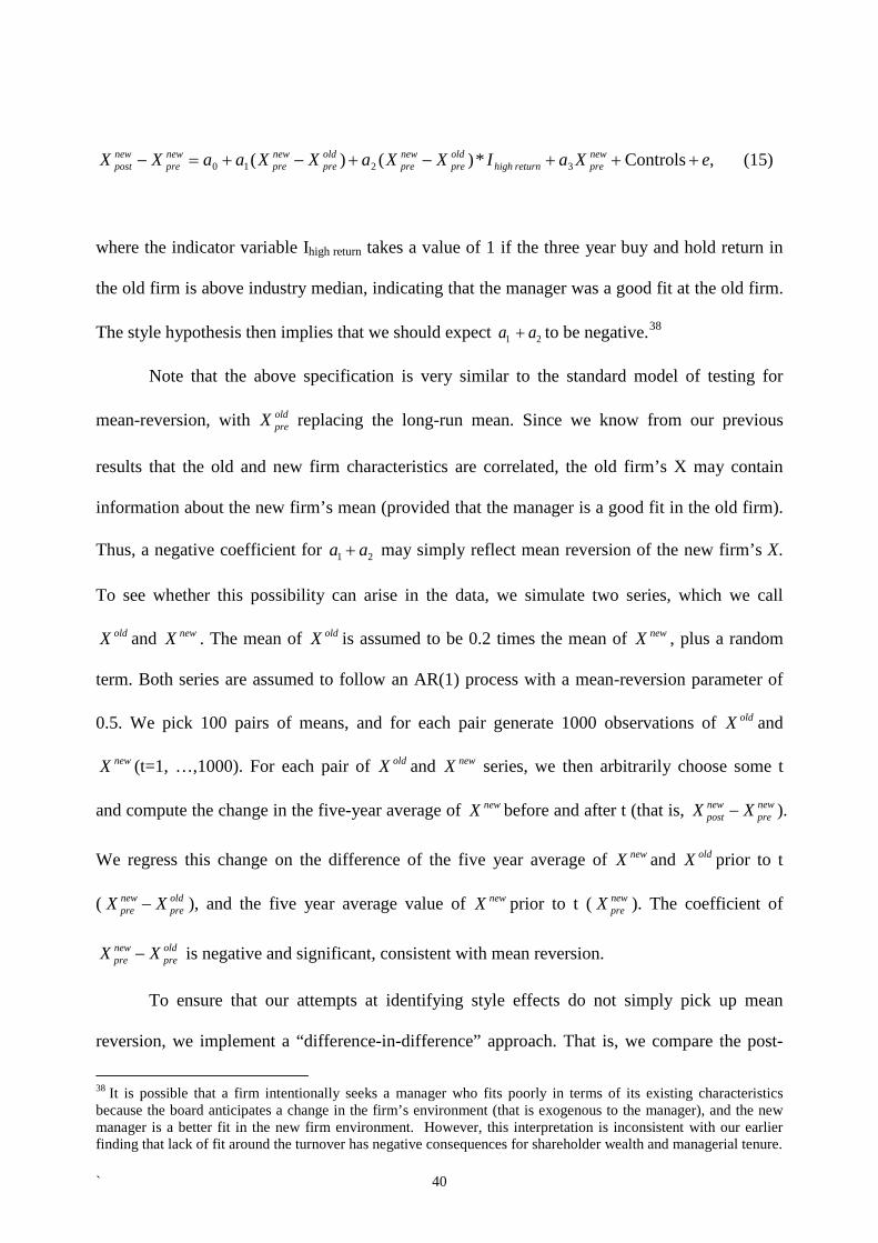
(15) , Controls *)()( 3 210 eXaIXXaXXaaXX newprereturnhigh
oldpre
newpre
oldpre
newpre
newpre
newpost +++−+−+=−
where the indicator variable Ihigh return takes a value of 1 if the three year buy and hold return in
the old firm is above industry median, indicating that the manager was a good fit at the old firm.
The style hypothesis then implies that we should expect 21 aa + to be negative.38
Note that the above specification is very similar to the standard model of testing for
mean-reversion, with oldpreX replacing the long-run mean. Since we know from our previous
results that the old and new firm characteristics are correlated, the old firm’s X may contain
information about the new firm’s mean (provided that the manager is a good fit in the old firm).
Thus, a negative coefficient for 1 2a a+ may simply reflect mean reversion of the new firm’s X.
To see whether this possibility can arise in the data, we simulate two series, which we call
oldX and newX . The mean of oldX is assumed to be 0.2 times the mean of newX , plus a random
term. Both series are assumed to follow an AR(1) process with a mean-reversion parameter of
0.5. We pick 100 pairs of means, and for each pair generate 1000 observations of oldX and
newX (t=1, …,1000). For each pair of oldX and newX series, we then arbitrarily choose some t
and compute the change in the five-year average of newX before and after t (that is, new newpost preX X− ).
We regress this change on the difference of the five year average of newX and oldX prior to t
( new oldpre preX X− ), and the five year average value of newX prior to t ( new
preX ). The coefficient of
new oldpre preX X− is negative and significant, consistent with mean reversion.
To ensure that our attempts at identifying style effects do not simply pick up mean
reversion, we implement a “difference-in-difference” approach. That is, we compare the post-
38 It is possible that a firm intentionally seeks a manager who fits poorly in terms of its existing characteristics because the board anticipates a change in the firm’s environment (that is exogenous to the manager), and the new manager is a better fit in the new firm environment. However, this interpretation is inconsistent with our earlier finding that lack of fit around the turnover has negative consequences for shareholder wealth and managerial tenure.
` 40

turnover impact of the old firm characteristics with that during periods when there is not a
turnover. In other words, we use the level of 21 aa + during “normal” times as a benchmark.
Thus we have the following model:
(17) , Controls )(
(16) , Controls *)()(''
3'
1'0
''
3 210
eXaXXaaXX
eXaIXXaXXaaXXnewpre
oldpre
newpre
newpre
newpost
newprereturnhigh
oldpre
newpre
oldpre
newpre
newpre
newpost
+++−+=−
+++−+−+=−’’
where in Equation (16) the pre- and post- periods are defined relative to t, the turnover year,
while in Equation (17), the pre-and-post variables for the new firm are defined relative to t-6, i.e.,
six years prior to the turnover year t. Each equation is applied to one cross-section of data. If
style matters, we expect 21 aa + to be significantly more negative than ’1a . As in earlier tests,
pre- and post-X are all five year average values of X. high returnI is an indicator variable for three-
year buy and hold returns at the old firm being above the industry median. “Controls” include
the high return indicator and the five year average value of the log of market value of the new
firm.
We estimate equations (16)-(17) in nested form, that is, we combine the two equations by
creating an indicator variable turnoverI indicating whether “pre” and “post” refer to the turnover
year t, or year t-6. We then interact this indicator variable with
.*)( and )( returnhigholdpre
newpre
oldpre
newpre IXXXX −− More specifically, we use the below model:
(18) , Controls **)(
*)()('3 2
1'10
eXaIIXXb
IXXbXXaaXXnewpreturnoverreturnhigh
oldpre
newpre
turnoveroldpre
newpre
oldpre
newpre
newpre
newpost
+++−+
−+−+=−
` 41

We expect 21 bb + to be significantly negative. In Table 9, we report the regression results for
which 21 bb + is negative. 39 It turns out 21 bb + is significantly negative for intangibles,
advertising expenditures, goodwill, acquisitions, beta, illiquidity, and the book-to-market ratio.
In tests not reported in the Table, we further split oldpre
newpre XX − into positive and negative
values. For goodwill and acquisitions, 21 bb + is significantly negative irrespective of the sign of
oldpre
newpre XX − , while intangibles and illiquidity are negatively significant for negative values of
oldpre
newpre XX − and negative but marginally insignificant for positive values. For Beta, b1 + b2 is
negatively significant only for negative values of the difference, whereas for advertisement, b1 +
b2 is negatively significant only for positive vales of the difference.
These results suggest that acquisition activity is one of the major manifestations of
managerial style, and managers who previously managed firms exposed to more systematic risk
tend to increase the systematic risk of the new firms they move to. Similarly, managers who
previously managed “growth” firms (low book-to-market) tend to move new firms in the same
direction. Stock liquidity in new firms tends to improve when they bring in managers from firms
that are more liquid (we have consistent evidence from the share turnover regression, although
for this variable, 21 bb + is not significant overall).
Other than share turnover, a few other variables that do not have significant values for
21 bb + for the overall sample have significant effects either for positive values or negative
values of oldpre
newpre XX − . ROA and OROA both have negative significant coefficients (at 5% and
10% levels, respectively) for positive values of oldpre
newpre XX − . This suggests that when managers
at firms with weaker operating performance (but above industry median stock returns) move to
firms with better performance, the effect is to weaken the operating performance of the latter.
39 We do not report the estimates of '1a in Table 9. In 9 out of 32 regressions, this coefficient has a negative sign
significant at least at the 5% level; in 16 regressions, the coefficient is negative and the t-statistic is above 1.4. The coefficient is positive in 5 regressions, but only one is marginally significant.
` 42

Cash holding also has a negative significant coefficient when oldpre
newpre XX − is positive. The ratio
of systematic risk to total risk, similar to beta, has a significant coefficient only for negative
values of oldpre
newpre XX − . Interestingly, for capital expenditure, we find that 21 bb + is negative and
significant for positive values of oldpre
newpre XX − but positive and significant for negative values of
oldpre
newpre XX − , suggesting that capital expenditure on average decreases at the new firm.
Overall, these results suggest the presence of managerial style effects. It is interesting to
note that several of the variables that appear to be affected due to misfit belong to our list of
match-relevant variables and the “mismatch” measure, e.g., acquisitions, beta, and the book-to-
market ratio (turnover and the ratio of market to total risk also feature for negative values
of oldpre
newpre XX − . This is exactly what we should expect if managerial attributes that match with
these characteristics are considered important.
6. Conclusion
In recent assignment models, equilibrium entails positive assortative matching between
firms and managers based on firm size and managerial talent. Managerial “ability” or “talent” is
seen in these models as essentially a one-dimensional attribute over which all firms have the
same preference ordering (i.e., all firms prefer a more talented manager). A closely related
notion is that “general” management skills have become more important in recent decades and
these skills are readily portable from one firm to another. Some have argued that the escalation
in top management pay is a direct consequence of improvements in managerial mobility and
improvement in managers’ outside options due to the greater importance of general management
skills.
In contrast, in this paper, we find strong evidence for the notion that assignment depends
on fit between firms and managers along multiple dimensions, which implies that firms with
different characteristics value managerial attributes differently. This suggests that competition
` 43

for managers may be much more limited because firms with different characteristics need
managers with specific attributes that fit these characteristics. In other words, the market for
managerial talent is much more segmented than generally assumed. How multi-dimensional
matching or fit affects equilibrium assignment and the allocative efficiency of managerial talent
should be major issues for future research. Recent papers by Edmans and Gabaix (2011) and
Eisfeldt and Kuhnen (2013) represent important steps in this direction.
` 44
References
Allgood, S. and K. A. Farrell, 2003, The Match between CEO and Firm, Journal of Business 76, 317–341. Amihud, Y., 2002 Illiquidity and Stock Returns: Cross-Section and Time-Series Effects, Journal of Financial Markets 5, 31-56 Bandiera, O., L. Guiso, A. Prat, and R. Sadun, 2012, Matching Firms, Managers, and Incentives, CEP Discussion Paper No.1144. Banerjee, S., S. Dasgupta and Y. Kim, 2008, Buyer-Supplier Relationships and the Stakeholder Theory of Capital Structure, Journal of Finance 63 (5), 2507-2552. Bennedsen, M., F. Pérez-González, and D. Wolfenzon, 2010, Do CEOs Matter? Working Paper, Columbia Business School. Bertrand, M., A. Schoar, 2003, Managing with Style: The Effect of Managers on Firm Policies, Quarterly Journal of Economics 118, 1169-1208. Brennan, M. J., T. Chordia and A. Subrahmanyam, 1998, Alternative Factor Specifications, Security Characteristics and the Cross-Section of Expected Stock Returns, Journal of Financial Economics 49, 345-373. Cen, L., S. Dasgupta, K. Chan and N. Gao, 2012, When the Tail Wags the Dog: Industry Leaders, Limited Attention, and Spurious Cross-Industry Information Diffusion, forthcoming, Management Science. Chang, Y., S. Dasgupta, and G. Hillary, 2010, CEO Ability, Pay, and Firm Performance, Management Science 56, 1633-1652. Edmans, A. and X. Gabaix, 2011, The Effect of Risk on the CEO Market, Review of Financial Studies 24, 2822-2863. Eisfeldt, A. L., and C. M. Kuhnen, 2013, CEO Turnover in a Competitive Assignment Framework, forthcoming, Journal of Financial Economics. Falato, A., D. Li, and T. Milbourn, 2013, Which Skills Matter in the Market for CEOs? Evidence from Pay for CEO Credentials, Working Paper. Fama, E.F. and K.R. French, 1997, Industry Costs of Equity, Journal of Financial Economics 43, 153-193. Fee, C. E., C. J. Hadlock, and J. R. Pierce, 2013, Managers With and Without Style: Evidence using Exogenous Variation, Review of Financial Studies 26(3), 567-601. Frydman, C., 2007, Rising Through the Ranks: The Evolution of the Market for Corporate Executives, 1936-2003, Working paper Frydman, C., and R.E. Saks, 2010, Executive Compensation: A New View from a Long-Term Perspective, 1936-2005, Review of Financial Studies 23, 2099-2138.
` 45

Gabaix, X., A. Landier, 2008, Why Has CEO Pay Increased So Much? Quarterly Journal of Economics 123 49-100. Graham, J. R., C. R. Harvey, and M. Puri, 2012, Managerial Attitudes and Corporate Actions, forthcoming, Journal of Financial Economics.
Graham, John, Si Li and Jiaping Qiu, 2011, Managerial Attributes and Executive Compensation, Review of Financial Studies 24, 1944-1979.
Groysberg, B., A. N. McLean, and N. Nohria, May 2006, Are Leaders Portable? Harvard Business Review 84, 92-100. Kaplan, S., M. Klebanov, and M. Sorensen, 2012, Which CEO Characteristics and Abilities Matter? Journal of Finance 67, 973-1007. Kothari, S.P.., A. J. Leone and C. E. Wasley, 2005, Performance Matched Discretionary Accrual Measures, Journal of Accounting and Economics 39, 163-197. Malmendier, U, and G. Tate, 2005, CEO Overconfidence and Corporate Investment, Journal of Finance 60, 2661-2700. Murphy, K. J. and J. Zábojník, 2004, CEO Pay and Appointments: A Market-Based Explanation for Recent Trends, American Economic Review 94(2), 192–196. Murphy, K. J. and J. Zábojník, 2007, Managerial Capital and the Market for CEOs, SSRN Working paper. Nguyen, B.D., K.M. Nielsen, 2010, What Death Can Tell: Are Executives Paid for Their Contributions to Firm Value? AFA 2011 Denver Meetings Paper. Pan, Y., 2012, The Determinants and Impact of Executive-Firm Matches, Working Paper, University of Utah. Rosen, S., 1974, Hedonic Prices and Implicit Markets: Product Differentiation in Pure Competition, Journal of Political Economy 82, 34–35. Rosen, S., 1981, The Economics of Superstars, American Economic Review 71(5), 845–858. Sattinger, M., 1979, Differential Rents and the Distribution of Earnings, Oxford Economic Papers 31, 60–71. Sattinger, M., 1993, Assignment Models of the Distribution of Earnings, Journal of Economic Literature 31, 831–880. Terviö, M., 2008, The Difference that CEOs Make: An Assignment Model Approach, American Economic Review 98(3), 642-668.
` 46

Appendix 2: Construction of Variables 1. Acquisitions
Acquisitions (aqc) over the beginning-of-period book value of assets (lagged at) = aqc/lagged at
2. Advertising Expenditures Advertising expenditures (xad) over the beginning-of-period total assets (lagged at) = xad/lagged at
3. Assets (Book Assets) = at
4. Beta The estimated slope coefficient of the following regression: Rj,t - Rf,t = interceptj + slopej*(Rm,t - Rf,t) + ej,t (A2)
5. Book-to-market Ratio = ceq/(prc*csho) where ceq is the book value of common equity; prc is the closing share price of the fiscal year; csho is the common share outstanding.
6. Business-Segment Herfindahl-Hirschman Index:
∑ ∑
s ssales
sales2
where s indexes business segments
7. Capital Expenditures
Capital expenditures (capx) over net property, plant, and equipment at the beginning of the fiscal year (lagged ppent) = capx/lagged ppent
8. Cash Holdings Cash and short-term investment (che) over net property, plant, and equipment at the beginning of the fiscal year (lagged ppent) = che/lagged ppent
9. Cash Flow The sum of earnings before extraordinary items (ib) and depreciation (dp) over net property, plant, and equipment at the beginning of the fiscal year (lagged ppent) = (ib+dp)/lagged ppent
10. Discretionary Accruals (Kothari, Leone and Wasley, 2005) The discretionary accruals is the residual value of the following regression.
TAit = a0 + a1(1/ASSETSit-1) + a2(∆SALESit) + a3 PPEit + a4 OIBDPit-1 + eit (A3) where i indexes firms; t indexes years; TA = (∆Data4 - ∆Data1 - ∆Data5 + ∆Data34 – Data14)/Lagged Data 6; ∆SALES = ∆Data12, scaled by Lagged Data 6; PPE = Data8 scaled by Lagged Data 6; OIBDP is the operating income before depreciation scaled by total assets. The regression is run cross-sectionally each year using all firm-year observations in the same two-digit SIC code.
` 47

• data4; ACT: current assets • data1; CHE: cash and short-term investments • data5; LCT: current liabilities • data34; DLC: debt in current liabilities • data14; DP: depreciation and amortization • data12; SALE: net sales • data8; PPENT: net PPE • data6; AT: total assets
11. Dividends
Dividends over earnings = (dvc+dvp)/oibdp where dvc is dividends for common equity; dvp is dividends for preferred shares; oibdp is operating income before depreciation.
12. Excess Return Over Market The annual stock return minus the annual market return
13. Geographical Segment Herfindahl-Hirschman Index:
∑ ∑
s ssales
sales2
where s indexes geographical segments
14. Goodwill
Goodwill (gdwl) over total assets (at) = gdwl/at
15. Idiosyncratic Risk Residual sum of squares from the following regression:
Rj,t - Rf,t = interceptj + slopej*(Rm,t - Rf,t) + ej,t (A2)
16. Illiquidity:
∑=
jD
d dj
dj
j VOLR
D 1
1,
,
where Rj,d is the daily return on stock j on day d, VOLj,d is the daily trading volume for stock j on day d, and Dj is the number of days with data in a year (Amihud (2002)).
17. Intangibles/Assets: Intangible assets (intan) over total assets (at) = intan/at
18. Interest Coverage Earnings before depreciation, interest, and tax (oibdp) over interest expenses (xint) = oibdp/xint
19. Leverage Long-term debt (dltt) plus debt in current liabilities (dlc) over long-term debt plus debt in current liabilities plus the book value of common equity (ceq) = (dltt+dlc)/(dltt+dlc+ceq)
` 48

20. Market Value
The book value of assets (at) plus the market value of common equity (prc×csho) less the sum of the book value of common equity (ceq) and balance sheet deferred taxes (txdb) = at+prc×csho–(ceq+txdb)
21. Non-Discretionary Accruals (Kothari, Leone and Wasley, 2005) The non-discretionary accruals is the predicted value of the following regression.
TAit = a0 + a1(1/ASSETSit-1) + a2(∆SALESit) + a3 PPEit + a4 OIBDPit-1 + eit (A3) where i indexes firms; t indexes years; TA = (∆Data4 - ∆Data1 - ∆Data5 + ∆Data34 – Data14)/Lagged Data 6; ∆SALES = ∆Data12, scaled by Lagged Data 6; PPE = Data8 scaled by Lagged Data 6; OIBDP is the operating income before depreciation scaled by total assets. The regression is run cross-sectionally each year using all firm-year observations in the same two-digit SIC code.
• data4; ACT: current assets • data1; CHE: cash and short-term investments • data5; LCT: current liabilities • data34; DLC: debt in current liabilities • data14; DP: depreciation and amortization • data12; SALE: net sales • data8; PPENT: net PPE • data6; AT: total assets
22. Price-to-earnings Ratio
= prc/epsfx where prc is the closing share price of the fiscal year; epsfx is earnings per share (diluted) excluding extraordinary items
23. ROA Income before extraordinary items (ib) over the beginning-of-period total assets (lagged at) = ib/lagged at
24. R&D Expenditures R&D expenditures (xrd) over the beginning-of-period total assets (lagged at) = xrd/lagged at
25. Operating ROA Operating net cash flow (oancf) over the beginning-of-period total assets (lagged at)
= oancf/lagged at
26. Sales over Assets (Vertical Integration) = sale/lagged at
27. Selling, General, and Administrative Expense Selling, general and administrative expense (xsga) over the beginning-of-period sales (lagged sale) = xsga/lagged sale
28. Systematic Risk/Total Risk (R2) R2 from the following regression:
Rj,t - Rf,t = interceptj + slopej*(Rm,t - Rf,t) + ej,t (A2)
` 49

29. Trading Volume
The average of daily dollar trading volume over a year (Brennan, Chordia, and Subrahmanyam (1998)).
30. Tobin’s Q Market Value divided by Assets. Both Market Value and Assets are defined above.
31. Turnover
The average of daily share turnover over a year, where the daily share turnover is calculated as the number of shares traded in a day divided by the number of shares outstanding as of the end of that day.
` 50

Table 1. Sample Statistics
“New firm” refers to the firm the manager joins, and “old firm” refers to the firm the manager leaves. Panel A reports the median and mean ratio of the new firm's market value/book assets (in 2000 dollars), as of the year prior to the appointment, to the old firm's market value/book assets (in 2000 dollars), as of the year prior to the departure; the number of observations; the percent of CEO-to-CEO moves, non-CEO-to-CEO moves and CEO-to-non-CEO moves in the sample. Panel B presents the means and medians of firm characteristics for three groups of firms for the period 1987-2009 that are examined in the paper. The construction of these characteristics is given in Appendix 2. Superscripts ***, ** and * indicate that the statistic is significantly different from that of the new firm at 1%, 5% and 10%, respectively. Superscripts a, b and c indicate that the statistic is significantly different from that of the largest 1500 in terms of market value of Compustat/CRSP at 1%, 5% and 10%, respectively.
Panel A: New vs. Old Size
CEO-to-CEO Moves Non-CEO-to-CEO
Moves CEO-to-Non-CEO Moves
Median Mean Median Mean Median Mean
Market Value: New Firm/Old Firm 1.79 5.46 0.2 0.56 2.71 7.86
Book Assets: New Firm/Old Firm 2.02 6.06 0.19 0.82 1.49 7.05
Frequency Percent Frequency Percent Frequency Percent
Number of Observations 171 0.44 188 0.49 27 0.07
` 51
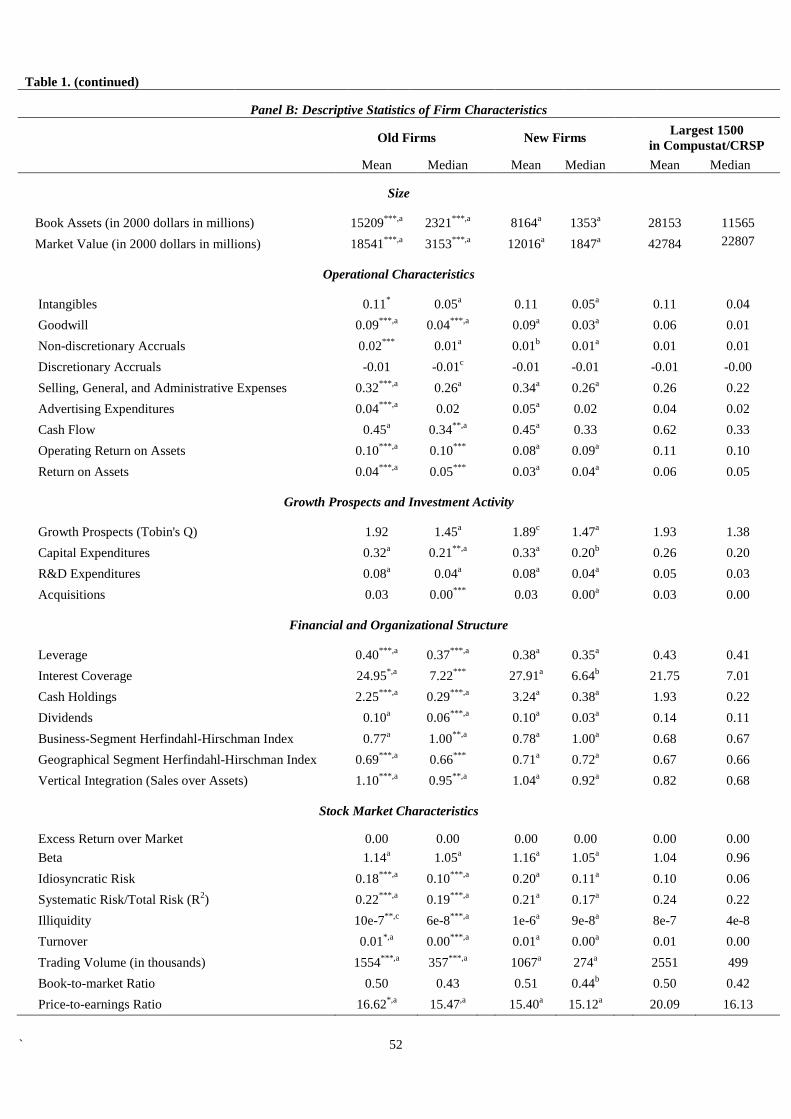
Table 1. (continued)
Panel B: Descriptive Statistics of Firm Characteristics
Old Firms New Firms Largest 1500 in Compustat/CRSP
Mean Median Mean Median Mean Median
Size
Book Assets (in 2000 dollars in millions) 15209***,a 2321***,a 8164a 1353a 28153 11565 Market Value (in 2000 dollars in millions) 18541***,a 3153***,a 12016a 1847a 42784 22807
Operational Characteristics
Intangibles 0.11* 0.05a 0.11 0.05a 0.11 0.04 Goodwill 0.09***,a 0.04***,a 0.09a 0.03a 0.06 0.01 Non-discretionary Accruals 0.02*** 0.01a 0.01b 0.01a 0.01 0.01 Discretionary Accruals -0.01 -0.01c -0.01 -0.01 -0.01 -0.00 Selling, General, and Administrative Expenses 0.32***,a 0.26a 0.34a 0.26a 0.26 0.22 Advertising Expenditures 0.04***,a 0.02 0.05a 0.02 0.04 0.02 Cash Flow 0.45a 0.34**,a 0.45a 0.33 0.62 0.33 Operating Return on Assets 0.10***,a 0.10*** 0.08a 0.09a 0.11 0.10 Return on Assets 0.04***,a 0.05*** 0.03a 0.04a 0.06 0.05
Growth Prospects and Investment Activity
Growth Prospects (Tobin's Q) 1.92 1.45a 1.89c 1.47a 1.93 1.38 Capital Expenditures 0.32a 0.21**,a 0.33a 0.20b 0.26 0.20 R&D Expenditures 0.08a 0.04a 0.08a 0.04a 0.05 0.03 Acquisitions 0.03 0.00*** 0.03 0.00a 0.03 0.00
Financial and Organizational Structure
Leverage 0.40***,a 0.37***,a 0.38a 0.35a 0.43 0.41 Interest Coverage 24.95*,a 7.22*** 27.91a 6.64b 21.75 7.01 Cash Holdings 2.25***,a 0.29***,a 3.24a 0.38a 1.93 0.22 Dividends 0.10a 0.06***,a 0.10a 0.03a 0.14 0.11 Business-Segment Herfindahl-Hirschman Index 0.77a 1.00**,a 0.78a 1.00a 0.68 0.67 Geographical Segment Herfindahl-Hirschman Index 0.69***,a 0.66*** 0.71a 0.72a 0.67 0.66 Vertical Integration (Sales over Assets) 1.10***,a 0.95**,a 1.04a 0.92a 0.82 0.68
Stock Market Characteristics
Excess Return over Market 0.00 0.00 0.00 0.00 0.00 0.00 Beta 1.14a 1.05a 1.16a 1.05a 1.04 0.96 Idiosyncratic Risk 0.18***,a 0.10***,a 0.20a 0.11a 0.10 0.06 Systematic Risk/Total Risk (R2) 0.22***,a 0.19***,a 0.21a 0.17a 0.24 0.22 Illiquidity 10e-7**,c 6e-8***,a 1e-6a 9e-8a 8e-7 4e-8 Turnover 0.01*,a 0.00***,a 0.01a 0.00a 0.01 0.00 Trading Volume (in thousands) 1554***,a 357***,a 1067a 274a 2551 499 Book-to-market Ratio 0.50 0.43 0.51 0.44b 0.50 0.42 Price-to-earnings Ratio 16.62*,a 15.47,a 15.40a 15.12a 20.09 16.13
` 52

Table 2. Summary Statistics of Decile Rank Distance (DRD) Between Characteristics of Old and New Firms Each year, for firms in Compustat/CRSP, we sort each firm characteristic into deciles and assign decile ranks (1=largest and 10=smallest). We then calculate the absolute difference of the rank of the characteristic of the old firm as of the year after the move and that of the new firm as of the year before the move (DRD). We also calculate the average of the absolute difference in rank of all 29 variables (ADRD). For the latter, missing variables are ignored in computing the average. The table reports the mean, 25, 50 and 75 percentiles of the absolute difference in ranks. Match-relevant Variable mean p25 p50 p75
ADRA (all variables combined) 2.28 1.72 2.14 2.72
Decile Rank Distance (DRD) Panel A: Size
Market Value 1.27 0 1 2 Book Assets 1.46 0 1 2
Panel B: Operational Characteristics Intangibles 1.89 1 2 3 Goodwill 1.62 1 1 2 Non-discretionary Accruals 2.72 1 2 4 Discretionary Accruals 2.63 1 2 4 Selling, General, and Administrative Expenses 1.92 1 2 3 Advertising Expenditures 2.11 1 2 3 Cash Flow 2.39 1 2 3 Return on Assets 2.46 1 2 4 Operating Return on Assets 2.42 1 2 4
Panel C: Growth Prospects and Investment Activities Tobin's Q 2.39 1 2 4 Capital Expenditures 2.30 1 2 3 R&D Expenditures 1.38 0 1 2 Acquisitions 1.09 0 1 2
Panel D: Financial and Organizational Structure Leverage 2.77 1 1 4 Interest Coverage 2.42 1 2 4 Cash Holdings 2.18 1 2 3 Dividends 1.30 0 1 2 Business Segment Herfindahl-Hirschman Index 2.21 1 2 4 Geographical Segment Herfindahl-Hirschman Index 1.85 1 2 3 Vertical Integration (Sales over Assets) 1.83 1 1 3
Panel E: Stock Market Characteristics Excess Return over Market 2.99 1 3 5 Beta 2.59 1 2 4 Idiosyncratic Risk 2.31 1 2 3 Systematic Risk/Total Risk 2.75 1 2 4 Illiquidity 1.47 0 1 2 Trading Volume 1.67 0 1 3 Turnover 2.08 1 2 3 Book-to-market Ratio 2.59 1 2 4 Price-to-earnings Ratio 2.51 1 2 4
` 53
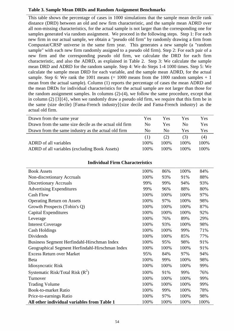
Table 3. Sample Mean DRDs and Random Assignment Benchmarks
This table shows the percentage of cases in 1000 simulations that the sample mean decile rank distance (DRD) between an old and new firm characteristic, and the sample mean ADRD over all non-missing characteristics, for the actual sample is not larger than the corresponding one for samples generated via random assignment. We proceed in the following steps. Step 1: For each new firm in our actual sample, we obtain a "pseudo old firm" by randomly drawing a firm from Compustat/CRSP universe in the same firm year. This generates a new sample (a "random sample" with each new firm randomly assigned to a pseudo old firm). Step 2: For each pair of a new firm and the corresponding pseudo old firm, we calculate the DRD for each firm characteristic, and also the ADRD, as explained in Table 2. Step 3: We calculate the sample mean DRD and ADRD for the random sample. Step 4: We do Steps 1-4 1000 times. Step 5: We calculate the sample mean DRD for each variable, and the sample mean ADRD, for the actual sample. Step 6: We rank the 1001 means (= 1000 means from the 1000 random samples + 1 mean from the actual sample). Column (1) reports the percentage of cases the mean ADRD and the mean DRDs for individual characteristics for the actual sample are not larger than those for the random assignment samples. In columns (2)-(4), we follow the same procedure, except that in column (2) [3]{4}, when we randomly draw a pseudo old firm, we require that this firm be in the same (size decile) [Fama-French industry]{size decile and Fama-French industry} as the actual old firm.
Drawn from the same year Yes Yes Yes Yes Drawn from the same size decile as the actual old firm No Yes No Yes Drawn from the same industry as the actual old firm No No Yes Yes (1) (2) (3) (4) ADRD of all variables 100% 100% 100% 100% ADRD of all variables (excluding Book Assets) 100% 100% 100% 100%
Individual Firm Characteristics
Book Assets 100% 86% 100% 84% Non-discretionary Accruals 100% 93% 91% 88% Discretionary Accruals 99% 99% 94% 93% Advertising Expenditures 99% 96% 88% 80% Cash Flow 100% 100% 100% 97% Operating Return on Assets 100% 97% 100% 98% Growth Prospects (Tobin's Q) 100% 100% 100% 87% Capital Expenditures 100% 100% 100% 92% Leverage 100% 76% 89% 29% Interest Coverage 100% 93% 100% 98% Cash Holdings 100% 100% 99% 71% Dividends 100% 100% 85% 77% Business Segment Herfindahl-Hirschman Index 100% 95% 98% 91% Geographical Segment Herfindahl-Hirschman Index 100% 100% 100% 91% Excess Return over Market 95% 84% 97% 94% Beta 100% 99% 100% 98% Idiosyncratic Risk 100% 100% 100% 99% Systematic Risk/Total Risk (R2) 100% 91% 99% 76% Turnover 100% 100% 100% 99% Trading Volume 100% 100% 100% 99% Book-to-market Ratio 100% 99% 100% 78% Price-to-earnings Ratio 100% 97% 100% 98% All other individual variables from Table 1 100% 100% 100% 100%
54

Table 4. Regression Results on the Relationship Between Characteristics of the "New" and "Old" Firms with Finer Industry and Size Control
This table reports the regression coefficient estimates of the following models: Xold
post = α0 + α1Xnewpre + eold
post (T1) Xold
post = β0 + β1 Xnewpre + β2 Xnew
pre*IndustryMatch + β3 Xnewpre*SizeMatch + eold
post (T2) where Xold
post is the average value of X of the old firm over the 5 years after the manager leaves the old firm. Xnewpre is the average
value of X of the new firm over the 5 years before the manager joins the new firm. IndustryMatch takes a value of 1 if the new firm's Fama-French 48 industry classification is the same as that of the old firm, and 0 otherwise. SizeMatch takes a value of 1 if the new and old firms have the same size decile rank, and 0 otherwise. t statistics are based on robust standard errors using the Huber-White sandwich estimators. ***, ** and * denote 1%, 5% and 10% level of significance, respectively. # indicates 10% significance level for a two-sided test. R2 and N (the number of observations) are those of the model (1).
α1 N R2 β1 β2 β3 Panel A: Size
Log(Market Value) 0.435*** 162 0.18 0.301*** -0.014 0.134*** Log(Book Assets) 0.353*** 219 0.17 0.276*** -0.002 0.118***
Panel B: Operational Characteristics
Intangibles 0.304*** 190 0.07 0.383*** -0.465*** -0.006 Goodwill 0.304*** 162 0.07 0.348*** -0.306* -0.104 Discretionary Accruals 0.346*** 179 0.04 0.356* -0.213 0.553** Cash Flow 0.069* 204 0.00 0.050 0.028 -0.006 Operating Return on Assets 0.203** 205 0.07 0.029 0.277** 0.038
Panel C: Growth Prospects and Investment Activities
Growth Prospects (Tobin's Q) 0.227*** 162 0.06 0.258** -0.098 0.002 R&D Expenditures 0.174* 114 0.13 0.222*** -0.071 0.092 Capital Expenditures 0.218* 199 0.14 0.253* -0.112 -0.180 Acquisitions 0.307* 189 0.04 0.438* -0.259** -0.305
Panel D: Financial and Organizational Structure
Cash Holdings 0.097** 209 0.01 0.114# -0.014 -0.040 Leverage 0.189*** 216 0.04 0.118# 0.096 0.057 Dividends 0.234*** 209 0.06 0.099# 0.197* 0.280*** Vertical Integration (Sales over Assets) 0.343*** 218 0.10 0.269*** 0.210** -0.182**
Panel E: Stock Market Characteristics
Beta 0.246*** 189 0.08 0.272*** -0.054 -0.053 Idiosyncratic Risk 0.151* 189 0.03 0.064 0.163 -0.240 Market Risk/Total Risk (R2) 0.313*** 189 0.06 0.300*** -0.099 0.096 Turnover 0.312*** 189 0.09 0.255*** 0.136 -0.065 Log(Trading Volume) 0.449*** 189 0.18 0.428*** -0.015 0.045*** Book-to-market Ratio 0.182* 197 0.03 0.168# 0.052 0.011
55

Table 5. Regression Results on the Relationship Between Characteristics of the "New" and "Old" Firms with Coarser Industry and Size Control
This table reports the regression coefficient estimates of the following models: Xold
post = β’0 + β’1 Xnew
pre + β’2 Xnewpre*IndustryMatch2 + β’3 Xnew
pre*SizeMatch2 + eoldpost (T3)
where Xoldpost is the average value of X of the old firm over the 5 years after the manager leaves the old
firm. Xnewpre is the average value of X of the new firm over the 5 years before the manager joins the new
firm. IndustryMatch2 takes a value of 1 if the new firm and the old firm are classified in the same Fama-French 48 industry or 2-digit SIC industry, and 0 otherwise. SizeMatch2 takes a value of 1 if the new firm is in the same or an adjacent size decile rank as that of the old firm, and 0 otherwise. t statistics are based on robust standard errors using the Huber-White sandwich estimators. ***, ** and * denote 1%, 5% and 10% level of significance, respectively. # indicates 10% significance level for a two-sided test. R2 and N (the number of observations) are those of the model (1). β’1 β’2 β’3
Panel A: Size Log(Market Value) 0.289*** -0.031 0.131*** Log(Book Assets) 0.325*** 0.000 0.050*
Panel B: Operational Characteristics Intangibles 0.378*** -0.346** 0.001 Goodwill 0.314*** -0.337** 0.118 Discretionary Accruals 0.290# -0.138 0.353 Cash Flow 0.047 0.031 0.000 Operating Return on Assets 0.077 0.261** -0.133
Panel C: Growth Prospects and Investment Activities Growth Prospects (Tobin's Q) 0.206* -0.094 0.093 R&D Expenditures 0.134 0.000 -0.015 Capital Expenditures 0.268*** -0.115 -0.017 Acquisitions 0.567# -0.356*** -0.343
Panel D: Financial and Organizational Structure Cash Holdings 0.116# -0.015 -0.018 Leverage 0.123# 0.077 0.050 Dividends 0.089 0.259** 0.107 Vertical Integration (Sales over Assets) 0.246*** 0.216** -0.018
Panel E: Stock Market Characteristics Beta 0.316*** -0.025 -0.124* Idiosyncratic Risk 0.114# 0.124 -0.080 Market Risk/Total Risk (R2) 0.349*** -0.114 0.004 Turnover 0.220** 0.122 0.122 Log(Trading Volume) 0.448*** -0.022 0.014 Book-to-market Ratio 0.186# 0.034 -0.101
56

Table 6. Summary of Main Results in Tables 4 and 5: Variables Relevant for Firm-Manager Matching ("Match-Relevant Variables") + indicates a significant and positive estimated coefficient of Xnew
pre in Table 4 or Table 5; a blank cell indicates an insignificant estimated coefficient of Xnew
pre. Controlling for Industry Match and Size Match NO (α1) YES (β1) YES (β’1)
Panel A: Size
Market Value + + +
Book Assets + + + Panel B: Operational Characteristics
Intangibles + + +
Goodwill + + +
Discretionary Accruals + +
Cash Flow +
Operating Return on Assets + Panel C: Growth Prospects and Investment Activities
Growth Prospects (Tobin's Q) + + + R&D Expenditures + + Capital Expenditures + + +
Acquisitions + + Panel D: Financial and Organizational Structure
Cash Holdings + Leverage + Dividends +
Vertical Integration (Sales over Assets) + + + Panel E: Stock Market Characteristics
Idiosyncratic Risk + Beta + + + Market Risk/Total Risk (R2) + + +
Turnover + + +
Trading Volume + + +
Book-to-market Ratio +
57
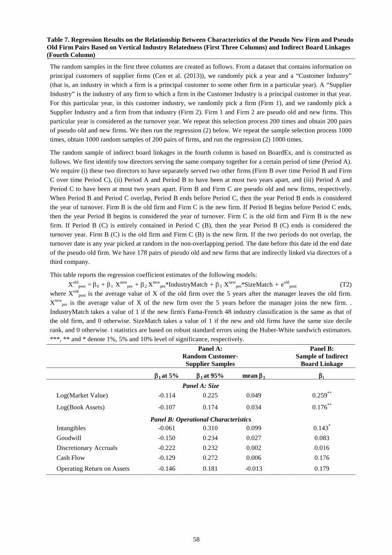
Table 7. Regression Results on the Relationship Between Characteristics of the Pseudo New Firm and Pseudo Old Firm Pairs Based on Vertical Industry Relatedness (First Three Columns) and Indirect Board Linkages (Fourth Column) The random samples in the first three columns are created as follows. From a dataset that contains information on principal customers of supplier firms (Cen et al. (2013)), we randomly pick a year and a “Customer Industry” (that is, an industry in which a firm is a principal customer to some other firm in a particular year). A “Supplier Industry” is the industry of any firm to which a firm in the Customer Industry is a principal customer in that year. For this particular year, in this customer industry, we randomly pick a firm (Firm 1), and we randomly pick a Supplier Industry and a firm from that industry (Firm 2). Firm 1 and Firm 2 are pseudo old and new firms. This particular year is considered as the turnover year. We repeat this selection process 200 times and obtain 200 pairs of pseudo old and new firms. We then run the regression (2) below. We repeat the sample selection process 1000 times, obtain 1000 random samples of 200 pairs of firms, and run the regression (2) 1000 times.
The random sample of indirect board linkages in the fourth column is based on BoardEx, and is constructed as follows. We first identify tow directors serving the same company together for a certain period of time (Period A). We require (i) these two directors to have separately served two other firms (Firm B over time Period B and Firm C over time Period C), (ii) Period A and Period B to have been at most two years apart, and (iii) Period A and Period C to have been at most two years apart. Firm B and Firm C are pseudo old and new firms, respectively. When Period B and Period C overlap, Period B ends before Period C, then the year Period B ends is considered the year of turnover. Firm B is the old firm and Firm C is the new firm. If Period B begins before Period C ends, then the year Period B begins is considered the year of turnover. Firm C is the old firm and Firm B is the new firm. If Period B (C) is entirely contained in Period C (B), then the year Period B (C) ends is considered the turnover year. Firm B (C) is the old firm and Firm C (B) is the new firm. If the two periods do not overlap, the turnover date is any year picked at random in the non-overlapping period. The date before this date id the end date of the pseudo old firm. We have 178 pairs of pseudo old and new firms that are indirectly linked via directors of a third company.
This table reports the regression coefficient estimates of the following models: Xold
post = β0 + β1 Xnewpre + β2 Xnew
pre*IndustryMatch + β3 Xnewpre*SizeMatch + eold
post (T2) where Xold
post is the average value of X of the old firm over the 5 years after the manager leaves the old firm. Xnew
pre is the average value of X of the new firm over the 5 years before the manager joins the new firm. . IndustryMatch takes a value of 1 if the new firm's Fama-French 48 industry classification is the same as that of the old firm, and 0 otherwise. SizeMatch takes a value of 1 if the new and old firms have the same size decile rank, and 0 otherwise. t statistics are based on robust standard errors using the Huber-White sandwich estimators. ***, ** and * denote 1%, 5% and 10% level of significance, respectively.
Panel A: Random Customer- Supplier Samples
Panel B: Sample of Indirect
Board Linkage
β1 at 5% β1 at 95% mean β1
β1
Panel A: Size Log(Market Value) -0.114 0.225 0.049 0.259**
Log(Book Assets) -0.107 0.174 0.034 0.176**
Panel B: Operational Characteristics Intangibles -0.061 0.310 0.099 0.143* Goodwill -0.150 0.234 0.027 0.083 Discretionary Accruals -0.222 0.232 0.002 0.016 Cash Flow -0.129 0.272 0.006 0.176 Operating Return on Assets -0.146 0.181 -0.013 0.179
58

Table 7. (Continued)
Panel A: Random Customer-
Supplier Samples
Panel B: Sample of Indirect
Board Linkage
β1 at 5% β1 at 95% mean β1
β1
Panel C: Growth Prospects and Investment Activities Growth Prospects (Tobin's Q) -0.099 0.263 0.025 -0.034**
R&D Expenditures -0.244 0.315 0.003 0.937* Capital Expenditures -0.102 0.125 0.003 0.031 Acquisitions -0.105 0.160 0.006 0.010
Panel D: Financial and Organizational Structure Cash Holdings -0.082 0.259 0.019 0.068 Leverage -0.129 0.151 -0.002 0.010 Dividends -0.127 0.133 -0.001 0.073 Vertical Integration (Sales over Assets) -0.115 0.201 0.045 -0.042
Panel E: Stock Market Characteristics Beta -0.191 0.243 0.012 -0.001 Idiosyncratic Risk -0.237 0.266 -0.008 -0.013
Market Risk/Total Risk (R2) -0.218 0.296 0.018 0.168** Turnover -0.075 0.656 0.233 -0.129**
Log(Trading Volume) 0.060 0.538 0.298 0.201* Book-to-market Ratio -0.146 0.230 0.025 0.043
59

Table 8. Match Quality: Effects on Shareholder Wealth, Managerial Pay and Tenure This table presents regression results on how the quality of the manager's match at the new firm affects the stock price reaction of the new firm to the appointment news, the managerial pay and tenure at the new firm. The dependent variable in columns (1) and (2) is the cumulative abnormal return from the day before to the day after the announcement day of the managerial appointment, and in columns (3) and (4) it is the natural logarithm of the manager's total pay in the year after the appointment year in the new firm. In columns (5) and (6), we estimate the departure rate at the new firm based on the Cox model, where we exclude cases in which the manager leaves the firm because the firm no longer exists. We create an indicator for the observations with high pre-departure 3-year stock return for the old firm (above the industry median) and another indicator for the observations with low pre-departure 3-year stock return for the old firm (below the industry median). We interact each explanatory variable separately with these two indicators. Mismatch is constructed as follows. We consider 7 "match-relevant" variables: Tobin's Q, acquisition, sales/assets, turnover, beta, systematic risk/total risk (R2), and book-to-market ratio. For each of these variables, we create an indicator that takes a value of 1 if the decile rank distance between the new and the old firm is at least one standard deviation from the mean of all of the event firm pairs, and 0 otherwise. Mismatch is the sum of the 7 indicators. Low Info of the prior new firm is the residual from the regression where we regress the reciprocal of the idiosyncratic risk, based on the daily returns of the new firm over the year before the appointment, on log(market value), Fama-French industry dummies, year dummies, interactions of Fama-French industry dummies and year dummies. Low Info Dummy takes a value of 1 when the Low Info is in the top 25 percentile, and 0 otherwise. Industry Mismatch takes a value of 1 if the old and new firms are in different industries (based on Fama-French 48 industry classification), and 0 otherwise. Size Mismatch takes a value of 1 if the absolute rank difference in size between the old and new firms is larger than 1, and 0 otherwise. Log(market value) is the natural logarithm of the market value of the new firm as of the year prior to the executive appointment. Leverage is long-term debt plus debt in current liabilities over long-term debt plus debt in current liabilities plus the book value of common equity of the new firm as of the year prior to the manager's appointment. Prior Tenure is the length of tenure (in days) of the manager in the old firm. Past Stock Return is the stock return of the new firm for the year prior to the manager's appointment. Industry Past Stock Return is the corresponding industry median of Past Stock Return. Industry and year fixed effects are included in columns (3)-(4). The table reports the estimated coefficients of the ordinary least squares linear regressions [in columns (1)-(4)] or the "hazard ratio" of the Cox regression [in columns (5)-(6)], corresponding absolute t or z statistics (in parentheses), based on robust standard errors for all columns, Adjusted R2 or Wald Chi Square , and the number of observations. ***, ** and * denote 1%, 5% and 10% level of significance, respectively.
60

Dependent Variable: Appointment CAR log(Total Pay) Tenure
(1) (2) (3) (4) (5) (6)
High Pre-departure 3-year Stock Return for the Old Firm
Intercept 0.083** 0.085* 15.515*** 15.682*** (2.00) (1.89) (4.22) (4.30) Mismatch -0.019** -0.019** -0.255** -0.261** 1.256*** 1.317*** (2.07) (2.01) (2.00) (2.05) (3.50) (3.93) Mismatch*Low Info Dummy -0.032* -0.031* (1.89) (1.81) Low Info -0.001 -0.001 (0.45) (0.45) Industry Mismatch -0.014 0.049 0.634** (0.73) (0.26) (1.98) Size Mismatch 0.006 0.067 1.373 (0.35) (0.35) (1.57) log(Market Value) -0.006 -0.005 0.359*** 0.362*** 1.021 1.029 (1.06) (0.97) (5.55) (5.16) (0.38) (0.53) Leverage 0.046 0.048 -0.157 -0.182 0.978 0.973 (1.41) (1.42) (0.52) (0.62) (0.63) (0.72) Prior Tenure 0.999 1.000
(1.28) (1.43)
Past Stock Return 1.025 1.084 (0.38) (0.96) Industry Past Stock Return 0.597 0.526 (1.04) (1.31)
61

Dependent Variable: Appointment CAR log(Total Pay) Tenure
(1) (2) (3) (4) (5) (6)
Low Pre-departure 3-year Stock Return for the Old Firm Intercept -0.054 -0.055 2.255 3.484 (1.58) (1.43) (0.72) (1.09) Mismatch 0.008 0.008 0.137 0.108 1.034 1.050 (0.95) (0.92) (1.28) (1.01) (0.28) (0.42) Mismatch*Low Info Dummy 0.006 0.006 (0.58) (0.51) Low Info -0.002 -0.002 (1.49) (1.48) Industry Mismatch 0.000 -0.422 0.670 (0.00) (1.66) (1.19) Size Mismatch 0.003 0.130 0.674 (0.18) (0.61) (1.44) log(Market Value) 0.006 0.006 0.434*** 0.452*** 0.965 0.987 (1.47) (1.45) (4.49) (4.46) (0.40) (0.15) Leverage 0.022 0.022 -0.690* -0.838** 0.796 0.660 (0.83) (0.78) (1.89) (2.25) (0.36) (0.58) Prior Tenure 1.000 1.000 (0.34) (0.05) Past Stock Return 0.909 0.933 (1.21) (1.21) Industry Past Stock Return 0.618 0.502 (0.85) (1.15)
Adjusted R2 0.112 0.096 0.586 0.582 Wald Chi Square 22.89** 31.22** Number of Observations 217 217 181 181 207 207
62

Table 9. Testing for Style
This table reports the regression coefficient estimates for Equation (18) in the main body of the paper:
(18) , Controls **)(
*)()('3 2
1'1
'0
eXaIIXXb
IXXbXXaaXXnewpreturnoverreturnhigh
oldpre
newpre
turnoveroldpre
newpre
oldpre
newpre
newpre
newpost
+++−+
−+−+=−
where turnoverI equals one if pre- and post- are calculated based on the turnover year and zero if pre- and
post- are calculated based on the non-turnover year t-6. Both pre- and post- are the five-year average values with respect to the reference year. The model is the nested form of Equations (16) and (17) in the paper. returnhighI is an indicator variable for three-year buy and hold returns at the old firm being above the
industry median. Controls include the high return indicator and the five year average value of the log of market value of the new firm. t statistics are based on robust standard errors using the Huber-White sandwich estimators. ***, ** and * denote 1%, 5% and 10% level of significance, respectively. N is the number of observations used in the regression.
b1 b1+b2 N R2
Panel A: Operational Characteristics
Intangibles -0.082 -0.196** 291 0.10 Goodwill -0.074 -0.232** 200 0.10 Advertising Expenditures 0.045 -0.374** 66 0.56
Panel B: Growth Prospects and Investment Activities
Acquisitions -0.049 -0.292*** 309 0.57
Panel E: Stock Market Characteristics
Beta -0.058 -0.312** 322 0.36 Illiquidity -1.00*** -1.717* 323 0.58 Book-to-market Ratio 0.045 -0.305* 328 0.32
63
Top Related