


Languages
Pages
Legal


Robust Parameter Designwith Feed-Forward Control
V. Roshan Joseph
School of Industrial and Systems Engineering
Georgia Institute of Technology
Atlanta, GA 30332-0205
Accepted by Technometrics.
Abstract
When there exists strong noise factors in the process, robust parameter design alone
may not be effective and a control strategy can be used to compensate for the effect of
noise. In this article, a parameter design methodology in the presence of a feed-forward
control is developed. In particular, performance measures for evaluating control factor
settings in measurement systems, simple response systems, and multiple target systems
are developed. Strategies for the design and analysis of experiments are discussed. The
approach is illustrated using an example on gold plating.
KEY WORDS: Experiments, Optimization, Process control, Quality engineering.
1

1. INTRODUCTION
Robust parameter design attempts to make the process insensitive to noise by appropri-
ately choosing levels for the control factors. Pioneered by Taguchi (1987) robust parameter
design has been recognized as an important tool for quality improvement. See Wu and
Hamada (2000), Wu and Wu (2000), and Vuchkov and Boyadjieva (2001) for the recent
developments. The robustness is achieved by exploiting the control-by-noise interactions.
Consider the following example, suppose the response y at time t follows the model
yt = 10 + 2x1 − qt − 0.5rt + x2rt + εt, (1)
where (x1, x2) are the control factors and (q, r) the noise factors, and ε is the random error
caused by the other noise factors in the process. For simplicity, let q, r, and ε be independent
with mean 0 and variance 1. Suppose initially the process was set at (x1, x2) = (0,−1) to
achieve the target 10 on average which results in a variance of 4.25. The robust parameter
design solution is to change the setting of x2 to 0.5. We see that by this change the effect of
r on y is removed. Thus the variance of y reduces to 2. Because q does not interact with x1
or x2, the approach cannot reduce/eliminate the variations caused by this noise factor. In
such cases tolerance design is often used as a remedy measure. In this example the tolerance
of q will be tightened so as to reduce the variation in y to a desired level.
An alternative approach is to compensate for the effect of noise. For example, we can
adjust x1 depending on q using the control law x1t = 0.5qt, so that the effect of q on
y is eliminated. Now the variation in y reduces to 1. This approach can be effectively
implemented if q is on-line measurable and x1 is on-line adjustable.
From the above discussions it is clear that the robust parameter design solution works
only if there exists control-by-noise interactions. The control solution does not require any
such conditions and therefore has a much wider applicability. But the control solution needs
on-line measurements of the noise and a controller to implement the control law. This
increases the cost of production. Moreover unlike robust parameter design this is not a
one-time activity and requires continuous monitoring and maintenance. Therefore it is not
2

prudent to jump into control systems without investigating the opportunities for robustness.
A cost-effective strategy would be to use robust parameter design to make the process as
robust as possible and then use a control system or tolerance design approach to further
improve the process.
A two-stage approach for quality improvement using first robust parameter design and
then control systems may not always work well. For example in (1) if V ar(ε) = (1 + x1x2)2,
then the robust parameter design solution will depend on the control law and vice versa. In
such cases we cannot decouple the methodology into two stages and arrive at the optimal
solution.
In many processes there exists strong noise which cannot be de-sensitized by parameter
design. The use of control systems is inevitable in such cases. When such noise factors are
known a priori, the experiments are designed and the optimization is carried out so that the
control law becomes robust to the other noise factors. Taguchi and his co-workers call such
experiments as double-signal experiments. See, for example, Fowlkess and Creveling (1995,
Section 6.5) and Wu and Wu (2000, Chapter 4). Many real case studies can be found in
Taguchi, Chowdhury, and Taguchi (2000, Chapters 4, 9, 14, and 18). The case studies are
quite successful, albeit using rudimentary modeling and optimization techniques.
In this article we develop a general methodology for robust parameter design of systems
with control. The article is organized as follows. In Section 2 we explain the application
of control in the optimization of measurement systems. The connection with the signal-
to-noise ratio analysis is established. In Section 3 we develop the optimization procedure
for feed-forward control in the simple response systems. The robust parameter design of
multiple target systems with feed-forward control is discussed in Section 4. The approach
is illustrated using an example on gold plating in Section 5. Some concluding remarks and
future research directions are given in Section 6.
3

2. MEASUREMENT SYSTEMS
Taguchi, Chowdhury, and Taguchi (2000, Chapter 4) reports a case study on the accuracy
improvement of a disposable oxygen sensor used for open heart surgery. The sensor is used
for measuring the oxygen concentration in the blood. There are several control factors
for this measurement system such as sensor thickness, polymer molecular weight, dye-to-
polymer ratio, over coat size and type, etc. There are several noise factors such as time
at elevated temperature, exposure to ambient light, sensor thickness variation, etc. The
blood temperature is also a noise factor because it varies from operation to operation. It is
possible to continuously measure the blood temperature and give a feed-forward correction
using an algorithm in the monitor’s software. This experiment is different from the usual
robust parameter design experiments because no effort is made to de-sensitize the effect of
blood temperature on the measurements. The objective is to set the levels of the control
factors such that the oxygen concentration measurements become robust to the noise after
compensating for the effect of blood temperature.
We will first explain the robust parameter design without any control and then describe
it with control so that direct comparisons can be made. More details about measurement
systems without control can be found in Miller and Wu (1996) and Wu and Hamada (2000,
Chapter 11).
2.1 Without Control
Let M be the true value of the variable, Y the measured value, X the set of control
factors, and Z the set of noise factors. Assume that Y and M are nonnegative variables.
Let Y = f(X,Z,M). Suppose that there is no zero-correction required in the measurement
system, i.e., Y = 0 when M = 0. Then we can approximate the above relationship in the
operating range of M by
Y = β(X,Z)M. (2)
If the relationship is nonlinear, then adding an intercept term will improve the fit, but will
complicate the optimization. We will discuss the use of intercept term at the end of this
4

section.
Partition Z into {N,U} where N is the observable (or known) set of noise factors and U
the unobservable (or unknown) set of noise factors in the experiment. Let E[β(X,Z)|N] =
β(X,N) and V ar[β(X,Z)|N] = V (X,N). Because U is unobservable we may use the
following additive noise model
Y = β(X,N)M + ε, (3)
where E(ε|N) = 0 and V ar(ε|N) = V (X,N)M2. For the moment, we will assume that the
functions β and V are known to the experimenter and will derive the performance measures
for optimization. In real practice these functions are not known and are to be estimated from
the data by conducting experiments. We will consider the issue of estimation in Section 2.4.
From an observed value of Y , M can be estimated as
M =Y
E[β(X,N)]. (4)
Let E[β(X,N)] = β(X). Then the variation in the estimate is
V ar(M) =V ar(Y )
β2(X). (5)
The V ar(Y ) can be obtained as follows:
V ar(Y ) = E[V ar(Y |N)] + V ar[E(Y |N)]
= E[V (X,N)M2] + V ar[β(X,N)M ]
= σ2(X)M2,
where σ2(X) = E[V (X,N)] + V ar[β(X,N)]. Thus
V ar(M) =σ2(X)M2
β2(X).
Letting D be the feasible region for X, our objective is to find an X ∈ D to minimize the
variance of M . This can be done by maximizing the signal-to-noise (SN) ratio given by
SN(X) =β2(X)
σ2(X). (6)
5

Note that the V ar(M) is a function of M . In this particular case maximizing SN ratio
will minimize the variance for all the values of M . For some other models this need not be
the case and one may have to average the V ar(M) over the distribution of M to get the
performance measure. The approach can be summarized as follows
1. Find X∗ ∈ D to maximize SN(X) in (6).
2. Estimate M = Y/β(X∗).
It is pointed out that the SN ratio in (6) is different from Taguchi’s signal-to-noise
ratio, because the underlying modeling assumptions are different. Joseph and Wu (2002a,b)
has shown the validity of model (3) in multiple target systems and we adopt this for the
measurement systems.
Now consider a model with an intercept term. Let
Y = β0(X) + β1(X,N)M + ε,
where E(ε|N) = 0 and V ar(ε|N) = V (X,N)M2. We will continue to assume that the true
relationship between Y and M passes through the origin. The β0(X) is introduced to get a
better fit to the true model in the operating range of M . A reasonable estimator for M is
M = max
{0,
Y − β0(X)
β1(X)
},
where β1(X) = E[β1(X,N)]. Because of the nonlinearity in the estimator, obtaining an
explicit expression for the performance measure is difficult. But if P (Y ≤ β0(X)) is small
in the operating range of M , then we can take the estimator as M = (Y − β0(X))/β1(X).
Now the variance of M can be obtained as before. It is easy to show that the required
performance measure is the same as the SN ratio in (6) with β(X) replaced by β1(X).
2.2 With Control
We may not be able to compensate for all of the N in the usual operation of the system.
So divide N into {Q,R}, where we call Q the on-line noise factors and R the off-line
noise factors. The on-line noise factors can be easily measured and compensated during
6

the operation of the system. They have a large effect on the response, otherwise it is not
worthwhile to apply a compensation strategy on them. In the oxygen sensor example Q is the
blood temperature. The off-line noise factors are systematically varied in the experiment
but are unobserved during the operation of the system. The use of off-line noise factors
improves the efficiency of parameter design experiments. See the discussions in Berube and
Nair (1998) and Steinberg and Bursztyn (1998).
Consider the same model as in (3),
Y = β(X,Q,R)M + ε, (7)
where E(ε|Q,R) = 0 and V ar(ε|Q,R) = V (X,Q,R)M2. Because Q is on-line measurable,
a feed-forward correction will be applied based on the values of Q. A measurement system
with control is diagrammatically depicted in Figure 1. Feed-back control is not possible in
measurement systems, because the true value of the variable is not known during the usual
operation of the system.
M - β
?
X
- Y - 1/E(β) - M
6Z
6 6N U
6 6R Q
6
Figure 1: Measurement System with Control
Let E[β(X,Q,R)|Q] = β(X,Q). Assume that β(X,Q) > 0 with probability 1. Then
from an observed value of Y , M can be estimated as
M =Y
β(X,Q). (8)
Notice that unlike in (4), the slope in (8) is allowed to change with the values of the on-line
noise. To obtain the performance measure for optimization we need to compute the variance
7

of M . To do this we proceed as follows. First note that M is an unbiased estimator of M ,
because
E(M |Q) =E(Y |Q)
β(X,Q)=
E[β(X,Q,R)|Q]M
β(X,Q)= M. (9)
For a given value of Q the variance is
V ar(M |Q) =V ar(Y |Q)
β2(X,Q)=
σ2(X,Q)M2
β2(X,Q)(10)
because
V ar(Y |Q) = E[V ar(Y |Q,R)|Q] + V ar[E(Y |Q,R)|Q]
= E[V (X,Q,R)M2|Q] + V ar[β(X,Q,R)M |Q]
= σ2(X,Q)M2,
where σ2(X,Q) = E[V (X,Q,R)|Q] + V ar[β(X,Q,R)|Q].
Using (9) and (10) we have
V ar(M) = E[V ar(M |Q)] + V ar[E(M |Q)]
= E
[σ2(X,Q)M2
β2(X,Q)
]+ V ar[M ]
= E
[σ2(X,Q)
β2(X,Q)
]M2.
Call SN(X,Q) = β2(X,Q)/σ2(X,Q), the signal-to-noise ratio for a given value of Q. Thus
the variance of M can be minimized by minimizing E{1/SN(X,Q)} for all values of M . An
equivalent performance measure to maximize is
PM(X) = 1/E{1/SN(X,Q)}= 1/E
{E[V (X,Q,R)|Q] + V ar[β(X,Q,R)|Q]
E2[β(X,Q,R)|Q]
}(11)
The approach can be summarized as
1. Find X∗ ∈ D to maximize PM(X) in (11).
2. Estimate M = Y/β(X∗,Q).
8

The signal-to-noise ratio in (6) can be written as
SN(X) =E2[β(X,Q,R)]
E[V (X,Q,R)] + V ar[β(X,Q,R)]. (12)
Comparing with (11) we see that the performance measure for optimization with control is
different.
2.3 Design of Experiments
We can think of the whole approach as to evaluate the performance of a control system at
different levels of control factor settings and to choose a setting that optimizes a performance
measure of the system. Thus a cross array design between X and the other factors is
intuitively appealing. Let D(a) be the design for the factors a. Let D(a)⊗D(b) denotes the
cross array design between two sets of factors a and b, which means that all the runs in D(b)
are repeated at each run of D(a). Then the cross array for the robust parameter design of
measurement systems with control is given by
D(X)⊗D(R)⊗D(Q)⊗D(M). (13)
If the model in (7) is true, then we do not need to vary M in the experiment and the functions
β and V can be estimated from the data by conducting the experiments at some fixed value
of M . However, using a design for M with at least two levels will allow us to verify this
modeling assumption and to possibly explore more elaborate models. The case studies in
Taguchi, Chowdhury, and Taguchi (2000) follow the design of experiments in (13). Because
of crossing of many factors, such experiments are much larger than the usual experiments
without a control system. One approach to reduce the number of runs is to use the noise
factor compounding technique (Taguchi, 1987). Because on-line noise has a special meaning
in experiments with control systems, the compounding should be applied only on R and not
on Q. Another approach to reduce the number of runs is to use single arrays instead of cross
arrays. Here apart from the main effects we are interested in the interaction between the
control factors and the off-line noise. Therefore we may reduce the design in (13) to
D(X,R,Q)⊗D(M). (14)
9

See Wu and Hamada (2000) and Wu and Zhu (2003) for the optimal selection of single arrays.
Their design criterion may require some modification for the use in control systems because
of the presence of two types of noise factors. Among the two-factor interactions, control ×off-line noise interactions are most important. The control × on-line noise interactions and
the control × control interactions will take the second and third places. The interactions
among the noise factors are least important. The three-factor interaction control × control
× off-line noise should get the same importance as that of control × control interactions.
The experiment should be designed in such a way that the important effects are at least
estimable. This task is more challenging in control systems because of the different kinds of
factors.
If the experimenter is not sure before conducting the experiment which noise factors
are to be compensated, then (13) should be used for the experiment. This will enable
the experimenter to identify the on-line noise from the set of noise factors considered in the
experiment. When the noise factors are of the inner noise type (variations around the nominal
value of the factor), they need not be included in the experiment. This can considerably
reduce the run size of the experiment. See Vuchkov and Boyadjieva (2001) for a detailed
treatment of robust parameter design with inner noise. The example to be presented in
Section 5 is of this kind.
2.4 Estimation
Let yijklp be the measured value of the characteristic at Xi,Qj,Rk,Ml, and replicate
p. Let Y ′ = Y/M . Consider the model in (7). Assume that the errors are indepen-
dent and follow normal distribution. Then y′ijklp = β(Xi,Qj,Rk) + ε′ijklp, where ε′ijklp ∼N(0, V (Xi,Qj,Rk)). Express the β(X,Q,R) and log V (X,Q,R) as linear models in X, Q,
and R. An iterative algorithm for obtaining maximum likelihood estimates (MLE) is given
below.
1. Initialize β(Xi,Qj,Rk) = y′ijk.. = 1LP
∑Ll=1
∑Pp=1 y′ijklp .
2. Compute s2ijk = 1
LP
∑Ll=1
∑Pp=1{y′ijklp − β(Xi,Qj,Rk)}2, where β(Xi,Qj,Rk) is the
10

predicted value of β at Xi,Qj, and Rk. Using s2ijk as the response, estimate the
parameters in log V (X,Q,R) using a gamma generalized linear model (GLM) with log
link.
3. Fit y′ijklp ∼ β(Xi,Qj,Rk) using weighted least squares with weights 1/V (Xi,Qj,Rk),
where V (Xi,Qj,Rk) is the predicted value of V at Xi,Qj, and Rk.
4. Repeat steps 2 and 3 until convergence.
This gives the MLE of the two functions β(X,Q,R) and V (X,Q,R). By plugging them
in (11) we get the MLE of the performance measure. If LP = 1, then the algorithm needs
some modification. For this case start with step 3 by initializing V (Xi,Qj,Rk) = 1.
If one is uncertain about the mean model, then it is better to omit the iterations between
steps 2 and 3. By doing so we can avoid the transmission of modeling errors in the mean
model to the variance model. The maximum likelihood approach is known to under esti-
mate the variance function because it does not adjust for the loss of degrees of freedom for
estimating the mean function. Suppose n is the number of parameters in β(X,Q,R). Then
we can inflate the s2ijk in the step 2 by a factor IJKLP/(IJKLP − n) to reduce the bias.
This method produces approximate restricted maximum likelihood estimate (See McCullagh
and Nelder, 1989, Section 10.5). If the distribution of ε is unknown, then one can use an
extended quasi-likelihood criterion for estimating the parameters by specifying appropriate
link and variance functions .
The modeling approach used so far is known as response modeling (Wu and Hamada,
2000, Chapters 10 and 11). There is another type of modeling that is commonly used in
parameter design literature, which is known as performance measure modeling. The estima-
tion procedure for performance measure modeling is different and is discussed below. By
absorbing R into U we can reduce the model in (3) to
Y = β(X,Q)M + ε, (15)
where E(ε|Q) = 0 and V ar(ε|Q) = σ2(X,Q)M2. In contrast to response modeling, here β
and log σ2 are not expressed as linear models in X and Q. Instead they are directly estimated
11

at each combination of Xi and Qj. To emphasize this difference we will denote β(Xi,Qj)
by βij and σ2(Xi,Qj) by σ2ij. We have
βij = y′ij... and σ2ij =
1
KLP
K∑
k=1
L∑
l=1
P∑
p=1
(y′ijklp − βij)2.
Then ˆSN ij = β2ij/σ
2ij. If the levels of Q in the experiment can be considered as a represen-
tative sample from its distribution, then the performance measure in (11) can be estimated
as
ˆPM i =
1
J
J∑
j=1
1ˆSN ij
−1
. (16)
This shows that the performance measure for optimization in a measurement system with
control is the harmonic mean of the SN ratios estimated at each of the on-line noise factor
levels. The log PM can be expressed as a linear model in X and estimated using ordinary
least squares. We note that if one intends to use the performance measure modeling, then
the experimental design in (14) should not be used. Performance measure modeling requires
crossing of the on-line noise factors with the other factors. Therefore the design in (13) or a
design of the type D(X,R)⊗D(Q)⊗D(M) should be used.
The model in (15) makes sense only if R has random levels in the experiment, which
is not the case in most robust parameter design experiments. Therefore the performance
measure modeling will not be as statistically efficient as the response modeling approach.
Also the performance measure modeling needs a cross array design for the experiment,
whereas response modeling can be used with all kinds of designs. Although the response
modeling approach looks superior, the performance measure modeling has some advantages
in control systems. The response modeling requires explicit modeling of Q. Therefore any
modeling errors will be transmitted to (11) and may affect the result. In performance measure
modeling ˆPM i in (16) can be estimated without explicit modeling of on-line noise and
therefore is insensitive to modeling inaccuracies. Once the optimal solution X∗ is obtained,
more data can be collected keeping X fixed at X∗ and the response can be modeled with
respect to Q to obtain the control law. This approach is particularly useful when β has a
nonlinear relationship with Q.
12
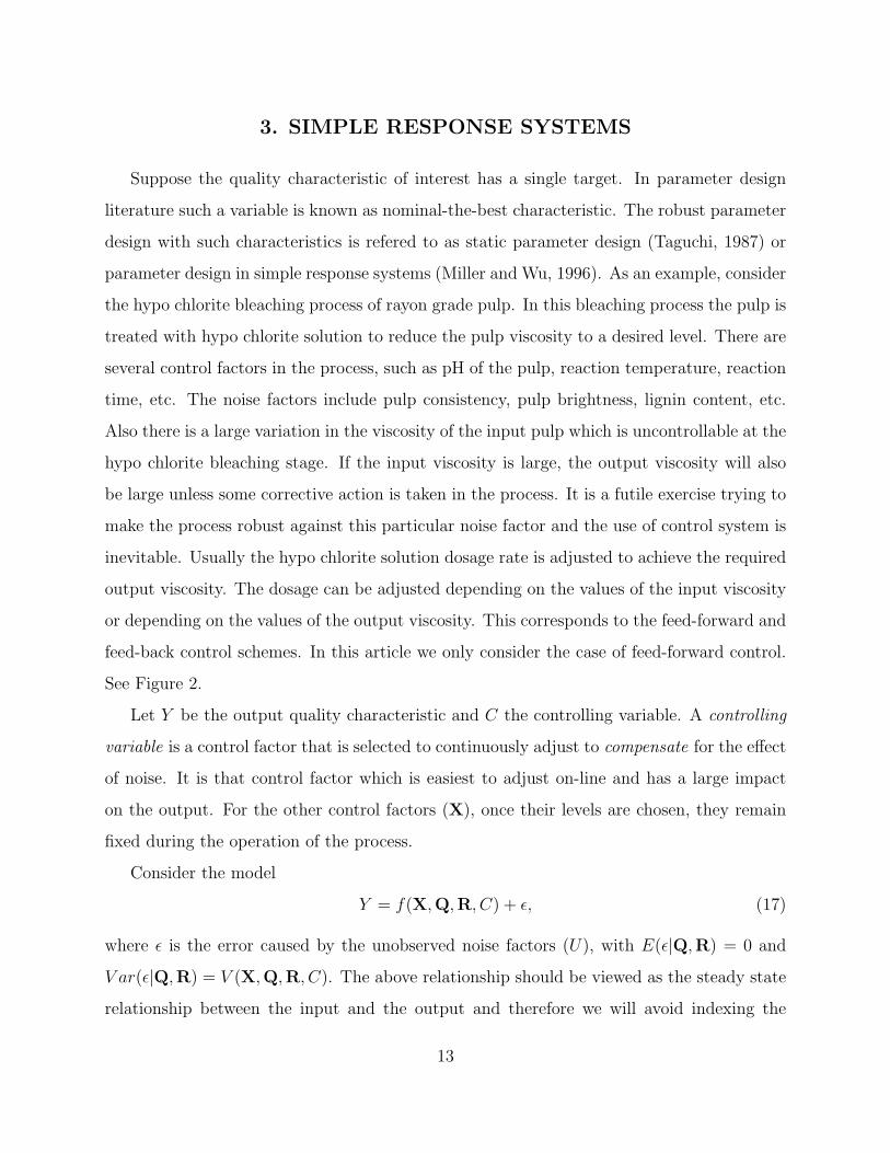
3. SIMPLE RESPONSE SYSTEMS
Suppose the quality characteristic of interest has a single target. In parameter design
literature such a variable is known as nominal-the-best characteristic. The robust parameter
design with such characteristics is refered to as static parameter design (Taguchi, 1987) or
parameter design in simple response systems (Miller and Wu, 1996). As an example, consider
the hypo chlorite bleaching process of rayon grade pulp. In this bleaching process the pulp is
treated with hypo chlorite solution to reduce the pulp viscosity to a desired level. There are
several control factors in the process, such as pH of the pulp, reaction temperature, reaction
time, etc. The noise factors include pulp consistency, pulp brightness, lignin content, etc.
Also there is a large variation in the viscosity of the input pulp which is uncontrollable at the
hypo chlorite bleaching stage. If the input viscosity is large, the output viscosity will also
be large unless some corrective action is taken in the process. It is a futile exercise trying to
make the process robust against this particular noise factor and the use of control system is
inevitable. Usually the hypo chlorite solution dosage rate is adjusted to achieve the required
output viscosity. The dosage can be adjusted depending on the values of the input viscosity
or depending on the values of the output viscosity. This corresponds to the feed-forward and
feed-back control schemes. In this article we only consider the case of feed-forward control.
See Figure 2.
Let Y be the output quality characteristic and C the controlling variable. A controlling
variable is a control factor that is selected to continuously adjust to compensate for the effect
of noise. It is that control factor which is easiest to adjust on-line and has a large impact
on the output. For the other control factors (X), once their levels are chosen, they remain
fixed during the operation of the process.
Consider the model
Y = f(X,Q,R, C) + ε, (17)
where ε is the error caused by the unobserved noise factors (U), with E(ε|Q,R) = 0 and
V ar(ε|Q,R) = V (X,Q,R, C). The above relationship should be viewed as the steady state
relationship between the input and the output and therefore we will avoid indexing the
13

C - System
?
X
- Y
6Z
6 6N U
6 6Q R
6
Figure 2: Simple Response System with Feed-Forward Control
variables with time t. As done in Section 2, we will assume that the functions f and V are
known and derive the performance measure. In practice these functions will be estimated
from the data and will be plugged-in to obtain the estimate of the performance measure.
The design of experiments will be similar to those discussed in Section 2.3 with M replaced
by C.
Let T be the target value of the quality characteristic. Suppose we use a quadratic loss
function to measure the quality of the output, L = (Y − T )2. Then the expected loss for
given Q and R is
E(L|Q,R) = (f(X,Q,R, C)− T )2 + V (X,Q,R, C).
Based on the observed value of Q, we can adjust the value of C to minimize the expected
loss averaged over the distribution of R given Q. This gives us the control law:
C∗ = arg minC
E[E(L|Q,R)|Q] = arg minC
E(L|Q). (18)
Thus C∗ is a function of X and Q. Let C∗ = h(X,Q). Cost considerations or system
limitations may require that the value of C be between CL and CH . In such cases the above
optimization should be performed by restricting C in [CL, CH ]. Now Q is a set of noise
factors and their variations during the operation of the process are uncontrollable. So we
will select an X to minimize the expected loss at C = C∗ taken over the distribution of Q.
14

Thus our objective is to find an X ∈ D to minimize
PM(X) = E(L∗) = E{E[L∗|Q]} = E{E[E(L∗|Q,R)|Q]} (19)
= E{E[(f(X,Q,R, h(X,Q))− T )2|Q]}+ E{E[V (X,Q,R, h(X,Q))|Q]}.
We call PM(X) a performance measure independent of control (PerMIC). This is an exten-
sion of the concept of performance measure independent of adjustment (PerMIA) to control
systems. See Leon, Shoemaker, and Kacker (1987) and Leon and Wu (1992) for details
on PerMIA. The PerMIC can be compared to a PerMIA by treating C as an adjustment
parameter. They are different because of the presence of on-line noise factors. It is easy to
show that
E(L∗) = E{minC
E(L|Q)} ≤ minC
E{E(L|Q)} = E(L∗o),
where E(L∗o) is the minimum expected loss without control. Here E(L∗) is a PerMIC and
E(L∗o) is a PerMIA. The above inequality shows that instituting a control system will improve
the performance of a system. But it is beneficial to use a control system only if the reduction
in the quality loss E(L∗o)− E(L∗) is much larger than the cost of implementing the control
system. The approach can be summarized as follows:
1. Find X∗ ∈ D to minimize PM(X) in (19).
2. Adjust C using the control law C = h(X∗,Q).
For on-line implementation, the control law will be written as Ct = h(X∗,Qt). This con-
trol law is obtained by assuming the model in (17). Therefore the control law is meaningful
only if the process is in a state of statistical control. If the process goes out-of-control due
to some special causes, the above control law may no longer be valid. Therefore statistical
process control techniques should be employed to check the stability of the process and to
take corrective actions (see, Montgomery, 2001).
To simplify the computations in (18) we may decide to adjust C to achieve the mean
of Y at target. In engineering such an unbiased adjustment strategy makes a lot of sense.
Then C∗ = h(X,Q), if exists, is a solution of C from
E[f(X,Q,R, C)|Q] = T. (20)
15
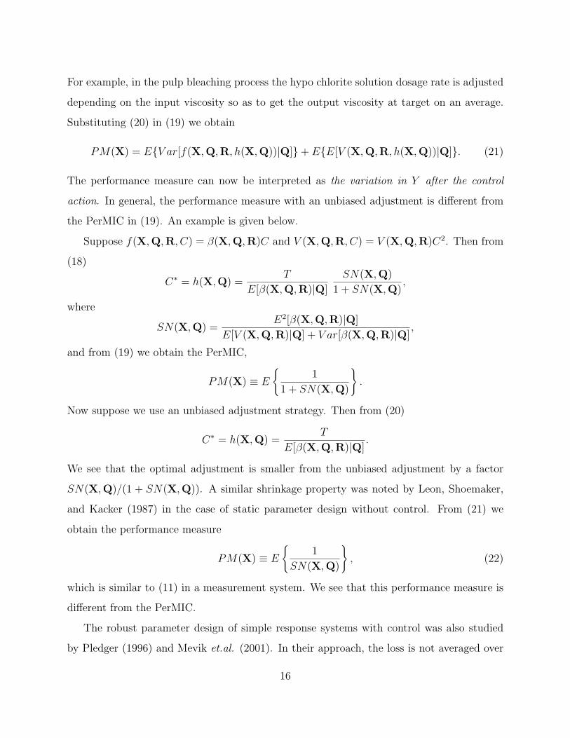
For example, in the pulp bleaching process the hypo chlorite solution dosage rate is adjusted
depending on the input viscosity so as to get the output viscosity at target on an average.
Substituting (20) in (19) we obtain
PM(X) = E{V ar[f(X,Q,R, h(X,Q))|Q]}+ E{E[V (X,Q,R, h(X,Q))|Q]}. (21)
The performance measure can now be interpreted as the variation in Y after the control
action. In general, the performance measure with an unbiased adjustment is different from
the PerMIC in (19). An example is given below.
Suppose f(X,Q,R, C) = β(X,Q,R)C and V (X,Q,R, C) = V (X,Q,R)C2. Then from
(18)
C∗ = h(X,Q) =T
E[β(X,Q,R)|Q]
SN(X,Q)
1 + SN(X,Q),
where
SN(X,Q) =E2[β(X,Q,R)|Q]
E[V (X,Q,R)|Q] + V ar[β(X,Q,R)|Q],
and from (19) we obtain the PerMIC,
PM(X) ≡ E
{1
1 + SN(X,Q)
}.
Now suppose we use an unbiased adjustment strategy. Then from (20)
C∗ = h(X,Q) =T
E[β(X,Q,R)|Q].
We see that the optimal adjustment is smaller from the unbiased adjustment by a factor
SN(X,Q)/(1 + SN(X,Q)). A similar shrinkage property was noted by Leon, Shoemaker,
and Kacker (1987) in the case of static parameter design without control. From (21) we
obtain the performance measure
PM(X) ≡ E
{1
SN(X,Q)
}, (22)
which is similar to (11) in a measurement system. We see that this performance measure is
different from the PerMIC.
The robust parameter design of simple response systems with control was also studied
by Pledger (1996) and Mevik et.al. (2001). In their approach, the loss is not averaged over
16

the on-line noise distribution to find X∗ and therefore X∗ is a function of Q. This approach
is difficult to implement in practice particularly when there are many control factors in the
system as all of them will have to be varied with the on-line noise. To overcome this situation
Berget and Naes (2002a,b) have proposed obtaining robust parameter design solution for
some specified categories and an optimal sorting for the raw materials (the on-line noise)
for selecting the categories. Our approach is different because only one control factor (C) is
selected from the set of control factors and varied with the on-line noise, which is the most
commonly used form of control in practice. The other control factors remain fixed at the
robust parameter design X∗. This is probably a better approach in continuous processes or
when there is too much of fluctuations in the on-line noise as only one factor need to be
adjusted frequently. However, in batch processes, one may consider using more than one
controlling variable.
4. MULTIPLE TARGET SYSTEMS
The optimization of multiple target systems (also known as dynamic parameter design)
comprises an important class of problems in robust parameter design. A detailed description
of it can be found in Miller and Wu (1996), Tsui (1999), and Joseph and Wu (2002a,b). As
an example, consider the injection molding process (Wu and Wu, 2000, page 102). Because
of the diversity of products, the products will have different dimensions. Depending on the
customer requirements, the different part dimensions can be achieved by changing the mold
dimensions. Fine adjustments to compensate for the various noise factors in the process
can be done through the injection pressure. Thus, here the mold dimension is the signal
factor (M) and the injection pressure is the controlling variable (C). In this article we only
consider the case of feed-forward control, see Figure 3.
Let
Y = f(X,Q,R,M,C) + ε, (23)
where E(ε|Q,R) = 0 and V ar(ε|Q,R) = V (X,Q,R,M, C). Suppose for a given customer
intent (T ) the loss is measured using the quadratic loss function, L = (Y − T )2. The
17

T©©*HHj
M -
C -System
?
X
- Y
6Z
6 6N U
6 6Q R
6
Figure 3: Multiple Target System with Feed-Forward Control
performance measure for multiple target systems without control is discussed in Joseph and
Wu (2002a,b). Using the concept of PerMIC this can be extended for multiple target systems
with control as
PM(X) =∫
E(L∗) dF (T ) =∫
minM
E{minC
E(L|Q)} dF (T )
=∫
E{(f(X,Q,R,M∗, C∗)− T )2}+ E{V (X,Q,R,M∗, C∗)} dF (T ), (24)
where F (T ) is the distribution of the customer intent. Thus we have the optimal control law
C∗ = arg minC
E(L|Q) (25)
and the optimal signal adjustment
M∗ = arg minM
E{minC
E(L|Q)}. (26)
Let C∗ = h(X,Q,M, T ) and M∗ = g(X, T ). The approach can be summarized as
1. Find X∗ ∈ D to minimize PM(X) in (24).
2. Adjust M depending on T as M = g(X∗, T ).
3. Adjust C depending on Q and T as C = h(X∗,Q, g(X∗, T ), T ).
18

In many systems there may not exist a unique solution to (25) and (26). In such cases
M∗ can be determined by fixing C at some value. Also the optimal adjustments in (25) and
(26) can be replaced by unbiased adjustments if they exist. We illustrate these situations
with two examples.
Example 1: Let f(X,Q,R,M, C) = β(X,Q,R)MC and V (X,Q,R,M, C) = V (X,Q,R)M2C2.
Clearly there is no unique solution to (25) and (26). Suppose [CL, CH ] is the preferred in-
terval for adjusting C. Then we will find the signal adjustment by fixing C at some value in
the interval, say, C0 = (CL + CH)/2. For unbiased adjustment
M∗ =T
C0E[β(X,Q,R)].
Again using unbiased adjustment for C, we obtain C∗ = T/E[β(X,Q,R)M |Q]. At M = M∗,
C∗ = C0E[β(X,Q,R)]
E[β(X,Q,R)|Q].
Note that here C∗ does not depend on T . The performance measure in (24) evaluated at
the above M∗ and C∗ becomes
PM(X) ≡ E
{E[V (X,Q,R)|Q] + V ar[β(X,Q,R)|Q]
E2[β(X,Q,R)|Q]
}= E
{1
SN(X,Q)
}, (27)
which is the as the same performance measure in (22). It is important to note that in this par-
ticular case we do not need to know the distribution of T to obtain the performance measure.
Example 2: In many systems, the signal factor and the controlling variable are the same.
For example, in an automobile, for the steering system the rotation of the steering wheel can
be used for both signal and control; for the braking system the force applied on the pedal can
be used for both signal and control. Such a factor can be represented as M + C, where M
denotes the initial adjustment to achieve the target and C represents the fine adjustments
of the factor around its initial value. Consider the following case: f(X,Q,R,M,C) =
β(X,Q,R)(M + C) and V (X,Q,R,M, C) = V (X,Q,R)(M + C)2. Here M should be
determined by fixing C = 0. Thus, for unbiased adjustments M∗ = T/E[β(X,Q,R)] and
19
C∗ = T/E[β(X,Q,R)|Q]− T/E[β(X,Q,R)]. The performance measure is the same as the
one in (27). It is pointed out that for automobiles, in practice, the driver will use feed-back
control for adjustments, a topic that is not developed in this article.
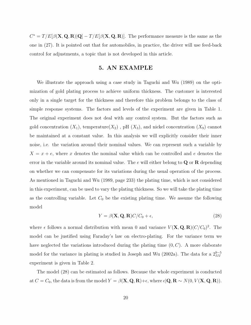
5. AN EXAMPLE
We illustrate the approach using a case study in Taguchi and Wu (1989) on the opti-
mization of gold plating process to achieve uniform thickness. The customer is interested
only in a single target for the thickness and therefore this problem belongs to the class of
simple response systems. The factors and levels of the experiment are given in Table 1.
The original experiment does not deal with any control system. But the factors such as
gold concentration (X1), temperature(X2) , pH (X3), and nickel concentration (X9) cannot
be maintained at a constant value. In this analysis we will explicitly consider their inner
noise, i.e. the variation around their nominal values. We can represent such a variable by
X = x + e, where x denotes the nominal value which can be controlled and e denotes the
error in the variable around its nominal value. The e will either belong to Q or R depending
on whether we can compensate for its variations during the usual operation of the process.
As mentioned in Taguchi and Wu (1989, page 233) the plating time, which is not considered
in this experiment, can be used to vary the plating thickness. So we will take the plating time
as the controlling variable. Let C0 be the existing plating time. We assume the following
model
Y = β(X,Q,R)C/C0 + ε, (28)
where ε follows a normal distribution with mean 0 and variance V (X,Q,R)(C/C0)2. The
model can be justified using Faraday’s law on electro-plating. For the variance term we
have neglected the variations introduced during the plating time (0, C). A more elaborate
model for the variance in plating is studied in Joseph and Wu (2002a). The data for a 29−5III
experiment is given in Table 2.
The model (28) can be estimated as follows. Because the whole experiment is conducted
at C = C0, the data is from the model Y = β(X,Q,R)+ε, where ε|Q,R ∼ N(0, V (X,Q,R)).
20
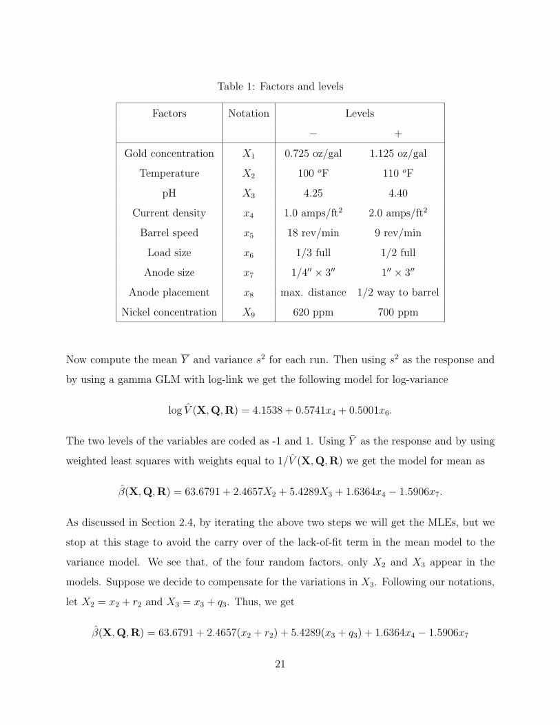
Table 1: Factors and levels
Factors Notation Levels
− +
Gold concentration X1 0.725 oz/gal 1.125 oz/gal
Temperature X2 100 oF 110 oF
pH X3 4.25 4.40
Current density x4 1.0 amps/ft2 2.0 amps/ft2
Barrel speed x5 18 rev/min 9 rev/min
Load size x6 1/3 full 1/2 full
Anode size x7 1/4′′ × 3′′ 1′′ × 3′′
Anode placement x8 max. distance 1/2 way to barrel
Nickel concentration X9 620 ppm 700 ppm
Now compute the mean Y and variance s2 for each run. Then using s2 as the response and
by using a gamma GLM with log-link we get the following model for log-variance
log V (X,Q,R) = 4.1538 + 0.5741x4 + 0.5001x6.
The two levels of the variables are coded as -1 and 1. Using Y as the response and by using
weighted least squares with weights equal to 1/V (X,Q,R) we get the model for mean as
β(X,Q,R) = 63.6791 + 2.4657X2 + 5.4289X3 + 1.6364x4 − 1.5906x7.
As discussed in Section 2.4, by iterating the above two steps we will get the MLEs, but we
stop at this stage to avoid the carry over of the lack-of-fit term in the mean model to the
variance model. We see that, of the four random factors, only X2 and X3 appear in the
models. Suppose we decide to compensate for the variations in X3. Following our notations,
let X2 = x2 + r2 and X3 = x3 + q3. Thus, we get
β(X,Q,R) = 63.6791 + 2.4657(x2 + r2) + 5.4289(x3 + q3) + 1.6364x4 − 1.5906x7
21

Table 2: Data of gold plating experiment
Run X1X9x4X2x7x8x5X3x6 Gold plating thickness in micro inches
1 −−−−−−−−− 63 52 57 60 51 64 57 56 61 57 58 51 54 60 54 64 50 54 55 49
2 −−−−+ + + + + 59 60 63 61 58 66 53 63 57 61 61 60 73 81 59 62 68 53 60 72
3 −−+ +−−−+ + 60 66 78 83 64 76 89 106 68 78 52 86 91 69 71 57 73 96 83 60
4 −−+ + + + +−− 67 77 66 51 53 55 59 58 62 62 81 76 60 58 53 59 55 54 70 60
5 −+−+−−+−+ 71 74 78 63 62 67 47 69 49 58 54 80 71 67 62 47 51 66 57 49
6 −+−+ + +−+− 70 58 69 65 65 74 71 75 75 65 70 64 65 66 55 70 71 74 65 75
7 −+ +−−−+ +− 61 66 65 74 66 73 73 65 83 81 60 75 77 62 60 69 65 60 89 76
8 −+ +−+ +−−+ 68 62 54 51 43 59 57 64 53 52 48 58 46 46 47 42 51 48 50 44
9 +−+−−+ +−+ 66 47 67 56 55 56 49 53 39 54 42 46 66 89 42 68 61 46 92 58
10 +−+−+−−+− 48 63 69 60 89 81 63 53 68 76 53 67 66 68 69 65 89 67 74 70
11 +−−+−+ + +− 75 76 75 70 71 70 84 68 75 73 80 76 69 71 70 75 67 68 76 66
12 +−−+ +−−−+ 58 55 47 49 59 45 53 56 41 53 61 52 55 55 54 50 53 52 56 55
13 + + + +−+−−− 64 65 57 76 54 54 65 60 64 67 62 62 67 57 67 58 55 61 64 56
14 + + + + +−+ + + 45 79 77 72 71 99 50 74 77 74 72 96 75 89 98 77 41 77 96 75
15 + +−−−+−+ + 84 53 56 64 61 74 57 56 69 65 72 57 48 64 64 67 55 68 56 55
16 + +−−+−+−− 61 60 55 50 54 51 50 56 57 55 53 52 57 52 53 52 54 55 55 49
22

and
V (X,Q,R) = exp(4.1538 + 0.5741x4 + 0.5001x6).
Assume that q3 and r2 follow normal distributions with means 0 and variances σ23 = (.05/.075)2 =
0.4444 and σ22 = (2/5)2 = 0.16 respectively. From (22) we have
ˆPM(X) = E
{exp(4.1538 + .5741x4 + .5001x6) + 2.46572σ2
2
(63.6791 + 2.4657x2 + 5.4289(x3 + q3) + 1.6364x4 − 1.5906x7)2
}.
We want to minimize ˆPM(X) with each variable restricted in the interval [−1, 1]. Using
Lemma 1 given in Appendix, we immediately get x∗2 = 1, x∗3 = 1, x∗6 = −1, and x∗7 = −1.
The lemma is not applicable to x4. So we evaluate the ˆPM(X) by Monte Carlo simulation
over a grid of values of x4, with all other variables at their optimal settings, to find x∗4 = −1.
At the optimal setting, the control law is given by
C = TC0/(71.5279 + 5.4289q3),
where T is the target gold thickness.
Without control, the performance measure will be
ˆPM o(X) =E[V (X,Q,R)] + V ar[β(X,Q,R)]
E2[β(X,Q,R)]
=exp(4.1538 + .5741x4 + .5001x6) + 2.46572σ2
2 + 5.42892σ23
(63.6791 + 2.4657x2 + 5.4289x3 + 1.6364x4 − 1.5906x7)2,
the minimization of which leads to the same setting as with control. The percentage reduction
in the variance of gold thickness with control compared to without control can be calculated
as 36.15%.
6. CONCLUSIONS
In this article we have formulated and developed a methodology for robust parameter design
of systems with feed-forward control. The approach can be used to obtain the optimal
control law and robust parameter design solution in a single stage. A new concept called
performance measure independent of control (PerMIC) is introduced for the optimization.
Performance measures are derived for the commonly encountered systems. We have shown
23

that, in general, the optimization procedures for systems with control and without control
are different. With control, the focus is on reducing the variation in the response after
compensating for the effect of noise. The usefulness of incorporating a control strategy with
robust parameter design was demonstrated using an example on gold plating.
The methodology is primarily developed for improving the steady state performance of
the system and therefore the models used in this article do not entertain the dynamics in the
system. Modeling the dynamics will help one to devise better on-line control strategies. This
is particularly true in the case of feed-back control. Robust parameter design with feed-back
control is an important area that needs investigation and we leave this as a topic for future
research.
ACKNOWLEDGMENTS
I am thankful to an anonymous referee for the very valuable comments and suggestions.
I am also thankful to Professor Jan Shi and Professor C. F. Jeff Wu for the help and support
throughout this research. The research is a part of author’s Ph.D. thesis at the University of
Michigan under the supervision of Professor C. F. Jeff Wu and was supported by a National
Science Foundation grant DMI-0217395.
APPENDIX : A LEMMA ON OPTIMIZATION
Suppose we want to optimize a function E[g(X,Q)] with respect to X, such as (11), (21),
(22), etc. Even if g(X,Q) has a simple functional form, E[g(X,Q)] can be a highly nonlinear
and complicated function of X. Often it is not even possible to get a closed form expression
of E[g(X,Q)] in terms of X, and we may have to resort to some Monte Carlo simulation
or numerical integration techniques to evaluate the expectation at different levels of X and
search for the optimal solution. See Spall (2003) for some algorithms. The following lemma
is sometimes useful for optimization.
Lemma 1 If X∗ = arg minX∈D g(X,Q0) is independent of Q0, then arg minX∈D E[g(X,Q)] =
X∗, where Q0 is any value in the support of Q.
24

Proof: Let X∗ = arg minX∈D g(X,Q0). Because X∗ is independent of the choice of Q0,
g(X,Q) ≥ g(X∗,Q) for all X ∈ D with probability 1, which implies E[g(X,Q)] ≥ E[g(X∗,Q)]
for all X ∈ D and therefore X∗ = arg minX∈D E[g(X,Q)]. ♦
REFERENCES
Berget, I., and Naes, T. (2002a), “Optimal Sorting of Raw Materials, Based on the Predicted
End-Product Quality,” Quality Engineering 14, 459-478.
Berget, I., and Naes, T. (2002b), “Sorting of Raw Materials with Focus on Multiple End-
Product Properties,” Journal of Chemometrics 16, 263-273.
Berube, J., and Nair, V. N. (1998), “Exploiting the Inherent Structure in Robust Parameter
Design Experiments,” Statistica Sinica 8, 43-66.
Fowlkes, W. Y., and Creveling, C. M. (1995), Engineering Methods for Robust Product
Design, Reading, MA: Addison-Wesley.
Joseph, V. R., and Wu, C. F. J. (2002a), “Robust Parameter Design of Multiple Target
Systems,” Technometrics 44, 338-346.
Joseph, V. R., and Wu, C. F. J. (2002b), “Performance Measures in Dynamic Parameter
Design,” Journal of Japanese Quality Engineering Society 10, 82-86.
Leon, R. V., Shoemaker, A. C., and Kacker, R. N. (1987), “Performance Measures Inde-
pendent of Adjustment: An Explanation and Extension of Taguchi’s Signal-to-Noise
Ratios,” (with discussion), Technometrics 29, 253-285.
Leon, R. V. and Wu, C. F. J. (1992), “A Theory of Performance Measures in Parameter
Design,” Statistica Sinica 2, 335-358.
McCullagh, P., and Nelder, J. A. (1989), Generalized Linear Models, New York: Chapman
and Hall.
25

Mevik, B. H., Faergestad, E. M., Ellekjaer, M. R., and Naes, T. (2001), “Using Raw
Material Measurements in Robust Parameter Design,” Chemometrics and Intelligent
Laboratory Systems 55, 134-145.
Miller, A., and Wu, C. F. J. (1996), “Parameter Design for Signal-Response Systems: A
Different Look at Taguchi’s Dynamic Parameter Design,” Statistical Science 11, 122-
136.
Montgomery, D. C. (2001), Introduction to Statistical Quality Control, New York: John
Wiley & Sons.
Pledger, M. (1996), “Observable Uncontrollable Factors in Parameter Design,” Journal of
Quality Technology 28, 153-162.
Spall, J. C. (2003), Introduction to Stochastic Search and Optimization: Estimation, Sim-
ulation, and Control, New Jersey: Wiley .
Steinberg, D. M. and Bursztyn, D. (1998), “Noise Factors, Dispersion Effects, and Robust
Design,” Statistica Sinica 8, 67-85.
Taguchi, G. (1987), System of Experimental Design, White Plains, NY: Unipub/Kraus
International.
Taguchi, G. and Wu, Y. (1989), Taguchi Methods: Case Studies from the U.S. and Europe,
Quality Engineering Series, Vol. 4, Dearborn, MI: ASI Press.
Taguchi, G., Chowdhury, S., and Taguchi, S. (2000), Robust Engineering, New York:
McGraw-Hill.
Tsui, K. L. (1999), “Modeling and Analysis of Dynamic Robust Design Experiments,” IIE
Transactions 31, 1113-1122.
Vuchkov, I. N. and Boyadjieva, L. N. (2001), Quality Improvement with Design of Experi-
ments: A Response Surface Approach, Dordrecht: Kluwer Academic Publishers.
26

Wu, C. F. J., and Hamada, M. (2000), Experiments: Planning, Analysis, and Parameter
Design Optimization, New York: John Wiley & Sons.
Wu, C. F. J., and Zhu, Y. (2003), “Optimal Selection of Single Arrays for Parameter Design
Experiments,” Statistica Sinica, to appear.
Wu, Y., and Wu, A. (2000), Taguchi Methods for Robust Design, New York: ASME Press.
27
Top Related