


Languages
Pages
Legal


CONPRA: 104346 Model 5G pp. 1–14 (col. fig: NIL)
Please cite this article as: A.J. Agbemuko, J.L. Domínguez-García and O. Gomis-Bellmunt, Robust decentralized approach to interaction mitigation in VSC-HVDC grids through impedanceminimization. Control Engineering Practice (2020) 104346, https://doi.org/10.1016/j.conengprac.2020.104346.
Control Engineering Practice xxx (xxxx) xxx
Contents lists available at ScienceDirect
Control Engineering Practice
journal homepage: www.elsevier.com/locate/conengprac
Robust decentralized approach to interaction mitigation in VSC-HVDC gridsthrough impedance minimizationAdedotun J. Agbemuko a,b,∗, José Luis Domínguez-García a, Oriol Gomis-Bellmunt b
a IREC Catalonia Institute for Energy Research, Jardins de les Dones de Negre 1, 2a. 08930 Sant Adrià de Besòs, Barcelona, Spainb Department of Electrical Engineering, Universitat Politècnica de Catalunya UPC, Av. Diagonal, 647, Pl. 2. 08028 Barcelona, Spain
A R T I C L E I N F O
Keywords:VSC-HVDC TransmissionMultivariable controlImpedance-based analysisRobust controlH-infinity
A B S T R A C T
An interconnection of independently designed voltage source converters (VSCs) and their control in highvoltage DC grids can result in network-level detrimental interactions and even instability. In many cases,vendors are not willing to share proprietary information about their designs in a manner that allows the entiresystem to be designed considering the collective dynamics. Besides, such an endeavour is not realistic. In thispaper, robust network-level global controllers are proposed to decouple interacting VSCs through an impedanceshaping technique. Particularly, the global controllers are designed without any need to establish the internalcontroller structure of any VSC which is often proprietary. Rather, the global controllers rely on the externallymeasurable feedback impedance of each VSC in stand-alone and the rest of the system. It is demonstratedhow robust convex optimization framework can be exploited to robustly shape global feedback impedances toobtain a decoupled network. The synthesized controllers are validated through nonlinear simulations of thephysical model.
1. Introduction1
Over the last decade, the electric power system has witnessed a re-2
markable proliferation of power electronic converters in all areas of the3
system (Bose, 2013). Particularly is the increasing adoption of voltage4
source converter (VSC) interfaced DC circuits and systems (Flourent-5
zou, Agelidis, & Demetriades, 2009; Hertem & Ghandhari, 2010; Schet-6
tler, Huang, & Christl, 2000). Currently, the number of VSC-based7
point-to-point high voltage DC (VSC-HVDC) links from different manu-8
facturers and vendors is rapidly increasing. Progressively, it is expected9
that these links will be interconnected to form multi-terminal DC10
(MTDC) grids (Haileselassie & Uhlen, 2013; Staudt et al., 2014; Tour-11
goutian & Alefragkis, 2017). On the alternative, multi-terminal grids12
are also expected to be developed completely from the beginning;13
desirably with control systems from multi-vendors.14
An expected challenge is the issue of interoperability and coordi-15
nation of independently designed and tuned converters after intercon-16
nection. An immediate consequence of these is unintended interactions17
between these converters at the network-level (Rault, 2019). Therefore,18
from an external view, a network operator would have to determine19
how to securely operate such independently designed systems, without20
access to information that could be classified as proprietary. Such21
include the internal structure, interconnection, and architecture of22
control, and/or controller parameters among other information. Then,23
∗ Corresponding author at: IREC Catalonia Institute for Energy Research, Jardins de les Dones de Negre 1, 2a. 08930 Sant Adrià de Besòs, Barcelona, Spain.E-mail address: [email protected] (A.J. Agbemuko).
there is a requirement to determine if network-level interactions war- 24
rant additional control actions. The subsequent step is the identification 25
of the mechanism of interaction and mitigation. 26
Literature is extensive on network-scale interaction studies (Beerten, 27
D’Arco, & Suul, 2016; Cole, Beerten, & Belmans, 2010; Kalcon, Adam, 28
Anaya-Lara, Lo, & Uhlen, 2012; Pinares, Tjernberg, Tuan, Breitholtz, & 29
Edris, 2013; Prieto-Araujo, Egea-Alvarez, Fekriasl, & Gomis-Bellmunt, 30
2016). However, many efforts at understanding these interactions are 31
based on the traditional state–space approach for which complete 32
knowledge of all states (network and converters) is implicitly assumed. 33
Moreover, state–space methods do not support independent design 34
philosophy (Amin, Rygg, & Molinas, 2016). In reality, a manufacturer 35
will often only provide black-box models of their devices. However, 36
during the design phase of each converter, it is impossible to know 37
the characteristics of all other devices that would be interconnected in 38
the future. Hence, it is impossible to design the converter for uncertain 39
scenarios. 40
In a multi-vendor HVDC grid, there are two broad perspectives 41
for control: the converter itself in stand-alone (vendor), and the in- 42
terconnected network of converters (operator) (Qoria et al., 2019). 43
From the view of the vendor, the main control objectives are tracking 44
and regulation, stand-alone stability, performance, and control channel 45
availability for additional control actions. Alternatively, from the view 46
of the operator, the main objectives are the stabilization of network 47
https://doi.org/10.1016/j.conengprac.2020.104346Received 7 February 2019; Received in revised form 17 December 2019; Accepted 16 February 2020Available online xxxx0967-0661/© 2020 Elsevier Ltd. All rights reserved.

CONPRA: 104346
Please cite this article as: A.J. Agbemuko, J.L. Domínguez-García and O. Gomis-Bellmunt, Robust decentralized approach to interaction mitigation in VSC-HVDC grids through impedanceminimization. Control Engineering Practice (2020) 104346, https://doi.org/10.1016/j.conengprac.2020.104346.
A.J. Agbemuko, J.L. Domínguez-García and O. Gomis-Bellmunt Control Engineering Practice xxx (xxxx) xxx
parameters, disturbance rejection, tolerance, network characterization,1
and robustness. From the traditional state–space modelling and analy-2
sis, assuming all the states are known, each perspective above could be3
classified into local and interaction behaviours (Beerten et al., 2016).4
A vendor will always ensure that local objectives are met and local5
modes are at least stable across the expected operating range. However,6
local stability does not necessarily translate to global stability or a non-7
interactive network (Agbemuko, Domínguez-García, Prieto-Araujo, &8
Gomis-Bellmunt, 2019).9
This article deals with the aforementioned objectives from the10
perspectives of the operator. Specifically, robust mitigation of network-11
level interactions between VSCs through impedance minimization. In12
essence, this implies a disturbance rejection problem where additional13
controllers decouple the network of converters (from any arbitrary14
interfaces) from an external view. Other methods to decouple interac-15
tions include shaping impedances by retuning controller parameters of16
existing local control (Amin & Molinas, 2019). However, this assumes17
that the internal structure of local control is known, and there are18
no complex inter-dependencies of control loops such that changing19
the parameters of one loop requires modifying others. Therefore, in20
this paper, an external view is taken where existing local controllers21
are assumed unchangeable and only black-box models are available.22
Importantly, the local behaviour as established by the manufacturer—23
tracking, stand-alone stability, etc. are not adversely affected by the ad-24
ditional decoupling controllers. Hence, local behaviour is maintained.25
Besides, such a view allows the development of scalable solutions.26
Impedance minimization techniques among many others fall under27
a large class of impedance shaping techniques. Many research efforts28
have exploited the modularity and scalability of impedance shaping29
approach from viewpoints of active damping, virtual impedance con-30
trol, to methods for passivating VSCs (Céspedes & Sun, 2012; Freijedo,31
Rodriguez-Diaz, Golsorkhi, Vasquez, & Guerrero, 2017; Harnefors, Bon-32
giorno, & Lundberg, 2007; Harnefors, Yepes, Vidal, & Doval-Gandoy,33
2015; He & Li, 2012; Pea-Alzola, Liserre, Blaabjerg, Ordonez, & Yang,34
2014; Wang et al., 2014; Wang, Li, Blaabjerg, & Loh, 2015; Xin, Loh,35
Wang, Blaabjerg, & Tang, 2016; Yang, Ruan, & Wu, 2014). More36
recently, impedance shaping approaches have been fitted to exploit37
the superiority of existing robust control methods through convex38
optimization (Cobreces, Bueno, Rodriguez, Pizarro, & Huerta, 2010;39
Cóbreces, Wang, Pérez, Griñó, & Blaabjerg, 2018; Gabe, Montagner, &40
Pinheiro, 2009; Kammer, D’Arco, Endegnanew, & Karimi, 2019; Pérez,41
Cobreces, Gri, & Sánchez, 2017). However, except in Kammer et al.42
(2019) where a multi-converter system is studied, the focus of existing43
research is often a single converter-grid interface, and a disproportion-44
ate share of research is focused on the AC side of the VSC. In such cases,45
the previously described perspectives and objectives easily overlap46
into one with an assumption of complete knowledge of the system47
states. Therefore, research into network-scale impedance shaping in48
a multi-converter meshed DC grid is relatively unknown, even less49
for interaction decoupling considering independently designed local50
controllers. More so using only grid available measurements.51
This paper presents a tractable and scalable methodology for robust52
decoupling of converters in VSC-HVDC grids of arbitrary structures,53
through impedance minimization. The method combines the input–54
output impedance responses of the converter and a multi-variable55
aggregation, and characterization of the interconnected network to56
determine if additional control action is required. Subsequently, inter-57
action analysis is done to determine the mechanism of interactions, and58
physical objectives are transformed into frequency domain specifica-59
tions. Finally, a decentralized ∞ fixed structure convex algorithm is60
exploited for the robust shaping of closed-loop impedances. This paper61
is an extension of the initial modelling and interaction analysis ef-62
forts presented in Agbemuko, Domínguez-García, and Gomis-Bellmunt63
(2018) and Agbemuko et al. (2019). The main contributions of this64
paper are summarized below:65
Fig. 1. Schematic terminal-level diagram of a generic VSC.
Table 1System parameters.
Parameter Value Parameter Value
Rated power 800 MVA 𝐿 42 mHDC voltage 400 kV 𝐶𝑓 10 μFAC voltage 220 kV (p-p) 𝑅𝑔 0.048 Ω𝐶𝑑𝑐 150 μF 𝐿𝑔 15 mH𝑅 0.242 Ω
1. Application of input–output frequency responses of the converter 66
and interconnected network to design coordinated decentralized 67
network controllers. 68
2. Tractable formulation of the overall problem from an external 69
view of the system with scalability to an arbitrary HVDC grid, 70
with applicability to any system including multi-vendor systems. 71
3. Design of low order parametrized robust controllers with a 72
simple structure to decouple network-scale interactions. 73
4. A method that incorporates flexibility for different approaches 74
from a multi-variable point of view. 75
This paper is organized as follows. Section 2 presents the numerically 76
estimated input–output impedance of a controlled VSC assuming black- 77
box models and verified with analytical derivations. Section 3 presents 78
the network aggregation and reformulation of the system into two 79
partitions for control design and the generalized procedures. Then, 80
Sections 4 and 5 applies the procedure to design global controllers for 81
a meshed HVDC grid. 82
2. Simplified input–output impedance response of a controlled 83
VSC 84
From a black-box overview, the terminal-level block diagram of a 85
synchronous reference frame VSC (Yazdani & Iravani, 2010), is shown 86
in Fig. 1. The system parameters of the VSC as shown in Fig. 1 87
is provided in Table 1. The aim here is to obtain the input–output 88
feedback impedance transfer function of the converter on the DC side 89
in the form 90
𝑍𝑜𝑐,𝑖(𝑠) =𝛥𝑉𝑑𝑐,𝑖𝛥𝐼𝑖
=𝑏𝑚𝑠𝑚 +⋯ + 𝑏1𝑠 + 𝑏0
𝑎𝑛𝑠𝑛 + 𝑎𝑛−1𝑠𝑛−1 +⋯ + 𝑎1𝑠 + 𝑎0(1) 91
where 𝑍𝑜𝑐,𝑖 is the feedback impedance and equivalent input–output 92
response of the VSC,1 𝛥𝑉𝑑𝑐,𝑖 is the DC-bus voltage response to local 93
disturbance (without interconnection), 𝛥𝐼𝑖 is the bus current changes 94
during disturbance, and the coefficients of 𝑍𝑜𝑐,𝑖 may be arbitrary. In 95
this paper, a numerically estimated transfer function from input–output 96
time-domain simulation responses given the pre-defined local control 97
strategy is compared to an analytical derivation. To facilitate the ana- 98
lytical derivations, Fig. 2 shows the control block layout and internal 99
interconnections of the generic VSC. However, these interconnections 100
1 In practice, 𝑍𝑜𝑐,𝑖 is a set of transfer functions rather than one function.
2

CONPRA: 104346
Please cite this article as: A.J. Agbemuko, J.L. Domínguez-García and O. Gomis-Bellmunt, Robust decentralized approach to interaction mitigation in VSC-HVDC grids through impedanceminimization. Control Engineering Practice (2020) 104346, https://doi.org/10.1016/j.conengprac.2020.104346.
A.J. Agbemuko, J.L. Domínguez-García and O. Gomis-Bellmunt Control Engineering Practice xxx (xxxx) xxx
Fig. 2. Local control structure of a VSC-station.
Table 2Control parameters.
Controller Time constant Damping ratio
AC-side current 1.5 ms 0.7071DC-side voltage 15 ms 0.7071AC-side voltage 100 ms 0.7071Active power 20 ms 0.7071Phase-locked loop 20 ms 0.7071
are only for the analytical derivations and a knowledge of this structure1
from a network perspective is not required. The desired time responses2
of each control system as shown is provided in Table 2 and can be used3
in computing the controller parameters. All other passive subsystems4
and components such as lines and cables can be modelled in the same5
manner with transfer functions. Frequency-dependent transfer function6
models for cables are widely available from literature (Beerten, 2016).7
2.1. Impedance response of a direct-voltage controlled VSC8
For a VSC in direct-voltage local control mode, a simplified analyt-9
ical derivation can be obtained given two simplifying assumptions:10
1. The connected AC grid is fairly strong, with SCR > 3. Then, it11
may be assumed that the point of common coupling (PCC) bus-12
voltage magnitude 𝑈𝑓 =√
𝑢2𝑓𝑑 + 𝑢2𝑓𝑞 is constant at the defined13
value such that,14
𝑢𝑓𝑞 ≈ 0
⟹ 𝑈𝑓 ≈ 𝑢𝑓𝑑 , ⟹ 𝛥𝑢𝑓𝑑 ≈ 0.(2)15
where 𝑢𝑓𝑑 and 𝑢𝑓𝑞 are the PCC-bus d and q axes alternating16
voltages. That is, the impact of alternating voltage controller17
(AVC) vanishes and the AC side is fairly decoupled from the DC18
side (more details can be found in Agbemuko et al., 2019).19
2. If the above holds, the reactive current reference can be assumed20
constant.21
It is important to note that the above assumptions only allow to22
neglect the impact of AC dynamics on the DC side. However, this23
does not hold if the connected AC grid at the PCC is weak; in which24
case the interaction functions between AC and DC variables must be25
considered in detail. Following this approach, the resultant simplified26
direct-voltage control loop is shown in Fig. 3. The closed-loop expres-27
sion of the 𝑖th direct-voltage controlled VSC can be derived from the28
block diagram as29
𝑉𝑑𝑐,𝑖 = 𝐻𝑣𝑐𝑙,𝑖(𝑠)𝑉
∗𝑑𝑐,𝑖 +𝑍𝑣
𝑜𝑐,𝑖(𝑠)𝐼𝑖⟹ 𝛥𝑉𝑑𝑐,𝑖 = 𝑍𝑣
𝑜𝑐,𝑖(𝑠)𝛥𝐼𝑖(3)30
Fig. 3. Simplified closed-loop block diagram of the DVC loop.
Fig. 4. Direct-voltage response to step input in bus power for a direct-voltagecontrolled VSC.
where 𝐻𝑣𝑐𝑙,𝑖(𝑠) is the closed-loop reference-to-output transfer function, 31
𝑉 ∗𝑑𝑐,𝑖 is the voltage reference obtained from power flow, 𝐼𝑖 is the total 32
DC-bus current flowing into the converter, 𝐾𝑣(𝑠) the direct-voltage 33
controller (DVC), and 𝑍𝑣𝑜𝑐,𝑖(𝑠) is the input–output impedance of a direct- 34
voltage controlled converter in the same form as (1). Analytically it can 35
be derived as 36
𝑍𝑣𝑜𝑐,𝑖(𝑠) =
𝑍𝑝𝑖(𝑠)1 +𝐻𝑣
𝑜𝑙,𝑖(𝑠)(4) 37
with 38
𝐻𝑣𝑜𝑙,𝑖(𝑠) = 𝑐𝐾𝑣(𝑠)ℎ𝑖𝑐𝑙𝑍𝑝𝑖(𝑠); 𝑐 =
𝑢0𝑓𝑑,𝑖𝑘𝑉 0
𝑑𝑐,𝑖
39
where ℎ𝑖𝑐𝑙 is the closed-loop reference-to-output transfer function of 40
the inner-loop, 𝑢0𝑓𝑑,𝑖 and 𝑉 0𝑑𝑐,𝑖 are the operating points of the PCC 41
and DC-bus voltages respectively, and 𝑍𝑝𝑖(𝑠) is the equivalent physical 42
impedance on the DC side of the VSC. It is important to reiterate 43
that the main interest is the final form of the input–output impedance 44
𝑍𝑜𝑐,𝑖(𝑠) and not the structure of internal control blocks or components 45
that make it up. Hence, it is assumed that the inner-loop for instance 46
is properly tuned and fixed—it’s response cannot be changed, and the 47
entire local control including the DVC is stable. 48
The circuit schematic for obtaining input–output time-domain re- 49
sponses is similar to Fig. 1. For a 150 MW step input in inversion at 50
0.7 s, Fig. 4 shows the time-domain response of the terminal direct- 51
voltage to the step change. Clearly, there is one stable local oscillatory 52
mode around 32.9 Hz from which a transfer function can be estimated. 53
In this work, the spectral analysis of the input–output time-domain 54
response is applied in estimating the frequency response; other methods 55
are available from literature. A comparison between the analytically de- 56
rived input–output impedance response and the numerically estimated 57
response from the shown time-domain simulation is shown in Fig. 5. It 58
can be seen that there is a clear match between the numerically esti- 59
mated response from the detailed model and the analytically derived 60
response given the assumptions made. Therefore, this is the nominal 61
feedback impedance equivalent of a direct-voltage controlled VSC as 62
seen from the external terminals. 63
From the analytical derivations, it can be seen that the input–output 64
impedance depends on the operating point. To establish the impacts, 65
Fig. 6 shows the responses of the analytically derived function across 66
the expected operating range of the VSC from −800 MW–800 MW. 67
Importantly, it shows that the local oscillatory frequency remains the 68
same, only the magnitude differs across the operating range; differences 69
in phase is limited to the region around the local mode. However, 70
models adopted at the network-level will depend on the exact power 71
flow, but the eventual transfer function will be within the shown set. 72
3

CONPRA: 104346
Please cite this article as: A.J. Agbemuko, J.L. Domínguez-García and O. Gomis-Bellmunt, Robust decentralized approach to interaction mitigation in VSC-HVDC grids through impedanceminimization. Control Engineering Practice (2020) 104346, https://doi.org/10.1016/j.conengprac.2020.104346.
A.J. Agbemuko, J.L. Domínguez-García and O. Gomis-Bellmunt Control Engineering Practice xxx (xxxx) xxx
Fig. 5. Nominal frequency response of the input–output impedance of a direct-voltagecontrolled VSC: analytical (solid blue), numerical estimation (circled red).
Fig. 6. Sensitivity of impedance response to varying operating points.
2.2. Impedance response of a droop/active power controlled VSC1
As an alternative to direct-voltage control, a VSC may be equipped2
with droop/active power control. Both modes can be analytically com-3
bined, with the droop gain determining whether the controller is in4
active power or droop mode—𝑅𝑑𝑐,𝑖 = 0 implies active power, and5
𝑅𝑑𝑐,𝑖 ≫ 0 implies droop control. From the perspective of a manu-6
facturer, ? discusses how to design droop gains from an impedance7
viewpoint to meet minimum performance set by an operator. With8
similar assumptions as previously, Fig. 7 shows the simplified block9
diagram of a droop/active power controlled VSC. In addition, if the10
VSC is assumed lossless,11
𝑃𝑎𝑐 = 𝑃𝑑𝑐 (5)12
where 𝑃𝑑𝑐 is the DC-bus power and 𝑃𝑎𝑐 is the AC-bus power. Due to13
the presence of the nonlinear power variable, linearization around an14
operating point must be done. Thus, at the 𝑗th VSC15
𝛥𝑃𝑎𝑐,𝑗 = 𝛥𝑃𝑑𝑐,𝑗 = 𝑉 0𝑑𝑐,𝑗𝛥𝐼𝑑𝑐,𝑗 + 𝐼0𝑑𝑐,𝑗𝛥𝑉𝑑𝑐,𝑗 (6)16
where 𝐼𝑑𝑐,𝑗 is the converter injection current balanced with the AC side.17
Following the block diagram, the closed-loop response can be derived18
Fig. 7. Simplified closed-loop block diagram of the droop/active power loop.
Fig. 8. Direct-voltage response to step input in bus power for a droop/active powercontrolled VSC.
Fig. 9. Nominal frequency response of the input–output impedance of a droop/activecontrolled VSC: analytical (solid blue), numerical estimation (circled red).
in a similar form to the direct-voltage VSC as 19
𝛥𝑉𝑑𝑐,𝑗 =𝑍𝑝𝑗 (𝑠)
1 +𝑍𝑝𝑗 (𝑠)(
𝑐𝐾𝑝(𝑠)ℎ𝑖𝑐𝑙 (𝑠)(𝐼0𝑑𝑐,𝑗+𝑅𝑑𝑐,𝑗 )
1+𝑐𝐾𝑝(𝑠)ℎ𝑖𝑐𝑙 (𝑠)𝑉0𝑑𝑐,𝑗
)
⏟⏞⏞⏞⏞⏞⏞⏞⏞⏞⏞⏞⏞⏞⏞⏞⏞⏞⏞⏞⏞⏞⏞⏞⏞⏞⏞⏟⏞⏞⏞⏞⏞⏞⏞⏞⏞⏞⏞⏞⏞⏞⏞⏞⏞⏞⏞⏞⏞⏞⏞⏞⏞⏞⏟𝑍𝑑𝑝𝑜𝑐,𝑗 (𝑠)
𝛥𝐼𝑗 (7) 20
where 𝑅𝑑𝑐,𝑗 is the droop gain, 𝐾𝑝(𝑠) is the active power compensator, 21
and 𝑍𝑑𝑝𝑜𝑐,𝑗 (𝑠) is the imposed DC impedance by a droop/active power 22
controlled VSC. 23
In a similar manner as the direct-voltage VSC, Fig. 8 shows the 24
time-domain response to a similar input power at 𝑡 = 0.7 s for a 25
droop/active power controlled VSC. The deviation in direct-voltage 26
response following a change in bus power is clear; notably, there is 27
no oscillatory behaviour during the transition. A comparison of the 28
numerically estimated frequency response to the analytically derived 29
response is shown in Fig. 9. Both responses are a close match, there 30
is no oscillatory behaviour, and the steady-state deviation seen the 31
time-domain response is clear in the frequency response. That is, both 32
droop and active power control impose a steady-state impedance on 33
the system; whereas in the case of direct-voltage control, the imposed 34
impedance vanishes in steady-state. In the same manner, Fig. 10 shows 35
the sensitivity of the droop impedance response to variation in oper- 36
ating point across the range of the VSC. Compared to a direct-voltage 37
VSC, the phase differs considerably for a droop VSC across the entire 38
range of operation. 39
4
CONPRA: 104346
Please cite this article as: A.J. Agbemuko, J.L. Domínguez-García and O. Gomis-Bellmunt, Robust decentralized approach to interaction mitigation in VSC-HVDC grids through impedanceminimization. Control Engineering Practice (2020) 104346, https://doi.org/10.1016/j.conengprac.2020.104346.
A.J. Agbemuko, J.L. Domínguez-García and O. Gomis-Bellmunt Control Engineering Practice xxx (xxxx) xxx
Fig. 10. Sensitivity of impedance response to varying operating points.
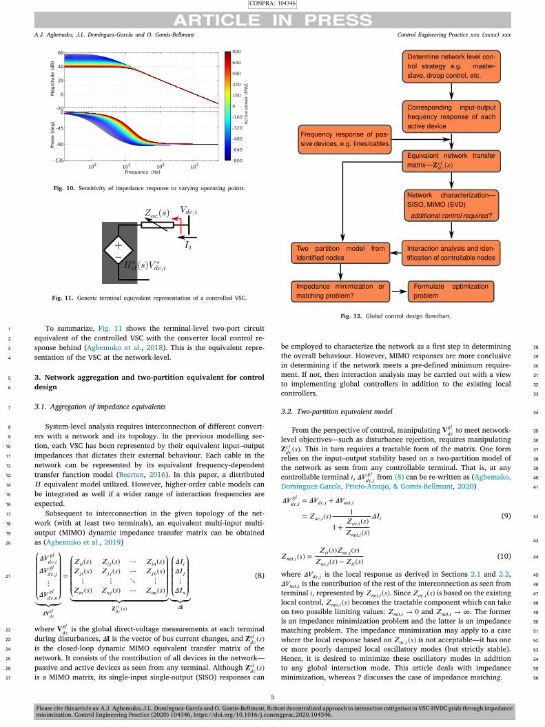
Fig. 11. Generic terminal equivalent representation of a controlled VSC.
To summarize, Fig. 11 shows the terminal-level two-port circuit1
equivalent of the controlled VSC with the converter local control re-2
sponse behind (Agbemuko et al., 2018). This is the equivalent repre-3
sentation of the VSC at the network-level.4
3. Network aggregation and two-partition equivalent for control5
design6
3.1. Aggregation of impedance equivalents7
System-level analysis requires interconnection of different convert-8
ers with a network and its topology. In the previous modelling sec-9
tion, each VSC has been represented by their equivalent input–output10
impedances that dictates their external behaviour. Each cable in the11
network can be represented by its equivalent frequency-dependent12
transfer function model (Beerten, 2016). In this paper, a distributed13
𝛱 equivalent model utilized. However, higher-order cable models can14
be integrated as well if a wider range of interaction frequencies are15
expected.16
Subsequent to interconnection in the given topology of the net-17
work (with at least two terminals), an equivalent multi-input multi-18
output (MIMO) dynamic impedance transfer matrix can be obtained19
as (Agbemuko et al., 2019)20
⎛
⎜
⎜
⎜
⎜
⎜
⎝
𝛥𝑉 𝑔𝑙𝑑𝑐,𝑖
𝛥𝑉 𝑔𝑙𝑑𝑐,𝑗
⋮
𝛥𝑉 𝑔𝑙𝑑𝑐,𝑛
⎞
⎟
⎟
⎟
⎟
⎟
⎠
⏟⏞⏟⏞⏟𝛥𝐕𝑔𝑙
𝑑𝑐
=
⎛
⎜
⎜
⎜
⎜
⎝
𝑍𝑖𝑖(𝑠) 𝑍𝑖𝑗 (𝑠) ⋯ 𝑍𝑖𝑛(𝑠)𝑍𝑗𝑖(𝑠) 𝑍𝑗𝑗 (𝑠) ⋯ 𝑍𝑗𝑛(𝑠)⋮ ⋮ ⋱ ⋮
𝑍𝑛𝑖(𝑠) 𝑍𝑛𝑗 (𝑠) ⋯ 𝑍𝑛𝑛(𝑠)
⎞
⎟
⎟
⎟
⎟
⎠
⏟⏞⏞⏞⏞⏞⏞⏞⏞⏞⏞⏞⏞⏞⏞⏞⏞⏞⏞⏞⏞⏞⏞⏞⏟⏞⏞⏞⏞⏞⏞⏞⏞⏞⏞⏞⏞⏞⏞⏞⏞⏞⏞⏞⏞⏞⏞⏞⏟𝐙𝑐𝑙𝑑𝑐 (𝑠)
⎛
⎜
⎜
⎜
⎜
⎝
𝛥𝐼𝑖𝛥𝐼𝑗⋮
𝛥𝐼𝑛
⎞
⎟
⎟
⎟
⎟
⎠
⏟⏟⏟𝛥𝐈
(8)21
where 𝐕𝑔𝑙𝑑𝑐 is the global direct-voltage measurements at each terminal22
during disturbances, 𝛥𝐈 is the vector of bus current changes, and 𝐙𝑐𝑙𝑑𝑐 (𝑠)23
is the closed-loop dynamic MIMO equivalent transfer matrix of the24
network. It consists of the contribution of all devices in the network—25
passive and active devices as seen from any terminal. Although 𝐙𝑐𝑙𝑑𝑐 (𝑠)26
is a MIMO matrix, its single-input single-output (SISO) responses can27
Fig. 12. Global control design flowchart.
be employed to characterize the network as a first step in determining 28
the overall behaviour. However, MIMO responses are more conclusive 29
in determining if the network meets a pre-defined minimum require- 30
ment. If not, then interaction analysis may be carried out with a view 31
to implementing global controllers in addition to the existing local 32
controllers. 33
3.2. Two-partition equivalent model 34
From the perspective of control, manipulating 𝐕𝑔𝑙𝑑𝑐 to meet network- 35
level objectives—such as disturbance rejection, requires manipulating 36
𝐙𝑐𝑙𝑑𝑐 (𝑠). This in turn requires a tractable form of the matrix. One form 37
relies on the input–output stability based on a two-partition model of 38
the network as seen from any controllable terminal. That is, at any 39
controllable terminal 𝑖, 𝛥𝑉 𝑔𝑙𝑑𝑐,𝑖 from (8) can be re-written as (Agbemuko, 40
Domínguez-García, Prieto-Araujo, & Gomis-Bellmunt, 2020) 41
𝛥𝑉 𝑔𝑙𝑑𝑐,𝑖 = 𝛥𝑉𝑑𝑐,𝑖 + 𝛥𝑉𝑛𝑒𝑡,𝑖
= 𝑍𝑜𝑐,𝑖(𝑠)1
1 +𝑍𝑜𝑐,𝑖(𝑠)𝑍𝑛𝑒𝑡,𝑖(𝑠)
𝛥𝐼𝑖 (9) 42
43
𝑍𝑛𝑒𝑡,𝑖(𝑠) =𝑍𝑖𝑖(𝑠)𝑍𝑜𝑐,𝑖(𝑠)
𝑍𝑜𝑐,𝑖(𝑠) −𝑍𝑖𝑖(𝑠)(10) 44
where 𝛥𝑉𝑑𝑐,𝑖 is the local response as derived in Sections 2.1 and 2.2, 45
𝛥𝑉𝑛𝑒𝑡,𝑖 is the contribution of the rest of the interconnection as seen from 46
terminal 𝑖, represented by 𝑍𝑛𝑒𝑡,𝑖(𝑠). Since 𝑍𝑜𝑐,𝑖(𝑠) is based on the existing 47
local control, 𝑍𝑛𝑒𝑡,𝑖(𝑠) becomes the tractable component which can take 48
on two possible limiting values: 𝑍𝑛𝑒𝑡,𝑖 → 0 and 𝑍𝑛𝑒𝑡,𝑖 → ∞. The former 49
is an impedance minimization problem and the latter is an impedance 50
matching problem. The impedance minimization may apply to a case 51
where the local response based on 𝑍𝑜𝑐,𝑖(𝑠) is not acceptable—it has one 52
or more poorly damped local oscillatory modes (but strictly stable). 53
Hence, it is desired to minimize these oscillatory modes in addition 54
to any global interaction mode. This article deals with impedance 55
minimization, whereas ? discusses the case of impedance matching. 56
5

CONPRA: 104346
Please cite this article as: A.J. Agbemuko, J.L. Domínguez-García and O. Gomis-Bellmunt, Robust decentralized approach to interaction mitigation in VSC-HVDC grids through impedanceminimization. Control Engineering Practice (2020) 104346, https://doi.org/10.1016/j.conengprac.2020.104346.
A.J. Agbemuko, J.L. Domínguez-García and O. Gomis-Bellmunt Control Engineering Practice xxx (xxxx) xxx
Fig. 13. Three terminal VSC-HVDC grid.
Broadly speaking, in both cases the stability margin as seen from1
each terminal is being manipulated. The generalized steps for analysis2
and design of global controllers (if required) are depicted in Fig. 12. The3
optimization formulation is discussed in more detail in later sections.4
4. Application example: Network characterization and interaction5
analysis6
This section presents the first step in determining if additional7
control action is required. For a three-terminal master–slave controlled8
HVDC grid shown in Fig. 13, the characterization, and interaction9
analysis are presented given the local impedance responses derived in10
Section 2—direct-voltage and active power. Data for the HVDC grid is11
presented in Table 1. The HVDC interconnects two AC grid with an12
isolated power system—such as a wind farm, with VSC-1 being the13
direct-voltage controlling terminal and, VSC-2 and 3 in active power14
control modes.15
Given the network-level control strategy and the corresponding16
input–output frequency response of all subsystems, the next step is to17
obtain the network transfer matrix and characterize the network.18
4.1. Equivalent transfer matrix and SISO network characterization19
For the three terminal network shown in Fig. 13 the equivalent20
transfer matrix can be symbolically written as21
𝐙𝑐𝑙𝑑𝑐 (𝑠) =
⎛
⎜
⎜
⎝
𝑍11(𝑠) 𝑍12(𝑠) 𝑍13(𝑠)𝑍12(𝑠) 𝑍22(𝑠) 𝑍23(𝑠)𝑍13(𝑠) 𝑍23(𝑠) 𝑍33(𝑠)
⎞
⎟
⎟
⎠
. (11)22
Given the nominal power flow, the isolated SISO frequency re-23
sponses of the network transfer matrix are shown in Fig. 14 (elements24
in similar colours are equivalent). The diagonal elements predict the25
behaviour of each subsystem (VSCs) relative to the network for dis-26
turbances close to them; whereas off-diagonal elements indicate the27
transfers from other subsystems—in which case they predict the in-28
teractions between terminals. As shown, there appear to be multiple29
resonant frequencies. There are three dominant interaction frequencies30
at 17 Hz, 41 Hz, and 56 Hz respectively. However, some elements show31
all three frequencies with different magnitudes, and others show only32
two. Hence, the SISO frequency response gives a first impression of33
potential resonances during disturbances. Each element predicts the34
dynamic amplification for isolated disturbances from the corresponding35
terminal or between terminals.36
4.2. MIMO network characterization37
The SISO frequency response of 𝐙𝑐𝑙𝑑𝑐 (𝑠) provides rich information on38
the oscillatory behaviour and resonances as contributed by each VSC.39
Particularly, the SISO frequency response gives the isolated behavioural40
responses even though physical responses are often coupled. That is, a41
disturbance at one VSC elicits a reaction from that VSC and other VSCs42
that could go back and forth; this is a MIMO behaviour. Essentially, the 43
𝐙𝑐𝑙𝑑𝑐 (𝑠) transfer matrix should instead be considered as a MIMO transfer 44
matrix rather than a collection of SISO transfer functions. On the other 45
hand, it is important to determine if oscillatory behaviour does indeed 46
warrant additional control action. In this case, the collective response 47
(rather than isolated SISO responses) with respect to defined network 48
specifications indicates the true characterization of the network con- 49
sidering a MIMO behaviour. Specifications can be defined by imposing 50
limits on the maximum singular value of the transfer matrix. For a 51
maximum allowed voltage deviation of 𝛥𝑉 and expected bus current 52
change of 𝛥𝐼 , a limit can be defined as 53
�̄�(𝐙𝑐𝑙𝑑𝑐 ) ≤ 20 log10
‖𝛥𝑉 ‖2‖𝛥𝐼‖2
dB. (12) 54
For a maximum allowed voltage deviation of 40 kV (equivalent to 10% 55
overvoltage), and bus current change of 500 A (equivalent to 200 MW), 56
the limit of maximum singular value is ≈ 40 dB. Fig. 15 shows the cor- 57
responding MIMO responses based on the singular value decomposition 58
(SVD) of the matrix indicating the principal components of responses 59
considering the potential direction of inputs (in this case currents). It 60
shows that the maximum singular value breached the established limits 61
indicated below the grey area. Hence, additional control is required to 62
keep the system within established limits, which may not be possible 63
with existing local control. Therefore, the area below the grey shading 64
in Fig. 15 establishes the benchmark for potential improvements with 65
external controllers. 66
4.3. Interaction analysis 67
The SVD response plot still does not provide information about how 68
the VSCs are contributing to each frequency if there is indeed any 69
interaction. While the SVD response may identify a resonant frequency 70
as dominant, this may not hold from an interaction contribution per- 71
spective. More so, it is important to isolate the different combinations 72
of terminals contributing to an interaction mode to allow efficient tar- 73
geting. The frequency-dependent relative gain array (RGA) defined for 74
MIMO systems is an extraordinary tool for indication of combinations 75
of interactions in MIMO systems (Bristol, 1966). Let 𝐑(𝑠), evaluated at 76
each frequency denote the corresponding RGA of 𝐙𝑐𝑙𝑑𝑐 (𝑠) such that, 77
𝐑(𝑠) = 𝐙𝑐𝑙𝑑𝑐 (𝑠)⊗
(
𝐙𝑐𝑙𝑑𝑐 (𝑠)
)−𝑇 (13) 78
where ⊗ is the Hadamard product (element-wise multiplication). Since 79
𝐑(𝑠) is frequency-dependent, the general criterion that guarantees a 80
non-interacting system at a specified frequency 𝑠 = 𝑗𝜔 is 81
𝐑(𝑗𝑤) = 𝐈 (14) 82
where 𝐈 is the identity matrix. That is, VSCs are not interacting at 83
a specified frequency if 𝐑(𝑠) is unity. On the other hand, they are 84
interacting at a specified frequency if corresponding elements in 𝐙𝑐𝑙𝑑𝑐 (𝑠) 85
show magnitude peaks (≫ 1). For example, if all elements of 𝐙𝑐𝑙𝑑𝑐 (𝑠) 86
show magnitude peaks at a certain frequency, then all VSCs are in- 87
teracting at that frequency. Additionally, RGA also allows determining 88
how inherent coordination could be applied in design when the number 89
of controllers to be designed is less than the number of VSCs in the 90
network. 91
For the studied example, Fig. 16 shows the frequency-dependent 92
RGA magnitude plot based on the network transfer matrix 𝐙𝑐𝑙𝑑𝑐 (𝑠). The 93
combination of terminals contributing to each interaction frequency is 94
shown in the zoomed response. Several observations can be directly 95
made: Observe the first peak where all distinct elements of the matrix 96
show significant peaks; at this frequency, all VSCs are interacting or 97
otherwise contributing to that frequency at different magnitudes. This 98
is due to the interaction between the direct-voltage control and the total 99
capacitance of the DC grid which was not considered in local control. 100
Nevertheless, observation of the first peak is contrary to the SVD plot in 101
Fig. 15 that suggest the most dominant mode as the resonance at 56 Hz 102
6

CONPRA: 104346
Please cite this article as: A.J. Agbemuko, J.L. Domínguez-García and O. Gomis-Bellmunt, Robust decentralized approach to interaction mitigation in VSC-HVDC grids through impedanceminimization. Control Engineering Practice (2020) 104346, https://doi.org/10.1016/j.conengprac.2020.104346.
A.J. Agbemuko, J.L. Domínguez-García and O. Gomis-Bellmunt Control Engineering Practice xxx (xxxx) xxx
Fig. 14. SISO frequency response of the global disturbance transfer matrix.
Fig. 15. SVD plot of the global closed-loop disturbance response matrix.
(third peak). At the second peak, VSCs 1 and 2 are interacting with VSC-1
3 as indicated by the magnitudes of 13, 23, and 33 elements. Whereas,2
at the slightly higher third peak, only VSC-1 and 2 are interacting3
with a relatively higher magnitude than the previous peak (VSC-3 does4
not seem to participate at all this frequency). Further, at steady-state5
and high frequency, diagonal elements approach 1 and off-diagonal6
elements approach 0—non-interacting system in these spectra. From7
this plot, it can be hypothesized that only two controllers at VSC-1 and8
2 are necessary to decouple the system. It makes no sense to have three9
controllers since for each frequency VSC-3 is contributing, either one10
of VSC-1 and/or VSC-2 are also contributing.11
To verify these frequencies from a detailed nonlinear time-domain12
model, Fig. 17 depicts the time-domain responses of direct-voltages for13
a step change at 2.5 s at VSC-3 and the corresponding fast Fourier trans-14
form (FFT). Firstly, the frequencies of resonances match the identified15
frequencies in Fig. 15 at 17 Hz, 41 Hz, and 56 Hz respectively. Secondly,16
for the change in VSC-3, the first two frequencies are more dominant as17
expected from the interaction analysis since the contribution of VSC-318
to the 56 Hz resonance is low. To further demonstrate the effectiveness19
Fig. 16. Frequency-dependent RGA plot.
of the RGA plot in the detection of interactions, Fig. 18 depicts the 20
time-domain response of direct-voltages for a step-change in power 21
reference at VSC-2, with the corresponding FFT of signals. From the 22
RGA response, for changes at VSC-2, VSC-1 contributes significantly to 23
7

CONPRA: 104346
Please cite this article as: A.J. Agbemuko, J.L. Domínguez-García and O. Gomis-Bellmunt, Robust decentralized approach to interaction mitigation in VSC-HVDC grids through impedanceminimization. Control Engineering Practice (2020) 104346, https://doi.org/10.1016/j.conengprac.2020.104346.
A.J. Agbemuko, J.L. Domínguez-García and O. Gomis-Bellmunt Control Engineering Practice xxx (xxxx) xxx
Fig. 17. Non-linear time-domain simulation of system responses and FFT of signals for step change in power from VSC-3.
Fig. 18. Non-linear time-domain simulation of system responses and FFT of signals for step change in power at VSC-2.
the first and third peaks; this is confirmed by the FFT with relatively1
similar magnitudes to the RGA response. At VSC-2 all three peaks can2
be seen and at VSC-3 only the first and second peaks can be seen since3
it does not contribute to the third peak that only involves VSC-1 and 2.4
5. Application example: Control formulation and design of decen-5
tralized global controllers6
The network analysis in the previous section established the need to7
implement global controllers independent of the existing local control.8
The next step from Fig. 12 is to partition the system into two from each9
controllable terminal according to (9). In this case, an impedance min-10
imization problem is desired due to the presence of a poorly damped11
local oscillatory mode in the direct-voltage controlled VSC. That is, it is12
desired to transfer some local responsibilities to the global controller, in13
addition to mitigating interactions with the rest of the network. Hence,14
it is desired that 𝑍𝑛𝑒𝑡,𝑖 → 0 and according to (10) this is equivalent to15
forcing 𝑍𝑖𝑖(𝑠) → 0 from each terminal since there is no access to local16
control based on 𝑍𝑜𝑐,𝑖(𝑠). Therefore, the goal of global control from the17
network view is to minimize the existing transfer matrix 𝐙𝑐𝑙𝑑𝑐 (𝑠) subject18
to constraints.19
5.1. Objectives of design20
First, the objectives are stated, and a description of how the problem21
fits into the ∞ mixed sensitivity framework follows. It is important to22
remark again that this is a disturbance rejection problem. The following23
objectives are paramount:24
1. Reduce the effect of feedback coupling (interaction) between ter-25
minals and dormant network oscillations not considered during26
the individual design of local controllers.27
2. Synthesized controllers must not interact with local controllers. 28
Particularly, it is ideally desired that synthesized controllers van- 29
ish in steady-state. That is, the controllers are only active during 30
transients and disturbances of pre-defined frequency spectrum 31
identified based on 𝐙𝑐𝑙𝑑𝑐 (𝑠). 32
3. More importantly, the controller must not in any manner inter- 33
act with the inner AC control loop which is often the fastest loop 34
and the bandwidth limit of the VSC. 35
In the following subsections, these objectives are translated into 36
frequency domain requirements. 37
5.2. Mixed sensitivity framework 38
Considering that tracking is not an issue as each local controller 39
ensures this, the problem becomes that of minimizing 𝛥𝐕𝑔𝑙𝑑𝑐 = 𝐙𝑐𝑙
𝑑𝑐 (𝑠)𝛥𝐈 40
due to the interconnection with other VSCs, subject to constraints. 41
Constraints include the maximum allowed control effort to minimize 42
𝛥𝐕𝑔𝑙𝑑𝑐 . Therefore, the overall problem is a mixed-sensitivity problem of 43
disturbance and control input. 44
Fig. 19 describes the problem in the generalized framework of 45
∞ (Skogestad & Postlethwaite, 2007). 𝐙𝑝 = 𝛼𝐼 is a fictitious plant 46
model (𝛼 is determined by iteration and to prevent the synthesis of 47
a large gain controller); in this work, 𝛼 = [1–500]. This ensures that 48
the minimization problem is wholly dominated by 𝐙𝑐𝑙𝑑𝑐 (𝑠). 𝐖𝑝(𝑠) is 49
the output weighting matrix that determines by how much 𝛥𝐕𝑔𝑙𝑑𝑐 is 50
minimized (objective 1), 𝐖𝑢(𝑠) is the control output weighting matrix 51
(objectives 2 and 3), and 𝐊(𝑠) is a diagonal matrix of synthesized 52
controllers (Gahinet & Apkarian, 2011). It must be noted that this is 53
a MIMO problem and all matrices are MIMO matrices with lengths 54
equal to the number of subsystems. The closed-loop expressions of 55
the augmented system can be derived from Fig. 19. Starting with the 56
8

CONPRA: 104346
Please cite this article as: A.J. Agbemuko, J.L. Domínguez-García and O. Gomis-Bellmunt, Robust decentralized approach to interaction mitigation in VSC-HVDC grids through impedanceminimization. Control Engineering Practice (2020) 104346, https://doi.org/10.1016/j.conengprac.2020.104346.
A.J. Agbemuko, J.L. Domínguez-García and O. Gomis-Bellmunt Control Engineering Practice xxx (xxxx) xxx
Fig. 19. Block diagram of plant interconnections.
inner-most structure (dashed red box)1
𝑧1(𝑠) = 𝐖𝑢(𝑠)𝛥𝐈𝑠𝑧2(𝑠) = 𝐖𝑝(𝑠)𝐙𝑐𝑙
𝑑𝑐 (𝑠)𝛥𝐈 +𝐖𝑝(𝑠)𝐙𝑝(𝑠)𝛥𝐈𝑠𝛥𝐕 = 𝐙𝑐𝑙
𝑑𝑐 (𝑠)𝛥𝐈 + 𝐙𝑝(𝑠)𝛥𝐈𝑠.(15)2
The above expressions can be written compactly as3
[
𝐳𝛥𝐕
]
=[
𝑃11 𝑃12𝑃21 𝑃22
]
⏟⏞⏞⏞⏞⏟⏞⏞⏞⏞⏟𝐏
[
𝛥𝐈𝛥𝐈𝑠
]
, 𝐳 =[
𝑧1𝑧2
]
(16)4
where 𝐏 is the augmented plant with target weights 𝐖𝑝 and 𝐖𝑢, 𝑧1 and5
𝑧2 are the outputs to be minimized, 𝛥𝐕 is the input to controller, 𝛥𝐈 is6
the disturbance, and 𝛥𝐈𝑠 as the control input. The (s) term for transfer7
functions is henceforth neglected. The 𝐏 matrix can be expanded as8
𝐏 =
⎡
⎢
⎢
⎢
⎣
0𝐖𝑝𝐙𝑐𝑙
𝑑𝑐
𝐖𝑢𝐖𝑝𝐙𝑝
𝐙𝑐𝑙𝑑𝑐 𝐙𝑝
⎤
⎥
⎥
⎥
⎦
. (17)9
After interconnection with the controller(s) to be synthesized, then10
the controller outputs 𝛥𝐈𝑠 = −𝐊𝛥𝐕 can be eliminated to obtain11
𝑧1 = −𝐖𝑢𝐊𝛥𝐕𝑧2 = 𝐖𝑝𝐙𝑐𝑙
𝑑𝑐𝛥𝐈 −𝐖𝑝𝐙𝑝𝐊𝛥𝐕𝛥𝐕 = 𝐙𝑐𝑙
𝑑𝑐𝛥𝐈 − 𝐙𝑝𝐊𝛥𝐕
⟹ 𝛥𝐕 = 𝐈𝐈 + 𝐙𝑝𝐊⏟⏞⏟⏞⏟
𝐒
𝐙𝑐𝑙𝑑𝑐
⏟⏞⏞⏞⏞⏞⏟⏞⏞⏞⏞⏞⏟𝐙𝑐𝑙𝑑𝑐,𝑛𝑒𝑤
𝛥𝐈 (18)12
where 𝐒 is the sensitivity transfer matrix of the synthesized controllers,13
𝐙𝑐𝑙𝑑𝑐,𝑛𝑒𝑤 is the modified transfer matrix of the network, and 𝛥𝐕 can be14
eliminated from 𝑧1 and 𝑧2 to obtain15
𝑧1 = −𝐖𝑢𝐊𝐒𝐙𝑐𝑙𝑑𝑐𝛥𝐈
𝑧2 = 𝐖𝑝𝐒𝐙𝑐𝑙𝑑𝑐𝛥𝐈.
(19)16
The above expressions can be written compactly as17
𝐳 = 𝐍(𝐊)𝛥𝐈. (20)18
The optimization problem becomes that of minimizing the ∞ norm of19
the closed loop transfer function 𝐍 subject to a given stable controller20
such that21
min𝐾
‖𝐍(𝐾)‖∞ ≤ 𝛾, 𝐍(𝐾) =[
𝐖𝑢𝐊𝐒𝐆𝑑𝐖𝑝𝐒𝐆𝑑
]
(21)22
where 𝛾 is the desired closed-loop gain.23
5.3. Design preliminaries24
5.3.1. Scaling25
A key priority for a successful implementation is proper scaling to26
prevent potential skewing of the mixed-sensitivity problem. Scaling is27
Table 3Scaling factors.
Parameter Value Comments
𝛥𝑉𝑚𝑎𝑥 40 kV Allowed voltage deviation𝛥𝐼𝑠,𝑚𝑎𝑥 0.8 kA Allowed control input𝛥𝐼𝑚𝑎𝑥 0.5 kA Expected disturbance
Table 4Design weights.
𝑊𝑝 𝑊𝑢
VSC-1 0.5 𝑠+2𝜔𝑝1
𝑠+𝜔𝑝1500
0.75 𝑠+2𝑠+𝜔𝑢1
VSC-2 0.45 𝑠+2𝜔𝑝2
𝑠+𝜔𝑝2450
0.65 𝑠𝑠+𝜔𝑢2
VSC-3 0.45 𝑠+2𝜔𝑝3
𝑠+𝜔𝑝3450
0.65 𝑠𝑠+𝜔𝑢3
done according to the recommendations in Skogestad and Postlethwaite 28
(2007) by determination of maximum expected change in inputs, max- 29
imum allowed control input to correct output error, and maximum 30
allowed output for each subsystem. Scalings at each subsystem can 31
emphasize the priority or role of each subsystem. For example, a 32
maximum of 20 kV may be allowed at one subsystem, while only 10 kV 33
may be allowed at another subsystem. However, for simplicity in this 34
paper, the scaling is similar at all subsystems as given in Table 3. The 35
fictitious plant model 𝐙𝑝 and transfer matrix 𝐙𝑐𝑙𝑑𝑐 are scaled according 36
to 37
𝐙𝑠𝑝 = 𝛥𝐕−1
𝑚𝑎𝑥𝐙𝑝𝛥𝐈𝑠,𝑚𝑎𝑥𝐙𝑐𝑙,𝑠𝑑𝑐 = 𝛥𝐕−1
𝑚𝑎𝑥𝐙𝑐𝑙𝑑𝑐𝛥𝐈𝑚𝑎𝑥
(22) 38
where 𝐈𝑠,𝑚𝑎𝑥 is the maximum allowed control input to minimize output, 39
and 𝐈𝑚𝑎𝑥 is the maximum expected disturbance. 40
5.3.2. Model reduction 41
To keep the problem as tractable as possible by preventing nu- 42
merical artefacts, a low order equivalent model is sought for the key 43
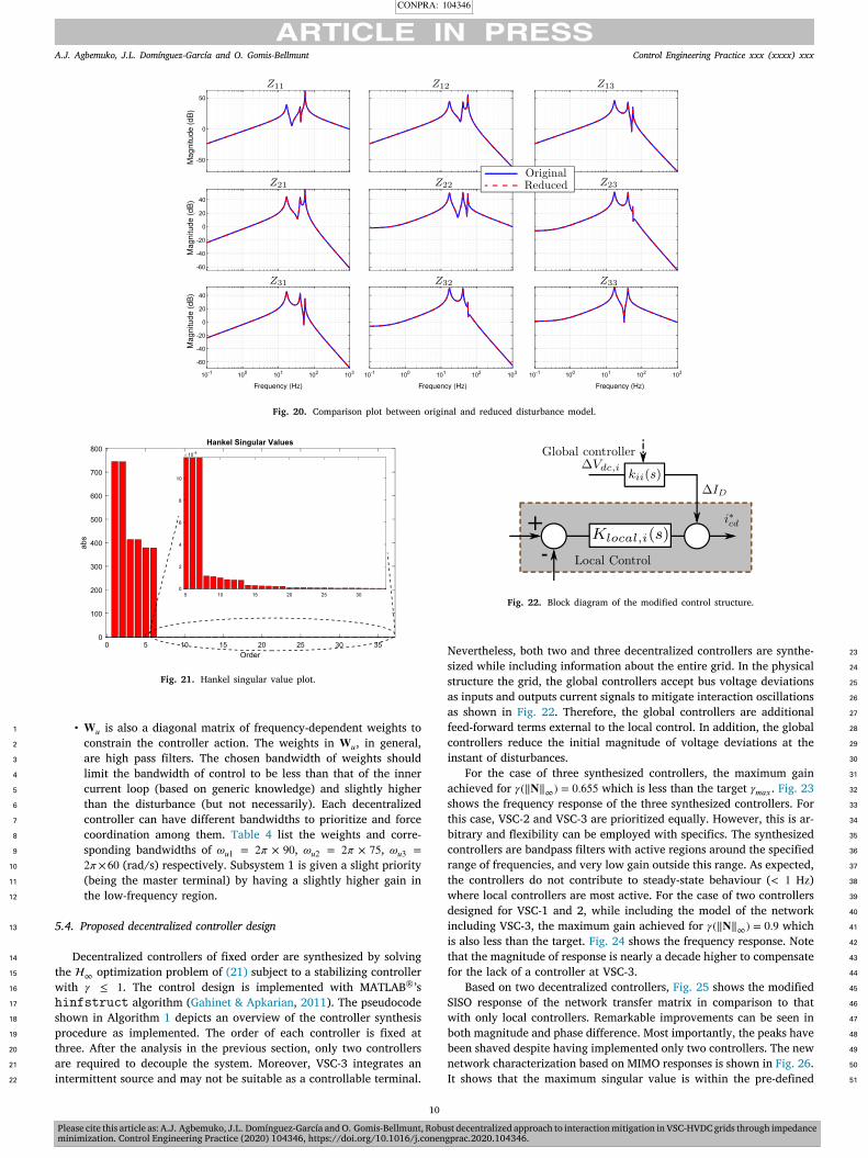
transfer matrix 𝐙𝑐𝑙𝑑𝑐 . The Hankel balanced reduction method is applied 44
for reduction. In this paper, the total order of 𝐙𝑐𝑙𝑑𝑐 is 35 before reduction 45
and 7 after reduction. Fig. 20 shows the comparison of the original 46
model and the equivalent reduced model, whereas, Fig. 21 depicts the 47
Hankel’s singular value plot showing the dominant states. 48
5.3.3. Order and structure of controller 49
A key priority is to obtain adoptable low-order fixed structure 50
controllers. It is well known that the order of synthesized controller 51
with standard ∞ is quite high while assuming a centralized structure. 52
Several methods to reduce the order have been suggested in literature. 53
However, in this paper, decentralized controllers, with a maximum 54
order of three was preferred for transparency and to eliminate any 55
communication requirements of the centralized structure. The real- 56
ized third-order structure is reducible to two without any change in 57
performance if desired. 58
5.3.4. Weight selection and justification 59
The choice of weights 𝐖𝑝 and 𝐖𝑢 are influenced by the actual 60
frequency domain responses, and iteration may be required to obtain 61
the best weights. 62
• 𝐖𝑝 is a diagonal matrix of frequency-dependent weights that 63
determine the target sensitivity of control. For the impedance 64
minimization problem, a simple choice of a high gain low-pass 65
filter with a bandwidth equal to the frequency of disturbances 66
to be rejected can be selected. Bandwidth and magnitude of 67
weights can be chosen to reflect the priority of each subsystem or 68
coordination as obtained from the RGA plot. The chosen weights 69
for the base case can be found in Table 4 with a bandwidth of 70
𝜔𝑝1 = 𝜔𝑝2 = 𝜔𝑝3 = 2𝜋×65 (rad/s) respectively for each subsystem. 71
9
CONPRA: 104346
Please cite this article as: A.J. Agbemuko, J.L. Domínguez-García and O. Gomis-Bellmunt, Robust decentralized approach to interaction mitigation in VSC-HVDC grids through impedanceminimization. Control Engineering Practice (2020) 104346, https://doi.org/10.1016/j.conengprac.2020.104346.
A.J. Agbemuko, J.L. Domínguez-García and O. Gomis-Bellmunt Control Engineering Practice xxx (xxxx) xxx
Fig. 20. Comparison plot between original and reduced disturbance model.
Fig. 21. Hankel singular value plot.
• 𝐖𝑢 is also a diagonal matrix of frequency-dependent weights to1
constrain the controller action. The weights in 𝐖𝑢, in general,2
are high pass filters. The chosen bandwidth of weights should3
limit the bandwidth of control to be less than that of the inner4
current loop (based on generic knowledge) and slightly higher5
than the disturbance (but not necessarily). Each decentralized6
controller can have different bandwidths to prioritize and force7
coordination among them. Table 4 list the weights and corre-8
sponding bandwidths of 𝜔𝑢1 = 2𝜋 × 90, 𝜔𝑢2 = 2𝜋 × 75, 𝜔𝑢3 =9
2𝜋×60 (rad/s) respectively. Subsystem 1 is given a slight priority10
(being the master terminal) by having a slightly higher gain in11
the low-frequency region.12
5.4. Proposed decentralized controller design13
Decentralized controllers of fixed order are synthesized by solving14
the ∞ optimization problem of (21) subject to a stabilizing controller15
with 𝛾 ≤ 1. The control design is implemented with MATLAB®’s16
hinfstruct algorithm (Gahinet & Apkarian, 2011). The pseudocode17
shown in Algorithm 1 depicts an overview of the controller synthesis18
procedure as implemented. The order of each controller is fixed at19
three. After the analysis in the previous section, only two controllers20
are required to decouple the system. Moreover, VSC-3 integrates an21
intermittent source and may not be suitable as a controllable terminal.22
Fig. 22. Block diagram of the modified control structure.
Nevertheless, both two and three decentralized controllers are synthe- 23
sized while including information about the entire grid. In the physical 24
structure the grid, the global controllers accept bus voltage deviations 25
as inputs and outputs current signals to mitigate interaction oscillations 26
as shown in Fig. 22. Therefore, the global controllers are additional 27
feed-forward terms external to the local control. In addition, the global 28
controllers reduce the initial magnitude of voltage deviations at the 29
instant of disturbances. 30
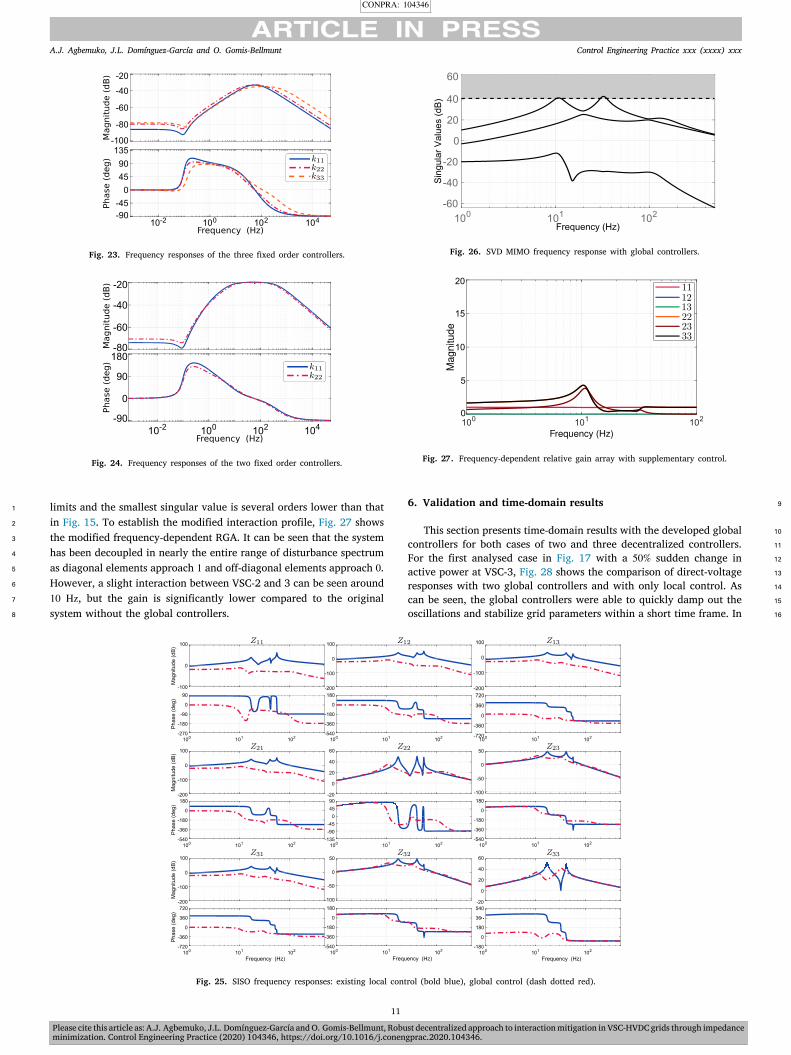
For the case of three synthesized controllers, the maximum gain 31
achieved for 𝛾(‖𝐍‖∞) = 0.655 which is less than the target 𝛾𝑚𝑎𝑥. Fig. 23 32
shows the frequency response of the three synthesized controllers. For 33
this case, VSC-2 and VSC-3 are prioritized equally. However, this is ar- 34
bitrary and flexibility can be employed with specifics. The synthesized 35
controllers are bandpass filters with active regions around the specified 36
range of frequencies, and very low gain outside this range. As expected, 37
the controllers do not contribute to steady-state behaviour (< 1 Hz) 38
where local controllers are most active. For the case of two controllers 39
designed for VSC-1 and 2, while including the model of the network 40
including VSC-3, the maximum gain achieved for 𝛾(‖𝐍‖∞) = 0.9 which 41
is also less than the target. Fig. 24 shows the frequency response. Note 42
that the magnitude of response is nearly a decade higher to compensate 43
for the lack of a controller at VSC-3. 44
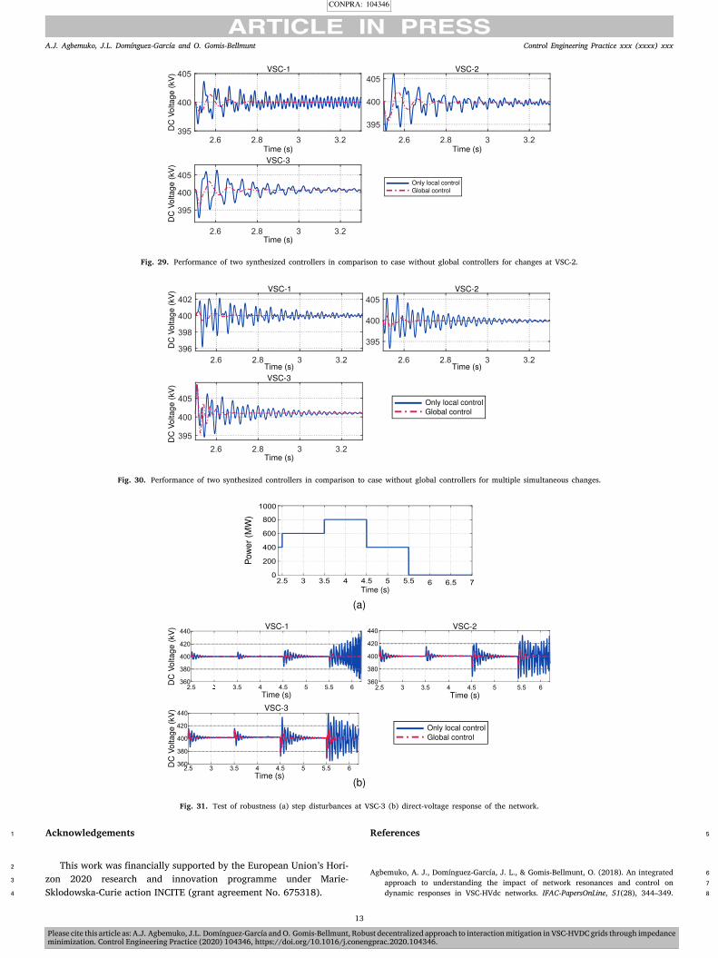
Based on two decentralized controllers, Fig. 25 shows the modified 45
SISO response of the network transfer matrix in comparison to that 46
with only local controllers. Remarkable improvements can be seen in 47
both magnitude and phase difference. Most importantly, the peaks have 48
been shaved despite having implemented only two controllers. The new 49
network characterization based on MIMO responses is shown in Fig. 26. 50
It shows that the maximum singular value is within the pre-defined 51
10
CONPRA: 104346
Please cite this article as: A.J. Agbemuko, J.L. Domínguez-García and O. Gomis-Bellmunt, Robust decentralized approach to interaction mitigation in VSC-HVDC grids through impedanceminimization. Control Engineering Practice (2020) 104346, https://doi.org/10.1016/j.conengprac.2020.104346.
A.J. Agbemuko, J.L. Domínguez-García and O. Gomis-Bellmunt Control Engineering Practice xxx (xxxx) xxx
Fig. 23. Frequency responses of the three fixed order controllers.
Fig. 24. Frequency responses of the two fixed order controllers.
limits and the smallest singular value is several orders lower than that1
in Fig. 15. To establish the modified interaction profile, Fig. 27 shows2
the modified frequency-dependent RGA. It can be seen that the system3
has been decoupled in nearly the entire range of disturbance spectrum4
as diagonal elements approach 1 and off-diagonal elements approach 0.5
However, a slight interaction between VSC-2 and 3 can be seen around6
10 Hz, but the gain is significantly lower compared to the original7
system without the global controllers.8
Fig. 26. SVD MIMO frequency response with global controllers.
Fig. 27. Frequency-dependent relative gain array with supplementary control.
6. Validation and time-domain results 9
This section presents time-domain results with the developed global 10
controllers for both cases of two and three decentralized controllers. 11
For the first analysed case in Fig. 17 with a 50% sudden change in 12
active power at VSC-3, Fig. 28 shows the comparison of direct-voltage 13
responses with two global controllers and with only local control. As 14
can be seen, the global controllers were able to quickly damp out the 15
oscillations and stabilize grid parameters within a short time frame. In 16
Fig. 25. SISO frequency responses: existing local control (bold blue), global control (dash dotted red).
11

CONPRA: 104346
Please cite this article as: A.J. Agbemuko, J.L. Domínguez-García and O. Gomis-Bellmunt, Robust decentralized approach to interaction mitigation in VSC-HVDC grids through impedanceminimization. Control Engineering Practice (2020) 104346, https://doi.org/10.1016/j.conengprac.2020.104346.
A.J. Agbemuko, J.L. Domínguez-García and O. Gomis-Bellmunt Control Engineering Practice xxx (xxxx) xxx
Fig. 28. Performance of two synthesized controllers in comparison to case without global controllers for changes at VSC-3.
Algorithm 1 Decentralized global controller synthesis1: Definitions and model preliminaries:
𝛥𝐕𝑚𝑎𝑥 = diag(𝛥𝑉𝑚𝑎𝑥,𝑖,⋯ , 𝛥𝑉𝑚𝑎𝑥,𝑛);𝛥𝐈𝑠,𝑚𝑎𝑥 = diag(𝛥𝐼𝑠𝑚𝑎𝑥,𝑖,⋯ , 𝛥𝐼𝑠𝑚𝑎𝑥,𝑛);𝛥𝐈𝑚𝑎𝑥 = diag(𝛥𝐼𝑚𝑎𝑥,𝑖,⋯ , 𝛥𝐼𝑚𝑎𝑥,𝑛)
2: Process/Disturbance Models:𝑧𝑝𝑖𝑖 = 𝛼𝑖𝑖 ∗ tf(1, 1); ⋯ 𝑧𝑝𝑛𝑛 = 𝛼𝑛𝑛 ∗ tf(1, 1);𝐙𝑝 = blckdiag(𝑧𝑝𝑖𝑖,⋯ 𝑧𝑝𝑛𝑛); 𝐙𝑐𝑙
𝑑𝑐 = tf(⋯);3: Model reduction:
[𝐙𝑐𝑙𝑑𝑐,𝑟𝑒𝑑 ] = reduce(𝐙𝑐𝑙
𝑑𝑐 ,order);4: Scaling:
𝐙𝑠𝑝 = 𝛥𝐕−1𝐙𝑝𝛥𝐈𝑠;
𝐙𝑐𝑙,𝑠𝑑𝑐 = 𝛥𝐕−1𝐙𝑐𝑙
𝑑𝑐,𝑟𝑒𝑑𝛥𝐈; % goto 1 for scaling parameters5: Weighting Matrices:
𝑤𝑢𝑖 = tf(⋯); ⋯ 𝑤𝑢𝑛 = tf(⋯);𝐖𝑢 = blkdiag(𝑤𝑢𝑖,⋯𝑤𝑢𝑛);𝑤𝑝𝑖 = tf(⋯); ⋯ 𝑤𝑝𝑛 = tf(⋯);𝐖𝑝 = blkdiag(𝑤𝑝𝑖,⋯𝑤𝑝𝑛);
6: Controller order specification:𝑘𝑖𝑖 = tf([𝑏𝑛−1, 𝑏𝑛−2,⋯ 𝑏0], [𝑎𝑛, 𝑎𝑛−1,⋯ 𝑎0]); % 𝑛 is the order ofcontroller, 𝑎 and 𝑏 are free parameters𝐊 = blkdiag(𝑘𝑖𝑖,⋯ 𝑘𝑛𝑛);
7: 𝐏 assembly and interconnection:𝐙𝑐𝑙𝑑𝑐,𝑟𝑒𝑑 .u = ‘𝑑𝐼’; 𝐙𝑐𝑙
𝑑𝑐,𝑟𝑒𝑑 .y = ‘𝑤’;𝐖𝑢.u = ‘𝑑𝐼𝑠’; 𝐖𝑢.y = ‘𝑧1’;𝐖𝑝.u = ‘𝑑𝑉 ’; 𝐖𝑝.y = ‘𝑧2’;𝐊.u = ‘𝑑𝑉 ’; 𝐊.y = ‘𝑑𝐼𝑠’;𝐙𝑠𝑝.u = ‘𝑑𝐼𝑠’; 𝐙𝑠
𝑝.y = ‘𝑜𝑢𝑡𝑝𝑢𝑡’;sumoutput = sumblk(‘𝑑𝑉 = 𝑤 + 𝑜𝑢𝑡𝑝𝑢𝑡’, 𝑛); % 𝑛 is thedimension of the MIMO system
8: 𝐍 assembly:connect(⋯); % make the interconnection
9: Controller synthesis:[𝐊, 𝛾,info] = hinfstruct(𝐍);
10: if 𝛾 > 𝛾𝑚𝑎𝑥 then11: goto 5 % adapt weighting matrices12: end if13: Transfer function of synthesized controllers:
showTunable(𝐊);
the second case of Fig. 18 for a similar step-change in active power1
at VSC-2, Fig. 29 shows the grid direct-voltage responses. It can be2
seen that despite the higher distortion across several frequencies as in3
case with only local control, the global controllers are able to quickly4
mitigate the oscillatory behaviour. The only oscillatory behaviour is 5
that due to the interaction between VSC-2 and VSC-3 at 10.3 Hz as 6
shown in the RGA in Fig. 27. However, this damps out within 200 ms. 7
In a severe case of sudden simultaneous changes at both VSC-2 and 8
3 (50% and 30% steps changes respectively), Fig. 30 shows a comparison 9
between only local control and two global controllers. Despite a lack of 10
global controller at VSC-3 at a cost of a slightly degraded response, sim- 11
ilar performance as in previous cases demonstrate the improvements 12
from the global control. 13
To further demonstrate the robustness of synthesized controllers 14
(two decentralized) in a more stringent scenario, Fig. 31 depicts the 15
direct-voltage responses across varying operating points. It can be 16
seen that in the case with only local control, the system lost after 17
a sudden disconnection of VSC-3 initially supplying power into the 18
network. However, with the two synthesized global controllers, the 19
network maintained its robust stability facilitated by the controllers, 20
while mitigating detrimental oscillations. As expected for VSC-3, the 21
response is slightly degraded. Nevertheless, the performance is quite 22
better and acceptable than with only local control. 23
7. Conclusion 24
In summary, this paper proposed the formulation and design of 25
decentralized global controllers to decouple converters in a VSC-HVDC 26
grids through network impedance shaping. First, it was determined if 27
the characterization of the network through MIMO treatment meets 28
pre-defined minimum requirements. In the case the network does not 29
meet this requirement, then RGA can be applied to identify cross- 30
interactions between VSCs and the mechanism of these interactions. 31
Then, robust controllers are synthesized by fitting the problem into 32
an ∞ convex optimization framework. Importantly, these controllers 33
can be designed and implemented using only measurable input-out 34
impedances of VSCs and the availability of an additional control chan- 35
nel. Overall, it can be seen that despite the order of the system, the 36
designed low order controllers were able to robustly decouple the 37
system as demonstrated. Therefore, the method presented offer network 38
operators a flexible and scalable approach in securely interconnecting 39
independently designed converters. 40
Declaration of competing interest 41
The authors declare that they have no known competing finan- 42
cial interests or personal relationships that could have appeared to 43
influence the work reported in this paper. 44
12
CONPRA: 104346
Please cite this article as: A.J. Agbemuko, J.L. Domínguez-García and O. Gomis-Bellmunt, Robust decentralized approach to interaction mitigation in VSC-HVDC grids through impedanceminimization. Control Engineering Practice (2020) 104346, https://doi.org/10.1016/j.conengprac.2020.104346.
A.J. Agbemuko, J.L. Domínguez-García and O. Gomis-Bellmunt Control Engineering Practice xxx (xxxx) xxx
Fig. 29. Performance of two synthesized controllers in comparison to case without global controllers for changes at VSC-2.
Fig. 30. Performance of two synthesized controllers in comparison to case without global controllers for multiple simultaneous changes.
Fig. 31. Test of robustness (a) step disturbances at VSC-3 (b) direct-voltage response of the network.
Acknowledgements1
This work was financially supported by the European Union’s Hori-2
zon 2020 research and innovation programme under Marie-3
Sklodowska-Curie action INCITE (grant agreement No. 675318).4
References 5
Agbemuko, A. J., Domínguez-García, J. L., & Gomis-Bellmunt, O. (2018). An integrated 6
approach to understanding the impact of network resonances and control on 7
dynamic responses in VSC-HVdc networks. IFAC-PapersOnLine, 51(28), 344–349. 8
13

CONPRA: 104346
Please cite this article as: A.J. Agbemuko, J.L. Domínguez-García and O. Gomis-Bellmunt, Robust decentralized approach to interaction mitigation in VSC-HVDC grids through impedanceminimization. Control Engineering Practice (2020) 104346, https://doi.org/10.1016/j.conengprac.2020.104346.
A.J. Agbemuko, J.L. Domínguez-García and O. Gomis-Bellmunt Control Engineering Practice xxx (xxxx) xxx
http://dx.doi.org/10.1016/j.ifacol.2018.11.726, 10th IFAC Symposium on Control1
of Power and Energy Systems CPES 2018.2
Agbemuko, A. J., Domínguez-García, J. L., Prieto-Araujo, E., & Gomis-Bellmunt, O.3
(2019). Dynamic modelling and interaction analysis of multi-terminal VSC-HVDC4
grids through an impedance-based approach. International Journal of Electrical Power5
& Energy Systems, 113, 874–887. http://dx.doi.org/10.1016/j.ijepes.2019.06.029.6
Agbemuko, A. J., Domínguez-García, J. L., Prieto-Araujo, E., & Gomis-Bellmunt, O.7
(2020). Advanced impedance-based control design for decoupling multi-vendor8
converter hvdc grids. IEEE Transactions on Power Delivery, [ISSN: 1937-4208] 1–1.9
http://dx.doi.org/10.1109/TPWRD.2020.2968761.10
Amin, M., & Molinas, M. (2019). A gray-box method for stability and controller11
parameter estimation in HVDC-connected wind farms based on nonparametric12
impedance. IEEE Transactions on Industrial Electronics, 66(3), 1872–1882. http:13
//dx.doi.org/10.1109/TIE.2018.2840516.14
Amin, M., Rygg, A., & Molinas, M. (2016). Impedance-based and eigenvalue based15
stability assessment compared in VSC-HVDC system. In 2016 IEEE energy conversion16
congress and exposition (ECCE) (pp. 1–8). http://dx.doi.org/10.1109/ECCE.2016.17
7855185.18
Beerten, J. (2016). Frequency-dependent cable modelling for small-signal stability19
analysis of vsc-hvdc systems. IET Generation, Transmission & Distribution, 10(11),20
1370–1381.21
Beerten, J., D’Arco, S., & Suul, J. A. (2016). Identification and small-signal analysis22
of interaction modes in VSC MTDC systems. IEEE Transactions on Power Delivery,23
31(2), 888–897. http://dx.doi.org/10.1109/TPWRD.2015.2467965.24
Bose, B. K. (2013). Global energy scenario and impact of power electronics in 21st25
century. IEEE Transactions on Industrial Electronics, 60(7), 2638–2651. http://dx.26
doi.org/10.1109/TIE.2012.2203771.27
Bristol, E. (1966). On a new measure of interaction for multivariable process control.28
IEEE Transactions on Automatic Control, 11(1), 133–134. http://dx.doi.org/10.1109/29
TAC.1966.1098266.30
Céspedes, M., & Sun, J. (2012). Impedance shaping of three-phase grid-parallel voltage-31
source converters. In 2012 twenty-seventh annual IEEE applied power electronics32
conference and exposition (APEC) (pp. 754–760). http://dx.doi.org/10.1109/APEC.33
2012.6165904.34
Cobreces, S., Bueno, E. J., Rodriguez, F. J., Pizarro, D., & Huerta, F. (2010).35
Robust loop-shaping 𝐻∞ control of LCL-connected grid converters. In 2010 IEEE36
international symposium on industrial electronics (pp. 3011–3017). http://dx.doi.org/37
10.1109/ISIE.2010.5637614.38
Cóbreces, S., Wang, X., Pérez, J., Griñó, R., & Blaabjerg, F. (2018). Robust admittance39
shaping approach to grid current harmonic attenuation and resonance damping.40
IEEE Transactions on Industry Applications, 54(5), 5039–5053. http://dx.doi.org/10.41
1109/TIA.2018.2845358.42
Cole, S., Beerten, J., & Belmans, R. (2010). Generalized dynamic VSC MTDC model43
for power system stability studies. IEEE Transactions on Power Systems, 25(3),44
1655–1662. http://dx.doi.org/10.1109/TPWRS.2010.2040846.45
Flourentzou, N., Agelidis, V. G., & Demetriades, G. D. (2009). Vsc-based hvdc power46
transmission systems: An overview. IEEE Transactions on Power Electronics, 24(3),47
592–602. http://dx.doi.org/10.1109/TPEL.2008.2008441.48
Freijedo, F. D., Rodriguez-Diaz, E., Golsorkhi, M. S., Vasquez, J. C., & Guerrero, J. M.49
(2017). A root-locus design methodology derived from the impedance/admittance50
stability formulation and its application for lcl grid-connected converters in wind51
turbines. IEEE Transactions on Power Electronics, 32(10), 8218–8228. http://dx.doi.52
org/10.1109/TPEL.2016.2645862.53
Gabe, I. J., Montagner, V. F., & Pinheiro, H. (2009). Design and implementation of a54
robust current controller for VSI connected to the grid through an LCL filter. IEEE55
Transactions on Power Electronics, 24(6), 1444–1452. http://dx.doi.org/10.1109/56
TPEL.2009.2016097.57
Gahinet, P., & Apkarian, P. (2011). Decentralized and fixed-structure H∞ control in58
matlab. In 2011 50th IEEE conference on decision and control and european control59
conference (pp. 8205–8210). http://dx.doi.org/10.1109/CDC.2011.6160298.60
Haileselassie, T., & Uhlen, K. (2013). Power system security in a meshed North Sea61
HVDC grid. Proceedings of the IEEE, 101(4), 978–990. http://dx.doi.org/10.1109/62
JPROC.2013.2241375.63
Harnefors, L., Bongiorno, M., & Lundberg, S. (2007). Input-admittance calculation and64
shaping for controlled voltage-source converters. IEEE Transactions on Industrial65
Electronics, 54(6), 3323–3334. http://dx.doi.org/10.1109/TIE.2007.904022.66
Harnefors, L., Yepes, A. G., Vidal, A., & Doval-Gandoy, J. (2015). Passivity-based 67
controller design of grid-connected vscs for prevention of electrical resonance 68
instability. IEEE Transactions on Industrial Electronics, 62(2), 702–710. http://dx. 69
doi.org/10.1109/TIE.2014.2336632. 70
He, J., & Li, Y. W. (2012). Generalized closed-loop control schemes with embedded 71
virtual impedances for voltage source converters with LC or LCL filters. IEEE 72
Transactions on Power Electronics, 27(4), 1850–1861. http://dx.doi.org/10.1109/ 73
TPEL.2011.2168427. 74
Hertem, D. V., & Ghandhari, M. (2010). Multi-terminal VSC HVDC for the european 75
supergrid: Obstacles. Renewable & Sustainable Energy Reviews, 14(9), 3156–3163. 76
http://dx.doi.org/10.1016/j.rser.2010.07.068, URL http://www.sciencedirect.com/ 77
science/article/pii/S1364032110002480. 78
Kalcon, G. O., Adam, G. P., Anaya-Lara, O., Lo, S., & Uhlen, K. (2012). Small- 79
signal stability analysis of multi-terminal VSC-based DC transmission systems. 80
IEEE Transactions on Power Systems, 27(4), 1818–1830. http://dx.doi.org/10.1109/ 81
TPWRS.2012.2190531. 82
Kammer, C., D’Arco, S., Endegnanew, A. G., & Karimi, A. (2019). Convex optimization- 83
based control design for parallel grid-connected inverters. IEEE Transactions 84
on Power Electronics, 34(7), 6048–6061. http://dx.doi.org/10.1109/TPEL.2018. 85
2881196. 86
Pea-Alzola, R., Liserre, M., Blaabjerg, F., Ordonez, M., & Yang, Y. (2014). Lcl-filter 87
design for robust active damping in grid-connected converters. IEEE Transactions 88
on Industrial Informatics, 10(4), 2192–2203. http://dx.doi.org/10.1109/TII.2014. 89
2361604. 90
Pérez, J., Cobreces, S., Gri, R., & Sánchez, F. J. R. (2017). 𝐻∞ current controller for 91
input admittance shaping of VSC-based grid applications. IEEE Transactions on Power 92
Electronics, 32(4), 3180–3191. http://dx.doi.org/10.1109/TPEL.2016.2574560. 93
Pinares, G., Tjernberg, L. B., Tuan, L. A., Breitholtz, C., & Edris, A. A. (2013). 94
On the analysis of the dc dynamics of multi-terminal VSC-HVDC systems using 95
small signal modeling. In PowerTech (POWERTECH), 2013 IEEE grenoble (pp. 1–6). 96
http://dx.doi.org/10.1109/PTC.2013.6652303. 97
Prieto-Araujo, E., Egea-Alvarez, A., Fekriasl, S., & Gomis-Bellmunt, O. (2016). DC 98
voltage droop control design for multiterminal HVDC systems considering AC 99
and DC grid dynamics. IEEE Transactions on Power Delivery, 31(2), 575–585. http: 100
//dx.doi.org/10.1109/TPWRD.2015.2451531. 101
Qoria, T., Prevost, T., Denis, G., Gruson, F., Colas, F., & Guillaud, X. (2019). Power 102
converters classification and characterization in power transmission systems. EPE’19 103
ICCE EUROPE. 104
Rault, P. (2019). Implementation of a dedicated control to limit adverse interaction in 105
multi-vendor HVDC systems. IET Conference Proceedings, (1), 7(6 pp.). 106
Schettler, F., Huang, H., & Christl, N. (2000). HVDC transmission systems using voltage 107
sourced converters design and applications. In 2000 power engineering society summer 108
meeting (Cat. No.00CH37134), Vol. 2 (pp. 715–720). http://dx.doi.org/10.1109/ 109
PESS.2000.867439. 110
Skogestad, S., & Postlethwaite, I. (2007). Multivariable feedback control: analysis and 111
design, Vol. 2. Wiley New York. 112
Staudt, V., Steimel, A., Kohlmann, M., Jäger, M. K., Heising, C., Meyer, D., et al. 113
(2014). Control concept including validation strategy for an AC/DC hybrid link 114
(ultranet). In 2014 IEEE energy conversion congress and exposition (ECCE) (pp. 115
750–757). http://dx.doi.org/10.1109/ECCE.2014.6953471. 116
Tourgoutian, B., & Alefragkis, A. (2017). Design considerations for the COBRAcable 117
HVDC interconnector. In IET international conference on resilience of transmission and 118
distribution networks (RTDN 2017) (pp. 1–7). http://dx.doi.org/10.1049/cp.2017. 119
0332. 120
Wang, X., Blaabjerg, F., Liserre, M., Chen, Z., He, J., & Li, Y. (2014). An active damper 121
for stabilizing power-electronics-based ac systems. IEEE Transactions on Power 122
Electronics, 29(7), 3318–3329. http://dx.doi.org/10.1109/TPEL.2013.2278716. 123
Wang, X., Li, Y. W., Blaabjerg, F., & Loh, P. C. (2015). Virtual-impedance-based 124
control for voltage-source and current-source converters. IEEE Transactions on Power 125
Electronics, 30(12), 7019–7037. http://dx.doi.org/10.1109/TPEL.2014.2382565. 126
Xin, Z., Loh, P. C., Wang, X., Blaabjerg, F., & Tang, Y. (2016). Highly accurate 127
derivatives forlcl-filtered grid converter with capacitor voltage active damping. IEEE 128
Transactions on Power Electronics, 31(5), 3612–3625. http://dx.doi.org/10.1109/ 129
TPEL.2015.2467313. 130
Yang, D., Ruan, X., & Wu, H. (2014). Impedance shaping of the grid-connected 131
inverter with lcl filter to improve its adaptability to the weak grid condition. IEEE 132
Transactions on Power Electronics, 29(11), 5795–5805. http://dx.doi.org/10.1109/ 133
TPEL.2014.2300235. 134
Yazdani, A., & Iravani, R. (2010). Voltage-sourced converters in power systems: modeling, 135
control, and applications. John Wiley & Sons. 136
14
Top Related