


Languages
Pages
Legal


Robot Arms, Hands:Kinematics
With slides from Renata Melamud
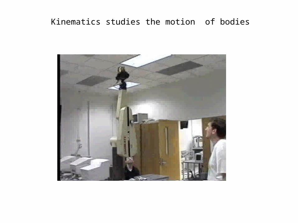
Kinematics studies the motion of bodies
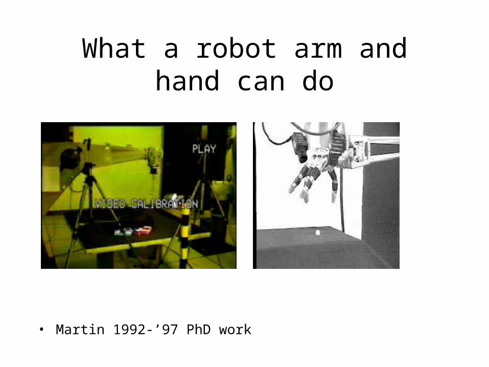
What a robot arm and hand can do
• Martin 1992-’97 PhD work

What a robot arm and hand can do
• Camilo 2011-? PhD work

Robotics field . .
• 6 Million mobile robots– From $100 roomba to $millions Mars rovers
• 1 million robot arms– Usually $20,000-100,000, some millions
• Value of industrial robotics: $25 billion• Arms crucial for these industries:
– Automotive (Welding, painting, some assembly)
– Electronics (Placing tiny components on PCB)
– General: Pack boxes, move parts from conveyor to machines
http://www.youtube.com/watch?v=DG6A1Bsi-lg

An classic arm - The PUMA 560
The PUMA 560 has SIX revolute jointsA revolute joint has ONE degree of freedom ( 1 DOF) that is defined by its angle
1
23
4
There are two more joints on the end effector (the gripper)

An modern arm - The Barrett WAM
• The WAM has SEVEN revolute joints.
• Similar motion (Kinematics) to human

UA Robotics Lab platform2 arm mobile manipulator
• 2 WAM arms, steel cable transmission and drive• Segway mobile platform• 2x Quad core computer platform.• Battery powered, 4h run time.

Robotics challenges
•
Navigation ‘05Manipulation ‘11-14
Humanoids ’12-

Build or buy?
• Off the shelf kits:
• Build your own:
Lego Lynxmotion

Mathematical modeling
Strategy:
1. Model each joint separately
2. Combine joints and linkage lengths
RobotAbstract model
http://www.societyofrobots.com/robot_arm_tutorial.shtml

Other basic joints
Spherical Joint3 DOF ( Variables - 1, 2, 3)
Revolute Joint1 DOF ( Variable - )
Prismatic Joint1 DOF (linear) (Variables - d)

ExampleMatlab robot
Successive translation and rotation
% robocop Simulates a 3 joint robot
function Jpos = robocop(theta1,theta2,theta3,L1,L2,L3,P0)
Rxy1 = [cos(theta1) sin(theta1) 0-sin(theta1) cos(theta1) 00 0 1];
Rxz2 = [cos(theta2) 0 sin(theta2)0 1 0-sin(theta2) 0 cos(theta2)];
Rxz3 = [cos(theta3) 0 sin(theta3)0 1 0-sin(theta3) 0 cos(theta3)];
P1 = P0 + Rxy1*[L1 0 0]';
P2 = P1 + Rxy1*Rxz2*[L2 0 0]';
P3 = P2 + Rxy1*Rxz2*Rxz3*[L3 0 0]';
Jpos = [P0 P1 P2 P3];

Problem: Lots of coordinate frames to calibrate
Robot– Base frame
– End-effector frame
– Object

Problem: Lots of coordinate frames to calibrate
Camera– Center of projection
– Different models
Robot– Base frame
– End-effector frame
– Object

We are interested in two kinematics topics
Forward Kinematics (angles to position)What you are given: The length of each link
The angle of each joint
What you can find: The position of any point (i.e. it’s (x, y, z) coordinates
Inverse Kinematics (position to angles)What you are given: The length of each link
The position of some point on the robot
What you can find: The angles of each joint needed to obtain that position

X1
Y1
N
O
VXY
X0
Y0
VNO
P
O
N
y
x
Y
XXY
V
V
cosθsinθ
sinθcosθ
P
P
V
VV
(VN,VO)
In other words, knowing the coordinates of a point (VN,VO) in some coordinate frame (NO) you can find the position of that point relative to your original coordinate frame (X0Y0).
(Note : Px, Py are relative to the original coordinate frame. Translation followed by rotation is different than rotation followed by translation.)
Translation along P followed by rotation by
Change Coordinate Frame

O
N
y
x
Y
XXY
V
V
cosθsinθ
sinθcosθ
P
P
V
VV
HOMOGENEOUS REPRESENTATIONPutting it all into a Matrix
1
V
V
100
0cosθsinθ
0sinθcosθ
1
P
P
1
V
VO
N
y
xY
X
1
V
V
100
Pcosθsinθ
Psinθcosθ
1
V
VO
N
y
xY
X
What we found by doing a translation and a rotation
Padding with 0’s and 1’s
Simplifying into a matrix form
100
Pcosθsinθ
Psinθcosθ
H y
x
Homogenous Matrix for a Translation in XY plane, followed by a Rotation around the z-axis

Rotation Matrices in 3D – OK,lets return from homogenous repn
100
0cosθsinθ
0sinθcosθ
R z
cosθ0sinθ
010
sinθ0cosθ
Ry
cosθsinθ0
sinθcosθ0
001
R z
Rotation around the Z-Axis
Rotation around the Y-Axis
Rotation around the X-Axis

1000
0aon
0aon
0aon
Hzzz
yyy
xxx
Homogeneous Matrices in 3D
H is a 4x4 matrix that can describe a translation, rotation, or both in one matrix
Translation without rotation
1000
P100
P010
P001
Hz
y
x
P
Y
X
Z
Y
X
Z
O
N
A
O
N
ARotation without translation
Rotation part: Could be rotation around z-axis, x-axis, y-axis or a combination of the three.

1
A
O
N
XY
V
V
V
HV
1
A
O
N
zzzz
yyyy
xxxx
XY
V
V
V
1000
Paon
Paon
Paon
V
Homogeneous Continued….
The (n,o,a) position of a point relative to the current coordinate frame you are in.
The rotation and translation part can be combined into a single homogeneous matrix IF and ONLY IF both are relative to the same coordinate frame.
xA
xO
xN
xX PVaVoVnV

Finding the Homogeneous MatrixEX.
Y
X
Z
J
I
K
N
OA
T
P
A
O
N
W
W
W
A
O
N
W
W
W
K
J
I
W
W
W
Z
Y
X
W
W
W Point relative to theN-O-A frame
Point relative to theX-Y-Z frame
Point relative to theI-J-K frame
A
O
N
kkk
jjj
iii
k
j
i
K
J
I
W
W
W
aon
aon
aon
P
P
P
W
W
W
1
W
W
W
1000
Paon
Paon
Paon
1
W
W
W
A
O
N
kkkk
jjjj
iiii
K
J
I

Y
X
Z
J
I
K
N
OA
TP
A
O
N
W
W
W
k
J
I
zzz
yyy
xxx
z
y
x
Z
Y
X
W
W
W
kji
kji
kji
T
T
T
W
W
W
1
W
W
W
1000
Tkji
Tkji
Tkji
1
W
W
W
K
J
I
zzzz
yyyy
xxxx
Z
Y
X
Substituting for
K
J
I
W
W
W
1
W
W
W
1000
Paon
Paon
Paon
1000
Tkji
Tkji
Tkji
1
W
W
W
A
O
N
kkkk
jjjj
iiii
zzzz
yyyy
xxxx
Z
Y
X

1
W
W
W
H
1
W
W
W
A
O
N
Z
Y
X
1000
Paon
Paon
Paon
1000
Tkji
Tkji
Tkji
Hkkkk
jjjj
iiii
zzzz
yyyy
xxxx
Product of the two matrices
Notice that H can also be written as:
1000
0aon
0aon
0aon
1000
P100
P010
P001
1000
0kji
0kji
0kji
1000
T100
T010
T001
Hkkk
jjj
iii
k
j
i
zzz
yyy
xxx
z
y
x
H = (Translation relative to the XYZ frame) * (Rotation relative to the XYZ frame) * (Translation relative to the IJK frame) * (Rotation relative to the IJK frame)

The Homogeneous Matrix is a concatenation of numerous translations and rotations
Y
X
Z
J
I
K
N
OA
TP
A
O
N
W
W
W
One more variation on finding H:
H = (Rotate so that the X-axis is aligned with T)
* ( Translate along the new t-axis by || T || (magnitude of T))
* ( Rotate so that the t-axis is aligned with P)
* ( Translate along the p-axis by || P || )
* ( Rotate so that the p-axis is aligned with the O-axis)
This method might seem a bit confusing, but it’s actually an easier way to solve our problem given the information we have. Here is an example…

F o r w a r d K i n e m a t i c s

The Situation:You have a robotic arm that
starts out aligned with the xo-axis.You tell the first link to move by 1 and the second link to move by 2.
The Quest:What is the position of the
end of the robotic arm?
Solution:1. Geometric Approach
This might be the easiest solution for the simple situation. However, notice that the angles are measured relative to the direction of the previous link. (The first link is the exception. The angle is measured relative to it’s initial position.) For robots with more links and whose arm extends into 3 dimensions the geometry gets much more tedious.
2. Algebraic Approach Involves coordinate transformations.

X2
X3Y2
Y3
1
2
3
1
2 3
Example Problem: You are have a three link arm that starts out aligned in the x-axis.
Each link has lengths l1, l2, l3, respectively. You tell the first one to move by 1
, and so on as the diagram suggests. Find the Homogeneous matrix to get the position of the yellow dot in the X0Y0 frame.
H = Rz(1 ) * Tx1(l1) * Rz(2 ) * Tx2(l2) * Rz(3 )
i.e. Rotating by 1 will put you in the X1Y1 frame. Translate in the along the X1 axis by l1. Rotating by 2 will put you in the X2Y2 frame. and so on until you are in the X3Y3 frame.
The position of the yellow dot relative to the X3Y3 frame is(l1, 0). Multiplying H by that position vector will give you the coordinates of the yellow point relative the the X0Y0 frame.
X1
Y1
X0
Y0

Slight variation on the last solution:Make the yellow dot the origin of a new coordinate X4Y4 frame
X2
X3Y2
Y3
1
2
3
1
2 3
X1
Y1
X0
Y0
X4
Y4
H = Rz(1 ) * Tx1(l1) * Rz(2 ) * Tx2(l2) * Rz(3 ) * Tx3(l3)
This takes you from the X0Y0 frame to the X4Y4 frame.
The position of the yellow dot relative to the X4Y4 frame is (0,0).
1
0
0
0
H
1
Z
Y
X
Notice that multiplying by the (0,0,0,1) vector will equal the last column of the H matrix.

More on Forward Kinematics…
Denavit - Hartenberg Parameters

Denavit-Hartenberg Notation
Z(i - 1)
X(i -1)
Y(i -1)
( i - 1)
a(i - 1 )
Z i Y i
X i a i
d i
i
IDEA: Each joint is assigned a coordinate frame. Using the Denavit-Hartenberg notation, you need 4 parameters to describe how a frame (i) relates to a previous frame ( i -1 ).
THE PARAMETERS/VARIABLES: , a , d,

The Parameters
Z(i - 1)
X(i -1)
Y(i -1)
( i - 1)
a(i - 1 )
Z i Y i
X i a i d i
i
You can align the two axis just using the 4 parameters
1) a(i-1)
Technical Definition: a(i-1) is the length of the perpendicular between the joint axes. The joint axes is the axes around which revolution takes place which are the Z(i-1) and Z(i) axes. These two axes can be viewed as lines in space. The common perpendicular is the shortest line between the two axis-lines and is perpendicular to both axis-lines.

a(i-1) cont...
Visual Approach - “A way to visualize the link parameter a(i-1) is to imagine an expanding cylinder whose axis is the Z(i-1) axis - when the cylinder just touches the joint axis i the radius of the cylinder is equal to a(i-1).” (Manipulator Kinematics)
It’s Usually on the Diagram Approach - If the diagram already specifies the various coordinate frames, then the common perpendicular is usually the X(i-1) axis. So a(i-1) is just the displacement along the X(i-1) to move from the (i-1) frame to the i frame.
If the link is prismatic, then a(i-1) is a variable, not a parameter. Z(i - 1)
X(i -1)
Y(i -1)
( i - 1)
a(i - 1 )
Z i Y i
X i a i d i
i

2) (i-1)
Technical Definition: Amount of rotation around the common perpendicular so that the joint axes are parallel.
i.e. How much you have to rotate around the X(i-1) axis so that the Z(i-1) is pointing in
the same direction as the Zi axis. Positive rotation follows the right hand rule.
3) d(i-1)
Technical Definition: The displacement along the Zi axis needed to align the a(i-1) common perpendicular to the ai common perpendicular.
In other words, displacement along the
Zi to align the X(i-1) and Xi axes.
4) i
Amount of rotation around the Zi axis needed to align the X(i-1) axis with the Xi
axis.
Z(i - 1)
X(i -1)
Y(i -1)
( i - 1)
a(i - 1 )
Z i Y i
X i a i d i
i

The Denavit-Hartenberg Matrix
1000
cosαcosαsinαcosθsinαsinθ
sinαsinαcosαcosθcosαsinθ
0sinθcosθ
i1)(i1)(i1)(ii1)(ii
i1)(i1)(i1)(ii1)(ii
1)(iii
d
d
a
Just like the Homogeneous Matrix, the Denavit-Hartenberg Matrix is a transformation matrix from one coordinate frame to the next. Using a series of D-H Matrix multiplications and the D-H Parameter table, the final result is a transformation matrix from some frame to your initial frame.
Z(i -
1)
X(i -1)
Y(i -1)
( i -
1)
a(i -
1 )
Z i Y
i X
i
a
i
d
i
i
Put the transformation here

3 Revolute Joints
i (i-1) a(i-1) di
i
0 0 0 0 0
1 0 a0 0 1
2 -90 a1 d2 2
Z0
X0
Y0
Z1
X2
Y1
Z2
X1
Y2
d2
a0 a1
Denavit-Hartenberg Link Parameter Table
Notice that the table has two uses:
1) To describe the robot with its variables and parameters.
2) To describe some state of the robot by having a numerical values for the variables.

Z0
X0
Y0
Z1
X2
Y1
Z2
X1
Y2
d2
a0 a1
i (i-1) a(i-1) di
i
0 0 0 0 0
1 0 a0 0 1
2 -90 a1 d2 2
1
V
V
V
TV2
2
2
000
Z
Y
X
ZYX T)T)(T)((T 12
010
Note: T is the D-H matrix with (i-1) = 0 and i = 1.

1000
0100
00cosθsinθ
00sinθcosθ
T 00
00
0
i (i-1) a(i-1) di
i
0 0 0 0 0
1 0 a0 0 1
2 -90 a1 d2 2
This is just a rotation around the Z0 axis
1000
0000
00cosθsinθ
a0sinθcosθ
T 11
011
01
1000
00cosθsinθ
d100
a0sinθcosθ
T22
2
122
12
This is a translation by a0 followed by a rotation around the Z1 axis
This is a translation by a1 and then d2 followed by a rotation around the X2 and Z2 axis
T)T)(T)((T 12
010

I n v e r s e K i n e m a t i c s
From Position to Angles

A Simple Example
1
X
Y
S
Revolute and Prismatic Joints Combined
(x , y)
Finding :
)x
yarctan(θ
More Specifically:
)x
y(2arctanθ arctan2() specifies that it’s in the
first quadrant
Finding S:
)y(xS 22

2
1
(x , y)
l2
l1
Inverse Kinematics of a Two Link Manipulator
Given: l1, l2 , x , y
Find: 1, 2
Redundancy:A unique solution to this problem
does not exist. Notice, that using the “givens” two solutions are possible. Sometimes no solution is possible.
(x , y)l2
l1
l2
l1

The Geometric Solution
l1
l22
1
(x , y) Using the Law of Cosines:
21
22
21
22
21
22
21
22
212
22
122
222
2arccosθ
2)cos(θ
)cos(θ)θ180cos(
)θ180cos(2)(
cos2
ll
llyx
ll
llyx
llllyx
Cabbac
2
2
22
2
Using the Law of Cosines:
x
y2arctanα
αθθ
yx
)sin(θ
yx
)θsin(180θsin
sinsin
11
22
2
22
2
2
1
l
c
C
b
B
x
y2arctan
yx
)sin(θarcsinθ
22
221
l
Redundant since 2 could be in the first or fourth quadrant.
Redundancy caused since 2 has two possible values

21
22
21
22
2
2212
22
1
211211212
22
1
211212
212
22
12
1211212
212
22
12
1
2222
2
yxarccosθ
c2
)(sins)(cc2
)(sins2)(sins)(cc2)(cc
yx)2((1)
ll
ll
llll
llll
llllllll
The Algebraic Solution
l1
l22
1
(x , y)
21
21211
21211
1221
11
θθθ(3)
sinsy(2)
ccx(1)
)θcos(θc
cosθc
ll
ll
Only Unknown
))(sin(cos))(sin(cos)sin(
))(sin(sin))(cos(cos)cos(
:
abbaba
bababa
Note

X2
X3Y2
Y3
r1
r2
r3
1
2 3
X1
Y1
X0
Y0
X4
Y4
We model forward kinematics asH = Ry(r1 ) * Tx1(l1) * Rz(r2 ) * Tx2(l2) * Rz(r3 ) * Tx3(l3)
Now given desired Cartesian position [X,Y,Z] solve numerically for the corresponding joint angles [r1 r2 r3] :
1
0
0
0
H
1
Z
Y
X
),()( lrrf
)(0 rf
1
Z
Y
X
The Numeric solution

X2
X3Y2
Y3
r1
r2
r3
1
2 3
X1
Y1
X0
Y0
X4
Y4
Function:
Jacobian J = matrix of partial derivatives:
Newton’s method:Guess initial joint angles rIterate J*dr = W-f( r ) r = r+drIf guess is close enough r converges to solution.Otherwise may diverge.
IlrrfW ),()(4 H
The Numeric solution: How to solve?Newton’s Metod
j
i
r
rf )(J
r1
1
r2
2
r3
3
X
Y
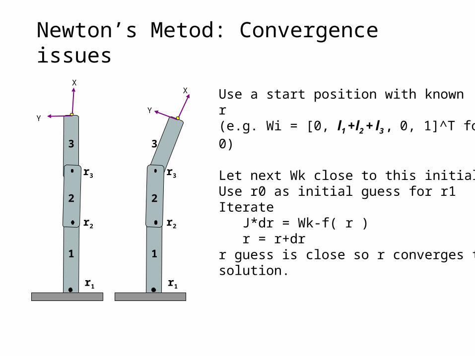
Use a start position with known W and r(e.g. Wi = [0, l1 +l2 + l3 , 0, 1]^T for r = 0)
Let next Wk close to this initial.Use r0 as initial guess for r1Iterate J*dr = Wk-f( r ) r = r+drr guess is close so r converges to solution.
Newton’s Metod: Convergence issues
r1
1
r2
2
r3
3
X
Y

r1
1
r2
2
r3
3
X
Y
To make a large movement, divide the total distance from (known) initial Wi to the new final Wf into small steps Wk e.g. on a line
•Try this in lab!
Newton’s Metod: Convergence issues
X3
r3
1
2 3
Y 1
X4
Y4
IlrrfW ),()(4 H
j
i
r
rf )(J

Resolved rate control
• Here instead of computing an inverse kinematics solution then move the robot to that point, we actually move the robot dr for every iteration in newtons method.
• Let dr 0, then we can view this as velocity control:
wtrr 1))(( J
n velovitytranslatioCartesian vw

Conclusion• Forward kinematics can be tedious for multilink arms
• Inverse kinematics can be solved algebraically or numerically. The latter is more common for complex arms or vision-guided control (later)
• Limitations: We avoided details of the various angular representations (Euler, quarternion or exponentials) and their detailed use in Kinematics. (this typically takes several weeks of course time in engineering courses)

Quick Math ReviewDot Product: Geometric Representation:
A
Bθ
cosθBABA
Unit VectorVector in the direction of a chosen vector but whose magnitude is 1.
B
BuB
y
x
a
a
y
x
b
b
Matrix Representation:
yyxxy
x
y
xbaba
b
b
a
aBA
B
Bu

Quick Matrix Review
Matrix Multiplication:
An (m x n) matrix A and an (n x p) matrix B, can be multiplied since the number of columns of A is equal to the number of rows of B.
Non-Commutative MultiplicationAB is NOT equal to BA
dhcfdgce
bhafbgae
hg
fe
dc
ba
Matrix Addition:
hdgc
fbea
hg
fe
dc
ba

Basic TransformationsMoving Between Coordinate Frames
Translation Along the X-Axis
N
O
X
Y
VNO
VXY
Px
VN
VO
Px = distance between the XY and NO coordinate planes
Y
XXY
V
VV
O
NNO
V
VV
0
PP x
P
(VN,VO)
Notation:

NX
VNO
VXY
PVN
VO
Y O
NO
O
NXXY VPV
VPV
Writing in terms of XYV NOV

X
VXY
PXY
N
VNO
VN
VO
O
Y
Translation along the X-Axis and Y-Axis
O
Y
NXNOXY
VP
VPVPV
Y
xXY
P
PP

oV
nV
θ)cos(90V
cosθV
sinθV
cosθV
V
VV
NO
NO
NO
NO
NO
NO
O
NNO
NOV
o
n Unit vector along the N-Axis
Unit vector along the N-Axis
Magnitude of the VNO vector
Using Basis VectorsBasis vectors are unit vectors that point along a coordinate axis
N
VNO
VN
VO
O
n
o

Rotation (around the Z-Axis)X
Y
Z
X
Y
N
VN
VO
O
V
VX
VY
Y
XXY
V
VV
O
NNO
V
VV
= Angle of rotation between the XY and NO coordinate axis

X
Y
N
VN
VO
O
V
VX
VY
Unit vector along X-Axis
x
xVcosαVcosαVV NONOXYX
NOXY VV
Can be considered with respect to the XY coordinates or NO coordinates
V
x)oVn(VV ONX (Substituting for VNO using the N and O components of the vector)
)oxVnxVV ONX ()(
))
)
(sinθV(cosθV
90))(cos(θV(cosθVON
ON

Similarly….
yVα)cos(90VsinαVV NONONOY
y)oVn(VV ONY
)oy(V)ny(VV ONY
))
)
(cosθV(sinθV
(cosθVθ))(cos(90VON
ON
So….
)) (cosθV(sinθVV ONY )) (sinθV(cosθVV ONX
Y
XXY
V
VV
Written in Matrix Form
O
N
Y
XXY
V
V
cosθsinθ
sinθcosθ
V
VV
Rotation Matrix about the z-axis

))(sin(cos))(sin(cos)sin(
))(sin(sin))(cos(cos)cos(
:
abbaba
bababa
Note
)c(s)s(c
cscss
sinsy
)()c(c
ccc
ccx
2211221
12221211
21211
2212211
21221211
21211
lll
lll
ll
slsll
sslll
ll
We know what 2 is from the previous slide. We need to solve for 1 . Now we have two equations and two unknowns (sin 1 and cos 1 )
2222221
1
2212
22
1122221
221122221
221
221
2211
yx
x)c(ys
)c2(sx)c(
1
)c(s)s()c(
)(xy
)c(
)(xc
slll
llllslll
lllll
sls
ll
sls
Substituting for c1 and simplifying many times
Notice this is the law of cosines and can be replaced by x2+ y2
22
222211
yx
x)c(yarcsinθ
slll
Top Related