


Languages
Pages
Legal


i
Risk Assessment for Floods Due to Precipitation Exceeding Drainage Capacity November 2006 Umut Karamahmut
Faculty of Civil Engineering and Geosciences
ii
i. Abstract
Studies on flood risk modeling were concentrated on floods caused by breaches of dunes
and levees. Another kind of flood which was not considered in risk calculations was
floods due to precipitation exceeding drainage capacity of low lands. As a result of the
increase in the extreme precipitation events due to climate change and increased land
value, the risk due to this kind of floods increased considerably, and must be calculated.
This study aims to investigate and improve current situation in risk assessment of floods
due to rainfall exceeding capacity of the drainage system of polders. In order to achieve
this, commercially available models were investigated to find out if any of them are
capable of calculating risk for these floods. Research on existing models showed that
none of these models were applicable for this problem.
Calculation of risk for this kind of floods comes along with massive work load. In order
to able to carry on these calculations the problem must be simplified by eliminating one o
the parameters. In order to validate this simplification, correlation between two flood
parameters namely, flood depth and flood duration were proved.
Finally applicability of a risk analysis tool for this problem was investigated with a case
study on Polder Berkel. Results showed that risk analysis methods were applicable to the
case but some improvements were necessary.

iii
ii. Acknowledgments
I would like to express my thanks to Elgard van Leeuwen and Olivier Hoes for their
constant supervision and valuable comments through out my studies.
I also would like to thank to Nick van de Giesen, Elgard van Leeuwen and Olivier Hoes
for taking part in my graduation committee.
I appreciate contributions of Colin Green and Edmund Penning-Rowsell from Flood
Hazard Research Centre, Middlesex University, United Kingdom, Roy Leigh from
Natural Hazards Research Center, Macquarie University, Australia and Duncan Faulkner
from JBA Consulting – Engineers & Scientists and all WL|Delft Hydraulics employees
who were always there to answer my questions and support me.
The last but not the least I would like to thank to my family and friends, without their
support none of this would be possible. Especially to my mother, for holding up to life.
iv
Table of Contents
1. Introduction:................................................................................................................ 1
1.1. Flooding ................................................................................................................... 1 1.2. Problem.................................................................................................................... 3 1.3. Objectives ................................................................................................................ 4 1.4. Report structure........................................................................................................ 5
2. Research on existing flood risk models ...................................................................... 6 2.1. Introduction.............................................................................................................. 6 2.2. Basics of flood risk estimation................................................................................. 7 2.3. Existing Flood Loss Estimation Models ................................................................ 10 2.4. Evaluation .............................................................................................................. 25 2.5. Conclusion ............................................................................................................. 27
3. Correlation of flood depth and duration for different soil types............................... 29 3.1. Introduction............................................................................................................ 29 3.2. Methodology.......................................................................................................... 30 3.3. Model Schematization ........................................................................................... 31 3.4. Model Data............................................................................................................. 32 3.5. Post processing of simulation results..................................................................... 37 3.6. Results.................................................................................................................... 41 3.7. Evaluation & Conclusion....................................................................................... 45
4. Case Study: Polder Berkel ........................................................................................ 46 4.1. Introduction............................................................................................................ 46 4.2. Polder Berkel ......................................................................................................... 47 4.3. WB21 Method........................................................................................................ 50 4.4. Risk Model............................................................................................................. 58 4.5. Case Discussion & Comparison............................................................................. 64 4.6. Conclusions............................................................................................................ 69
5. Conclusions & Recommendations............................................................................ 70 5.1. Conclusions............................................................................................................ 71 5.2. Recommendations.................................................................................................. 73
6. References................................................................................................................. 75 7. Appendix................................................................................................................... 77
v
List of Figures
Figure 1-1 Inundation map of Netherlands without dikes, dunes and pumping stations... 1 Figure 2-1 Water Surface Profiles Plot............................................................................. 12 Figure 2-2Depth-Percent Damage Functions For Apartments ........................................ 13 Figure 2-3 Scale levels of damage evaluation .................................................................. 14 Figure 2-4Property Damages Output of MDSF................................................................ 18 Figure 2-5Components of FloodAUS............................................................................... 23 Figure 2-6 3-D representation of flood extend ................................................................. 24 Figure 3-1SOBEK Model Schematization........................................................................ 31 Figure 3-2Ernst Drainage Calculation Parameters ........................................................... 33 Figure 3-3Drainage Coefficients Input Screen ................................................................. 34 Figure 3-4Visual Basic script for determination of events ............................................... 38 Figure 3-5Output file view of the script ........................................................................... 39 Figure 3-6Depth – Duration graph for Sand Average (average) ...................................... 41 Figure 3-7Depth – Duration graph for Sand Average (maximum)................................... 42 Figure 3-8Trend lines of different soil types (average) .................................................... 43 Figure 3-9Trend lines of different soil types (maximum) ............................................... 43 Figure 4-1Sub-polders and target elevations .................................................................... 48 Figure 4-2Satellite Image of Polder Berkel ...................................................................... 49 Figure 4-3Damage Function for Greenhouses and Urban Areas...................................... 55 Figure 4-4SOBEK Model for Polder Berkel .................................................................... 56 Figure 4-5WB21 Script Output File View........................................................................ 57 Figure 4-6Digital Elevation Map Figure 4-7Water Compartments................... 59 Figure 4-8 Land Use Map ................................................................................................. 60 Figure 4-9Risk Model Damage Functions........................................................................ 61 Figure 4-10Hymstat Output .............................................................................................. 62 Figure 4-11Risk Map ........................................................................................................ 63

vi
List of Tables
Table 2-1 Damage categories.............................................................................................. 8 Table 2-2 Inundation parameters ........................................................................................ 9 Table 2-3Stage-Damage relations for residential properties ............................................ 19 Table 2-4Damage categories for commercial properties .................................................. 20 Table 2-5Stage-Damage relations for commercial properties .......................................... 21 Table 2-6Coverage of existing flood loss estimation models........................................... 25 Table 3-1Unpaved node parameters ................................................................................. 32 Table 3-2Ernst coefficients for different soil types .......................................................... 35 Table 3-3Coefficient of Determination for different soil types ........................................ 44 Table 3-4Correlation Coefficient for different soil types ................................................. 44 Table 4-1Maximum damage per hectare for different land use........................................ 51 Table 4-2Workability coefficients for seasons and soil types for grassland .................... 52 Table 4-3Workability coefficients for seasons and soil types for agriculture .................. 53 Table 4-4Workability coefficients for high quality agriculture and horticulture ............. 54 Table 4-5Drowning coefficients ....................................................................................... 54 Table 4-6Risk calculated by Risk Model and WB21 method........................................... 65 Table 4-7Monetary Difference and Ratio between Risk Model and WB21 method........ 66

1
1. Introduction:
1.1. Flooding
The Netherlands, being located in delta of The Rhine, The Meuse and The Scheldt, has a
long history in coping with floods. As a result of past water management practices, land
reclamation and subsidence, higher percentage of The Netherlands lies on large flat
plains under mean sea level. Thus they require both protection from sea and constant
drainage of the excess water out of the polders. (See Figure 1.1)
Figure 1-1 Inundation map of The Netherlands without dikes, dunes and pumping stations
Source: Hoes, 2005

2
Studies on flood protection and flood damage modeling were mostly concentrated on the
floods caused by breaches of dunes and levees since a flood resulting from these would
be sudden and extensive and combined effects may be catastrophic but recently attention
was also given to floods due to precipitation exceeding capacity of the drainage canals
and pumping stations of polders. This kind of flood is neither life threatening nor as
catastrophic as the floods due to breaches of dunes and levees but they might occur rather
frequently resulting in substantial losses. (Hoes, 2005)
Both total annual precipitation and extreme precipitation events are following an
increasing trend especially in the last two decades. It is believed that this trend will
continue due to climate change and further more floods events will be more frequent
because of sea level rise and subsidence.(IPCC, 2001) Increase in frequency and
magnitude of these events once again showed that regional rainfall induced floods can
not always be prevented. On the other hand possible losses due to these events are also
escalating because of increasing value of land and on going urbanization. In order to
avoid these losses many water systems must be upgraded. Risk of flooding must be
calculated in order to asses the feasibility of the measures taken to upgrade these systems.
3
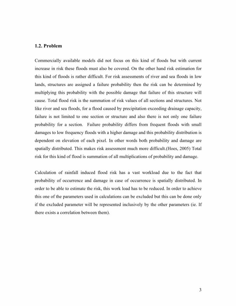
1.2. Problem
Commercially available models did not focus on this kind of floods but with current
increase in risk these floods must also be covered. On the other hand risk estimation for
this kind of floods is rather difficult. For risk assessments of river and sea floods in low
lands, structures are assigned a failure probability then the risk can be determined by
multiplying this probability with the possible damage that failure of this structure will
cause. Total flood risk is the summation of risk values of all sections and structures. Not
like river and sea floods, for a flood caused by precipitation exceeding drainage capacity,
failure is not limited to one section or structure and also there is not only one failure
probability for a section. Failure probability differs from frequent floods with small
damages to low frequency floods with a higher damage and this probability distribution is
dependent on elevation of each pixel. In other words both probability and damage are
spatially distributed. This makes risk assessment much more difficult.(Hoes, 2005) Total
risk for this kind of flood is summation of all multiplications of probability and damage.
Calculation of rainfall induced flood risk has a vast workload due to the fact that
probability of occurrence and damage in case of occurrence is spatially distributed. In
order to be able to estimate the risk, this work load has to be reduced. In order to achieve
this one of the parameters used in calculations can be excluded but this can be done only
if the excluded parameter will be represented inclusively by the other parameters (ie. If
there exists a correlation between them).
4
1.3. Objectives
This study aims to investigate and improve current situation in determination of risk of
floods in low lands due to rainfall exceeding drainage capacity. In order to achieve this,
following objectives will be studied through out the study.
- To figure out if any of the commercially available models are capable of solving this
problem considering the different nature of rainfall induced floods in low lands.
- To prove the correlation between flood depth and flood duration. This correlation is
rather important because proof of such a correlation will allow us to eliminate one of
these parameters, reducing the vast workload and enabling us to calculate risk.
- To investigate the applicability of a new risk analysis tool for calculation of risk for
rainfall induced regional floods in low lands.

5
1.4. Report structure The above mentioned objectives were addressed in different chapters as described below.
In chapter two current practices and models in three countries namely as United
Kingdom, United States and Australia were investigated in order to figure out if any of
the commercially available models were capable of solving this problem. Existing models
were not capable of carrying out this calculation.
In the third chapter correlation between flood depth and duration was proved by
simulating water levels for a long enough period for 12 most common soil types in
Netherlands.
In the fourth chapter a case study was carried out in order to investigate the applicability
of a new risk analysis tool for calculation of risk for rainfall induced regional floods.
Annual average risk calculated by this tool was compared with the risk value calculated
by a traditional damage assessment method. Rationales behind risk calculation were
investigated in order to reach a balance between workload and accuracy.
The study was concluded and recommendations for further studies were given in chapter
five.

6
2. Research on existing flood risk models
2.1. Introduction
In this chapter applicability of existing flood risk models to the case of floods in low
lands due to precipitation exceeding drainage capacity will be investigated by studying
working principles of 6 models used in 3 countries. These models and countries are as
follows.
United States : - HAZUS - MH
- HEC-FDA
United Kingdom : - ESTDAM
- MDSF
Australia : - ANUFLOOD
- FloodAUS
Studies showed that current flood risk modeling practices in different countries are not
applicable for modeling of flood risk due to high precipitation which exceeds the capacity
of the drainage system. Reasons why they are not applicable will be mentioned further
on.
In following section basics of flood risk analysis and common practices will be
mentioned. In third section an overview of the flood risk estimation methods used in
different countries will be given. Evaluation of applicability of these methods to the case
of concern will be carried out in forth section and conclusions will be given in fifth
section.

7
2.2. Basics of flood risk estimation
In this section, common practices used in different models thus different countries will be
mentioned.
In all of the models flood risk is defined as the sum of multiplication of damage in case of
occurrence of events and probabilities that those events will occur. In order to calculate
risk inundation maps with known occurrence probabilities were used.
Flood damage and risk were categorized in different ways. These are as follows.
2.2.1. Type of flooding
Damage and risk can be categorized according to the source of flooding. A flood might
be caused by sea, river or precipitation. The source of flooding effects damage in various
ways. For example a sea flood will have extra damage on agricultural fields due to
salination. Also source of flooding changes calculation method for risk of flooding.
2.2.2. Categorization according to consequences
In general there exists there different criteria to classify damages caused by natural
disasters. First division is between tangible and intangible damages. Tangible damages
are those which can be described in monetary units, thus they can be evaluated and
compared. Damages to buildings or contents of buildings can be an example to tangible
damages. Intangible damages are the ones which is difficult to describe in economic
terms, for example physical and psychological traumas. Recently more studies are being
carried out for quantification of intangible damages. An exemplary is “Anxiety-
Productivity and Income Interrelationship Approach” (API). This approach is explained
in detail elsewhere (Lekuthai, Vongvisessomjai, 2001)

8
Another division is direct and indirect losses. Direct losses are caused by physical contact
of flood water while indirect losses are caused through interruption and disruption of
economic and social activities as a consequence of direct flood damages. (Dutta et
al.,2001) Destruction of buildings is a direct damage while production loss is an indirect
damage.
Direct, indirect and tangible, intangible damages can further be divided as primary and
secondary damages. The table below can be an example for the division of damages
according to the above mentioned criteria.
Table 2-1 Damage categories
Category Tangible Intangible
Direct Capital Loss (houses, crops, cars, factory buildings)
Victims, ecosystems, pollution, monuments, culture loss Primary
Indirect Production losses, income loss Social disruption, emotional damage
Secondary Production losses outside the flood area, unemployment, migration, inflation
Emotional damage, damage to ecosystem outside the flood area
Induced Costs for relief aid Evacuation stress Source: K.M. de Bruijn, 2005, pg. 41.
Ideally all these kinds of damages should be considered in estimations but in practice this
is impossible. In most of the studies damages are restricted to primary tangible damages
and part of the production losses by companies and agriculture. This is due to the
complexity of calculating secondary tangible or intangible damages. These damages are
introduced in bulk form by multiplying the primary tangible damage by a factor which is
dependent to the properties of the region.
9
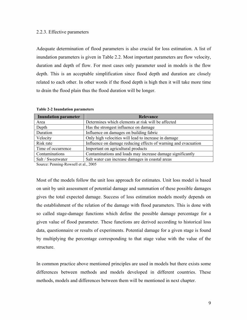
2.2.3. Effective parameters
Adequate determination of flood parameters is also crucial for loss estimation. A list of
inundation parameters is given in Table 2.2. Most important parameters are flow velocity,
duration and depth of flow. For most cases only parameter used in models is the flow
depth. This is an acceptable simplification since flood depth and duration are closely
related to each other. In other words if the flood depth is high then it will take more time
to drain the flood plain thus the flood duration will be longer.
Table 2-2 Inundation parameters
Inundation parameter Relevance Area Determines which elements at risk will be affected Depth Has the strongest influence on damage Duration Influence on damages on building fabric Velocity Only high velocities will lead to increase in damage Risk rate Influence on damage reducing effects of warning and evacuation Time of occurrence Important on agricultural products Contaminations Contaminations and loads may increase damage significantly Salt / Sweetwater Salt water can increase damages in coastal areas Source: Penning-Rowsell et al., 2005
Most of the models follow the unit loss approach for estimates. Unit loss model is based
on unit by unit assessment of potential damage and summation of these possible damages
gives the total expected damage. Success of loss estimation models mostly depends on
the establishment of the relation of the damage with flood parameters. This is done with
so called stage-damage functions which define the possible damage percentage for a
given value of flood parameter. These functions are derived according to historical loss
data, questionnaire or results of experiments. Potential damage for a given stage is found
by multiplying the percentage corresponding to that stage value with the value of the
structure.
In common practice above mentioned principles are used in models but there exists some
differences between methods and models developed in different countries. These
methods, models and differences between them will be mentioned in next chapter.

10
2.3. Existing Flood Loss Estimation Models
Different damage assessment models were developed in different countries. These
models are mainly built for cost efficiency studies of flood mitigation measures or
assessment of risk for insurance purposes. In this section different models used in United
States, Australia and United Kingdom will be mentioned.
2.3.1. United States:
In United States a variety of organizations are involved in damage assessment and
prevention. As a result no standard method has been developed. (K. de Bruijn, 2001)
There are two commonly used models, HEC-FDA and HAZUS-MH.
2.3.1.1. HAZUS-MH:
The name of the model stands for “Hazard United States – Multiple Hazards”. HAZUS
was initially developed for assessment of earthquake damages by Federal Emergency
Management Agency (FEMA). Later FEMA released a newer version by which a variety
of hazards, including floods, and their risk assessments may be investigated.
HAZUS is a flexible program that allows performing the analysis on different levels
depending on resources and analysis needs. Level 1 uses available hazard and inventory
data provided by HAZUS-MH, limited additional data is required in this level. Level 2
analyses require local data which is readily available for most of the cases or can be
converted to model requirements easily by Flood Information Tool (FIT, a built in
function of the model for conversion of data). Level 3 involves adjustment of built in loss
estimation models.

11
Loss estimate analysis can be run for three different analysis options. These options are;
(1) multiple return periods of 10, 50, 100, 200 and 500 years, (2) a user defined single
frequency or (3) annualized loss. For comparison of flood mitigation measures third
option will be most adequate. (FEMA, 2004)
Although the model gives a quick estimate of the possible damage, results will not be
accurate enough unless the model is run on third level, which requires aggregation of
detailed local data and adjustment of loss estimate models.
2.3.1.2. HEC-FDA:
In United States, US Army Corps of Engineers (USACE) has nationwide responsibilities
on water resources planning and management. (Dutta et al.,2001) Thus for flood
mitigation measures USACE produced its own guidelines namely as the National
Economic Development Procedures (USACE,1988) and The Hydrologic Engineering
Center (HEC) designed the Hydrologic Engineering Center’s Flood Damage Analysis
(HEC-FDA) program in order to assist risk-based analysis methods for flood damage
reduction studies as required by USACE.
HEC-FDA uses Monte Carlo simulation, a numerical model that computes the expected
value of damage while explicitly accounting uncertainties in basic functions. It can
quantify the uncertainty in discharge – frequency, stage – discharge, geotechnical levee
failure and stage – damage functions and incorporate these into economic and
performance analysis of alternative flood damage reduction plans. Evaluations are carried
on in terms of expected annual damage equivalent annual damage or project
performance. (USACE, 1998)

12
Model uses water surface profiles and depth damage functions for calculating damage
and risk.
Water surface profiles can be discharge or stage based. A data set must contain eight
profiles. These are defined as 0.50, 0.20, 0.10, 0.04, 0.02, 0.01, 0.004 and 0.002
exceeding probability flood events. Profiles can be used for developing with or without
project condition functions. They are also used to from stage-damage functions. An
example plot of water surface profiles was given in Figure 2.1. (Burnham, 1997)
Figure 2-1 Water Surface Profiles Plot
Depth-percent damage functions can be assigned for each occupancy type. Program
allows user to define three types of depth-damage functions namely as Structure, Content
and Other. These functions can be calculated according to historical loss data,
questionnaire or experimental results. Some depth-percentage damage functions used in a
case is given below. (See Figure 2.2)
The methodology adopted is very comprehensive for estimation of damage to urban
buildings and to agriculture. However no specific methods have been developed for
estimation of damage to lifeline systems and indirect losses such as interruption losses.
(Dutta et al., 2001)

13
Figure 2-2Depth-Percent Damage Functions For Apartments (Left: structure, Right: Content)
2.3.2. United Kingdom:
In United Kingdom it is mandatory to use a standard approach for flood damage
assessment for local authorities which want the assistance of central government with
flood mitigation measures. Flood Hazard Research Center (FHRC) in Middlesex
University had been leading the studies for development of flood damage estimation
methodologies on UK. (Dutta et al., 2001). FHRC published 4 manuals presenting results
of their studies. The “Blue Manuel” (Penning-Rowsell and Chatterton, 1977) covers
assessment techniques and provides a range of depth-damage data. The “Red Manuel”
(Parker et al., 1987) provides depth-damage data and assessment methods for common
indirect losses and direct losses except the residential losses were also covered in this
manual. The “Yellow Manual” (Penning-Rowsell et al., 1992) covers the effects of
coastal erosion and assessment of environmental effects of floods. Finally FHRC
14
published the “Multi-Coloured Manual” (Penning-Rowsell et al., 2003). This manual is
called “Multi-Coloured” since it combines the techniques mentioned in previous
manuals. It covers flood alleviation benefits, indirect benefits and coast protection and
sea defense benefits in an improved and updated manner.
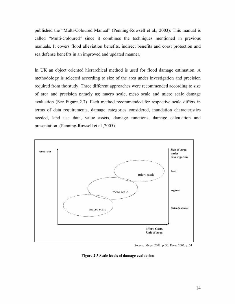
In UK an object oriented hierarchical method is used for flood damage estimation. A
methodology is selected according to size of the area under investigation and precision
required from the study. Three different approaches were recommended according to size
of area and precision namely as; macro scale, meso scale and micro scale damage
evaluation (See Figure 2.3). Each method recommended for respective scale differs in
terms of data requirements, damage categories considered, inundation characteristics
needed, land use data, value assets, damage functions, damage calculation and
presentation. (Penning-Rowsell et al.,2005)
Source: Meyer 2001, p. 30; Reese 2003, p. 54
Accuracy
Effort, Costs/ Unit of Area
macro scale
micro scale
meso scale
Size of AreaunderInvestigation
local
regional
(inter-)national
Figure 2-3 Scale levels of damage evaluation

15
It can be observed that in United Kingdom damage functions published in the “Multi-
Coloured Manuel” from FHRC build the basis of damage evaluation studies. For small
scale project appraisals the full detail of the database is used. For meso and macro scales
more aggregated damage functions are used. (Penning-Rowsell et al.,2005) This set
provides synthetically derived depth-damage functions for 100 residential and more then
10 non-residential property types.
For residential flats, first a definition and inventory of this standard property type is done.
Secondly, for each of its typical building fabric and inventory components the monetary
value is determined. Thirdly, expert assessors estimate the susceptibility of each item to
inundation depth so depth-damage functions can be constructed.
For non-residential properties surveys are carried out, in which responsible persons in
each firm are asked about the value of assets at risk and susceptibility of these assets to
inundation depth. From survey results average depth-damage curves per square meter of
property are derived for different economic branches. (Penning Rowsell et al., 2003)
These damage functions not only consider the inundation depth but also they consider
duration of flooding (i.e. more or less than 12 hours), coastal flood or not (i.e. salt or
fresh water), if a warning more than two hours is received.
Two models used in United Kingdom will be mentioned briefly.

16
2.3.2.1. ESTDAM:
ESTDAM non-GIS based model developed by FHRC. It is mostly used in micro scale
studies for project appraisals. It applies a property by property approach and it is matched
with the standard depth-damage data.
It first calculates the depth of flooding in each individual property from the output of
flood extent model. For each individual property it has the details of land use
classification data. So once the depth of flooding in the property is determined it looks up
the depth-damage function for relevant land use class and can calculate the flood damage
at that individual property. (Penning-Rowsell E.C. et al., 1987) Depth-damage functions
published in the “Multi-Coloured Manuel” are used to the full extend in this program.
It also calculates the loss-probability curve and hence calculates the risk and present
value of benefits. But it must be kept in mind that ESTDAM was developed in mid-
seventies. Since the economic functions are not up to date, nowadays tendency is taking
the event losses from ESTDAM output and calculate these values with more
sophisticated, dedicated programs.
2.3.2.2. MDSF:
MDSF stands for Modelling and Decision Support Framework. It was developed in 2001
to support Catchment Flood Management Planning by a consortium of organizations
which was founded by Department for Environment Food and Rural Affairs (DEFRA)
and the Environmental Agency, led by H R Wallingford and including Halcrow, the
Centre for Ecology and Hydrology at Wallingford and the FHRC at Middlesex
University. (Defra, 2003)

17
MDSF was designed as customized GIS tool to work with ArcView. MDSF is not a
decision making tool and it does not contain a hydraulic model. It was designed as a
decision support framework, providing common approaches and tools for assisting
determination of flood management options at broad scale. It is particularly strong in
assessment of the economic and social effects of flood management policies (Defra,
2003).
As common practice in UK, it uses the depth-damage functions provided by the “Multi-
Coloured Manual”. On the catchment level it uses only one sector average function for
residential properties and ten for non-residential properties.
Functionalities provided by the software can be listed as flows (Defra, 2004),
- Facilitates for managing and viewing spatial data.
- Assessment of flood extend and depth.
- Calculation of economic damages due to flooding.
- Calculation of social impacts due to flooding including the population in flood
risk area and their social vulnerability.
- Economic assessment of erosion losses.
- Presentation of results for a range of Cases to assist the user in the selection of
the preferred policy. Each case is a combination of climate scenario, land use
scenario and flood management option.
- Procedure for estimating uncertainty in the results.
- Framework for comparing flood damages and social impacts as an aid to policy
evaluation.
- Archiving of cases.

18
Powerful visualization of results in GIS environment is a major advantage of the software
since it makes the communication and comparison of the results much easier and more
understandable for policy makers. A property damage map and tabulation is shown in
figure 2.4.
Figure 2-4Property Damages Output of MDSF
2.3.3. Australia:
A recent research in Australia suggests that there is no standard approach for flood
damage assessment in Australia. (Dutta et al., 2001) Nevertheless, Department of Natural
Resources and Mines (NR&M) published “Guidance on the Assessment of Tangible
Flood Damages” in September 2002. This guidance will be explained in the remainder of
this section.

19
NR&M recommends adopting the stage-damage curves developed for ANUFLOOD. The
curves for this flood damage model were developed for a range of building types and
sizes. They cover residential buildings for a range of property size and commercial
buildings for a range of contents and size.
Flood damages can be estimated in 5 steps according to the guidance (NR&M, 2002).
1. Identify flood-affected properties and the likely height of inundation.
Flood extend maps provides information about the locations of properties that might
possibly be effected from a flood.
In order to be able to use stage-damage curves an inundation depth must be estimated.
This is done by simply subtracting ground height (site survey or existing maps) and
floor level (building approval record) from the flood height (predicted by flood
model).
2. Select appropriate stage-damage curves for determining potential direct damages.
In this guidance there exist 3 curves for residential properties classified according to
their sizes. Commercial properties are divided according to their size and branch of
commerce. Details of these curves were given in Table 2.3, Table 2.4 and Table 2.5.
Table 2-3Stage-Damage relations for residential properties
Source: CRES, 1992, ANUFLOOD: A Field Guide, prepared by D.I. Smith and M.A. Greenaway.
3. Apply stage-damage curves to estimate potential direct damages from flooding.
Application of stage-damage curves is simply finding the relevant stage-damage
curve and interpolating the respective damage according to the inundation depth.

20
4. Estimate indirect losses.
In common practice indirect losses are estimated as a percentage of direct losses.
ANUFLOOD model uses 15% of direct losses for residential properties and 55% for
commercial properties.
5. Calculate total (direct and indirect) damages.
Total damage is summation of direct and indirect damages.
Table 2-4Damage categories for commercial properties
Source: CRES, 1992, ANUFLOOD: A Field Guide, prepared by D.I. Smith and M.A. Greenaway.

21
Table 2-5Stage-Damage relations for commercial properties
Source: CRES, 1992, ANUFLOOD: A Field Guide, prepared by D.I. Smith and M.A. Greenaway.

22
For economic assessment of flood mitigation projects results must be given in terms of
average annual damages (AAD). Calculation of AAD requires potential damage bills of a
number of flood sizes with different occurrence intervals. AAD can be calculated in 4
steps.
1. Estimate potential damage costs from a range of flood sizes.
2. Plot graph of potential damages versus annual exceedance probability.
3. Calculate annual average damage costs from flooding. (i.e. the area under the
damage vs. probability graph)
4. Calculate potential reduction in annual average damage from flood mitigation
activities.
Two models are distinguished in Australia. First was is ANUFLOOD, developed by
Center for Resource and Environmental Studies (CRES) at Australian Natural University
(ANU). Macquire Researc Ltd. purchuased the intellectual rights of ANUFLOOD on
behalve of Natural Hazards Research Centre (NHRC) in order to modify it for insurance
purposes and they release FloodAUS. Both ANUFLOOD and FloodAUS performs the
above mentioned procedures. Both models will be mentioned briefly.
2.3.3.1 ANUFLOOD:
ANUFLOOD was developed during 1980’s and early 1990’s by David Ingle Smith and
Mark Greenaway. It is an interactive program designed to assess tangible urban flood
damage. (Penning-Rowsell E.C. et al., 1987)

23
Input information includes building-by-building description of location, ground and floor
heights, construction material, value, house size number of storey and so on. Flood
frequency input to ANUFLOOD uses a listing of flood stages expressed as probabilities.
Stage damage curves are provided for three residential properties with a further set of
commercial property subdivided by size and susceptibility of contents to flood damage.
Program also allows the user to input stage-damage curves.
Inputs and processes of ANUFLOOD can be listed as follows. (Penning-Rowsell E.C. et
al., 1987)
2.3.3.2 FloodAUS:
FloodAUS is a GIS based risk rating tool developed by Risk Frontiers to estimate
mainstream flood risk in urban areas on a per address basis. Model uses the following
information to estimate flood risk:
- Digital terrain models
- Flood surface elevation information
- Property street address databases
Source: Risk Frontiers, 2002
Figure 2-5Components of FloodAUS
24
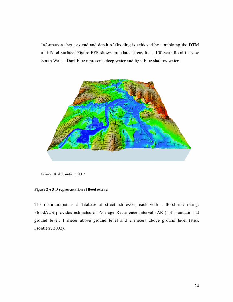
Information about extend and depth of flooding is achieved by combining the DTM
and flood surface. Figure FFF shows inundated areas for a 100-year flood in New
South Wales. Dark blue represents deep water and light blue shallow water.
Source: Risk Frontiers, 2002
Figure 2-6 3-D representation of flood extend
The main output is a database of street addresses, each with a flood risk rating.
FloodAUS provides estimates of Average Recurrence Interval (ARI) of inundation at
ground level, 1 meter above ground level and 2 meters above ground level (Risk
Frontiers, 2002).

25
2.4. Evaluation
In the section above flood risk assessment methods and models in different countries
were investigated. It was observed that these methodologies vary largely in different
countries. For example determination of infrastructure damages is covered in detail in the
“Multi-Coloured Manual” in United Kingdom but in Australia infrastructure damage
assessment seems to be limited while in United States it is not covered at all. In other
terms in these countries depth-damage curves for rural areas are not considered.
Components covered in different methodologies where tabulated in Table 2.6.
Table 2-6Coverage of existing flood loss estimation models
Damage Categories United States United Kingdom Australia Residential detail detail detail Urban Damage
Non-residential detail detail detail Crop damage rough rough rough
Farmland detail detail none Rural Damage
Fishery none detail detail System damage none detail rough Infrastructure
Service loss none detail rough Business Loss detail detail detail
Environmental Damage none detail none
When risk estimation models were observed it was noted that all models use unit loss
model. In other words they calculate the possible damage on a property-by-property
basis. Risk is calculated in all models by finding the possible damage for different flood
magnitudes and then weighting them with occurrence probability of respective floods.
Possible damages were found either by using absolute depth-damage curves or using
relative depth-damage curves and multiplying the damage percentages with the value of
assets.
26
It was also observed that all of the damage models were mainly developed for urban
damages. Rural damage functions were not considered in so much detail. In cases where
crop damage was considered, damage functions did not consider effects of high
groundwater levels. In other words depth-damage functions were plotted starting from
ground level. But in real life effects of high groundwater levels on crop damage are
known and must not be neglected.
All above mentioned models were developed for river and sea floods. Calculation of risk
for these kinds of floods differs from calculation of risk for floods occurring due to
precipitation exceeding drainage capacity. While assessing risk for sea and river floods,
structures are assigned a failure probability and risk is calculated as the product of this
probability and possible damage that will be caused if the structure fails. In floods due to
precipitation exceeding drainage capacity failure is not limited with one structure and
failure probability is not constant. Failure might occur frequently with small damage and
with a high damage but with lower frequency. Thus flood damage must be calculated
over Probability-Density function. Also probability depends on elevation of each pixel
and it is spatially distributed.
Above mentioned models are not capable of assessing risk when both probability and
possible damage are spatially distributed.

27
2.5. Conclusion
Common practices in flood risk assessment in different countries and different flood risk
models were investigated in order to find if any of these existent models are applicable to
the problem of assessment of flood damage due to precipitation exceeding drainage
capacity. The following conclusions were drawn.
1- All of the models studied were developed for floods caused by breaches of dunes
and levees and were not able to calculate risk for floods caused by precipitation
exceeding drainage capacity due to flowing reasons.
- These models calculate damage for several inundation maps with known
probabilities. But such a match of probability and inundation map for rainfall
induced floods in low lands is not possible.
- For this kind of floods failure is not limited to one section. Meaning, failure
probability differs from frequent floods with small damages to low frequency
floods with higher damage.
- Probability is also dependent on the elevation of the pixel. As a result probability
will be spatially distributed. Current models are not capable of calculating risk for
spatially distributed probability functions.
- Existing models do not cover effects of high ground water levels.
28
2- A new model must be developed that will be capable of handling the calculations
due to the spatially distributed nature of probability and damage data. A GIS
based model would be appropriate for this case. Probability and damage functions
can be modeled by two separate grid layers. This way risk can be calculated by
unit loss approach in terms of grid-by-grid consideration of risk.
3- Effects of high groundwater levels must be included in damage functions. As
current models were developed mostly for urban damage, these effects were
ignored. But for this kind of floods rural damage has a higher importance and
effects of high groundwater levels can not be ignored.

29
3. Correlation of flood depth and duration for different soil types
3.1. Introduction
As mentioned earlier, risk calculation for floods due to rainfall exceeding drainage
capacity differs from river and sea floods. In the second one failure probability is
constant but in the first case failure might occur frequently with small damage or less
frequently but with a higher damage. As a result of this risk must be calculated for all the
points on the probability distribution function of water levels. This means an enormous
work load for calculation of risk. Thus any simplifications that will decrease this work
load have great importance for such a risk model to work efficiently.
Most important parameters for damage calculations in risk models are flood depth and
flood duration. If these parameters can be replaced by one parameter the work load will
reduce significantly making it possible to calculate the risk.
In this chapter, correlation between flood depth and duration will be proved. As a result
of this correlation flood depth can be used solely, while effect of duration will be covered
inclusively. Relation between these parameters is dependent on drainage properties of the
soil. In order to include effects of soil properties, 12 soil types were investigated.
30
3.2. Methodology
Flood depth can be used as an indicative parameter. This is an acceptable assumption
since flood duration is closely related to flood depth. In other words, if the flood depth is
high then it will take more time to drain the flood plain, thus flood duration will be
longer. At this section of the study validity of this assumption was investigated.
In order to verify this assumption groundwater levels were simulated for a long enough
time period that would enable the researcher to comment statistically on the results.
These simulations were carried out with SOBEK Rainfall – Runoff Module for 12 most
common soil types in Netherlands. Results were investigated statistically in means of R-
Square and coefficient of correlation.
31
3.3. Model Schematization
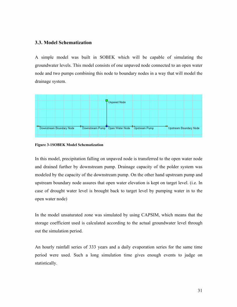
A simple model was built in SOBEK which will be capable of simulating the
groundwater levels. This model consists of one unpaved node connected to an open water
node and two pumps combining this node to boundary nodes in a way that will model the
drainage system.
Figure 3-1SOBEK Model Schematization
In this model, precipitation falling on unpaved node is transferred to the open water node
and drained further by downstream pump. Drainage capacity of the polder system was
modeled by the capacity of the downstream pump. On the other hand upstream pump and
upstream boundary node assures that open water elevation is kept on target level. (i.e. In
case of drought water level is brought back to target level by pumping water in to the
open water node)
In the model unsaturated zone was simulated by using CAPSIM, which means that the
storage coefficient used is calculated according to the actual groundwater level through
out the simulation period.
An hourly rainfall series of 333 years and a daily evaporation series for the same time
period were used. Such a long simulation time gives enough events to judge on
statistically.
32
3.4. Model Data
While setting up the model attention was given to input data in a way that the model will
be able to reflect the real world situation in the best way possible. In order to achieve this,
input data was determined by using previous studies, values used in common practice and
expert advice. In this part, input data used in the simulations were given for every node.
3.3.1. Unpaved Node:
An unpaved node of 100 ha was used as a representative land. Vegetation was chosen as
grass in order to avoid interference of vegetation in groundwater calculations. Parameters
used are explained in detail below and listed in TABLE 3.1.
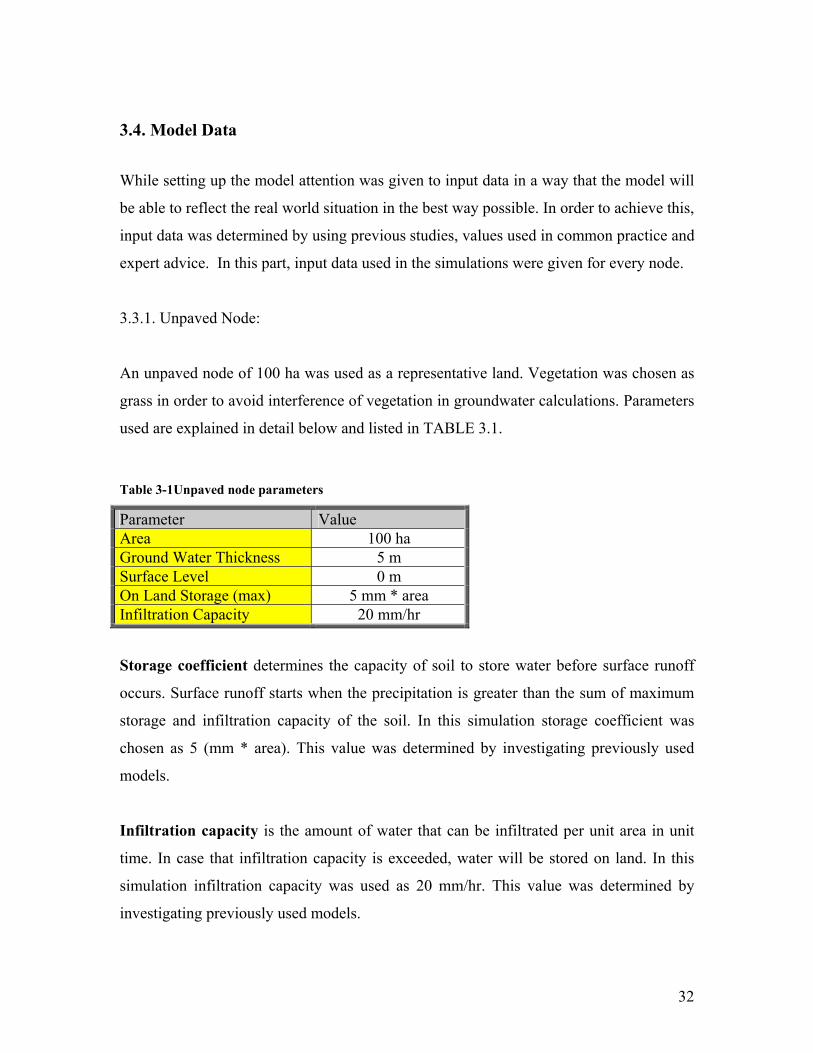
Table 3-1Unpaved node parameters
Parameter Value Area 100 ha Ground Water Thickness 5 m Surface Level 0 m On Land Storage (max) 5 mm * area Infiltration Capacity 20 mm/hr
Storage coefficient determines the capacity of soil to store water before surface runoff
occurs. Surface runoff starts when the precipitation is greater than the sum of maximum
storage and infiltration capacity of the soil. In this simulation storage coefficient was
chosen as 5 (mm * area). This value was determined by investigating previously used
models.
Infiltration capacity is the amount of water that can be infiltrated per unit area in unit
time. In case that infiltration capacity is exceeded, water will be stored on land. In this
simulation infiltration capacity was used as 20 mm/hr. This value was determined by
investigating previously used models.
33
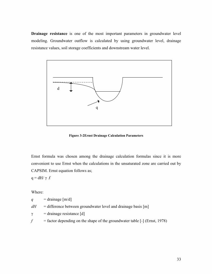
Drainage resistance is one of the most important parameters in groundwater level
modeling. Groundwater outflow is calculated by using groundwater level, drainage
resistance values, soil storage coefficients and downstream water level.
Figure 3-2Ernst Drainage Calculation Parameters
Ernst formula was chosen among the drainage calculation formulas since it is more
convenient to use Ernst when the calculations in the unsaturated zone are carried out by
CAPSIM. Ernst equation follows as;
q = dH/ γ .f
Where:
q = drainage [m/d]
dH = difference between groundwater level and drainage basis [m]
γ = drainage resistance [d]
f = factor depending on the shape of the groundwater table [-] (Ernst, 1978)
q
d
34
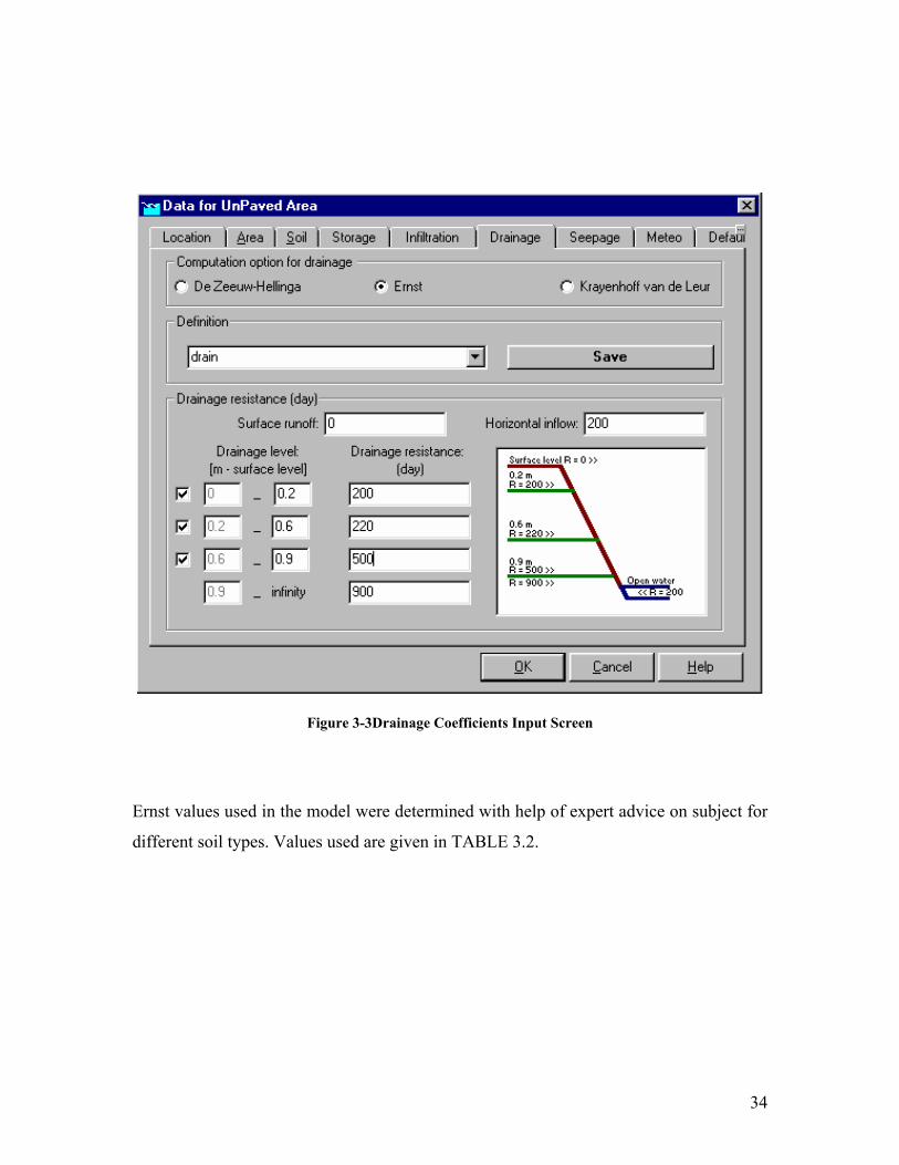
Figure 3-3Drainage Coefficients Input Screen
Ernst values used in the model were determined with help of expert advice on subject for
different soil types. Values used are given in TABLE 3.2.

35
Table 3-2Ernst coefficients for different soil types
Soil Type Ernst Coefficient Sand Maximum 50 Peat Maximum 10 Clay Maximum 20 Peat Average 20 Sand Average 20 Silt Maximum 50 Peat Minimum 10 Clay Average 20
Sand Minimum 50 Silt Average 20
Clay Minimum 20 Silt Minimum 50
3.3.2. Open Water Node:
A constant area of 5 ha was used as open water node. This area was again determined
according to regulations and previously carried out studies. Bottom level was determined
as “datum – 2m”. In this case bottom level does not have any importance because the
upstream pump will avoid an extensive decrease in the open water level by pumping in
water from the upstream boundary node. Target level of the open water node was set to
“datum – 1m”.
3.3.3. Pumps:
Upstream pump station functions in a way that will keep the open water level at target
value at times when rainfall is not encountered for a long period. This reflects the real
world situation, since in periods with out rainfall, decrease of groundwater level in
agricultural areas are prevented by controlling the open water level in the area by
pumping in water. On the other hand it does not have a direct impact on the aim of this
study. The study aims to model the drainage properties of soils under floods. If the
36
groundwater level is brought back to target level in case of drought, this will only
increase the number of events during the simulation period, which will make the results
statistically sounder. The upstream pump works as an inlet and checks downstream water
levels for operation.
Downstream pump station models the drainage system. It functions as a normal pump
and checks upstream water levels. If the target value is exceed it starts operating. In order
to avoid any lag, operation rules of the pump was set in a way that it would start
operation if the deviation from target level is 1cm. This is not the case in real world
operations due to the fact that such a management will increase operation costs. But since
the aim is modeling of the soil, this is an acceptable application in the model.
Pump capacity used in the model was 6.94m2/min. This value was determined as the
mean value of pumps that were used in previous studies.
3.3.4. Boundary nodes:
Boundary nodes were set in order to isolate the model. In other words with the help of
boundary nodes it was made sure that there will always be enough water in the upstream
to be used in case of drought and the downstream pump will always be able to pump out
the maximum capacity of the pump.

37
3.5. Post processing of simulation results
The aim of this study was obtaining a series of flood depth and flood duration parameters
and observing them statistically in order to prove the correlation between these
parameters. In order to obtain these series following processes were carried out.
In order to begin analysis parameters had to be defined first. Definitions used were as
follows. An event was defined as water level exceeding a given threshold. In this study
the threshold was defined as “datum - .70m”, in other words 30cm above the target level.
Flood duration was defined as the time between the first time that the water level
exceeds the threshold and the time when the water level goes below the threshold. Two
parameters were defined for flood depth, namely as “average depth” and “maximum
depth”. Maximum depth was defined as the flood depth at the time when the water level
reaches its highest value within an event while average depth was defined as the mean
value of flood depth through out the entire event duration.
Once the model was run, results were recorded to a history (.his) file. This history file
included hourly values of unpaved node parameters for 333 years. Since the simulation
period was excessively large, it was not possible to work further on these history files due
to large file sizes up to 1.5 gigabyte.
In order to be able to process, groundwater depth data were exported to tab separated text
(.txt) files. These files were containing water level values for almost 3 million time steps.
A script was written in visual basic in order to pick events within this large text file. The
script used hourly water levels as input and recorded another text file which involves
event duration, maximum depth and average depth parameters for every single event and
a summary of entire simulation period at the end of the file. (I.e. Number of events, total
duration above threshold, total simulation period) The script used is given in figure 3.4
and an exemplary output file view is given in figure 3.5.

38
Figure 3-4Visual Basic script for determination of events

39
Figure 3-5Output file view of the script
Results in this file were plotted as two series, namely as maximum and average. Series
“Maximum” indicates the duration and corresponding maximum groundwater level for
each event. While series “Average” indicates the duration of the event and the mean
value of groundwater level within that event.
Further on statistical operations were carried out on these data sets in order to observe the
correlation between these two parameters. First a trend line was calculated for each
series. In order to be able to observe the correlation coefficient, trend line was chosen to
be linear, which can be represented by the equation: y = (m*x) + b, and can be calculated
by least squares fit method. Then coefficient of determination (i.e. R square) and
correlation coefficient was calculated for each series.

40
Coefficient of determination (R2) is the proportion of a sample variance of a response
variable that is "explained" by the predictor variables when a linear regression is done. In
other words it is the proportion of the variability in one series, it is a measure of the
quality of fit. 100% R-square means perfect predictability.
The formula for R2 is
where,
ESS = explained sum of squares,
RSS = residual sum of squares, and
TSS = total sum of squares.
Correlation coefficient (r), indicates the strength and direction of a linear relationship
between two random variables. In general statistical usage, correlation refers to the
departure of two variables from independence. The correlation coefficient will vary from
-1.0 to 1.0. -1.0 indicates perfect negative correlation, and 1.0 indicates perfect positive
correlation.
If there is only one predictor variable than correlation coefficient can be calculated as the
square root of coefficient of determination.
2Rr =

41
3.6. Results
Above mentioned operations were carried out for 12 different soil types. After the post
process of simulations flood depth – flood duration graphs were plotted. Examples of
these graphs for average and maximum values can ve observed in figure 3.6 and figure
3.7 respectively.
Sand Average - Average
y = 0.0009x - 0.6829R2 = 0.8016
-0.8
-0.7
-0.6
-0.5
-0.4
-0.3
-0.2
-0.1
00 50 100 150 200 250 300
Duration (h)
Dep
th (m
)
AverageLinear (Average)
Figure 3-6Depth – Duration graph for Sand Average (average)

42
Sand Average - Maximum
y = 0.0041x - 0.6816R2 = 0.7691
-0.8
-0.6
-0.4
-0.2
0
0.2
0.4
0.6
0 50 100 150 200 250 300
Duration (h)
Dep
th (m
)
MaximumLinear (Maximum)
Figure 3-7Depth – Duration graph for Sand Average (maximum)
Linear trend lines were calculated by least square fit method for each soil type. Trend
lines for average and maximum flood height values for different soil types are shown in
Figure 3.8 and Figure 3.9.

43
Depth - Duration Average
Sand Maximum
Peat Minimum
Peat Maximum
Clay Maximum
Peat Average
Sand Average
Silt Maximum
Clay Average
Sand Minimum
Silt Average
Clay Minimum
Silt Minimum
-0.8
-0.6
-0.4
-0.2
0
0.2
0.4
0.6
0 100 200 300 400 500 600
Duration (h)
Dep
th (m
)
Figure 3-8Trend lines of different soil types (average)
Depth - Duration Maximum
Sand Maximum
Peat Maximum
Clay MaximumPeat Average
Silt Maximum
Peat Minimum
Sand Average
Clay Average
Sand Minimum
Silt Average
Clay Minimum
Silt Minimum
-1
-0.5
0
0.5
1
1.5
2
2.5
3
0 100 200 300 400 500 600
Duration (h)
Dep
th (m
)
Figure 3-9Trend lines of different soil types (maximum)

44
Then coefficient of determination was determined for every different soil type. Resulting
R-square values are given in the table 3.3 for average and maximum flood depth cases.
Table 3-3Coefficient of Determination for different soil types
Soil Type R^2 (Average) R^2 (Maximum) Peat Minimum 0.359 0.425 Silt Average 0.361 0.377 Clay Minimum 0.450 0.431 Clay Average 0.482 0.441 Clay Maximum 0.571 0.495 Peat Average 0.623 0.522 Silt Maximum 0.707 0.686 Sand Maximum 0.724 0.704 Silt Minimum 0.724 0.706 Sand Minimum 0.735 0.718 Peat Maximum 0.748 0.692 Sand Average 0.802 0.769
Correlation coefficient was calculated as square root of coefficient of determination.
Resulting r values are given in the table 3.4.
Table 3-4Correlation Coefficient for different soil types
Soil Type Correlation Coefficient (Average)
Correlation Coefficient (Maximum)
Peat Minimum 0.60 0.65 Silt Average 0.60 0.61 Clay Minimum 0.67 0.66 Clay Average 0.69 0.66 Clay Maximum 0.76 0.70 Peat Average 0.79 0.72 Silt Maximum 0.84 0.83 Sand Maximum 0.85 0.84 Silt Minimum 0.85 0.84 Sand Minimum 0.86 0.85 Peat Maximum 0.86 0.83 Sand Average 0.90 0.88
45
3.7. Evaluation & Conclusion
In this section drainage characteristics of 12 most common soil types in Netherlands were
simulated. Main aim of this simulation was to see the correlation between flood depth
and flood duration. Following conclusions were drawn from the simulations.
1- Correlation between flood depth and flood duration was proved. Thus it will be an
acceptable assumption to disregard flood duration and use flood depth as an
indicative parameter which will cover both coefficients. This will decrease the
computational workload significantly.
Correlation coefficient was noted to have an average of 0.77. The lowest value
was 0.60 for peat minimum and silt average, while the highest value reaches to
0.90 for sand average. This value represents a strong positive correlation between
flood depth and flood duration.
2- Trend lines for depth – duration relation was created from simulation results. It
was observed that trendlines for clay was steeper than the ones for sand. This was
an expected result due to the differences in permeability and storage coefficient.
Flood depth tends to increase faster, reaches higher values, and remains high for a
longer period in clay. While in sand, increse in flood depth is rather slowly and
drainage is faster compared to clay. This explains the differences in slopes of
trend lines.
3- Coefficient of determination was noted to decrease with increasing trend line
slope. This is due to two main reasons. A lower trend line slope means faster and
rather simple drainage. But in a steeper trend line, drainage is rather slow and
other parameters like horizontal flow or effects of consequent rainfall events
make it harder to be modeled linearly. Second reason is statistical. With the
increasing slope of trend line number of events will increase. Thus with more
events, number of deviations from the trend line also increases.
46
4. Case Study: Polder Berkel
4.1. Introduction
A case study was carried out in order to investigate the applicability of a new risk
analysis tool to floods due to precipitation exceeding drainage capacity. For this purpose
the risk analysis tool that works on GIS basis using land use data, digital elevation model
and probability density function of water levels was used to calculate the risk in the case
study area.
The risk calculated by the above mentioned risk analysis tool was compared with risk
calculated by the risk calculated by another method namely as WB21. (Abbreviation for
Waterbeheer 21st) As a matter of fact WB21 is not a risk model. It is rather a method for
damage calculation for single events. But a risk value was obtained by summing up
damage for every single event in a long enough period and dividing this damage sum to
the simulation period.
It must be noted that this case study does not aim to show the correlation between flood
depth and duration which was proved in previous chapter since there exist many other
parameters that effect the calculations within each model. But it must be also noted that
the risk analysis tool used calculates the risk according to the fact that these two
parameters are correlated.
Further detail on both models will be given below. This chapter starts with brief
introduction about the study area: Polder Berkel, follows with descriptions of both
methods, comparison of results obtained and concludes with comparison and discussion
of case study outcomes.
47
4.2. Polder Berkel The case study was carried out in Polder Berkel. The main reason for selecting this area
as the case study area was the accessibility of meteorological data and rainfall-runoff
model. In this section general information about the case study area will be provided.
Polder Berkel lies between Rotterdam and Zoetermeer and covers an area of 2.052 ha. It
lies within the borders of Berkel and Rodenrijs and Pijnacker-Nootdorp municipalities.
The polder is divided into 12 sub-polders with 7 different target levels. The area is
drained by three main drains to Binnenboezem. Sub-polders within the polder are named
as follows,
1. Bergboezem
2. Meerpolder
3. Nieuwe droogmaking
4. Nieuwe Rodenrijsche droogmakerij
5. Noordpolder
6. Oostmeerpolder
7. Oudeland
8. Oude Leede
9. Voorafsche polder
10. Westpolder
11. Zuidpolder
12. Zuidpolder Rodenrijs
Water level within the polder varies from -1.5m + NAP (abbreviation for Normaal
Amsterdams Peil, i.e. Normal Amsterdam Water Level) in the middle parts of the
Oudeland and -5.85m + NAP in the Zuidpolder. Sub-polders Oudeland and Voorafsche
Polder are relatively higher within the main polder with an average level of -2.7m +
NAP. On the other hand the Bergboezem, Westpolder and Zuidpolder are the lowest
areas in the case area with an average elevation of -5.1m +NAP. A general view of the
sub-polders and target elevations for summer and winter season is given in Figure 4.1.

48
Source: TAUW, 2002
Figure 4-1Sub-polders and target elevations

49
Prevailing soil type in the polder is clay. The polder is mostly covered with grass and
agriculture. Percentage of grass and agricultural areas reaches to 64% while green houses
cover 14% of the total area. 14% of the polder is used as urban. This distribution can be
observed from the satellite image in Figure 4.2.
Figure 4-2Satellite Image of Polder Berkel
50
4.3. WB21 Method This method had been presented for modeling damage due to high groundwater levels.
Main reason of this damage is the fact that high ground water levels cause anaerobic
conditions in the root zone and this leads to drowning of the crop. Other effects of high
groundwater level on crop productivity are as follows:
- Growing season for crops is shortened due to decreased yield and low temperature.
- Fine soil particles form a crust layer.
- Due to denitrification, nutrients that feed the crops are lost.
- With high groundwater brackish or salt water can reach to root zone.
The proposed model uses the general formula given below for damage calculations.
max*),( DthfD ∆=
Where;
D = damage per hectare
),( thf ∆ = damage function dependent of depth and duration
maxD = maximum damage
Damage functions and maximum damage amounts are depended on land use. This
method uses 5 different land use form. Maximum damage amounts for different land use
forms are given in Table 4.1. These amounts were calculated by Agriculture Economic
Institute (Landbouw Economisch Instituut, LEI) as the average gross real turnover by
hectare.
51
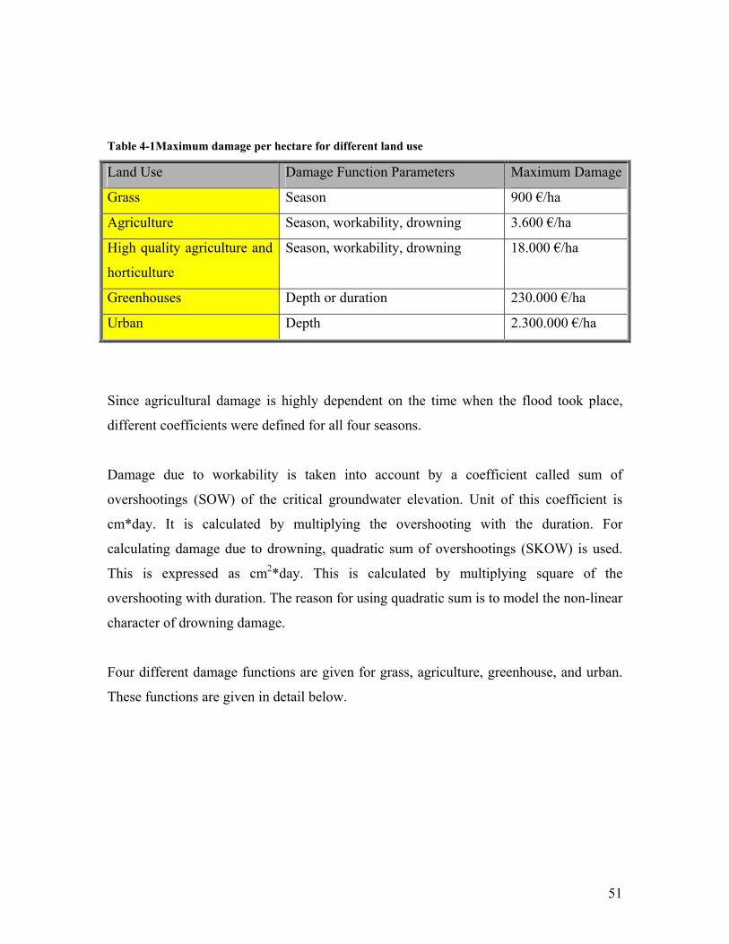
Table 4-1Maximum damage per hectare for different land use
Land Use Damage Function Parameters Maximum Damage
Grass Season 900 €/ha
Agriculture Season, workability, drowning 3.600 €/ha
High quality agriculture and
horticulture
Season, workability, drowning 18.000 €/ha
Greenhouses Depth or duration 230.000 €/ha
Urban Depth 2.300.000 €/ha
Since agricultural damage is highly dependent on the time when the flood took place,
different coefficients were defined for all four seasons.
Damage due to workability is taken into account by a coefficient called sum of
overshootings (SOW) of the critical groundwater elevation. Unit of this coefficient is
cm*day. It is calculated by multiplying the overshooting with the duration. For
calculating damage due to drowning, quadratic sum of overshootings (SKOW) is used.
This is expressed as cm2*day. This is calculated by multiplying square of the
overshooting with duration. The reason for using quadratic sum is to model the non-linear
character of drowning damage.
Four different damage functions are given for grass, agriculture, greenhouse, and urban.
These functions are given in detail below.

52
4.3.1. Grass Damage
Damage in grass land is mainly due to workability condition thus it is dependent on soil
type and season. In this method, this differentiation is made by a coefficient called
workability coefficient for grass land. Values of this coefficient are given in Table 4.2.
Damage function for grass land is given as follows.
cdSOWtcthf *)(),( 0=∆
Where;
)(0 tc = workability coefficient for grass land (cm-1*d-1)
cdSOW = sum of overshootings for given critical depth (cm*d)
Table 4-2Workability coefficients for seasons and soil types for grassland
Season (cm-1*d-1) (cm-1*d-1) (cm-1*d-1)
Spring 20*10-5 10*10-5 5*10-5
Summer 26*10-5 17*10-5 17*10-5
Autumn 6*10-5 8*10-5 8*10-5
Winter 0 0 0
Critical Depth (cm) 20 40 75
4.3.2. Agriculture and Horticulture Damage
Damage on agriculture is mostly dependent on the drowning of plants. Damage function
is defined in a way that water level exceeding the root zone for three days causes
complete loss of the crop. (Bolt et.al., 2000). Further on damage function is defined as the
maximum of the damage due to workability and damage due to drowning. And it must be
kept in mind that it can not be greater then 1 since damage function equal to 1 means
100% damage and a higher damage is not possible.
53
)*)(,*)(max(),( 21 rzcd SKOWtcSOWtcthf =∆
Where;
)(1 tc = workability coefficient (cm-1*d-1)
cdSOW = sum of overshootings for given critical depth (cm*d)
)(2 tc = drowning coefficient (cm-2*d-1)
rzSKOW = sum of overshootings for given root zone (cm2*d)
Coefficients to be used in the above formula are given in tables below. Differentiation for
this coefficient was made with respect to seasons and soil types. Table 4.3 gives the
workability coefficient for agriculture. Workability coefficient for high quality
agriculture and horticulture is given in Table 4.4 and drowning coefficients are given in
Table 4.5.
Table 4-3Workability coefficients for seasons and soil types for agriculture
Season Sand (cm-
1*d-1)
(cm-1*d-1) (cm-1*d-1) (cm-1*d-1) (cm-1*d-1)
Spring 8*10-5 9*10-5 8*10-5 9*10-5 10*10-5
Summer 14*10-5 15*10-5 14*10-5 16*10-5 16*10-5
Autumn 7*10-5 7*10-5 7*10-5 8*10-5 8*10-5
Winter 0 0 0 0 0
Critical Depth (cm) 85 120 150 120 140

54
Table 4-4Workability coefficients for high quality agriculture and horticulture
Season Sand (cm-
1*d-1)
(cm-1*d-1) (cm-1*d-1) (cm-1*d-1) (cm-1*d-1)
Spring 14*10-5 14*10-5 14*10-5 16*10-5 16*10-5
Summer 24*10-5 24*10-5 23*10-5 27*10-5 27*10-5
Autumn 11*10-5 12*10-5 11*10-5 13*10-5 13*10-5
Winter 0 0 0 0 0
Critical Depth (cm) 85 120 150 120 140
Table 4-5Drowning coefficients
Season (cm-2*d-1) (cm-2*d-1) (cm-2*d-1) (cm-2*d-1) (cm-2*d-1)
Spring, Summer,
Autumn
21*10-5 21*10-5 21*10-5 7*10-5 5*10-5
Winter 0 0 0 0 0
Root Zone Depth 40 40 40 70 80
4.3.3. Greenhouses Damage
In greenhouses high groundwater levels do not causes damage. In this case damage is
caused by inundation. Two different damage functions were defined for greenhouses.
First function is dependent on inundation depth while the second one is dependent on
inundation duration. Damage functions for greenhouses are as follows.
)1,*6.12.0min()( hhf +=
)1,*06.05.0min()( 2ttf ∆+=∆
Where;
h = inundation depth (m)
t∆ = inundation duration (d)

55
4.3.4. Urban Damage
In this method urban damage is modeled according to the depth damage function given
below. (See Figure 4.3)
)1,01.0min()( hhf +=
Where;
h = inundation depth (m)
Damage Functions
0
10
20
30
40
50
60
70
80
90
100
-0.2 0 0.2 0.4 0.6 0.8 1 1.2 1.4 1.6
Inundation depth (m)
Dam
age
perc
enta
ge (%
)
UrbanGreenhouses
Figure 4-3Damage Function for Greenhouses and Urban Areas
4.3.5. Simulation and Risk Calculation
For calculation of risk water levels within the polder had to be simulated for both
methods. This simulation was carried out in SOBEK Rainfall-Runoff module. Model
used for this simulation can be seen in Figure 4.4.

56
Figure 4-4SOBEK Model for Polder Berkel
This simulation was run for 100 year long time period and groundwater and open water
elevations were recorded for this period. Since the file size of these records were
extensively large, these files were converted to tab separated text files, making it possible
to further process this data.
As it was mentioned earlier WB21 method is capable of calculating damage per event. In
order to be able to calculate a risk value with this method, damage caused by all events
within a period had to be calculated one by one and the yearly average of these damages
would be the annual average risk value calculated with this method. Time period must be
chosen long enough that this definition of annual average risk will be valid. In this study
a 100-years period was chosen.
57
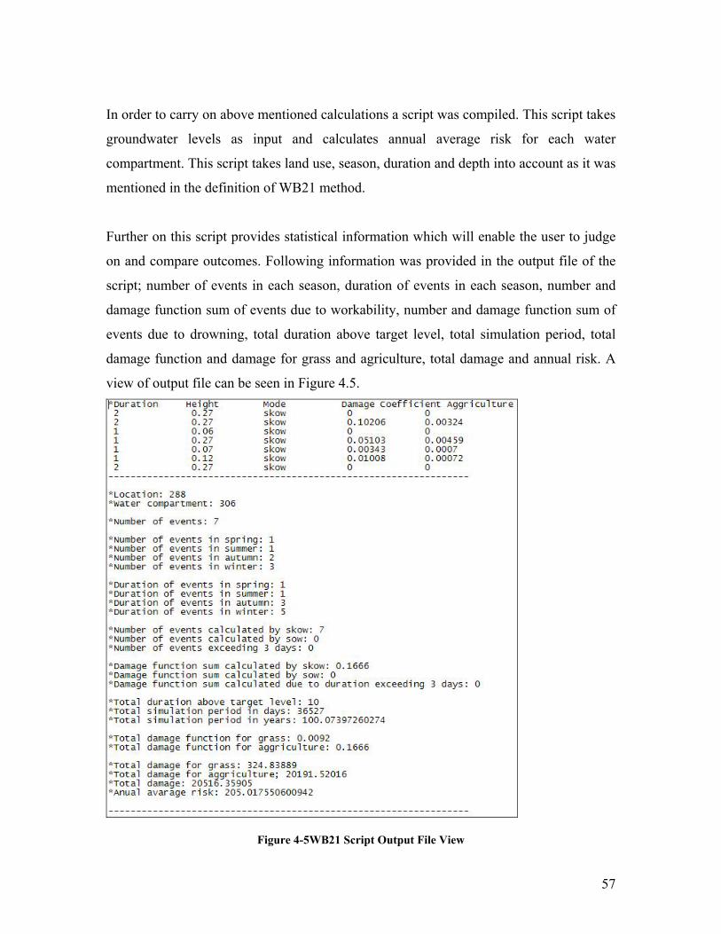
In order to carry on above mentioned calculations a script was compiled. This script takes
groundwater levels as input and calculates annual average risk for each water
compartment. This script takes land use, season, duration and depth into account as it was
mentioned in the definition of WB21 method.
Further on this script provides statistical information which will enable the user to judge
on and compare outcomes. Following information was provided in the output file of the
script; number of events in each season, duration of events in each season, number and
damage function sum of events due to workability, number and damage function sum of
events due to drowning, total duration above target level, total simulation period, total
damage function and damage for grass and agriculture, total damage and annual risk. A
view of output file can be seen in Figure 4.5.
Figure 4-5WB21 Script Output File View

58
4.4. Risk Model
The second model used in this study was a GIS based risk model. This model takes
various data as input and calculates the annual average risk accordingly. Input files for
this model can be categorized into two as, GIS data and other data.
- GIS Data (maps in asci file format)
- Digital Elevation Map (DEM)
- Water compartments
- Land use map
- Other Input Data (data in comma separated value (csv) file format)
- Target levels for water compartments
- Damage functions and maximum damage values
- Probability density functions for open water levels
In order to run this model a digital elevation map of 25m X 25m was used. This map can
be seen in Figure 4.6.
In order to assess damage for sub-polders with different target elevations, water
compartments were defined. These compartments were defined according to the unpaved
nodes in the SOBEK model. A detailed presentation of these water compartments can be
observed in Figure 4.7.

59
Figure 4-6Digital Elevation Map Figure 4-7Water Compartments
Land use data was provided by a 25m X 25m land use file which consists of 16 major
land use types. This land use map can be seen in Figure 4.8.
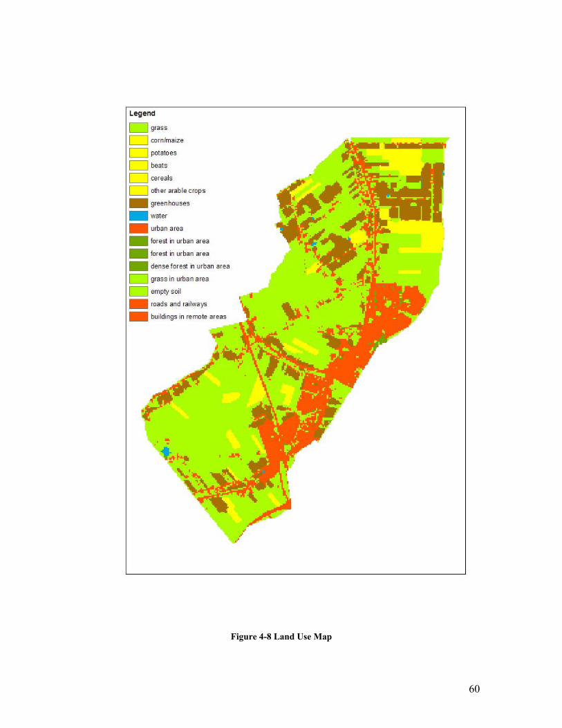
60
Figure 4-8 Land Use Map

61
Target level values for each compartment were defined in a csv file. Target values were
calculated in a way that results from two methods will be comparable. In order to achieve
this, target levels were set for every water compartment to mean elevation of the water
compartment minus root zone depth.
Maximum damage values and damage functions for different land use types were entered
in another csv file. Damage functions used in this study can be observed from Figure 4.9.
(Hoes, 2005)
Damage Functions
0
10
20
30
40
50
60
70
80
90
100
-50 -40 -30 -20 -10 0 10 20 30 40
Inundation depth (cm)
Dam
age
perc
enta
ge (%
)
CropsGrassUrban
Figure 4-9Risk Model Damage Functions
Final input file used for this model was the file containing probability-density functions
for each water compartment. These functions were calculated by using a statistical
analysis program namely, Hymstat by considering 100 year long open water simulation
results. Hymstat output graph can be observed in Figure 4.10.

62
Gumbel Distribution Location: 402
Gumbel Distribution B = 0.04 X0 = -5.35
regression line reduced variate observed frequencies low er confidence limit dataupper confidence limit data
Frequencies0.1 0.2 0.5 0.8 0.9 0.95 0.99 0.999 1- - - - - - - - - - - - - - - - - - - - - - - - - - - - - - - -
Return Period1.111 2 5 10 20 100 1,000 10,000
redu
ced
varia
te o
bser
ved
frequ
enci
es
-5
-5.05
-5.1
-5.15
-5.2
-5.25
-5.3
-5.35
-5.4
-5.45
Figure 4-10Hymstat Output
Risk model creates two out files. First one is a csv file containing damage values for each
water compartment. The second output is a risk map in the form of an Asci file. This file
was converted to raster by using Arc Catalog. The raster form provides more user
friendly visualization of the risk values. Resulting risk map can be observed in Figure
4.11.
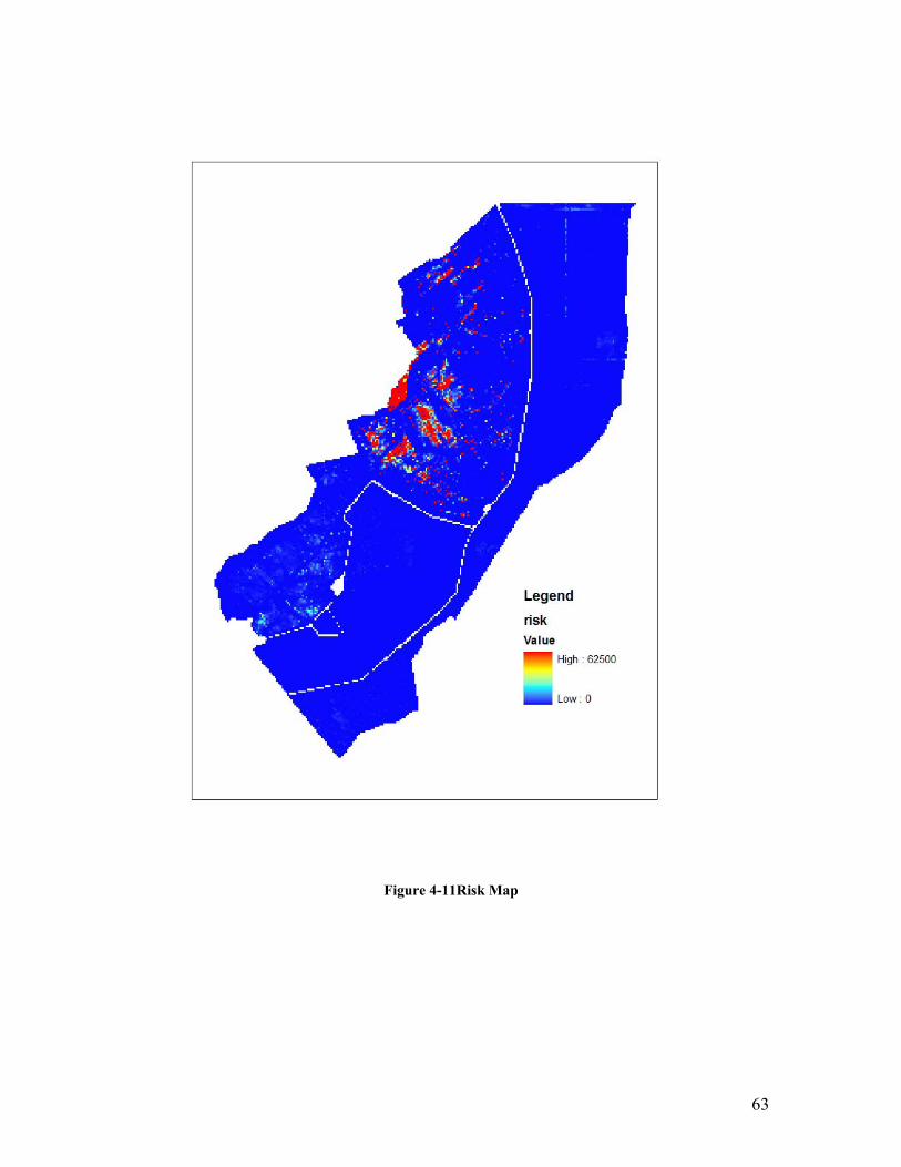
63
Figure 4-11Risk Map
64
4.5. Case Discussion & Comparison
Two models were run separately and resulting annual average risk values were compared.
Annual average risk calculated by the risk model was 32055 € while the one calculated
by the WB21 method was 33268 €. These two values represent almost a perfect match.
The difference in between these numbers is 3.6%.
When the results for each water compartment were investigated separately, it was noted
that the perfect match mentioned above was not the case. It was rather a coincidence.
Differences between risk values were observed in some of the water compartments. Risk
values of all water compartments calculated by both methods can be observed in Table
4.6.

65
Table 4-6Risk calculated by Risk Model and WB21 method
Risk in € calculated by Water Compartment Number Risk Model WB21 Method
306 200 205312 81 33317 5 0322 146 7325 1 0330 7 0336 0 0337 5 0344 54 6178346 0 0352 2 594359 0 8364 5 692367 0 0373 18 84377 22 997383 190 81385 1031 5793389 2719 173395 357 109399 1309 2800402 13 77407 4275 3667411 11353 7972414 1785 280419 34 1018423 144 467427 179 104430 531 0434 7587 1930
Table 4.7 provides information about the extent of difference between two results. In this
table monetary difference and ratio between two models were given for every water
compartment.

66
Table 4-7Monetary Difference and Ratio between Risk Model and WB21 method
There exist many differences between the two methodologies used. Considering these
differences, it would not be reasonable to expect same results from both models. In the
remainder of this case study, water compartments with significantly different risk values
were investigated in order to find out the reasons of these distinct values. This
investigation was carried out on various grounds and some rationales behind these
differences were found. Investigated parameters were effects of season of occurrence of
events, elevation differences within water compartments and land use data in a water
compartment. These parameters will be mentioned in detail below.
Water Compartment Number
Monetary Difference (€) (RM – WB21)
Ratio (greater/smaller)
306 -5 1.03 312 49 2.49 317 5 --- 322 139 20.34 325 1 --- 330 7 --- 336 0 --- 337 5 --- 344 -6124 113.41 346 0 --- 352 -592 260.59 359 -8 --- 364 -686 131.24 367 0 --- 373 -67 4.77 377 -975 46.19 383 109 2.35 385 -4762 5.62 389 2546 15.68 395 248 3.28 399 -1490 2.14 402 -64 6.06 407 609 1.17 411 3382 1.42 414 1506 6.38 419 -984 29.81 423 -322 3.23 427 75 1.72 430 531 --- 434 5657 3.93

67
4.5.1. Season of occurrence of events,
Season of occurrence of events data was derived from the outcomes of the script for
WB21 method. It was observed that water compartments with more events occurring in
the winter season tend to give higher risk values for the Risk Model case.
The main reason behind this is the fact that WB21 considers occurring time of events and
damage function for events occurring in winter is predefined as zero. Thus no risk is
introduced due to these events. While in the risk model no distinction between events
occurring in winter and events occurring in growth season of crops was made. While
preparing water level probability functions for Risk Model winter water levels were also
considered. This leaded to higher probability of occurrence and thus higher risk.
4.5.2. Elevation differences within a water compartment
Elevation differences within the water compartments were investigated through the
digital elevation map. With proper geographical information systems operations
statistical data about the variation of elevation for every water compartment was
produced. This data included mean value, range and standard deviation.
It was observed that in compartments with higher standard deviation more distinct values
were observed. But in this case distinction was not systematic as it was in the previous
parameter. (ie. Effect of seasons were always in a way that will cause a higher risk in
Risk Model results, but variability of elevation might lead to higher or lower risk values)
Main difference is, in WB21 method a single elevation (ie. Mean elevation) was used for
the entire water compartment while in the risk model digital elevation model was used.
This led to real elevation data in the scale of 25 m by 25 m pixels. This might have an
increasing or decreasing effect on risk values.

68
Consider an event with a maximum groundwater level a little bit lower than the mean
value of the entire water compartment. In this case WB21 method will not give any
damage since the mean value is not exceeded and this is not considered as an event. But
on the other hand Risk Model will calculate damage for pixels that lie below that
groundwater level. This will lead the Risk Model to give higher results compared with
the WB21 method.
On the other hand when we consider an event with a groundwater level just above the
mean elevation level, WB21 method will react as if the entire water compartment is
flooded. But it is not the actual case. Areas above this groundwater level is not inundated,
thus does not introduce any damage. Risk Method takes this fact into account and does
not introduce any damage for the pixels that are above the groundwater level.
Two examples mentioned above show that an approach based on DEM will be more
accurate.
4.5.3. Land use
It was also observed that the difference was greater in compartments where the
percentage of agriculture and horticulture was higher. This difference is due to the fact
that maximum damage coefficients for agriculture and horticulture are greater than
grassland. Thus if the damage functions are different, difference in risk will be higher for
agriculture compared with grass land.

69
4.6. Conclusions
In this chapter, WB21 damage assessment method for single events were modeled in a
way that 100 year period can be simulated and an annual average risk can be obtained as
an outcome and a GIS based risk model was used to calculate the risk in the same area.
Results were compared leading to following conclusions.
1- The risk model can be used for calculation of risk for floods due to precipitation
exceeding drainage capacity with small modifications. Yet the risk value alone is
not sufficient to judge on effectiveness of different methods unless they are
modeled by exactly the same methodology since the results are affected largely by
the way the damage is modeled.
2- There exist differences between two results. When the rationale behind this
difference was further investigated, two main parameters were seen to be
significantly effective. These are;
- Occurrence season of events
- Variation in elevation within a water compartment.
3- Time of occurrence must be taken into account for more accurate results, as the
crop loss will be less in event occurring in winter compared with the events
occurring in growth season. It was noted that this factor was not considered in the
Risk Model used.
4- Variations in elevation within a polder are also effective on the resulting risk. If
this variation is not included in the risk model, deviations from the real risk will
occur in the results. This deviation is can be either in a way that will increase the
risk or in a way that will decrease the risk. It is not possible to predict its effect
before hand. Risk Model used overcomes this problem by including the real
elevation data in terms of digital elevation map and provides more accurate
results.
70
5. Conclusions & Recommendations
Due to climate change extreme precipitation events follow an increasing trend. Combined
with the land subsidence and sea level rise, this leads to an increase in the frequency of
rainfall induces regional floods in low lands. Also as a result of on going urbanization
land value increases. As a combination of all these reasons, risk of floods due to rainfall
exceeding drainage capacity gains importance.
This study was carried out for investigating the risk calculation for floods due to rainfall
exceeding drainage capacity. The research was in three folds, namely as research on
existing flood risk models in chapter two, investigation of correlation between flood
depth and flood duration parameters in chapter three and a case study in order to calculate
the risk of flooding due to rainfall exceeding drainage capacity. Conclusions and
recommendations concerning this study are as follows.
71
5.1. Conclusions
1- A new model must be developed since non of the existing models are capable of
calculating risk for floods caused by precipitation exceeding drainage capacity due to
flowing reasons.
- For this kind of floods failure is not limited to one section. Meaning, failure
probability differs from frequent floods with small damages to low frequency
floods with higher damage.
- For this kind of floods failure is not limited to one section. Meaning, failure
probability differs from frequent floods with small damages to low frequency
floods with higher damage.
- Probability is also dependent on the elevation of the pixel. As a result probability
will be spatially distributed. Current models are not capable of calculating risk for
spatially distributed probability functions.
- Existing models do not cover effects of high ground water levels.
2- Correlation between flood depth and flood duration was proved. This proof has great
importance for calculation of flood risk for floods due to precipitation exceeding
drainage capacity. Based on this correlation flood duration parameter can be
disregarded and flood depth can be used as an indicative parameter which will cover
both coefficients. This will decrease the computational workload significantly and
make the calculation of risk for this kind of floods possible.

72
3- Risk analysis tool described in chapter 4 can be used for calculation of risk due to
floods exceeding drainage capacity with small alterations. Comparisons showed that
occurrence season of the events is an important parameter in risk calculations and it
was not covered in the risk analysis tool. In order to acquire accurate results, this
parameter has to be included in calculations. This can be done by altering the
program in a way that seasonal duration density functions of water elevations will be
used.
4- The way of modeling the damage has a vast effect on the risk. Thus risk value alone
will not be sufficient for comparison of effectiveness of different measures unless the
exact same methodology is used for both calculations.

73
5.2. Recommendations
The risk of floods due to precipitation exceeding drainage capacity increased
considerably in last decades. And none of the currently used models are capable of
calculating this risk thus more studies must be carried on for development of such a
model and integration of this model to commercially available models.
It was proved that flood depth and flood duration are strongly correlated. This correlation
allows elimination of one of these parameters from flood damage calculations. This is an
important issue for rainfall induced regional floods’ risk derivation since it is calculation
demands high calculation load and this load can be decreased by using this assumption.
Comparisons of the Risk Model showed that elevation must be an integral part of risk
calculation for this kind of floods. Thus a GIS based model which includes digital
elevation map is necessary.
Comparisons also showed a shortcoming of the Risk Model. The risk model does not
include the effects of seasons in agricultural damage calculation. Especially it must be
considered that extreme events occur more frequently in winter season, when there are no
crops on the fields. Thus the damage introduced in winter must be significantly lower
than the ones occurring in the growth season of the crops.
This can be included in the Risk Model by creating seasonal frequency distribution
functions for water levels. This means that a different distribution function must be
prepared for every season and maximum damage coefficients must be determined for
different seasons. This will increase the accuracy of the calculated risk considerably.

74
Finally the depth – damage functions used in the model were rather simple damage
functions, which were build considering main rationales behind flood damage like root
zones or building heights. These depth–damage functions must be calibrated according to
flood data and functions for other land use types must be derived.

75
6. References Bruijn, K.M. de, Heijer, F. Den, 2001, Flood Damage Modeling in The Netherlands:
Preliminary Report Status Quo, Trend and Event Analysis, WL Delft Hydraulics,
Delft, The Netherlands
Bruijn K.M. de, 2005, Resilience and Flood Risk Management: A systems Approach
Applied to Lowland Rivers, Delft University Press
Burnham, M. W., Dotson, H. W., Overview of the Flood Damage Analysis Program
(HEC-FDA), 1997 October 20-22,1997; Pacific Grove, California. US Army Corps of
Engineers, Hydrologic Engineering Center p 137-153
Defra, Department for Environment Food and Rural Affairs, July 2003, Flood and
Coastal Erosion Risk Management Research News, Issue 4
Defra, Department for Environment Food and Rural Affairs, August 2004, Modelling and
Decision Support Framework (MDSF): History & Overview
Defra, Department for Environment Food and Rural Affairs, May 2004, Modelling and
Decision Support Framework (MDSF): Procedures Version 3.1
Dutta, D., Herath, S., Musiake, K., 2001, Direct Flood Damage Modeling Towards Urban
Flood Risk Management, International Center for Urban Safety Engineering
(ICUS/INCEDE), IIS, The University of Tokyo, Japan
Penning-Rowsell, E.C., Chatterton, J.B., Day, H.J., Ford, D.T., Greenaway, M.A., Smith,
D.I., Wood, T.R., Witts, R.C., 1987, Comparative Aspects of Computerized
Floodplain Data Management, Journal of Water Resources Planning and
Management, Vol.113, No.6
FEMA, Federal Emergency Management Agency, August 2004, Using HAZUS-MH for
Risk Assessment: How-To Guide
Hoes, Olivier, 2005, Risk Assessment to Quantify the Interaction Between Land Use and
Water Management, ERSA-Congress, Amsterdam, The Netherlands
IPCC, International Panel on Climate Change, 2001, Climate Change 2001: Impacts,
Adaptation and Vulnerability, Cambridge University Press

76
Jonkman, S.N., Brinkhuis-Jak, M., Kok, M., 2004, Cost Benefit Analysis and Flood
Damage Mitigation in the Netherlands, HERON, vol. 49, issue 1
Lekuthai, A., Vongvisessomjai, S., 2001, Intangible Flood Damage Quantification, Water
Resources Management, Vol. 15, No. 05 pp:343-362
NR&M, Queensland Government Natural Resources and Mines Department, 2002,
Guidance on the Assessment of Tangible Flood Damages
Penning-Rowsell, E. et al., 2003, The Benefits of Flood and Coastal Defence: Techniques
and Data for 2003, Flood Hazard Research Centre (FHRC), in press
Penning-Rowsell, E. et al., 2005, Guidelines for Socio-Economic Flood Damage
Evaluation: 1st Draft Version, FLOODsite
Risk Frontiers, 2002, Risk Frontiers Quarterly Newsletter, vol. 1, no. 4, July 2002
USACE, 1988, National Economic Development Procedures Manual: United States
Army Crops of Engineers, Fort Collins, USA
USACE, 1998, HEC-FDA Flood Damage Reduction Analysis: User’s Manual, United
States Army Crops of Engineers, USA

77
7. Appendix
List of appendix:
1. Flood depth – Flood duration graphs for 12 must common soil types 2. Frequency distribution graphs of water elevations for water compartments 3. Script designed for WB21 model 4. Output file of the WB21 script 5. Statistical information on elevation data of water compartments

78
1 - Flood depth – Flood duration graphs for 12 must common soil types
Sand Maximum - Average
y = 0.0006x - 0.6856R2 = 0.7237
-0.8
-0.7
-0.6
-0.5
-0.4
-0.3
-0.2
-0.1
00 100 200 300 400 500 600
Duration (h)
Dep
th (m
)
AverageLinear (Average)
k
Sand Maximum - Maximum
y = 0.0022x - 0.6837R2 = 0.7038
-0.8
-0.6
-0.4
-0.2
0
0.2
0.4
0.6
0 100 200 300 400 500 600
Duration (h)
Dep
th (m
)
MaximumLinear (Maximum)

79
Sand Average - Average
y = 0.0009x - 0.6829R2 = 0.8016
-0.8
-0.7
-0.6
-0.5
-0.4
-0.3
-0.2
-0.1
00 50 100 150 200 250 300
Duration (h)
Dep
th (m
)
AverageLinear (Average)
Sand Average - Maximum
y = 0.0041x - 0.6816R2 = 0.7691
-0.8
-0.6
-0.4
-0.2
0
0.2
0.4
0.6
0 50 100 150 200 250 300
Duration (h)
Dep
th (m
)
MaximumLinear (Maximum)
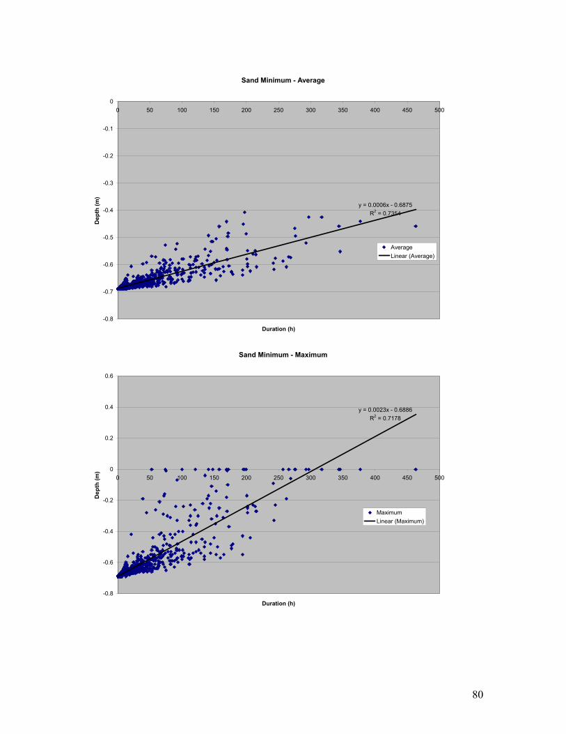
80
Sand Minimum - Average
y = 0.0006x - 0.6875R2 = 0.7354
-0.8
-0.7
-0.6
-0.5
-0.4
-0.3
-0.2
-0.1
00 50 100 150 200 250 300 350 400 450 500
Duration (h)
Dep
th (m
)
AverageLinear (Average)
Sand Minimum - Maximum
y = 0.0023x - 0.6886R2 = 0.7178
-0.8
-0.6
-0.4
-0.2
0
0.2
0.4
0.6
0 50 100 150 200 250 300 350 400 450 500
Duration (h)
Dep
th (m
)
MaximumLinear (Maximum)

81
Peat Maximum - Average
y = 0.001x - 0.6761R2 = 0.7477
-0.8
-0.7
-0.6
-0.5
-0.4
-0.3
-0.2
-0.1
00 50 100 150 200 250 300 350
Duration (h)
Dep
th (m
)
AverageLinear (Average)
Peat Maximum - Maximum
y = 0.0042x - 0.6568R2 = 0.6922
-0.8
-0.6
-0.4
-0.2
0
0.2
0.4
0.6
0.8
0 50 100 150 200 250 300 350
Duration (h)
Dep
th (m
)
MaximumLinear (Maximum)

82
Peat Average - Average
y = 0.0017x - 0.6614R2 = 0.623
-0.8
-0.7
-0.6
-0.5
-0.4
-0.3
-0.2
-0.1
00 50 100 150 200 250 300 350
Duration (h)
Dep
th (m
)
AverageLinear (Average)
Peat Average - Maximum
y = 0.0051x - 0.612R2 = 0.5223
-0.8
-0.6
-0.4
-0.2
0
0.2
0.4
0.6
0.8
1
1.2
0 50 100 150 200 250 300 350
Duration (h)
Dep
th (m
) MaximumLinear (Maximum)

83
Peat Minimum - Average
y = 0.0012x - 0.6549R2 = 0.3586
-0.8
-0.7
-0.6
-0.5
-0.4
-0.3
-0.2
-0.1
00 50 100 150 200 250 300 350
Duration (h)
Dep
th (m
)
AverageLinear (Average)
Peat Minimum - Maximum
y = 0.0047x - 0.615R2 = 0.4254
-0.8
-0.6
-0.4
-0.2
0
0.2
0.4
0.6
0.8
1
0 50 100 150 200 250 300 350
Duration (h)
Dep
th (m
)
MaximumLinear (Maximum)

84
Clay Maximum - Average
y = 0.0018x - 0.6594R2 = 0.5713
-0.8
-0.7
-0.6
-0.5
-0.4
-0.3
-0.2
-0.1
0
0.1
0 50 100 150 200 250 300 350 400 450
Duration (h)
Dep
th (m
)
AverageLinear (Average)
Clay Maximum - Maximum
y = 0.0053x - 0.6125R2 = 0.4948
-1
-0.5
0
0.5
1
1.5
2
0 50 100 150 200 250 300 350 400 450
Duration (h)
Dep
th (m
)
MaximumLinear (Maximum)
g

85
Clay Average - Average
y = 0.0017x - 0.6551R2 = 0.4824
-0.8
-0.7
-0.6
-0.5
-0.4
-0.3
-0.2
-0.1
0
0.1
0 50 100 150 200 250 300 350 400 450
Duration (h)
Dep
th (m
)
AverageLinear (Average)
Clay Average - Maximum
y = 0.0054x - 0.5968R2 = 0.4414
-1
-0.5
0
0.5
1
1.5
2
0 50 100 150 200 250 300 350 400 450
Duration (h)
Dep
th (m
)
MaximumLinear (Maximum)
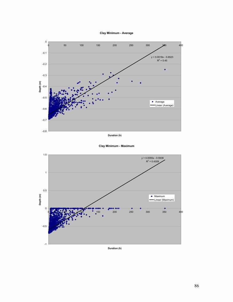
86
Clay Minimum - Average
y = 0.0018x - 0.6523R2 = 0.45
-0.8
-0.7
-0.6
-0.5
-0.4
-0.3
-0.2
-0.1
00 50 100 150 200 250 300 350 400
Duration (h)
Dep
th (m
)
AverageLinear (Average)
Clay Minimum - Maximum
y = 0.0055x - 0.5938R2 = 0.4309
-1
-0.5
0
0.5
1
1.5
0 50 100 150 200 250 300 350 400
Duration (h)
Dep
th (m
)
MaximumLinear (Maximum)
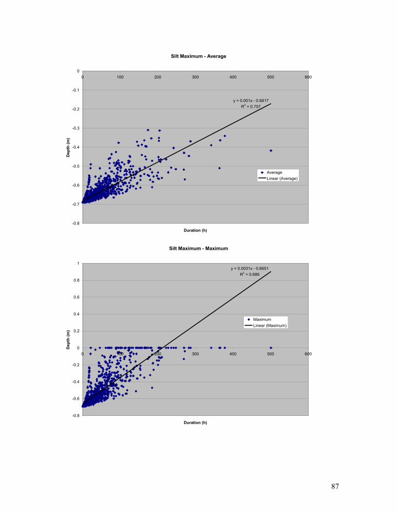
87
Silt Maximum - Average
y = 0.001x - 0.6817R2 = 0.707
-0.8
-0.7
-0.6
-0.5
-0.4
-0.3
-0.2
-0.1
00 100 200 300 400 500 600
Duration (h)
Dep
th (m
)
AverageLinear (Average)
Silt Maximum - Maximum
y = 0.0031x - 0.6651R2 = 0.686
-0.8
-0.6
-0.4
-0.2
0
0.2
0.4
0.6
0.8
1
0 100 200 300 400 500 600
Duration (h)
Dep
th (m
)
MaximumLinear (Maximum)
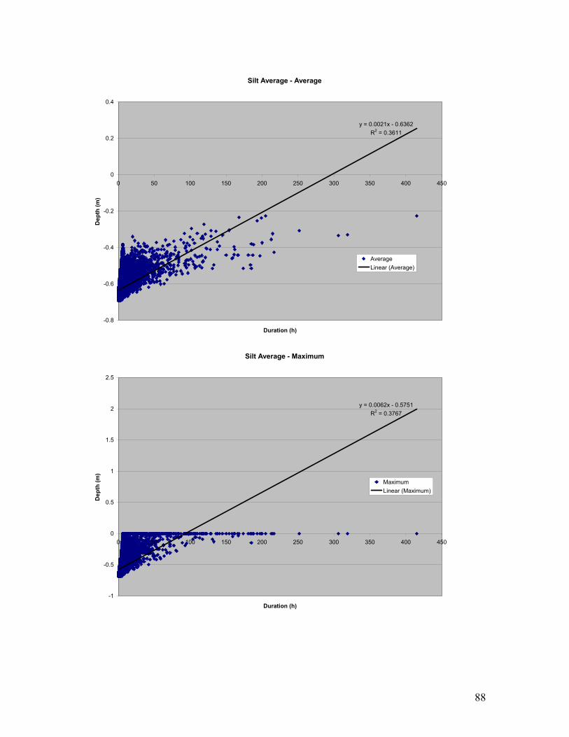
88
Silt Average - Average
y = 0.0021x - 0.6362R2 = 0.3611
-0.8
-0.6
-0.4
-0.2
0
0.2
0.4
0 50 100 150 200 250 300 350 400 450
Duration (h)
Dep
th (m
)
AverageLinear (Average)
Silt Average - Maximum
y = 0.0062x - 0.5751R2 = 0.3767
-1
-0.5
0
0.5
1
1.5
2
2.5
0 50 100 150 200 250 300 350 400 450
Duration (h)
Dep
th (m
)
MaximumLinear (Maximum)
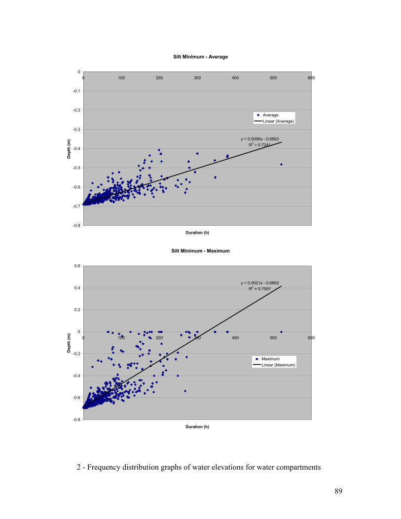
89
Silt Minimum - Average
y = 0.0006x - 0.6863R2 = 0.7241
-0.8
-0.7
-0.6
-0.5
-0.4
-0.3
-0.2
-0.1
00 100 200 300 400 500 600
Duration (h)
Dep
th (m
)
AverageLinear (Average)
Silt Minimum - Maximum
y = 0.0021x - 0.6862R2 = 0.7057
-0.8
-0.6
-0.4
-0.2
0
0.2
0.4
0.6
0 100 200 300 400 500 600
Duration (h)
Dep
th (m
)
MaximumLinear (Maximum)
2 - Frequency distribution graphs of water elevations for water compartments
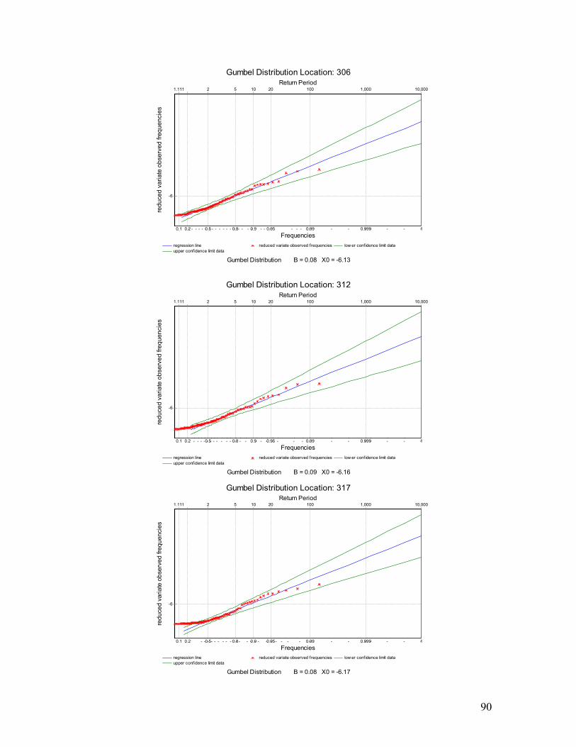
90
Gumbel Distribution Location: 312
Gumbel Distribution B = 0.09 X0 = -6.16
regression line reduced variate observed frequencies low er confidence limit dataupper confidence limit data
Frequencies0.1 0.2 0.5 0.8 0.9 0.95 0.99 0.999 1- - - - - - - - - - - - - - - - - - - - - - - - - - - - -
Return Period1.111 2 5 10 20 100 1,000 10,000
redu
ced
varia
te o
bser
ved
frequ
enci
es
-6
Gumbel Distribution Location: 317
Gumbel Distribution B = 0.08 X0 = -6.17
regression line reduced variate observed frequencies low er confidence limit dataupper confidence limit data
Frequencies0.1 0.2 0.5 0.8 0.9 0.95 0.99 0.999 1- - - - - - - - - - - - - - - - - - - - - - - - - - - - -
Return Period1.111 2 5 10 20 100 1,000 10,000
redu
ced
varia
te o
bser
ved
frequ
enci
es
-6
Gumbel Distribution Location: 306
Gumbel Distribution B = 0.08 X0 = -6.13
regression line reduced variate observed frequencies low er confidence limit dataupper confidence limit data
Frequencies0.1 0.2 0.5 0.8 0.9 0.95 0.99 0.999 1- - - - - - - - - - - - - - - - - - - - - - - - - - - - - - - -
Return Period1.111 2 5 10 20 100 1,000 10,000
redu
ced
varia
te o
bser
ved
frequ
enci
es
-6

91
Gumbel Distribution Location: 322
Gumbel Distribution B = 0.09 X0 = -6.07
regression line reduced variate observed frequencies low er confidence limit dataupper confidence limit data
Frequencies0.1 0.2 0.5 0.8 0.9 0.95 0.99 0.999 1- - - - - - - - - - - - - - - - - - - - - - - - - - - - - - - -
Return Period1.111 2 5 10 20 100 1,000 10,000
redu
ced
varia
te o
bser
ved
frequ
enci
es
-6
Gumbel Distribution Location: 325
Gumbel Distribution B = 0.07 X0 = -6.12
regression line reduced variate observed frequencies low er confidence limit dataupper confidence limit data
Frequencies0.1 0.2 0.5 0.8 0.9 0.95 0.99 0.999 1- - - - - - - - - - - - - - - - - - - - - - - - - - - - - -
Return Period1.111 2 5 10 20 100 1,000 10,000
redu
ced
varia
te o
bser
ved
frequ
enci
es
-5.3-5.35-5.4
-5.45-5.5
-5.55-5.6
-5.65-5.7
-5.75-5.8
-5.85-5.9
-5.95-6
-6.05-6.1
-6.15-6.2
Gumbel Distribution Location: 330
Gumbel Distribution B = 0.05 X0 = -5.94
regression line reduced variate observed frequencies low er confidence limit dataupper confidence limit data
Frequencies0.1 0.2 0.5 0.8 0.9 0.95 0.99 0.999 1- - - - - - - - - - - - - - - - - - - - - - - - - - - - - - -
Return Period1.111 2 5 10 20 100 1,000 10,000
redu
ced
varia
te o
bser
ved
frequ
enci
es
-5.4
-5.45
-5.5
-5.55
-5.6
-5.65
-5.7
-5.75
-5.8
-5.85
-5.9
-5.95
-6

92
Gumbel Distribution Location: 336
Gumbel Distribution B = 0.04 X0 = -5.94
regression line reduced variate observed frequencies low er confidence limit dataupper confidence limit data
Frequencies0.1 0.2 0.5 0.8 0.9 0.95 0.99 0.999 1- - - - - - - - - - - - - - - - - - - - - - - - - - - - - - - -
Return Period1.111 2 5 10 20 100 1,000 10,000
redu
ced
varia
te o
bser
ved
frequ
enci
es
-5.5
-5.55
-5.6
-5.65
-5.7
-5.75
-5.8
-5.85
-5.9
-5.95
-6
Gumbel Distribution Location: 337
Gumbel Distribution B = 0.10 X0 = -6.01
regression line reduced variate observed frequencies low er confidence limit dataupper confidence limit data
Frequencies0.1 0.2 0.5 0.8 0.9 0.95 0.99 0.999 1- - - - - - - - - - - - - - - - - - -
Return Period1.111 2 5 10 20 100 1,000 10,000
redu
ced
varia
te o
bser
ved
frequ
enci
es
-5
-6
Gumbel Distribution Location: 344
Gumbel Distribution B = 0.10 X0 = -6.00
regression line reduced variate observed frequencies low er confidence limit dataupper confidence limit data
Frequencies0.1 0.2 0.5 0.8 0.9 0.95 0.99 0.999 1- - - - - - - - - - - - - - - - - -
Return Period1.111 2 5 10 20 100 1,000 10,000
redu
ced
varia
te o
bser
ved
frequ
enci
es
-5
-6

93
Gumbel Distribution Location: 346
Gumbel Distribution B = 0.03 X0 = -5.92
regression line reduced variate observed frequencies low er confidence limit dataupper confidence limit data
Frequencies0.1 0.2 0.5 0.8 0.9 0.95 0.99 0.999 1- - - - - - - - - - - - - - - - - - - - - - - - - - - -
Return Period1.111 2 5 10 20 100 1,000 10,000
redu
ced
varia
te o
bser
ved
frequ
enci
es
-5.58-5.6
-5.62-5.64-5.66-5.68-5.7
-5.72-5.74-5.76-5.78-5.8
-5.82-5.84-5.86-5.88-5.9
-5.92-5.94-5.96-5.98
-6
Gumbel Distribution Location: 352
Gumbel Distribution B = 0.03 X0 = -3.14
regression line reduced variate observed frequencies low er confidence limit dataupper confidence limit data
Frequencies0.1 0.2 0.5 0.8 0.9 0.95 0.99 0.999 1- - - - - - - - - - - - - - - - - - - - - - - - - - - - -
Return Period1.111 2 5 10 20 100 1,000 10,000
redu
ced
varia
te o
bser
ved
frequ
enci
es
-2.84-2.86-2.88-2.9
-2.92-2.94-2.96-2.98
-3-3.02-3.04-3.06-3.08-3.1
-3.12-3.14-3.16-3.18-3.2
-3.22
Gumbel Distribution Location: 359
Gumbel Distribution B = 0.02 X0 = -3.20
regression line reduced variate observed frequencies low er confidence limit dataupper confidence limit data
Frequencies0.1 0.2 0.5 0.8 0.9 0.95 0.99 0.999 1- - - - - - - - - - - - - - - - - - - - - - - - - - - - - - -
Return Period1.111 2 5 10 20 100 1,000 10,000
redu
ced
varia
te o
bser
ved
frequ
enci
es
-2.94
-2.96
-2.98
-3
-3.02
-3.04
-3.06
-3.08
-3.1
-3.12
-3.14
-3.16
-3.18
-3.2
-3.22
-3.24
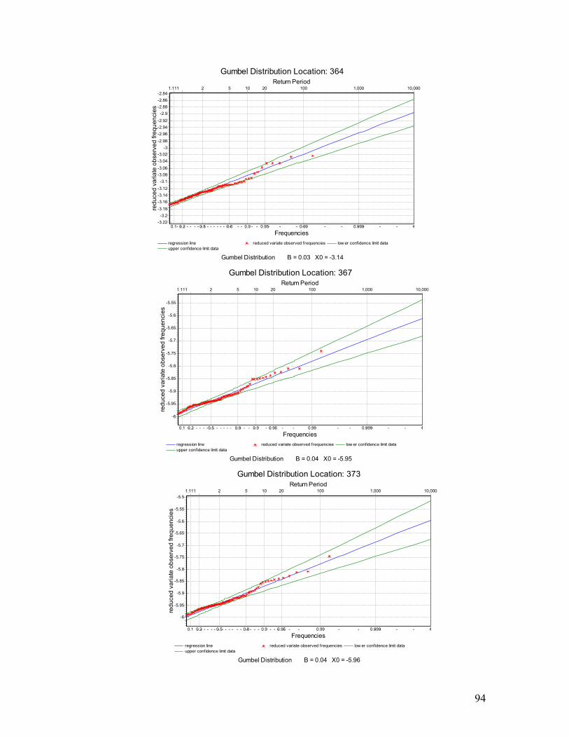
94
Gumbel Distribution Location: 364
Gumbel Distribution B = 0.03 X0 = -3.14
regression line reduced variate observed frequencies low er confidence limit dataupper confidence limit data
Frequencies0.1 0.2 0.5 0.8 0.9 0.95 0.99 0.999 1- - - - - - - - - - - - - - - - - - - - - - - - - - - - - - - -
Return Period1.111 2 5 10 20 100 1,000 10,000
redu
ced
varia
te o
bser
ved
frequ
enci
es
-2.84-2.86-2.88-2.9
-2.92-2.94-2.96-2.98
-3-3.02-3.04-3.06-3.08-3.1
-3.12-3.14-3.16-3.18-3.2
-3.22
Gumbel Distribution Location: 367
Gumbel Distribution B = 0.04 X0 = -5.95
regression line reduced variate observed frequencies low er confidence limit dataupper confidence limit data
Frequencies0.1 0.2 0.5 0.8 0.9 0.95 0.99 0.999 1- - - - - - - - - - - - - - - - - - - - - - - - - - - - - -
Return Period1.111 2 5 10 20 100 1,000 10,000
redu
ced
varia
te o
bser
ved
frequ
enci
es
-5.55
-5.6
-5.65
-5.7
-5.75
-5.8
-5.85
-5.9
-5.95
-6
Gumbel Distribution Location: 373
Gumbel Distribution B = 0.04 X0 = -5.96
regression line reduced variate observed frequencies low er confidence limit dataupper confidence limit data
Frequencies0.1 0.2 0.5 0.8 0.9 0.95 0.99 0.999 1- - - - - - - - - - - - - - - - - - - - - - - - - - - - - -
Return Period1.111 2 5 10 20 100 1,000 10,000
redu
ced
varia
te o
bser
ved
frequ
enci
es
-5.5
-5.55
-5.6
-5.65
-5.7
-5.75
-5.8
-5.85
-5.9
-5.95
-6

95
Gumbel Distribution Location: 377
Gumbel Distribution B = 0.05 X0 = -5.99
regression line reduced variate observed frequencies low er confidence limit dataupper confidence limit data
Frequencies0.1 0.2 0.5 0.8 0.9 0.95 0.99 0.999 1- - - - - - - - - - - - - - - - - - - - - - - - - - - -
Return Period1.111 2 5 10 20 100 1,000 10,000
redu
ced
varia
te o
bser
ved
frequ
enci
es
-5.45
-5.5
-5.55
-5.6
-5.65
-5.7
-5.75
-5.8
-5.85
-5.9
-5.95
-6
-6.05
Gumbel Distribution Location: 383
Gumbel Distribution B = 0.04 X0 = -5.28
regression line reduced variate observed frequencies low er confidence limit dataupper confidence limit data
Frequencies0.1 0.2 0.5 0.8 0.9 0.95 0.99 0.999 1- - - - - - - - - - - - - - - - - - - - - - - - - - - - - -
Return Period1.111 2 5 10 20 100 1,000 10,000
redu
ced
varia
te o
bser
ved
frequ
enci
es
-4.85
-4.9
-4.95
-5
-5.05
-5.1
-5.15
-5.2
-5.25
-5.3
-5.35
Gumbel Distribution Location: 385
Gumbel Distribution B = 0.04 X0 = -5.28
regression line reduced variate observed frequencies low er confidence limit dataupper confidence limit data
Frequencies0.1 0.2 0.5 0.8 0.9 0.95 0.99 0.999 1- - - - - - - - - - - - - - - - - - - - - - - - - - - - -
Return Period1.111 2 5 10 20 100 1,000 10,000
redu
ced
varia
te o
bser
ved
frequ
enci
es
-4.85
-4.9
-4.95
-5
-5.05
-5.1
-5.15
-5.2
-5.25
-5.3
-5.35

96
Gumbel Distribution Location: 395
Gumbel Distribution B = 0.04 X0 = -5.28
regression line reduced variate observed frequencies low er confidence limit dataupper confidence limit data
Frequencies0.1 0.2 0.5 0.8 0.9 0.95 0.99 0.999 1- - - - - - - - - - - - - - - - - - - - - - - - - - - - - -
Return Period1.111 2 5 10 20 100 1,000 10,000
redu
ced
varia
te o
bser
ved
frequ
enci
es
-4.85
-4.9
-4.95
-5
-5.05
-5.1
-5.15
-5.2
-5.25
-5.3
-5.35
Gumbel Distribution Location: 399
Gumbel Distribution B = 0.04 X0 = -5.36
regression line reduced variate observed frequencies low er confidence limit dataupper confidence limit data
Frequencies0.1 0.2 0.5 0.8 0.9 0.95 0.99 0.999 1- - - - - - - - - - - - - - - - - - - - - - - - - - - - - - - -
Return Period1.111 2 5 10 20 100 1,000 10,000
redu
ced
varia
te o
bser
ved
frequ
enci
es
-5
-5.05
-5.1
-5.15
-5.2
-5.25
-5.3
-5.35
-5.4
-5.45
Gumbel Distribution Location: 389
Gumbel Distribution B = 0.04 X0 = -5.28
regression line reduced variate observed frequencies low er confidence limit dataupper confidence limit data
Frequencies0.1 0.2 0.5 0.8 0.9 0.95 0.99 0.999 1- - - - - - - - - - - - - - - - - - - - - - - - - - - - -
Return Period1.111 2 5 10 20 100 1,000 10,000
redu
ced
varia
te o
bser
ved
frequ
enci
es
-4.85
-4.9
-4.95
-5
-5.05
-5.1
-5.15
-5.2
-5.25
-5.3
-5.35

97
Gumbel Distribution Location: 402
Gumbel Distribution B = 0.04 X0 = -5.35
regression line reduced variate observed frequencies low er confidence limit dataupper confidence limit data
Frequencies0.1 0.2 0.5 0.8 0.9 0.95 0.99 0.999 1- - - - - - - - - - - - - - - - - - - - - - - - - - - - - - - -
Return Period1.111 2 5 10 20 100 1,000 10,000
redu
ced
varia
te o
bser
ved
frequ
enci
es
-5
-5.05
-5.1
-5.15
-5.2
-5.25
-5.3
-5.35
-5.4
-5.45
Gumbel Distribution Location: 411
Gumbel Distribution B = 0.04 X0 = -2.83
regression line reduced variate observed frequencies low er confidence limit dataupper confidence limit data
Frequencies0.1 0.2 0.5 0.8 0.9 0.95 0.99 0.999 1- - - - - - - - - - - - - - - - - - - - - - - - - - - - - - - -
Return Period1.111 2 5 10 20 100 1,000 10,000
redu
ced
varia
te o
bser
ved
frequ
enci
es
-2.4
-2.45
-2.5
-2.55
-2.6
-2.65
-2.7
-2.75
-2.8
-2.85
-2.9
-2.95
Gumbel Distribution Location: 407
Gumbel Distribution B = 0.05 X0 = -3.04
regression line reduced variate observed frequencies low er conf idence limit dataupper confidence limit data
Frequencies0.1 0.2 0.5 0.8 0.9 0.95 0.99 0.999 1- - - - - - - - - - - - - - - - - - - - - - - - - - - - - - - - - -
Return Period1.111 2 5 10 20 100 1,000 10,000
redu
ced
varia
te o
bser
ved
frequ
enci
es
-2.55
-2.6
-2.65
-2.7
-2.75
-2.8
-2.85
-2.9
-2.95
-3
-3.05
-3.1
-3.15

98
Gumbel Distribution Location: 419
Gumbel Distribution B = 0.01 X0 = -3.17
regression line reduced variate observed frequencies low er confidence limit dataupper confidence limit data
Frequencies0.1 0.2 0.5 0.8 0.9 0.95 0.99 0.999 1- - - - - - - - - - - - - - - - - - - - - - - - - - - - - - - - -
Return Period1.111 2 5 10 20 100 1,000 10,000
redu
ced
varia
te o
bser
ved
frequ
enci
es
-3.09
-3.1
-3.11
-3.12
-3.13
-3.14
-3.15
-3.16
-3.17
-3.18
-3.19
Gumbel Distribution Location: 414
Gumbel Distribution B = 0.04 X0 = -5.27
regression line reduced variate observed frequencies low er confidence limit dataupper confidence limit data
Frequencies0.1 0.2 0.5 0.8 0.9 0.95 0.99 0.999 1- - - - - - - - - - - - - - - - - - - - - - - - - - - - - - -
Return Period1.111 2 5 10 20 100 1,000 10,000
redu
ced
varia
te o
bser
ved
frequ
enci
es
-4.8
-4.85
-4.9
-4.95
-5
-5.05
-5.1
-5.15
-5.2
-5.25
-5.3
-5.35
Gumbel Distribution Location: 423
Gumbel Distribution B = 0.11 X0 = -5.95
regression line reduced variate observed frequencies low er confidence limit dataupper confidence limit data
Frequencies0.1 0.2 0.5 0.8 0.9 0.95 0.99 0.999 1- - - - - - - - - - - - - - - - - - - - -
Return Period1.111 2 5 10 20 100 1,000 10,000
redu
ced
varia
te o
bser
ved
frequ
enci
es
-5
-6
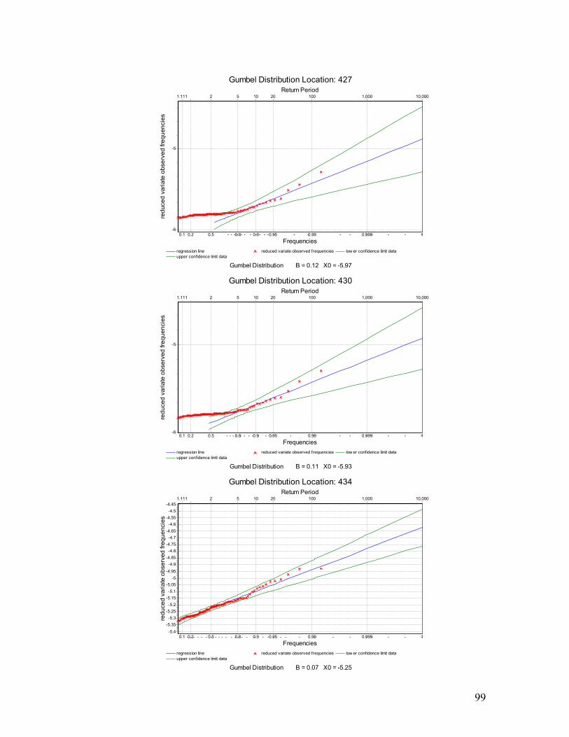
99
Gumbel Distribution Location: 427
Gumbel Distribution B = 0.12 X0 = -5.97
regression line reduced variate observed frequencies low er confidence limit dataupper confidence limit data
Frequencies0.1 0.2 0.5 0.8 0.9 0.95 0.99 0.999 1- - - - - - - - - - - - - - - - - - - - -
Return Period1.111 2 5 10 20 100 1,000 10,000
redu
ced
varia
te o
bser
ved
frequ
enci
es
-5
-6
Gumbel Distribution Location: 430
Gumbel Distribution B = 0.11 X0 = -5.93
regression line reduced variate observed frequencies low er confidence limit dataupper confidence limit data
Frequencies0.1 0.2 0.5 0.8 0.9 0.95 0.99 0.999 1- - - - - - - - - - - - - - - - - - - -
Return Period1.111 2 5 10 20 100 1,000 10,000
redu
ced
varia
te o
bser
ved
frequ
enci
es
-5
-6
Gumbel Distribution Location: 434
Gumbel Distribution B = 0.07 X0 = -5.25
regression line reduced variate observed frequencies low er confidence limit dataupper confidence limit data
Frequencies0.1 0.2 0.5 0.8 0.9 0.95 0.99 0.999 1- - - - - - - - - - - - - - - - - - - - - - - - - - - - - - -
Return Period1.111 2 5 10 20 100 1,000 10,000
redu
ced
varia
te o
bser
ved
frequ
enci
es
-4.45-4.5
-4.55-4.6
-4.65-4.7
-4.75-4.8
-4.85-4.9
-4.95-5
-5.05-5.1
-5.15-5.2
-5.25-5.3
-5.35-5.4

100
3 -Script designed for WB21 model Option Compare Database Option Base 1 Sub wb21() Dim time1 c1bouwspring = Array(8 * 10 ^ -5, 9 * 10 ^ -5, 8 * 10 ^ -5, 9 * 10 ^ -5, 10 * 10 ^ -5) c1bouwsummer = Array(14 * 10 ^ -5, 15 * 10 ^ -5, 14 * 10 ^ -5, 16 * 10 ^ -5, 16 * 10 ^ -5) c1bouwautumn = Array(7 * 10 ^ -5, 7 * 10 ^ -5, 7 * 10 ^ -5, 8 * 10 ^ -5, 8 * 10 ^ -5) c1bouwwinter = Array(0, 0, 0, 0, 0) c0spring = Array(20 * 10 ^ -5, 10 * 10 ^ -5, 5 * 10 ^ -5, 10 * 10 ^ -5, 0) c0summer = Array(26 * 10 ^ -5, 17 * 10 ^ -5, 17 * 10 ^ -5, 17 * 10 ^ -5, 0) c0autumn = Array(6 * 10 ^ -5, 6 * 10 ^ -5, 8 * 10 ^ -5, 6 * 10 ^ -5, 0) c0winter = Array(0, 0, 0, 0, 0) c1hoogspring = Array(14 * 10 ^ -5, 14 * 10 ^ -5, 14 * 10 ^ -5, 16 * 10 ^ -5, 16 * 10 ^ -5) c1hoogsummer = Array(24 * 10 ^ -5, 24 * 10 ^ -5, 23 * 10 ^ -5, 27 * 10 ^ -5, 27 * 10 ^ -5) c1hoogautumn = Array(11 * 10 ^ -5, 12 * 10 ^ -5, 11 * 10 ^ -5, 13 * 10 ^ -5, 13 * 10 ^ -5) c1hoogwinter = Array(0, 0, 0, 0, 0) c2rest = Array(21 * 10 ^ -5, 21 * 10 ^ -5, 21 * 10 ^ -5, 7 * 10 ^ -5, 5 * 10 ^ -5) c2winter = Array(0, 0, 0, 0, 0) Maximumdamage = Array(900, 3600, 18000) Dim wc(40) As Variant Dim compdamage(40) As Variant nodenumber2 = 0 time1 = 0 hmax = -100 level1 = -100 hsum = 0 dursum = 0 eventsum = 0 location = 0 duration = 0 eventsum = 0 eventspring = 0 eventsummer = 0 eventautumn = 0 eventwinter = 0 durspring = 0 dursummer = 0 durautumn = 0 durwinter = 0 skowcount = 0 sowcount = 0 durationexceedcount = 0 damagefuncskow = 0 damagefuncsow = 0 damagefuncduration = 0 yearlydamageagg = 0 yearlydamagegrass = 0 nodecount = 1 Open "d:\berkeldin.txt" For Binary As #1 Open "d:\berkeldout.txt" For Output As #2 Open "d:\berkeldstat.txt" For Output As #3 Do While location < LOF(1) Input #1, nodenumber1, month1, level location = Loc(1) time1 = time1 + 1 year1 = time1 / 365
101
If nodenumber1 <> nodenumber2 Then If nodenumber2 <> 0 Then Print #2, "-----------------------------------------------------------------" Print #2, Print #2, "*Location:"; nodenumber2 Print #2, "*Water compartment:"; watercomp Print #2, Print #2, "*Number of events:"; eventsum Print #2, Print #2, "*Number of events in spring:"; eventspring Print #2, "*Number of events in summer:"; eventsummer Print #2, "*Number of events in autumn:"; eventautumn Print #2, "*Number of events in winter:"; eventwinter Print #2, Print #2, "*Duration of events in spring:"; durspring Print #2, "*Duration of events in summer:"; dursummer Print #2, "*Duration of events in autumn:"; durautumn Print #2, "*Duration of events in winter:"; durwinter Print #2, Print #2, "*Number of events calculated by skow:"; skowcount Print #2, "*Number of events calculated by sow:"; sowcount Print #2, "*Number of events exceeding 3 days:"; durationexceedcount Print #2, Print #2, "*Damage function sum calculated by skow:"; damagefuncskow Print #2, "*Damage function sum calculated by sow:"; damagefuncsow Print #2, "*Damage function sum calculated due to duration exceeding 3 days:"; damagefuncduration Print #2, Print #2, "*Total duration above target level:"; dursum Print #2, "*Total simulation period in days:"; time1 Print #2, "*Total simulation period in years:"; year1 Print #2, Print #2, "*Total damage function for grass:"; damagefuncsumgrass Print #2, "*Total damage function for aggriculture:"; damagefuncsumagg Print #2, Print #2, "*Total damage for grass:"; totaldamagegrass Print #2, "*Total damage for aggriculture;"; totaldamageagg Print #2, "*Total damage:"; totaldamage Print #2, "*Anual avarage risk:"; anualaverage Print #2, Print #2, "-----------------------------------------------------------------" Print #3, "-----------------------------------------------------------------" Print #3, Print #3, "*Location:"; nodenumber2 Print #3, "*Water compartment:"; watercomp Print #3, Print #3, "*Number of events:"; eventsum Print #3, Print #3, "*Number of events in spring:"; eventspring Print #3, "*Number of events in summer:"; eventsummer Print #3, "*Number of events in autumn:"; eventautumn Print #3, "*Number of events in winter:"; eventwinter Print #3, Print #3, "*Duration of events in spring:"; durspring Print #3, "*Duration of events in summer:"; dursummer Print #3, "*Duration of events in autumn:"; durautumn Print #3, "*Duration of events in winter:"; durwinter Print #3, Print #3, "*Number of events calculated by skow:"; skowcount Print #3, "*Number of events calculated by sow:"; sowcount Print #3, "*Number of events exceeding 3 days:"; durationexceedcount Print #3, Print #3, "*Damage function sum calculated by skow:"; damagefuncskow Print #3, "*Damage function sum calculated by sow:"; damagefuncsow Print #3, "*Damage function sum calculated due to duration exceeding 3 days:"; damagefuncduration Print #3, Print #3, "*Total duration above target level:"; dursum Print #3, "*Total simulation period in days:"; time1

102
Print #3, "*Total simulation period in years:"; year1 Print #3, Print #3, "*Total damage function for grass:"; damagefuncsumgrass Print #3, "*Total damage function for aggriculture:"; damagefuncsumagg Print #3, Print #3, "*Total damage for grass:"; totaldamagegrass Print #3, "*Total damage for aggriculture;"; totaldamageagg Print #3, "*Total damage:"; totaldamage Print #3, "*Anual avarage risk:"; anualaverage Print #3, Print #3, "-----------------------------------------------------------------" wc(nodecount) = watercomp compdamage(nodecount) = anualaverage nodecount = nodecount + 1 End If Print #2, "*Duration", "Height", "Mode", "Damage Coefficient Aggriculture", "Damage Coefficient Grass" nodenumber2 = nodenumber1 eventsum = 0 eventspring = 0 eventsummer = 0 eventautumn = 0 eventwinter = 0 durspring = 0 dursummer = 0 durautumn = 0 durwinter = 0 skowcount = 0 sowcount = 0 durationexceedcount = 0 damagefuncskow = 0 damagefuncsow = 0 damagefuncduration = 0 dursum = 0 time1 = 1 damagefuncsumgrass = 0 damagefuncsumagg = 0 totaldamage = 0 'coef = Array(%grass, soiltype, targetlevel, area, %aggriculture, watercompartment) 'soil type 1=zand or leermarm 2=lichte zavel/lemig 3=zware zawel/moerige 4=lichte klei 5=zware klei If nodenumber1 = 288 Then coef = Array(0.289, 4, -5.3, 135.75, 0.248, 306) If nodenumber1 = 292 Then coef = Array(0.682, 4, -5.29, 78.56, 0.086, 344) If nodenumber1 = 309 Then coef = Array(0.275, 4, -5.32, 100.56, 0.144, 312) If nodenumber1 = 315 Then coef = Array(0.646, 4, -5.27, 82.63, 0.161, 317) If nodenumber1 = 321 Then coef = Array(0.558, 4, -5.48, 78.38, 0.436, 322) If nodenumber1 = 323 Then coef = Array(0.172, 4, -3.84, 95, 0, 325) If nodenumber1 = 328 Then coef = Array(0.263, 2, -5.19, 55.69, 0, 330) If nodenumber1 = 333 Then coef = Array(0.252, 4, -5.14, 30.75, 0, 336) If nodenumber1 = 338 Then coef = Array(0.575, 4, -4.88, 49.25, 0.056, 337) If nodenumber1 = 348 Then coef = Array(0.678, 4, -4.69, 120.25, 0.012, 346) If nodenumber1 = 354 Then coef = Array(0.513, 4, -2.68, 55.56, 0.141, 352) If nodenumber1 = 358 Then coef = Array(0.277, 4, -2.65, 27.56, 0, 359) If nodenumber1 = 362 Then coef = Array(0.474, 4, -2.93, 22.81, 0, 364) If nodenumber1 = 369 Then coef = Array(0.291, 4, -2.56, 24.5, 0, 367) If nodenumber1 = 370 Then coef = Array(0.459, 4, -5.3, 80.19, 0.084, 373) If nodenumber1 = 375 Then coef = Array(0.636, 4, -5.27, 66.75, 0.155, 377) If nodenumber1 = 381 Then coef = Array(0.495, 4, -4.84, 40.94, 0.011, 383) If nodenumber1 = 386 Then coef = Array(0.891, 4, -5.18, 50, 0, 385) If nodenumber1 = 392 Then coef = Array(0.565, 2, -5.01, 51.06, 0.174, 389) If nodenumber1 = 393 Then coef = Array(0.864, 4, -5.02, 33.06, 0, 395) If nodenumber1 = 397 Then coef = Array(0.609, 2, -4.97, 84.63, 0.077, 399) If nodenumber1 = 403 Then coef = Array(0.745, 4, -4.64, 67.69, 0.01, 402) If nodenumber1 = 406 Then coef = Array(0.555, 4, -2.87, 94.81, 0.042, 407) If nodenumber1 = 409 Then coef = Array(0.47, 4, -2.77, 116.56, 0.064, 411) If nodenumber1 = 415 Then coef = Array(0.902, 2, -5.03, 35.25, 0, 414)
103
If nodenumber1 = 418 Then coef = Array(0.701, 2, -2.98, 41.19, 0, 419) If nodenumber1 = 424 Then coef = Array(0.699, 2, -5.32, 57.5, 0.061, 423) If nodenumber1 = 425 Then coef = Array(0.783, 2, -5.22, 81.75, 0.038, 427) If nodenumber1 = 431 Then coef = Array(0.945, 2, -5.39, 94.38, 0.054, 430) If nodenumber1 = 432 Then coef = Array(0.873, 2, -5.12, 99.56, 0, 434) If nodenumber1 = 467 Then coef = Array(0, 2, -9, 0, 0, 470) watercomp = coef(6) End If If level > coef(3) Then height1 = level - coef(3) duration = duration + 1 hsum = hsum + height1 level1 = level If hmax < height1 Then hmax = height1 End If If level < coef(3) And level1 > coef(3) Then havgr = hsum / duration sow = hmax * duration * 100 skow = hmax * hmax * duration * 10000 If month1 > 2 And month1 < 6 Then durspring = durspring + duration eventspring = eventspring + 1 c0 = c0spring(coef(2)) c1b = c1bouwspring(coef(2)) c1h = c1hoogspring(coef(2)) c2 = c2rest(coef(2)) End If If month1 > 5 And month1 < 9 Then dursummer = dursummer + duration eventsummer = eventsummer + 1 c0 = c0summer(coef(2)) c1b = c1bouwsummer(coef(2)) c1h = c1hoogsummer(coef(2)) c2 = c2rest(coef(2)) End If If month1 > 8 And month1 < 11 Then durautumn = durautumn + duration eventautumn = eventautumn + 1 c0 = c0autumn(coef(2)) c1b = c1bouwautumn(coef(2)) c1h = c1hoogautumn(coef(2)) c2 = c2rest(coef(2)) End If If month1 > 10 Or month1 < 3 Then durwinter = durwinter + duration eventwinter = eventwinter + 1 c0 = c0winter(coef(2)) c1b = c1bouwwinter(coef(2)) c1h = c1hoogwinter(coef(2)) c2 = c2winter(coef(2)) End If 'grass damage damagefuncgrass = c0 * sow yearlydamagegrass = yearlydamagegrass + damagefuncgrass If yearlydamagegrass > 1 Then yearlydamagegrass = 1 'aggricultural damage

104
d1 = c1b * sow d2 = c2 * skow If d1 > d2 Then damagefuncagg = d1 Else damagefuncagg = d2 If damagefuncagg = c2 * skow Then skowcount = skowcount + 1 If damagefuncagg > 1 Then damagefuncagg = 1 damagefuncskow = damagefuncskow + damagefuncagg Mode = "skow" End If If duration >= 4 Then durationexceedcount = durationexceedcount + 1 End If If damagefuncagg <> c2 * skow And damagefuncagg <> 1 Then sowcount = sowcount + 1 If damagefuncagg > 1 Then damagefuncagg = 1 damagefuncsow = damagefuncsow + damagefuncagg Mode = "sow" End If yearlydamageagg = yearlydamageagg + damagefuncagg If yearlydamageagg > 1 Then yearlydamageagg = 1 Print #2, duration; Tab; hmax; Tab; Mode; Tab; damagefuncagg; Tab; damagefuncgrass eventsum = eventsum + 1 dursum = dursum + duration duration = 0 hsum = 0 hmax = -100 level1 = -100 damagefuncgrass = 0 damagefuncagg = 0 End If If month1 = 1 Then damagefuncsumgrass = damagefuncsumgrass + yearlydamagegrass yearlydamagegrass = 0 damagefuncsumagg = damagefuncsumagg + yearlydamageagg yearlydamageagg = 0 End If totaldamagegrass = damagefuncsumgrass * coef(1) * coef(4) * 900 totaldamageagg = damagefuncsumagg * coef(5) * coef(4) * 3600 totaldamage = (damagefuncsumgrass * coef(1) * coef(4) * 900) + (damagefuncsumagg * coef(5) * coef(4) * 3600) anualaverage = totaldamage / year1 Loop 'final summary print Print #3, Print #3, "Water Compartment"; Tab; "Anual Damage" i = 1 Do While i <= 38 Print #3, wc(i); Tab; compdamage(i) i = i + 1 Loop Close #1 Close #2 Close #3

105
----------------------------------------------------------------- *Location: 288 *Water compartment: 306 *Number of events: 7 *Number of events in spring: 1 *Number of events in summer: 1 *Number of events in autumn: 2 *Number of events in winter: 3 *Duration of events in spring: 1 *Duration of events in summer: 1 *Duration of events in autumn: 3 *Duration of events in winter: 5 *Number of events calculated by skow: 7 *Number of events calculated by sow: 0 *Number of events exceeding 3 days: 0 *Damage function sum calculated by skow: 0.1666 *Damage function sum calculated by sow: 0 *Damage function sum calculated due to duration exceeding 3 days: 0 *Total duration above target level: 10 *Total simulation period in days: 36527 *Total simulation period in years: 100.07397260274 *Total damage function for grass: 0.0092 *Total damage function for aggriculture: 0.1666 *Total damage for grass: 324.83889 *Total damage for aggriculture; 20191.52016 *Total damage: 20516.35905 *Anual avarage risk: 205.017550600942 ----------------------------------------------------------------- ----------------------------------------------------------------- *Location: 292 *Water compartment: 344 *Number of events: 592 *Number of events in spring: 58 *Number of events in summer: 68 *Number of events in autumn: 114 *Number of events in winter: 352 *Duration of events in spring: 109 *Duration of events in summer: 128 *Duration of events in autumn: 280 *Duration of events in winter: 895 *Number of events calculated by skow: 577 *Number of events calculated by sow: 15 *Number of events exceeding 3 days: 113 *Damage function sum calculated by skow: 23.2173 *Damage function sum calculated by sow: 0.00164 *Damage function sum calculated due to duration exceeding 3 days: 0 *Total duration above target level: 1412 *Total simulation period in days: 36527 *Total simulation period in years: 100.07397260274 *Total damage function for grass: 1.1537 *Total damage function for aggriculture: 23.1328 *Total damage for grass: 55631.5616736 *Total damage for aggriculture; 562640.0329728 *Total damage: 618271.5946464 *Anual avarage risk: 6178.31495498921 -----------------------------------------------------------------
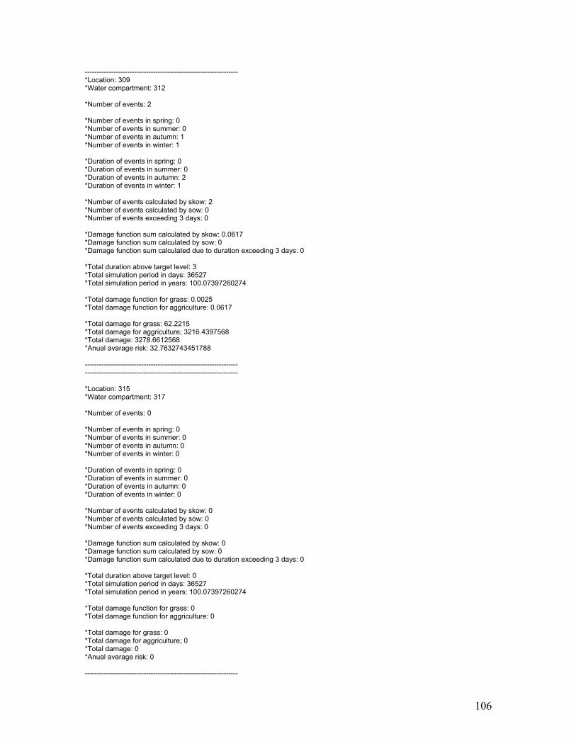
106
----------------------------------------------------------------- *Location: 309 *Water compartment: 312 *Number of events: 2 *Number of events in spring: 0 *Number of events in summer: 0 *Number of events in autumn: 1 *Number of events in winter: 1 *Duration of events in spring: 0 *Duration of events in summer: 0 *Duration of events in autumn: 2 *Duration of events in winter: 1 *Number of events calculated by skow: 2 *Number of events calculated by sow: 0 *Number of events exceeding 3 days: 0 *Damage function sum calculated by skow: 0.0617 *Damage function sum calculated by sow: 0 *Damage function sum calculated due to duration exceeding 3 days: 0 *Total duration above target level: 3 *Total simulation period in days: 36527 *Total simulation period in years: 100.07397260274 *Total damage function for grass: 0.0025 *Total damage function for aggriculture: 0.0617 *Total damage for grass: 62.2215 *Total damage for aggriculture; 3216.4397568 *Total damage: 3278.6612568 *Anual avarage risk: 32.7632743451788 ----------------------------------------------------------------- ----------------------------------------------------------------- *Location: 315 *Water compartment: 317 *Number of events: 0 *Number of events in spring: 0 *Number of events in summer: 0 *Number of events in autumn: 0 *Number of events in winter: 0 *Duration of events in spring: 0 *Duration of events in summer: 0 *Duration of events in autumn: 0 *Duration of events in winter: 0 *Number of events calculated by skow: 0 *Number of events calculated by sow: 0 *Number of events exceeding 3 days: 0 *Damage function sum calculated by skow: 0 *Damage function sum calculated by sow: 0 *Damage function sum calculated due to duration exceeding 3 days: 0 *Total duration above target level: 0 *Total simulation period in days: 36527 *Total simulation period in years: 100.07397260274 *Total damage function for grass: 0 *Total damage function for aggriculture: 0 *Total damage for grass: 0 *Total damage for aggriculture; 0 *Total damage: 0 *Anual avarage risk: 0 -----------------------------------------------------------------

107
----------------------------------------------------------------- *Location: 321 *Water compartment: 322 *Number of events: 1 *Number of events in spring: 0 *Number of events in summer: 0 *Number of events in autumn: 1 *Number of events in winter: 0 *Duration of events in spring: 0 *Duration of events in summer: 0 *Duration of events in autumn: 1 *Duration of events in winter: 0 *Number of events calculated by skow: 1 *Number of events calculated by sow: 0 *Number of events exceeding 3 days: 0 *Damage function sum calculated by skow: 0.00567 *Damage function sum calculated by sow: 0 *Damage function sum calculated due to duration exceeding 3 days: 0 *Total duration above target level: 1 *Total simulation period in days: 36527 *Total simulation period in years: 100.07397260274 *Total damage function for grass: 0.00054 *Total damage function for aggriculture: 0.00567 *Total damage for grass: 21.25571544 *Total damage for aggriculture; 697.55315616 *Total damage: 718.8088716 *Anual avarage risk: 7.18297207835515 ----------------------------------------------------------------- ----------------------------------------------------------------- *Location: 323 *Water compartment: 325 *Number of events: 0 *Number of events in spring: 0 *Number of events in summer: 0 *Number of events in autumn: 0 *Number of events in winter: 0 *Duration of events in spring: 0 *Duration of events in summer: 0 *Duration of events in autumn: 0 *Duration of events in winter: 0 *Number of events calculated by skow: 0 *Number of events calculated by sow: 0 *Number of events exceeding 3 days: 0 *Damage function sum calculated by skow: 0 *Damage function sum calculated by sow: 0 *Damage function sum calculated due to duration exceeding 3 days: 0 *Total duration above target level: 0 *Total simulation period in days: 36527 *Total simulation period in years: 100.07397260274 *Total damage function for grass: 0 *Total damage function for aggriculture: 0 *Total damage for grass: 0 *Total damage for aggriculture; 0 *Total damage: 0 *Anual avarage risk: 0 -----------------------------------------------------------------
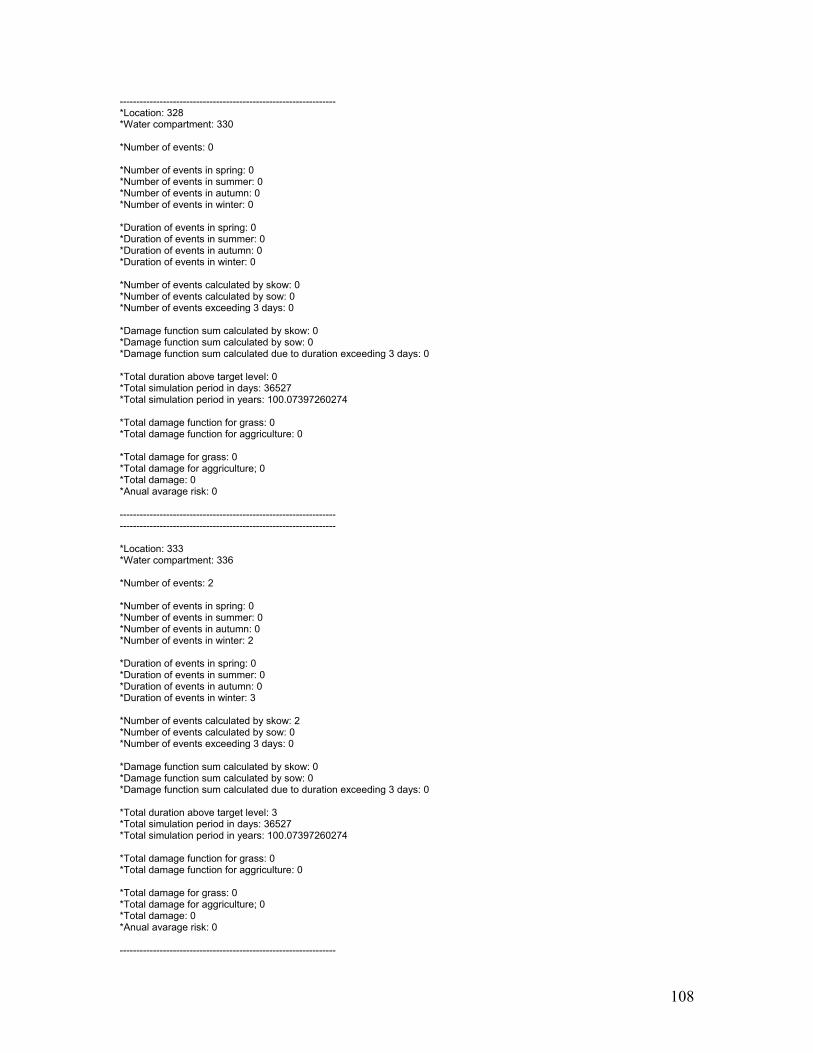
108
----------------------------------------------------------------- *Location: 328 *Water compartment: 330 *Number of events: 0 *Number of events in spring: 0 *Number of events in summer: 0 *Number of events in autumn: 0 *Number of events in winter: 0 *Duration of events in spring: 0 *Duration of events in summer: 0 *Duration of events in autumn: 0 *Duration of events in winter: 0 *Number of events calculated by skow: 0 *Number of events calculated by sow: 0 *Number of events exceeding 3 days: 0 *Damage function sum calculated by skow: 0 *Damage function sum calculated by sow: 0 *Damage function sum calculated due to duration exceeding 3 days: 0 *Total duration above target level: 0 *Total simulation period in days: 36527 *Total simulation period in years: 100.07397260274 *Total damage function for grass: 0 *Total damage function for aggriculture: 0 *Total damage for grass: 0 *Total damage for aggriculture; 0 *Total damage: 0 *Anual avarage risk: 0 ----------------------------------------------------------------- ----------------------------------------------------------------- *Location: 333 *Water compartment: 336 *Number of events: 2 *Number of events in spring: 0 *Number of events in summer: 0 *Number of events in autumn: 0 *Number of events in winter: 2 *Duration of events in spring: 0 *Duration of events in summer: 0 *Duration of events in autumn: 0 *Duration of events in winter: 3 *Number of events calculated by skow: 2 *Number of events calculated by sow: 0 *Number of events exceeding 3 days: 0 *Damage function sum calculated by skow: 0 *Damage function sum calculated by sow: 0 *Damage function sum calculated due to duration exceeding 3 days: 0 *Total duration above target level: 3 *Total simulation period in days: 36527 *Total simulation period in years: 100.07397260274 *Total damage function for grass: 0 *Total damage function for aggriculture: 0 *Total damage for grass: 0 *Total damage for aggriculture; 0 *Total damage: 0 *Anual avarage risk: 0 -----------------------------------------------------------------

109
----------------------------------------------------------------- *Location: 338 *Water compartment: 337 *Number of events: 0 *Number of events in spring: 0 *Number of events in summer: 0 *Number of events in autumn: 0 *Number of events in winter: 0 *Duration of events in spring: 0 *Duration of events in summer: 0 *Duration of events in autumn: 0 *Duration of events in winter: 0 *Number of events calculated by skow: 0 *Number of events calculated by sow: 0 *Number of events exceeding 3 days: 0 *Damage function sum calculated by skow: 0 *Damage function sum calculated by sow: 0 *Damage function sum calculated due to duration exceeding 3 days: 0 *Total duration above target level: 0 *Total simulation period in days: 36527 *Total simulation period in years: 100.07397260274 *Total damage function for grass: 0 *Total damage function for aggriculture: 0 *Total damage for grass: 0 *Total damage for aggriculture; 0 *Total damage: 0 *Anual avarage risk: 0 ----------------------------------------------------------------- ----------------------------------------------------------------- *Location: 348 *Water compartment: 346 *Number of events: 0 *Number of events in spring: 0 *Number of events in summer: 0 *Number of events in autumn: 0 *Number of events in winter: 0 *Duration of events in spring: 0 *Duration of events in summer: 0 *Duration of events in autumn: 0 *Duration of events in winter: 0 *Number of events calculated by skow: 0 *Number of events calculated by sow: 0 *Number of events exceeding 3 days: 0 *Damage function sum calculated by skow: 0 *Damage function sum calculated by sow: 0 *Damage function sum calculated due to duration exceeding 3 days: 0 *Total duration above target level: 0 *Total simulation period in days: 36527 *Total simulation period in years: 100.07397260274 *Total damage function for grass: 0 *Total damage function for aggriculture: 0 *Total damage for grass: 0 *Total damage for aggriculture; 0 *Total damage: 0 *Anual avarage risk: 0 -----------------------------------------------------------------
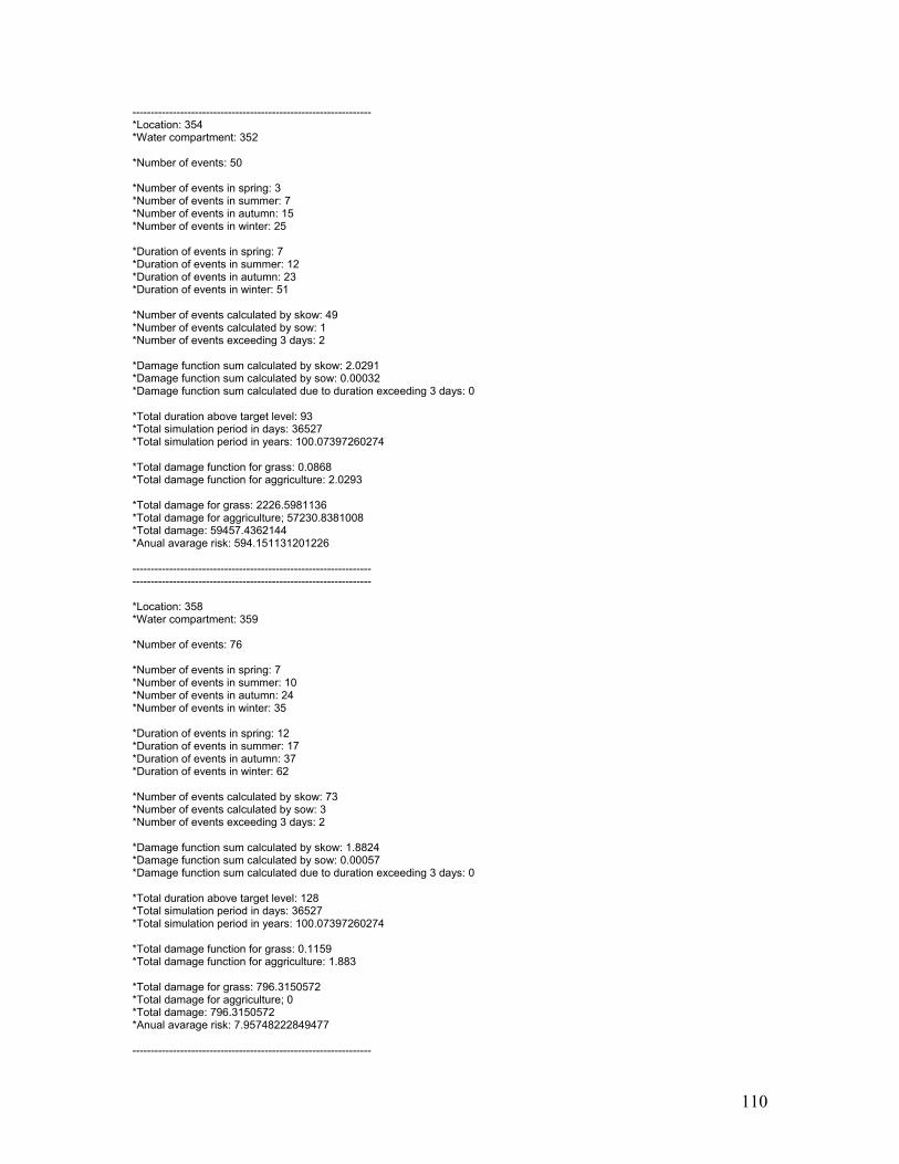
110
----------------------------------------------------------------- *Location: 354 *Water compartment: 352 *Number of events: 50 *Number of events in spring: 3 *Number of events in summer: 7 *Number of events in autumn: 15 *Number of events in winter: 25 *Duration of events in spring: 7 *Duration of events in summer: 12 *Duration of events in autumn: 23 *Duration of events in winter: 51 *Number of events calculated by skow: 49 *Number of events calculated by sow: 1 *Number of events exceeding 3 days: 2 *Damage function sum calculated by skow: 2.0291 *Damage function sum calculated by sow: 0.00032 *Damage function sum calculated due to duration exceeding 3 days: 0 *Total duration above target level: 93 *Total simulation period in days: 36527 *Total simulation period in years: 100.07397260274 *Total damage function for grass: 0.0868 *Total damage function for aggriculture: 2.0293 *Total damage for grass: 2226.5981136 *Total damage for aggriculture; 57230.8381008 *Total damage: 59457.4362144 *Anual avarage risk: 594.151131201226 ----------------------------------------------------------------- ----------------------------------------------------------------- *Location: 358 *Water compartment: 359 *Number of events: 76 *Number of events in spring: 7 *Number of events in summer: 10 *Number of events in autumn: 24 *Number of events in winter: 35 *Duration of events in spring: 12 *Duration of events in summer: 17 *Duration of events in autumn: 37 *Duration of events in winter: 62 *Number of events calculated by skow: 73 *Number of events calculated by sow: 3 *Number of events exceeding 3 days: 2 *Damage function sum calculated by skow: 1.8824 *Damage function sum calculated by sow: 0.00057 *Damage function sum calculated due to duration exceeding 3 days: 0 *Total duration above target level: 128 *Total simulation period in days: 36527 *Total simulation period in years: 100.07397260274 *Total damage function for grass: 0.1159 *Total damage function for aggriculture: 1.883 *Total damage for grass: 796.3150572 *Total damage for aggriculture; 0 *Total damage: 796.3150572 *Anual avarage risk: 7.95748222849477 -----------------------------------------------------------------
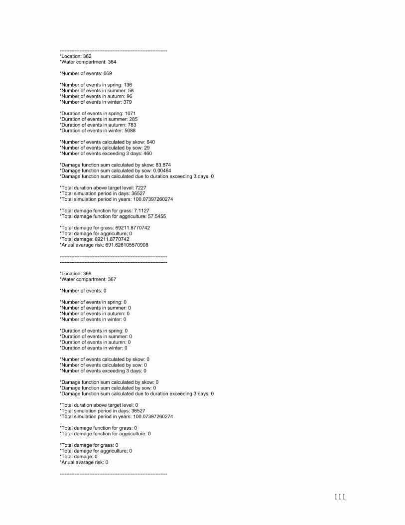
111
----------------------------------------------------------------- *Location: 362 *Water compartment: 364 *Number of events: 669 *Number of events in spring: 136 *Number of events in summer: 58 *Number of events in autumn: 96 *Number of events in winter: 379 *Duration of events in spring: 1071 *Duration of events in summer: 285 *Duration of events in autumn: 783 *Duration of events in winter: 5088 *Number of events calculated by skow: 640 *Number of events calculated by sow: 29 *Number of events exceeding 3 days: 460 *Damage function sum calculated by skow: 83.874 *Damage function sum calculated by sow: 0.00464 *Damage function sum calculated due to duration exceeding 3 days: 0 *Total duration above target level: 7227 *Total simulation period in days: 36527 *Total simulation period in years: 100.07397260274 *Total damage function for grass: 7.1127 *Total damage function for aggriculture: 57.5455 *Total damage for grass: 69211.8770742 *Total damage for aggriculture; 0 *Total damage: 69211.8770742 *Anual avarage risk: 691.626105570908 ----------------------------------------------------------------- ----------------------------------------------------------------- *Location: 369 *Water compartment: 367 *Number of events: 0 *Number of events in spring: 0 *Number of events in summer: 0 *Number of events in autumn: 0 *Number of events in winter: 0 *Duration of events in spring: 0 *Duration of events in summer: 0 *Duration of events in autumn: 0 *Duration of events in winter: 0 *Number of events calculated by skow: 0 *Number of events calculated by sow: 0 *Number of events exceeding 3 days: 0 *Damage function sum calculated by skow: 0 *Damage function sum calculated by sow: 0 *Damage function sum calculated due to duration exceeding 3 days: 0 *Total duration above target level: 0 *Total simulation period in days: 36527 *Total simulation period in years: 100.07397260274 *Total damage function for grass: 0 *Total damage function for aggriculture: 0 *Total damage for grass: 0 *Total damage for aggriculture; 0 *Total damage: 0 *Anual avarage risk: 0 -----------------------------------------------------------------

112
----------------------------------------------------------------- *Location: 370 *Water compartment: 373 *Number of events: 66 *Number of events in spring: 6 *Number of events in summer: 9 *Number of events in autumn: 21 *Number of events in winter: 30 *Duration of events in spring: 11 *Duration of events in summer: 16 *Duration of events in autumn: 33 *Duration of events in winter: 78 *Number of events calculated by skow: 62 *Number of events calculated by sow: 4 *Number of events exceeding 3 days: 4 *Damage function sum calculated by skow: 0.2832 *Damage function sum calculated by sow: 0.00041 *Damage function sum calculated due to duration exceeding 3 days: 0 *Total duration above target level: 138 *Total simulation period in days: 36527 *Total simulation period in years: 100.07397260274 *Total damage function for grass: 0.0472 *Total damage function for aggriculture: 0.2837 *Total damage for grass: 1563.5702808 *Total damage for aggriculture; 6879.5706672 *Total damage: 8443.140948 *Anual avarage risk: 84.3713093692164 ----------------------------------------------------------------- ----------------------------------------------------------------- *Location: 375 *Water compartment: 377 *Number of events: 73 *Number of events in spring: 4 *Number of events in summer: 4 *Number of events in autumn: 17 *Number of events in winter: 48 *Duration of events in spring: 9 *Duration of events in summer: 8 *Duration of events in autumn: 33 *Duration of events in winter: 104 *Number of events calculated by skow: 71 *Number of events calculated by sow: 2 *Number of events exceeding 3 days: 11 *Damage function sum calculated by skow: 2.5919 *Damage function sum calculated by sow: 0.0004 *Damage function sum calculated due to duration exceeding 3 days: 0 *Total duration above target level: 154 *Total simulation period in days: 36527 *Total simulation period in years: 100.07397260274 *Total damage function for grass: 0.0836 *Total damage function for aggriculture: 2.5922 *Total damage for grass: 3194.16372 *Total damage for aggriculture; 96550.3773 *Total damage: 99744.54102 *Anual avarage risk: 996.735406896457 -----------------------------------------------------------------

113
----------------------------------------------------------------- *Location: 381 *Water compartment: 383 *Number of events: 67 *Number of events in spring: 5 *Number of events in summer: 8 *Number of events in autumn: 20 *Number of events in winter: 34 *Duration of events in spring: 10 *Duration of events in summer: 14 *Duration of events in autumn: 33 *Duration of events in winter: 72 *Number of events calculated by skow: 64 *Number of events calculated by sow: 3 *Number of events exceeding 3 days: 5 *Damage function sum calculated by skow: 3.5183 *Damage function sum calculated by sow: 0.00032 *Damage function sum calculated due to duration exceeding 3 days: 0 *Total duration above target level: 129 *Total simulation period in days: 36527 *Total simulation period in years: 100.07397260274 *Total damage function for grass: 0.1396 *Total damage function for aggriculture: 3.4285 *Total damage for grass: 2546.132292 *Total damage for aggriculture; 5558.366484 *Total damage: 8104.498776 *Anual avarage risk: 80.9872981777364 ----------------------------------------------------------------- ----------------------------------------------------------------- *Location: 386 *Water compartment: 385 *Number of events: 623 *Number of events in spring: 157 *Number of events in summer: 65 *Number of events in autumn: 87 *Number of events in winter: 314 *Duration of events in spring: 2320 *Duration of events in summer: 427 *Duration of events in autumn: 1010 *Duration of events in winter: 6578 *Number of events calculated by skow: 597 *Number of events calculated by sow: 26 *Number of events exceeding 3 days: 467 *Damage function sum calculated by skow: 118.5809 *Damage function sum calculated by sow: 0.00448 *Damage function sum calculated due to duration exceeding 3 days: 0 *Total duration above target level: 10335 *Total simulation period in days: 36527 *Total simulation period in years: 100.07397260274 *Total damage function for grass: 14.4597 *Total damage function for aggriculture: 68.9031 *Total damage for grass: 579761.6715 *Total damage for aggriculture; 0 *Total damage: 579761.6715 *Anual avarage risk: 5793.489845521 -----------------------------------------------------------------

114
----------------------------------------------------------------- *Location: 392 *Water compartment: 389 *Number of events: 25 *Number of events in spring: 2 *Number of events in summer: 2 *Number of events in autumn: 5 *Number of events in winter: 16 *Duration of events in spring: 7 *Duration of events in summer: 5 *Duration of events in autumn: 12 *Duration of events in winter: 59 *Number of events calculated by skow: 25 *Number of events calculated by sow: 0 *Number of events exceeding 3 days: 6 *Damage function sum calculated by skow: 0.7509 *Damage function sum calculated by sow: 0 *Damage function sum calculated due to duration exceeding 3 days: 0 *Total duration above target level: 83 *Total simulation period in days: 36527 *Total simulation period in years: 100.07397260274 *Total damage function for grass: 0.02 *Total damage function for aggriculture: 0.751 *Total damage for grass: 519.2802 *Total damage for aggriculture; 24019.971984 *Total damage: 24539.252184 *Anual avarage risk: 245.217846114001 ----------------------------------------------------------------- ----------------------------------------------------------------- *Location: 393 *Water compartment: 395 *Number of events: 266 *Number of events in spring: 17 *Number of events in summer: 17 *Number of events in autumn: 52 *Number of events in winter: 180 *Duration of events in spring: 42 *Duration of events in summer: 35 *Duration of events in autumn: 151 *Duration of events in winter: 451 *Number of events calculated by skow: 262 *Number of events calculated by sow: 4 *Number of events exceeding 3 days: 57 *Damage function sum calculated by skow: 10.6575 *Damage function sum calculated by sow: 0.00041 *Damage function sum calculated due to duration exceeding 3 days: 0 *Total duration above target level: 679 *Total simulation period in days: 36527 *Total simulation period in years: 100.07397260274 *Total damage function for grass: 0.4242 *Total damage function for aggriculture: 9.1666 *Total damage for grass: 10905.1028352 *Total damage for aggriculture; 0 *Total damage: 10905.1028352 *Anual avarage risk: 108.973403461863 -----------------------------------------------------------------

115
----------------------------------------------------------------- *Location: 397 *Water compartment: 399 *Number of events: 210 *Number of events in spring: 15 *Number of events in summer: 22 *Number of events in autumn: 49 *Number of events in winter: 124 *Duration of events in spring: 27 *Duration of events in summer: 34 *Duration of events in autumn: 101 *Duration of events in winter: 231 *Number of events calculated by skow: 210 *Number of events calculated by sow: 0 *Number of events exceeding 3 days: 24 *Damage function sum calculated by skow: 11.5137 *Damage function sum calculated by sow: 0 *Damage function sum calculated due to duration exceeding 3 days: 0 *Total duration above target level: 393 *Total simulation period in days: 36527 *Total simulation period in years: 100.07397260274 *Total damage function for grass: 0.2348 *Total damage function for aggriculture: 11.4786 *Total damage for grass: 10891.3630644 *Total damage for aggriculture; 269281.4820696 *Total damage: 280172.845134 *Anual avarage risk: 2799.73412018589 ----------------------------------------------------------------- ----------------------------------------------------------------- *Location: 403 *Water compartment: 402 *Number of events: 71 *Number of events in spring: 7 *Number of events in summer: 8 *Number of events in autumn: 19 *Number of events in winter: 37 *Duration of events in spring: 12 *Duration of events in summer: 13 *Duration of events in autumn: 29 *Duration of events in winter: 69 *Number of events calculated by skow: 69 *Number of events calculated by sow: 2 *Number of events exceeding 3 days: 4 *Damage function sum calculated by skow: 1.3831 *Damage function sum calculated by sow: 0.00018 *Damage function sum calculated due to duration exceeding 3 days: 0 *Total duration above target level: 123 *Total simulation period in days: 36527 *Total simulation period in years: 100.07397260274 *Total damage function for grass: 0.0957 *Total damage function for aggriculture: 1.3834 *Total damage for grass: 4343.4540765 *Total damage for aggriculture; 3371.124456 *Total damage: 7714.5785325 *Anual avarage risk: 77.0908712797049 -----------------------------------------------------------------

116
----------------------------------------------------------------- *Location: 406 *Water compartment: 407 *Number of events: 1422 *Number of events in spring: 277 *Number of events in summer: 175 *Number of events in autumn: 239 *Number of events in winter: 731 *Duration of events in spring: 816 *Duration of events in summer: 483 *Duration of events in autumn: 966 *Duration of events in winter: 4181 *Number of events calculated by skow: 1392 *Number of events calculated by sow: 30 *Number of events exceeding 3 days: 603 *Damage function sum calculated by skow: 17.938 *Damage function sum calculated by sow: 0.00464 *Damage function sum calculated due to duration exceeding 3 days: 0 *Total duration above target level: 6446 *Total simulation period in days: 36527 *Total simulation period in years: 100.07397260274 *Total damage function for grass: 2.3168 *Total damage function for aggriculture: 17.9429 *Total damage for grass: 109718.076096 *Total damage for aggriculture; 257216.3519688 *Total damage: 366934.4280648 *Anual avarage risk: 3666.73236170542 ----------------------------------------------------------------- ----------------------------------------------------------------- *Location: 409 *Water compartment: 411 *Number of events: 1553 *Number of events in spring: 337 *Number of events in summer: 215 *Number of events in autumn: 248 *Number of events in winter: 753 *Duration of events in spring: 1178 *Duration of events in summer: 645 *Duration of events in autumn: 1186 *Duration of events in winter: 5213 *Number of events calculated by skow: 1529 *Number of events calculated by sow: 24 *Number of events exceeding 3 days: 746 *Damage function sum calculated by skow: 23.9591 *Damage function sum calculated by sow: 0.00347 *Damage function sum calculated due to duration exceeding 3 days: 0 *Total duration above target level: 8222 *Total simulation period in days: 36527 *Total simulation period in years: 100.07397260274 *Total damage function for grass: 3.1277 *Total damage function for aggriculture: 23.9624 *Total damage for grass: 154210.873176 *Total damage for aggriculture; 643520.4120576 *Total damage: 797731.2852336 *Anual avarage risk: 7971.63442781208 -----------------------------------------------------------------

117
----------------------------------------------------------------- *Location: 415 *Water compartment: 414 *Number of events: 288 *Number of events in spring: 29 *Number of events in summer: 8 *Number of events in autumn: 35 *Number of events in winter: 216 *Duration of events in spring: 188 *Duration of events in summer: 39 *Duration of events in autumn: 269 *Duration of events in winter: 1827 *Number of events calculated by skow: 288 *Number of events calculated by sow: 0 *Number of events exceeding 3 days: 187 *Damage function sum calculated by skow: 27.0971 *Damage function sum calculated by sow: 0 *Damage function sum calculated due to duration exceeding 3 days: 0 *Total duration above target level: 2323 *Total simulation period in days: 36527 *Total simulation period in years: 100.07397260274 *Total damage function for grass: 0.9778 *Total damage function for aggriculture: 23.8066 *Total damage for grass: 27980.67591 *Total damage for aggriculture; 0 *Total damage: 27980.67591 *Anual avarage risk: 279.607586572578 ----------------------------------------------------------------- ----------------------------------------------------------------- *Location: 418 *Water compartment: 419 *Number of events: 1394 *Number of events in spring: 343 *Number of events in summer: 183 *Number of events in autumn: 236 *Number of events in winter: 632 *Duration of events in spring: 1532 *Duration of events in summer: 570 *Duration of events in autumn: 1175 *Duration of events in winter: 6852 *Number of events calculated by skow: 1394 *Number of events calculated by sow: 0 *Number of events exceeding 3 days: 765 *Damage function sum calculated by skow: 16.869 *Damage function sum calculated by sow: 0 *Damage function sum calculated due to duration exceeding 3 days: 0 *Total duration above target level: 10129 *Total simulation period in days: 36527 *Total simulation period in years: 100.07397260274 *Total damage function for grass: 1.5844 *Total damage function for aggriculture: 16.8681 *Total damage for grass: 41173.4399724 *Total damage for aggriculture; 0 *Total damage: 41173.4399724 *Anual avarage risk: 411.441318237037 -----------------------------------------------------------------

118
----------------------------------------------------------------- *Location: 424 *Water compartment: 423 *Number of events: 37 *Number of events in spring: 2 *Number of events in summer: 4 *Number of events in autumn: 10 *Number of events in winter: 21 *Duration of events in spring: 7 *Duration of events in summer: 8 *Duration of events in autumn: 18 *Duration of events in winter: 71 *Number of events calculated by skow: 37 *Number of events calculated by sow: 0 *Number of events exceeding 3 days: 6 *Damage function sum calculated by skow: 3.9782 *Damage function sum calculated by sow: 0 *Damage function sum calculated due to duration exceeding 3 days: 0 *Total duration above target level: 104 *Total simulation period in days: 36527 *Total simulation period in years: 100.07397260274 *Total damage function for grass: 0.071 *Total damage function for aggriculture: 3.4962 *Total damage for grass: 2568.30075 *Total damage for aggriculture; 44146.5174 *Total damage: 46714.81815 *Anual avarage risk: 466.815655279801 ----------------------------------------------------------------- ----------------------------------------------------------------- *Location: 425 *Water compartment: 427 *Number of events: 9 *Number of events in spring: 1 *Number of events in summer: 2 *Number of events in autumn: 2 *Number of events in winter: 4 *Duration of events in spring: 1 *Duration of events in summer: 2 *Duration of events in autumn: 4 *Duration of events in winter: 8 *Number of events calculated by skow: 9 *Number of events calculated by sow: 0 *Number of events exceeding 3 days: 0 *Damage function sum calculated by skow: 0.885 *Damage function sum calculated by sow: 0 *Damage function sum calculated due to duration exceeding 3 days: 0 *Total duration above target level: 15 *Total simulation period in days: 36527 *Total simulation period in years: 100.07397260274 *Total damage function for grass: 0.0089 *Total damage function for aggriculture: 0.885 *Total damage for grass: 512.7221025 *Total damage for aggriculture; 9897.309 *Total damage: 10410.0311025 *Anual avarage risk: 104.026210162966 -----------------------------------------------------------------

119
----------------------------------------------------------------- *Location: 431 *Water compartment: 430 *Number of events: 0 *Number of events in spring: 0 *Number of events in summer: 0 *Number of events in autumn: 0 *Number of events in winter: 0 *Duration of events in spring: 0 *Duration of events in summer: 0 *Duration of events in autumn: 0 *Duration of events in winter: 0 *Number of events calculated by skow: 0 *Number of events calculated by sow: 0 *Number of events exceeding 3 days: 0 *Damage function sum calculated by skow: 0 *Damage function sum calculated by sow: 0 *Damage function sum calculated due to duration exceeding 3 days: 0 *Total duration above target level: 0 *Total simulation period in days: 36527 *Total simulation period in years: 100.07397260274 *Total damage function for grass: 0 *Total damage function for aggriculture: 0 *Total damage for grass: 0 *Total damage for aggriculture; 0 *Total damage: 0 *Anual avarage risk: 0 ----------------------------------------------------------------- ----------------------------------------------------------------- *Location: 432 *Water compartment: 434 *Number of events: 1062 *Number of events in spring: 155 *Number of events in summer: 122 *Number of events in autumn: 176 *Number of events in winter: 609 *Duration of events in spring: 451 *Duration of events in summer: 322 *Duration of events in autumn: 690 *Duration of events in winter: 39359 *Number of events calculated by skow: 1062 *Number of events calculated by sow: 0 *Number of events exceeding 3 days: 420 *Damage function sum calculated by skow: 100.6387 *Damage function sum calculated by sow: 0 *Damage function sum calculated due to duration exceeding 3 days: 0 *Total duration above target level: 40822 *Total simulation period in days: 36527 *Total simulation period in years: 100.07397260274 *Total damage function for grass: 2.4686 *Total damage function for aggriculture: 70.5741 *Total damage for grass: 193104.4872312 *Total damage for aggriculture; 0 *Total damage: 193104.4872312 *Anual avarage risk: 1929.67031263724 -----------------------------------------------------------------

120
5-Statistical information on elevation data of water compartments Comp. Count Area Min Max Range Mean Std Variety Majority Minority Median
306 1939.00 1211875 -648.00 -161.00 487.00 -475.83 61.07 307.00 -486.00 -648.00 -481.00312 1280.00 800000 -604.00 -355.00 249.00 -486.00 31.97 175.00 -481.00 -604.00 -485.00317 1331.00 831875 -678.00 487.00 1165.00 -465.92 88.22 261.00 -481.00 -678.00 -483.00322 1253.00 783125 -609.00 -412.00 197.00 -508.63 19.41 106.00 -504.00 -609.00 -509.00325 1506.00 941250 -674.00 1627.00 2301.00 -249.67 281.77 689.00 -482.00 -674.00 -344.00330 900.00 562500 -626.00 1583.00 2209.00 -232.96 318.33 572.00 -505.00 -626.00 -315.00336 427.00 266875 -618.00 603.00 1221.00 -352.23 232.97 254.00 -507.00 -618.00 -459.00337 754.00 471250 -607.00 676.00 1283.00 -397.36 184.11 300.00 -493.00 -607.00 -483.00344 1142.00 713750 -619.00 -155.00 464.00 -474.10 74.43 253.00 -486.00 -619.00 -496.00346 1780.00 1112500 -629.00 657.00 1286.00 -422.29 128.55 420.00 -518.00 -629.00 -468.00352 922.00 576250 -598.00 993.00 1591.00 -132.09 268.27 373.00 -239.00 -598.00 -223.00359 441.00 275625 -494.00 816.00 1310.00 -100.61 228.14 266.00 -233.00 -494.00 -206.00364 285.00 178125 -496.00 -105.00 391.00 -248.87 47.97 125.00 -256.00 -496.00 -242.00367 409.00 255625 -603.00 1631.00 2234.00 -123.63 357.03 324.00 -472.00 -603.00 -238.00373 1301.00 813125 -651.00 1631.00 2282.00 -410.18 212.44 437.00 -508.00 -651.00 -491.00377 1033.00 645625 -646.00 45.00 691.00 -486.85 89.65 276.00 -528.00 -646.00 -516.00383 649.00 405625 -620.00 895.00 1515.00 -376.16 202.04 262.00 -452.00 -620.00 -447.00385 786.00 491250 -597.00 -295.00 302.00 -478.38 35.07 152.00 -472.00 -597.00 -480.00389 810.00 506250 -638.00 287.00 925.00 -444.25 81.63 260.00 -450.00 -638.00 -460.00395 524.00 327500 -576.00 -192.00 384.00 -451.44 66.70 181.00 -490.00 -576.00 -474.00399 1298.00 811250 -595.00 -190.00 405.00 -452.99 49.76 225.00 -487.00 -595.00 -465.00402 1048.00 655000 -585.00 -192.00 393.00 -417.80 69.13 269.00 -468.00 -585.00 -439.00407 1358.00 848750 -553.00 -142.00 411.00 -270.12 48.10 220.00 -283.00 -553.00 -264.00411 1591.00 994375 -588.00 -111.00 477.00 -249.80 46.30 220.00 -233.00 -588.00 -242.00414 553.00 345625 -581.00 -26.00 555.00 -451.30 94.10 215.00 -514.00 -581.00 -489.00419 638.00 398750 -495.00 55.00 550.00 -267.85 75.20 194.00 -291.00 -495.00 -286.00423 898.00 561250 -625.00 -191.00 434.00 -479.97 73.64 237.00 -530.00 -613.00 -504.00427 1243.00 776875 -629.00 -175.00 454.00 -478.97 69.17 267.00 -525.00 -629.00 -504.00430 1528.00 955000 -636.00 -171.00 465.00 -499.36 63.62 270.00 -523.00 -636.00 -517.00434 1569.00 980625 -598.00 -194.00 404.00 -471.10 52.74 249.00 -478.00 -598.00 -477.00

121
Top Related