


Languages
Pages
Legal


RICE UNIVERSITY
Array Optimizations for High Productivity
Programming Languagesby
Mackale Joyner
A Thesis Submittedin Partial Fulfillment of theRequirements for the Degree
Doctor of PhilosophyApproved, Thesis Committee:
Vivek Sarkar , Co-ChairE.D. Butcher Professor of ComputerScience
Zoran Budimlic, Co-ChairResearch Scientist
Keith CooperL. John and Ann H. Doerr Professor ofComputer Engineering
John Mellor-CrummeyProfessor of Computer Science
Richard TapiaUniversity ProfessorMaxfield-Oshman Professor inEngineering
Houston, Texas
September, 2008

ABSTRACT
Array Optimizations for High Productivity ProgrammingLanguages
by
Mackale Joyner
While the HPCS languages (Chapel, Fortress and X10) have introduced improve-
ments in programmer productivity, several challenges still remain in delivering high
performance. In the absence of optimization, the high-level language constructs that
improve productivity can result in order-of-magnitude runtime performance degrada-
tions.
This dissertation addresses the problem of efficient code generation for high-level
array accesses in the X10 language. The X10 language supports rank-independent
specification of loop and array computations using regions and points. Three as-
pects of high-level array accesses in X10 are important for productivity but also pose
significant performance challenges: high-level accesses are performed through Point
objects rather than integer indices, variables containing references to arrays are rank-
independent, and array subscripts are verified as legal array indices during runtime
program execution.
Our solution to the first challenge is to introduce new analyses and transforma-
tions that enable automatic inlining and scalar replacement of Point objects. Our
solution to the second challenge is a hybrid approach. We use an interprocedural
rank analysis algorithm to automatically infer ranks of arrays in X10. We use rank
analysis information to enable storage transformations on arrays. If rank-independent

array references still remain after compiler analysis, the programmer can use X10’s
dependent type system to safely annotate array variable declarations with additional
information for the rank and region of the variable, and to enable the compiler to gen-
erate efficient code in cases where the dependent type information is available. Our
solution to the third challenge is to use a new interprocedural array bounds analysis
approach using regions to automatically determine when runtime bounds checks are
not needed.
Our performance results show that our optimizations deliver performance that
rivals the performance of hand-tuned code with explicit rank-specific loops and lower-
level array accesses, and is up to two orders of magnitude faster than unoptimized,
high-level X10 programs. These optimizations also result in scalability improvements
of X10 programs as we increase the number of CPUs. While we perform the opti-
mizations primarily in X10, these techniques are applicable to other high-productivity
languages such as Chapel and Fortress.

Acknowledgments
I would first like to thank God for giving me the diligence and perseverance to endure
the long PhD journey. Only by His grace was I able to complete the degree require-
ments. There are many people who I am grateful to for helping me along the way
to obtaining the PhD. I would like to thank my thesis co-chairs Zoran Budimlic and
Vivek Sarkar for their invaluable research advice and their tireless efforts to ensure
that I would successfully defend my thesis. I am deeply indebted to them. I would
like to thank the rest of my thesis committee: Keith Cooper, John Mellor-Crummey,
and Richard Tapia. In addition to research or career advice, each has helped to fi-
nancially support me (along with my advisors) during graduate school with grants
and fellowships which I am truly grateful for. Before I go any further, I certainly
must acknowledge my other advisor, the late Ken Kennedy. It is because of him
that I even had the opportunity to attend graduate school at Rice. Technical advice
only scratches the surface of what he gave me. I am forever grateful for the many
doors that he opened for me from the very beginning of my graduate school career.
There are lots of others at Rice that helped me navigate the sometimes rough waters
of graduate school in their own ways. The non-exhaustive list includes Raj Barik,
Theresa Chatman, Cristi Coarfa, Yuri Dotsenko, Jason Eckhardt, Nathan Froyd,
John Garvin, Tim Harvey, Chuck Koelbel, Gabriel Marin, Cheryl McCosh, Apan
Qasem, Jun Shirako, Todd Waterman, and Rui Zhang.
I was also privileged to work with several industry partners during my graduate
school career who went out of their way to help further my research efforts. These
include Eric Allen (Sun), Brad Chamberlain (Cray), Steve Deitz (Cray), Chris Don-
awa (IBM), Allan Kielstra (IBM), Igor Peshansky (IBM), Vijay Saraswat (IBM), and

v
Sharon Selzo (IBM). I would also like to thank both IBM and Waseda University for
providing access to their machines. In addition to research advice, I also have been
fortunate to receive outstanding mentoring advice thanks to Juan Gilbert (Auburn)
and the Rice AGEP program led by Richard Tapia with vital support from Enrique
Barrera, Bonnie Bartel, Theresa Chatman, and Illya Hicks.
Last but not least, I would like to thank my very strong family support system.
These include my best friend Andrew who has always been like a brother to me, my
in-laws who unconditionally support me, my aunt Sharon who has for my entire life
gone out of her way to help me, my mom who sacrificed part of her life for me and
believes in me more than I do at times, and my wife who has deeply shown her love
and support for me as I worked hard to finish my degree and who is probably looking
forward to reintroducing me to the stove and the washing machine now that the final
push to complete the PhD is over. I am truly blessed.

Contents
Abstract ii
Acknowledgments iv
List of Illustrations ix
List of Tables xvi
1 Introduction 1
2 Background 4
2.1 Message Passing Interface . . . . . . . . . . . . . . . . . . . . . . . . 4
2.2 Data-Parallel Languages . . . . . . . . . . . . . . . . . . . . . . . . . 5
2.2.1 High Performance Fortran . . . . . . . . . . . . . . . . . . . . 5
2.2.2 ZPL . . . . . . . . . . . . . . . . . . . . . . . . . . . . . . . . 6
2.2.3 CM Fortran . . . . . . . . . . . . . . . . . . . . . . . . . . . . 6
2.3 Task-Parallel Languages . . . . . . . . . . . . . . . . . . . . . . . . . 7
2.3.1 OpenMP . . . . . . . . . . . . . . . . . . . . . . . . . . . . . . 7
2.3.2 Java . . . . . . . . . . . . . . . . . . . . . . . . . . . . . . . . 7
2.4 Partitioned Global Address Space Languages . . . . . . . . . . . . . . 8
2.4.1 Titanium . . . . . . . . . . . . . . . . . . . . . . . . . . . . . 8
2.4.2 Unified Parallel C . . . . . . . . . . . . . . . . . . . . . . . . . 9
2.4.3 Co-Array Fortran . . . . . . . . . . . . . . . . . . . . . . . . . 9
2.5 High Productivity Computing Languages . . . . . . . . . . . . . . . . 10
2.5.1 X10 . . . . . . . . . . . . . . . . . . . . . . . . . . . . . . . . 10
2.5.2 Chapel . . . . . . . . . . . . . . . . . . . . . . . . . . . . . . . 11
2.5.3 Fortress . . . . . . . . . . . . . . . . . . . . . . . . . . . . . . 12

vii
3 Related Work 14
3.1 High-Level Iteration . . . . . . . . . . . . . . . . . . . . . . . . . . . 14
3.1.1 CLU . . . . . . . . . . . . . . . . . . . . . . . . . . . . . . . . 14
3.1.2 Sather . . . . . . . . . . . . . . . . . . . . . . . . . . . . . . . 15
3.1.3 Coroutine . . . . . . . . . . . . . . . . . . . . . . . . . . . . . 15
3.1.4 C++, Java, and Python . . . . . . . . . . . . . . . . . . . . . 15
3.1.5 Sisal and Titanium . . . . . . . . . . . . . . . . . . . . . . . . 16
3.2 Optimized Compilation of Object-Oriented Languages . . . . . . . . . 16
3.2.1 Object Inlining . . . . . . . . . . . . . . . . . . . . . . . . . . 16
3.2.2 Semantic Inlining . . . . . . . . . . . . . . . . . . . . . . . . . 17
3.2.3 Point Inlining in Titanium . . . . . . . . . . . . . . . . . . . . 17
3.2.4 Optimizing Array Accesses . . . . . . . . . . . . . . . . . . . . 18
3.2.5 Type Inference . . . . . . . . . . . . . . . . . . . . . . . . . . 20
4 Efficient High-Level X10 Array Computations 23
4.1 X10 Language Overview . . . . . . . . . . . . . . . . . . . . . . . . . 26
4.2 Improving the Performance of X10 Language Abstractions . . . . . . 31
4.3 Point Inlining Algorithm . . . . . . . . . . . . . . . . . . . . . . . . . 32
4.4 Use of Dependent Type Information for Improved Code Generation . 36
4.5 X10 General Array Conversion . . . . . . . . . . . . . . . . . . . . . . 38
4.6 Rank Analysis . . . . . . . . . . . . . . . . . . . . . . . . . . . . . . . 38
4.7 Safety Analysis . . . . . . . . . . . . . . . . . . . . . . . . . . . . . . 42
4.8 Extensions for Increased Precision . . . . . . . . . . . . . . . . . . . . 43
4.9 Array Transformation . . . . . . . . . . . . . . . . . . . . . . . . . . . 47
4.10 Object Inlining in Fortress . . . . . . . . . . . . . . . . . . . . . . . . 47
5 Eliminating Array Bounds Checks with X10 Regions 49
5.1 Intraprocedural Region Analysis . . . . . . . . . . . . . . . . . . . . . 55
5.2 Interprocedural Region Analysis . . . . . . . . . . . . . . . . . . . . . 58

viii
5.3 Region Algebra . . . . . . . . . . . . . . . . . . . . . . . . . . . . . . 66
5.4 Improving Productivity with Array Views . . . . . . . . . . . . . . . 68
5.5 Interprocedural Linearized Array Bounds Analysis . . . . . . . . . . . 77
6 High Productivity Language Iteration 82
6.1 Overview of Chapel . . . . . . . . . . . . . . . . . . . . . . . . . . . . 84
6.2 Chapel Iterators . . . . . . . . . . . . . . . . . . . . . . . . . . . . . . 85
6.3 Invoking Multiple Iterators . . . . . . . . . . . . . . . . . . . . . . . . 90
6.4 Implementation Techniques . . . . . . . . . . . . . . . . . . . . . . . 91
6.4.1 Sequence Implementation . . . . . . . . . . . . . . . . . . . . 91
6.4.2 Nested Function Implementation . . . . . . . . . . . . . . . . 93
6.5 Zippered Iteration . . . . . . . . . . . . . . . . . . . . . . . . . . . . . 95
7 Performance Results 101
8 Conclusions and Future Work 118
Bibliography 121

Illustrations
4.1 X10 compiler structure . . . . . . . . . . . . . . . . . . . . . . . . . . 24
4.2 Region operations in X10 . . . . . . . . . . . . . . . . . . . . . . . . . 28
4.3 Java Grande SOR benchmark . . . . . . . . . . . . . . . . . . . . . . 30
4.4 X10 source code of loop example adapted from the Java Grande
sparsematmult benchmark . . . . . . . . . . . . . . . . . . . . . . . . 32
4.5 Source code of loop following translation from unoptimized X10 to
Java by X10 compiler . . . . . . . . . . . . . . . . . . . . . . . . . . . 32
4.6 X10 source code following optimization of X10 loop body . . . . . . . 33
4.7 Source code of loop following translation of optimized X10 to Java by
X10 compiler . . . . . . . . . . . . . . . . . . . . . . . . . . . . . . . 33
4.8 Rank Analysis Algorithm . . . . . . . . . . . . . . . . . . . . . . . . . 34
4.9 Algorithm for X10 point inlining . . . . . . . . . . . . . . . . . . . . . 35
4.10 X10 for loop example from Figure 4.4, extended with dependent type
declarations . . . . . . . . . . . . . . . . . . . . . . . . . . . . . . . . 36
4.11 Source code for loop body translated from X10 to Java by X10 compiler 37
4.12 Type lattice for ranks . . . . . . . . . . . . . . . . . . . . . . . . . . . 40
4.13 X10 code fragment adapted from JavaGrande X10 montecarlo
benchmarks showing when our rank inference algorithm needs to
propagate rank information left to right. . . . . . . . . . . . . . . . . 41
4.14 X10 code fragment adapted from JavaGrande X10 montecarlo
benchmarks showing when our safety inference algorithm needs to
propagate rank information left to right. . . . . . . . . . . . . . . . . 44

x
4.15 Safety Analysis Algorithm . . . . . . . . . . . . . . . . . . . . . . . . 45
5.1 Example displaying both the code source view and analysis view. We
designed the analysis view to aid region analysis in discovering array
region and value range relationships by simplifying the source view. . 56
5.2 X10 region analysis compiler framework . . . . . . . . . . . . . . . . . 57
5.3 Java Grande Sparse Matrix Multiplication kernel (source view). . . . 59
5.4 Java Grande Sparse Matrix Multiplication kernel (analysis view). . . 60
5.5 Type lattice for region equivalence . . . . . . . . . . . . . . . . . . . . 61
5.6 Intraprocedural region analysis algorithm builds local region
relationships. . . . . . . . . . . . . . . . . . . . . . . . . . . . . . . . 62
5.7 Type lattice for sub-region relation . . . . . . . . . . . . . . . . . . . 64
5.8 Interprocedural region analysis algorithm maps variables of type X10
array, point, and region to a concrete region. . . . . . . . . . . . . . . 67
5.9 Java Grande LU factorization kernel. . . . . . . . . . . . . . . . . . . 69
5.10 Region algebra algorithm discovers integers and points that have a
region association. . . . . . . . . . . . . . . . . . . . . . . . . . . . . 70
5.11 Hexahedral cells code showing the initialization of multi-dimensional
arrays x, y, and z. . . . . . . . . . . . . . . . . . . . . . . . . . . . . . 72
5.12 Hexahedral cells code showing that problems arise when representing
arrays x, y, and z as 3-dimensional arrays due to programmers
indexing into these arrays using an array access returning integer
value instead of a triplet. . . . . . . . . . . . . . . . . . . . . . . . . . 73
5.13 Array views xv, yv, and zv enable the programmer to productivity
implement 3-dimensional array computations inside the innermost loop. 74

xi
5.14 We highlight the array transformation of X10 arrays into Java arrays
to boost runtime performance. In this hexahedral cells volume
calculation code fragment, our compiler could not transform X10
arrays x, y, z, xv, yv, zv into Java arrays because the Java language
doesn’t have an equivalent array view operation. . . . . . . . . . . . . 75
5.15 We illustrate the array transformation of X10 arrays into Java arrays
and subsequent Java array linearization. Note that LinearViewAuto
is a method our compiler automatically inserts to linearize a
multi-dimensional X10 array and LinearViewHand is a method the
programmer inserts to linearize an X10 region. . . . . . . . . . . . . . 76
5.16 We show the final version for the Hexahedral cells code which
demonstrates the compiler’s ability to translate X10 arrays into Java
arrays in the presence of array views. . . . . . . . . . . . . . . . . . . 78
5.17 Array u is a 3-dimensional array that the programmer has linearized
to improve runtime performance. Converting the linearized array into
an X10 3-dimensional array would remove the the complex array
subscript expression inside the loop in zero3’s method body and
enable bounds analysis to attempt to discover a superfluous bounds
check. However, this example shows it may not be possible to always
perform the conversion. . . . . . . . . . . . . . . . . . . . . . . . . . . 80
5.18 This MG code fragment shows an opportunity to remove all array r
bounds checks inside the psinv method because those checks are all
redundant since the programmer must invoke method zero3 prior to
method psinv. . . . . . . . . . . . . . . . . . . . . . . . . . . . . . . . 81
6.1 A basic iterator example showing how Chapel iterators separate the
specification of an iteration from the actual computation. . . . . . . . 87

xii
6.2 A parallel excerpt from the Smith-Waterman algorithm written in
Chapel using iterators. The ordered keyword is used to respect the
sequential constraints within the loop body. . . . . . . . . . . . . . . 88
6.3 An iterator example showing how to use Chapel iterators to traverse
an abstract syntax tree (AST). . . . . . . . . . . . . . . . . . . . . . 89
6.4 An implementation of tiled iteration using the sequence-based approach. 92
6.5 An implementation of tiled iteration using the nested function-based
approach. . . . . . . . . . . . . . . . . . . . . . . . . . . . . . . . . . 94
6.6 An example of zippered iteration in Chapel. . . . . . . . . . . . . . . 96
6.7 An implementation of zippered iteration using state variables. . . . . 99
6.8 A multi-threaded implementation of zippered iteration using sync
variables. . . . . . . . . . . . . . . . . . . . . . . . . . . . . . . . . . 100
7.1 Comparison of the optimized sequential X10 benchmarks relative to
the X10 light baseline . . . . . . . . . . . . . . . . . . . . . . . . . . . 104
7.2 Relative Scalability of Optimized and Unoptimized X10 versions of
the sparsematmult benchmark with initial minimum heap size of 2
GB (and maximum heap size of 2GB). The Optimized speedup is
relative to the 1-CPU optimized performance, and the Unoptimized
speedup is relative to the 1-CPU unoptimized performance. . . . . . . 106
7.3 Scalability of Optimized and Unoptimized X10 versions of the
sparsematmult benchmark with initial minimum heap size of of 4 MB
(and maximum heap size of 2GB). The Optimized speedup is relative
to the 1-CPU optimized performance, and the Unoptimized speedup
is relative to the 1-CPU unoptimized performance. . . . . . . . . . . . 106

xiii
7.4 Relative Scalability of Optimized and Unoptimized X10 versions of
the lufact benchmark with initial minimum heap size of 2 GB (and
maximum heap size of 2GB). The Optimized speedup is relative to
the 1-CPU optimized performance, and the Unoptimized speedup is
relative to the 1-CPU unoptimized performance. . . . . . . . . . . . . 107
7.5 Scalability of Optimized and Unoptimized X10 versions of the lufact
benchmark with initial minimum heap size of of 4 MB (and
maximum heap size of 2GB). The Optimized speedup is relative to
the 1-CPU optimized performance, and the Unoptimized speedup is
relative to the 1-CPU unoptimized performance. . . . . . . . . . . . . 107
7.6 Relative Scalability of Optimized and Unoptimized X10 versions of
the sor benchmark with initial minimum heap size of 2 GB (and
maximum heap size of 2GB). The Optimized speedup is relative to
the 1-CPU optimized performance, and the Unoptimized speedup is
relative to the 1-CPU unoptimized performance. . . . . . . . . . . . . 108
7.7 Scalability of Optimized and Unoptimized X10 versions of the sor
benchmark with initial minimum heap size of of 4 MB (and
maximum heap size of 2GB). The Optimized speedup is relative to
the 1-CPU optimized performance, and the Unoptimized speedup is
relative to the 1-CPU unoptimized performance. . . . . . . . . . . . . 108
7.8 Relative Scalability of Optimized and Unoptimized X10 versions of
the series benchmark with initial minimum heap size of 2 GB (and
maximum heap size of 2GB). The Optimized speedup is relative to
the 1-CPU optimized performance, and the Unoptimized speedup is
relative to the 1-CPU unoptimized performance. . . . . . . . . . . . . 109

xiv
7.9 Scalability of Optimized and Unoptimized X10 versions of the series
benchmark with initial minimum heap size of of 4 MB (and
maximum heap size of 2GB). The Optimized speedup is relative to
the 1-CPU optimized performance, and the Unoptimized speedup is
relative to the 1-CPU unoptimized performance. . . . . . . . . . . . . 109
7.10 Relative Scalability of Optimized and Unoptimized X10 versions of
the crypt benchmark with initial minimum heap size of 2 GB (and
maximum heap size of 2GB). The Optimized speedup is relative to
the 1-CPU optimized performance, and the Unoptimized speedup is
relative to the 1-CPU unoptimized performance. . . . . . . . . . . . . 110
7.11 Relative Scalability of Optimized and Unoptimized X10 versions of
the montecarlo benchmark with initial minimum heap size of 2 GB
(and maximum heap size of 2GB). The Optimized speedup is relative
to the 1-CPU optimized performance, and the Unoptimized speedup
is relative to the 1-CPU unoptimized performance. . . . . . . . . . . . 110
7.12 Relative Scalability of Optimized and Unoptimized X10 versions of
the moldyn benchmark with initial minimum heap size of 2 GB (and
maximum heap size of 2GB). The Optimized speedup is relative to
the 1-CPU optimized performance, and the Unoptimized speedup is
relative to the 1-CPU unoptimized performance. . . . . . . . . . . . . 111
7.13 Relative Scalability of Optimized and Unoptimized X10 versions of
the raytracer benchmark with initial minimum heap size of 2 GB
(and maximum heap size of 2GB). The Optimized speedup is relative
to the 1-CPU optimized performance, and the Unoptimized speedup
is relative to the 1-CPU unoptimized performance. . . . . . . . . . . . 111
7.14 Speedup of Optimized X10 version relative to Unoptimized X10 version.112
7.15 Speedup of Optimized X10 version relative to Unoptimized X10
version (zoom in of Figure 7.14). . . . . . . . . . . . . . . . . . . . . . 113

xv
7.16 Comparison of the X10 light baseline to the optimized sequential X10
benchmarks with compiler inserted annotations used to signal the
VM when to eliminate bounds checks. . . . . . . . . . . . . . . . . . . 116
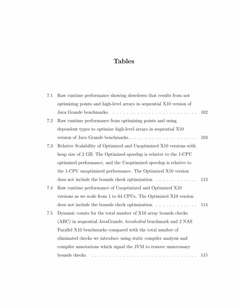
Tables
7.1 Raw runtime performance showing slowdown that results from not
optimizing points and high-level arrays in sequential X10 version of
Java Grande benchmarks. . . . . . . . . . . . . . . . . . . . . . . . . 102
7.2 Raw runtime performance from optimizing points and using
dependent types to optimize high-level arrays in sequential X10
version of Java Grande benchmarks. . . . . . . . . . . . . . . . . . . . 103
7.3 Relative Scalability of Optimized and Unoptimized X10 versions with
heap size of 2 GB. The Optimized speedup is relative to the 1-CPU
optimized performance, and the Unoptimized speedup is relative to
the 1-CPU unoptimized performance. The Optimized X10 version
does not include the bounds check optimization. . . . . . . . . . . . . 113
7.4 Raw runtime performance of Unoptimized and Optimized X10
versions as we scale from 1 to 64 CPUs. The Optimized X10 version
does not include the bounds check optimization. . . . . . . . . . . . . 114
7.5 Dynamic counts for the total number of X10 array bounds checks
(ABC) in sequential JavaGrande, hexahedral benchmark and 2 NAS
Parallel X10 benchmarks compared with the total number of
eliminated checks we introduce using static compiler analysis and
compiler annotations which signal the JVM to remove unnecessary
bounds checks. . . . . . . . . . . . . . . . . . . . . . . . . . . . . . . 115

xvii
7.6 Raw sequential runtime performance of JavaGrande and 2 NAS
Parallel X10 benchmarks with static compiler analysis to signal the
JVM to eliminate unnecessary array bounds checks. These results
were obtained on the IBM 16-way SMP because the J9 VM has the
special option to eliminate individual bounds checks when directed by
the compiler. . . . . . . . . . . . . . . . . . . . . . . . . . . . . . . . 117
7.7 Fortran, Unoptimized X10, Optimized X10, and Java raw sequential
runtime performance comparison (in seconds) for 2 NAS Parallel
benchmarks (cg, mg). These results were obtained on the IBM
16-way SMP machine. . . . . . . . . . . . . . . . . . . . . . . . . . . 117

1
Chapter 1
Introduction
Chapel, Fortress and X10, the three languages initially developed within DARPA’s
High-Productivity Computing System (HPCS) program, are all parallel high-level
object-oriented languages designed to deliver both high-productivity and high per-
formance. These languages offer abstractions that enable programmers to develop
efficient scientific applications for parallel environments without having to explicitly
manage many of the details encountered in low level parallel programming. These
languages’ abstractions provide the mechanisms necessary to improve productivity in
high-performance scientific computing. Unfortunately, runtime performance usually
suffers when programmers use early implementations of these languages. Compiler
optimizations are crucial to reducing performance penalties resulting from their ab-
stractions. By reducing, or in some cases eliminating the performance penalties,
these compiler optimizations should facilitate future adoption of high-productivity
languages for high-performance computing by the broad scientific community.
This dissertation focuses on developing productive and efficient implementations of
high-level array operations and loop iteration constructs for high-productivity parallel
languages. Arrays are important because they are a principal data structure used in
scientific applications. Loops are important because they are the primary control
structure in scientific applications and they tend to dominate execution time. Our
compiler enhancements are designed for high-productivity languages in general and
are applicable to all three HPCS languages. This dissertation reports our work on
optimizing array accesses in X10 (Chapters 4 and 5) and implementing loop iterators
in Chapel (Chapter 6). We take advantage of language features to develop the object

2
inlining work in part in Fortress (Chapter 4), enabling us to make contributions to all
three high-productivity languages. While we detail each contribution in the context
of a specific HPCS language as a proof of concept, we want to emphasize that each
contribution will be applicable to other high-productivity languages as well.
This work addresses several productivity and performance issues related to high-
level loop iteration and array operations. We begin by discussing high-level array
accesses. We develop a variant of the object inlining compiler transformation to
produce efficient representations for points. A point object identifies an element in a
region, and can be used as a multi-dimensional loop index as well as an index into
a multi-dimensional array. Object inlining is a transformation designed to replace
an object by its inlined fields, resulting in direct field accesses and elimination of
the object’s allocation and memory costs. We employ a variant of type analysis to
discover the dimensionality of points before applying this transformation. We extend
object inlining to handle all final object types in scientific computing. We also detail
a transformation to generate an efficient array implementation for high-level arrays
in high-productivity languages. We evaluate the array transformation that converts
high-level multidimensional X10 arrays into lower-level multidimensional Java arrays,
when legal to do so. In addition, this thesis makes important advancements to the
array bounds analysis problem. We highlight the importance of high-level language
abstractions which help our compilation techniques discover and report superfluous
bounds checks to the Java Virtual Machine.
We then turn our attention to iterator implementation. An iterator is a control
construct that encapsulates the manner in which a data structure is traversed. We
illustrate why iterators are important for productive application development and we
demonstrate how to efficiently implement iterators in a high-productivity language.
While most of our contributions target single-thread performance, we demonstrate
the impact that our optimizations have on parallel performance. In particular, this
thesis illustrates the effect these transformations have on scalability as we increase

3
the number of CPUs.
This research highlights the advantages of providing abstractions for iterating over
data structures in a productive manner. It addresses both implementation details and
optimization opportunities to leverage support for these abstractions in a scientific
computing environment. The dissertation presents experimental results that demon-
strate the importance of this work. Subsequent discussion summarizes our results
and provides insight into possible future extensions of this research.
Thesis Statement: Although runtime performance has suffered in the past when
scientists used high productivity languages with high-level array accesses, our thesis
is that these overheads can be mitigated by compiler optimizations, thereby enabling
scientists to develop code with both high productivity and high performance. The
optimizations introduced in this dissertation for high-level array accesses in X10 result
in performance that rivals the performance of hand-tuned code with explicit rank-
specific loops and lower-level array accesses, and is up to two orders of magnitude
faster than unoptimized, high-level X10 programs.

4
Chapter 2
Background
Since the transition from assembly language to Fortran [7, 74] and subsequent higher
level languages for scientific computing, programmers have always been concerned
about the tradeoff between programmability and performance. As architectures be-
come increasingly complex, high-level languages and their programming models will
need to provide abstractions that deliver a sufficient fraction of available performance
on the underlying architectures without exposing too many low-level details. If they
do, these languages should be attractive to the broader scientific computing commu-
nity. The following sections introduce a non-exhaustive list of some of the languages
and libraries that play a role in solving this challenging problem.
2.1 Message Passing Interface
The dominant parallel programming paradigm in high-performance scientific com-
puting currently is some combination of Fortran/C/C++ with the message passing
interface (MPI) [97]. MPI is a well-defined library that has long been the de facto
standard in parallel computing for processor communication. Because MPI is a li-
brary, programmers don’t have to learn a whole new language to write parallel pro-
grams. However, using the single program multiple data (SPMD) execution model
with two-sided communication inhibits the programmer’s productivity potential by
enforcing per-processor application development.
This model places the burden of designing data distribution, computation par-
titioning, processor communication, and synchronization on the programmer. As a
result, programmers must manage many of the low-level details of parallel program-

5
ming, thereby reverting back to assembly-like programming. Even expert program-
mers with this low-level responsibility are prone to introducing subtle parallel bugs in
the code [24]. The early communication binding to traditional MPI limits the oppor-
tunities to take advantage of architectures which support one-sided communication.
While MPI-2 [45] supports one-sided communication, it is currently unsuitable for
parallel languages [102]. Another limitation of MPI is that it inherits the weaknesses
of the programmer’s language of choice for application development. For example,
when programming in C/C++, compiler optimizations may be limited due to the
complications arising from pointer analysis.
2.2 Data-Parallel Languages
Data-parallel languages enable programmers to develop sequential applications with
annotations to specify data distributions. Next we introduce some of the data-parallel
languages used in high-performance computing.
2.2.1 High Performance Fortran
HPF [33, 61, 63] is a global-view, data-parallel language that essentially extends For-
tran 90 by adding array distributions. The compiler and runtime handle the mapping
of the distributed arrays to the hardware. Clearly, programming in a data-parallel
language improves productivity by shifting the burden of processor communication
and synchronization to the compiler and runtime. A limitation of utilizing data-
parallel languages like HPF tends to be the lack of language support for more general
distributions to suitably implement computations with sparse data structures [61].
Another limitation of pure data-parallel languages is the lack of support for nested
parallelism. As a result, parallel solutions to problems like divide and conquer can
be challenging. These limitations combined with HPF portability and performance
tuning issues [61] factored in the decline in popularity for data-parallel languages such
as HPF for high-performance scientific computing.
6
2.2.2 ZPL
ZPL [90] is a global-view, data-parallel language. Similar to HPF, ZPL does not ex-
pose to the programmer the details of processor communication and synchronization.
However, ZPL does support language abstractions which make processor commu-
nication visible to the programmer [24]. ZPL’s sparse array and region structural
language abstractions improve programmability by separating algorithmic specifica-
tion from implementation. As a result, the programmer can focus on implementing
the computation. Factoring out the specification also enables programmers to easily
interchange specifications without impacting the algorithm’s implementation.
Chamberlain et al. [24] show they can develop parallel applications in ZPL and
still achieve results comparable to Fortran + MPI. They provide results for the NAS
Parallel CG and FT benchmarks [9]. These results show that its possible to program
in high-level languages without incurring severe performance penalties. Limiting the
generality of ZPL is the lack of support for user-defined distributions to facilitate
natural implementations of irregular computations.
2.2.3 CM Fortran
CM Fortran [95] is an extension of Fortran 77 with array processing features for the
Connection Machine. In CM Fortran, operations on array elements can be performed
simultaneously on a distributed memory system by associating one processor with
each data element. One drawback of many CM Fortran codes is that, because they
were tied to the CM-2 and CM-5 machines, when the Thinking Machine Corporation
stopped supporting the hardware, those codes had to be ported to other languages
such as HPF [88].

7
2.3 Task-Parallel Languages
Task-parallel languages support spawning of tasks to work on asynchronous program
blocks. The next sections introduce some of the task-parallel languages in scientific
computing.
2.3.1 OpenMP
OpenMP [35, 81] is a task-parallel language that focuses on the parallelization of
loops. Programmers develop sequential applications and the compiler provides sup-
port to parallelize the loops. However, because OpenMP provides no support for data
distributions, it does not scale well for distributed memory or non-uniform memory
access (NUMA) architectures.
2.3.2 Java
Over the past decade, Java [46] has become one of the most popular programming
languages. Java, primarily developed for the internet, is not well-suited to support
high-performance computing for a variety of reasons. Java does not support multi-
dimensional arrays. As a result, a programmer has to create arrays of arrays to sim-
ulate a multi-dimensional array. Because this extra level of indirection carries a per-
formance penalty, programmers often provide confusing hand-coded one-dimensional
representations using complex array indexing schemes to eliminate it. Consequently,
while performance improves, productivity and readability suffer.
An additional concern for Java is the lack of support for sparse arrays. Pro-
grammers often use multiple one-dimensional Java arrays to model array sparsity.
Another issue facing Java is the concurrency model. The principal way programmers
develop applications with concurrency in Java is through threads, though the usage
of the Java Concurrency Utilities is now on the rise [83]. While threads allow Java
to address task-parallelism, they ignore locality opportunities due to its flat memory
model. One final issue worth mentioning is the Java Virtual Machine (JVM). Because

8
the JVM interprets or dynamically compiles Java byte codes, Java applications often
run slower than those that are statically compiled to native code. While having a
portable JVM is an attractive feature for internet computing, it is undesirable for
high-performance scientific computing if it leads to degradations in performance.
2.4 Partitioned Global Address Space Languages
As the popularity of data-parallel languages in high-performance scientific computing
declined, new parallel partitioned global address space (PGAS) languages emerged.
Titanium, UPC, and Co-Array Fortran are all PGAS languages with a single program
multiple data (SPMD) memory model. These languages make developing parallel
applications easier than developing with MPI because of the global address space.
2.4.1 Titanium
Titanium [103], a dialect of Java, leverages many of Java’s productivity features such
as strong typing and object-orientation. As a result, a broad base of programmers will
already be familiar with a core subset of Titanium’s features targeting productivity.
Compared to Java, Titanium has more language features to support scientific com-
puting. For example, Titanium provides support for multi-dimensional arrays. Ti-
tanium’s multi-dimensional arrays enhance programmability and eliminate the need
for complex array indexing schemes common to Java due to Java’s lack of support for
multi-dimensional arrays. Titanium also supports data distributions for arrays, trees,
and graphs where the data-parallel languages described earlier provided distribution
support for arrays only. However, to naturally express irregular computations such as
adaptive mesh refinement (AMR), Titanium’s distributed data structures require an
additional array of pointers [102]. Each element of the array points to a local section
of distributed data resulting in a sacrifice of programmability to express more general
computations. In addition, due to its approach of static compilation to C code, many
dynamic features of Java are not supported in Titanium.

9
2.4.2 Unified Parallel C
UPC [23, 96], a parallel extension to C, is designed to give the programmer efficient
access to the hardware. UPC sacrifices programmability (due to the use of C as its
foundation and a user-controlled memory consistency model) for programmer con-
trol over performance. UPC views the machine model as a group of threads working
cooperatively in a shared global address space. Similar to Titanium, programmers
may specify data as local or global. However, by default, UPC assumes data is lo-
cal whereas, in Titanium, data is global by default. This model gives programmers
explicit control over data locality. In addition, programmers may specify whether a
sequence of statements has a strict or relaxed memory model. The former ensures
sequential consistency [64] with respect to all threads while the latter ensures se-
quential consistency with respect to the issuing thread [23]. Compiler analysis and
optimization of UPC applications can be challenging due to the use of pointers.
2.4.3 Co-Array Fortran
Co-Array Fortran [78], an extension to Fortran 95, is designed to provide a minimal
set of additional language abstractions to Fortran 95 to develop parallel applications.
Each replication of a Co-array Fortran program is called an image. Co-array Fortran
introduces the co-array, a language abstraction enabling programmers to distribute
data on different images. One benefit of co-arrays is that they give programmers an
explicit control and view over how data is distributed across images. The co-array’s
co-shape determines the image communication topology. Co-spaces are limited to
expressing only Cartesian topologies. However, there are applications for which a
Cartesian topology is not ideal. Programmers circumvent this problem by using
neighbor arrays. Dotsenko [38] discusses the limitations of using neighbor arrays to
express arbitrary communication topologies.

10
2.5 High Productivity Computing Languages
Chapel, Fortress, and X10 are all parallel object-oriented global address space lan-
guages emerging from the Defense Advanced Research Projects Agency (DARPA)
challenge to the scientific community to increase productivity by a factor of 10 by
the year 2010. These languages aim to increase productivity in high-performance
scientific computing without sacrificing performance.
2.5.1 X10
X10 [25] is an object-oriented global address space language designed for scalable,
high-performance computing. As with Titanium, Java developers will already be fa-
miliar with a core subset of X10 features, facilitating a natural transition to parallel
program development. In fact, programmers can compile sequential Java 1.4 programs
in X10, an attractive feature when attempting to migrate developers from preexisting
languages with a broad user base. X10 provides language abstractions to improve
programmability in high-performance computing. The point, range and dist abstrac-
tions provide programmers the opportunity to express distributed array computations
in a productive manner. Programmers may omit rank (dimensionality) information
when declaring X10 arrays, encouraging the development of rank-independent com-
putations. X10 introduces the place abstraction to enable developers to exploit data
locality by co-locating data with a place. In addition, X10 gives developers control
over task-parallelism with the async and future constructs. Programmers can utilize
these constructs to explicitly spawn asynchronous activities (light-weight threads)
at a given place. Another productivity feature of X10 programs is that they are
deadlock-free, if restricted to a (large) subset of X10 constructs.
The X10 team has shown the productivity benefits of X10 by parallelizing serial
code [26, 40] and the performance benefits of programming in X10 on an SMP archi-
tecture [10] for the Java Grande benchmark suite [20]. While these results compared
Java versus X10, in the future, X10 is expected to show results comparable to C/-

11
Fortran with MPI, the dominant parallel programming paradigm currently utilized
in high-performance scientific computing.
2.5.2 Chapel
Chapel [22, 34] is an object-oriented parallel language promoting high-productivity
in high-performance computing. Chapel introduces the domain, a language abstrac-
tion influenced by ZPL regions that, when combined with a distribution, supports
dynamic data structures useful for irregular computations such as adaptive mesh re-
finement. Similar to X10, Chapel allows programmers to exploit data locality with
the locale abstraction while the cobegin statement allows programmers to express
task-parallelism.
The design of Chapel is guided by four key areas of programming language tech-
nology: multithreading, locality-awareness, object-orientation, and generic program-
ming. The object-oriented programming area, which includes Chapel’s iterators, helps
in managing complexity by separating common function from specific implementation
to facilitate reuse. Traditionally, when programmers want to change an array’s itera-
tion pattern to tune performance (i.e. such as converting from column major order to
row major order when migrating code from Fortran to C), the algorithm involving the
arrays would be affected, even though the intended purpose is to change the specifica-
tion, not the algorithm itself. Chapel iterators achieve the desired effect by factoring
out the specification from implementation. Chapel supports two types of simultane-
ous iteration by adding additional iterator invocations in the loop header. Developers
can express cross-product iteration in Chapel by using the following notation:
for (i,j) in [iter1(),iter2()] do ...
which is equivalent to the nested for loop:
for i in iter1() do

12
for j in iter2() do ...
Zipper-product iteration is the second type of simultaneous iteration supported by
Chapel, and is specified using the following notation:
for (i,j) in (iter1(),iter2()) do ...
which, assuming that both iterators yield k values, is equivalent to the following
pseudocode:
for p in 1..k {
var i = iter1().getNextValue();
var j = iter2().getNextValue();
...
}
In this case, the body of the loop will execute each time both iterators yield a value.
Similar to X10, the Chapel programming language is expected to show performance
results comparable to C/Fortran with MPI to persuade scientists that Chapel is a
suitable alternative to commonly utilized languages in high-performance computing.
2.5.3 Fortress
Fortress [3] is an object-oriented component-based parallel language that, along with
X10 and Chapel, seeks to improve productivity in high-performance computing with-
out sacrificing performance. Fortress introduces a parallel programming paradigm
distinct from the other high-productivity computing languages. In Fortress, the for
loop is parallel by default, forcing the programmer to be aware of parallelism inside
loops from the beginning of the development cycle. Fortress introduces the trait, an
abstraction specifying a collection of methods [3] which an object may extend. Traits
simplify the traditional object-oriented inheritance of Java. In Fortress, objects can-
not extend other objects or have abstract methods. One programmability advantage

13
that Fortress promotes is the natural expression of mathematical notation. As a
result, Fortress eliminates learning programming language syntax as a prerequisite
to expressing mathematical formulas. Because Fortress is built on libraries, these
libraries must be efficient with respect to parallel performance for the adoption of the
language by the scientific community.
14
Chapter 3
Related Work
We highlight in this section the related work in the areas of high-level iteration, object
inlining, optimization of array accesses, and type inference.
3.1 High-Level Iteration
Iteration over data structures has long been a programmability concern. General iter-
ator abstractions are essential to increasing productivity in high-performance comput-
ing. Iterators can facilitate a natural separation of concerns between data structures
and algorithms. They separate the data structure iteration pattern from the actual
computation, two problems that are orthogonal to each other. In addition, providing
implicit language support for parallel iteration is important for parallel environments.
The following sections discuss several language iterator implementations. We later
compare these language iteration approaches to our work on Chapel iterators.
3.1.1 CLU
CLU [68, 69] iterators are semantically similar to those in Chapel. Unlike Chapel,
the CLU language only permits invocation of CLU iterators inside the loop header.
Each time the iterator yields a value, the body of the loop is executed. Both Chapel
and CLU support nested iteration. Nested iteration occurs when, for each value that
iterator i yields, iterator j yields all of its values. In CLU, only one iterator can be
called in the loop header. As a result, CLU does not provide support for zippered
iteration [59]; a process of traversing through multiple iterators simultaneously where
each iterator must yield a value once before execution of the loop body can begin.

15
3.1.2 Sather
In contrast to CLU iterators, Sather iterators [76] can be invoked from anywhere inside
the loop body. As a result, Sather iterators can support zippered iteration by invoking
multiple iterator calls inside the loop body. Since Sather iterators may appear inside
the loop body, iterator arguments may be reevaluated for each loop iteration. The
semantics of Sather iterators are similar to both Chapel and CLU iterators. Sather
iterators support zippered and nested iteration. However, Chapel’s focus on high-
level iteration in a parallel environment by factoring iteration implementation details
out from the loop body separates itself from Sather.
3.1.3 Coroutine
A coroutine [48] is a routine that yields or produces values for another routine to
consume. Unlike functions in most modern languages, coroutines have multiple points
of entry. When encountering the yield in a coroutine, execution of the routine is
suspended. The routine saves the return value, program counter, and local static
variables in some place other than a stack. When the routine invocation occurs
again, the execution resumes after the yield. We use zippered iteration in Chapel to
provide this producer-consumer relationship in a modern language.
3.1.4 C++, Java, and Python
C++ [91] STL, Java [46], and Python [86] provide high level iterators that are not
tightly coupled to loops like Chapel, CLU, and Sather iterators. These iterators are
normally associated with a container class. These languages support simultaneous
iteration on containers. Within these languages, Java and Python provide built-
in support to perform iteration using special for loops that implicitly grab each
element in the container, thereby separating the specification of the algorithm from
its implementation. However, Java and Python’s special for loops do not support
zippered iteration since they may call only one iterator in the loop header.

16
3.1.5 Sisal and Titanium
Sisal [43] and Titanium [103] also provide some support for iterators using loops.
Titanium has a foreach loop that performs iteration over arrays when given their
domains. Sisal supports 3 basic types of iterators using a for loop. The first type
iterates over a range specified by an lower and upper bound. The second type of
iterator returns the elements of an array or stream (a stream is a data structure
that is similar to an array). The third type of iterator returns tuples of a dot- or
cross-product constructed from two range iterators. Sisal and Titanium iterators are
limited when compared to Chapel iterators. They don’t support zippered iteration
or general iteration such as column-major order or tiled iteration.
3.2 Optimized Compilation of Object-Oriented Languages
Broad adoption of high-level languages by the scientific community is unlikely with-
out compiler optimizations to mitigate the performance penalties these languages’
abstractions impose. The following sections detail optimizations employed in object-
oriented languages to improve performance.
3.2.1 Object Inlining
Object inlining [16, 19, 36, 37] is a compiler optimization for object-oriented languages
that transforms objects into simple data, and conversely the rest of the program code
that operates on objects into code that operates on inlined data. It is closely related
to “unboxing” [65] for functional languages. Budimlic [16] and Dolby [36] introduced
object inlining as an optimization for object-oriented languages, particularly for Java
and C++. General form of object inlining requires complex escape analysis [29, 32]
and concrete type inference [1], and the transformation is irreversible (once unboxed,
objects cannot be boxed again in general). In past work, we extended the analysis to
allow more objects and arrays of objects to be inlined in scientific, high performance

17
Java programs [18, 57] . The object inlining approach for X10 points presented in this
dissertation is more broadly applicable to point and value objects (all point objects
can be boxed and unboxed freely) than traditional inlining of mutable objects.
Zhao and Kennedy [104] provide an array scalarization algorithm for Fortran 90
which reduces the generation or size of temporary arrays, improving memory per-
formance and reducing execution time. We also improve memory performance and
reduce execution time by generating more efficient array computations. In our case,
we generate efficient representations of high level array operations by inlining tempo-
rary point objects and performing an array transformation on general X10 arrays.
3.2.2 Semantic Inlining
Wu et al. [99] presented Semantic Inlining for Complex numbers in Java, an optimiza-
tion closely related to object inlining. Their optimization incorporates the knowledge
about the semantics of a standard library (Complex numbers) into the compiler, and
converts all Complex numbers into data structures containing the real and imaginary
parts. Although this optimization achieves the same effect as object inlining for Com-
plex numbers, it is less general since it requires compiler modifications for any and
all types of objects for which one desires to apply this optimization.
3.2.3 Point Inlining in Titanium
The point-wise for loop language abstraction is not unique to the X10 language.
Titanium [103], a Java dialect, also has for loops which iterate over points in a
given domain. There are two important advantages to using point-wise iteration
for arrays. First, it prevents programmer errors induced by complicated iteration
patterns. Second, the compiler can recognize that iterating over domain d eliminates
the need for array bounds checking when the programmer accesses an array with
domain d.
The Titanium compiler also performs an optimization to remove points appearing
18
inside for loops. However, there are several differences between our approach and
the one applied in Titanium. First, our work on object inlining is directly applicable
to all value objects, not just points, and thus is a more general optimization. Trans-
formation of points in Titanium, as far as we are aware, is designed specifically to
convert loops involving points into loops with iterator variables and does not apply to
other point objects. Second, because in X10 the rank specification of both points and
arrays is not required at the declaration site, we also need to employ a type analysis
algorithm to determine the rank for all X10 arrays. Omitting the rank when declaring
an array allows the programmers to perform rank independent array calculations and
increases their productivity.
3.2.4 Optimizing Array Accesses
In this section we discuss past work in array access optimization. We begin with
optimizations aiming to reduce array bounds checking costs. Bodık et al. [13] re-
duce array bounds checks in the context of dynamic compilation. They focus their
optimization on program hot spots to maximize benefits and to amortize the cost
of performing the analysis on a lightweight inequality graph. Results from a proto-
type implementation in Jikes RVM [5] show that their analysis on average eliminates
45% of dynamic array bounds checks. Rather than modifying the JVM, we follow an
alternate strategy in which the X10 compiler communicates with the JVM when it
determines that array bounds checking is unnecessary. As a result, the X10 runtime
and JVM don’t have to perform array bounds analysis. Performing compile-time
array bounds checking without adding runtime checks prevents the additional run-
time costs resulting from array bounds analysis. Suzuki and Ishihata [94] provide an
intraprocedural array bounds checking algorithm based on theorem proving which is
costly. Most JIT compilers also perform array bounds analysis to eliminate bounds
checks. However, the analysis is generally intraprocedural since the JIT is performing
the analysis dynamically. We actually propagate interprocedural information which

19
enables us to potentially remove array bounds checks involving formal parameters, a
case that JIT compilation would miss.
Aggarwal and Randall [2] use related field analysis to eliminate bounds checks.
They observe that an array a and an integer b may have an invariant relationship
where 0 ≤ b < a.length for every instance of class c. Proving this invariant holds
on every method entry and exit enables them to remove array bound checks in the
program. To find related fields, they analyze every pair [a,b] where a is a field with
type array(1-Dimensional) and b is a field with type integer in class c. By contrast,
we examine every array, region, point, and integer variable. As a result, we can catch
useless bound checks for multi-dimensional arrays that Aggarwal and Randall would
miss. We reduce the related variable analysis cost by limiting integer variable analysis
to only those variables with a region relationship. Recall, an integral has a region
relationship if the program assigns it a region bound or program execution assigns
it a variable that represents a region or region bound. Consequently, Aggarwal and
Randall may eliminate more 1-D array accesses since they analyze every [a,b] pair.
Heffner et al [52] extend Aggarwal and Randall. by addressing the overhead re-
quired to prove program invariants for field relations at each point in the program.
Thread execution in between two related fields during object construction can invalid
invariants in multi-threaded code. Heffner observes that, in general, program execu-
tion accesses object fields in a structured way in concurrent environments. Proving
that objects with related fields are modified atomically guarantees that the invariants
hold in concurrent programs.
Gupta [49] uses a data-flow analysis technique to eliminate both identical and
subsumed bounds checks. Ishizaki et al. [53] extends Gupta’s work by showing when
bounds checks with constant index expressions can be eliminated. For example,
when Ishizaki’s analysis encounters array accesses a[i], a[i+1], and a[i+2], it will
subsequently eliminate the array bounds checks for a[0], a[1], and a[2]. This algorithm
relies on the assumption that all arrays have a lower bound of 0. This technique

20
would need to be extended for X10 arrays since the lower bound can be non-zero.
The Array SSA form [62] work is related to our redundant array access analysis since
it also demonstrates how to optimize code in the presence of multiple accesses to the
same array element by providing a framework that enables parallel execution of code
with output dependences.
3.2.5 Type Inference
FALCON [85], a compiler for translating MATLAB programs into Fortran 90, per-
forms both static and dynamic inference of scalar (e.g. real, complex) or fixed array
types. Statically, FALCON’s compiler analysis attempts to derive precise intrinsic
types when possible, resolving type ambiguity by choosing the more general type.
Dynamically, when a variable’s type is unknown, the compiler inserts a runtime check
to determine if the type is real or complex, cloning the code for both possible cases.
Since we do not define a partial order for ranks using a subtype relationship, when
ambiguity cannot be resolved using specialization, we resolve the rank to ⊥ (bottom).
Because FALCON is a batch compiler, it doesn’t have calling context information for
the function it compiles. FALCON addresses this limitation by looking at its input
files to get type information [4]. MAJIC [4], a MATLAB just-in-time compiler, com-
piles code ahead of time using speculation. MAJIC performs interprocedural analysis
by using the source code to speculate about the runtime context. If speculation fails
at runtime, the JIT recompiles the code using runtime type information. Both the
FALCON and MAJIC type inference schemes are limited compared to our precise type
inference with type jump functions since neither uses symbolic variables to resolve
types.
The use of equivalence sets in our type analysis algorithm builds on past work
on equivalence analysis [6, 66] and constant propagation [89, 98]. As in constant
propagation, we have a lattice of bounded height ≤ 3. By computing the meet-over-
all-paths, our type inference may be more conservative than Sagiv’s [87] type inference
21
dynamic programming algorithm for finding the meet-over-all-valid-paths solution.
Other type inference algorithms such as Joisha’s [56] provide novel solutions to type
problems with lattices of unbounded height (e.g., array shape).
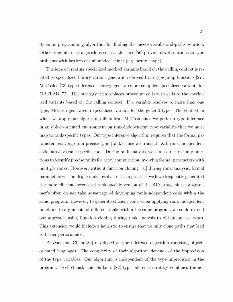
The idea of creating specialized method variants based on the calling context is re-
lated to specialized library variant generation derived from type jump functions [27].
McCosh’s [73] type inference strategy generates pre-compiled specialized variants for
MATLAB [72]. This strategy then replaces procedure calls with calls to the special-
ized variants based on the calling context. If a variable resolves to more than one
type, McCosh generates a specialized variant for the general type. The context in
which we apply our algorithm differs from McCosh since we perform type inference
in an object-oriented environment on rank-independent type variables that we must
map to rank-specific types. Our type inference algorithm requires that the formal pa-
rameters converge to a precise type (rank) since we translate X10 rank-independent
code into Java rank-specific code. During rank analysis, we can use return jump func-
tions to identify precise ranks for array computation involving formal parameters with
multiple ranks. However, without function cloning [31] during rank analysis, formal
parameters with multiple ranks resolve to⊥. In practice, we have frequently generated
the more efficient lower-level rank-specific version of the X10 arrays since program-
mer’s often do not take advantage of developing rank-independent code within the
same program. However, to generate efficient code when applying rank-independent
functions to arguments of different ranks within the same program, we could extend
our approach using function cloning during rank analysis to obtain precise types.
This extension would include a heuristic to ensure that we only clone paths that lead
to better performance.
Plevyak and Chien [84] developed a type inference algorithm targeting object-
oriented languages. The complexity of their algorithm depends of the imprecision
of the type variables. Our algorithm is independent of the type imprecision in the
program. Pechtchanski and Sarkar’s [82] type inference strategy combines the ad-

22
vantages of both static analysis and dynamic optimization. As a result, they can
use a more optimistic approach compared to whole-program static analysis. They
invalidate and reanalyze methods when their optimistic assumptions are false. Their
approach could be advantageous for programs that pass arrays of different ranks to
a method’s formal parameter.
There are differences between this work and past work on APL analysis and opti-
mization [28, 42]. APL, a dynamic language, requires a runtime system with support
for untyped variables (and incurs the overhead of such a system). In contrast, X10
is statically typed, except that an array’s rank/region is treated as part of its value
rather than its type. Further, a major thrust of past work on APL optimization has
been to identify scalar variables. The X10 type system differentiates between scalars
and arrays. Hence, performance improvements for X10 must come from sources other
than scalar identification.

23
Chapter 4
Efficient High-Level X10 Array Computations
The DARPA High Productivity Computing Systems (HPCS) program has challenged
supercomputer vendors to increase development productivity in high-performance sci-
entific computing by a factor of 10 by the year 2010 (the start of the HPCS program
was in 2002). Participants in the HPCS program recognized that introducing new
programming languages is important for meeting this productivity goal, and three
languages have emerged as a result of this initiative: Chapel (Cray), X10 (IBM),
and Fortress (Sun). These languages have significantly improved the programma-
bility of high-performance scientific codes through the use of higher-level language
constructs, object-oriented design, and higher-level abstractions for arrays, loops and
distributions [41]. Chapter 6 demonstrates the programmability benefits of perform-
ing high-level loop iteration in Chapel. Unfortunately, high programmability often
comes at a price of lower performance. The initial implementations of these higher-
level abstractions in the HPCS languages can sometimes result in up to two orders
of magnitude longer execution times when compared to current languages such as C,
Fortran, and Java.
This chapter outlines the novel solutions necessary to generate efficient array com-
putations for high productivity languages, particularly X10. Figure 4.1 shows the X10
compiler structure assumed in our research in the Habanero project [50]. The chap-
ter focuses on compiler analyses and optimizations that improve the performance of
high level array operations in high productivity languages — compilers for other high
productivity languages have a similar structure to Figure 4.1.
In this chapter, we focus on the X10 language abstractions pertinent to high level

24
Bytecode Generator w/ Annotations
Table-driven Scanner & Parser
Parallel Intermed.
Represent. (PIR)
PIR Analyses &
Optimizations
Abstract Syntax Tree (AST)
Point Inlining Array Transformation
Bounds Check Elimination
Rank Analysis Safety Analysis
Bounds Analysis IPA Framework. . .
. . .
Analyses
Opts.
Figure 4.1 : X10 compiler structure
array accesses. There are two aspects of high level array accesses in X10 that are im-
portant for productivity but that also pose significant performance challenges. First,
the high level accesses are performed through Point objects 1 rather than integer in-
dices. Points support an object-oriented approach to specifying sequential and parallel
iterations over general array regions and distributions in X10. As a result, the Point
object encourages programmers to implement reusable high-level iteration abstrac-
tions to productively develop array computations for scientific applications without
having to manage many of the details typical for low-level scientific programming.
However, the creation and use of new Point objects in each iteration of a loop can
be a significant source of overhead. Second, variables containing references to Points
and arrays are rank-independent i.e., by default, the declaration of an array reference
variable in X10 does not specify the rank (or dimension sizes) of its underlying array.
This makes it possible to write rank-independent code in X10, but poses a challenge
for the compiler to generate efficient rank-specific code.
Our solution to the first challenge is to extend the X10 compiler so as to per-
form automatic inlining and scalar replacement of Point objects. We have a hybrid
solution to the second challenge that uses automatic compiler support to infer exact
1Points are described later in Section 4.1

25
ranks of rank-free variables in many X10 programs and programmer support via X10’s
dependent type system to enable the programmer to annotate selected array variable
declarations with additional information for the rank and region of the variable. Sub-
sequently, using dependent type information, the compiler automatically generates
efficient code.
The novel contributions to generating efficient X10 array computations are the
following:
• Object Inlining for Points and Value Types. We utilize the value type property
of points to effectively perform object inlining on all rank-independent points
anywhere in the code. Recall, the value type property prevents objects from
being modified once initially defined. Past work [16, 19, 36, 37, 99, 103] was more
conservative due to potential aliasing of mutable objects or more restrictive by
only allowing inlining of a specific class or enabling object inlining in certain
code regions.
• Runtime Performance. Our compiler optimizations improve X10 applications
with general X10 arrays by 2 orders of magnitude, relative to the open source
reference implementation of X10 [101]. In addition, we demonstrate that our
compiler techniques enable better scalability when scaling from 1 CPU to 64
CPUs.
• Safety Analysis and Array Transformation. The X10 general array supports a
rich set of operations that are not supported by Java arrays. As a result, before
we can convert X10 arrays into Java arrays to boost runtime performance, we
must perform safety analysis. Safety analysis ensures that, for each operation
on an optimized X10 array, there is a semantically equivalent operation for the
Java array.
26
4.1 X10 Language Overview
In this section, we summarize past work on X10 features related to arrays, points,
regions and loops [25], and discuss how they contribute to improved productivity
in high performance computing. Since the introduction of arrays in the fortran
language, the prevailing model for arrays in high performance computing has been as
a contiguous sequence of elements that are addressable via a Cartesian index space.
Further, the actual layout of the array elements in memory is typically dictated by the
underlying language e.g., column major for fortran and row major for C. Though
this low-level array abstraction has served us well for several decades, it also limits
productivity due to the following reasons:
1. Iteration. It is the programmer’s responsibility to write loops that iterate over
the correct index space for the array. Productivity losses can occur when the
programmer inadvertently misses some array elements in the iteration or in-
troduces accesses to non-existent array elements (when array indices are out of
bounds).
2. Sparse Array accesses. Iteration is further complicated when the programmer
is working with a logical model of sparse arrays, while the low level abstraction
supported in the language is that of dense arrays. Productivity losses can occur
when the programmer introduces errors in managing the mapping from sparse
to dense indices.
3. Language Portability. The fact that the array storage layout depends on the
underlying language (e.g., C vs. fortran) introduces losses in productivity
when translating algorithms and code from one language to another.
4. Limitations on Compiler Optimizations. Finally, while the low-level array ab-
straction can provide programmers with more control over performance using
constructs like COMMON blocks and pointer aliasing, there is a productivity

27
loss incurred due to the interference between the low-level abstraction and the
compiler’s ability to perform data transformations for improved performance
(such as array dimension padding and automatic selection of hierarchical stor-
age layouts).
The X10 language addresses these productivity limitations by providing higher-
level abstractions for arrays and loops that build on the concepts of points and regions
(which were in turn inspired by similar constructs in languages such as ZPL [90]). A
point is an element of an n-dimensional Cartesian space (n ≥ 1) with integer-valued
coordinates, where n is the rank of the point. A region is a set of points, and can be
used to specify an array allocation or an iteration construct such as the point-wise
for loop. The benefits of using points inside of for loops include: potential reuse of
common iteration patterns via storage inside of regions and simple point references
replacing multiple loop index variables to access array elements. We use the term,
compact region, to refer to a region for which the set of points can be specified in
bounded space2, independent of the number of points in the region. Rectangular,
triangular, and banded diagonal regions are all examples of compact regions. In
contrast, sparse array formats such as compressed row/column storage are examples
of non-compact regions.
Points and regions are first-class value types [8] — a programmer can declare
variables and create expressions of these types using the operations listed in Figure 4.2
— in X10 [80, 100]. In addition, X10 supports a special syntax for point construction
— the expression, “[a,b,c]”, is implicit syntax for a call to a three-dimensional
point constructor, “point.factory(a,b,c)” — and also for variable declarations.
The declaration, “point p[i,j]” is exploded syntax for declaring a two-dimensional
point variable p along with integer variables i and j which correspond to the first and
second elements of p. Further, by requiring that points and regions be value types,
2For this purpose, we assume that the rank of a region can be assumed to be bounded.

28
Region operations:
R.rank ::= # dimensions in region;
R.size() ::= # points in region
R.contains(P) ::= predicate if region R contains point P
R.contains(S) ::= predicate if region R contains region S
R.equal(S) ::= true if region R and S contain same set of points
R.rank(i) ::= projection of region R on dimension i (a one-dimensional region)
R.rank(i).low() ::= lower bound of i-th dimension of region R
R.rank(i).high() ::= upper bound of i-th dimension of region R
R.ordinal(P) ::= ordinal value of point P in region R
R.coord(N) ::= point in region R with ordinal value = N
R1 && R2 ::= region intersection (will be rectangular if R1,R2 are rectangular)
R1 || R2 ::= union of regions R1 and R2 (may or may not be rectangular,compact)
R1 - R2 ::= region difference (may or may not be rectangular,compact)
Array operations:
A.rank ::= # dimensions in array
A.region ::= index region (domain) of array
A.distribution ::= distribution of array A
A[P] ::= element at point P, where P belongs to A.region
A | R ::= restriction of array onto region R (returns copy of subarray)
A.sum(), A.max() ::= sum/max of elements in array
A1 <op> A2 ::= returns result of applying a point-wise op on array elements,
when A1.region = A2. region
(<op> can include +, -, *, and / )
A1 || A2 ::= disjoint union of arrays A1 and A2
(A1.region and A2.region must be disjoint)
A1.overlay(A2) ::= array with region, A1.region || A2.region,
with element value A2[P] for all points P in A2.region
and A1[P] otherwise.
Figure 4.2 : Region operations in X10

29
the X10 language ensures that individual elements of a point or a region cannot be
modified after construction.
A summary of array operations in X10 can be found in Figure 4.2. A new array
can be created by restricting an existing array to a sub-distribution, by combining
multiple arrays, and by performing point-wise operations on arrays with the same
region. Note that the X10 array allocation expression, “new double[R]”, directly
allocates a multi-dimensional array specified by region R. In its full generality, an array
allocation expression in X10 takes a distribution instead of region. However, we will
ignore distributions in this chapter and limit our attention to single-place executions
although it is straightforward to extend the algorithm to handle distributed arrays.
As an example, consider the Java and code fragments shown in Figure 4.3 for
the Java Grande Forum [54] SOR benchmark3. Note that the i and j loops in the
Java version involve a lot of manipulation of explicit array indices and loops bounds
that can be error prone. In contrast, the rank-specific X10 version uses a single
for loop to iterate over all the points in the inner region (R inner), and also uses
point expressions of the form “t+[-1,0]” to access individual array elements. One
drawback of the point-wise for loop in the X10 version is that (by default) it leads
to an allocation of a new point object in every iteration for the index and for each
subscript expression, thereby significantly degrading performance. Fortunately, the
optimization techniques presented in this chapter enable the use of point-wise loops as
in the bottom of Figure 4.3, while still delivering the same performance as manually
indexed loops as in the top of Figure 4.3.
Figure 4.3 also contains a rank-independent X10 version. In this case, an additional
loop is introduced to compute the weighted sum using all elements in the stencil. Note
that the computation performed by the nested t and s for loops in this version can
be reused for different values of R inner and stencil with different ranks. Although
3For convenience, we use the same name, G, for the allocated array as well as the array used
inside the SOR computation, even though the actual benchmark uses distinct names for both.

30
Java version:
1 double G[][] = new double[M][N];...
2 int Mm1 = M-1; int Nm1 = N-1;
3 for ( int p=0; p<num_iterations; p++) {
4 for ( int i=1; i<Mm1; i++) {
5 double[]Gi=G[i];double[]Gim1=G[i-1];double[]Gip1=G[i+1];
6 for ( int j=1; j<Nm1; j++)
7 Gi[j] = omega_o_four *(Gim1[j]+Gip1[j]+Gi[j-1]+Gi[j+1])
8 + one_minus_omega * Gi[j];
9 }}
X10 version (rank-specific):
1 region R = [0:M-1,0:N-1]; double[.] G = new double[R];...
2 region R_inner = [1:M-2,1:N-2]; // Subregion of R
3 for ( int p=0; p<num_iterations; p++) {
4 for (point t : R_inner) {
5 G[t] = omega_o_four * (G[t+[-1,0]] + G[t+[1 ,0]]
6 + G[t+[0,-1]] + G[t+[0 ,1]]) + one_minus_omega * G[t];
7 }}
X10 version (rank-independent):
1 region R_inner = ... ; // Inner region as before
2 region stencil = ... ; // Set of points in stencil
3 double omega_factor = ...;// Weight used for stencil points
4 for ( int p=0; p<num_iterations; p++) {
5 for (point t : R_inner) {
6 double sum = one_minus_omega * G[t];
7 for (point s : stencil) sum += omega_factor * G[t+s];
8 G[t] = sum;
9 }}
Figure 4.3 : Java Grande SOR benchmark
31
stencil reuse improves productivity, it introduces performance overheads. However,
compiler optimizations [55] can reduce this overhead.
4.2 Improving the Performance of X10 Language Abstrac-
tions
This section has two areas of focus. First, we discuss a compiler optimization we
employ to reduce the overhead of using points in X10. Second, we describe our rank
analysis which can be augmented with X10’s dependent type system to further improve
code generation. As an example, Figure 4.4 contains a simple code fragment illus-
trating how X10 arrays may be indexed with points in lieu of loop indices. Figure 4.5
shows the unoptimized Java output generated by the reference X10 compiler [101]
from the input source code in Figure 4.4. The get and set operations inside the for
loop are expensive, and this is further exacerbated by the fact that they occur within
an innermost loop.
To address this issue, we have a developed an optimization that is a form of object
inlining, specifically tailored for value-type objects. Object inlining [16, 19, 36, 37]
is a compiler optimization for object-oriented languages that transforms objects into
primitive data, and the code that operates on objects into code that operates on
inlined data. Budimlic [16] and Dolby [36] introduced object inlining as an optimiza-
tion for Java and C++. General object inlining requires complex escape analysis
and concrete object and rank-specific array type inference, and the transformation is
irreversible (once unboxed, objects in general cannot be “reboxed”).
However, because points in X10 are value types, we can safely optimize all array
accesses utilizing point objects by replacing them with an object inlined point array
access version. A value object has the property that once the program initializes the
object, it cannot subsequently modify any of the object’s fields. This prevents the
possibility of the code modifying point p in Figure 4.4 in between the assignments – a
situation that would prevent the inlining of the point. As a result, we can inline the

32
1 region arrayRegion1 = [0: datasizes_nz[size ]-1];
2 ...
3 //X10 for loop
4 for (point p : arrayRegion1) {
5 row[p] = rowt[p];
6 col[p] = colt[p];
7 val[p] = valt[p];
8 }
Figure 4.4 : X10 source code of loop example adapted from the Java Grande sparse-matmult benchmark
1 //X10 for loop body translated to Java
2 for ... {
3 ... // Includes code to allocate a new point object for p
4 (row).set((( rowt).get(p)),p);
5 (col).set((( colt).get(p)),p);
6 (val).set((( valt).get(p)),p);
7 }
Figure 4.5 : Source code of loop following translation from unoptimized X10 to Javaby X10 compiler
point object declared in the for loop header. In addition, we can also perform reboxing
on an inlined point when a method invocation expects a point object. Figure 4.6 shows
the results of applying this point optimization to the loop we introduce in Figure 4.4,
and Figure 4.7 shows the resulting Java code.
4.3 Point Inlining Algorithm
We perform a specialized version of object inlining [16] to inline points. There are two
main differences between points and the objects traditionally considered as candidates
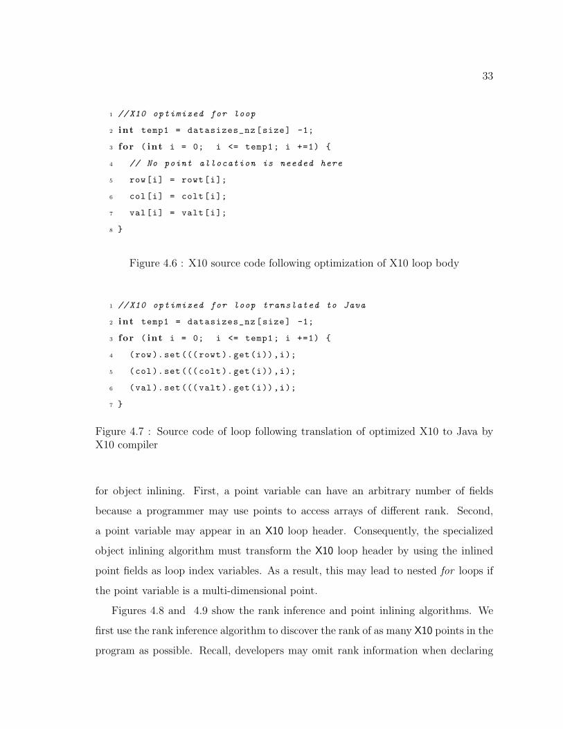
33
1 //X10 optimized for loop
2 int temp1 = datasizes_nz[size] -1;
3 for ( int i = 0; i <= temp1; i +=1) {
4 // No point allocation is needed here
5 row[i] = rowt[i];
6 col[i] = colt[i];
7 val[i] = valt[i];
8 }
Figure 4.6 : X10 source code following optimization of X10 loop body
1 //X10 optimized for loop translated to Java
2 int temp1 = datasizes_nz[size] -1;
3 for ( int i = 0; i <= temp1; i +=1) {
4 (row).set((( rowt).get(i)),i);
5 (col).set((( colt).get(i)),i);
6 (val).set((( valt).get(i)),i);
7 }
Figure 4.7 : Source code of loop following translation of optimized X10 to Java byX10 compiler
for object inlining. First, a point variable can have an arbitrary number of fields
because a programmer may use points to access arrays of different rank. Second,
a point variable may appear in an X10 loop header. Consequently, the specialized
object inlining algorithm must transform the X10 loop header by using the inlined
point fields as loop index variables. As a result, this may lead to nested for loops if
the point variable is a multi-dimensional point.
Figures 4.8 and 4.9 show the rank inference and point inlining algorithms. We
first use the rank inference algorithm to discover the rank of as many X10 points in the
program as possible. Recall, developers may omit rank information when declaring

34
Input: X10 program
Output: rank, a mapping of each X10 array, region and point to its rank
begin
// initialization
worklist = ∅, def = ∅
foreach n ∈ Region, Point, Array dorank(n) = >
worklist = worklist + n
foreach assign a do
if a.rhs ∈ constant thenrank(a.lhs) = a.rhs
def(a.rhs) = def(a.rhs) ∪ a.lhs
foreach call arg c → param f do
if c ∈ constant thenrank(f) = c
def(c) = def(c) ∪ f
// infer ranks
while worklist 6= ∅ doworklist = worklist− n
foreach v ∈ def(n) do
if rank(n) < rank(v) thenrank(v) = rank(n)
worklist = worklist+ v
foreach e in def(v) do worklist = worklist+ e
else if rank(n) 6= rank(v) thenrank(v) = ⊥
worklist = worklist+ v
foreach e in def(v) do worklist = worklist+ e
end
Figure 4.8 : Rank Analysis Algorithm

35
Input: X10 program
Output: inlined points
begin
// flow-insensitive point inlining algorithm
// inlined points
foreach AST node n do if get rank(n) == CONSTANT then
switch typeof(n) do
case pointdeclarationinline(n)
case methodcallargreconstruct point(n)
case pointreferenceinline(n)
case X10loopconvert loop(n)
end
Figure 4.9 : Algorithm for X10 point inlining
X10 points. However, we need to infer rank information to inline the point. We
obtain rank information for points from both point assignments, array accesses, and
array domain information found in X10 loop headers. Then we use safety analysis
to discover which points we can safely inline. Because points have the value type
property, we inline/unbox every safe point with an inferred rank. When encountering
method calls that need a point as an actual parameter, we reconstruct the inlined
point by creating a new point instance, but ensure that this overhead is only incurred
on paths leading to the method calls by allowing the code to work with both original
and unboxed versions of the point. Finally, when possible, we convert a point-wise
X10 loop into a set of nested for loops using the X10 loop’s range information for
each dimension in the region.

36
1 // X10 array declarations with dependent type information
2 // rank ==1 ==> array is one -dimensional
3 // rect ==> array ’s region is dense (rectangular)
4 // zeroBased ==> lower bound of array ’s region is zero
5 double[: rank==1 && rect && zeroBased ] row = ... ;
6 . . .
7 region arrayRegion1 = [0:temp -1];
8 //X10 for loop
9 for (point p : arrayRegion1) {
10 row[p] = rowt[p];
11 col[p] = colt[p];
12 val[p] = valt[p];
13 }
Figure 4.10 : X10 for loop example from Figure 4.4, extended with dependent typedeclarations
4.4 Use of Dependent Type Information for Improved Code
Generation
When examining the Java code generated for the optimization example discussed in
the previous section (Figure 4.7) we see that even though the point object has been
inlined, significant overheads still remain due to the calls to the get/set methods.
These calls are present because by default, the declaration of an array reference vari-
able in X10 does not specify the rank (or dimension sizes) of its underlying array.
This makes it possible to write rank-independent code in X10, but poses a challenge
for the compiler to generate efficient rank-specific code. In this example, all regions
and array accesses are one-dimensional, so it should be possible for the compiler to
generate code with direct array accesses instead of method calls. One solution is to
use the dependent type system [51] of the X10 language specification [79] to enable the
programmer to annotate selected array variable declarations with additional informa-

37
1 //X10 optimized for loop translated to Java
2 for ( int i = 0; i <= temp -1; i +=1) {
3 (( DoubleArray_c)row).arr_[i]=(( DoubleArray_c)rowt).arr_[i];
4 (( DoubleArray_c)col).arr_[i]=(( DoubleArray_c)colt).arr_[i];
5 (( DoubleArray_c)val).arr_[i]=(( DoubleArray_c)valt).arr_[i];
6 }
Figure 4.11 : Source code for loop body translated from X10 to Java by X10 compiler
tion for the rank and region of the variable, and to extend the X10 compiler so as to
generate efficient code in cases where the dependent type information is available. A
key advantage of dependent types over pragmas is that type soundness is guaranteed
statically with dependent types, and dynamic casts can be used to limit the use of
dependent types to performance-critical code regions.
To illustrate this approach, Figure 4.10 contains an extended version of the orig-
inal X10 code fragment in Figure 4.4 with a dependent type declaration shown for
array row. Similar declarations need to be provided for the other arrays as well. The
X10 compiler ensures the soundness of this type declaration i.e., it does not permit
the assignment of any array reference to row that is not guaranteed to satisfy the
properties. We extended the code generation performed by the reference X10 com-
piler [101] to generate the optimized code shown in Figure 4.11 for array references
with the appropriate dependent type declaration. One drawback to relying solely on
the dependent type solution is the performance costs remaining due to our compiler
introducing the casts and indirect field accesses to the backing array arr as shown
in Figure 4.11. Ideally, this dependent type solution should be used to augment a
compiler that deduces rank information automatically (e.g., by propagating rank in-
formation from the array’s allocation site to all its uses). We present our automatic
compiler interprocedural rank inference technique in the next section.

38
4.5 X10 General Array Conversion
The algorithm for converting general X10 arrays into an efficient lower-level imple-
mentation consist of three phases. The first phase, Rank Analysis, infers the concrete
ranks of all the X10 arrays in the program and is described in Section 4.6. The
second phase, Safety Analysis, determines which X10 arrays can be safely converted
into Java arrays, using the rank information computed in Phase 1, and is described
in Section 4.7. Extensions to safety analysis that were designed but not used in our
experimental results are summarized in Section 4.8. The last phase of the algorithm
is the actual conversion of the code manipulating X10 arrays into code operating
directly on the underlying Java arrays (Section 4.9).
4.6 Rank Analysis
This section describes the type inference algorithm that we use to discover the ranks of
X10 arrays. Recall, the generality of X10 arrays enables programmers to develop rank
independent code by omitting array dimensionality at the declaration site. Our whole-
program analysis first uses intraprocedural analysis to capture local rank information
from array assignments. We then perform interprocedural analysis to obtain rank
information arising from both X10 array method arguments and methods returning
X10 arrays. Figure 4.8 shows our rank inference algorithm.
The rank information flows from right to left in the rank inference algorithm.
That is to say, in an assignment, the inferred rank of the left hand side is the lower
(in the type lattice sense) of the rank of the right hand side and the previous rank of
the left hand side. Similarly for a method call (in which the parameter passing can be
conceptually thought of as assignments of actual parameters to formal parameters),
the rank information flows from actual to formal parameters.
The rank inference algorithm can be implemented to run in O(|V | + |E|) time,
where V is the set of array, point, and region variables in the whole program and E is
the set of edges between them. An edge exists between two variables if one defines the

39
other. Theorem 4.6.1 and its proof demonstrate that this algorithm has complexity
O(|V |+ |E|) and preserves program correctness:
Definition A graph is a pair G=(V, E) where:
(1) V is a finite set of nodes.
(2) E are edges and are a subset of V×V.
Definition A lattice is a set L with binary meet operator ∧ such that for all i, j, k
∈ L:
(1) i ∧ i = i (idempotent)
(2) j ∧ i = i ∧ j (commutative)
(3) i ∧ (j ∧ k) = (i ∧ j) ∧ k (associative)
Definition Given a lattice L and i, j ∈ L, i < j iff i ∧ j = i and i 6= j
Definition Given a program P, let T be the set containing point, region and array
types in P and N be the set of variables in P with type t ∈ T such that for all m ∈ N:
(1) DEF(m) is the set of variables in P defined by m.
(2) RANK(m) is the dimensionality associated with m. Each RANK(m) has a
lattice value. There exists a precise rank for m iff RANK(m) 6= > or ⊥.
Theorem 4.6.1. Given a directed graph G where V is the set of program variables of
type array, region, or point, there exists an edge (i,j) between variables i, j ∈ V iff j
∈ DEF(i). The rank analysis algorithm runs in time O(V+E) and preserves program
correctness.
Proof. Initially each node n ∈ V is placed on the worklist with lattice value >. Once
node n is taken off the worklist, n can only be put back on the list iff n ∈ DEF(m)
and m < n or there ∃ a precise rank for both n and m and RANK(n) 6= RANK(m).
In the latter case RANK(n)← ⊥ before we place n back on the worklist. Figure 4.12
shows the rank lattice. Since the lattice is bounded and a node n can only have its

40
┬
┴
N321 ...
Figure 4.12 : Type lattice for ranks
lattice value lowered, each node can only be placed on the worklist a maximum of 3
times. Because we traverse source node edges when lattice value changes, each edge
will be traversed a maximum of 2 times. Therefore, because V is a finite set of nodes,
the algorithm must eventually halt. Since each node n is placed on the worklist a
maximum of 3 times and its edges are traversed a maximum of 2 times, the complexity
is O(V+E). Assuming the whole program is available to the rank analysis algorithm,
the algorithm preserves program correctness. The rank algorithm will produce an
incorrect program iff the algorithm assigns an incorrect precise rank to a program
variable with type array, region, or point. This would only occur when the variable
can have multiple ranks. However, when a variable has multiple ranks, the rank
analysis algorithm assigns the variable ⊥. Therefore, the rank analysis algorithm
produces a correct program.
While rank information, in general, flows from right to left in our rank algorithm,

41
1 //code snippet adapted from JavaGrande X10 Montecarlo
2 // benchmark show benefit of bi -directional
3 //rank inference
4 int nTimeSteps = 1000;
5 region r1 = [0: nTimeSteps -1];
6 double[.] pathVal2;
7 ...
8 this.pathVal2 = new double[r1]; // pathVal2 rank is 1
9 ...
10 // method not called
11 public void set_pathValue(double[.] pv3) {
12 this.pathVal2 = pv3; // assign pv3 pathVal2 ’s rank
13 }
Figure 4.13 : X10 code fragment adapted from JavaGrande X10 montecarlo bench-marks showing when our rank inference algorithm needs to propagate rank informa-tion left to right.
we provide an extension allowing rank information to flow from left to right. This
bi-directional propagation is useful in this context because the extended X10 compiler
performs code generation by translating X10 code into Java. As a result, our X10
array rank analysis extension propagates left hand side assignment rank information
to the right since we are performing code generation by translating rank-independent
code to rank-specific code; thereby requiring the rank on left and right side of the
assignment to be equal. Assuming a compiler performs dead code elimination, our
extended analysis will not discover the precise ranks for more arrays than right to left
rank propagation. Figure 4.13 shows an example of rank information flowing from
left to right.

42
4.7 Safety Analysis
In addition to gathering precise rank information, our type inference algorithm also
employs a safety analysis algorithm to ensure that it is safe to transform an X10
general array into a more efficient representation. The alternate representation used
in this dissertation is the Java array. An X10 array is marked as unsafe if an operation
is performed on it that cannot be supported by Java array operations.
Figure 4.15 shows the high-level description of the safety analysis algorithm we
perform before transforming X10 arrays to Java arrays. The safety analysis algorithm
can be implemented to run in O(|V | + |E|) time, where V is the set of array, point,
and region variables in the whole program and E is the set of edges between them.
An edge exists between two variables if one defines the other. Theorem 4.7.1 and
its proof illustrate that this algorithm has complexity O(|V | + |E|) and preserves
program correctness:
Definition SAFE(i) is > iff i ∈ V and we can either:
(1) convert i into a Java array if i is an X10 array
(2) convert i into a set of size variables to potentially initialize a Java array if i is
a region
otherwise, it is ⊥.
Theorem 4.7.1. Given a directed graph G where V is the set of program variables of
type array or region, there exists an edge between i, j ∈ V where i is the source and j
is the sink iff j ∈ DEF(i). The safety analysis algorithm runs in time O(V+E) and
preserves program correctness.
Proof. Initially each node n ∈ V is placed on the worklist with SAFE(n) = >. Once
node n is taken off the worklist, n can only be put back on the list iff n ∈ DEF(m)
and SAFE(m) < SAFE(n). Since the lattice is bounded (i.e. can only be > or
⊥) and a node n ∈ V can only have its lattice value lowered, each node can only
placed on the worklist a maximum of 2 times. Therefore, because V is a finite set

43
of nodes, the algorithm must eventually halt. The complexity is O(V+E) since we
place only the sink nodes of a source node whose lattice value is lowered on the
worklist. Assuming the whole program is available to the safety analysis algorithm,
the algorithm preserves program correctness. The safety algorithm will produce an
incorrect program iff the algorithm assigns a final lattice value of (safe)> to an unsafe
program variable. This would only occur when the lattice value of a variable was not
updated. However, since all edges are updated when the lattice value changes, all
variables will have the correct lattice value. Therefore, the safety analysis algorithm
produces a correct program.
One detail worth mentioning is that our algorithm performs a bi-directional safety
inference. We utilize safety information on the left hand side of an assignment to
infer safety information for the right hand side and vice versa, thereby reducing
safety analysis to an equivalence partitioning problem. Figure 4.14 highlights the
importance of the bi-directional safety inference. Our algorithm incorporates this
bi-directional strategy for method arguments and formal parameters as well.
4.8 Extensions for Increased Precision
The Rank and Safety analysis algorithms as presented in this section are fairly easy
to understand and implement as linear-time flow-insensitive and context-insensitive
algorithms. We have also designed more complex flow-sensitive and context-sensitive
versions of these algorithms summarized in this section that can potentially compute
more precise rank and safety information, leading to better optimization.
For the set of applications we used as benchmarks in this paper these extensions
do not produce more precise results, thus we chose to omit a more detailed discussion
of these extensions and only include a brief summary here.
Use of SSA Form: The Rank Analysis and Safety Analysis algorithms described
on Figures 4.8 and 4.15 are flow insensitive. Thus, if an array variable a is reassigned
an array of a different rank than before, it will get ⊥ as its rank, which can further

44
1 //code snippet adapted from JavaGrande X10 Montecarlo
2 // benchmark to show benefit of bi -directional
3 // safety inference
4 int this.nTimeSteps = 1000;
5 region r1 = [1: nTimeSteps -1]; //non -zero based
6 region r2 = [0: nTimeSteps -2];
7 double[.] pathVal1;
8 double[.] pathVal2;
9 ...
10 this.pathVal1 = new double[r1]; //r1 is not safe
11 this.pathVal2 = new double[r2]; //r2 is safe
12 ...
13 // propagate safety info left to right in
14 // set_pathValue to ensure pathVal2 is marked unsafe
15 set_pathValue(pathVal2 );
16 ...
17 public void set_pathValue(double[.] pv3) {
18 this.pathVal1 = pv3; //pv3 not safe
19 }
Figure 4.14 : X10 code fragment adapted from JavaGrande X10 montecarlo bench-marks showing when our safety inference algorithm needs to propagate rank informa-tion left to right.
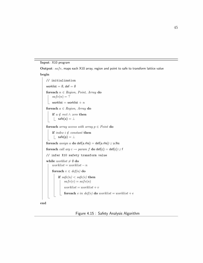
45
Input: X10 program
Output: safe, maps each X10 array, region and point to safe to transform lattice value
begin
// initialization
worklist = ∅, def = ∅
foreach n ∈ Region, Point, Array dosafe(n) = >
worklist = worklist + n
foreach a ∈ Region, Array do
if a /∈ rect ∧ zero thensafe(a) = ⊥
foreach array access with array p ∈ Point do
if index i /∈ constant thensafe(p) = ⊥
foreach assign a do def(a.rhs) = def(a.rhs) ∪ a.lhs
foreach call arg c → param f do def(c) = def(c) ∪ f
// infer X10 safety transform value
while worklist 6= ∅ doworklist = worklist− n
foreach v ∈ def(n) do
if safe(n) < safe(v) thensafe(v) = safe(n)
worklist = worklist+ v
foreach e in def(v) do worklist = worklist+ e
end
Figure 4.15 : Safety Analysis Algorithm

46
get propagated to other variables involved in computation with a. Similarly, if a
variable is marked unsafe for conversion into a Java array, it will prevent conversion
of all occurrences of that variable into a Java array, even if they could potentially
be safely converted in different regions of the code. This source of imprecision can
be eliminated by converting the code into SSA form [14]. The φ nodes in the SSA
form are treated similarly to an assignment: the rank of the variable on the left
hand side gets assigned a merge() of the ranks of all the argument variables to the
φ function. Since rank analysis does not involve any code reorganization, conversion
from the SSA form back into the original form is simple and doesn’t involve any copy
coalescing [17].
Type Jump Functions: The two algorithms, as described here, can propagate
rank and safety information through infeasible paths in the call graph. If a method is
called at one site with an argument of rank 2, and at another site with an argument
of rank 1, the formal array parameter will receive ⊥ as its rank, and it may then
propagate this lower type through the return variable back into the caller code.
This imprecision can be avoided by using type jump functions [27] for method
calls. The idea behind type jump functions is to encapsulate the relation between
the types of actual arguments to a method and the type of the return argument.
Since rank and safety information are essentially types, this method generalization
can be used to increase the precision of the rank and safety analysis algorithms. If a
type jump function describes a method m as accepting the argument of rank R and
returning a value of rank R− 1, then this method can be analyzed independently at
different call sites and will propagate the correct values for the rank, even if the ranks
of the arguments at different call sites are different.
During the conversion of X10 arrays into Java arrays, a method with polymorphic
rank arguments has to be cloned to variants with the specific ranks that are deter-
mined by the call site. The most aggressive approach is to convert as many X10 arrays
as possible by generating as many variants of the method as there are call sites with

47
different sets of ranks for actual arguments. Alternatively, to avoid code explosion,
the compiler can generate a limited set of variants for the most profitable call paths,
and leave the default variant that uses unconverted X10 arrays for the general case.
Type jump functions for the safety analysis, while similar to those for rank anal-
ysis, are simpler since the only two “types” a variable can have are safe and unsafe.
4.9 Array Transformation
Once we have completed the array rank and safety analysis, we begin the transforma-
tion from X10 arrays to the more efficient representation (Java array). There are two
main steps in this process. First, we convert each declared X10 array to our analyzed
precise type. Second, we must convert each such X10ArrayAccess AST node into a
Java ArrayAccess AST node 4. The X10 compiler makes the distinction between these
two types of nodes so that only the X10ArrayAccess can accept a point expression
as an argument. As a result, during the conversion process, we must also convert
any point valued subscript expression into equivalent integer-valued expressions since
we cannot perform a Java array access with a point object. We use a variant of the
Object Inlining [16] optimization (Section 4.3) to convert the X10 points into integer
values [58].
4.10 Object Inlining in Fortress
In Fortress [3], we extend our X10 point inlining algorithm to inline objects of any
type. We aggressively inline all variables whose declared object type has not been
omitted by the programmer since all object types in Fortress represent leaves in
the Fortress type hierarchy (i.e. an object cannot be extended). There are a cou-
ple of differences worth highlighting between the point inlining algorithm and the
extended Fortress object inlining algorithm. In X10, our point inlining algorithm
4AST node refers to the Polyglot Abstract Syntax Tree used in the X10 compiler
48
performs object reconstruction of all inline point method arguments. This solution
is effective since points have the value type property (i.e. once defined, points can-
not subsequently be modified). In Fortress, instead of reconstructing inlined method
arguments, our algorithm synthesizes new methods with inlined formal parameters.
In addition, we extend the X10 point inlining algorithm in Fortress to inline arrays
of objects by replacing the object array with a set of inlined arrays. Future object
inlining work in Fortress includes adding type analysis to identify types for variables
with omitted object types to enable optimizations such as object inlining to be more
effective.

49
Chapter 5
Eliminating Array Bounds Checks with X10
Regions
Many high-level languages perform automatic array bounds checking to improve both
safety and correctness of the code, by eliminating the possibility of an incorrect (or
malicious) code randomly “poking” into memory through an out of bounds array
access or buffer overflow. While these checks are beneficial for safety and correctness,
performing them at run time can significantly degrade performance especially in array-
intensive codes. Two main ways that bounds checks can affect performance are:
1. The Cost of Checks. The runtime may need to check the array bounds when
program execution encounters an array access.
2. Constraining Optimizations. The compiler may be forced to constrain or disable
code optimizations in code region containing checks, in the presence of precise
exception semantics.
Significant effort has been made by the compiler research community to statically
eliminate array bounds checks in higher-level languages when the compiler can prove
that these checks are unnecessary [13, 77, 94]. In this thesis, we take advantage of
the region language construct in X10 to help determine statically when array bounds
checks are not needed in accesses to high-level arrays. In such cases, we annotate the
array access with a noBoundsCheck annotation to signal to a modified version of the
IBM J9 Java Virtual Machine [67] 1 that it can skip the array bounds check for those
1Any JVM can be extended to recognize the noBoundsCheck annotation, but in this thesis our
experiences are reported for a version of the IBM J9 JVM that was modified with this capability.

50
particular array accesses.
X10 regions are particularly suitable for static analysis since they have the value
type property (once defined, they cannot subsequently be modified). This simpli-
fies the compiler task since the region remains unchanged over (say) an entire loop
iteration space, even if the loop contains unanalyzed procedure calls. For example,
consider the following two loops:
double[.] a = new double[[b.low,b.high]];
loop1: for (n=b.low, n <= b.high, n++) {
foo(b);
a[n] = ...
}
region r = [b.low : b.high];
loop2: for (point p : r) {
foo(r);
a[p] = ...
}
In loop1, in addition to proving that there are no modifications to n inside of the
loop other than those imposed by loop iteration itself, one must also prove that neither
low or high are changed inside the loop body (e.g., as a result of a call to foo()) in a
manner that might introduce an illegal array access. However, in loop2, this additional
analysis is unnecessary since the region bounds are immutable. Figure 5.3 illustrates
how X10 regions help array bounds analysis with a code fragment taken from the Java
Grande Forum sparsematmult benchmark [54]. In the sparsematmult example, the
kernel method performs sparse matrix multiplication. Because our analysis discovers
that row and col have the same region, the compiler can apply a transformation that
adds an annotation around col ’s subscript to signal to the Virtual Machine to skip
the bounds check. Inserting this annotation is possible due to the immutability of
X10 regions. A standard Java compiler cannot perform this optimization because it

51
depends on the knowledge that regions are immutable. In addition, determining that
col and row share the same region would require interprocedural analysis, which may
be challenging for a JIT compiler to perform.
In our approach, we insert the noBoundsCheck annotation around an array sub-
script appearing inside the loop if the compiler can establish one of the following
properties:
1. Array Subscript within Region Bound. If the array subscript is a point that
the programmer is using to iterate through region r1 and r1 is a subset of the
array’s region, then the bounds check is unnecessary.
2. Subscript Equivalence. Given two array accesses, one with array a1 and sub-
script s1 and the second with array a2 and subscript s2 : if subscript s1 has the
same value number as s2, s1 executes before subscript s2 and array a1 ’s region
is a subset of a2 ’s region, then the bounds check for a2[s2] is unnecessary.
In Section 7, we show the effects of applying this transformation to a set of bench-
marks. The novel contributions to eliminating bounds checks are the following:
• Building Array Subset Region Relationships. Programmers often define arrays
in scientific codes over either the same domain or a domain subset. Our array
region analysis enables us to discover when the domain of one array is a subset
of the other. This information is useful in eliminating bounds checks when
indexing two arrays with the same index value. Even if we cannot prove that
the first check is superfluous, we can establish redundancy for the second one.
• Region Algebra. The idea of introducing region algebra is to expose computa-
tions involving variables with inherent region associations; thereby proving that
the result of the computation may also become a region association. A defined
variable reference has a region association if the variable satisfies one of the
following properties:

52
1. The variable has type region or is an X10 general array.
2. The variable has type point and appears in the X10 loop header.
3. Program execution assigns the variable a region bound or an offset of the
region bound (e.g. int i = r1.rank(0).high()+1, where r1 is a region , 0
indicates that the bound will be taken from the first dimension, and the
offset is 1, i in this example has a region association).
Only variables of type point, region, X10 array, and integer can have a region
association. We use interprocedural analysis to propagate these region asso-
ciations, allowing us to catch opportunities to eliminate bounds checks that
the JIT compiler would miss due to both a lack of knowledge about region
immutability semantics and the absence of interprocedural bounds analysis in
today’s JIT compiler technology. We principally use the region inequalities n-k
≥ l and n+k ≤ h where n, k are variables with region associations, k ≥ 0, l
and h are respectively the low and high bounds of a region. We apply these
inequalities to cases when k resolves to either a constant or a region where the
rank is 1. In practice, we often discover cases that enable us to further simplify
the inequality expressions such as when n is a region high bound in the first
inequality and the region lower bound is 0. In this case, all we must prove
is that k represents a sub region of n’s region to establish a resulting region
association.
• Array Element Value Ranges. Discovering an array’s range of values can expose
code optimization opportunities. Barik and Sarkar’s [12] enhanced bit-aware
register allocation strategy uses array value ranges to precisely determine how
many bits a scalar variable requires when it is assigned the value of an array
element. In the absence of sparse data structures [71], sparse matrices in lan-
guages like Fortran, C, and Java are often represented by a set of 1-D arrays that
identify the indices of non-zero values in the matrix. This representation usu-

53
ally inhibits standard array bounds elimination analysis because array accesses
often appear in the code with subscripts that are themselves array accesses.
We employ value range analysis to infer value ranges for arrays. Specifically,
our array value range analysis tracks all assignments to array elements. We
ascertain that when program execution assigns an array’s element a value using
the mod function, a loop induction variable, a constant, or array element value,
we can analyze the assignment and establish the bounds for the array’s element
value range. 2
• Value Numbering to Discover Redundant Array Accesses. We use a dominator-
based value numbering technique [15] to find redundant array accesses. We
annotate each array access in the source code with two value numbers. The
first value number represents a value number for the array access. We derive
a value number for the array access by combining the value numbers of the
array reference and the subscript. The second value number represents the
array’s element value range. By maintaining a history of these array access
value numbers we can discover redundant array accesses.
• Using Multiple Code Views to Enhance Bounds Elimination Analysis. We main-
tain two code views. The first is the source code view which the compiler uses
to perform code generation. The second is the analysis code view which we em-
ploy as an abstraction to derive array access bounds checking information. The
second view is helpful to both prune useless source code information and ease
the burden of assigning region value numbers to variables during the analysis
phase. For example, X10 loops are transformed into straight line code blocks.
2Note: when array a1 is an alias of array a2 (e.g. via an array assignment), we assign both a1
and a2 a value range of ⊥, even if a1 and a2 share the same value range, in order to eliminate the
need for interprocedural alias analysis. In the future, value range alias analysis can be added to
handle this case.

54
We generate a loop header point assignment to the loop header region and place
it as the first statement in the code block. When a programmer assigns an array
element a value using the mod function, we transform the analysis code view
by replacing the original assignment with an assignment to a region constructor
where the low bound is 0 and the high bound is the expression on the right
hand side of the mod function - 1. Figure 5.1 provides an example displaying
both the source view and analysis view of the code. Altering the analysis code
view conveniently enhances our elimination bounds analysis without modifying
the source code and affecting code generation.
• Interprocedural Region Analysis with Return Jump Functions. Using the idea of
return type jump functions taken from McCosh [27], we can uncover cases when
a method returns a region that the program passes as a method argument. We
transform the analysis code view by replacing the method call with the region
argument. As a result, even though the method call’s formal parameter region
can be ⊥, the variable on the left hand side of the assignment may resolve to a
more precise region.
• Demonstrating Array View Productivity Benefits. We illustrate the develop-
ment productivity benefit of using array views with a hexahedral cell code ex-
ample [47, 60]. Array views 3 give the programmer the opportunity to work with
multiple views of an array. In practice, programmer’s commonly utilize multiple
array views when they want to manipulate a single array row. We show the
productivity benefit of using array views to switch between a multi-dimensional
and linearized view of the same array.
• Interprocedural Linearized Array Subscript Bounds Analysis. In general, pro-
grammers create linearized arrays to avoid the performance costs incurred when
3As discussed later, array views are different from source and analysis code views.

55
using a multi-dimensional array representation. However, the linearized sub-
scripts can be an impediment to bounds check elimination. To mitigate this
issue, we have the compiler automatically reconstruct multi-dimensional arrays
from the linearized array versions. This ”delinearization” transformation can
enable array bounds analysis using the multi-dimensional array regions. De-
linearization has also been proposed in past work on dependence analysis [70].
However, due to the difficulty in automatically converting some linearized ar-
rays to their multi-dimensional representation, we must perform array bounds
analysis on linearized array subscripts to glean domain iteration information
which we subsequently employ to reduce the number of bounds checks. We
extend this analysis interprocedurally by summarizing local bounds analysis
information for each array.
• Improving Runtime Performance. Using our static array bounds analysis and
automatic compiler annotation insertion to signal the VM when to eliminate
a bounds check, we have improved sequential runtime performance by up to
22.3% over JIT compilation.
5.1 Intraprocedural Region Analysis
Our static bounds analysis first runs a local pass over each method after we translate
the code into a static single assignment form (SSA) [14]. Using a dominator based
value numbering technique [15], we assign value numbers to each point, region, array,
and array access inside the method body. These value numbers represent region
association. Upon completion of local bounds analysis, we map region value numbers
back to the source using the source code position as the unique id. Figure 5.6 shows
the algorithm for the intraprocedural region analysis.
To perform the analysis and transformation techniques described above, we use the
Matlab D framework developed at Rice University [27, 44]. We generate an XML file

56
Source view:
1 region r = [0:99];
2 double[.] a = new double[r];
3 double[.] b = bar(r);
4 for (point p1 : r)
5 b[p1] = foo(new Random ()) % 100;
6 for (point p2 : r)
7 a[p2] = b[p2];
8 // generates random number
9 int foo(Random rand) {
10 return rand.nextInt ();
11 }
12 double[.] bar( region r) {
13 return new double[r];
14 }
Analysis view:
1 r = [0:99];
2 a = r;
3 b = r; // replaced call with returned region argument r
4 p1= r; //next array access: subscript ,array share value number
5 b[p1] = [0:99]; // determines value range for b
6 p2 = r; //next array access: subscript ,array share value number
7 a[p2] = b[p2]; // determines value range for a
8 // generates random number
9 int foo(Random rand) {
10 return rand.nextInt ();
11 }
12 region bar( region r) {
13 return r; // returns formal parameter
14 }
Figure 5.1 : Example displaying both the code source view and analysis view. Wedesigned the analysis view to aid region analysis in discovering array region and valuerange relationships by simplifying the source view.

57
Bytecode Generator w/ Annotations
X10 Abstract Syntax Tree (AST)
XML RegionExtraction &AST Region
Mapping
InterproceduralRegion
Analyses & Optimizations
X10 Abstract Syntax Tree (AST)
Bounds Check Elimination
TeleGen AST SSA Conversion
Region Analysis Value Range Analysis
. . .
. . .
Intr
a. A
naly
ses
Opt
s.
Extensible Markup Language (XML)
XML Generator
Interproc. Region Analysis
Interproc. Value Range Analysis
Inte
r. An
alys
es
X10 Compiler Matlab D Compiler
Figure 5.2 : X10 region analysis compiler framework

58
from the AST of the X10 program, then read this AST within the Matlab D compiler,
convert it into SSA, perform the value numbering based algorithms presented in this
chapter to infer the regions associated with arrays, points and regions in the program,
then use the unique source code position to map the analysis information back into
the X10 compiler. Figure 5.2 summarizes the compiler framework we use for region
analysis.
We build both array region and value region relationships during the local analysis
pass. An array will have a value region if and only if we can statically prove that
every value in the array lies within the bounds of a region. For example, in Figure 5.3,
assuming that the assignment of array values for row is the only row update, analysis
will conclude that row ’s value region is reg1. Our static bounds analysis establishes
this value region relationship because the mod function inherently builds the region
[0:reg1.high()]. Figure 5.4 shows this analysis code view update for array element
assignments to row and col.
We use an implicit, infinitely wide type lattice to propagate the values of the
regions through the program. The lattice is shown on Figure 5.5. In the Matlab D
compiler [44], a φ function performs a meet operation (∧) of all its arguments and
assigns the result to the target of the assignment.
5.2 Interprocedural Region Analysis
If a method returns an expression with a value number that is the same as a formal
parameter value number, analysis will give the array assigned the result of the method
call the value number of the corresponding actual argument at the call site.
Static interprocedural analysis commences once intraprocedural analysis com-
pletes. During program analysis, we work over two different views of the code. The
first is the standard source view which affects code generation. The second is the
analysis view. Changes to the analysis view of the code do not impact code genera-
tion. In Figure 5.3, program execution assigns array x the result of invoking method

59
1 //code fragment is used to highlight
2 // interprocedural array element value
3 //range analysis
4 ...
5 region reg1 = [0:dm[size ]-1];
6 region reg2 = [0:dn[size ]-1];
7 region reg3 = [0:dp[size ]-1];
8 double[.] x = randVec(reg2);
9 double[.] y = new double[reg1];
10 int [.] val = new double[reg3]
11 int [.] col = new double[reg3];
12 int [.] row = new double[reg3];
13 Random R;...
14 for (point p1 : reg3) {
15 // array row has index set in reg3 and value range in reg1
16 row[p1] = Math.abs(R. Int ()) % (reg1.high ()+1);
17 col[p1] = Math.abs(R. Int ()) % (reg2.high ()+1);...
18 }
19 kernel(x,y,val ,col ,row ,..);
21 double[.] randVec( region r1){
22 double[.] a = new double[r1];
23 for (point p2: r1)
24 a[p2] = R.double();
25 return a;
26 }
28 kernel(double[.]x,double[.]y, int [.]val , int [.]col , int [.]row ,..){
29 for (point p3 : col)
30 y[row[p3]]+= x[col[p3]]*val[p3];
31 }
Figure 5.3 : Java Grande Sparse Matrix Multiplication kernel (source view).

60
1 //code fragment is used to highlight
2 // interprocedural array element value
3 //range analysis
4 ...
5 reg1 = [0:dm[size ]-1];
6 reg2 = [0:dn[size ]-1];
7 reg3 = [0:dp[size ]-1];
8 x = reg2; // replaced call with region argument reg2
9 y = reg1;
10 col = reg3;
11 row = reg3;
12 Random R;...
13 p1 = reg3; // replaced X10 loop with assignment to p1
14 row[p1] = [0: reg1.high ()]; // followed by loop body
15 col[p1] = [0: reg2.high ()];// created value range from mod
16 kernel(x,y,col ,row ,..);
17 ...
18 region randVec( region r1){
19 a = r1;
20 p2 = r1; // replaced X10 loop with assignment to p2
21 a[p2] = R.double(); // followed by loop body
22 return r1; // returns formal parameter
23 }
24 kernel(double[.]x,double[.]y, int [.]col , int [.] row ,..){
25 p3 = col; // replaced X10 loop with assignment to p3
26 y[row[p3]]+= x[col[p3]]*val[p3]; // followed by loop body
27 }
Figure 5.4 : Java Grande Sparse Matrix Multiplication kernel (analysis view).

61
[0..1]
┬
┴
[0..0] [0..N,0..M,0..P][0..N,0..M][0..N][0..2][1..1] ... ... ... ...
Figure 5.5 : Type lattice for region equivalence
RandomVector. Because our analysis determines that the method will return the re-
gion the program passes as an argument (assuming region has a lower bound of 0), we
will modify the analysis view by replacing the method call with an assignment to the
argument (reg2 in our example). Figure 5.4 shows this update. When encountering
method calls which our interprocedural regions analysis is not currently analyzing,
we assign each formal argument to the actual argument if and only if the actual ar-
gument has a region association. Each actual argument can have one of the following
three region states:
• If the method argument is a X10 array, region, or point, then the argument will
be in the full region state.
• The method argument has a partial region state when it represents the high or
low bound of a linear region.

62
Input: X10 program
Output: region, a local mapping of each X10 array, region and point to its region value number
begin
// initialization
foreach CFG node c do
foreach n ∈ Region, Point, Array doregion(n) = >
// infer X10 region mapping
foreach a ∈ assign do
if a ∈ φ function then
region(a.def)←a.numargs∧
i=0
region(a.arg(i))
else if a.rhs ∈ constant thenregion(a.lhs) = a.rhs
elseregion(a.rhs) = region(a.rhs)
foreach a /∈ assign doregion(a) = a;
end
Figure 5.6 : Intraprocedural region analysis algorithm builds local region relation-ships.

63
• If the method argument does not fall within the first two cases, then we assign ⊥
to the argument (no region association). This distinction minimizes the number
of variables that we need to track during region analysis.
In addition to analyzing the code to detect region equivalence, we augment the
analysis with extensions to support sub-region relationships. Inferring sub-region re-
lationships between arrays, regions and points is similar in structure to region equiv-
alence inference analysis, but is different enough to warrant a separate discussion. As
with the interprocedural region equivalence analysis, there is an implicit type lattice,
but this time the lattice is unbounded in height as well as in width. The lattice is
shown on Figure 5.7.
The lattice is defined as follows: there is an edge between regions A and B in the
lattice if and only if the two regions are of the same dimensionality, and region A is
completely contained within region B. During our analysis, we compute on demand
an approximation of the relation on Figure 5.7; if we cannot prove that a region A is
a sub-region of region B, then A ∧B = ⊥.
In addition, our analysis is flow-insensitive for global variables. When static analy-
sis determines that a global variable might be involved in multiple region assignments
involving different regions, the region for the variable becomes ⊥. In the future, we
can extend the algorithm to assign the variable the region intersection instead of ⊥.
Figure 5.8 presents pseudo code for the static interprocedural region analysis algo-
rithm. The interprocedural region analysis algorithm can be implemented to run in
O(|V |+ |E|) time, where V is the number of array, point, and region variables in the
whole program and E is the number of edges between them. An edge exists between
two variables if one defines the other. Theorem 5.2.1 and its proof shows that this
algorithm has complexity O(|V |+ |E|) and preserves program correctness:
Definition A graph is a pair G=(V, E) where:
(1) V is a finite set of nodes.
(2) E are edges and are a subset of V×V.
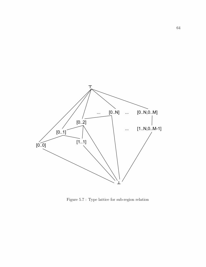
64
[0..1]
┬
┴
[0..0]
[1..N,0..M-1]
[0..N,0..M][0..N]
[0..2]
[1..1]
... ... ...
......
Figure 5.7 : Type lattice for sub-region relation

65
Definition A lattice is a set L with binary meet operator ∧ such that for all i, j, k
∈ L:
(1) i ∧ i = i (idempotent)
(2) j ∧ i = i ∧ j (commutative)
(3) i ∧ (j ∧ k) = (i ∧ j) ∧ k (associative)
Definition Given a lattice L and i, j ∈ L, i < j iff i ∧ j = i and i 6= j
Definition Given a program P, let T be the set containing point, region and array
types in P and N be the set of variables in P with type t ∈ T such that for all m ∈ N:
(1) DEF(m) is the set of variables in P defined by m.
(2) REG(i) is the region associated with i. There ∃ precise region for i iff i ∈ V
and REG(i) 6= > or ⊥
Theorem 5.2.1. Given a directed graph G where V is the set of program variables
of type array or region, there exists an edge E between i, j ∈ V where i is the source
and j is the sink iff j ∈ DEF(i). The region analysis algorithm runs in time O(V+E)
and preserves program correctness.
Proof. Initially each node n ∈ V is placed on the worklist with lattice value >. Once
node n is taken off the worklist, n can only be put back on the list iff n ∈ DEF(m) and
m < n or there ∃ precise regions for bothn and m and REG(n) 6= REG(m). In the
latter case n← ⊥ before we place n back on the worklist. Since the lattice is bounded
and a node n can only have its lattice value lowered, each node can only be placed
on the worklist a maximum of 3 times. Because we traverse source node edges when
lattice value changes, each edge will be traversed a maximum of 2 times. Therefore,
because V is a finite set of nodes, the algorithm must eventually halt. Since each
node n is placed on the worklist a maximum of 3 times and its edges are traversed
a maximum of 2 times, the complexity is O(V+E). Note that i ∧ j = ⊥ even when
i ⊂ j. Assuming the whole program is available to the region analysis algorithm,
66
the algorithm preserves program correctness. The region algorithm will produce an
incorrect program iff the algorithm assigns an incorrect precise region to a program
variable with type array or region. This would only occur when the variable can have
multiple regions. However, when a variable has multiple regions, the region analysis
algorithm assigns the variable ⊥. Therefore, the region analysis algorithm produces
a correct program.
5.3 Region Algebra
Often in scientific codes, loops iterate over the interior points of an array. If through
static analysis we can prove that loops are iterating over sub-regions of an array,
we can identify the bounds checks for those array references as superfluous. We use
the example on Figure 5.9 to highlight the benefits of employing region algebra to
build variable region relationships. Figure 5.10 shows the algorithm for region algebra
analysis.
When our static region analysis encounters the dgefa method call with a region
high bound argument in Figure 5.9, analysis will assign dgefa’s formal parameter n the
high bound of region1 ’s second dimension and a the region region1. We shall hence-
forth refer to the region representing region1 ’s second dimension as region1 2dim.
Inside dgefa’s method body, analysis will categorize nm1 as a region bound and
region3 as a sub-region of region1 2dim when inserting it in the region tree.
Next, we assign array col k the region region1 2dim and categorize kp1 as a sub-
region of region1 2dim. When static region analysis examines the binary expression
n-kp1 on the right hand side of the assignment to var1, it discovers that the n is
region1 2dim.hbound() and kp1 is a sub region of region1 2dim. As a result, we
can use region algebra to prove that this region operation will return a region r
where: r.lbound() ≥ region1 2dim.lbound() and r.bound() ≤ region1 2dim.hbound().
Consequently, var1 will be assigned region1 2dim.

67
Input: X10 program
Output: region, a mapping of each X10 array, region and point to its region
begin
// initialization
worklist = ∅, def = ∅
foreach n ∈ Region, Point, Array doregion(n) = >
worklist = worklist + n
foreach assign a do
if a.rhs ∈ constant thenregion(a.lhs) = a.rhs
def(a.rhs) = def(a.rhs) ∪ a.lhs
foreach call arg c → param f do
if c ∈ constant thenregion(f) = c
def(c) = def(c) ∪ f
// infer X10 region mapping
while worklist 6= ∅ doworklist = worklist− n
foreach v ∈ def(n) do
if region(n) < region(v) thenregion(v) = region(n)
worklist = worklist+ v
foreach e in def(v) do worklist = worklist+ e
else if region(n) 6= region(v) thenregion(v) = ⊥
worklist = worklist+ v
foreach e in def(v) do worklist = worklist+ e
end
Figure 5.8 : Interprocedural region analysis algorithm maps variables of type X10array, point, and region to a concrete region.

68
Finally, analysis determines that var2 ’s region is a sub-region of region1 2dim. As
a result, when analysis encounters the daxpy call it will assign daxpy formal parameter
dx the region region1 2dim and formal parameter dax reg the same region as var2
enabling us to prove and signal to the VM that the bounds check for the array access
dx[p2] in daxpy ’s method body is unnecessary.
5.4 Improving Productivity with Array Views
In the Habanero project [50], we have proposed an extention to X10 arrays called
array views. A programmer can exploit the array’s view to traverse an alternative
representation of the array. Prevalent in scientific codes is the expression of the form a
= b[i] which often assigns the variable a row i of array b when b is a two-dimensional
array. Array views can extend this idea by providing an alternate view for the entire
array. The following code snippet shows an array view example:
double[.] ia = new double[[1:10,1:10]];
double[.] v = ia.view([10,10],[1:1]);
v[1] = 42;
print(ia[10,10]);
The programmer declares array ia to be a 2-dimensional array. Next, the pro-
grammer creates the array view v to represent a view of 1 element in the array ia.
This essentially introduces a pointer to element ia[10,10]. Subsequently, when the
programmer modifies the array v, array ia is also modified resulting in the print
statement yielding the value 42. We will use a hexahedral cells code [47] as a running
example to illustrate the productivity benefits of using array views in practice. Fig-
ure 5.11 shows the initialization of multi-dimensional arrays x, y, and z. Note: Only
1 for loop header would be needed (for point p : reg mesh 3D) if statements appear
in only the innermost loop.

69
1 //code fragment is used to highlight
2 // interprocedural region analysis using region algebra
3 int n = dsizes[size];
4 int ldaa = n;
5 int lda = ldaa + 1;
6 ...
7 region region1 = [0:ldaa -1,0:lda -1];...
8 double[.] a = new double[region1 ]...
9 info = dgefa(a, region1.rank(1). high(), ipvt);
10 //dgefa method , lufact kernel
11 int dgefa(double[.] a, int n, int [.] ipvt ){...
12 nm1 = n - 1;...
13 region region3 = [0:nm1 -1];...
14 for (point p1[k] : region3) {
15 col_k = RowView(a,k);...
16 kp1 = k + 1...
17 int var1 = n-kp1;
18 region var2 = [kp1:n];...
19 daxpy(var1 ,col_k ,kp1 ,var2 ,...);...
20 }
21 }
22 ...
23 //daxpy method
24 void daxpy( int n,double[.]dx , int dx_off , region dax_reg ,..){..
25 for (point p2 : dax_reg)
26 dy[p2]+= da*dx[p2 ];...
27 }
Figure 5.9 : Java Grande LU factorization kernel.

70
Input: X10 program
Output: region, a mapping of each X10 array, region, point and int to its region association
begin
// initialization
worklist = ∅, def = ∅
foreach n ∈ Region, Point, Array, int doregAssoc(n) = >
worklist = worklist + n
foreach assign a do
if a.rhs ∈ constant ∨ bound thenregAssoc(a.lhs) = a.rhs
def(a.rhs) = def(a.rhs) ∪ a.lhs
foreach call arg c → param f do
if c ∈ constant ∨ bound thenregAssoc(f) = a.rhs
def(c) = def(c) ∪ f
// infer X10 region mapping
while worklist 6= ∅ doworklist = worklist− n
foreach v ∈ def(n) do
if regAssoc(n) < regAssoc(v) thenregAssoc(v) = regAssoc(n)
worklist = worklist+ v
foreach e in def(v) do worklist = worklist+ e
else if regAssoc(n) 6= regAssoc(v) thenregAssoc(v) = ⊥
worklist = worklist+ v
foreach e in def(v) do worklist = worklist+ e
end
Figure 5.10 : Region algebra algorithm discovers integers and points that have aregion association.

71
Figure 5.12 illustrates one problem that arises when programmers utilize an array
access as a multi-dimensional array subscript. Since the subscript returns an integer,
the developer cannot use the subscript for multi-dimensional arrays. As a result,
the programmer must rewrite this code fragment by first replacing the 3-dimensional
arrays x, y and z with linearized array representations. Subsequently, the developer
needs to modify the array subscripts inside the innermost loop of Figure 5.11 with the
more complex subscript expression for the linearized arrays. While this solution is
correct, we can implement a more productive solution using X10 array views as shown
in Figure 5.13. This solution enables programmers to develop scientific applications
with multi-dimensional array computations in the presence of subscript expressions
returning non-tuple values.
Figure 5.14 shows the result of applying our array transformation described in Sec-
tion 4.9 to the hexahedral cells code example. The process converts the 3-dimensional
X10 arrays into 3-dimensional Java arrays when analysis determines it is safe to do
so. This compilation pass does not transform the X10 arrays x, y, z, xv, yv, and zv
because of their involvement in the X10 array.view() method call. There is not a
semantically-equivalent Java method counterpart for the X10 array.view() method.
One drawback of array views as presented is that safety analysis marks the view’s tar-
get array as unsafe to transform. The array transformation pass does convert the X10
general arrays p1 and p2 in Figure 5.14 into 3-dimensional Java array representations.
Although 3-dimensional array accesses in Java are inefficient, this transformation still
delivers more than a factor of 3 speedup over the code version with only X10 general
arrays.
We can achieve even better performance by linearizing the 3-dimensional Java
arrays. Figure 5.15 displays the code after Java array linearization. The Lin-
earViewAuto call indicates where the compiler has automatically linearized a multi-
dimensional X10 array whereas the LinearViewHand method invocation indicates
where the programmer has requested a linear view of a multi-dimensional region.
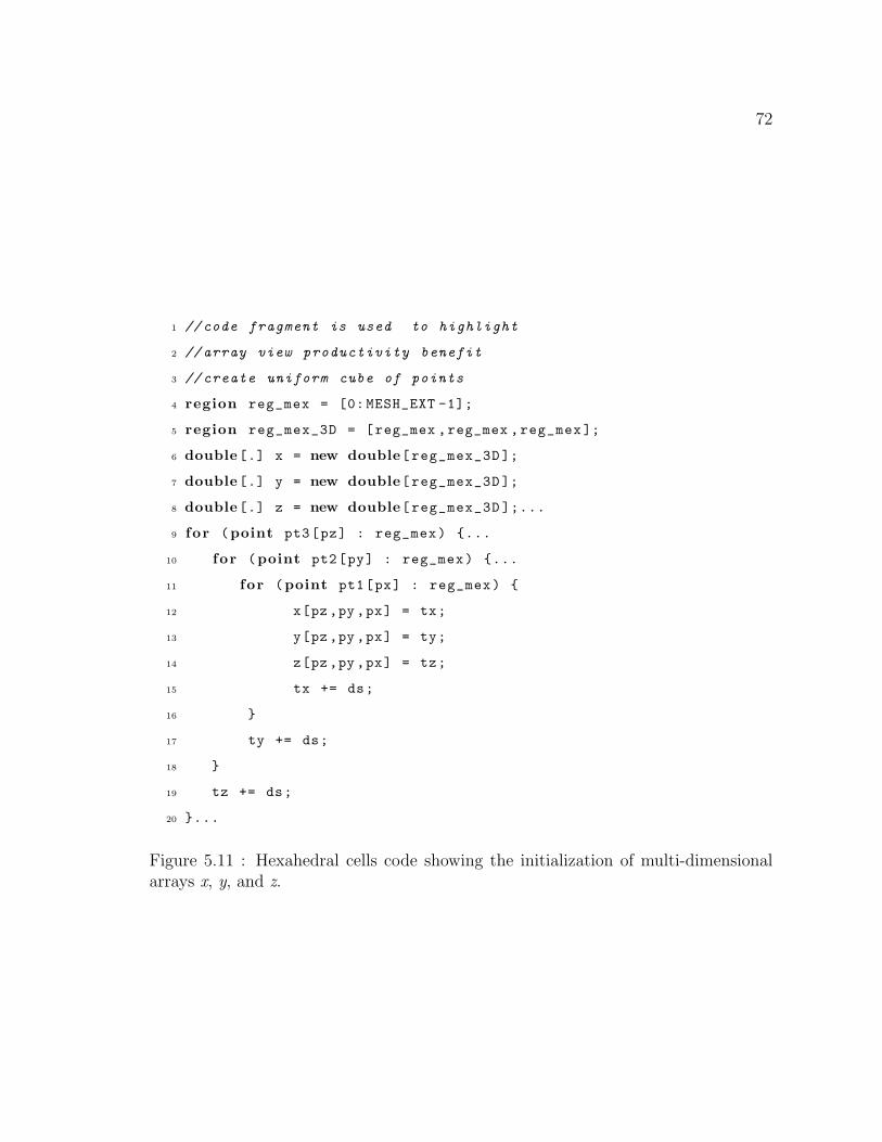
72
1 //code fragment is used to highlight
2 //array view productivity benefit
3 // create uniform cube of points
4 region reg_mex = [0: MESH_EXT -1];
5 region reg_mex_3D = [reg_mex ,reg_mex ,reg_mex ];
6 double[.] x = new double[reg_mex_3D ];
7 double[.] y = new double[reg_mex_3D ];
8 double[.] z = new double[reg_mex_3D ];...
9 for (point pt3[pz] : reg_mex) {...
10 for (point pt2[py] : reg_mex) {...
11 for (point pt1[px] : reg_mex) {
12 x[pz ,py ,px] = tx;
13 y[pz ,py ,px] = ty;
14 z[pz ,py ,px] = tz;
15 tx += ds;
16 }
17 ty += ds;
18 }
19 tz += ds;
20 }...
Figure 5.11 : Hexahedral cells code showing the initialization of multi-dimensionalarrays x, y, and z.

73
1 //code fragment highlights array view productivity benefit
2 region reg_mex = [0: MESH_EXT -1];
3 region reg_mex_linear =[0: MESH_EXT*MESH_EXT*MESH_EXT -1];
4 double[.] x = new double[reg_mex_linear -];
5 double[.] y = new double[reg_mex_linear ];
6 double[.] z = new double[reg_mex_linear ];...
7 for (point pt3[pz] : reg_mex) {...
8 for (point pt2[py] : reg_mex) {...
9 for (point pt1[px] : reg_mex) {
10 //using less productive linearized array access
11 x[px+MESH_EXT *(py + MESH_EXT*pz)] = tx;
12 y[px+MESH_EXT *(py + MESH_EXT*pz)] = ty;
13 z[px+MESH_EXT *(py + MESH_EXT*pz)] = tz;
14 tx += ds;
15 }
16 ty += ds;
17 }
18 tz += ds;
19 }...
20 region reg_br = [0: MESH_EXT -2];
21 region reg_br_3D = [reg_br , reg_br , reg_br ];
22 int [.] p1 ,p2 = new int [reg_br_3D ];...
23 //would be invalid if x, y, and z were 3-D arrays
24 for (point pt7 : reg_br) {
25 ux = x[p2[pt7]] - x[p1[pt7 ]];
26 uy = y[p2[pt7]] - y[p1[pt7 ]];
27 uz = z[p2[pt7]] - z[p1[pt7 ]]; ...
28 }
Figure 5.12 : Hexahedral cells code showing that problems arise when representingarrays x, y, and z as 3-dimensional arrays due to programmers indexing into thesearrays using an array access returning integer value instead of a triplet.

74
1 //code fragment highlights array view productivity benefit
2 region reg_mex = [0: MESH_EXT -1];
3 region reg_mex_3D = [reg_mex ,reg_mex ,reg_mex ];
4 double[.] x,y,z = new double[reg_mex_3D ];...
5 for (point pt3[pz] : reg_mex) {...
6 for (point pt2[py] : reg_mex) {...
7 for (point pt1[px] : reg_mex) {
8 x[pz,py,px] = tx; //use productive multi -D
9 y[pz,py,px] = ty; // access with array views
10 z[pz,py,px] = tz;
11 tx += ds;
12 }
13 ty += ds;
14 }
15 tz += ds;
16 }...
17 region reg_br = [0: MESH_EXT -2];
18 region reg_br_3D = [reg_br , reg_br , reg_br ];
19 int [.] p1 ,p2 = new int [reg_br_3D ];...
20 region reg_linear =[0: MESH_EXT*MESH_EXT*MESH_EXT -1];
21 double[.] xv = x.view ([0 ,0] ,[0: reg_linear ];
22 double[.] yv = y.view ([0 ,0] ,[0: reg_linear ];
23 double[.] zv = z.view ([0 ,0] ,[0: reg_linear ];
24 for (point pt7: reg_br) {
25 ux = xv[p2[pt7]] - xv[p1[pt7 ]];
26 uy = yv[p2[pt7]] - yv[p1[pt7 ]];
27 uz = zv[p2[pt7]] - zv[p1[pt7 ]];...
28 }
Figure 5.13 : Array views xv, yv, and zv enable the programmer to productivityimplement 3-dimensional array computations inside the innermost loop.

75
1 //code fragment highlights X10 to Java array translation
2 region reg_mex = [0: MESH_EXT -1];
3 region reg_mex_3D = [reg_mex ,reg_mex ,reg_mex ];
4 double[.] x,y,z = new double[reg_mex_3D ];...
5 for (point pt3[pz] : reg_mex) {...
6 for (point pt2[py] : reg_mex) {...
7 for (point pt1[px] : reg_mex) {
8 x[pz,py,px] = tx; //use productive multi -D
9 y[pz,py,px] = ty; // access with array views
10 z[pz,py,px] = tz;
11 tx += ds;
12 }
13 ty += ds;
14 }
15 tz += ds;
16 }...
17 region reg_br = [0: MESH_EXT -2];
18 region reg_br_3D = [reg_br , reg_br , reg_br ];
19 int [][][] p1 ,p2 = new int [reg_br_3D ];...
20 region reg_linear =[0: MESH_EXT*MESH_EXT*MESH_EXT -1];
21 double[.] xv = x.view ([0 ,0] ,[0: reg_linear ];
22 double[.] yv = y.view ([0 ,0] ,[0: reg_linear ];
23 double[.] zv = z.view ([0 ,0] ,[0: reg_linear ];
24 for (point pt7[i,j,k]: reg_br) {
25 ux = xv[p2[i][j][k]] - xv[p1[i][j][k]] ;
26 uy = yv[p2[i][j][k]] - yv[p1[i][j][k]] ;
27 uz = zv[p2[i][j][k]] - zv[p1[i][j][k]] ;...
28 }
Figure 5.14 : We highlight the array transformation of X10 arrays into Java arraysto boost runtime performance. In this hexahedral cells volume calculation code frag-ment, our compiler could not transform X10 arrays x, y, z, xv, yv, zv into Java arraysbecause the Java language doesn’t have an equivalent array view operation.
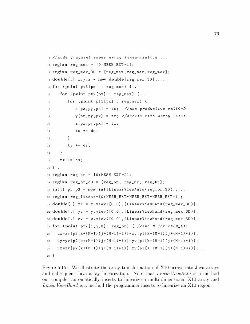
76
1 //code fragment shows array linearization ...
2 region reg_mex = [0: MESH_EXT -1];
3 region reg_mex_3D = [reg_mex ,reg_mex ,reg_mex ];
4 double[.] x,y,z = new double[reg_mex_3D ];...
5 for (point pt3[pz] : reg_mex) {...
6 for (point pt2[py] : reg_mex) {...
7 for (point pt1[px] : reg_mex) {
8 x[pz,py,px] = tx; //use productive multi -D
9 y[pz,py,px] = ty; // access with array views
10 z[pz,py,px] = tz;
11 tx += ds;
12 }
13 ty += ds;
14 }
15 tz += ds;
16 }...
17 region reg_br = [0: MESH_EXT -2];
18 region reg_br_3D = [reg_br , reg_br , reg_br ];
19 int [] p1 ,p2 = new int [LinearViewAuto(reg_br_3D )];...
20 region reg_linear =[0: MESH_EXT*MESH_EXT*MESH_EXT -1];
21 double[.] xv = x.view ([0,0],[ LinearViewHand(reg_mex_3D )];
22 double[.] yv = y.view ([0,0],[ LinearViewHand(reg_mex_3D )];
23 double[.] zv = z.view ([0,0],[ LinearViewHand(reg_mex_3D )];
24 for (point pt7[i,j,k]: reg_br) { //sub M for MESH_EXT
25 ux=xv[p2[k+(M-1)(j+(M-1)*i)]-xv[p1[k+(M-1)(j+(M-1)*i)];
26 uy=yv[p2[k+(M-1)(j+(M-1)*i)]-yv[p1[k+(M-1)(j+(M-1)*i)];
27 uz=zv[p2[k+(M-1)(j+(M-1)*i)]-zv[p1[k+(M-1)(j+(M-1)*i)];..
28 }
Figure 5.15 : We illustrate the array transformation of X10 arrays into Java arraysand subsequent Java array linearization. Note that LinearViewAuto is a methodour compiler automatically inserts to linearize a multi-dimensional X10 array andLinearViewHand is a method the programmer inserts to linearize an X10 region.

77
Automatic linearization on the hexahedral code fragment further decreased the exe-
cution time by 12%. However, there are opportunities to realize faster execution times
by optimizing away the X10 array.view() methods, enabling the array transformation
strategy to convert and linearize the remaining X10 general arrays. We observe that
the array views in this code fragment are themselves X10 linearized representations
of the view target X10 array. If there are no other conditions preventing our com-
piler from performing array conversion and linearization on these X10 general arrays,
linearizing these X10 general array at the declaration site introduces redundant lin-
earization operations, namely these X10 array.view() in Figure 5.15. As a result,
we can optimize away the array views by replacing them with an assignment to the
whole array. Figure 5.16 provides the final source output for the hexahedral cells code
fragment. Performing this optimization enables us to achieve an additional factor of
7 speedup relative to the previous best execution time and an order of magnitude
improvement over the code version with only X10 general arrays.
5.5 Interprocedural Linearized Array Bounds Analysis
Our array bounds analysis algorithm as described in Section 5.1 and Section 5.2 makes
heavy use of X10 points and regions to discover when bounds checks are superfluous.
In general, the programmer iterates through the elements in an array by implementing
an X10 for loop whose header contains both a point declaration p1 and the region r1
containing the set of points defining p1. As a result, when encountering an array access
with subscript p1, if our array bounds analysis can establish a subset relationship
between the array’s region and region r1, our analysis can signal the VM that a
bounds check for this array access is superfluous.
In scientific codes, application developers typically linearize multi-dimensional ar-
ray representations to deliver improved runtime efficiency. One drawback to this
scheme is that to support this approach, programmers must often introduce com-
plex subscript expressions when accessing elements in the linearized array to ensure

78
1 //code fragment shows opt with array linearization
2 region reg_mex = [0: MESH_EXT -1];
3 region reg_mex_3D = [reg_mex ,reg_mex ,reg_mex ];
4 double[.] x,y,z = new double[LinearViewAuto(reg_mex_3D )];...
5 for (point pt3[pz] : reg_mex) {...
6 for (point pt2[py] : reg_mex) {...
7 for (point pt1[px] : reg_mex) {
8 x[pz,py,px] = tx; //use productive multi -D
9 y[pz,py,px] = ty; // access with array views
10 z[pz,py,px] = tz;
11 tx += ds;
12 }
13 ty += ds;
14 }
15 tz += ds;
16 }...
17 region reg_br = [0: MESH_EXT -2];
18 region reg_br_3D = [reg_br , reg_br , reg_br ];
19 int [] p1 ,p2 = new int [LinearViewAuto(reg_br_3D )];...
20 region reg_linear =[0: MESH_EXT*MESH_EXT*MESH_EXT -1];
21 double[] xv = x;
22 double[] yv = y;
23 double[] zv = z;
24 for (point pt7[i,j,k]: reg_br) { //sub M for MESH_EXT
25 ux=xv[p2[k+(M-1)(j+(M-1)*i)]-xv[p1[k+(M-1)(j+(M-1)*i)];
26 uy=yv[p2[k+(M-1)(j+(M-1)*i)]-yv[p1[k+(M-1)(j+(M-1)*i)];
27 uz=zv[p2[k+(M-1)(j+(M-1)*i)]-zv[p1[k+(M-1)(j+(M-1)*i)];..
28 }
Figure 5.16 : We show the final version for the Hexahedral cells code which demon-strates the compiler’s ability to translate X10 arrays into Java arrays in the presenceof array views.

79
correctness. As a result, our array bounds analysis loses the ability to make the
straightforward comparison between an array’s region and its point subscript com-
prising the loop iteration space to discover unnecessary bounds checks for linearized
arrays. Ideally, from our compiler’s perspective, we should convert the linearized
arrays back into the multi-dimensional representation, enabling the bounds analysis
to treat linearized and multi-dimensional array accesses in the same way. However,
automatically converting linearized arrays to a multi-dimensional representation is
certainly not trivial and in some cases may not be possible.
Figure 5.17 illustrates an MG code fragment where the application developer lin-
earizes a 3-dimensional array to boost runtime performance. This example shows
why our current array bounds analysis cannot rely on the compiler automatically
converting linearized arrays to X10 multi-dimensional arrays because the range for
each dimension in this case cannot be established. As a result, our bounds analysis
must be extended if we want to analyze linearized array accesses to discover useless
bound checks. Figure 5.18 highlights another extension to the array bounds analy-
sis we previously described in Section 5.1 and Section 5.2. Studying the MG code
fragment reveals that all the accesses to array r inside method psinv are redundant.
Our array bounds analysis adds the following requirements to prove that r’s bounds
checks are redundant:
• The array region summary for psinv’s formal parameter r is a subset of the
region summary for zero3’s formal parameter z . The region summary for a
given array and procedure defines the valid array index space inside the proce-
dure for which a bounds check is useless. The region summary contains only an
index set that must execute when the programmer invokes this method. We do
not include array accesses occurring inside conditional statements in the region
summary.
• The region representing the actual argument of psinv’s formal parameter r
is a subset of the region representing the actual argument for zero3’s formal

80
1 //MG code fragment is used to highlight
2 // challenge of converting linearized
3 // arrays to a multi -dimensional representation
4 ...
5 // create linearized array
6 int nm = 2+(1<<lm);
7 int nv = (2+(1<< ndim1 ))*(2+(1 < < ndim2 ))*(2+(1 < < ndim3 ));
8 int nr = (8*(nv+nm*nm+5*nm+7*lm ))/7;
9 region reg_nr = [0:nr -1]; //non -trivially 3-D reconstruction
10 double[.] u = new double[reg_nr ];...
11 zero3(u, 0, n1, n2, n3);
12 ...
13 void zero3(double[.] z, int off , int n1 , int n2 , int n3) {
14 for (point p1[i3 ,i2 ,i1]: [0:n3 -1,0:n2 -1,0:n1 -1])
15 z[off+i1+n1*(i2+n2*i3)] = 0.0;
16 }
Figure 5.17 : Array u is a 3-dimensional array that the programmer has linearizedto improve runtime performance. Converting the linearized array into an X10 3-dimensional array would remove the the complex array subscript expression insidethe loop in zero3’s method body and enable bounds analysis to attempt to discovera superfluous bounds check. However, this example shows it may not be possible toalways perform the conversion.
parameter z.
• The program must call zero3 before calling psinv.
• Since our analysis modifies psinv’s actual method body, the previous require-
ments must hold on all calls to psinv.
These requirements enable our interprocedural region analysis to delinearize array
accesses into region summaries and to propagate the region summary information to
discover redundant bounds checks.

81
1 //MG code fragment hightlights opportunity to eliminate
2 //bound checks with procedure array bound summaries
3 int nm = 2+(1<<lm);
4 int nv = (2+(1<< ndim1 ))*(2+(1 < < ndim2 ))*(2+(1 < < ndim3 ));
5 int nr = (8*(nv+nm*nm+5*nm+7*lm ))/7;
6 region reg_nr = [0:nr -1];
7 double[.]u=new double[reg_nr ]; // create linearized array
8 zero3(u, 0, n1, n2, n3);
9 psinv(u, 0, n1, n2, n3);
10 ...
11 void zero3(double[.] z, int off , int n1, int n2 , int n3) {
12 for (point p1[i3 ,i2 ,i1]: [0:n3 -1,0:n2 -1,0:n1 -1])
13 z[off+i1+n1*(i2+n2*i3)] = 0.0;
14 }...
15 void psinv(double[.] r, int off , int n1, int n2 , n3) {...
16 for (point p40[i3 ,i2]: [1:n3 -2,1:n2 -2]) {
17 for (point p41[i1] : [0:n1 -1]) {
18 r1[p41] = r[roff+i1+n1*(i2 -1+n2*i3)]
19 + r[roff+i1+n1*(i2+1+n2*i3)]
20 + r[roff+i1+n1*(i2+n2*(i3 -1))]
21 + r[roff+i1+n1*(i2+n2*(i3 +1))];
22 r2[p41] = r[roff+i1+n1*(i2 -1+n2*(i3 -1))]
23 + r[roff+i1+n1*(i2+1+n2*(i3 -1))]
24 + r[roff+i1+n1*(i2 -1+n2*(i3+1))]
25 + r[roff+i1+n1*(i2+1+n2*(i3 +1))];
26 }...
27 }}
Figure 5.18 : This MG code fragment shows an opportunity to remove all array rbounds checks inside the psinv method because those checks are all redundant sincethe programmer must invoke method zero3 prior to method psinv.

82
Chapter 6
High Productivity Language Iteration
Novice programmers are taught that they should separate the specification of their
algorithms from the data structures used to implement them, in order to create code
that is more robust in the face of changes to either. Unfortunately, scientific comput-
ing has a history of mixing the specification of algorithms with their implementations,
due in part to the need for performance and in part to the languages that are tradi-
tionally used for such applications.
Scientific programmers targeting uni-processors take great care to iterate over their
data structures in a manner that will maximize performance by generating loops that
will walk through memory in a beneficial order, take advantage of the cache, enable
vectorization, and so forth. Since C and Fortran are the most prevalent languages
used in this domain, iterations are typically expressed using carefully-architected
scalar loop nests. As an example, programmers who wish to iterate over their array
elements in a tiled manner will typically need to intersperse all the details associated
with tiling (extra loops, bounds calculations, etc.) in with their computation, even
though the algorithm probably does not care about these implementation details.
As a scientific code evolves or is ported to new machines, each of these loop
nests may need to be rewritten to match the new parameters. One typical scenario
involves porting a multidimensional array code from C to Fortran and changing all
of its loops to deal with the conversion between arrays allocated in row-major and
column-major order. Other porting efforts may require the loops to change due to new
cache parameters or vectorization opportunities. In the worst case, every loop nest
that contributes to the code’s performance may need to be considered and rewritten

83
during this porting process.
When coding for a parallel environment, the problem tends to be even more
difficult due to the fact that data structures are potentially distributed among multiple
processors. As a result, loops tend to be cluttered with additional details, such as
the specification of each processor’s local bounds, in addition to the traditional uni-
processor concerns described above. By embedding such details within every loop that
accesses a distributed data structure, a huge effort is typically required to change the
distribution or implementation of the data structure, resulting in code that is brittle
and difficult to experiment with. In short, our community has failed to separate
algorithms from data structures in high performance computing as intended.
This chapter describes our attempts to address this fragility within scientific codes
by introducing an iterator abstraction, developed by the Chapel team, within the
Chapel parallel programming language [22]. An iterator is a software unit that en-
capsulates general computation, defining the traversal of a possibly multidimensional
iteration space. Iterators are used to control loops simply by invoking them within
the loop header. Moreover, multiple iterators may be invoked within a single loop
using either cross-product or zippered semantics [34, 59]. Just as functions allow re-
peated subcomputations to be factored out of a program and replaced with function
calls, iterators support a similar ability to factor common looping structures away
from the computations contained within the bodies of those loops. Changes to an
iterator’s definition will be reflected in all uses of the iterator, and loops can alter
their iteration method either by modifying the arguments passed to the iterator or by
invoking a different iterator. The result is that users (and in some cases the compiler)
can switch between different iteration methods without cluttering the expression of
the algorithm or requiring changes to every loop nest.
The novel contributions are as follows:
• We provide in Section 6.2 examples of using iterators that suggest their pro-
ductivity benefits within larger scientific codes.

84
• We describe in Section 6.4.2 a nested function-based Chapel iterator imple-
mentation, which extends the capability of the sequence-based approach and
addresses its limitations.
• We describe in Section 6.5 different implementation strategies for zippered iter-
ation to support producer-consumer iteration patterns not commonly supported
in most modern languages.
6.1 Overview of Chapel
Chapel is an object-oriented language that, along with Fortress [3] and X10 [39], is
being developed as part of DARPA’s High-Productivity Computing Systems (HPCS)
program, challenging supercomputer vendors to increase productivity in high perfor-
mance computing. The design of Chapel is guided by four key areas of program-
ming language technology: multithreading, locality-awareness, object-orientation,
and generic programming. The object-oriented programming area, which includes
Chapel’s iterators, helps in managing complexity by separating common function
from specific implementation to facilitate reuse. The common function or specifica-
tion in scientific loops is how to specify the traversal a multi-dimensional the iteration
space for the data structures referenced inside loops in a way that maximizes reuse
and minimizes clutter within the algorithm. This specification can be reused if it is
factored away from the implementation of the algorithm. The benefit comes from
saving programmers from having to rewrite the specification alongside their com-
putations each time the code traverses those data structures. The separation also
allows the programmer to focus on the iteration and computation separately. Chapel
iterators provide a framework to achieve this goal effectively.

85
6.2 Chapel Iterators
Chapel iterators are semantically similar to iterators in CLU [68]. Chapel implements
iterators using a function-like syntax, although the semantic behavior of an iterator
differs from that of a function in some important ways. Unlike functions, instead
of returning a value, Chapel iterators typically return a sequence of values. The
yield statement, legal only within iterator bodies, returns a value and temporarily
suspends the execution of the code within the iterator. As an example, the following
Chapel code defines a trivial iterator that yields the first n values from the Fibonacci
sequence:
iterator fibonacci(n):integer {
var i1 = 0, i2 = 1;
var i = 0;
while i <= n {
yield i1;
var i3 = i1 + i2;
i1 = i2;
i2 = i3;
i += 1;
}
return;
}
Chapel invokes iterators using a syntax similar to function calls. Chapel iterator
calls commonly appear in loop headers to model the idea of executing the loop body’s
computation once for each element in a data structure’s iteration space. In Chapel,
the ordering of a loop’s iterations is specified by the iterator call located in the loop
header. As a result, all the developer has to do to change the iteration space ordering
is to modify the iterator invocation. As an example, the following loop invokes our
Fibonacci iterator to generate 10 values, printing them out as they are yielded:
for val in fibonacci(10) do

86
write(val);
Conceptually, control of execution switches between the iterator and the loop
body. The actual Chapel iterator implementation, as we discuss in Section 6.4.1,
may store all the yielded values in a list-like structure and subsequently execute the
loop body once for each element in the list. Semantically, the loop body executes
each time a yield statement inside the iterator executes. Upon completion, the loop
body transfers control back to the statement following the yield. However, control
of execution does not switch to the loop body when a return statement inside the
iterator executes. Figure 6.1 provides a more detailed view of how iterators in Chapel
may be utilized, using an example based on the NAS parallel benchmark FT [9], where
we use the simplicity of iterators to experiment with tiling. This example shows three
iterators that might be used to traverse a 2D index space, and shows that the evolve
client code can switch between them simply by invoking a different iterator.
Chapel’s iterators may be invoked using either sequential for loops, as shown
above, or parallel forall loops. The iterator’s body may also be written to utilize
parallelism, potentially yielding values using multiple threads of execution. In such
cases, the ordered keyword may be used when invoking the iterator in order to re-
spect any sequential constraints within the iterator’s body. Figure 6.2 illustrates this
utilizing two Chapel iterators for the Smith-Waterman algorithm, a well-known dy-
namic programming algorithm in scientific computing that performs DNA sequence
comparisons. Figure 6.3 shows, using an example similar to one found in the Chapel
language specification [34], an parallel iterator traversing through an abstract syn-
tax tree (AST) until it reaches all the leaf nodes. For more details, the reader is
referred to the Chapel language specification [34]. This chapter focuses primarily on
the implementation of sequential iterators, which represent a crucial building block
for efficiently supporting parallel iterators and iteration.

87
1 iterator rmo(d1,d2): 2* integer do //row major order
2 for i in 1..d1 do
3 for j in 1..d2 do
4 yield (i,j);
6 iterator cmo(d1,d2): 2* integer do // column major order
7 for j in 1..d2 do
8 for i in 1..d1 do
9 yield (i,j);
11 iterator tiledcmo(d1,d2): 2* integer{ // tiled col major order
12 var (b1 ,b2) = computeTileSizes ();
13 for j in 1..d2 by b2 do
14 for i in 1..d1 by b1 do
15 for jj in j..min(d2 ,j+(b2 -1)) do
16 for ii in i..min(d1 ,i+(b1 -1)) do
17 yield (ii,jj);
18 }
20 function evolve(d1,d2) do
21 for (i,j) in {rmo|cmo|tiledcmo}(d1,d2) {
22 u0(i,j) = u0(i,j)* twiddle(i,j);
23 u1(i,j) = u0(i,j);
24 }
Figure 6.1 : A basic iterator example showing how Chapel iterators separate thespecification of an iteration from the actual computation.

88
1 iterator NWBorder(n: integer ): 2* integer {
2 forall i in 0..n do
3 yield (i, 0);
4 forall j in 0..n do
5 yield (0, j);
6 }
8 iterator Diags(n: integer ): 2* integer {
9 for i in 1..n do
10 forall j in 1..i do
11 yield (i-j+1, j);
12 for i in 2..n do
13 forall j in i..n do
14 yield (n-j+i, j);
15 }
17 var D: domain (2) = [0..n, 0..n],
18 Table: [D] integer;
20 forall i,j in NWBorder(n) do
21 Table(i,j) = initialize(i,j);
23 ordered forall i,j in Diags(n) do
24 Table(i,j) = compute(Table(i-1,j),
25 Table(i-1,j-1),
26 Table(i,j-1));
Figure 6.2 : A parallel excerpt from the Smith-Waterman algorithm written in Chapelusing iterators. The ordered keyword is used to respect the sequential constraintswithin the loop body.
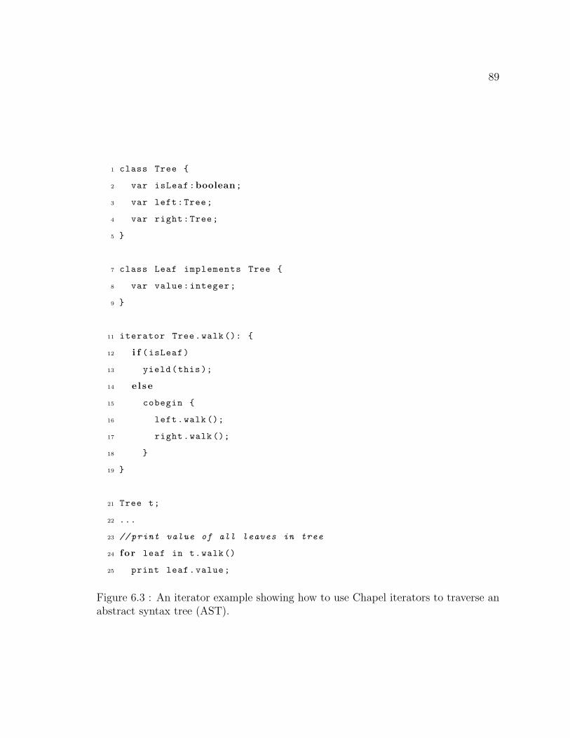
89
1 class Tree {
2 var isLeaf:boolean;
3 var left:Tree;
4 var right:Tree;
5 }
7 class Leaf implements Tree {
8 var value:integer;
9 }
11 iterator Tree.walk (): {
12 i f (isLeaf)
13 yield(this);
14 e l se
15 cobegin {
16 left.walk ();
17 right.walk ();
18 }
19 }
21 Tree t;
22 ...
23 //print value of all leaves in tree
24 for leaf in t.walk()
25 print leaf.value;
Figure 6.3 : An iterator example showing how to use Chapel iterators to traverse anabstract syntax tree (AST).
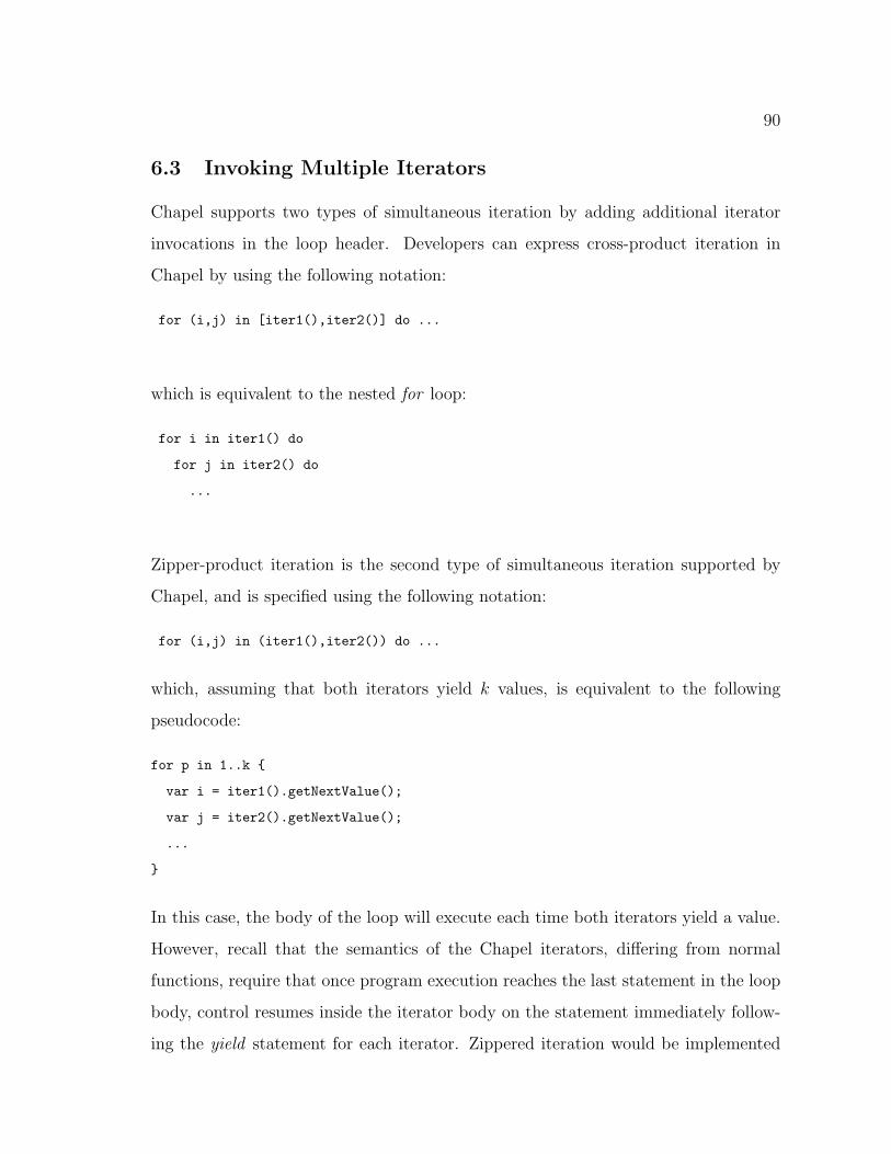
90
6.3 Invoking Multiple Iterators
Chapel supports two types of simultaneous iteration by adding additional iterator
invocations in the loop header. Developers can express cross-product iteration in
Chapel by using the following notation:
for (i,j) in [iter1(),iter2()] do ...
which is equivalent to the nested for loop:
for i in iter1() do
for j in iter2() do
...
Zipper-product iteration is the second type of simultaneous iteration supported by
Chapel, and is specified using the following notation:
for (i,j) in (iter1(),iter2()) do ...
which, assuming that both iterators yield k values, is equivalent to the following
pseudocode:
for p in 1..k {
var i = iter1().getNextValue();
var j = iter2().getNextValue();
...
}
In this case, the body of the loop will execute each time both iterators yield a value.
However, recall that the semantics of the Chapel iterators, differing from normal
functions, require that once program execution reaches the last statement in the loop
body, control resumes inside the iterator body on the statement immediately follow-
ing the yield statement for each iterator. Zippered iteration would be implemented

91
naturally using coroutines [48], which allow for execution to begin anywhere inside of
a function, unlike functions in most current languages. However, without coroutines,
zipper-product iteration may still be implemented using techniques we describe in
Section 6.5.
6.4 Implementation Techniques
Chapel has two iterator implementation techniques, an iterator approach using se-
quences and an alternate approach using nested functions. The original approach
was the sequence based implementation. Our contribution to Chapel iterators is the
nested function based implementation. The motivation for our nested function based
approach was to overcome the limitations of the sequence based approach. In the
next sections we first describe the original Chapel iterator implementation and sub-
sequently introduce our nested-function based solution to address the limitations of
the original technique.
6.4.1 Sequence Implementation
The Chapel compiler’s original implementation approach for iterators uses sequences
to store the iteration space of the data structures traversed by the loop. Subsequently,
the loop body is executed once for each element in the sequence.
Sequences in Chapel are homogeneous lists which support iteration via a built-in
iterator. Chapel supports declarations of sequence variables and iterations over them
using the following syntax:
var aseq: seq(integer) = (/ 1, 2, 4 /);
for myInt in aseq do ...
where integer in this example can be replaced by any type.
In the sequence-based implementation, Chapel first evaluates the iterator call and
builds up the sequence of yielded values before executing the loop body. Each time

92
1 // Illustration of compiler transformation
2 function tiledcmo(d1,d2): seq(2* integer) {
3 var resultSeq: seq(2* integer );
4 var (b1 ,b2) = computeTileSizes ();
5 for j in 1..d2 by b2 do
6 for i in 1..d1 by b1 do
7 for jj in j..min(d2 ,j+(b2 -1)) do
8 for ii in i..min(d1 ,i+(b1 -1)) do
9 resultSeq.append(ii,jj);
10 return resultSeq;
11 }
13 function evolve(d1,d2) {
14 var resultSeq = tiledcmo(d1 ,d2);
15 for (i,j) in resultSeq {
16 u0(i,j) = u0(i,j)* twiddle(i,j);
17 u1(i,j) = u0(i,j);
18 }
19 }
Figure 6.4 : An implementation of tiled iteration using the sequence-based approach.
the iterator yields a value, instead of executing the loop body, Chapel appends the
value to a sequence. When execution reaches either the end of the iterator or a return
statement, the iterator returns the constructed sequence of yielded values. Once the
iterator returns its sequence of values, Chapel begins executing the loop body once
for each element in the sequence returned from the iterator. Figure 6.4 illustrates the
compiler rewrite that would take place using the sequence-based iteration approach
for the tiled iterator of Figure 6.1.
The advantage to using the original approach is its simplicity. The Chapel com-
piler can use the language’s built-in support for sequences to capture the iteration

93
space and to control how many times the loop body executes. Another advantage is
that the iterator function only needs to be called once. As a result, this approach
saves the cost of transferring control back and forth between the iterator and the loop
body.
The chief disadvantage to this approach is that it is not general. It can only be
applied when the compiler can ensure that no side effects exist between the iterator
and loop body. Chapel must impose the side effect restriction because the sequence
gathers the iteration space before loop body execution begins. If there was a side effect
inside the loop body, such as changing the bounds of the iteration space, incorrect
code could be produced. A second disadvantage to this approach is the space overhead
required to store the sequence. The next section details our nested function-based
Chapel iterator implementation approach, which addresses these limitations.
6.4.2 Nested Function Implementation
Our novel contribution to the Chapel compiler is the alternative iterator implemen-
tation strategy using nested functions [59]. Currently, this approach works well on a
for loop containing one iterator call in its loop header. We provide insight on extend-
ing this approach to handle zipper-product iteration in Section 6.5. Implementing
zipper-product iteration is a subject for future work.
There are two steps to implementing Chapel iterators with nested functions. The
first step involves creating a nested function within the iterator’s scope that imple-
ments the for loop’s body and takes the loop indices as its arguments. The second
step creates a copy of the iterator, converting it to a function and replacing each
yield statement in the body with a call to the nested function created during the first
step. The transformation passes the value of each yield statement as arguments to
the nested function. Once the transformation completes this process, it replaces the
original for loop with the cloned iterator call, previously located in its loop header.
Figure 6.5 demonstrates how the Chapel compiler implements iterators using nested

94
1 // Illustration of compiler transform
2 function evolve(d1,d2) {
3 function tiledcmo(d1,d2) {
4 function loopbody(i,j) {
5 u0(i,j) = u0(i,j)* twiddle(i,j);
6 u1(i,j) = u0(i,j);
7 }
8 var (b1 ,b2) = computeTileSizes ();
9 for j in 1..d2 by b2 do
10 for i in 1..d1 by b1 do
11 for jj in j..min(d2 ,j+(b2 -1)) do
12 for ii in i..min(d1 ,i+(b1 -1)) do
13 loopbody(ii,jj);
14 }
15 tiledcmo(d1,d2);
16 }
Figure 6.5 : An implementation of tiled iteration using the nested function-basedapproach.
95
functions for the tiling example.
Since the body of the nested function inside the iterator is small, it is often
beneficial to inline it. Chapel inlines the nested function calls appearing inside the
iterator to eliminate the costs of invoking the nested function every time the iterator
yields a value. This optimization is not possible with the sequence-based approach
since the iterator must yield all its values before preceding to execute the loop body.
Another advantage of using the nested function approach for iterators is generality:
side effects between the iterator and the for loop’s body do not have to be identified in
fear of producing incorrect code. As a result, this approach is more broadly applicable
than using the sequence-based approach. The execution behavior of this approach
is closer to that of CLU [69] and Sather [76] iterators. In addition, an advantage
over the sequence-based approach is Chapel does not need to use storage for the
iteration space. Consequently, the nested-function implementation is more practical
in environments where large iteration spaces may be in danger of overflowing memory.
6.5 Zippered Iteration
Zipper-product iteration is the process of traversing through multiple iterators si-
multaneously where each iterator must yield a value once before execution of the
loop body can begin. Figure 6.6 shows an example of zippered iteration in Chapel.
This section describes possible zipper-product implementation approaches that we
are exploring as we go forward. Chapel’s semantics define that zippered iteration
is performed by requiring the iterators involved in the loop to each yield values be-
fore the loop body is executed. Recall that semantically, when an iterator yields a
value, execution suspends from inside the iterator until the loop body has completed
once. When execution resumes inside the iterator, Chapel will execute the statement
immediately following the yield statement.
In modern languages, the only point of entry for functions is at the top. Coroutines
are functions that can have multiple entry points and properly simulate the producer/-

96
1 iterator fibonacci(n): integer {
2 var i1 = 0, i2 = 1;
3 var i = 0;
4 while i <= n {
5 yield i1;
6 var i3 = i1 + i2;
7 i1 = i2;
8 i2 = i3;
9 i += 1;
10 }
11 }
13 iterator squares(n): integer {
14 var i = 0;
15 while i <= n {
16 yield i * i;
17 i += 1;
18 }
19 }
21 for i, j in fibonacci (12), squares (12) do
22 writeln(i, ", ", j);
Figure 6.6 : An example of zippered iteration in Chapel.

97
consumer relationship that simultaneous iteration between two iterators introduces.
However, because most modern languages do not support coroutines, programmers
must utilize other methods to properly simulate the producer/consumer relationship.
Here we consider two techniques, one that uses state variables and one that uses
multiple threads via synchronization variables.
Figure 6.7 shows one technique for implementing zipper-product iteration. The
example implements the zippered iteration using state variables. Both iterators use
Chapel’s select statement with goto statements to enable simulation of a coroutine,
similar to checkpointing in the porch compiler [92]. The state is preserved via the class
that is passed into the function. The semantic execution behavior of the iterators is
preserved by ensuring that the statement immediately following the yield is executed
when the iterators are invoked on subsequent calls. Once the last yield is executed,
the iterator will not be called again. The advantage of using this approach is that
it eliminates the synchronization costs that are associated with our second approach.
Also, by having the compiler simulate the coroutine, dead variables do not need to
have their state saved. For example, an optimization could be performed to eliminate
i3 from the state class for the Fibonacci iterator. The disadvantage of this approach
is the overhead associated with entering and exiting the routine. This could be
especially significant in recursive iterators where the stack would result in a large
saved state class.
Our second implementation approach for zippered iteration uses multiple threads
and synchronization (sync) variables. A sync variable[34] transitions to an undefined
state when read. When a sync variable is undefined and a computation tries to read
from it, the computation will stall until the sync variable is defined. As a result, sync
variables allow us to model the producer/consumer relationship of coroutines that is
needed to support zippered iteration. Note that the multi-threaded solution requires
analysis which determines whether the iterators are parallel-safe or semantics which
imply that iterators in a zippered context are executed in parallel.
98
In Figure 6.8, the sync variables are initially undefined. Each sync variable can
transition to the defined state inside an iterator. Chapel utilizes the cobegin statement
to indicate that both iterators should be executed in parallel. The while loop inside
the cobegin statement will stall until each iterator defines its sync variables. A sync
variable is created for each iterator and a sync variable assignment replaces each yield
statement inside the iterator. The chief disadvantage to using this approach lies in
the synchronization costs associated with the sync variables. Both approaches enable
the support of zippered iteration in Chapel.

99
1 // Illustration of compiler transform
2 class ss_fib_state {var i1,i2,i3, i:integer; var jump = 1;}
3 function ss_fibonacci(n, ss): integer {
4 select ss.jump {when 1 do goto lab1; when 2 do goto lab2;}
5 label lab1 ss.i1 = 0;
6 ss.i2 = 1; ss.i = 0;
7 while ss.i <= n {
8 ss.jump = 2;
9 return ss.i1;
10 label lab2 ss.i3 = ss.i1 + ss.i2;
11 ss.i1 = ss.i2; ss.i2 = ss.i3;
12 ss.i += 1; }
13 ss.jump = 0;
14 return 0;
15 }
16 class ss_sq_state { var i:integer; var jump = 1; }
17 function ss_squares(n, ss): integer {
18 select ss.jump {when 1 do goto lab1; when 2 do goto lab2;}
19 label lab1 ss.i = 0;
20 while ss.i <= n {
21 ss.jump = 2;
22 return ss.i * ss.i;
23 label lab2 ss.i += 1; }
24 ss.jump = 0;
25 return 0;
26 }
27 var ss1 = ss_fib_state (); var ss2 = ss_sq_state ();
28 while ss1.jump and ss2.jump do {
29 var i = ss_fibonacci (12, ss1); var j = ss_squares (12, ss2);
30 writeln(i, ", ", j);
31 }
Figure 6.7 : An implementation of zippered iteration using state variables.

100
1 // Illustration of compiler transform
2 class mt_fib_state{sync flag:bool; sync result:integer ;}
3 function mt_fibonacci(n, mt) {
4 var i1 = 0, i2 = 1, i = 0;
5 while i <= n {
6 mt.flag = f a l s e ;
7 mt.result = i1;
8 var i3 = i1 + i2;
9 i1 = i2;
10 i2 = i3;
11 i += 1; }
12 mt.flag = true;
13 }
14 class mt_sq_state{sync flag:bool; sync result:integer ;}
15 function mt_squares(n, mt) {
16 var i = 0;
17 while i <= n {
18 mt.flag = f a l s e ;
19 mt.result = i * i;
20 i += 1; }
21 mt.flag = true;
22 }
23 var mt1 = mt_fib_state (); var mt2 = mt_sq_state ();
24 cobegin {
25 mt_fibonacci (12);
26 mt_squares (12);
27 while not mt1.flag and not mt2.flag do
28 writeln(mt1.result , ", ", mt2.result );
29 }
Figure 6.8 : A multi-threaded implementation of zippered iteration using sync vari-ables.

101
Chapter 7
Performance Results
We ran the first set of experiments on a 1.25 GHz PowerPC G4 with 1.5 GB of
memory using the Sun Java Hotspot VM (build 1.5.0 07-87) for Java 5. We measured
performance results on the Java Grande benchmarks written in X10. These results are
obtained using the class A versions of the benchmark. We report results for 3 different
versions of the benchmark suite. Version 1 is an unoptimized direct translation of the
original Java version obtained from the Java Grande Forum web site [54] renamed
with the .x10 extension, with all Java arrays converted into X10 arrays and integer
subscripts replaced by points. Version 2 uses the same input X10 program as in
Version 1 but turns on point inlining and uses programmer inserted dependent types
to improve performance. Version 3, containing only Java arrays, can be considered as
the baseline. We refer to Version 3 as X10 Light. These results include runtime array
bounds checks, null pointer checks and other checks associated with a Java runtime
environment.
Table 7.1 shows the impact unoptimized high-level X10 array computation has on
performance by comparing Versions 1 and 3. The unoptimized X10 version runs up
to almost 84 times slower. Table 7.2 shows the impact of the inlining points and gen-
erating efficient array accesses with dependent types by comparing the performance
of Versions 1 and 2. While performance improvements in the range of 1.6× to 5.4×
were observed for 7 of 8 benchmarks in Table 7.2, there still remain opportunities
to employ automatic compiler interprocedural rank inference to replace high-level
X10 arrays with more efficient representations; thereby leading to even better per-
formance. Note: we observed no improvement in the series benchmark because its

102
performance is dominated by scalar (rather than array) operations.
Benchmarks Sequential Runtime Performance in seconds Performance Slowdown
Unopt. X10 (Version 1) X10 Light (Version 3) (Version 3)/(Version 1)
sparsematmult 57.97 9.75 5.95
crypt 8.14 4.60 1.77
lufact 52.87 1.38 38.31
sor 508.49 6.06 83.91
series 19.01 19.01 1.00
moldyn 2.39 0.57 4.19
montecarlo 7.59 3.00 2.53
raytracer 2.27 1.28 1.77
Table 7.1 : Raw runtime performance showing slowdown that results from not opti-mizing points and high-level arrays in sequential X10 version of Java Grande bench-marks.
The second set of performance results reported in this section were obtained using
the following system settings:
• The target system is either an IBM 64-way 2.3 GHz Power5+ SMP with 512
GB main memory or an IBM 16-way 4.7 GHz Power6 SMP with 186 GB main
memory. Assume the former unless otherwise specified. The 16-way machine
was used for the bounds check elimination results.
• The Java runtime environment used is the IBM J9 virtual machine (build 2.4,
J2RE 1.6.0) which includes the IBM TestaRossa (TR) Just-in-Time (JIT) com-
piler [93]. The following internal TR JIT options were used for all X10 runs:
– Options to enable classes to be preloaded, and each method to be JIT-
compiled at a high (”very hot”) optimization level on its first execution.
– An option to ignore strict conformance with IEEE floating point.

103
Benchmarks Sequential Runtime Performance in seconds Speedup Factor
Unopt. X10 (Version 1) Opt. X10 (Version 2) (Version 1)/(Version 2)
sparsematmult 57.97 13.83 4.1×
crypt 8.14 4.79 1.7×
lufact 52.87 18.86 2.8×
sor 508.49 93.41 5.4×
series 19.01 18.95 1.0×
moldyn 2.39 1.19 2.0×
montecarlo 7.59 3.49 2.2×
raytracer 2.27 1.43 1.6×
Table 7.2 : Raw runtime performance from optimizing points and using dependenttypes to optimize high-level arrays in sequential X10 version of Java Grande bench-marks.
• A special skip checks option was used for some of the results to measure the
opportunities for optimization. This option directs the JIT compiler to disable
all runtime checks (array bounds, null pointer, divide by zero).
• Version 1.5 of the X10 compiler and runtime [101] were used for all executions.
This version supports implicit syntax [100] for place-remote accesses. In addi-
tion, all runs were performed with the number of places set to 1, so all runtime
“bad place” checks [25] were disabled.
• The default heap size was 2GB.
• For all runs, the main program was extended with a three-iteration loop within
the same Java process, and the best of the three times was reported in each
case. This configuration was deliberately chosen to reduce the impact of JIT
compilation time, garbage collection and other sources of perturbation in the
performance comparisons.
The benchmarks studied in the second set of experiments are X10 ports of bench-
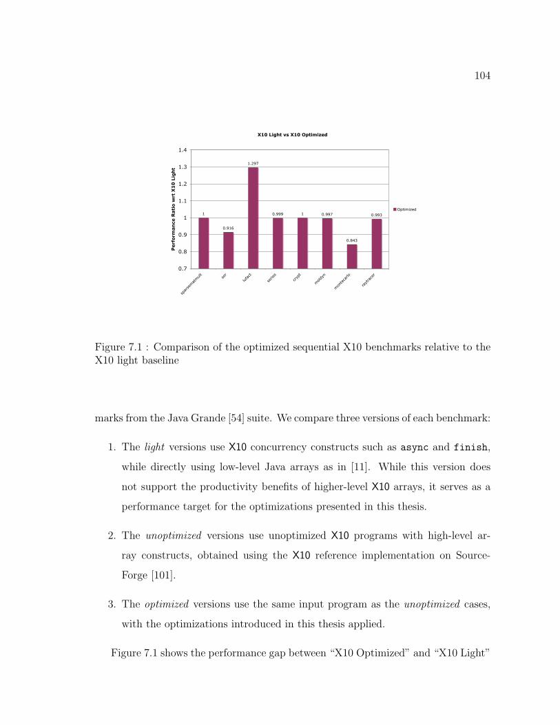
104
X10 Light vs X10 Optimized
1
0.916
1.297
0.999 1 0.997
0.843
0.993
0.7
0.8
0.9
1
1.1
1.2
1.3
1.4
sparsematmult
sor
lufact
series
crypt
moldyn
montecarlo
raytracer
Perf
orm
an
ce R
ati
o w
rt X
10
Lig
ht
Optimized
Figure 7.1 : Comparison of the optimized sequential X10 benchmarks relative to theX10 light baseline
marks from the Java Grande [54] suite. We compare three versions of each benchmark:
1. The light versions use X10 concurrency constructs such as async and finish,
while directly using low-level Java arrays as in [11]. While this version does
not support the productivity benefits of higher-level X10 arrays, it serves as a
performance target for the optimizations presented in this thesis.
2. The unoptimized versions use unoptimized X10 programs with high-level ar-
ray constructs, obtained using the X10 reference implementation on Source-
Forge [101].
3. The optimized versions use the same input program as the unoptimized cases,
with the optimizations introduced in this thesis applied.
Figure 7.1 shows the performance gap between “X10 Optimized” and “X10 Light”

105
(Version 1). The gap is at most 16% for MonteCarlo), but is under 1% in most other
cases. In Figure 7.1, the reason why “X10 Optimized” delivers better performance
than “X10 Light” for LUFact is because the address arithmetic present in the “X10
Light” version was naturally factored out in the “X10 Optimized” version due to the
use of region iterators and points. We could modify the “X10 Light” version in this
case to match the code that would be generated by the “X10 Optimized” version,
but we instead chose to be faithful to the original Java Grande Forum benchmark
structure when creating the “X10 Light” versions.
Next, we discuss the impact of our transformations on parallel performance. Ta-
ble 7.3 shows the relative scalability of the Optimized and Unoptimized X10 versions.
Since the biggest difference was observed for the sparsematmult benchmark, we use
Figure 7.2 and 7.3 to further study this behavior for sparsematmult. Figure 7.2
illustrates that the optimized sparsematmult benchmark scales better than the un-
optimized version with an initial minimum heap size of 2 GB. Figure 7.3 shows that
decreasing the initial minimum heap size to the default (4MB) value further increases
the gap in scalability, suggesting that garbage collection is a major scalability factor in
the Unoptimized case. These results are not surprising since the Unoptimized version
allocates a large number of point objects with short life times. Figures 7.4, 7.5, 7.6,
and 7.7 show, using lufact and sor, that this behavior is not limited to sparsemat-
mult. The Optimized version mitigates this problem by inlining point objects. We
demonstrate with Figures 7.8 and 7.9 that Unoptimized X10 can scale as well as
Optimized X10 in the absence of point-intensive loops. Figures 7.10, 7.11, 7.12, 7.13
provide additional examples to highlight our optimization’s scalability impact using
a minimum 2 GB heap size. Note that in all these results, the Optimized speedup
is relative to the 1-CPU optimized performance, and the Unoptimized speedup is
relative to the 1-CPU unoptimized performance.
Table 7.4 shows the raw execution times for the unoptimized and optimized ver-
sions, and Figure 7.14 shows the relative speedup obtained due to optimization as we
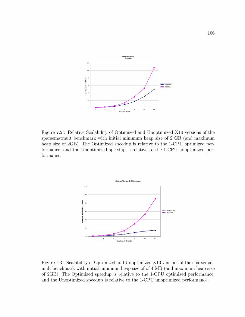
106
SparseMatmult C Speedup
0
20
40
60
80
100
120
1 2 4 8 16 32 64Number of threads
Spee
dup
rela
tive
to 1
thre
adUnoptimizedOptimized
Figure 7.2 : Relative Scalability of Optimized and Unoptimized X10 versions of thesparsematmult benchmark with initial minimum heap size of 2 GB (and maximumheap size of 2GB). The Optimized speedup is relative to the 1-CPU optimized per-formance, and the Unoptimized speedup is relative to the 1-CPU unoptimized per-formance.
SparseMatmult C Speedup
0
20
40
60
80
100
120
1 2 4 8 16 32 64
Number of threads
Sp
eed
up
rela
tive t
o 1
th
read
UnoptimizedOptimized
Figure 7.3 : Scalability of Optimized and Unoptimized X10 versions of the sparsemat-mult benchmark with initial minimum heap size of of 4 MB (and maximum heap sizeof 2GB). The Optimized speedup is relative to the 1-CPU optimized performance,and the Unoptimized speedup is relative to the 1-CPU unoptimized performance.

107
LUFact C Speedup
0
5
10
15
20
25
30
1 2 4 8 16 32 64
Number of threads
Sp
eed
up
rela
tive t
o 1
th
read
UnoptimizedOptimized
Figure 7.4 : Relative Scalability of Optimized and Unoptimized X10 versions of thelufact benchmark with initial minimum heap size of 2 GB (and maximum heap sizeof 2GB). The Optimized speedup is relative to the 1-CPU optimized performance,and the Unoptimized speedup is relative to the 1-CPU unoptimized performance.
LUFact C Speedup
0
2
4
6
8
10
12
1 2 4 8 16 32 64Number of threads
Spee
dup
rela
tive
to 1
thre
ad
UnoptimizedOptimized
Figure 7.5 : Scalability of Optimized and Unoptimized X10 versions of the lufactbenchmark with initial minimum heap size of of 4 MB (and maximum heap size of2GB). The Optimized speedup is relative to the 1-CPU optimized performance, andthe Unoptimized speedup is relative to the 1-CPU unoptimized performance.

108
SOR C Speedup
0
5
10
15
20
25
30
1 2 4 8 16 32 64
Number of threads
Sp
eed
up
rela
tive t
o 1
th
read
UnoptimizedOptimized
Figure 7.6 : Relative Scalability of Optimized and Unoptimized X10 versions of thesor benchmark with initial minimum heap size of 2 GB (and maximum heap size of2GB). The Optimized speedup is relative to the 1-CPU optimized performance, andthe Unoptimized speedup is relative to the 1-CPU unoptimized performance.
SOR C Speedup
0
1
2
3
4
5
6
7
8
9
10
1 2 4 8 16 32 64Number of threads
Spee
dup
rela
tive
to 1
thre
ad
UnoptimizedOptimized
Figure 7.7 : Scalability of Optimized and Unoptimized X10 versions of the sor bench-mark with initial minimum heap size of of 4 MB (and maximum heap size of 2GB).The Optimized speedup is relative to the 1-CPU optimized performance, and theUnoptimized speedup is relative to the 1-CPU unoptimized performance.

109
Series C Speedup
0
5
10
15
20
25
30
35
1 2 4 8 16 32 64
Number of threads
Sp
eed
up
rela
tive t
o 1
th
read
UnoptimizedOptimized
Figure 7.8 : Relative Scalability of Optimized and Unoptimized X10 versions of theseries benchmark with initial minimum heap size of 2 GB (and maximum heap size of2GB). The Optimized speedup is relative to the 1-CPU optimized performance, andthe Unoptimized speedup is relative to the 1-CPU unoptimized performance.
Series C Speedup
0
5
10
15
20
25
30
35
1 2 4 8 16 32 64Number of threads
Spee
dup
rela
tive
to 1
thre
ad
UnoptimizedOptimized
Figure 7.9 : Scalability of Optimized and Unoptimized X10 versions of the seriesbenchmark with initial minimum heap size of of 4 MB (and maximum heap size of2GB). The Optimized speedup is relative to the 1-CPU optimized performance, andthe Unoptimized speedup is relative to the 1-CPU unoptimized performance.
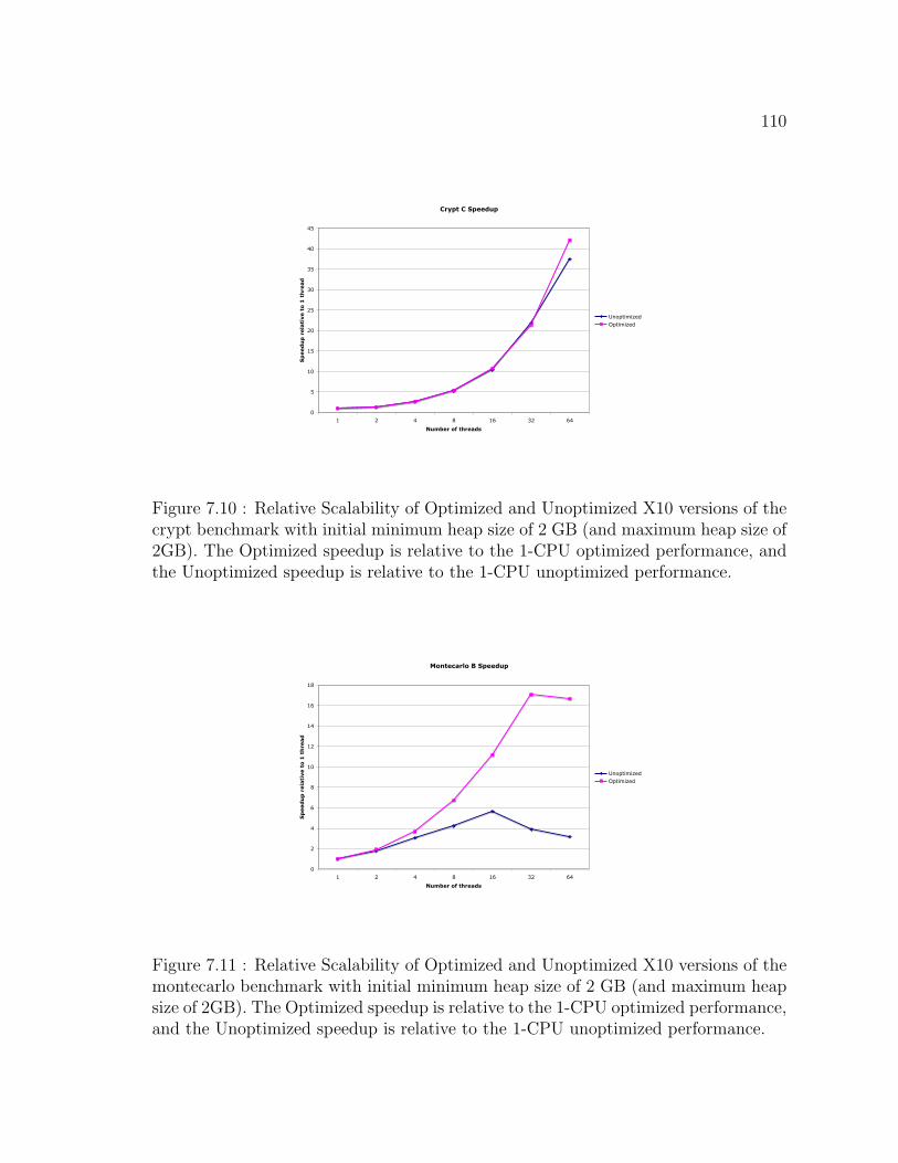
110
Crypt C Speedup
0
5
10
15
20
25
30
35
40
45
1 2 4 8 16 32 64
Number of threads
Sp
eed
up
rela
tive t
o 1
th
read
UnoptimizedOptimized
Figure 7.10 : Relative Scalability of Optimized and Unoptimized X10 versions of thecrypt benchmark with initial minimum heap size of 2 GB (and maximum heap size of2GB). The Optimized speedup is relative to the 1-CPU optimized performance, andthe Unoptimized speedup is relative to the 1-CPU unoptimized performance.
Montecarlo B Speedup
0
2
4
6
8
10
12
14
16
18
1 2 4 8 16 32 64
Number of threads
Sp
eed
up
rela
tive t
o 1
th
read
UnoptimizedOptimized
Figure 7.11 : Relative Scalability of Optimized and Unoptimized X10 versions of themontecarlo benchmark with initial minimum heap size of 2 GB (and maximum heapsize of 2GB). The Optimized speedup is relative to the 1-CPU optimized performance,and the Unoptimized speedup is relative to the 1-CPU unoptimized performance.
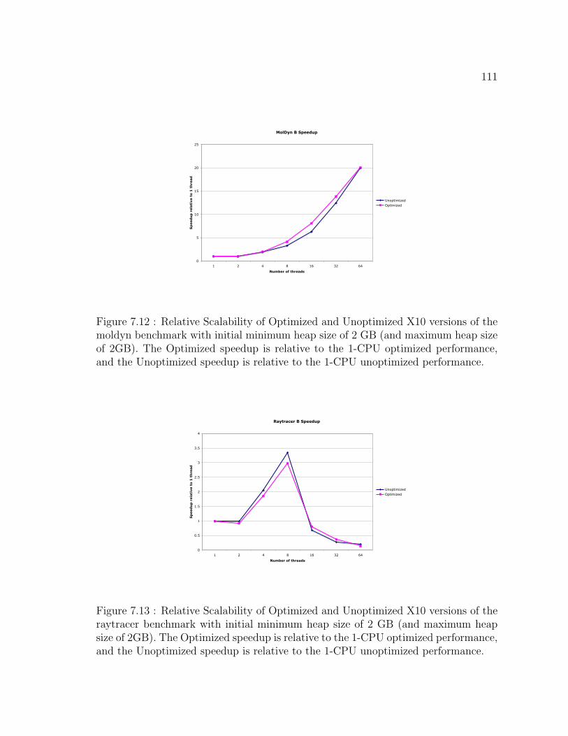
111
MolDyn B Speedup
0
5
10
15
20
25
1 2 4 8 16 32 64
Number of threads
Sp
eed
up
rela
tive t
o 1
th
read
UnoptimizedOptimized
Figure 7.12 : Relative Scalability of Optimized and Unoptimized X10 versions of themoldyn benchmark with initial minimum heap size of 2 GB (and maximum heap sizeof 2GB). The Optimized speedup is relative to the 1-CPU optimized performance,and the Unoptimized speedup is relative to the 1-CPU unoptimized performance.
Raytracer B Speedup
0
0.5
1
1.5
2
2.5
3
3.5
4
1 2 4 8 16 32 64
Number of threads
Sp
eed
up
rela
tive t
o 1
th
read
UnoptimizedOptimized
Figure 7.13 : Relative Scalability of Optimized and Unoptimized X10 versions of theraytracer benchmark with initial minimum heap size of 2 GB (and maximum heapsize of 2GB). The Optimized speedup is relative to the 1-CPU optimized performance,and the Unoptimized speedup is relative to the 1-CPU unoptimized performance.

112
X10 Unoptimized vs X10 Optimized
0
50
100
150
200
250
300
1 2 4 8 16 32 64
Number of threads
X1
0 U
no
pti
miz
ed
/ X
10
Op
tim
ized
SparseMatmult:SizeCSOR:SizeCLUFact:SizeCSeries:SizeCCrypt:SizeCMolDyn:SizeBMonteCarlo:SizeBRayTracer:SizeB
Figure 7.14 : Speedup of Optimized X10 version relative to Unoptimized X10 version.
scale from 1 to 64 CPUs. Figure 7.15 zooms in on Figure 7.14. As can be seen in
Table 7.4 and Figure 7.14, the performance improvements due to optimization can be
very significant, reaching as a high as a factor of 266×. The reason “series” behaves
differently in Table 7.4 is due to the fact that its frequently-executed code regions
are dominated by scalar computations. As a result, our array optimizations have
very limited opportunities to impact performance for this benchmark. However, as
shown in Table 7.4, the optimization opportunities are much larger for other scientific
applications that are array intensive (as is the norm).
The benchmarks studied in the next set of experiments are X10 sequential ports
of benchmarks from the Java Grande [54] suite. We compare two versions of each
benchmark. The first version is the ported code. The second version, through static
analysis, inserts noBoundsCheck calls around an array index when the bounds check
is unnecessary.

113
X10 Unoptimized vs X10 Optimized
0
2
4
6
8
10
12
14
16
18
1 2 4 8 16 32 64
Number of threads
X1
0 U
no
pti
miz
ed
/ X
10
Op
tim
ized
Series:SizeCCrypt:SizeCMolDyn:SizeBMonteCarlo:SizeBRayTracer:SizeB
Figure 7.15 : Speedup of Optimized X10 version relative to Unoptimized X10 version(zoom in of Figure 7.14).
Benchmarks Runtime Performance speedup (relative to 1 CPUs)
(unopt/opt) 1 2 4 8 16 32 64
sparsemm 1.0/1.0 2.2/2.5 4.2/5.9 9.0/13.5 16.9/29.6 30.6/52.3 49.1/107.4
crypt 1.0/1.0 1.3/1.4 2.6/2.7 5.3/5.4 10.4/10.8 21.8/21.4 37.5/42.2
lufact 1.0/1.0 1.9/2.2 3.9/4.4 7.4/8.5 13.7/15.8 22.2/24.9 25.2/18.7
sor 1.0/1.0 1.9/2.2 3.9/4.5 7.5/8.6 13.8/14.9 21.9/20.0 25.8/14.5
series 1.0/1.0 1.0/1.0 2.1/2.1 4.1/4.1 8.2/8.2 16.2/16.4 32.5/32.8
moldyn 1.0/1.0 1.1/1.0 1.9/2.0 3.3/4.1 6.3/8.2 12.5/13.9 20.0/20.1
montecarlo 1.0/1.0 1.8/1.9 3.1/3.7 4.2/6.7 5.7/11.2 3.9/17.1 3.2/16.7
raytracer 1.0/1.0 1.0/0.9 2.1/1.9 3.4/3.0 0.7/0.8 0.3/0.4 0.2/0.1
Table 7.3 : Relative Scalability of Optimized and Unoptimized X10 versions with heapsize of 2 GB. The Optimized speedup is relative to the 1-CPU optimized performance,and the Unoptimized speedup is relative to the 1-CPU unoptimized performance. TheOptimized X10 version does not include the bounds check optimization.

114
Benchmarks Runtime Performance (scaling from 1 to 64 CPUs) in seconds
(unopt/opt) 1 2 4 8 16 32 64
sparsemm 309.5/13.5 138.7/5.4 74.0/2.3 34.3/1.0 18.3/0.5 10.1/0.3 6.3/0.1
crypt 36.4/7.7 28.2/5.7 13.9/2.9 6.9/1.4 3.5/0.7 1.7/0.4 1.0/0.2
lufact 937.1/5.2 496.6/2.5 238.5/1.2 126.3/0.7 68.5/0.4 42.2/0.2 37.3/0.3
sor 614.3/2.8 332.9/1.3 157.8/0.6 81.9/0.3 44.7/0.2 28.0/0.1 23.8/0.2
series 1766.1/1764.9 1767.1/1764.6 851.0/850.7 429.0/429.0 215.2/215.1 108.9/107.7 54.4/53.8
moldyn 199.9/56.3 179.9/57.6 102.9/28.0 60.5/13.7 31.8/6.9 16.0/4.1 10.0/2.8
montecarlo 76.4/26.0 42.5/13.4 24.9/7.1 18.1/3.9 13.5/2.3 19.6/1.5 24.0/1.6
raytracer 203.9/115.3 206.4/124.8 99.1/62.1 60.8/38.7 297.4/141.8 735.0/312.8 985.8/804.0
Table 7.4 : Raw runtime performance of Unoptimized and Optimized X10 versions aswe scale from 1 to 64 CPUs. The Optimized X10 version does not include the boundscheck optimization.
In Table 7.5, we report the dynamic counts for the Java Grande, hexahedral, and
2 NAS parallel (cg, mg) X10 benchmarks. We compare dynamic counts for potential
general X10 array bounds checks against omitted general X10 array bounds checks
using our static analysis techniques. We use the term ”general X10 array” to refer to
arrays the programmer declares using X10 regions. In several cases our static bounds
analysis removes over 99% of potential bound checks.
In Figure 7.16, we report the execution times for the Java Grande, hexahedral,
and 2 NAS parallel (cg, mg) X10 benchmarks both with and without the automat-
ically generated noBoundsCheck annotations with runtime checks enabled. These
annotations alert the IBM J9 VM when array bounds checking for an array access is
unnecessary. Performing static array bounds analysis and subsequent automatic pro-
gram transformation, we increase runtime performance by up to 22.3%. These results
demonstrate that our static no bounds check analysis helps reduce the performance
impact of programmers developing applications in type-safe languages. Table 7.6
shows that we may further improve runtime performance in some cases by eliminat-
ing other types of runtime checks such as null checks and cast checks.
Finally, in Table 7.7, we compare Fortran, Unoptimized X10, Optimized X10, and

115
Java execution times for the 2 NAS parallel (cg, mg) benchmarks. The Optimized X10
significantly reduces the slowdown factor that results from comparing Unoptimized
X10 with Fortran. These results were obtained on the IBM 16-way SMP. Note: the
3.0 NAS Java mg version was run on a 2.16 GHz Intel Core 2 Duo with 2GB of
memory due to a J9 JIT compilation problem with this code version. In the future,
we will continue to extend our optimizations to further reduce the overhead of using
high-level X10 array computations.
Benchmarks Dynamic Counts for X10 Array Bounds Checks (ABCs)
total X10 total X10 percent
ABCs ABCs eliminated eliminated
sparsemm 2,513,000,000 2,513,000,000 100.0%
crypt 1,000,000,312 100,000,130 10.0%
lufact 5,425,377,953 5,375,370,956 99.1%
sor 4,806,388,808 4,798,388,808 99.8%
series 4,000,020 4,000,002 99.9%
moldyn 5,955,209,518 4,023,782,878 67.6%
montecarlo 779,845,962 419,887,788 53.8%
raytracer 1,185,054,651 1,185,054,651 100.0%
hexahedral 35,864,066,928 32,066,331,077 89.4%
cg 3,044,164,220 1,532,754,859 50.4%
mg 6,614,097,502 383,155,390 5.8%
Table 7.5 : Dynamic counts for the total number of X10 array bounds checks (ABC)in sequential JavaGrande, hexahedral benchmark and 2 NAS Parallel X10 benchmarkscompared with the total number of eliminated checks we introduce using static com-piler analysis and compiler annotations which signal the JVM to remove unnecessarybounds checks.

116
Performance Improvement over X10 Light
-5%
0%
5%
10%
15%
20%
25%
sparsemmcrypt
lufact so
r
series
moldyn
montecarlo
raytracer
hexahedral cg m
g
Figure 7.16 : Comparison of the X10 light baseline to the optimized sequential X10benchmarks with compiler inserted annotations used to signal the VM when to elim-inate bounds checks.

117
Benchmarks Sequential Runtime Performance in seconds
skip runtime runtime runtime checks + runtime
checks checks compiler annotations improvement
sparsemm 24.01 34.46 27.02 21.6%
crypt 8.79 9.10 9.11 0.1%
lufact 39.59 46.86 40.43 13.7%
sor 3.66 3.67 3.66 0.2%
series 1218.39 1233.77 1226.61 0.6%
moldyn 75.21 89.98 88.65 1.5%
montecarlo 24.19 24.64 24.41 0.9%
raytracer 33.11 34.79 35.73 -2.4%
hexahedral 10.38 15.31 12.03 22.3%
cg 9.04 9.73 9.34 4.0%
mg 29.39 31.30 30.40 2.9%
Table 7.6 : Raw sequential runtime performance of JavaGrande and 2 NAS ParallelX10 benchmarks with static compiler analysis to signal the JVM to eliminate unnec-essary array bounds checks. These results were obtained on the IBM 16-way SMPbecause the J9 VM has the special option to eliminate individual bounds checks whendirected by the compiler.
Benchmarks Sequential Runtime Performance
Fortran Unopt. X10 Slowdown Opt. X10 Slowdown Java Slowdown
Version Version Factor Version Factor Version Factor
cg 2.58 26.9 10.43× 8.54 3.31× 4.14 1.60×
mg 2.02 94.37 46.72× 27.59 13.66× 19.25 9.53×
Table 7.7 : Fortran, Unoptimized X10, Optimized X10, and Java raw sequentialruntime performance comparison (in seconds) for 2 NAS Parallel benchmarks (cg,mg). These results were obtained on the IBM 16-way SMP machine.

118
Chapter 8
Conclusions and Future Work
Although runtime performance has suffered in the past when scientists used high pro-
ductivity languages with high-level array accesses, our thesis is that these overheads
can be mitigated by compiler optimizations, thereby enabling scientists to develop
code with both high productivity and high performance. The optimizations intro-
duced in this dissertation for high-level array accesses in X10 result in performance
that rivals the performance of hand-tuned code with explicit rank-specific loops and
lower-level array accesses, and is up to two orders of magnitude faster than unopti-
mized, high-level X10 programs.
In this thesis, we discussed the Point abstraction in high-productivity languages,
and described compiler optimizations that reduce their performance overhead. We
conducted experiments that validate the effectiveness of our Point inlining optimiza-
tion combined with programmer specified dependent types and demonstrate that
these optimizations can enable high-level X10 array accesses written with implicit
ranks and Points to achieve performance comparable to that of low-level programs
written with explicit ranks and integer indices. The experimental results showed per-
formance improvements in the range of 1.6× to 5.4× for 7 of 8 Java Grande benchmark
programs written in X10, as a result of these optimizations.
This thesis provides an algorithm to generate rank-specific efficient array compu-
tations from applications that use productive rank-independent general X10 arrays.
The algorithm propagates X10 array rank information to generate the more efficient
Java arrays with precise ranks. Our results demonstrate that we can generate effi-
cient array representations and come within 84% of the baseline for each benchmark

119
and within 99% in most cases. This thesis introduces novel contributions to array
bounds analysis by taking advantage of the X10 region language abstraction along
with tracking array value ranges. We introduce an interprocedural static elimination
bounds analysis algorithm with algebraic region inequality equations for points and
integrals to establish region and sub region relationships; thereby aiding in the dis-
covery of superfluous bounds checks when programmers utilized these variables in an
array subscript or during region construction. We illustrate the benefits of array value
ranges which are particularly useful in applications with sparse matrix computations.
Experimental results show we experience runtime execution improvements of up to
22.3%. Our dynamic counts illustrate the elimination of over 99% of bounds checks
in several cases with this optimization. In addition, we provide an optimization that
provides a way to generate efficient array computations in the presence of array views
resulting in a factor of 7 speedup. Another contribution is the analysis of how our op-
timizations impact scalability. The optimized version of the benchmarks scales much
better than the unoptimized general X10 array version.
We also calibrated the performance of our optimizations for the two benchmarks
for which equivalent Fortran programs were available, CG and MG. For CG, we
improved the performance of the Unoptimized X10 by 3.15 × but there still remains
a performance gap of 3.3× relative to the Fortran version. For MG, we improved the
performance of the Unoptimized X10 by 3.42× but there still remains a performance
gap of 13.66× relative to the Fortran version. In both cases, a large part of the
performance gap can be attributed to the differences between the Java version and
the Fortran version that have been studied in past work [75]. The remainder of
the performance gap can be attributed to the cases where our optimization was not
able to convert X10 arrays to Java arrays. These cases are challenging because the
Java version includes hand-coded redundancy elimination that will require advanced
compiler techniques such as redundancy elimination [21, 30] of array accesses through
loop carried dependences to enable them to be performed automatically.

120
This thesis shows that Chapel iterators can effectively separate the specification
of an algorithm from its implementation, thereby enabling programmers to easily
switch between different specifications while also allowing them to focus on the al-
gorithm’s implementation. Using iterators to handle specifications such as iteration
space ordering allows programmers to reuse specifications instead of having to write
a specification for an algorithm each time the programmer implements an algorithm.
We describe a novel strategy we have implemented in the Chapel compiler to sup-
port Chapel iterators which addresses the limitations of the original strategy. The
first approach was sequence-based Chapel iterators and the second approach was to
implement Chapel iterators with nested functions. The second strategy eliminates
some of the imposed restrictions and spatial overhead of the first strategy.
In the future, we plan to extend our bounds analysis to discover sub region rela-
tionships between array views and to identify when regions share equivalent dimen-
sions to reduce the cost for a multi-dimensional array access. We plan to extend
array value range analysis with alias analysis to update array alias value ranges. We
also plan to analyze and potentially eliminate other types of runtime checks such as
cast checks and null checks. In addition, as part of the Habanero multicore software
research project at Rice University [50], we plan to demonstrate on a wide range
of applications that the techniques presented in this thesis can enable programmers
to develop high productivity array computations without incurring the additional
runtime costs that is usually associated with utilizing higher level language abstrac-
tions. Overall, these results emphasize the importance of the optimizations we have
presented in this thesis as a step towards achieving high performance for high pro-
ductivity languages.

121
Bibliography
[1] O. Agesen and U. Holzle. Type Feedback vs. Concrete Type Inference: A Comparison
of Optimization Techniques for Object-Oriented Languages. In OOPSLA ’95: Pro-
ceedings of the Tenth Annual Conference on Object-Oriented Programming Systems,
Languages, and Applications, pages 91–107, 1995.
[2] A. Aggarwal and K. H. Randall. Related field analysis. In PLDI ’01: Proceedings
of the ACM SIGPLAN 2001 conference on Programming language design and imple-
mentation, pages 214–220, 2001.
[3] E. Allen, D. Chase, V. Luchangco, J. Maessen, S. Ryu, G. Steele, and S. Tobin-
Hochstadt. Fortress Specification (version 1.0). Sun Microsystems Inc., Mar. 2008.
[4] G. Almasi and D. Padua. Majic: compiling matlab for speed and responsiveness.
In PLDI ’02: Proceedings of the ACM SIGPLAN 2002 Conference on Programming
language design and implementation, pages 294–303, 2002.
[5] B. Alpern, M. Butrico, A. Cocchi, J. Dolby, S. J. Fink, D. Grove, and T. Ngo.
Experiences porting the jikes rvm to linux/ia32. In Proceedings of the 2nd Java TM
Virtual Machine Research and Technology Symposium, pages 51–64, 2002.
[6] B. Alpern, M. N. Wegman, and F. K. Zadeck. Detecting equality of variables in pro-
grams. In POPL ’88: Proceedings of the 15th ACM SIGPLAN-SIGACT symposium
on Principles of programming languages, pages 1–11, New York, NY, USA, 1988.
ACM Press.
[7] J. W. Backus and W. Heising. Fortran. In IEEE Transactions on Electronic Com-
puters, EC-13(4), 1964.
[8] D. F. Bacon. Kava: a Java dialect with a uniform object model for lightweight classes.
In JGI ’01: Proceedings of the 2001 joint ACM-ISCOPE conference on Java Grande,
pages 68–77, 2001.
[9] D. Bailey, T. Harris, W. Saphir, R. F. Van der Wijngaart, A. Woo, and M. Yarrow.

122
The NAS Parallel Benchmarks 2.0. Technical Report RNR-95-020, NASA Ames
Research Center, Moffett Field, CA, Dec. 1995.
[10] R. Barik, V. Cave, C. Donawa, A. Kielstra, I. Peshansky, and V. Sarkar. Experi-
ences with an SMP Implementation for X10 based on the Java Concurrency Utilities.
PMUP Workshop, September 2006.
[11] R. Barik, V. Cave, C. Donawa, A. Kielstra, I. Peshansky, and V. Sarkar. Experi-
ences with an smp implementation for x10 based on the java concurrency utilities
(extended abstract). In Proceedings of the 2006 Workshop on Programming Models
for Ubiquitous Parallelism (PMUP), co-located with PACT 2006, September 2006.
www.cs.rice.edu/ vsarkar/PDF/pmup06.pdf.
[12] R. Barik and V. Sarkar. Enhanced bitwidth-aware register allocation. In CC, pages
263–276, 2006.
[13] R. Bodık, R. Gupta, and V. Sarkar. ABCD: Eliminating Array Bounds Checks on
Demand. In PLDI ’00: Proceedings of the ACM SIGPLAN 2000 Conference on
Programming Language Design and Implementation, pages 321–333, New York, NY,
USA, 2000. ACM Press.
[14] P. Briggs, K. Cooper, T. Harvey, and T. Simpson. Practical improvements to the
construction and destruction of static single assignment form. Software: Practice and
Experience, 28(8):859–881., July 1998.
[15] P. Briggs, K. Cooper, and T. L. Simpson. Value numbering. Software Practice and
Experience, 27(6):701–724, June 1997.
[16] Z. Budimlic. Compiling Java for High Performance and the Internet. PhD thesis,
Rice University, 2001.
[17] Z. Budimlic, K. D. Cooper, T. J. Harvey, K. Kennedy, T. S. Oberg, and S. Reeves.
Fast copy coalescing and live-range identification. Proceedings of the 2002 ACM SIG-
PLAN Conference on Programming Language Design and Implementation (PLDI),
pages 25–32, 2002.
[18] Z. Budimlic, M. Joyner, and K. Kennedy. Improving Compilation of Java Scientific
Applications. International Journal of High Performance Computing Applications,
2007.

123
[19] Z. Budimlic and K. Kennedy. Optimizing Java: Theory and Practice. Concurrency:
Practice and Experience, 9(6):445–463, June 1997.
[20] J. Bull, L. Smith, M. Westhead, D. Henty, and R. Davey. A Benchmark Suite for
High Performance Java, 1999.
[21] D. Callahan, S. Carr, and K. Kennedy. Improving register allocation for subscripted
variables. SIGPLAN Not., pages 328–342, 2004.
[22] D. Callahan, B. L. Chamberlain, and H. P. Zima. The Cascade High Productiv-
ity Language. In 9th International Workshop on High-Level Parallel Programming
Models and Supportive Environments, pages 52–60, April 2004.
[23] Carlson, W., Draper, J., Culler, D., Yelick, K., Brooks, E. and Waren, K. Introduction
to UPC and Language Specification, 1999.
[24] B. L. Chamberlain, S.-E. Choi, S. J. Deitz, and L. Snyder. The High-Level Par-
allel Language ZPL Improves Productivity and Performance. IEEE International
Workshop on Productivity and Performance in High-End Computing, 2004.
[25] P. Charles, C. Donawa, K. Ebcioglu, C. Grothoff, A. Kielstra, C. von Praun,
V. Saraswat, and V. Sarkar. X10: An object-oriented approach to non-uniform cluster
computing. In OOPSLA 2005 Onward! Track, 2005.
[26] P. Charles, C. Grothoff, V. Saraswat, C. Donawa, A. Kielstra, K. Ebcioglu, C. von
Praun, and V. Sarkar. X10: an object-oriented approach to non-uniform cluster
computing. SIGPLAN Not., 40(10):519–538, 2005.
[27] A. Chauhan, C. McCosh, K. Kennedy, and R. Hanson. Automatic type-driven library
generation for telescoping languages. In SC ’03: Proceedings of the 2003 ACM/IEEE
conference on Supercomputing, page 51, Washington, DC, USA, 2003. IEEE Com-
puter Society.
[28] W.-M. Ching. Program analysis and code generation in an apl/370 compiler. IBM
J. Res. Dev., 30(6):594–602, 1986.
[29] K. Cooper. Analyzing Aliases of Reference Formal Parameters. In Proceedings of the
12th Symposium on Principles of Programming Languages, pages 281–290, 1985.
[30] K. Cooper, J. Eckhardt, and K. Kennedy. Redundancy elimination revisited. In
The Seventeenth International Conference on Parallel Architectures and Compilation
Techniques (PACT), 2008 (to appear).

124
[31] K. Cooper, M. Hall, and K. Kennedy. Procedure cloning. In Proceedings of the 1992
International Conference on Computer Languages, pages 96–105, Oakland, Califor-
nia, Apr. 1992.
[32] K. Cooper and K. Kennedy. Fast Interprocedural Alias Analysis. In Proceedings of
the 16th Symposium on Principles of Programming Languages, pages 49–59, 1989.
[33] CORPORATE Rice University. High Performance Fortran language specification,
version 1.0. SIGPLAN Fortran Forum, 2(4):1–86, 1993.
[34] Cray Inc., Seattle, WA. Chapel Specification (version 0.4), Feb. 2005.
http://chapel.cs.washington.edu.
[35] L. Dagum and R. Menon. OpenMP: An Industry-Standard API for Shared-Memory
Programming. IEEE Comput. Sci. Eng., 5(1):46–55, 1998.
[36] J. Dolby. Automatic inline allocation of objects. In PLDI ’97: Proceedings of the ACM
SIGPLAN 1997 conference on Programming language design and implementation,
pages 7–17, New York, NY, USA, 1997. ACM Press.
[37] J. Dolby and A. Chien. An Automatic Object Inlining Optimization and its Evalua-
tion. In Proceedings of the 2000 ACM Sigplan Conference on Programming Language
Design and Implementation, pages 345–357, 2000.
[38] Y. Dotsenko. Expressiveness, Programmability and Portable High Performance of
Global Space Address Languages. PhD thesis, Rice University, Houston, TX, 2007.
[39] K. Ebcioglu, V. Saraswat, and V. Sarkar. X10: Programming for Hierarchical Par-
allelism and Non-Uniform Data Access. 3rd International Workshop on Language
Runtimes, Oct. 2004.
[40] K. Ebcioglu, V. Sarkar, T. El-Ghazawi, and J. Urbanic. An Experiment in Measuring
the Productivity of Three Parallel Programming Languages. In Third Workshop on
Productivity and Performance in High-End Computing (P-PHEC), Feb. 2006.
[41] K. Ebcioglu, V. Sarkar, T. El-Ghazawi, and J. Urbanic. An experiment in measur-
ing the productivity of three parallel programming languages. In HPCA Workshop
on Productivity and Performance in High-End Computing, held in conjunction with
HPCA, 2006.
[42] A. D. Falkoff and K. E. Iverson. The design of apl. SIGAPL APL Quote Quad,
6(1):5–14, 1975.

125
[43] J. Feo, D. Cann, and R. Oldehoeft. A Report on the Sisal Language Project. Journal
of Parallel and Distributed Computing, 10(4):349–366, 1990.
[44] M. Fletcher, C. McCosh, G. Jin, and K. Kennedy. Compiling parallel matlab for
general distributions using telescoping languages. In ICASSP: Proceedings of the
2007 International Conference on Acoustics, Speech and Signal Processing, Honolulu,
Hawai’i, USA, 2007.
[45] M. Forum. MPI-2: A Message-Passing Interface Standard. International Journal
of High Performance Computing Applications, 12:1–299, 1998. http://www.mpi-
forum.org/docs/mpi-20.ps.
[46] J. Gosling, B. Joy, and G. Steele. The JavaTM Language Specification. Mass.:
Addison-Wesley, 1996.
[47] J. Grandy. Efficient computation of volume of hexahedral cells. Technical Report
UCRL-ID-128886, Lawrence Livermore National Laboratory, October 1997.
[48] D. Grune. A View of Coroutines. ACM SIGPLAN, 12(7):75–81, July 1977.
[49] R. Gupta. Optimizing array bound checks using flow analysis. ACM Lett. Program.
Lang. Syst., 2(1-4):135–150, 1993.
[50] Habanero multicore software research project web page. http://habanero.rice.edu,
2008.
[51] R. Harper, J. Mitchell, and E. Moggi. Higher-order modules and the phase distinction.
In In POPL ’90: Proceedings of the 17th ACM SIGPLAN-SIGACT symposium on
Principles of programming languages, pages 341–354, 1990.
[52] K. Heffner, D. Tarditi, and M. D. Smith. Extending object-oriented optimizations for
concurrent programs. In PACT ’07: Proceedings of the 16th International Conference
on Parallel Architecture and Compilation Techniques (PACT 2007), pages 119–129,
2007.
[53] K. Ishizaki, M. Kawahito, T. Yasue, M. Takeuchi, T. Ogasawara, T. Suganuma,
T. Onodera, H. Komatsu, and T. Nakatani. Design, implementation, and evaluation
of optimizations in a just-in-time compiler. In JAVA ’99: Proceedings of the ACM
1999 conference on Java Grande, pages 119–128, 1999.
[54] The Java Grande forum benchmark suite.
. http://www.epcc.ed.ac.uk/javagrande.

126
[55] G. Jin and J. Mellor-Crummey. Experiences tuning smg98: a semicoarsening multi-
grid benchmark based on the hypre library. In ICS ’02: Proceedings of the 16th
international conference on Supercomputing, pages 305–314, 2002.
[56] P. G. Joisha and P. Banerjee. An algebraic array shape inference system for matlab.
ACM Trans. Program. Lang. Syst., 28(5):848–907, 2006.
[57] M. Joyner. Improving object inlining for high performance java scientific applications.
Master’s thesis, Rice University, 2005.
[58] M. Joyner, Z. Budimlic, and V. Sarkar. Optimizing array accesses in high productivity
languages. In Proceedings of the High Performance Computation Conference (HPCC),
Houston, Texas, September 2007.
[59] M. Joyner, B. L. Chamberlain, and S. J. Deitz. Iterators in Chapel. In 11th In-
ternational Workshop on High-Level Parallel Programming Models and Supportive
Environments, April 2006.
[60] J. Keasler. Performance portable c++. Dr. Dobbs Journal, 409:40–46, 2008.
[61] K. Kennedy, C. Koelbel, and H. Zima. The Rise and Fall of High Performance
Fortran: An Historical Object Lesson. In HOPL III: Proceedings of the Third ACM
SIGPLAN Conference on History of Programming Languages, pages 7–1–7–22, New
York, NY, USA, 2007. ACM Press.
[62] K. Knobe and V. Sarkar. Array ssa form and its use in parallelization. In POPL
’98: Proceedings of the 25th ACM SIGPLAN-SIGACT symposium on Principles of
programming languages, pages 107–120, 1998.
[63] C. H. Koelbel, D. B. Loveman, R. S. Schreiber, J. Guy L. Steele, and M. E. Zosel.
The High Performance Fortran Handbook. MIT Press, Cambridge, MA, USA, 1994.
[64] L. Lamport. How to Make a Correct Multiprocess Program Execute Correctly on a
Multiprocessor. IEEE Trans. Comput., 46(7):779–782, 1997.
[65] X. Leroy. Unboxed Objects and Polymorphic Typing. In Proceedings of the 19th
Symposium on the Principles of Programming Languages, pages 177–188, 1992.
[66] D. Liang and M. J. Harrold. Equivalence analysis and its application in improving
the efficiency of program slicing. ACM Trans. Softw. Eng. Methodol., 11(3):347–383,
2002.

127
[67] T. Lindholm and F. Yellin. The JavaTM Virtual Machine Specification. Mass.,
Addison-Wesley, 1996.
[68] B. Liskov. A History of CLU. ACM SIGPLAN Conference on History of Programming
Languages, 28(3):133–147, 1993.
[69] B. Liskov, A. Snyder, R. Atkinson, and C. Schaffert. Abstraction Mechanisms in
CLU. Communications of the ACM, 20(8):564–576, 1977.
[70] V. Maslov. Delinearization: an efficient way to break multiloop dependence equations.
In PLDI ’92: Proceedings of the ACM SIGPLAN 1992 conference on Programming
language design and implementation, pages 152–161, 1992.
[71] N. Mateev, K. Pingali, P. Stodghill, and V. Kotlyar. Next-generation generic pro-
gramming and its application to sparse matrix computations. In ICS ’00: Proceedings
of the 14th international conference on Supercomputing, pages 88–99, 2000.
[72] The MathWorks Inc. MATLAB 5.2, 1998.
[73] C. McCosh. Type-Based Specialization in a Telescoping Compiler for ARPACK.
Master’s thesis, Rice University, Houston, Texas, 2002.
[74] D. McCracken. A Guide to FORTRAN Programming. New York: Wiley, 1961.
[75] J. E. Moreira, S. P. Midkiff, M. Gupta, P. V. Artigas, P. Wu, and G. Almasi. The
ninja project. Commun. ACM, pages 102–109, 2001.
[76] S. Murer, S. Omohundro, D. Stoutamire, and C. Szyperski. Iteration Abstraction in
Sather. ACM TOPLAS, 18(1):1–15, Jan. 1996.
[77] T. V. N. Nguyen and F. Irigoin. Efficient and effective array bound checking. ACM
Trans. Program. Lang. Syst., 27(3):527–570, 2005.
[78] R. W. Numrich and J. Reid. Co-array Fortran for parallel programming. SIGPLAN
Fortran Forum, 17(2):1–31, 1998.
[79] N. Nystrom, V. Saraswat, and J. Palsberg. Constrained types for object-oriented
languages. In OOPSLA ’08: Proceedings of the Twenty Third Annual Conference
on Object-Oriented Programming Systems, Languages, and Applications, 2008 (to
appear).
[80] N. Nystron, V. Saraswat, and V. Sarkar. X10: Concurrent programming for modern
architectures. PLDI (tutorial), June 2007.

128
[81] OpenMP ARB. The OpenMP Application Program Interface (API) v2.5, May 2005.
http://www.openmp.org/drupal/mp-documents/spec25.pdf.
[82] I. Pechtchanski and V. Sarkar. Dynamic Optimistic Interprocedural Analysis: a
Framework and an Application. In OOPSLA ’01: Proceedings of the 16th ACM
SIGPLAN Conference on Object Oriented Programming, Systems, Languages, and
Applications, pages 195–210, New York, NY, USA, 2001. ACM Press.
[83] T. Peierls, B. Goetz, J. Bloch, J. Bowbeer, D. Lea, and D. Holmes. Java Concurrency
in Practice. Addison-Wesley Professional, 2005.
[84] J. Plevyak and A. A. Chien. Precise Concrete Type Inference for Object-Oriented
Languages. SIGPLAN Not., 29(10):324–340, 1994.
[85] L. D. Rose and D. Padua. Techniques for the translation of matlab programs into
fortran 90. ACM Trans. Program. Lang. Syst., 21(2):286–323, 1999.
[86] G. Rossum. Python Reference Manual. Technical Report CS-R9525, CWI, 1995.
http://www.python.org/doc/ref/ref.html.
[87] M. Sagiv, T. Reps, and S. Horwitz. Precise interprocedural dataflow analysis with
applications to constant propagation. Theor. Comput. Sci., 167(1-2):131–170, 1996.
[88] S. Saini. Nas experiences of porting cm fortran codes to hpf on ibm sp2 and sgi power
challenge. In IPPS ’96: Proceedings of the 10th International Parallel Processing
Symposium, pages 878–880, 1996.
[89] V. Sarkar and K. Knobe. Enabling sparse constant propagation of array elements
via array ssa form. In SAS ’98: Proceedings of the 5th International Symposium on
Static Analysis, pages 33–56, 1998.
[90] L. Snyder. A Programmer’s Guide to ZPL. MIT Press, Cambridge, MA, USA, 1999.
[91] B. Stroustrup. The C++ Programming Language (Special Edition). Addison-Wesley,
2000.
[92] V. Strumpen. Compiler Technology for Portable Checkpoints. Technical report,
Massachusetts Institute of Technology, 1998. Submitted for publication.
[93] V. Sundaresan, D. Maier, P. Ramarao, and M. Stoodley. Experiences with multi-
threading and dynamic class loading in a java just-in-time compiler. In CGO ’06:
Proceedings of the International Symposium on Code Generation and Optimization,
pages 87–97, Washington, DC, USA, 2006. IEEE Computer Society.

129
[94] N. Suzuki and K. Ishihata. Implementation of an Array Bound Checker. In POPL
’77: Proceedings of the 4th ACM SIGACT-SIGPLAN Symposium on Principles of
Programming Languages, pages 132–143, New York, NY, USA, 1977. ACM Press.
[95] Thinking Machines Corporation, Cambridge, Massachusetts. CM Fortran Program-
ming Guide, Jan. 1991.
[96] UPC Consortium. UPC Language Specifications, v1.2, 2005.
[97] B. N. W. Gropp, M. Snir and E. Lusk. MPI: The Complete Reference (2nd Edition).
MIT Press, Cambridge, MA, 1998.
[98] M. N. Wegman and F. K. Zadeck. Constant propagation with conditional branches.
ACM Trans. Program. Lang. Syst., 13(2):181–210, 1991.
[99] P. Wu, S. Midkiff, J. Moreira, and M. Gupta. Efficient Support for Complex Numbers
in Java. In Proceedings of the ACM 1999 conference on Java Grande, pages 109–118,
1999.
[100] Report on the experimental language x10 version 1.01. x10.sf.net/docs/x10-101.pdf.
[101] X10 project on sourceforge. x10.sf.net.
[102] K. Yelick, P. Hilfinger, S. Graham, D. Bonachea, J. Su, A. Kamil, K. Datta, P. Colella,
and T. Wong. Parallel Languages and Compilers: Perspective from the Titanium
Experience. Journal of High Performance Computing Applications, 2006.
[103] K. Yelick, L. Semenzato, G. Pike, C. Miyamoto, B. Liblit, A. Krishnamurthy, P. Hil-
finger, S. Graham, D. Gay, P. Colella, and A. Aiken. Titanium: A High-Performance
Java Dialect. Concurrency: Practice and Experience, 10(11), Sept. 1998.
[104] Y. Zhao and K. Kennedy. Scalarizing Fortran 90 Array Syntax. Technical Report
TR01-373, Department of Computer Science, Rice University, 6100 Main Street,
Houston, TX 77005, 2001. A variation of this paper appears in the Proceedings
of the Second LACSI Symposium 2001, Santa Fe, New Mexico, October 2001.
Top Related