


Languages
Pages
Legal


Gajek, W., Malinowski, M., & Verdon, J. (2018). Results of the downholemicroseismic monitoring at a pilot hydraulic fracturing site in Poland, Part II:shear wave splitting analysis. Interpretation. https://doi.org/10.1190/int-2017-0207.1
Peer reviewed version
Link to published version (if available):10.1190/int-2017-0207.1
Link to publication record in Explore Bristol ResearchPDF-document
This is the author accepted manuscript (AAM). The final published version (version of record) is available onlinevia Society of Exploration Geologists at https://library.seg.org/doi/pdf/10.1190/int-2017-0207.1 . Please refer toany applicable terms of use of the publisher.
University of Bristol - Explore Bristol ResearchGeneral rights
This document is made available in accordance with publisher policies. Please cite only the publishedversion using the reference above. Full terms of use are available:http://www.bristol.ac.uk/pure/about/ebr-terms
RESULTS OF THE DOWNHOLE MICROSEISMIC MONITORING
AT A PILOT HYDRAULIC FRACTURING SITE IN POLAND,
PART I: EVENTS LOCATION AND STIMULATION
PERFORMANCE
Journal: Interpretation
Manuscript ID INT-2017-0205.R2
Manuscript Type: 2017-05 Characterization of potential Lower Paleozoic shale resource play in Poland
Date Submitted by the Author: 18-May-2018
Complete List of Authors: Gajek, Wojciech; Polska Akademia Nauk Instytut Geofizyki, Department of Geophysical Imaging Trojanowski, Jacek; Institute of Geophysics, Polish Academy of Sciences, Department of Geophysical Imaging Malinowski, Michal; Institute of Geophysics PAS, Jarosiński, Marek; Polish Geological Institute, Computational Geology Laboratory Riedel, Marko; University of Helsinki, Institute of Seismology
Keywords: microseismic, reservoir characterization, anisotropy, inversion, shale gas
Subject Areas: Case studies, Interpretation concepts, algorithms, methods, and tools, Reservoir characterization/surveillance, Unconventional resources, Microseismic and monitoring of completion quality
https://mc.manuscriptcentral.com/interpretation
Interpretation
This paper presented here as accepted for publication in Interpretation prior to copyediting and composition. © 2018 Society of Exploration Geophysicists and American Association of Petroleum Geologists.
Dow
nloa
ded
06/1
2/18
to 2
13.1
35.3
3.97
. Red
istr
ibut
ion
subj
ect t
o SE
G li
cens
e or
cop
yrig
ht; s
ee T
erm
s of
Use
at h
ttp://
libra
ry.s
eg.o
rg/
RESULTS OF THE DOWNHOLE MICROSEISMIC MONITORING AT A PILOT HYDRAULIC
FRACTURING SITE IN POLAND, PART I: EVENTS LOCATION AND STIMULATION
PERFORMANCE
Wojciech Gajek, Institute of Geophysics Polish Academy of Sciences, Warsaw, Poland, E-
mail: [email protected]
Jacek Trojanowski, Institute of Geophysics Polish Academy of Sciences, Warsaw, Poland,
E-mail: [email protected]
Michał Malinowski, Institute of Geophysics Polish Academy of Sciences, Warsaw, Poland,
E-mail: [email protected]
Marek Jarosiński, Polish Geological Institute - National Research Institute, Warsaw, Poland,
E-mail: [email protected]
Marko Riedel, University of Helsinki, Institute of Seismology, Helsinki, Finland, E-mail:
Original paper date of submission: ----
Revised paper date of submission: ----
E
Page 1 of 28
https://mc.manuscriptcentral.com/interpretation
Interpretation
123456789101112131415161718192021222324252627282930313233343536373839404142434445464748495051525354555657585960
This paper presented here as accepted for publication in Interpretation prior to copyediting and composition. © 2018 Society of Exploration Geophysicists and American Association of Petroleum Geologists.
Dow
nloa
ded
06/1
2/18
to 2
13.1
35.3
3.97
. Red
istr
ibut
ion
subj
ect t
o SE
G li
cens
e or
cop
yrig
ht; s
ee T
erm
s of
Use
at h
ttp://
libra
ry.s
eg.o
rg/

ABSTRACT
A precise velocity model is necessary to obtain reliable locations of microseismic events,
which provide information about the effectiveness of the hydraulic stimulation. Seismic
anisotropy plays an important role in microseismic event location by imposing the
dependency between wave velocities and its propagation direction. Building an anisotropic
velocity model which accounts for that effect allows for more accurate location of
microseismic events. We utilize downhole microseismic records from a pilot hydraulic
fracturing experiment in Lower-Paleozoic shale gas play in Baltic basin, Northern Poland to
obtain accurate microseismic events locations. In this paper we develop a workflow for a
VTI (i.e. vertical transverse isotropy) velocity model construction when facing a challenging
absence of horizontally polarized S-waves in perforation shots data, which carry information
about Thomsen’s γ parameter and provide valuable constraints for location of microseismic
events. We extract effective ε, δ and VP0, VS0 for each layer from P- and SV-waves arrivals
of perforation shots, while the unresolved γ is retrieved afterwards from SH-SV-waves delay
time of selected microseismic events. Inverted velocity model provides more reliable
location of microseismic events which then becomes an essential input for evaluating the
hydraulic stimulation job effectiveness in the geomechanical context. We discuss the
influence of the pre-existing fracture sets and obliquity between the borehole trajectory and
principal horizontal stress direction on the hydraulic treatment performance. The fracturing
fluid migrates to previously fractured zones, while the growth of the Microseismic Volume
in consecutive stages is caused by increased penetration of the above-lying lithological
formations.
INTRODUCTION
Reliable locations of microseismic events are a key factor of successful monitoring of shale
gas hydraulic stimulation (e.g., Eisner et al., 2009; Zimmer et al., 2009). To obtain them it is
necessary to have a calibrated velocity model (Zhang et al., 2013; Yu, 2016), which in many real
Page 2 of 28
https://mc.manuscriptcentral.com/interpretation
Interpretation
123456789101112131415161718192021222324252627282930313233343536373839404142434445464748495051525354555657585960
This paper presented here as accepted for publication in Interpretation prior to copyediting and composition. © 2018 Society of Exploration Geophysicists and American Association of Petroleum Geologists.
Dow
nloa
ded
06/1
2/18
to 2
13.1
35.3
3.97
. Red
istr
ibut
ion
subj
ect t
o SE
G li
cens
e or
cop
yrig
ht; s
ee T
erm
s of
Use
at h
ttp://
libra
ry.s
eg.o
rg/

cases is far from being isotropic. This is especially important for shales, which exhibit intrinsic
anisotropy due to the clay particles alignment (Backus, 1964; Vernik and Milovac, 2011).
Unfractured shales can be characterized by polar anisotropy, generally called TI (Transverse
Isotropy), or VTI (Vertical Transverse Isotropy) in specific case of horizontal layering with vertical
axes of symmetry. This is the simplest type of anisotropy because the velocity of seismic waves at a
given point depends only on the angle between the ray path and the axis of symmetry. Five
independent parameters of a stiffness tensor describe a TI medium at a given location (Rudzki,
1911; Thomsen, 2002). Although these parameters give very complex general equations for seismic
wave velocities, a handy simplified notation for the case of a weak anisotropy exists (Thomsen
1986), which is ubiquitously employed by the industry. Thomsen’s parameters for TI medium are:
VP0, VS0 describing vertical (in VTI case) P- and S-wave velocities, and non-zero parameters ε, γ, δ
describing velocity dependence on the propagation angle. Importantly, γ exists only in a formula for
a fast shear wave. It means that to describe homogeneous anisotropic medium of the simplest form
(VTI) one needs five parameters instead of two, as it is for the isotropic medium. Consequently it is
more difficult to fit the appropriate model using inverse methods.
Although accounting for seismic anisotropy in velocity model building requires much more
effort than in an isotropic case, doing so brings numerous benefits. First of all, a model that explains
better the measured data allows to locate microseismic events more accurately (Bayuk et al., 2009;
Grechka and Yaskevich, 2014; Yu and Shapiro, 2014), which is a primary goal of microseismic
monitoring. The cloud of microseismic events for each hydraulic fracturing stage estimates the
range of the Microseismic Volume (MV) (Cipolla and Wallace, 2014) and, hence, a precise location
of events is crucial for proper interpretation of stimulation results useful in designing next
treatments. Anisotropy analysis also improves, or in some cases even allows, source mechanism
inversion (Grechka, 2015). Finally, azimuthal anisotropy is linked with the natural fracture systems
and provides information about the orientation of the in situ stress tensor (e.g., Verdon and
Wüstefeld, 2013; Gajek et al., 2017, 2018).
Page 3 of 28
https://mc.manuscriptcentral.com/interpretation
Interpretation
123456789101112131415161718192021222324252627282930313233343536373839404142434445464748495051525354555657585960
This paper presented here as accepted for publication in Interpretation prior to copyediting and composition. © 2018 Society of Exploration Geophysicists and American Association of Petroleum Geologists.
Dow
nloa
ded
06/1
2/18
to 2
13.1
35.3
3.97
. Red
istr
ibut
ion
subj
ect t
o SE
G li
cens
e or
cop
yrig
ht; s
ee T
erm
s of
Use
at h
ttp://
libra
ry.s
eg.o
rg/

We present a case study from the Lower Paleozoic shale play located in Northern Poland,
where hydraulic stimulation was monitored by a vertical array located in a nearby observation well.
A VTI model is constructed on the basis of the recorded perforation shots and nearby microseismic
events. The perforation records contain only P- and SV-waves, which makes it necessary to derive
Thomsen’s γ from the microseismic events. Next, we map all microseismic events generated during
hydraulic stimulation. Finally, we analyze obtained locations in a wider geomechanical context
providing the treatment evaluation and possible explanation for the observed microseismic events
distribution.
In the companion paper (Gajek et al. 2018) we focus on the azimuthal anisotropy. S-wave
splitting measurements are utilized to determine strike and density of fractures. Obtained
parameters of the HTI model supplement the VTI model established here, so finally the model with
an orthorhombic symmetry is given.
DATA
The study area is located in Northern Poland in the former exploration block of the Polish
Oil and Gas Company (PGNIG SA) where one of the first hydraulic fracturing treatments of gas-
bearing shales in Europe was carried out (see Cyz and Malinowski, 2018 for location). As a test
site, the vertical L-1 well was well probed with many geophysical and geological measurements.
This rich data set became a subject of many research studies (e.g. Pasternacki, 2016) including a
microseismic one (Święch, et al. 2017).
Five lithostratigraphic layers are defined in the area of interest of this study. Target gas-
bearing shales belong to Upper Ordovician Sasino formation (further referred as Sasino Fm). The
reservoir is ca. 27 m thick bounded by Kopalino limestones formation from the bottom and 8-m thin
marls (Prabuty Fm) from the top. The Prabuty Fm acts as a barrier between Sasino Fm and another,
but not equally prospective, 13-m thick gas-bearing Lower Silurian shales (Jantar Fm) capped by
Page 4 of 28
https://mc.manuscriptcentral.com/interpretation
Interpretation
123456789101112131415161718192021222324252627282930313233343536373839404142434445464748495051525354555657585960
This paper presented here as accepted for publication in Interpretation prior to copyediting and composition. © 2018 Society of Exploration Geophysicists and American Association of Petroleum Geologists.
Dow
nloa
ded
06/1
2/18
to 2
13.1
35.3
3.97
. Red
istr
ibut
ion
subj
ect t
o SE
G li
cens
e or
cop
yrig
ht; s
ee T
erm
s of
Use
at h
ttp://
libra
ry.s
eg.o
rg/

shales belonging to Pelplin and Paslek formations (Figure 1a). 3D seismic revealed dominating VTI
signature with very little azimuthal anisotropy (Kowalski et al., 2014; Cyz and Malinowski, 2018).
Data processing
In order to monitor microseismic activity during the hydraulic treatment of the horizontal
L2H well, a 11-receiver string equipped with three-component geophones was installed in a vertical
observation well 150-300 m above the target shale formation and 400-700 m horizontally from the
perforation shots. The observation well was located in the close proximity of vertical section of the
treatment well. The data were filtered using a multichannel convolution filter (MCCF) for
correlated noise (Trojanowski et al., 2016) and standard 80 - 600 Hz band-pass filter. For the
filtered data a standard STA/LTA (Allen, 1978) detection algorithm was run on each component. A
typical detection consisted of longitudinal (qP) wave visible on all three components and fast quasi-
horizontally polarized shear wave (qSH) visible clearly on horizontal components followed by
slower quasi-vertically polarized shear wave (qSV) visible on vertical component only. The
obtained detections were quality-controlled and qP-, qSH- and qSV-waves arrivals were manually
picked. During 6 stages of fracturing nearly 1,400 microseismic events were detected and located
with moment magnitudes up to -2 (Hanks and Kanamori, 1979).
METHODS
Microseismic events location procedure
We used Bayesian approach (Tarantola, 2005), which gives a probability distribution for
each event location. It is particularly important for downhole measurements in a single borehole
because it is known that this distribution is very asymmetric (Eisner et al., 2009; Gajek et al., 2016)
and no other method gives a sense of its real shape. The general idea is to minimize a difference
between theoretical (�����,�, �����,�
) and observed onsets (����,�, ����,�
) of P- and SH-waves for each
receiver i in a given velocity model m and for source time t0. SV-waves were not included into
events location procedure since majority of them had no clear arrivals. The notion of probability is
Page 5 of 28
https://mc.manuscriptcentral.com/interpretation
Interpretation
123456789101112131415161718192021222324252627282930313233343536373839404142434445464748495051525354555657585960
This paper presented here as accepted for publication in Interpretation prior to copyediting and composition. © 2018 Society of Exploration Geophysicists and American Association of Petroleum Geologists.
Dow
nloa
ded
06/1
2/18
to 2
13.1
35.3
3.97
. Red
istr
ibut
ion
subj
ect t
o SE
G li
cens
e or
cop
yrig
ht; s
ee T
erm
s of
Use
at h
ttp://
libra
ry.s
eg.o
rg/
introduced to the formula for location probability ρm(X,Z,t0) by a Gaussian likelihood function (the
argument of exponent) and picking uncertainty for each receiver σi (equation 1). We decided to
implement two classical approaches together. The first one considers arrival times of P- and SH-
waves independently, the second considers only a time difference between the SH- and P-wave
arrivals at each receiver ( ������,�, �������,�
). The first approach involves inverting for the location
(X, Z) together with a source time t0. This method is sensitive to the moveout shape. Hence, the
resulting probability map is well resolved, however it requires a dense source time sampling. The
second approach does not account for moveout shape as it is based on SH- and P-wave time
difference only. It benefits greatly in computation speed from omitting source time term, but it is
offset-sensitive only, meaning that the probability distribution in case of a vertical monitoring array
is significantly spread in the vertical plane. In order to take advantage of the two approaches, they
are combined in the following formula:
(Equation 1)
����, �, ��� = � ⋅ exp�−∑ � obs$,%� cal$,%�),*�+ ,-.+� obsSH,%� calSH,%�),*�+ ,-.+12 obs$3SH,%�2 cal$3SH,%�),*�4.56%.� 7where k
denotes a probability scaling constant.
Then the backazimuth for each event was determined. We used a linear regression with
uncertainties on both axes (Tarantola, 2005) to determine the direction of particle motion in
horizontal plane and its uncertainty. The uncertainty on both axes was uniform and equal to the
noise RMS measured in the pre-event window. The regression was performed on receiver stack of
all picked P-wave arrivals. Finally, a 3-D probability cube was created by merging transverse and
radial probability slices.
Velocity model inversion procedure
The anisotropy manifested its presence by a significant S-wave splitting (up to 40 ms, see
Gajek et al., 2018) due to the layering and intrinsic anisotropy of shales. Thus, it was necessary to
Page 6 of 28
https://mc.manuscriptcentral.com/interpretation
Interpretation
123456789101112131415161718192021222324252627282930313233343536373839404142434445464748495051525354555657585960
This paper presented here as accepted for publication in Interpretation prior to copyediting and composition. © 2018 Society of Exploration Geophysicists and American Association of Petroleum Geologists.
Dow
nloa
ded
06/1
2/18
to 2
13.1
35.3
3.97
. Red
istr
ibut
ion
subj
ect t
o SE
G li
cens
e or
cop
yrig
ht; s
ee T
erm
s of
Use
at h
ttp://
libra
ry.s
eg.o
rg/

use an anisotropic velocity model for the purpose of microseismic events location. A 5-layer VTI
model was built in three-step workflow using traveltimes of 13 available perforation shots spanning
laterally from 250 to 600 m away from the sensor string (Figure 2). As a model benchmark we used
starting model based on Backus averaged (averaging for f=200 Hz) well-log data (Figure 1).
Due to the lack of SH-waves in the recorded wavefield of the perforation shots, inversion
was run using P- and SV-waves onsets only. The objective function ζ was derived from the RMS
differences between picks (����,�, ����8,�
) and modeled traveltimes of P- and SV-waves (�����,�, �����8,�
)
including source time t0, and P- and SV-wave time delays ( ������8,� − �������8,�), analogically to the
event location approach:
(Equation 2)
9 = :∑ ;�obs�,� − �cal�,� + ��=5>�?@ + ;�obsSV,� − �calSV,� + ��=5 + ; �obs��SV,� − �cal��SV,�=5B
where n denotes the total number of receivers. Traveltimes for inversion and location procedures
were obtained using an eikonal traveltime solver by Riedel (2016), which accounts for all three
types of waves (P-, SH-, SV-) propagating in the VTI medium.
We have implemented a nested grid-search (Bentley, 1975) scheme in the velocity model
inversion routine being aware of a trade-off between the accuracy of inverted parameters and
computation time. The parameter space was linearly sampled along each dimension to produce the
initial grid, which have been narrowed around the best solution after each iteration, then resampled
and re-searched. In each subsequent iteration parameter space ranges were limited by 40%. This
relatively slow convergence was meant to prevent algorithm from falling into local minima.
We decided to invert for effective Thomsen’s parameters and layer dependent velocities.
The free parameters were ε and VP0 and VS0 for each layer. δ was kept fixed equal to 0.02 due to its
stability in the well-log data (Figure 1b). Under the weak anisotropy assumption, Thomsen’s γ is
Page 7 of 28
https://mc.manuscriptcentral.com/interpretation
Interpretation
123456789101112131415161718192021222324252627282930313233343536373839404142434445464748495051525354555657585960
This paper presented here as accepted for publication in Interpretation prior to copyediting and composition. © 2018 Society of Exploration Geophysicists and American Association of Petroleum Geologists.
Dow
nloa
ded
06/1
2/18
to 2
13.1
35.3
3.97
. Red
istr
ibut
ion
subj
ect t
o SE
G li
cens
e or
cop
yrig
ht; s
ee T
erm
s of
Use
at h
ttp://
libra
ry.s
eg.o
rg/

present only in the formula for SH-waves velocity, that were not visible in the perforation records,
and hence, was inverted from the records of selected microseismic events afterwards.
RESULTS
P- and SV-waves velocity model inversion
A starting point for model construction was a suite of well-logs (sonic, density and natural
gamma) used in Backus averaging (Backus, 1962). The perforation shots locations in initial
Backus-averaged model were too deep for near offsets and too shallow for far offsets with an
average mislocation of 17 m. Our inverted model consists of five layers with layer-varying VP0 and
VS0 (Figure 1a) and constant ε, γ and δ (Figure 1b) resulting in more accurate perforation shots
locations, the enhancement is especially visible in depth.
The inversion resulted in four VP0 and VS0 values, corresponding to velocity contrasts
observed in sonic log data, and Thomsen’s ε equal to 0.148. Velocities for the fifth layer were
marginalized towards small values meaning that refraction did not contribute even to the most
distant available perforations, hence they were determined afterwards. Comparison between the
inverted velocity model parameters and parameters estimated from well-logs is shown in Figure 1.
Inverted P-wave velocity follows the velocity contrasts from the well-log, including the thin and
fast Prabuty layer, while the inverted S-wave velocities do not account for the increase in Prabuty.
This can be explained by the lower frequency characteristics of the S-waves (200 Hz below peak
frequency of the P-wave onsets), which counteracts the effect of the lower S-wave velocity on the
expected wavelength.
Inversion of Thomsen’s γ
Obtaining γ was crucial in order to obtain locations of microseismic events, since they
usually tended to have clear P- and SH-waves onsets, while SV-wave onsets were either not present
or they were difficult to pick precisely. Hence, we assessed the γ value using records of
Page 8 of 28
https://mc.manuscriptcentral.com/interpretation
Interpretation
123456789101112131415161718192021222324252627282930313233343536373839404142434445464748495051525354555657585960
This paper presented here as accepted for publication in Interpretation prior to copyediting and composition. © 2018 Society of Exploration Geophysicists and American Association of Petroleum Geologists.
Dow
nloa
ded
06/1
2/18
to 2
13.1
35.3
3.97
. Red
istr
ibut
ion
subj
ect t
o SE
G li
cens
e or
cop
yrig
ht; s
ee T
erm
s of
Use
at h
ttp://
libra
ry.s
eg.o
rg/
microseismic events located at or very close to the perforation shots locations. For each perforation
shot we chose one event with clear P-, SH- and SV- onsets that had P- and SV- picks matching
corresponding P- and SV- picks of the perforation shot. Chosen onsets allowed us to assume that
chosen event’s hypocenter was at the perforation location, therefore SH-waves which were not
visible in the perforation shots should be expected with same delays as for the matched events.
Subsequently, we computed several models for different values of γ, keeping other parameters
fixed. By comparing misfit of the observed delays we determined that Thomsen’s γ equal to 0.27
fits the data best.
Estimating velocities of the bottom layer
Velocities for the base of the stimulated Sasino Fm, i.e. the fast limestone Kopalino layer,
were impossible to obtain using perforation shots due to lack of clear refraction in the recorded
wavefield. Velocities from the well-logs were too high and caused refraction at distant perforation
shots location, which is not present in the data. When comparing inverted velocities with well-log
data, we observed that the latter were higher, following the velocity dispersion theory (Winkler,
1986). Hence, the highest possible velocities not causing refraction for a given perforation shot
location were taken as the bottom layer velocities.
The final model
The final velocity model is shown in Figure 1. It results in accurate locations of perforation
shots that are shown in Figure 2 – vertical plane, and Figure 3a – horizontal plane. The average
mislocation equals 7 m and is affected mostly by inaccuracy in the horizontal direction (Figure 4).
RMS of model misfit equals 2.4 ms for all three onsets (perforation shots and matched events) and
1.3 ms when considering only P- and SV- only (perforation shots only), while picking uncertainty
for strong perforation shots is 0.375 ms (one sample). The comparison between the recorded and
modeled moveouts using our final velocity model are shown in Figure 5 and reveal a very good
match for P- and SV- onsets, while SH-waves are less-accurately fit, especially for the most distant
Page 9 of 28
https://mc.manuscriptcentral.com/interpretation
Interpretation
123456789101112131415161718192021222324252627282930313233343536373839404142434445464748495051525354555657585960
This paper presented here as accepted for publication in Interpretation prior to copyediting and composition. © 2018 Society of Exploration Geophysicists and American Association of Petroleum Geologists.
Dow
nloa
ded
06/1
2/18
to 2
13.1
35.3
3.97
. Red
istr
ibut
ion
subj
ect t
o SE
G li
cens
e or
cop
yrig
ht; s
ee T
erm
s of
Use
at h
ttp://
libra
ry.s
eg.o
rg/
perforations. It is probably related to a slightly different location of the microseismic event used for
γ calibration.
Microseismic events locations
The obtained anisotropic velocity model was used to locate all the identified microseismic
events. Their vertical locations scaled by moment magnitude (Mw) are shown in Figure 6 and
horizontal locations in Figure 3b. Animations showing an evolution of mapped microseismic
activity in time per stage are available in the Supplementary Materials. The sharp cut-off in events
locations with an up-going trend is observed in the vertical cross section in the toe part of the well
(Figure 6). This is a clear indicator of the refraction regime caused by the fast, lowermost Kopalino
layer. It might seem unrealistic - however, in the absence of the farthest jet perforation signal in the
recorded wavefield, no other data can provide additional constraints for lowering the basement
velocity more than it was already done. Generally, using jet perforations instead of conventional
shots within the peripheral stages limits the ray coverage of available shots significantly and hinders
the process of accurate velocity model inversion.
EVALUATION OF THE STIMULATION PERFORMANCE
The procedure of the stimulation performance assessment based on microseismic data has
been presented in numerous publications like Maxwell (2014) or Eaton (2018). Hence, the
following description is limited to more general aspects. Three main factors have to be taken into
account in order to evaluate the results of hydraulic fracturing treatment: (i) Direction and regime of
the present-day tectonic stress that often controls a trend of hydraulic fracture propagation and,
indirectly, elongation of the Microseismic Volume; (ii) The system of natural fractures with
cohesion lower than host rock and fracture sets prone to reactivation during stimulation according to
their orientation against principal stress axes; (iii) Geomechanical layering of the stimulated
complex and adjacent barriers that accounts for the vertical range of the MV. This geomechanical
layering is characterized by stress, fracture systems and rock strength.
Page 10 of 28
https://mc.manuscriptcentral.com/interpretation
Interpretation
123456789101112131415161718192021222324252627282930313233343536373839404142434445464748495051525354555657585960
This paper presented here as accepted for publication in Interpretation prior to copyediting and composition. © 2018 Society of Exploration Geophysicists and American Association of Petroleum Geologists.
Dow
nloa
ded
06/1
2/18
to 2
13.1
35.3
3.97
. Red
istr
ibut
ion
subj
ect t
o SE
G li
cens
e or
cop
yrig
ht; s
ee T
erm
s of
Use
at h
ttp://
libra
ry.s
eg.o
rg/

The stress direction was determined for both, the stimulated and monitoring boreholes, at
the borehole section located approximately 1000 m above the stimulated complex. The measured
NNW-SSE maximum horizontal stress direction (SHmax) is similar to the regional trend in this part
of the Baltic Basin (Jarosiński, 2006). When compared with the elongation of the MVs of individual
stages, it is clear that they are not parallel to SHmax, as in the most typical instances. In such a case,
pre-existing faults and fractures are expected to control the stimulation zone. We know from
borehole cores and geophysical logging data (Bobek and Jarosiński, 2018) that fracture system
consists of two main joint sub-vertical fracture sets of regional extent, J1 and J2, striking
respectively in the azimuth 20° and 125° (Figure 7a). Additionally, two diagonal sets, J’ and J’’,
striking in the azimuth 80° and 170°, are distinguished in the monitoring borehole. These fracture
sets are not uniformly distributed among lithological formations (Figure 7b). The J2 set prevails in
the Sasino Fm which hosts the horizontal borehole segment. It also dominates the results of S-wave
splitting measurement inversion (Gajek et al., 2018), while the J1 set is more pronounced in the
Jantar Fm. The Prabuty, Kopalino and lower part of the Paslek formations almost lack open
fractures, therefore have potential to create mechanical barriers. There is also some evidence for
transitional stress regime between strike-slip and normal fault and for low differential stress level in
a range of 10 MPa (Bobek et al., 2017). The shape and range of individual microseismic clouds
varies significantly among stages.
In the first unsuccessful stage a minor stimulation effect was achieved. Locations of the
seismic events 10 m over the top of Sasino Fm should be accounted as velocity model inaccuracy
(visible in Figure 2). The number of the microseismic events with satisfactory S/N is insufficient to
determine the MV. Also, the second stage of stimulation, in which 139 m3 of fluid was used, was
not completed. The elongated axis of microseismic events cloud is oblique to the trend of SHmax, but
consistent with a mean direction between the J2 and J’, two main tectonic fracture sets in the Sasino
Fm. It suggests reactivation of the pre-existing fractures as a main effect of stimulation. In the
vertical section, the compact cloud of the microseismic events ranges by 20 m, similarly to the
Page 11 of 28
https://mc.manuscriptcentral.com/interpretation
Interpretation
123456789101112131415161718192021222324252627282930313233343536373839404142434445464748495051525354555657585960
This paper presented here as accepted for publication in Interpretation prior to copyediting and composition. © 2018 Society of Exploration Geophysicists and American Association of Petroleum Geologists.
Dow
nloa
ded
06/1
2/18
to 2
13.1
35.3
3.97
. Red
istr
ibut
ion
subj
ect t
o SE
G li
cens
e or
cop
yrig
ht; s
ee T
erm
s of
Use
at h
ttp://
libra
ry.s
eg.o
rg/
thickness of the Sasino Fm. From the top and the bottom this formation is bounded by mechanical
barriers with absence or scarce tectonic fractures.
In the third stage, after injection of 416 m3 fluid, the MV consists of two compact clouds of
events. The first, dispersed and circular in horizontal plane, 120-m in a diameter, is located directly
near the perforation cluster. The second covers the elongated MV from the second stage (see
animations in Supplementary Materials). Such a distribution points to the lack of preferred direction
of newly stimulated fractures and to the leakage of the fluid into the previously stimulated zones.
The vertical range of compact circular cloud reached 40 m, similar to the thickness of reservoir that
comprises both Sasino and Jantar prospective formations. In this case, the weak mechanical barrier
of Prabuty Fm was broken by increased volume and pressure of fluid. Similarly to the second stage,
the linear bottom of the MV, is clearly influenced by the refraction regime of the bottom layer.
In the fourth stage the volume of fracturing fluid increased to 820 m3. The 400-m long cloud
of microseismic events is elongated in the direction parallel to the SHmax. However, the MV could
be again split into two parts: one adjacent to perforation and one covering the MV of the third stage.
Events propagate in time towards the third stage (see the Supplementary Materials). In vertical
view, initial events stay within the prospective complex of the Sasino and Jantar Fm, but then
progress up to the upper Paslek Fm, which acted as a barrier in the previous stages. Also, a few
weak events were located in the Kopalino Fm, however not enough to consider that barrier as
broken. The bottom layer refraction regime still slightly influences the events’ locations towards the
toe part of the well.
In the fifth stage of stimulation injection of 869 m3 of fluid developed elongated and
asymmetric MV. Its 300-m long axis is parallel to the strike of J2 fracture set and the trend of
nearby fault visible in 3D seismic data (Kowalski et al., 2014; Cyz and Malinowski, 2018). Judging
from the microseismic events appearance in time, stimulation started with the development of
hydraulic fractures in direction of the SHmax in the near-borehole zone, then continued in the
Page 12 of 28
https://mc.manuscriptcentral.com/interpretation
Interpretation
123456789101112131415161718192021222324252627282930313233343536373839404142434445464748495051525354555657585960
This paper presented here as accepted for publication in Interpretation prior to copyediting and composition. © 2018 Society of Exploration Geophysicists and American Association of Petroleum Geologists.
Dow
nloa
ded
06/1
2/18
to 2
13.1
35.3
3.97
. Red
istr
ibut
ion
subj
ect t
o SE
G li
cens
e or
cop
yrig
ht; s
ee T
erm
s of
Use
at h
ttp://
libra
ry.s
eg.o
rg/
direction of the pre-existing tectonic fractures and probably small-scale faults. In vertical view, the
range of MV is similar to the previous stage, with the individual events located in the Paslek Fm.
In the sixth stage, injection of 664 m3 of fluid caused similar effects as in the fifth stage with
some minor differences that might result from lower fluid volume. In horizontal projection, the
cloud of microseismic events is almost circular with the longer axis span less than 200 m, while
vertical extent is similar to the fifth stage.
The obtained locations of microseismic events create relatively complex but comprehensive
pattern that, in general, might be explained by natural factors. The elongation of the MVs is mostly
controlled by the J2 fracture set, which dominates in the Sasino Fm, and only to a small extent
influenced by horizontal stress direction. A high degree of MV penetration towards the previous
stages is explained by oblique angle between borehole and SHmax direction (~40°) enhanced by the
trend of the reactivated J1 fracture set, parallel to the direction of the horizontal borehole segment.
In turn, the successive rise of the MV in vertical plane among stages can be explained by stress
shadowing effect in the most intensively stimulated formations (Warpinski & Branagan, 1989;
Zangeneh et al., 2015) and escape of the fracturing fluid to the more relaxed Jantar and Paslek Fm.
The systematic rise of the bottom of MV in the stages that are most distant from the monitoring
borehole, should be explained only by increasing the influence of the fast bottom layer refraction
regime.
CONCLUSIONS
The presented velocity model building workflow allowed to obtain Thomsen’s parameters
of an anisotropic (VTI) model that accurately describes the observed travel times of the perforation
shots. Due to the absence of SH-waves onsets, it was impossible to retrieve Thomsen’s γ from the
perforation shots records. Thus, we used SH-waves of microseismic events located close to the
perforations and retrieved γ from SH-SV-waves delay time. Backus-averaged well-logs proved to
Page 13 of 28
https://mc.manuscriptcentral.com/interpretation
Interpretation
123456789101112131415161718192021222324252627282930313233343536373839404142434445464748495051525354555657585960
This paper presented here as accepted for publication in Interpretation prior to copyediting and composition. © 2018 Society of Exploration Geophysicists and American Association of Petroleum Geologists.
Dow
nloa
ded
06/1
2/18
to 2
13.1
35.3
3.97
. Red
istr
ibut
ion
subj
ect t
o SE
G li
cens
e or
cop
yrig
ht; s
ee T
erm
s of
Use
at h
ttp://
libra
ry.s
eg.o
rg/
provide valuable information for preliminary event locations, but inverted simple, five-layered final
VTI model provides much more accurate locations.
The geomechanical interpretation of the mapped microseismicity suggests the domination of
the J2 fracture set in the Sasino Formation as a key factor in the stimulated fracture propagation that
influences the fracture openings more than maximum horizontal stress direction.
A migration of a large part of the Microseismic Volume towards the previous stages can be
explained mostly by the oblique angle between the borehole and the direction of maximum
horizontal stress, and stimulation of J1 fracture set which parallels horizontal borehole segment.
The rising of the MV in the vertical plane between stages can be explained by the stress shadowing
effect in the most intensively stimulated formations and escape of the fracturing fluid to the more
relaxed Jantar and Paslek formations. Kopalino formation remained a strong barrier throughout all
the stages.
Page 14 of 28
https://mc.manuscriptcentral.com/interpretation
Interpretation
123456789101112131415161718192021222324252627282930313233343536373839404142434445464748495051525354555657585960
This paper presented here as accepted for publication in Interpretation prior to copyediting and composition. © 2018 Society of Exploration Geophysicists and American Association of Petroleum Geologists.
Dow
nloa
ded
06/1
2/18
to 2
13.1
35.3
3.97
. Red
istr
ibut
ion
subj
ect t
o SE
G li
cens
e or
cop
yrig
ht; s
ee T
erm
s of
Use
at h
ttp://
libra
ry.s
eg.o
rg/

ACKNOWLEDGMENTS
This research was conducted within the ShaleMech project funded by the Polish National
Centre for Research and Development (NCBR), grant no. BG2/SHALEMECH/14. Data were
provided by the PGNiG SA. Backus averaging was performed using Seismic Unix package. We
thank Kinga Bobek for providing tectonic fracture diagrams. We also thank Dorota Skomra for
proofreading. We thank the Associate Editor, Dr Andrzej Pasternacki, as well as the anonymous
reviewers for their useful comments.
REFERENCES
Allen, R. V., 1978, Automatic earthquake recognition and timing from single traces: B
Seismol. Soc. Am., 68(5), 1521–1532.
Backus, G.E., 1962, Long-wave elastic anisotropy produced by horizontal layering: J.
Geophys. Res., 66, 4427–4440.
Bayuk, I., Chesnokov E., M., and Ammerman, M., 2009, Why anisotropy is important for
location of microearthquake events in shale?: SEG Technical Program Expanded Abstracts 2009,
1632-1636.
Bentley, J. L., 1975, Multidimensional binary search trees used for associative searching:
Commun. ACM, 18(9), 509-517.
Bobek, K., Jarosiński M., and Pachytel R., 2017, Tectonic structures in shale that you do not
include in your reservoir model: American Rock Mechanics Assoc. Publ., 17-79.
Bobek, K., and Jarosiński, M., 2018, Parallel structural interpretation of drill cores and
microresistivity scanner images from gas-bearing shale (Baltic Basin, Poland): Interpretation, this
volume, doi: 10.1190/int-2017-0211.1
Page 15 of 28
https://mc.manuscriptcentral.com/interpretation
Interpretation
123456789101112131415161718192021222324252627282930313233343536373839404142434445464748495051525354555657585960
This paper presented here as accepted for publication in Interpretation prior to copyediting and composition. © 2018 Society of Exploration Geophysicists and American Association of Petroleum Geologists.
Dow
nloa
ded
06/1
2/18
to 2
13.1
35.3
3.97
. Red
istr
ibut
ion
subj
ect t
o SE
G li
cens
e or
cop
yrig
ht; s
ee T
erm
s of
Use
at h
ttp://
libra
ry.s
eg.o
rg/

Cipolla, C., and Wallace, J., 2014, Stimulated reservoir volume: A misapplied concept?:
SPE Hydrulic Fracturing Technology Conference, edited, Society of Petroleum Engineers.
Cyz, M., and Malinowski, M., 2018, Seismic Azimuthal Anisotropy Study Of The Lower
Paleozoic Shale Play In Northern Poland, Interpretation, this volume, doi: 10.1190/int-2017-0200.1.
Eisner, L., Duncan, P., Heigl, W. M., and Keller, W. R., 2009, Uncertainties in passive
seismic monitoring: The Leading Edge, 28, 648–655.
Eaton, D., W., 2018, Passive seismic monitoring of induced seismicity: Cambridge
University Press.
Gajek, W., Trojanowski, J. and Malinowski, M., 2016, Advantages of Probabilistic
Approach to Microseismic Events Location - A Case Study from Northern Poland: 78th EAGE
Conference & Exhibition 2016, Extended Abstracts, Student Programme.
Gajek, W., Verdon, J., P., Malinowski, M., and Trojanowski, J., 2017, Imaging seismic
anisotropy in a shale gas reservoir by combining microseismic and 3D surface reflection seismic
data: 79th EAGE Conference & Exhibition 2017, Extended Abstracts, Workshops Programme.
Gajek, W., Verdon, J., P., and Malinowski, M., 2018, Results of the downhole microseismic
monitoring at a pilot hydraulic fracturing site in Poland, part II: shear wave splitting analysis:
Interpretation, this volume.
Grechka, V., and Yaskevich, S., 2014, Azimuthal anisotropy in microseismic monitoring: A
Bakken case study: Geophysics, 79(1), KS1–KS12.
Grechka, V., 2015, On the feasibility of inversion of single-well microseismic data for full
moment tensor: Geophysics, 80(4), KS41-KS49.
Hanks, T., C., and Kanamori, H., 1979, A moment magnitude scale. Journal of Geophysical
Research: Solid Earth, 84(B5), 2348-2350.
Page 16 of 28
https://mc.manuscriptcentral.com/interpretation
Interpretation
123456789101112131415161718192021222324252627282930313233343536373839404142434445464748495051525354555657585960
This paper presented here as accepted for publication in Interpretation prior to copyediting and composition. © 2018 Society of Exploration Geophysicists and American Association of Petroleum Geologists.
Dow
nloa
ded
06/1
2/18
to 2
13.1
35.3
3.97
. Red
istr
ibut
ion
subj
ect t
o SE
G li
cens
e or
cop
yrig
ht; s
ee T
erm
s of
Use
at h
ttp://
libra
ry.s
eg.o
rg/

Jarosiński M., 2006, Recent tectonic stress field investigations in Poland: a state of the art:
Geol. Quarterly, 50, 303-321.
Jarosiński M., Głuszyński, A., Bobek., K., and Dyrka, I., 2017, Tectonic context of the
penetrative fracture system origin in the Early Paleozoic shale complex (Baltic Basin,
Poland/Sweden): EGU General Assembly 2017.
Jarosiński, M., Pachytel, R., 2017, Zonation of shale reservoir stimulation modes: a
conceptual model based on hydraulic fracturing data from the Baltic Basin (Poland): Geophysical
Research Abstracts, 19, EGU2017-6893, EGU General Assembly 2017.
Kowalski, H., Godlewski, P., Kobusinski, W., Makarewicz, W., Podolak, M., Nowicka, A.,
Mikolajewski, Z., Chase, D., Dafni,R., Canning, A. and Koren, Z., 2014, Imaging and
characterization of a shale reservoir onshore Poland, using full-azimuth seismic depth: First Break,
32, 101-109.
Maxwell, S., 2014, Microseismic Imaging of Hydraulic Fracturing: SEG books.
Pasternacki, A., 2016, Appraisal of Hydraulic Fracturing Effectiveness in The Shale Gas
Exploration Based on Microseismic Monitoring: PhD thesis, AGH University of Science and
Technology.
Riedel, M., 2016, Efficient computation of seismic traveltimes in anisotropic media and the
application in pre-stack depth migration: PhD thesis, University of Freiberg.
Rudzki, M. P., 1911, Parametrische Darstellung der elastischen Wellen in anisotropischen
Medien: Bulletin of the Academy of Sciences Cracov (A), 503-536.
Święch, E., Wandycz, P., Eisner, L., Pasternacki A., and Maćkowski T., 2017, Downhole
microseismic monitoring of shale deposits: case study from northern Poland: Acta Geodyn.
Geomater., 14, No. 3 (187), 297–304.
Page 17 of 28
https://mc.manuscriptcentral.com/interpretation
Interpretation
123456789101112131415161718192021222324252627282930313233343536373839404142434445464748495051525354555657585960
This paper presented here as accepted for publication in Interpretation prior to copyediting and composition. © 2018 Society of Exploration Geophysicists and American Association of Petroleum Geologists.
Dow
nloa
ded
06/1
2/18
to 2
13.1
35.3
3.97
. Red
istr
ibut
ion
subj
ect t
o SE
G li
cens
e or
cop
yrig
ht; s
ee T
erm
s of
Use
at h
ttp://
libra
ry.s
eg.o
rg/
Tarantola, A., 2005, Inverse problem theory and methods for model parameter estimation:
Society of Industrial Applied Mathematics.
Thomsen, L., 1986, Weak elastic anisotropy: Geophysics, 51(10), 1954-1966.
Thomsen, L., 2002, Understanding Seismic Anisotropy in Exploration and Exploitation:
SEG Books.
Trojanowski, J., Górszczyk, A., and Eisner, L., 2016, A multichannel convolution filter for
correlated noise: Microseismic data application: SEG Technical Program Expanded Abstracts 2016,
2637-2641.
Verdon, J., P., and Wuestefeld, A., 2013, Measurement of the normal/tangential fracture
compliance ratio (ZN/ZT) during hydraulic fracture stimulation using S-wave splitting data:
Geophysical Prospecting, 61, 461-475.
Vernik, L., and Milovac, J., 2011, Rock physics of organic shales: The Leading Edge, 30(3),
318-323.
Warpinski, N.R., and Branagan, P.T., 1989, Altered-stress fracturing: Soc. Pet. Eng., SPE
17533.
Winkler, K., W., 1986, Estimates of velocity dispersion between seismic and ultrasonic
frequencies: Geophysics, 51(1), 183-189.
Wuestefeld, A., Al-Harrasi, O., Verdon, J., P., Wookey, J., Kendall, J., M., 2010, A strategy
for automated analysis of passive microseismic data to image seismic anisotropy and fracture
characteristics: Geophysical Prospecting, 58, 755-773.
Yu, C., and Shapiro, S., 2014, Seismic anisotropy of shale: Inversion of microseismic data:
SEG Technical Program Expanded Abstracts 2014, 2324-2329.
Page 18 of 28
https://mc.manuscriptcentral.com/interpretation
Interpretation
123456789101112131415161718192021222324252627282930313233343536373839404142434445464748495051525354555657585960
This paper presented here as accepted for publication in Interpretation prior to copyediting and composition. © 2018 Society of Exploration Geophysicists and American Association of Petroleum Geologists.
Dow
nloa
ded
06/1
2/18
to 2
13.1
35.3
3.97
. Red
istr
ibut
ion
subj
ect t
o SE
G li
cens
e or
cop
yrig
ht; s
ee T
erm
s of
Use
at h
ttp://
libra
ry.s
eg.o
rg/
Yu, C., 2016, Microseismic inversion for anisotropic velocity model in unconventional
reservoirs, PhD thesis, Freien Universität Berlin.
Zangeneh, N., Eberhardt, E., and Bustin, R.M., 2015, Investigation of the influence of stress
shadows on horizontal hydraulic fractures from adjacent lateral wells. Journal of Unconventional
Oil and Gas Resources, 9, 54-64.
Zhang, Y., Eisner, L., Barker, W., and Smith, K. L., 2013, Effective anisotropic velocity
model from surface monitoring of microseismic events: Geophysical Prospecting, 61(5), 919-930.
Zimmer, U., Bland, H., Du, J., Warpinski, N., Sen, V., and Wolfe, J., 2009, Accuracy of
microseismic event locations recorded with single and distributed downhole sensor arrays: 79th
Annual International Meeting, SEG, Expanded Abstracts, 1519–1522.
Page 19 of 28
https://mc.manuscriptcentral.com/interpretation
Interpretation
123456789101112131415161718192021222324252627282930313233343536373839404142434445464748495051525354555657585960
This paper presented here as accepted for publication in Interpretation prior to copyediting and composition. © 2018 Society of Exploration Geophysicists and American Association of Petroleum Geologists.
Dow
nloa
ded
06/1
2/18
to 2
13.1
35.3
3.97
. Red
istr
ibut
ion
subj
ect t
o SE
G li
cens
e or
cop
yrig
ht; s
ee T
erm
s of
Use
at h
ttp://
libra
ry.s
eg.o
rg/
LIST OF FIGURES
Figure 1 Well log data and estimated velocity model parameters for L1 well: formation tops
– black dashed lines, depth scale in TVD from KB; a) VP0 from sonic log – magenta line, VS0 from
sonic log – orange line, Backus averaged VP0 – black line, Backus averaged VS0 – blue dashed line
(Backus averaging for f=200 Hz), estimated VP0 – light blue line, estimated VS0 – red line; b) Solid
lines are the Thomsen’s parameters obtained through Backus averaging; Thomsen’s parameters
derived from inversion are shown as dashed lines.
Figure 2 Perforation shots locations in a vertical cross section aligned with borehole
trajectory. True locations of all 16 perforations including 3 jet perforations are marked with yellow
diamonds. 13 perforation shots locations in Backus averaged benchmark model are marked with
stage-colored stars. Perforation shots locations in the best obtained model are marked with stage-
colored circles, depth scale in TVD from KB.
Figure 3 A map view of stage-colored perforations shots locations (a) and microseismic
events locations scaled by moment magnitude spanning from -3.6 to -2.0 (b).
Figure 4 Comparison of mislocation and time residuals between initial Backus-averaged
model (marked in orange) and final inverted (marked in blue) velocity models. In the mislocation
section solid bars represent horizontal component of location error, hatched bars represent vertical
component of location error.
Figure 5 Comparison of the observed and modelled perforation shots moveouts.
Figure 6 Locations of stage-colored microseismic events scaled by moment magnitude
spanning from -3.6 to -2.0 in vertical cross section aligned with the borehole trajectory, depth scale
in TVD from KB.
Figure 7 a) Orientation of the sub-vertical fracture sets (joints) in the monitoring borehole
and the present-day maximum horizontal stress direction (SHmax). The green dashed line points to
Page 20 of 28
https://mc.manuscriptcentral.com/interpretation
Interpretation
123456789101112131415161718192021222324252627282930313233343536373839404142434445464748495051525354555657585960
This paper presented here as accepted for publication in Interpretation prior to copyediting and composition. © 2018 Society of Exploration Geophysicists and American Association of Petroleum Geologists.
Dow
nloa
ded
06/1
2/18
to 2
13.1
35.3
3.97
. Red
istr
ibut
ion
subj
ect t
o SE
G li
cens
e or
cop
yrig
ht; s
ee T
erm
s of
Use
at h
ttp://
libra
ry.s
eg.o
rg/
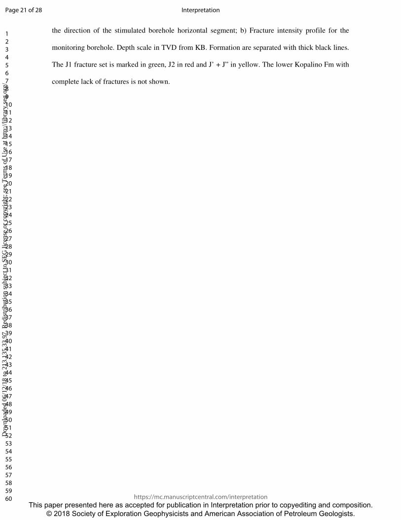
the direction of the stimulated borehole horizontal segment; b) Fracture intensity profile for the
monitoring borehole. Depth scale in TVD from KB. Formation are separated with thick black lines.
The J1 fracture set is marked in green, J2 in red and J’ + J” in yellow. The lower Kopalino Fm with
complete lack of fractures is not shown.
Page 21 of 28
https://mc.manuscriptcentral.com/interpretation
Interpretation
123456789101112131415161718192021222324252627282930313233343536373839404142434445464748495051525354555657585960
This paper presented here as accepted for publication in Interpretation prior to copyediting and composition. © 2018 Society of Exploration Geophysicists and American Association of Petroleum Geologists.
Dow
nloa
ded
06/1
2/18
to 2
13.1
35.3
3.97
. Red
istr
ibut
ion
subj
ect t
o SE
G li
cens
e or
cop
yrig
ht; s
ee T
erm
s of
Use
at h
ttp://
libra
ry.s
eg.o
rg/
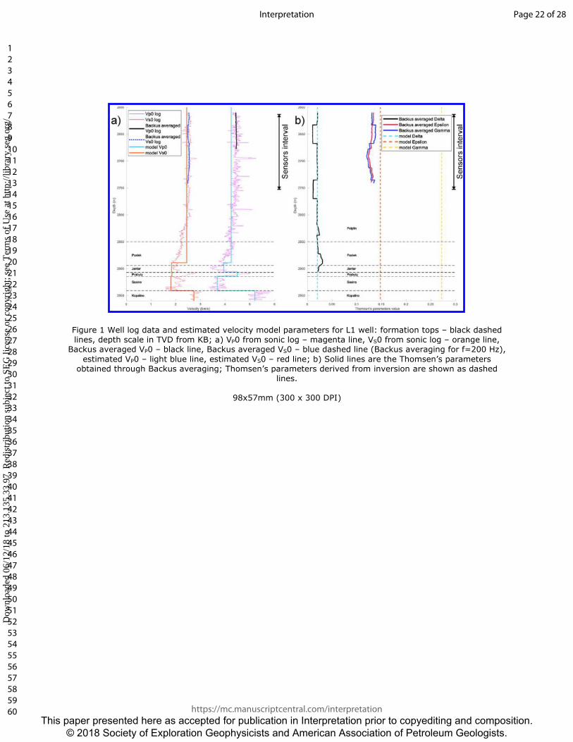
Figure 1 Well log data and estimated velocity model parameters for L1 well: formation tops – black dashed lines, depth scale in TVD from KB; a) VP0 from sonic log – magenta line, VS0 from sonic log – orange line,
Backus averaged VP0 – black line, Backus averaged VS0 – blue dashed line (Backus averaging for f=200 Hz),
estimated VP0 – light blue line, estimated VS0 – red line; b) Solid lines are the Thomsen’s parameters obtained through Backus averaging; Thomsen’s parameters derived from inversion are shown as dashed
lines.
98x57mm (300 x 300 DPI)
Page 22 of 28
https://mc.manuscriptcentral.com/interpretation
Interpretation
123456789101112131415161718192021222324252627282930313233343536373839404142434445464748495051525354555657585960
This paper presented here as accepted for publication in Interpretation prior to copyediting and composition. © 2018 Society of Exploration Geophysicists and American Association of Petroleum Geologists.
Dow
nloa
ded
06/1
2/18
to 2
13.1
35.3
3.97
. Red
istr
ibut
ion
subj
ect t
o SE
G li
cens
e or
cop
yrig
ht; s
ee T
erm
s of
Use
at h
ttp://
libra
ry.s
eg.o
rg/

Figure 2 Perforation shots locations in a vertical cross section aligned with borehole trajectory. True locations of all 16 perforations including 3 jet perforations are marked with yellow diamonds. 13 perforation shots locations in Backus averaged benchmark model are marked with stage-colored stars. Perforation shots
locations in the best obtained model are marked with stage-colored circles, depth scale in TVD from KB.
95x54mm (300 x 300 DPI)
Page 23 of 28
https://mc.manuscriptcentral.com/interpretation
Interpretation
123456789101112131415161718192021222324252627282930313233343536373839404142434445464748495051525354555657585960
This paper presented here as accepted for publication in Interpretation prior to copyediting and composition. © 2018 Society of Exploration Geophysicists and American Association of Petroleum Geologists.
Dow
nloa
ded
06/1
2/18
to 2
13.1
35.3
3.97
. Red
istr
ibut
ion
subj
ect t
o SE
G li
cens
e or
cop
yrig
ht; s
ee T
erm
s of
Use
at h
ttp://
libra
ry.s
eg.o
rg/
Figure 3 A map view of stage-colored perforations shots locations (a) and microseismic events locations scaled by moment magnitude spanning from -3.6 to -2.0 (b).
113x76mm (300 x 300 DPI)
Page 24 of 28
https://mc.manuscriptcentral.com/interpretation
Interpretation
123456789101112131415161718192021222324252627282930313233343536373839404142434445464748495051525354555657585960
This paper presented here as accepted for publication in Interpretation prior to copyediting and composition. © 2018 Society of Exploration Geophysicists and American Association of Petroleum Geologists.
Dow
nloa
ded
06/1
2/18
to 2
13.1
35.3
3.97
. Red
istr
ibut
ion
subj
ect t
o SE
G li
cens
e or
cop
yrig
ht; s
ee T
erm
s of
Use
at h
ttp://
libra
ry.s
eg.o
rg/

Figure 4 Comparison of mislocation and time residuals between initial Backus-averaged model (marked in orange) and final inverted (marked in blue) velocity models. In the mislocation section solid bars represent
horizontal component of location error, hatched bars represent vertical component of location error.
39x14mm (300 x 300 DPI)
Page 25 of 28
https://mc.manuscriptcentral.com/interpretation
Interpretation
123456789101112131415161718192021222324252627282930313233343536373839404142434445464748495051525354555657585960
This paper presented here as accepted for publication in Interpretation prior to copyediting and composition. © 2018 Society of Exploration Geophysicists and American Association of Petroleum Geologists.
Dow
nloa
ded
06/1
2/18
to 2
13.1
35.3
3.97
. Red
istr
ibut
ion
subj
ect t
o SE
G li
cens
e or
cop
yrig
ht; s
ee T
erm
s of
Use
at h
ttp://
libra
ry.s
eg.o
rg/

Figure 5 Comparison of the observed and modelled perforation shots moveouts.
94x52mm (300 x 300 DPI)
Page 26 of 28
https://mc.manuscriptcentral.com/interpretation
Interpretation
123456789101112131415161718192021222324252627282930313233343536373839404142434445464748495051525354555657585960
This paper presented here as accepted for publication in Interpretation prior to copyediting and composition. © 2018 Society of Exploration Geophysicists and American Association of Petroleum Geologists.
Dow
nloa
ded
06/1
2/18
to 2
13.1
35.3
3.97
. Red
istr
ibut
ion
subj
ect t
o SE
G li
cens
e or
cop
yrig
ht; s
ee T
erm
s of
Use
at h
ttp://
libra
ry.s
eg.o
rg/

Figure 6 Locations of stage-colored microseismic events scaled by moment magnitude spanning from -3.6 to -2.0 in vertical cross section aligned with the borehole trajectory, depth scale in TVD from KB.
95x53mm (300 x 300 DPI)
Page 27 of 28
https://mc.manuscriptcentral.com/interpretation
Interpretation
123456789101112131415161718192021222324252627282930313233343536373839404142434445464748495051525354555657585960
This paper presented here as accepted for publication in Interpretation prior to copyediting and composition. © 2018 Society of Exploration Geophysicists and American Association of Petroleum Geologists.
Dow
nloa
ded
06/1
2/18
to 2
13.1
35.3
3.97
. Red
istr
ibut
ion
subj
ect t
o SE
G li
cens
e or
cop
yrig
ht; s
ee T
erm
s of
Use
at h
ttp://
libra
ry.s
eg.o
rg/
Figure 7 a) Orientation of the sub-vertical fracture sets (joints) in the monitoring borehole and the present-day maximum horizontal stress direction (SHmax). The green dashed line points to the direction of the
stimulated borehole horizontal segment; b) Fracture intensity profile for the monitoring borehole. Depth
scale in TVD from KB. Formation are separated with thick black lines. The J1 fracture set is marked in green, J2 in red and J’ + J” in yellow. The lower Kopalino Fm with complete lack of fractures is not shown.
269x857mm (300 x 300 DPI)
Page 28 of 28
https://mc.manuscriptcentral.com/interpretation
Interpretation
123456789101112131415161718192021222324252627282930313233343536373839404142434445464748495051525354555657585960
This paper presented here as accepted for publication in Interpretation prior to copyediting and composition. © 2018 Society of Exploration Geophysicists and American Association of Petroleum Geologists.
Dow
nloa
ded
06/1
2/18
to 2
13.1
35.3
3.97
. Red
istr
ibut
ion
subj
ect t
o SE
G li
cens
e or
cop
yrig
ht; s
ee T
erm
s of
Use
at h
ttp://
libra
ry.s
eg.o
rg/
Top Related