


Languages
Pages
Legal

Wayne State UniversityDigital Commons@Wayne State University
Wayne State University Dissertations
1-1-2012
Reliability and effect of partially restrained woodshear wallsJohn Joseph GruberWayne State University, [email protected]
This Open Access Dissertation is brought to you for free and open access by Digital Commons@Wayne State University. It has been accepted forinclusion in Wayne State University Dissertations by an authorized administrator of Digital Commons@Wayne State University. For more information,please contact [email protected].
Recommended CitationGruber, John Joseph, "Reliability and effect of partially restrained wood shear walls" (2012). Wayne State University Dissertations. Paper442.http://digitalcommons.wayne.edu/oa_dissertations/442

RELIABILITY AND EFFECT OF PARTIALLY RESTRAINED WOOD SHEAR WALLS
by
JOHN J. GRUBER
DISSERTATION
Submitted to the Graduate School
of Wayne State University,
Detroit, Michigan
in partial fulfillment of the requirements
for the degree of
DOCTOR OF PHILOSOPHY
2012
MAJOR: CIVIL ENGINEERING
Approved by: _______________________________ Advisor Date
_______________________________
_______________________________
_______________________________
_______________________________

© COPYRIGHT BY
JOHN J. GRUBER
2012
All Rights Reserved

ii
DEDICATION
I dedicate this dissertation to my beloved wife, Jennifer.

iii
ACKNOWLEDGMENTS
I would like to thank Dr. Christopher Eamon, Dr. Wen Li and Dr. Hwai Chung Wu
for agreeing to serve on my dissertation committee.
I would like to thank my advisor, Dr. Gongkang Fu, for all the guidance, direction
and support he has given me throughout my Doctorate program and especially for
encouraging me to pursue this degree. I would also like to thank the faculty and staff of
the Department of Civil and Environmental Engineering at Wayne State University for all
the support and encouragement they have given me. A special thanks to the graduate
school for the Graduate Professional Scholarship I received for school years 2010/2011
and 2011/2012.
I would like to also thank others who have offered direction, advice, support, and
reviewing including Dr. Upul Attanayake, Dr. Dinesh Devaraj, Mr. Alexander Lamb,
Mrs. Renee Ryan, P.E., and my work partners Mr. Richard Hamann, P.E. and Mr. Craig
Anderson, P.E.
I would like to thank and recognize the Structural Building Components Research
Institute for the use of their test facility and support. This thesis would not have been
possible without their support. I would like to especially thank the lab technicians,
Mr. Keith Hershey and Mr. Michael Oftedahl, for their hard work and patience; Mr. Dan
Hawk for help with data management; and Mr. Kirk Grundahl, P.E., the executive
director of the Structural Building Components Association, for the initiative for this
project, encouragement, and support.

iv
Additional thanks and recognition go to Testing Engineers and Consultants and
Simpson Strong Tie. Testing Engineers and Consultants provided the lab for the
specific gravity tests. Simpson Strong Tie provided the mechanical hold down devices.
Finally, I would like to thank my family; my parents (posthumously), Jack and
Carol; my brother, Greg, and sisters, Sheila, Sharon, and Anne; my two sons, Jonathon
and Alexander, and my wife, Jennifer, for their encouragement, faith, support, and
patience throughout all of my studies. They have sacrificed a great deal for my
education and this research. I certainly could not have completed this without them.

v
TABLE OF CONTENTS
Dedication ....................................................................................................................... ii
Acknowledgements .........................................................................................................iii
List of Figures..................................................................................................................xi
List of Graphs................................................................................................................xiii
List of Tables..................................................................................................................xv
CHAPTER 1: INTRODUCTION...................................................................................... 1
1.1 History ........................................................................................................... 4
1.1.1 Historic House Data................................................................................... 4
1.1.2 Historic Wall Bracing.................................................................................. 6
1.1.3 Prescriptive Code History .......................................................................... 7
1.2 Reliability Analysis......................................................................................... 9
1.2.1 Testing....................................................................................................... 9
1.2.2 Verification of Empirical Partial Restraint Factor........................................ 9
1.2.3 Reliability Model......................................................................................... 9
1.3 Recommendations for Code Revisions ....................................................... 10
1.4 Organization of Thesis................................................................................. 11
CHAPTER 2: LITERATURE REVIEW.......................................................................... 13
2.2 2009 IRC Requirements .............................................................................. 13
2.2.1 Development of the 2009 IRC Requirements .......................................... 13
2.2.2 2009 IRC Requirements .......................................................................... 15
2.3 Differences between Prescriptive and Engineered Solutions ...................... 18
2.4 Actual Wind Load on a Shear Wall .............................................................. 20

vi
2.5 Partially and Unrestrained Shear Walls....................................................... 22
2.6 Special Design Provisions for Wind and Seismic (2005)............................. 27
2.7 Voluntary Product Standard ........................................................................ 30
2.8 APA Research Report 154 .......................................................................... 31
2.9 Shear Wall Strength and Computer Modeling ............................................. 33
2.9.1 Finite Element Modeling .......................................................................... 35
2.9.2 Sheathing Nail Modeling.......................................................................... 36
2.9.2.1 NDS Yield Limit Equations ................................................................... 37
2.9.2.1.1 Mode Im and Is ...................................................................................... 39
2.9.2.1.2 Mode II ................................................................................................. 39
2.9.2.1.3 Mode IIIm and IIIs .................................................................................. 39
2.9.2.1.4 Mode IV................................................................................................ 40
2.9.2.2 Load Deformation of Nails.................................................................... 40
2.10 Reliability Studies ........................................................................................ 42
2.11 IRC Brace wall Testing - SBC Research Institute........................................ 46
2.11.1 SBCRI Test Results................................................................................. 48
CHAPTER 3: TESTING OF SHEAR WALLS ............................................................... 51
3.1 Current ASTM Test Procedures .................................................................. 51
3.2 Wall Testing................................................................................................. 54
3.2.1 Test Facility.............................................................................................. 55
3.2.2 Wall Construction..................................................................................... 55
3.2.2.1 Wall Matrix ........................................................................................... 55
3.3 Test Results ................................................................................................ 56

vii
3.3.1 Data Results ............................................................................................ 56
3.3.2 Discussion of Wall Failures...................................................................... 62
3.3.3 Partial Restraint Effect ............................................................................. 64
3.3.4 Probability Distribution of Unit Shear Capacity ........................................ 66
3.3.5 Probability Distribution of Specific Gravity ............................................... 68
3.3.6 Wall Restrained with Hold Down.............................................................. 69
CHAPTER 4: FINITE ELEMENT MODELING.............................................................. 74
4.1 Finite Element Model................................................................................... 74
4.1.1 Elements.................................................................................................. 75
4.1.1.1 Framing Members ................................................................................ 76
4.1.1.2 Nails ..................................................................................................... 76
4.1.1.3 Sheathing Members ............................................................................. 77
4.1.2 Materials .................................................................................................. 77
4.2 Connections ................................................................................................ 79
4.3 Modeling...................................................................................................... 86
4.4 Finite Element Analysis Results .................................................................. 87
CHAPTER 5: RELIABILITY ANALYSIS ....................................................................... 97
5.1 Code Required Load Combinations ............................................................ 98
5.2 Reliability of SDPWS Nominal Unit Shear Capacities ................................. 98
5.2.1 Reliability Model..................................................................................... 101
5.2.2 Reliability Analysis Results .................................................................... 103
5.3 Base Calibration of Partially Restrained Unit Shear Capacities................. 104
5.4 Extended Calibration of Partially Restrained Unit Shear Capacities.......... 108

viii
5.4.1 Calibration with Reduced Dead Load Combinations.............................. 108
5.4.2 Calibration without a Variation in the Specific Gravity............................ 108
5.4.3 Random Variables used for Calibration ................................................. 109
5.4.4 Random Variable Distributions .............................................................. 112
5.4.5 Steps used for Monte Carlo Simulation.................................................. 112
5.4.6 Calculations for Monte Carlo Simulation................................................ 114
5.4.7 Results of the Monte Carlo Simulation for ASD ..................................... 119
5.4.8 Calibration with a Variation in the Specific Gravity................................. 122
5.4.9 Results of the Monte Carlo Simulation for ASD ..................................... 123
5.4.10 Results of the Monte Carlo Simulation for LRFD ................................... 125
5.4.11 Calibration with a Variation in the Specific Gravity................................. 128
5.4.12 Results of the Monte Carlo Simulation for LRFD ................................... 128
CHAPTER 6: DISCUSSION OF NOMINAL UNIT SHEAR VALUES.......................... 131
6.1 Difference in Method to Determine Unit Shear Values .............................. 131
6.1.1 SDPWS Values for Anchoring Device.................................................... 131
6.1.2 Use of ASTM E72 .................................................................................. 133
6.1.3 Use of ASTM E564 ................................................................................ 134
6.1.4 Partial Restraint Factors ........................................................................ 135
CHAPTER 7: SUMMARY, CONCLUSION, AND RECOMMENDATIONS FOR FUTURE
RESEARCH...................................................................................................... 137
7.1 Summary ................................................................................................... 137
7.2 Conclusions............................................................................................... 137
7.3 Recommendations for Future Research.................................................... 141

ix
Appendix A.................................................................................................................. 142
WALL TESTS .......................................................................................................... 142
A1 Wall Testing............................................................................................... 142
A2 Wall Materials............................................................................................ 142
A3 Wall Construction ...................................................................................... 145
A4 Test Setup................................................................................................. 150
A4.1 Test Fixture Setup.................................................................................. 150
A4.2 Test Frame ............................................................................................ 152
A5 Instrumentation.......................................................................................... 155
A5.1 Test Equipment Software....................................................................... 157
A5.2 Test Procedure ...................................................................................... 159
A5.2.1 Test Sequence....................................................................................... 159
A5.2.2 Test Loading .......................................................................................... 159
A5.2.3 Test Procedure ...................................................................................... 161
A5.2.4 Test Data ............................................................................................... 162
A6 Specific Gravity Test.................................................................................. 163
A6.1 Results of Specific Gravity Test ............................................................. 164
Appendix B.................................................................................................................. 170
SBCRI ACCREDITATION CERTIFICATE............................................................... 170
Appendix C.................................................................................................................. 172
STRING POTENTIOMETER AND LOAD CELL SPECIFICATIONS ....................... 172
Appendix D.................................................................................................................. 176
FOSM RELIABILITY OF SDPWS............................................................................ 176

x
Appendix E.................................................................................................................. 182
FOSM RELIABILITY OF WALL ............................................................................... 182
Appendix F .................................................................................................................. 188
MONTE CARLO SIMULATION................................................................................ 188
Appendix G ................................................................................................................. 189
EXAMPLE CALCULATIONS OF UNIT SHEAR....................................................... 189
References.................................................................................................................. 191
Abstract ....................................................................................................................... 197
Autobiographical Statement ........................................................................................ 199
xi
LIST OF FIGURES
Figure 1: Continental US Shaded Wind Speed Map (WBDG 2010)............................... 2
Figure 2: IRC Braced Wall Panel Location (IRC) ......................................................... 16
Figure 3: IRC Braced Wall Panel Length...................................................................... 17
Figure 4: Engineered Shear Wall Restraint Methods ................................................... 19
Figure 5: Hysteresis Curve Example ............................................................................ 33
Figure 6: Hysteretic Response of a Sheathing-to-Framing Connector ......................... 34
Figure 8: Connection Yield Modes ............................................................................... 38
Figure 9: SBC Research Institute Test Building (SBCRI) ............................................. 47
Figure 10: SBCA Research Institute Wall Failure (SBCARI T-IRC).............................. 47
Figure 11: Standard Wood Frame (ASTM E72) ........................................................... 52
Figure 12: Test Assembly Wall A ................................................................................. 71
Figure 13: Test Assembly Walls B, C and D ................................................................ 72
Figure 14: Test Assembly Wall E ................................................................................. 73
Figure 15: Finite Element Model................................................................................... 75
Figure 17: FEM of Stud Connection ............................................................................. 83
Figure 18: FEM Results of Stud Connection Rigidity.................................................... 84
Figure 19: Sole Plate Deformation of Wall E................................................................ 93
Figure 20: Deformation of Wall A FE Model ................................................................. 95
Figure 22: ASTM E72 Test Fixture............................................................................. 132
Figure 23: Test Setup................................................................................................. 151
Figure 24: Load Cell ................................................................................................... 156
Figure 25: String Potentiometer ................................................................................. 156

xii
Figure 26: Data Acquisition Software Graphics Display ............................................. 158
Figure 27: Actuator Control Software Load Steps ...................................................... 159

xiii
LIST OF GRAPHS
Graph 1: Effect of Uplift Restraint on the Lateral Load Capacity of a Shear Wall Based on Mechanics-Based Approach (Ni and Karacabeyli 2000) .......................... 24
Graph 2: Effect of Uplift Restraint on the Lateral Load Capacity of a Shear Wall Based on Empirical Approach (Ni and Karacabeyli 2000) ........................................ 25
Graph 3: Nail Deformation Model................................................................................. 42
Graph 4: Probability Density Function of Shear Wall Load........................................... 44
Graph 5: Failure Region of PDF of Shear Wall Load.................................................... 45
Graph 6: Reliability Index, β, on the Standard Normal Distribution............................... 46
Graph 7: Hysteresis Curve for Wall A1......................................................................... 57
Graph 8: Summary of Wall Tests ................................................................................. 58
Graph 9: 8d Common Nail Curves from Wall Group A.................................................. 59
Graph 10: 8d Common Nail Curve Model .................................................................... 60
Graph 11: Hold down Stiffness from Test Results........................................................ 62
Graph 12: Partial Restraint Effect on Strength ............................................................. 65
Graph 13: Unit Shear Capacity of Wall A on Normal Probability Paper........................ 66
Graph 14: Unit Shear Capacity of Wall A on Log-Normal Probability Paper ................ 67
Graph 15: Correlation of Wall Strength to Specific Gravity........................................... 70
Graph 16: Sheathing Nail Data for ABAQUS ............................................................... 80
Graph 17: 16d Stud Withdrawal Nail Data for ABAQUS............................................... 82
Graph 18: Effect of Axial Load on Stud Connection Rigidity ........................................ 84
Graph 19: Hold Down Stiffness for ABAQUS ............................................................... 86
Graph 20: FE Comparison for Wall A........................................................................... 88
Graph 21: FE Comparison for Wall B........................................................................... 88

xiv
Graph 22: FE Comparison for Wall C........................................................................... 89
Graph 23: FE Comparison for Wall D........................................................................... 89
Graph 24: FE Comparison for Wall E........................................................................... 90
Graph 25: FE Model of Fully Restrained wall Compared to FE Model of Walls A-E .... 90
Graph 26: Comparison of FE Model to Test Results.................................................... 92
Graph 27: Contour Plot of Corner Nail Vertical Force, Wall E...................................... 94
Graph 28: Calibration of Unrestrained Shear Wall ..................................................... 106
Graph 29: Partial Restraint Effect on Strength - Calibrated......................................... 107
Graph 30: Comparison of Calibrated Partial Restraint Effect ..................................... 108
Graph 31: Partial Restraint Effect, ASD, without Specific Gravity .............................. 121
Graph 32: Partial Restraint Effect, ASD, with Specific Gravity ................................... 125
Graph 33: Partial Restraint Effect, LRFD, without Specific Gravity ............................ 127
Graph 34: Partial Restraint Effect, LRFD, with Specific Gravity ................................. 130
Graph 35: Comparison of Partial Restraint................................................................. 136
Graph 36: Wall Group A Loading ............................................................................... 160
Graph 37: Distribution of the Specific Gravity for SPF-S Studs.................................. 165
Graph 38: Distribution of the Specific Gravity for OSB Sheathing.............................. 166
xv
LIST OF TABLES
Table 1: Historic House Data (HUD 2001) ..................................................................... 5
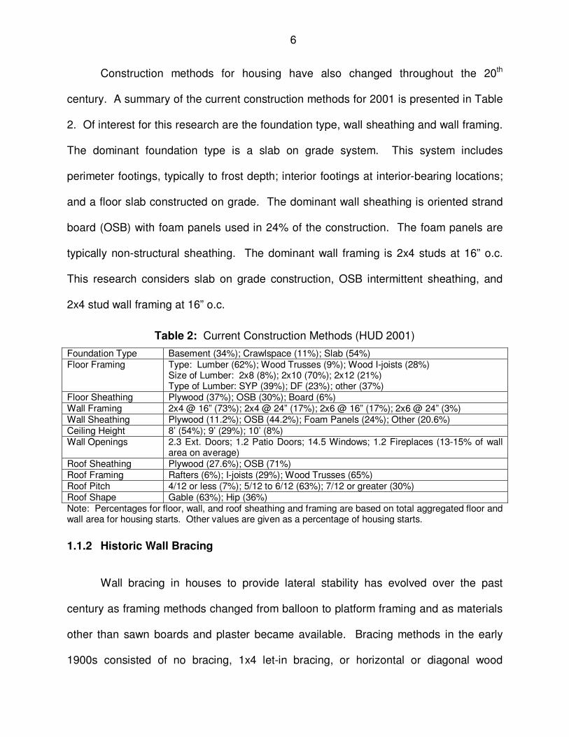
Table 2: Current Construction Methods (HUD 2001)...................................................... 6
Table 3: Interior Wall Amounts (HUD 2001) ................................................................... 8
Table 4: Nominal Shear Strength Adjustment Factors for Conventional Wall Bracing .. 15
Table 5: Summary of Test Data (Seaders 2004).......................................................... 26
Table 6: Nominal Unit Shear Capacities for Wood-Frame Shear Walls (SDPWS 2005)...................................................................................... 28
Table 7: APA Test Comparisons (APA 2004)............................................................... 32
Table 8: Summary of SBCRI Tests ............................................................................... 48
Table 9: Comparison of SBCRI, Seaders, SDPWS...................................................... 49
Table 10: Comparison of Seaders to SDPWS.............................................................. 49
Table 11: Test Matrix.................................................................................................... 56
Table 12: Summary of Wall Ultimate Unit Shear Capacity ........................................... 58
Table 13: Nail Values from Wall Group A..................................................................... 61
Table 14: Wall Group A Normal Distribution Probability ............................................... 66
Table 15: Summary of Specific Gravity Tests .............................................................. 68
Table 16: Effectiveness of Hold Down.......................................................................... 70
Table 17: Framing Material .......................................................................................... 78
Table 18: Sheathing Material ....................................................................................... 79
Table 19: Sheathing Nail Data ..................................................................................... 80
Table 20: Stud to Plate Vertical Nail Data .................................................................... 81
Table 21: Hold Down Stiffness Data............................................................................. 85
xvi
Table 22: Summary of FE Model Constraints............................................................... 87
Table 23: Comparison of FE Model to Test Results..................................................... 91
Table 24: Load Combinations ...................................................................................... 98
Table 25: Excerpt from APA Report 154, Table A1...................................................... 99
Table 26: Excerpt from APA Report 154, Table A2...................................................... 99
Table 27: Summary of APA Report 154 ..................................................................... 100
Table 28: Comparison of SDPWS Nominal Unit Shear to the 5th Percentile .............. 101
Table 29: Summary of Distributions ............................................................................ 102
Table 30: Nominal Unit Shear Calibration for Unrestrained Wall E ............................ 105
Table 31: Calibrated Shear Wall Capacities............................................................... 107
Table 32: Summary of Distributions ............................................................................ 112
Table 33: Summary of MCS for ASD without Specific Gravity ................................... 120
Table 34: Summary of Distributions ............................................................................ 122
Table 35: Summary of MCS for ASD with Specific Gravity ........................................ 124
Table 36: Summary of MCS for LRFD without Specific Gravity ................................. 126
Table 37: Summary of MCS for LRFD with Specific Gravity ...................................... 129
Table 38: Design Restraining Force for IRC Shear Wall ............................................ 140
Table 39: Lumber Materials........................................................................................ 142
Table 40: OSB Measurements ................................................................................... 145
Table 41: Test Equipment ........................................................................................... 156
Table 42: Chi-Square Test for Specific Gravity Probability Distribution for Studs ...... 165
Table 43: Specific Gravity of Members in Wall Group A............................................. 167
Table 44: Specific Gravity of Members in Wall Group B............................................. 167

xvii
Table 45: Specific Gravity of Members in Wall Group C ............................................ 168
Table 46: Specific Gravity of Members in Wall Group D ............................................ 168
Table 47: Specific Gravity of Members in Wall Group E............................................. 169

1
CHAPTER 1
INTRODUCTION
The purpose of this research is to examine the reliability levels of the prescriptive
wall bracing requirements of the 2009 International Residential Code (IRC) and the
engineered shear wall requirements of the 2009 International Building Code (IBC) along
with the 2005 Special Design Provisions for Wind and Seismic (AF&PA SDPWS). This
research encompasses structures constructed in 90 m.p.h. wind areas with exposure B.
In order to understand the focus of the proposed research, it is necessary to
understand the history of housing, housing construction practices, and wall bracing.
Based upon the ASCE 7 wind speed map shown in Figure 1, this research affects the
majority of the housing in the continental United States since it applies to structures in
low wind speed and low seismic areas. Currently, a prescriptive design method is
dominant for the design of lateral bracing for single family houses. When the limits of
the prescriptive design are exceeded, then an engineered alternative is necessary.
Based on the information available today, the reliability levels of these two design
methods are not equivalent. It is desirable to understand the reliability levels of these
two systems and compare them.
The reliability analysis is useful for several reasons. First, it provides a
comparison of the two design philosophies in a way that is independent of the design
methods by using the second-moment reliability index β. This “provides a relative
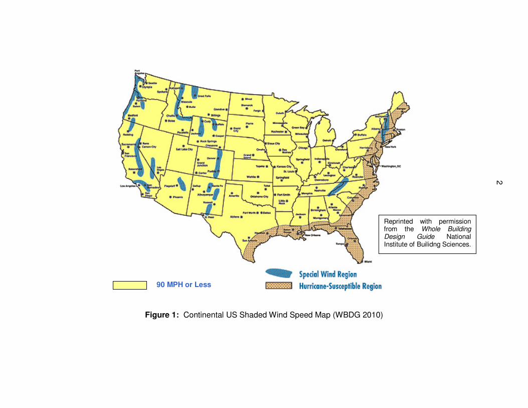
Figure 1: Continental US Shaded Wind Speed Map (WBDG 2010)
90 MPH or Less
Reprinted with permission from the Whole Building Design Guide National Institute of Builidng Sciences.
2

3
measure of the safety of a structural component or system and serves as the
cornerstone of code calibration studies” (van de Lindt and Rosowsky 2005). Second,
the study is useful to calibrate resistance factors to unify the two design methods with
respect to structural safety. This is beneficial for alternate building materials and
systems that could provide economic, energy or sustainability benefits.
This research provides the following items:
1. The reliability index of the unit shear capacity for 15/32” Wood Structural
Panels (WSP) in SDPWS (2005)
2. The appropriateness of ASTM E72 for walls anchored with mechanical
hold downs and partially restrained IRC (2009) prescriptive walls.
3. Verification for the resistance factor used by the SDPWS.
4. Recommended codified nominal unit shear design values for wind load
for unrestrained shear walls constructed in accordance with the 2009
IRC using 15/32” WSP.
5. Recommended codified nominal unit shear design values for wind load
for fully restrained shear walls constructed in accordance with the 2009
IRC using 15/32” WSP.
6. Proposed requirement for unrestrained shear wall tests for WSP
manufacturers in the Voluntary Product Standard PS 2-04 titled
Performance Standards for Wood-Based Structural-Use Panels (NIST
2004) for WSP.

4
7. Recommended IRC utilization of the unrestrained shear wall nominal
unit shear design values or definition of some minimum restraining
force to be known present.
The above results will create an equitable design methodology between the IRC
prescriptive method and the SDPWS. When implemented and utilized in the IRC,
alternate products and engineered alternatives can be provided without the appearance
of over-conservatism.
1.1 History
1.1.1 Historic House Data
The total load resistance of wall bracing in houses is not only dependent upon
the material, but also the spacing of brace wall lines and aspect ratios of brace walls.
The spacing of the brace wall lines obviously affects the tributary wind area of each
brace wall line. The aspect ratios typically affect the strength and certainly affect the
stiffness of the brace walls. Therefore, the number of openings in a wall as well as the
height of a wall can affect the load resistance of the lateral load resisting system. These
geometric features have been changing during the past century, creating a greater
demand on lateral bracing systems.
Beyond the structural history of brace walls, the economic value of homes is also
of concern. As the value of homes increase, the financial risk due to wind damage also
increases.

5
Table 1 shows a comparison of house construction over the 20th century. The
average size of houses more than doubled in this period of time, while the number of
bedrooms remained about the same. Today’s homes include more large open spaces
than homes built in the early 1900s. Over the same time period, housing costs have
increased by a factor of 100. The inflation-adjusted housing cost in the early 1900s was
about $35.00/sq. ft. The cost in 2000 was about $100.00/sq. ft.
Table 1: Historic House Data (HUD 2001)
Early 1900’s Mid 1900’s Late 1900’s
Population 76 Million (40% urban, 60% rural)
150 Million (64 % urban, 36% rural)
270 Million (76% urban, 24% rural)
Median Family Income $490 $3,319 $45,000 New Home Price Average Unknown
1 $11,000 $200,000
Type of Purchase Typically Cash FHA Mortgage, 4.25% (few options)
8% (many options)
Ownership Rate 46 % 55% 67% Total Housing Units 16 Million 43 Million 107 Million (approx. 50%
single-family) Number of annual housing starts
189,000 (65% single-family)
1.95 Million (85% single-family)
1.54 Million (approx. 50% single family)
Average Size (starts) < 1,000 sq. ft. 1,000 sq. ft. 2,000 sq. ft. or more Stories 1 to 2 1 (86%); 2 or more
(14%) 1 (48%); 1½ or 2 (49%)
Bedrooms 2 to 3 2 (66%); 3 (33%) 2 or less (12%); 3 (54%); 4 or more (34%)
Bathrooms 0 or 1 1½ or less (96%) 1½ or less (7%); 2 (40%); 2½ + (53%)
Garage 1 car (41%); 0 (53%) 2 car (65%)
Table 1 also indicates that there has been a large movement to urban settings
from rural. The shift from rural to urban settings indicates that wind exposure is
decreasing as the exposure category is B for urban locations and typically C for rural
locations (ASCE 7-05).
1 Based on “Housing at the Millennium: Facts, Figures, and Trends,” the average new home cost was less
than $5,000. However, this estimate is potentially skewed in that many people could not afford a “house” of the nature considered in the study. Based on Sears, Roebuck, and Co. catalogue prices at the turn of the century, a typical house may have ranged from $1,000 to $2,000, including land.
6
Construction methods for housing have also changed throughout the 20th
century. A summary of the current construction methods for 2001 is presented in Table
2. Of interest for this research are the foundation type, wall sheathing and wall framing.
The dominant foundation type is a slab on grade system. This system includes
perimeter footings, typically to frost depth; interior footings at interior-bearing locations;
and a floor slab constructed on grade. The dominant wall sheathing is oriented strand
board (OSB) with foam panels used in 24% of the construction. The foam panels are
typically non-structural sheathing. The dominant wall framing is 2x4 studs at 16” o.c.
This research considers slab on grade construction, OSB intermittent sheathing, and
2x4 stud wall framing at 16” o.c.
Table 2: Current Construction Methods (HUD 2001)
Foundation Type Basement (34%); Crawlspace (11%); Slab (54%) Floor Framing Type: Lumber (62%); Wood Trusses (9%); Wood I-joists (28%)
Size of Lumber: 2x8 (8%); 2x10 (70%); 2x12 (21%) Type of Lumber: SYP (39%); DF (23%); other (37%)
Floor Sheathing Plywood (37%); OSB (30%); Board (6%) Wall Framing 2x4 @ 16” (73%); 2x4 @ 24” (17%); 2x6 @ 16” (17%); 2x6 @ 24” (3%) Wall Sheathing Plywood (11.2%); OSB (44.2%); Foam Panels (24%); Other (20.6%) Ceiling Height 8’ (54%); 9’ (29%); 10’ (8%) Wall Openings 2.3 Ext. Doors; 1.2 Patio Doors; 14.5 Windows; 1.2 Fireplaces (13-15% of wall
area on average) Roof Sheathing Plywood (27.6%); OSB (71%) Roof Framing Rafters (6%); I-joists (29%); Wood Trusses (65%) Roof Pitch 4/12 or less (7%); 5/12 to 6/12 (63%); 7/12 or greater (30%) Roof Shape Gable (63%); Hip (36%) Note: Percentages for floor, wall, and roof sheathing and framing are based on total aggregated floor and wall area for housing starts. Other values are given as a percentage of housing starts.
1.1.2 Historic Wall Bracing
Wall bracing in houses to provide lateral stability has evolved over the past
century as framing methods changed from balloon to platform framing and as materials
other than sawn boards and plaster became available. Bracing methods in the early
1900s consisted of no bracing, 1x4 let-in bracing, or horizontal or diagonal wood

7
sheathing (HUD 2001). The method of no bracing apparently relied on the interior wood
lath and plaster for the bracing system.
As early as 1929 the Forest Products Laboratory began comparison testing of
various bracing methods (HUD 2001). The walls tested were 9’ x 14’ and
7’-4” x 12’ with enough vertical restraint to prevent over-turning. These walls were
either solid, had one window opening, or had one window and one door opening. The
results of the tests are presented in (HUD 2001).
1.1.3 Prescriptive Code History
Plywood was introduced in the mid 1900s. This renewed the interest in bracing
methods. Plywood is typically manufactured in 4’ x 8’ sheets and is installed either
continuously over the exterior walls or intermittently. Until the early 2000s, with the
introduction of the International Codes (a combination of the BOCA, UBC, and SBC),
the primary bracing methods in the late 1900s were metal T-bracing, wood structural
panels (plywood or OSB), or gypsum.
Table 1 shows that houses are larger, but don’t have more rooms, therefore
houses have larger rooms today than they did a century ago. This, coupled with larger
window and door openings, has led to less lateral resistance in houses. Although
typically discounted, interior partitions provide additional strength and stiffness to the
lateral resisting system of houses. The percentage of interior partitions in comparison
to floor area has decreased with the increased house size and especially with the large
open spaces enjoyed in the later part of the 1900s. Table 3 summarizes the change in
the amount of interior walls from early last century to late last century. Note that there is

8
a 1.1% and 1.7% reduction in interior walls, as a percent of floor area, for the second
and first floor of two-story houses respectively.
Table 3: Interior Wall Amounts (HUD 2001) (Lineal feet as a percent of floor area of story)
OLDER HOMES (early 1900s)1 MODERN HOMES (late 1900s)2
1 Story 9% ± 1% 1st Floor of 1 to 2 Story 4.3% ± 1% 1st Floor of 2 Story 6% ± 1% 2nd Floor of 2 Story 7.9% ± 1%
2nd Floor of 2 Story 9% ± 1.5% Notes: 1Values based on a small sample of traditional house plans in Sears Catalogues (1910-1926) including
affordable and more expensive construction of 1 and 2 stories. 2Values based on a small sample of representative modern home plans (1990s) including economy
and move-up construction (no luxury homes).
By the late 1900s, Hurricane Andrew and the Northridge Earthquake had
highlighted the importance of lateral bracing in houses. This timing, along with the
development of the International Codes, changed the bracing methods used in
prescriptive design. Much research of wood shear walls and bracing methods focused
on seismic design and cyclic testing. As a result, the codes began prescribing more
lateral bracing.
The current IRC (IRC 2009) uses more of a rational design method to prescribe
wall bracing to resist wind loads than previous editions but varies greatly from the
typical rational (engineered) design method using the ASCE 7-05 and the SDPWS. The
current IRC (IRC 2009) has also made an attempt to utilize both partial wall restraint
and a whole house effect. It is the goal of this research to compare the reliability of the
prescriptive design with the rational design using SDPWS.

9
1.2 Reliability Analysis
1.2.1 Testing
As part of this research, (25) 4’ x 8’ brace walls were monotonically load tested.
These walls varied from full restraint (a mechanical hold down device) to unrestrained
(only a single anchor bolt). The testing was performed at the Structural Building
Components Research Institute located in Madison, WI. The goal of the testing was to
understand the load-deflection behavior and ultimate strength of the varying restraint
conditions and the variability of the ultimate strength.
1.2.2 Verification of Empirical Partial Restraint Factor
The test data was used to verify the empirical partial restraint factor previously
developed by Ni and Karacabeyli (2000). This factor is intended to predict the capacity
of an unrestrained or partially restrained shear wall using the nominal unit shear
strength of a fully restrained wall. Differences between the IRC prescriptive sole plate
anchorage and the anchorage used to develop the empirical partial restraint factor
necessitate a verification of this factor for the IRC wall.
1.2.3 Reliability Model
Using the test results from the 25 tests, ultimate strengths and variability were
used in a first order second moment reliability model (FOSM) and Monte Carlo
Simulation (MCS) to determine the reliability index, β, for the current SDPWS nominal
unit shear strength and the nominal unit shear strength used in the 2009 IRC. The tests
results were also used to identify the random variables used in the reliability model.

10
The reliability analysis used both numerical analysis and Monte Carlo simulation to
evaluate the model.
Once the model was constructed for the varying wall restraint conditions, two
items were varied to provide a target value for β (3.25) for each of these conditions
which is similar to the current reliability index of 3.27 for the SDPWS nominal values.
These items included the resistance factor, φ, and the nominal tabulated unit shear
values for the varying cases.
1.3 Recommendations for Code Revisions
The conclusions of this research include recommendations for code revisions for
unrestrained, partially restrained, and fully restrained shear walls constructed with WSP
with 8d common nails and recommendations for finite element models. These are
based on a 4’x8’ WSP shear wall. The following is a list of these conclusions.
1. The reliability index of the SDPWS nominal unit shear value for 15/32” WSP
was determined using the allowable stress design (ASD) reduction factor and
resistance factor, φ, and APA Research Report 154 (APA 2004).
2. The use of ASTM E72 is inappropriate to determine nominal unit shear design
values.
3. Present nominal unit shear values published in SDPWS cannot be achieved
with a mechanical hold down at the base of the wall.
4. Using reliability analysis for calibration, partial restraint modification factors
are determined for both mechanical hold downs and a dead load restraining
force. These modification factors will be used to modify the nominal unit

11
shear capacity values in SDPWS. These modification factors are presented
for both allowable stress design (ASD) and load and resistance factored
design (LRFD) methods.
5. For equitable designs providing the same level of safety, the IRC 2009 should
publish the required dead load restraining force to achieve the unit shear
design value used. This restraining force should be clearly stated as a design
requirement for the use of the prescriptive method.
6. Finite element models should always include the effect of the boundary
conditions, restraining force, and the connection behavior of the studs-to-
top/sole-plate connections.
1.4 Organization of Thesis
Chapter 2 provides a literature review of codes and standards applicable to this
thesis; previous research regarding partially restrained wood shear walls; finite element
modeling; and reliability studies. The background of the prescriptive wall bracing
methods, design philosophy, and engineered alternate design methods are reviewed to
provide the reader with a basis for this thesis. Finite element modeling methods, nail
strength and load deformation modeling, as well as the nail yield limit theory are
reviewed. A reliability analysis of wood shear walls with wind loads conducted by van
de Lindt is also presented.
In Chapter 3 a summary of the wood shear wall testing conducted is presented.
This includes a brief overview of both ASTM E72 and E564. Summary of data obtained
from the test program that is used for both the finite element modeling and the reliability
study is presented here.

12
In Chapter 4 a finite element model is presented. This model includes a non-
linear finite element model created to simulate the behavior of partially restrained wood
shear walls and shear walls restrained with a mechanical hold down. This model
utilizes nonlinear orthogonal spring pairs using data obtained from the tests conducted.
Results from the finite element model are presented at the end of CHAPTER 4.
In Chapter 5, a systematic reliability analysis is presented. This analysis
concludes with a Monte Carlo simulation including four random variables: wind load,
dead load, wall unit shear capacity, and specific gravity. A partial restraint factor was
developed by calibrating the bias factor with the M-C simulation so that a constant
reliability index of 3.25 is obtained for all restraint conditions for the 4’x 8’ wood shear
wall.
A discussion regarding the intent and use of both ASTM E72 and E564 is
presented in Chapter 6. This describes the limitations of ASTM E72 and the
appropriateness of its use for determining design values.
Conclusions of this thesis are presented in Chapter 7. A brief summary of this
thesis is included here as well as suggestions for future research. The calibrated partial
restraint factors for both allowable stress design (ASD) and load and resistance factored
design (LRFD) are summarized.

13
CHAPTER 2
LITERATURE REVIEW
In this chapter a general introduction is given to the current design requirements
for intermittent brace walls in residential construction, a review of previous reliability
studies, a review of previous finite element modeling methods, and a review of recent
IRC wall testing. Specifically, the prescriptive requirements of the 2009 International
Residential Code (IRC) is discussed as well as requirements for an alternate
engineered design utilizing the 2009 International Building Code (IBC); Minimum Design
Loads for Buildings and Other Structures (ASCE 7-05); and the 2005 Special Design
Provisions for and Seismic (SDPWS) (AF&PA SDPWS).
2.2 2009 IRC Requirements
2.2.1 Development of the 2009 IRC Requirements
The 2009 IRC is the result of years of empirical methods. “The art and science
behind accurately understanding conventional wall bracing is still considered to be in its
infancy and subject to disparate interpretations, even though it has been studied at
various times since the early 1900s and especially in recent years,” (Crandell 2007).
The development of the 2009 IRC wind load provisions occurred under the
direction of an Ad Hoc Committee-Wall Bracing (AHC-WB). The AHC-WB was created
by the International Code Council (ICC). The AHC-WB committee had the support of a
second group led by Dan Dolan, PhD, which was supported by The Building Seismic
Safety Council (BSSC) (Crandell and Martin 2009).
14
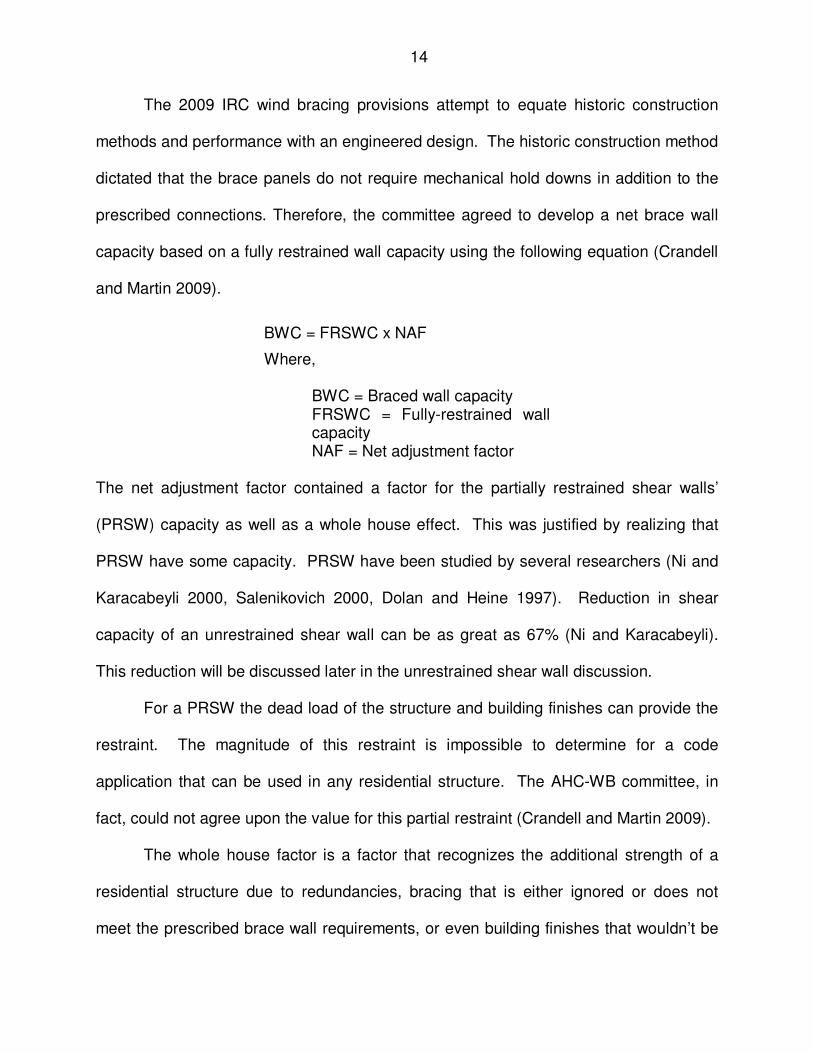
The 2009 IRC wind bracing provisions attempt to equate historic construction
methods and performance with an engineered design. The historic construction method
dictated that the brace panels do not require mechanical hold downs in addition to the
prescribed connections. Therefore, the committee agreed to develop a net brace wall
capacity based on a fully restrained wall capacity using the following equation (Crandell
and Martin 2009).
BWC = FRSWC x NAF
Where,
BWC = Braced wall capacity FRSWC = Fully-restrained wall capacity NAF = Net adjustment factor
The net adjustment factor contained a factor for the partially restrained shear walls’
(PRSW) capacity as well as a whole house effect. This was justified by realizing that
PRSW have some capacity. PRSW have been studied by several researchers (Ni and
Karacabeyli 2000, Salenikovich 2000, Dolan and Heine 1997). Reduction in shear
capacity of an unrestrained shear wall can be as great as 67% (Ni and Karacabeyli).
This reduction will be discussed later in the unrestrained shear wall discussion.
For a PRSW the dead load of the structure and building finishes can provide the
restraint. The magnitude of this restraint is impossible to determine for a code
application that can be used in any residential structure. The AHC-WB committee, in
fact, could not agree upon the value for this partial restraint (Crandell and Martin 2009).
The whole house factor is a factor that recognizes the additional strength of a
residential structure due to redundancies, bracing that is either ignored or does not
meet the prescribed brace wall requirements, or even building finishes that wouldn’t be

15
considered in an engineering analysis. Some may refer to this as a “system effect”
factor. According to Crandell and Martin 2009, five whole house tests were reviewed to
determine the value of this factor when compared to the IRC bracing method. Three of
these tests are described (Crandell and Martin 2009). They are the BRANZ, CSIRO,
and CUREe/FEMA. The ratio of tested values (failure) to the predicted (ultimate) values
ranged from 1.5 (discounting interior partitions) to 3.1. The Dolan-AHC-WB committee
could not reach a consensus on either of the two factors, but did agree to one factor,
1.2, which includes both factors (Crandell and Martin 2009). Crandell reported the
factors discussed by the committee and they are shown here in Table 4.
Table 4: Nominal Shear Strength Adjustment Factors for Conventional Wall Bracing
Walls Supporting: Partial-Restraint Factor
Whole Building Factor
Net Adjustment Factor
Roof Only 0.8 1.5 1.2 Roof + One Story 0.9 1.33 1.2
Roof + Two Stories 1.0 1.2 1.2 1. These factors are limited to residential construction in accordance with the 2009 IRC and
bracing methods that have a nominal shear strength “capped” at about 700 plf.
Therefore, a PRSW has a 20% advantage to a fully restrained shear wall that
does not include the whole building factor. The committee placed a further limit on the
brace wall requirements. This limit is that the net uplift at the top of the brace wall shall
not exceed 100 plf. If this is exceeded, then an additional connection at the base of the
wall is required.
2.2.2 2009 IRC Requirements
The IRC has several options for providing lateral bracing to a residential
structure. The lateral forces on the structure are resisted by braced wall panels. The

16
braced wall panels can be constructed with either continuous sheathing methods or
intermittent bracing methods. Intermittent braced wall panels can include diagonal let-in
bracing, diagonal sheathing, horizontal siding, or portals. The option which is the focus
of this thesis is intermittent braced wall panel construction, as shown in Figure 2,
utilizing the Wood Structural Panel (WSP) bracing option. The WSP option can be
thought of as a shear wall but is constructed differently than traditional engineered wood
shear walls, i.e. they may not have a special hold down connector.
Figure 2: IRC Braced Wall Panel Location (IRC)
The IRC provides a prescriptive method of lateral bracing for residential
structures. The bracing requirements are dependent upon both wind loads and seismic
loads. For each lateral load condition, the IRC tabulates the total length of braced wall
panels per braced wall line as well as braced wall line spacing. A braced wall line is a
wall selected by the designer to contain braced wall panels. The designer then selects
the braced wall panel type. The braced wall panels must then be located within the
Figure 602.10.1.4(2) Excerpted from the 2009 International Residential Code, Copyright 2009. Washington, D.C.: International Code Council. Reproduced with permission. All rights reserved. www.ICCSAFE.org

17
braced wall lines as specified in the IRC. For WSP, the minimum panel width for the
intermittent brace panel method is 48” and the minimum panel thickness is 3/8”. This
thesis will be limited to wind loading and not seismic loading.
Figure 3: IRC Braced Wall Panel Length
The IRC tabulates the braced wall panels by basic wind speed varying from
85 m.p.h. to 110 m.p.h. A series of adjustment factors are then applied to the tabulated
length of brace wall panels. These factors include: exposure and building height
adjustment; roof to eave height adjustment; number of braced wall line adjustment (to
account for increased shear on braced wall lines from continuous diaphragms, see
discussion below); and an adjustment factor if gypsum or equivalent is not installed on
the interior face of the wall panel. An example of a required length of a braced wall line
is given in Figure 3.
The IRC also specifies all of the connections required for the braced wall panels
as well as the connections of the structure to the wall panels. This includes the
sheathing fastening to the studs, the studs to the plates, the sole plate to the floor or
8'Say L ←=××××= '94.74.19.07.00.19'
Wind Speed = 90 mph → 9’ Braced Panel Length Required Exposure B, 1 Story, 8 ft walls → Multiply x1 Roof Eave-to-Ridge Height <6’ → Multiply by 0.7 and 0.9 No gypsum on interior → Multiply by 1.4 Required Braced Panel Length including all factors:
From IRC Section R602.10.1.2 and Table R602.10.1.2(1)

18
foundation, and the roof or floor to the wall top plate. The sheathing fastening is typical
for a braced wall panel and ordinary sheathing.
The IRC bracing method distributes the lateral loads equally amongst brace wall
panels. This is because it is assumed that the braced wall lines have the minimum
lengths of brace wall panels and therefore are of equal stiffness. Whole building tests
have shown that roof systems behave more like rigid diaphragms than flexible
diaphragms (Crandell and Kochkin 2003). Therefore, the IRC includes an adjustment
factor to increase the length of the braced wall when two or more brace wall lines exist.
This factor is 1.3 for 3 braced wall lines, 1.45 for 4 braced wall lines, and 1.6 for 5 or
more braced wall lines.
Aside from the combined partial restraint and whole building factor of 1.2
discussed earlier, the IRC uses a rational approach. For WSP, the nominal brace wall
capacity used is 700 plf which includes 200 plf capacity for ½” gypsum applied to the
interior face (Crandell and Martin 2009). Using allowable stress design (ASD), a factor
of safety of 2 was applied to the nominal value. This is in accordance with the 2005
Special Design Provisions for and Seismic (AF&PA SDPWS).
2.3 Differences between Prescriptive and Engineered Solutions
The major difference between the prescriptive design of the 2009 IRC and a
rational design using SDPWS is that the IRC applies a combined partial restraint and
whole building factor of 1.2 discussed earlier. An engineered design typically neglects
any applied dead load to the wall and requires a special hold down connector. This is
illustrated in Figure 4.

19
Figure 4: Engineered Shear Wall Restraint Methods
In order to resist the uplift force in a WSP shear wall, one of three methods must
be present for equilibrium. These are a special hold down connector, a dead load force
applied at the tension chord, or some other dead load applied along the wall. It is
common engineering practice to provide a special hold down connector neglecting any
dead loads. This assures that there is a proper load path to resist the overturning of
the wall. If a dead load occurs directly over the tension chord, this could be used to
restrain or partially restrain the wall, but it has a major limitation for an engineered
approach. This limitation is the load combination that requires using only 60% of the
dead load to resist wind overturning forces (ASCE 7). This 40% reduction can have a
huge impact on the uplift resistance. For the last option, special fastening of the wall
sheathing is required. From a mechanics analysis of the wall, the sheathing resists the
V
T C
V
V
P
C
V
HOLD DOWNCONNECTOR
a) Restrained With Hold Downs b) Restrained With Dead Load
20
shear and therefore the sheathing must be resisted from overturning. Therefore, it is
necessary to transmit, for example, a uniform dead load applied to the top of the wall
from the wall studs to the sheathing. This may require closer fastener spacing along the
studs near the end of the wall than would otherwise be specified if a mechanical
restraint was applied directly to the tension chord.
These differences in design approaches make a huge difference when trying to
add a braced wall line or a complete bracing design based on SDPWS to a residential
structure that doesn’t meet the criteria to use the prescriptive method. Although the
whole building factor may be different for a building that meets the prescriptive criteria
than for a building that may have larger wall openings or otherwise doesn’t meet the
prescriptive criteria, there should be some whole building factor that applies to a design
based on SDPWS as well. Also, what effect does the 40% reduction in dead load to
resist overturning per the code imposed load combinations have on the reliability of the
prescriptive system without hold downs?
2.4 Actual Wind Load on a Shear Wall
There are several factors that determine the actual wind load on a shear wall.
The first main factor is on the load side of the design equation. There are several
variables to consider in determining the wind load using ASCE 7. The second main
factor is the load path. A simple analysis may consider flexible diaphragms, while a
more complex analysis may consider a rigid diaphragm.
To determine the wind load on a structure, the location must be known as well as
site conditions. ASCE 7 provides a wind speed map for the United States for the
building designer to determine the nominal 3 second wind gust at a height of 33 feet

21
above the ground for an exposure C terrain category with a 2% probability of
occurrence. ASCE 7 provides two methods to calculate the design wind pressure, the
simplified procedure and the analytical procedure. Either procedure relies upon the
following factors to adjust wind for specific site conditions:
• Exposure Adjustment • Wind Directionality • Topographic Adjustment
Building specific adjustments are also required. These include:
• Height Adjustment • Importance Factor • Pressure Coefficient • Gust Factor
Of the adjustments noted, only the exposure, topographic, and height would vary
from building to building for a residential structure. Of course, the wind speed can vary
as well depending upon the location. However, more than 90 percent of conventional
building stock is located in an Exposure B category based on experimentally controlled
building assessments (Crandell and Kochkin 2003). Additionally, high wind regions
typically require additional bracing and detailing to prevent cladding breaches.
Therefore, the limit of this thesis will be for a nominal wind speed of 90 mph and an
Exposure B category.
ASCE 7 further adds a requirement to design wind pressures, that the minimum
wind pressure shall be 10 psf acting normal to the projected area of the structure in the
direction of the wind, as an additional load case. According to the spreadsheet
calculations available to support the 2009 IRC code change (RB148), the required
10 psf minimum wind load was not used for the prescriptive method in the IRC (FSC).
22
This can make an appreciable difference in the total wind load for this type of structure
with this exposure category.
Residential structures typically don’t have ideally constructed diaphragms
(Crandell and Kochkin 2003) nor are they simple rectangular diaphragms. For more
contemporary homes, it is not uncommon to have a break in the diaphragm such as at a
bridge or two story room. For these reasons, actual wall shear forces may vary
considerably for an actual structure compared to the idealized structures of the IRC
prescriptive design. Therefore, there may be appreciable differences in the actual load
on a braced wall panel when a structure-specific engineering analysis is performed then
the simplified analysis used for the prescriptive method of the IRC.
2.5 Partially and Unrestrained Shear Walls
A great deal of shear wall testing has been performed since as early as 1929
(Crandell and Kochkin 2003). So much testing and studying has occurred since 1983
that John van de Lindt, PhD prepared a paper titled Evolution of Wood Shear Wall
Testing, Modeling, and Reliability Analysis: Bibliography (van de Lindt 2004) This
document tabulates much of the research that was performed, but is not intended to be
inclusive of all work.
The beginning of the acceptance of an unrestrained shear wall in the United
States seems to stem from the perforated shear wall (PSW) method that the American
Forest & Paper Association/American Wood Council (AF&PA/AWC) discovered from
Japan (Crandell 2007). Although the PSW method did require hold downs at each end,
the method allowed for full height openings within the shear wall. Previous to this
23
method, the shear wall was considered a series of shorter shear walls, called a
segmented wall, with each segment requiring hold downs.
The PSW method still didn’t correlate with conventional construction practices of
not providing hold downs. Thus research began to develop a design method to
construct shear walls without hold downs (Crandell 2007). This included using corners
as restraint (Dolan and Heine 1997) and PRSW (Ni and Karacabeyli 2000). Walls with
IRC prescribed anchorage compared to full restraint (mechanical hold down) and partial
restraint by an applied load was conducted to compare the difference between
monotonic and cyclic loading (Seaders 2004). The PRSW method (Ni and Karacabeyli
2000) is of interest since it presents both a mechanics-based method and an empirical
method to determine the capacity of the wall under partial restraint. Also of interest is
the IRC prescribed anchorage monotonic and cyclic comparison study.
Many factors can affect the shear capacity of a PRSW (Crandell and Martin
2009). These conditions include:
• Length of wall extending beyond either end of the bracing element • Wall components or opening conditions adjacent to a bracing element • Support conditions (framing assembly stiffness and dead load above the
bracing element) • Strength of bracing method relative to strength of conventional framing
and connections providing restraint to a given brace panel at its boundaries.
• Contribution of non-structural components and non-compliant bracing elements in a whole house test.
The mechanics-based method derived in Ni and Karacabeyli (2000) assumes
that some of the boundary fasteners in the sole plate are used only for the uplift
resistance while the remaining fasteners resist the shear. The result is the reduction

24
factor, α, which is multiplied by the fully restrained shear capacity of a wood shear wall.
Eq. 1 is presented in Graph 1. Note that the relationship is nearly linear:
γ−γ+φγ+=α 221
Eq. 1
Where,
L
H=γ
NMC
P=φ
H = height of the shear wall L = length of the shear wall P = uplift restraint force on end stud of a shear wall
segment M = total number of nails along the end stud CN = lateral load capacity of a single nailed joint
0%
20%
40%
60%
80%
100%
0% 20% 40% 60% 80% 100%
φφφφ , End of Stud Uplift Restraint
αα αα
L=2'
L=4'
L=8'
L=16'
L=32'
Graph 1: Effect of Uplift Restraint on the Lateral Load Capacity of a Shear Wall Based on Mechanics-Based Approach (Ni and Karacabeyli 2000)

25
Using the results of both monotonic and cyclic testing, the ratio of the lateral load
capacity of a wall with no restraint to a wall with full restraint, α, the following empirical
relationship was determined (Ni and Karacabeyli 2000).
3)1(1
1
φ−γ+=α
Eq. 2
This equation is presented graphically in Graph 2.
Although Graph 2 seems to indicate that there is no uplift restraint, i.e. φ=0, the
test method used to develop Eq. 2 used ½” diameter anchor bolts at 16” o.c. with the
first bolt 8” from the end of the wall, providing some uplift resistance.
0%
20%
40%
60%
80%
100%
0% 20% 40% 60% 80% 100%
φφφφ , End of Stud Uplift Restraint
αα αα
L=2'
L=4'
L=8'
L=16'
L=32'
Graph 2: Effect of Uplift Restraint on the Lateral Load Capacity of a Shear Wall Based on Empirical Approach (Ni and Karacabeyli 2000)
The SDPWS also provides a method for designing PSW, but still requires hold
downs at the very ends of the wall. This method allows for unrestrained segments
within the length of the wall.

26
Seaders (2004) specifically studied walls constructed in accordance with the IRC
prescriptive requirements. All of the walls tested were 8’ x 8’ with 7/16” OSB sheathing
fastened with 8d Common nails at 6” o.c. at the perimeter edges and 12” o.c. along
intermediate members. The walls also had a layer of ½” gypsum on the opposite face
to resemble a typical residential wall. The gypsum was fastened with #6 x 15/8” bugle
head screws at 12” o.c. at the perimeter edges and along intermediate members. This
study was of seven unstrained shear walls monotonically loaded; eight unrestrained
shear walls cyclically loaded; one Partially Restrained Shear Wall (PRSW) with a 2.41 K
load concentrically placed; one Partially Restrained Shear Wall with a 4.00 K load
concentrically placed; two Fully Restrained Shear Walls (FRSW) monotonically loaded;
and two Fully Restrained Shear Walls cyclically loaded. The restraining forces were
applied at the quarter points of the wall on a steel spreader bar. The results of the
monotonic tests are presented in Table 5.
Table 5: Summary of Test Data (Seaders 2004)
Monotonic
# of Tests
Anchorage
N=7
Unrestrained
N=1
PRSW
N=1
PRSW
N=2
FRSW
Load Units Average COV
PDL lb 2405 4002 PPeak lb 2169 14.9% 3062 4071 5472 PPeak plf 271 383 509 684
There are three notable differences between Seaders’ (2004) research and Ni
and Karacabeyli’s (2000). First, Seaders (2004) anchored the wall in accordance with
the IRC. The anchorage consisted of one ½” diameter anchor 12” from each end. This
is the maximum distance from the end of the wall allowed by the IRC and results in bolt

27
spacing of 6’, the maximum spacing allowed by the IRC. Second, Seaders (2004) used
gypsum on the opposite face of the wall than the WSP. The intent was to apply the
dead load of the gypsum rather than add additional stiffness from the gypsum. It is
important to note that the fastener spacing in the gypsum was 12” o.c. throughout
compared with 7” o.c. specified in the IRC. Third, Seaders (2004) compared the
variability of monotonic testing with the variability of cyclic testing while Ni and
Karacabeyli (2000) proposed a method of determining the capacity of an unrestrained
wall.
It is very important to point out that both Seaders (2004) and Ni and
Karacabeyli’s (2000) work considered the full restraint capacity as the capacity of the
shear wall with a mechanical hold down at the base of the wall. Therefore, Ni and
Karacabeyli’s (2000) partial restraint factor, Eq. 2, is derived from the capacity of the
wall when a mechanical hold down is used at the base of the wall.
2.6 Special Design Provisions for Wind and Seismic (2005)
The SDPWS (2005) provides design methodologies for wood diaphragms and
shear walls and contains nominal ultimate unit shear capacities for shear walls
constructed with WSPs. These capacities are tabulated for various thickness sheathing
and fastener spacing for both wind and seismic. The values in these tables are 2.8
times the values given in APA Research Report 154 (2004), the source of the
capacities. APA Research Report 154 (2004) will be discussed later. SDPWS (2005) is
also the source of the semi-rational design values for the 2009 IRC.
Of interest to this research is the capacity of the 15/32” WSP fastened with 8d
Common nails at 6” o.c. along the edges and 12” o.c. at the intermediate members.

28
Also, for comparison purposes of previous testing (Seaders 2004, SBCRI 2010) the
capacity of 7/16” WSPs fastened with 8d Common nails at 6” o.c. along the edges and
12” o.c. at the intermediate members is also of interest, as well as 3/8” panel thickness.
The SDPWS values for these three panels are tabulated in Table 6.
The values tabulated in Table 6 are required to be modified by either a factor of
safety, Ω, for allowable stress design (ASD) or multiplied by a resistance factor, φ, for
load and resistance factored design (LRFD). These values are given in SDPWS as:
Ω=2.0 and φ=0.80
Table 6: Nominal Unit Shear Capacities for Wood-Frame Shear Walls (SDPWS 2005)
Wind
Panel Edge Fastener Spacing (in)
Fastener Type & Size
6
vw2
Sheathing Material
Minimum Nominal
Panel Thickness
(in) Nail (common or galvanized box) (plf)
3/8” 6d 560 7/16”
1 8d 670
Wood Structural Panels -Sheathing 15/32
” 8d 730 1Shears are permitted to be increased to values shown for 15/32” sheathing with same nailing provided (a) studs are spaced a maximum of 16” o.c. or (b) panels are applied with long dimension across studs.
2For framing grades other that Douglas Fir-Larch or Southern Pine, reduced nominal unit shear
capacities shall be determined by multiplying the tabulated nominal unit shear capacity by the Specific Gravity Adjustment Factor = [1-(0.5-G)], where G=Specific Gravity of the framing lumber from the NDS. The Specific Gravity Adjustment Factor shall not be greater than 1.
Of further interest in SDPWS is the discussion of the resistance factor. The
commentary states that the “LRFD resistance factors have been determined by a ASTM
consensus standard committee” (SDPWS 2005). This statement is referring to the
Standard Specification for Computing Reference Resistance of Wood-Based Materials
and Structural Connections for Load and Resistance Factor Design, ASTM D 5457

29
(ASTM D 5457). The resistance factors were reportedly “derived to achieve a target
reliability index, β, of 2.4 for a reference design condition” (SDPWS 2005).
SDPWS also has a method for determining the capacity of intermittent bracing
known as the Perforated Shear Wall (PSW) as mentioned earlier. The 2009 IRC used
the PSW method to approximate the partial restraint factor. The PSW method in the
SDPWS differs from Ni and Karacabeyli’s (2000) method to determine the capacity of a
PRSW.
SDPWS uses a shear capacity adjustment factor, Co, to modify the nominal
shear capacities of the full height sheathed wall segment which is a function of the wall
openings and the length of the wall. For intermittent shear walls, Co is determined
assuming that all openings are full height. It is tabulated in SDPWS as a function of the
percent of full-height sheathing. The tabulated values of Co are calculated as shown in
Eq. 3.
height wall
openings of area total
ratio area sheathing
1
1
23
sheathing height-full of widththe of sumL
wallshear of length total
Sheathing Height-Full of %FH %
where,
FH %
F
i
0
=
=
=
+
=
−=
=
=
=
=
∑
∑
h
A
r
LhA
r
r
rF
L
C
o
i
o
Eq. 3

30
The IRC originally used a modified version of Eq. 3 to estimate the partial
restraint factors indicated in Table 4. The modified version used F=r/(2-r) deemed to be
more accurate and less conservative (Crandell 2007). The lowest value of Co tabulated
in SDPWS is for 10% full-height sheathing and is equal to 0.36, which for 4’ shear walls
equates to a 5% restraining force using Ni and Karacabeyli’s (2000) method. For Co to
equal 0.8 as used in the IRC, 88% of the brace wall line would have to be sheathed at
full height.
The PSW requires restraints at the very ends of the walls, as does a fully
restrained wall. These restraints can be mechanical hold downs or dead load.
Additionally, the sole plate of each full height segment must be anchored to the
foundation for a uniform uplift force equal to the unit shear (SDPWS). This is not a
requirement of the 2009 IRC.
2.7 Voluntary Product Standard
The National Institute of Standards and Technology (NIST) publishes the
Voluntary Product Standard PS 2-04 titled Performance Standards for Wood-Based
Structural-Use Panels (NIST 2004). This voluntary standard specifies minimum ultimate
unit shear capacities that panel manufacturers must meet. The standard utilizes the
ASTM E-72 test procedure. The minimum unit shear strengths listed in this document
are 2.8 times the nominal values published in APA Research Report 154 (2004). This is
the source of the 2.8 value used in the SDPWS.
For a WSP to comply with the standard, two tests are required. Both tests must
pass the minimum specified strength of the standard. Furthermore, both test results
must be within 10% of each other. If both tests pass the strength but are not within 10%

31
of each other, then a third test may be performed. The lowest two of the three tests
must then exceed the strength requirement and must be within 10% of each other. The
standard does not have values for all nail spacings used in the SDPWS.
2.8 APA Research Report 154
APA-The Engineered Wood Association publishes APA Research Report 154
titled Wood Structural Panel Shear Walls (APA 2004). The source for the SDPWS
tabulated nominal ultimate unit shear values is from the base values in the APA
Research Report 154 (2004). The APA Research Report 154 (2004) values match the
tabulated nominal ultimate unit seismic shear values in the SDPWS. The wind values
tabulated in the SDPWS are 40% greater than APA Research Report 154 (2004)
values.
The nominal unit shear values tabulated in APA Research Report 154 (2004) are
historic values from the 1958 to 1964 Uniform Building Codes. APA Research Report
154 (2004) provides a comparison of the nominal unit shear values to previous tests
and is shown here in Table 7. The target design shear is the nominal unit shear values
tabulated in APA Research Report 154 (2004) or 1/2.8 the tabulated nominal ultimate
unit shear values for wind tabulated in SDPWS and the nominal minimum ultimate unit
shear values tabulated in PS-2 (2004).
The comparison in Table 7, noted as the load factor, is between the average test
results and the target design shear and ranges from 2.1 to 4.1. Table 7 also indicates
the number of tests used for the comparison as well as the minimum, maximum, and
average ultimate load. Of interest is the 15/32” rated sheathing with 8d nails spaced at
6” o.c. The table provides the results of seven tests with an average ultimate strength
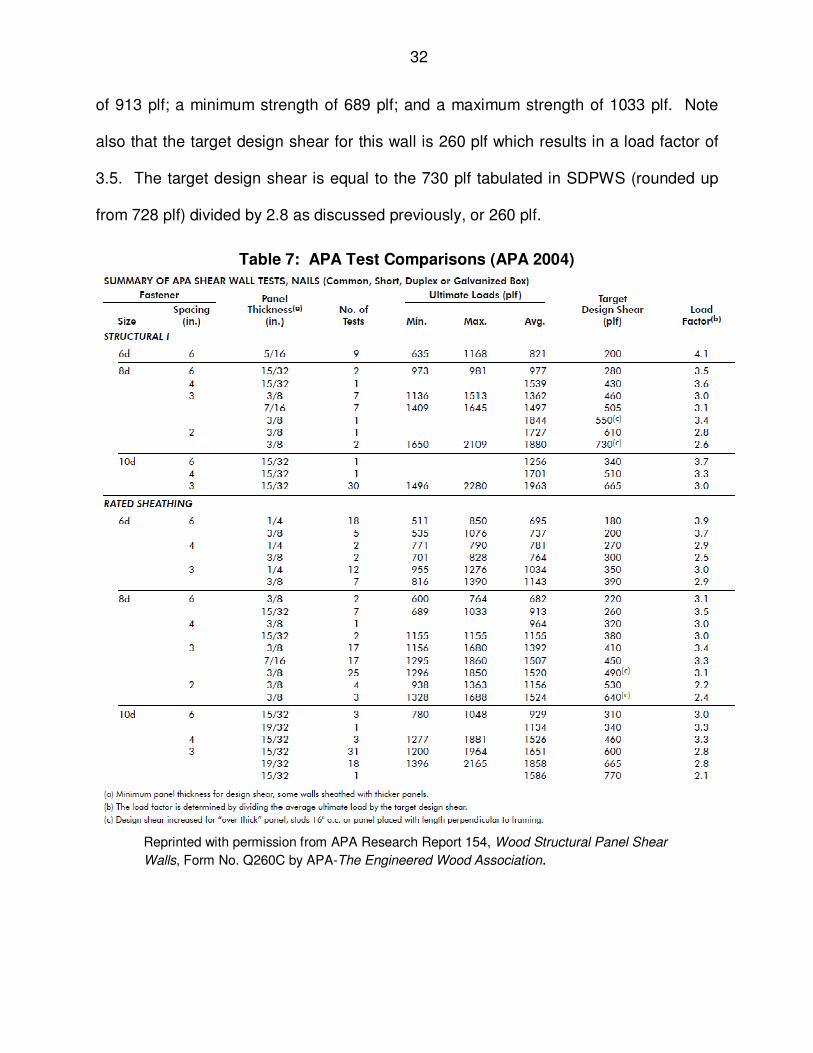
32
of 913 plf; a minimum strength of 689 plf; and a maximum strength of 1033 plf. Note
also that the target design shear for this wall is 260 plf which results in a load factor of
3.5. The target design shear is equal to the 730 plf tabulated in SDPWS (rounded up
from 728 plf) divided by 2.8 as discussed previously, or 260 plf.
Table 7: APA Test Comparisons (APA 2004)
Reprinted with permission from APA Research Report 154, Wood Structural Panel Shear
Walls, Form No. Q260C by APA-The Engineered Wood Association.

33
2.9 Shear Wall Strength and Computer Modeling
Shear wall strength can be either calculated (mechanistic) or determined from
testing (hysteresis). A mechanistic model is provided in APA Research Report 154
(2004) for determining the capacity of a fully restrained shear wall. This model is based
on the nail capacities in the NDS (2005). The mechanistic model simply resolves the
applied shear along the sole plate and the uplift force into the tension stud through the
fasteners in a unidirectional shear in the direction of the sole plate and tension chord
respectively. Cyclic testing is used to determine the nonlinear load-deformation
response of a shear wall. From this testing the hysteresis curves are produced. The
backbone curve, also referred to as the envelope curve, is formed from the peaks of the
hysteresis curves. The backbone curve, shown in Figure 5, closely approximates the
nonlinear load deformation curve produced from a monotonic test (van de Lindt 2003).
Figure 5: Hysteresis Curve Example
0.0
0.0
Backbone Curve

34
The CASHEW program was developed by CUREE (California Universities for
Earthquake Engineering) to predict the load-displacement response for cyclic and
monotonic loading (Folz and Filiatrault 2001). The program uses 10-parameter nail
data to define the hysteresis loop as shown in Figure 6. Nail data is used from other
research to define the 10 parameters (van de Lindt and Walz 2003).
Figure 6: Hysteretic Response of a Sheathing-to-Framing Connector
This program and model has been used in several seismic studies for shear wall
modeling. The program was altered to add pinching effects in a reliability model by
van de Lindt and Walz (2003).
It is also noted that the CASHEW User’s Manual provides an example comparing
it to tests performed by Durham. The CASHEW results for the monotonic loading were
26% greater the actual shear wall test result (Folz and Filiatrault 2000).
Folz and Filiatrault 2000

35
2.9.1 Finite Element Modeling
Several studies have been done using finite element
modeling (FEM) of wood shear walls. These studies have
evolved over the years and can be rather simplistic models
or more complex models that account for every connection
in the wall. The programs used for the finite element
include commercial programs such as ABAQUS and ANSYS. Others have developed
programs as well, such as SHWALL and CASHEW.
This work is best summarized by Cassidy (2002) and Judd (2005). The most
common models include beam elements for framing members, four and eight node
plane stress elements for sheathing, and two orthogonal nonlinear springs (or spring
pair), Figure 7, to model the connections from the sheathing to the framing members
(e.g. Dolan and Foschi 1991; Folz and Filiatrault 2001; Cassidy 2002; Judd 2005).
Of the referenced examples, Judd, using ABAQUS, created an oriented spring
pair as a user element. Judd recognized that for nonlinear springs, the bilinear spring
isn’t equivalent to a single one dimensional spring. For monotonic loading, the peak
load and displacement can be accurately calculated with a bilinear spring element.
However, the total energy absorbed by the system is not accurate with the bilinear
spring, since the load deformation curve does not completely represent the behavior of
the actual wall (Cassidy 2002). The increased resultant stiffness overestimates the total
energy absorbed.
The most common method of modeling the framing connections is with pinned
joints (e.g. Judd 2005, CASHEW). The results of these models reasonably match the
1
1’
Figure 7: Spring Pair

36
test walls that they were developed for, but this type of model doesn’t accurately
capture the actual behavior of the wall. Cassidy (2002) used another spring pair to
model the behavior of the stud to plate connection. The spring pair had differing
stiffness for the load direction.
Using a typical stud-to-plate connection of two 16d Common nails, Cassidy
(2002) used a lateral stiffness of 12,000 lb/in which corresponds to results published by
Dolan et. al. (1995). Cassidy (2002) found that this parameter had “very little effect on
the overall load-displacement response of the wall.” Cassidy (2002) used a nonlinear
vertical stiffness. For compression, a vertical stiffness of 41,000 lb/in was used which
corresponds to his reported test results for the crushing of the wood sole plate. Cassidy
then used a tension stiffness of 100 lb/in. This was an assumption by Cassidy. The
vertical tension stiffness of course relates to nails installed in the end grain of the stud
loaded in withdrawal. According to the NDS Commentary (AF&PA 2005), there can be
up to a 50% reduction in nail withdrawal strength into end grain, and coupling this with
seasoning, the values are deemed too unreliable and are prohibited. However, there is
definitely some resistance and stiffness in this connection; although not reported to the
author’s knowledge.
2.9.2 Sheathing Nail Modeling
Sheathing nail modeling is considered in two ways. The first is considering the
yield limit equations from the NDS (AF&PA 2005). The second is considering the load
deformation relationship of the fasteners. The latter is of interest for finite element
modeling while the former is helpful in the understanding of allowable nail capacities
published in the NDS.
37
2.9.2.1 NDS Yield Limit Equations
The yield limit equations in the NDS (AF&PA 2005) provide a method to calculate
nail connection strength based on limit states or modes of failure. The yield limit
equations are a mechanics based method. Technical Report 12 (AF&PA 1999)
expands on the yield limit equations used in the NDS (AF&PA 2005). The modes of
failure of a dowel-type connection are “uniform bearing under the fastener, rotation of
the fastener in the joint without bending, and development of one or more plastic hinges
in the fastener.” (AF&PA 1991). Technical Report 12 (AF&PA 1999) provides the basis
for calculating the ultimate nail capacity for each mode of failure by considering the
specific gravity of the material, the thickness of each member, any gap that may exist
between the members, and the yield strength of the fastener. This is not the failure
load, but is rather the ultimate load. The failure load occurs after the ultimate load is
reached.
For single shear, there are four modes of failure to consider, Figure 8. These
modes are briefly described and explained here. They are based on no gap between
the members. Additionally, Technical Report 12 (AF&PA 1999) provides methods for
calculating the failure load at the proportional limit, the 5% offset limit, and the ultimate
limit. Only the ultimate limit is presented here.

38
Reprinted with permission from Technical Report 12, General Dowel Equations for
Calculating Lateral Connections by the American Wood Council, Leesburg, VA
Figure 8: Connection Yield Modes

39
2.9.2.1.1 Mode Im and Is
The limit state for failure mode I is either wood bearing in the main member (Im)
or wood bearing in the side member (Is) with no rotation or yielding of the fastener.
Mode I strength is:
Im mm lqP = Eq. 4
Is ss lqP = Eq. 5
2.9.2.1.2 Mode II
The limit state for failure mode II is side and main member wood bearing with
rigid rotation of the fastener, but no yielding of the fastener. Mode II strength is:
II A
ACBBP
2
42 −+−= Eq. 6
where,
ms qqA
4
1
4
1+=
22ms ll
B += 44
22
mmss lqlqC −−=
2.9.2.1.3 Mode IIIm and IIIs
The limit state for failure mode III is either main member bearing and yielding of
the fastener in the side member (IIIm) or side member bearing and yielding of the
fastener in the main member (IIIs). Mode IIIm and IIIs strength is defined by Eq. 6 where,
IIIm ms qq
A4
1
2
1+=
2mlB =
4
2
mms
lqMC −−=
IIIs ms qq
A2
1
4
1+=
2slB =
mss M
lqC −−=
4
2
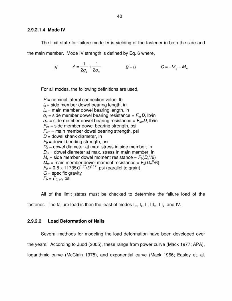
40
2.9.2.1.4 Mode IV
The limit state for failure mode IV is yielding of the fastener in both the side and
the main member. Mode IV strength is defined by Eq. 6 where,
IV ms qq
A2
1
2
1+= 0=B ms MMC −−=
For all modes, the following definitions are used,
P = nominal lateral connection value, lb ls = side member dowel bearing length, in lm = main member dowel bearing length, in qs = side member dowel bearing resistance = FesD, lb/in qm = side member dowel bearing resistance = FemD, lb/in Fes = side member dowel bearing strength, psi Fem = main member dowel bearing strength, psi D = dowel shank diameter, in Fb = dowel bending strength, psi Ds = dowel diameter at max. stress in side member, in Dm = dowel diameter at max. stress in main member, in Ms = side member dowel moment resistance = Fb(Ds
3/6) Mm = main member dowel moment resistance = Fb(Dm
3/6) Fe = 0.8 x 11735G1.07/D0.17, psi (parallel to grain) G = specific gravity Fb = Fb, ult, psi
All of the limit states must be checked to determine the failure load of the
fastener. The failure load is then the least of modes Im, Is, II, IIIm, IIIs, and IV.
2.9.2.2 Load Deformation of Nails
Several methods for modeling the load deformation have been developed over
the years. According to Judd (2005), these range from power curve (Mack 1977; APA),
logarithmic curve (McClain 1975), and exponential curve (Mack 1966; Easley et. al.
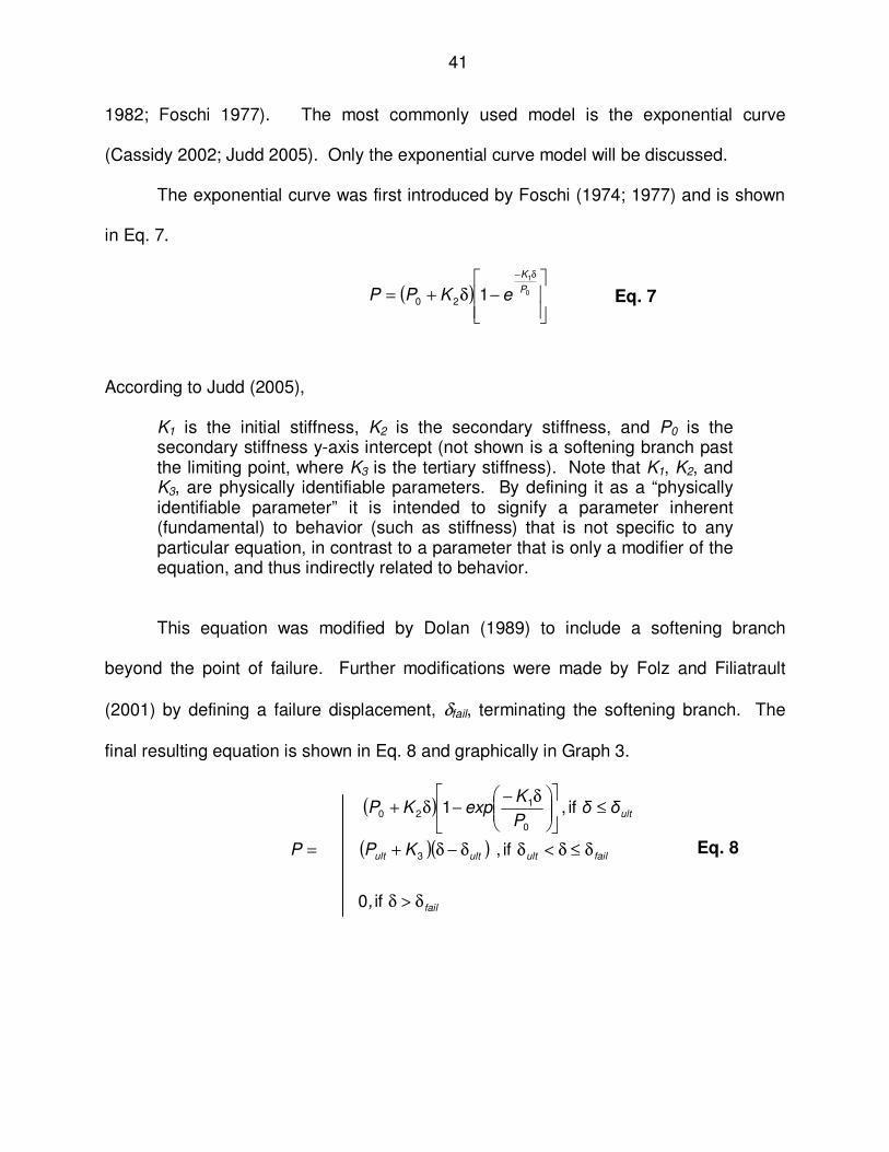
41
1982; Foschi 1977). The most commonly used model is the exponential curve
(Cassidy 2002; Judd 2005). Only the exponential curve model will be discussed.
The exponential curve was first introduced by Foschi (1974; 1977) and is shown
in Eq. 7.
( )
−δ+=
δ−
0
1
120P
K
eKPP Eq. 7
According to Judd (2005),
K1 is the initial stiffness, K2 is the secondary stiffness, and P0 is the secondary stiffness y-axis intercept (not shown is a softening branch past the limiting point, where K3 is the tertiary stiffness). Note that K1, K2, and K3, are physically identifiable parameters. By defining it as a “physically identifiable parameter” it is intended to signify a parameter inherent (fundamental) to behavior (such as stiffness) that is not specific to any particular equation, in contrast to a parameter that is only a modifier of the equation, and thus indirectly related to behavior.
This equation was modified by Dolan (1989) to include a softening branch
beyond the point of failure. Further modifications were made by Folz and Filiatrault
(2001) by defining a failure displacement, δfail, terminating the softening branch. The
final resulting equation is shown in Eq. 8 and graphically in Graph 3.
( )
( )( )
fail
failultultult
ult
,
KPP
δδP
KexpKP
δ>δ
δ≤δ<δδ−δ+=
≤
δ−−δ+
if 0
if ,
if , 1
3
0
120
Eq. 8
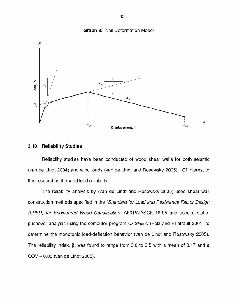
42
Graph 3: Nail Deformation Model
Displacement, in
Lo
ad
, lb
δδ ult
P
P o
K 1
1
K 2
1
K 3
1
δ fail
2.10 Reliability Studies
Reliability studies have been conducted of wood shear walls for both seismic
(van de Lindt 2004) and wind loads (van de Lindt and Rosowsky 2005). Of interest to
this research is the wind load reliability.
The reliability analysis by (van de Lindt and Rosowsky 2005) used shear wall
construction methods specified in the “Standard for Load and Resistance Factor Design
(LRFD) for Engineered Wood Construction” AF&PA/ASCE 16-95 and used a static-
pushover analysis using the computer program CASHEW (Folz and Filiatrault 2001) to
determine the monotonic load-deflection behavior (van de Lindt and Rosowsky 2005).
The reliability index, β, was found to range from 3.0 to 3.5 with a mean of 3.17 and a
COV = 0.05 (van de Lindt 2005).

43
Wind velocity is modeled as a Gumbel distribution or Type I (Ellingwood et al,
1980). This distribution is an extreme value distribution which is asymptotic with a
Cumulative Distribution Function (CDF) given as the double exponential function shown
in Eq. 9 (Ang and Tang 1975):
( ) ( )( )[ ] ∞<<∞−−α−−= xuxexpexpxFX Eq. 9
Although the wind velocity has a Type I distribution, this doesn’t necessarily mean that
the wind load has a Type I distribution since the wind load is a function of the velocity
squared. However, this relationship was studied considering the other random
variables (pressure coefficients, exposure factor and gust factor) that influence the wind
load and it was determined that the probability distribution of wind load is also a Type I
distribution (Ellingwood et al, 1980)
Van de Lindt used the model suggested by Ellingwood (1999). For this model,
the 50-year maximum wind load is modeled as a Type I random variable, shown in
Graph 4. The bias factor (mean-to-nominal value), including directionality effects, is
given by:
80.W
W
N
= Eq. 10
where, W = mean wind load WN = nominal (code-specified) wind load
The coefficient of variation is 0.35 (van de Lindt and Rosowsky 2005). Van de Lindt’s
model considered the capacity of the shear wall given in SDPWS multiplied by the
strength reduction factor, φ, (the load with a Type I distribution) as the random variable.
This was the only random variable used, since the resistance, computed as the ultimate

44
wall strength from CASHEW, was assumed to be deterministic as shown as the vertical
line in Graph 5.
Graph 4: Probability Density Function of Shear Wall Load
Van de Lindt used the limit state in its simplest form to calculate the second-
moment reliability index, β. This limit state is shown here as:
g(x) = R-S Eq. 11
where g(x) is the limit state function, R is the structural resistance, and S is the load
effect. R could be a random variable and S could be a random variable, or they could
be a function of several random variables. As noted earlier, van de Lindt chose to only
use S as a random variable and R as a constant (van de Lindt and Rosowsky 2005).
0 2 4 6 8 10 120
0.1
0.2
0.3
0.4
0.5
0
F x( )

45
For the limit state shown above, failure occurs when g(x) < 0. As shown in the shaded
portion of Graph 5, probability of failure, pf, is the probability that g(x) < 0.
Graph 5: Failure Region of PDF of Shear Wall Load
The reliability index, β, is the inverse of the standard normal distribution function
and is determined by:
( )fp−Φ=β − 11 Eq. 12
β, shown graphically on the standard normal distribution in Graph 6 is a scale of the
standard deviation, σ, to the probability of failure. This allows a measure of structural
safety for any limit state, material, or load.
Probability of Failure, pf g(x)

46
Graph 6: Reliability Index, β, on the Standard Normal Distribution
2.11 IRC Brace wall Testing - SBC Research Institute
The SBC Research Institute tested a 12’ x 30’ structure, Figure 9 and
Figure 10, with IRC prescriptive intermittent walls in early 2010. The test results are
currently available in the SBCRI Tech Note titled 2009 International Residential Code
(IRC) Braced Wall Panel Design Value Comparative Equivalency Testing – Braced Wall
Panel Design Values (TN-IRC WSP 2010).
A portion of the test results are summarized in Table 8. There are several items
of interest from this data. First, for the 3/8” WSP, the average ultimate unit shear
strength is 27% less than the IRC full restraint value and 8% less than the IRC value
assuming the 80% PR factor. Second, the location of the 7/16” WSP did not have much
of an effect on the strength of the wall. It was expected that the corners would have
more restraint and thus would have a greater capacity. Third, the average ultimate unit
shear of the 7/16” WSP with partial restraint is 18% less than the IRC full restraint value
βσ
pf
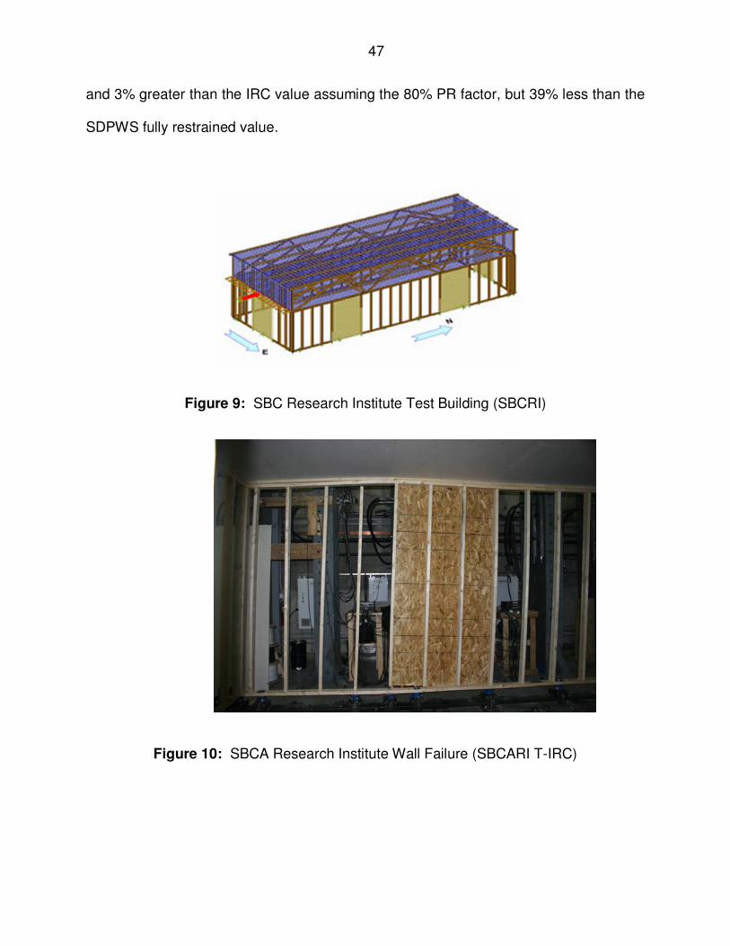
47
and 3% greater than the IRC value assuming the 80% PR factor, but 39% less than the
SDPWS fully restrained value.
Figure 9: SBC Research Institute Test Building (SBCRI)
Figure 10: SBCA Research Institute Wall Failure (SBCARI T-IRC)

48
Table 8: Summary of SBCRI Tests
Wall Sheathing Location
Restraint Average Ultimate Unit
Shear (plf)
IRC Full Restraint
(plf)
IRC with 80% PR Factor (plf)
IRC 3/8” WSP 6d
nails at 6/12
6’ From Corner
Partial – Building
Dead Load and IRC Anchors
367 500 400
IRC 7/16” WSP 8d
nails at 6/12
6’ From Corner
Partial – Building
Dead Load and IRC Anchors
412 500 400
IRC 7/16” WSP 8d
nails at 6/12 At Corner
Partial – Building
Dead Load and IRC Anchors
426 500 400
IRC 7/16” WSP 8d
nails at 6/12 with hold downs
6’ From Corner
Fully Restrained
626 6721 N.A.
1SDPWS value utilizing
15/32” and modified for G=0.42.
2.11.1 SBCRI Test Results
A comparison can be made between Seaders, SBCRI, and SDPWS modified by
Ni and Karacabeyli’s partial restraint factor, α. Recall that SBCRI test values are shown
in Table 8 while Seaders’ test results are shown in Table 5. Since Seaders’ test used
Douglas Fir-Larch, G=0.50, and the SBCRI used Spruce-Pine-Fir, G=0.42, the Seaders’
values are expected to be 8% greater. Also, Seaders added gypsum to the face of the
wall opposite the WSP with nominal fastening that added some additional strength.

49
Therefore, the comparison shown in Table 9 provides a quick view of the differences
without accounting for the construction differences.
The SDPWS values shown in Table 9 are modified by the partial restraint factor,
α, using Eq. 2. There is a 19% error for the unrestrained (actually greater if the gypsum
strength and Douglas Fir-Larch framing are considered) and a 23% error for the partially
restrained. A further comparison of Seaders’ results with the SDPWS modified by the
partial restraint factor, α, is shown in Table 10.
As shown in Table 10, the results of the fully restrained wall were not much
different than the SDPWS, 6.3% error. However, there is a large difference in the
Unrestrained (UR) and Partially Restrained (PR) values, 25.8% for UR and up to 36.2%
for PR. Therefore, it appears that the partial restraint factor, α, using Eq. 2 is not
accurate for IRC walls.
Table 9: Comparison of SBCRI, Seaders, SDPWS
FR UR PR
SBCRI 412Seaders 271
SDPWS 672 336 538% of FR 100% 40% 61%
Expected % of FR1
100% 50% 80%% Error N.A. 19.3% 23.4%
1IRC uses 0.8 for one story structure with 500 plf.
Table 10: Comparison of Seaders to SDPWS
FR UR 40% 49%
Seaders 684 271 383 509SDPWS 730 365 600 649% Error 6.3% 25.8% 36.2% 21.6%
PR

50
The inaccuracy of the partial restraint factor, α, is most likely due to the anchor
bolt locations. Recall that the IRC wall is anchored with ½” diameter anchor bolts a
maximum of 12” from the end and 6’ o.c. while Ni and Karacabeyli’s wall tests utilized
½” diameter anchor bolts at 16” o.c. and 8” from the ends. Therefore, some
modification of Eq. 2 is necessary for IRC anchored walls.
The capacity of an unrestrained 3/8” WSP shear wall constructed and anchored
according to the IRC is unknown at this time. If there is a correlation between the 7/16”
and the 3/8” WSP unrestrained, then the unrestrained value of the 3/8” WSP would be
40% of the SDPWS value or one half of the assumed 80% value that the IRC uses.
Therefore, for a lightly loaded wall, the reliability would be much less for the IRC brace
wall than the SDPWS fully restrained wall.

51
CHAPTER 3
TESTING OF SHEAR WALLS
This chapter summarizes the test procedure, test results and numerical data from
the testing of 25 wood shear walls. The 25 shear walls were divided into five groups of
five walls each. The restraint of the shear walls was set differently for all five sets to
understand the effect of partial restraint and full restraint on the shear wall unit shear
capacity.
3.1 Current ASTM Test Procedures
Two ASTM standards exist for shear wall testing. The first is the “Standard Test
Methods of Conducting Strength Tests of Panels for Building Construction” (ASTM
E72-10). The second is the “Standard Practice for Static Load Test for Shear
Resistance of Framed Walls for Buildings” (ASTM E564-00).
The purpose of ASTM E72 is to evaluate different types of sheathing on a
standard wood frame. Since the standard wood frame is the same for all sheathing
materials, the relative difference in performance of the sheathing materials is the test
objective (ASTM E72). Three tests are required by this standard. ASTM E72 employs
an 8’ x 8’ panel (two sheets of WSPs). The frame is constructed with 2x4 studs spaced
at 16” on center with a single 2x4 sole plate and a double 2x4 top plate. Spaced corner
posts are used at each end with fastening to the outside post only. All framing material
is No. 1 Douglas Fir or Southern Pine. Fastening of the WSPs shall follow the
manufacturer’s recommendations. The standard emphasizes the importance of placing
the fasteners exactly in the required location maintaining the correct edge distance and

52
angle (typically perpendicular to the WSP). Figure 11 shows the frame required by
ASTM E72.
Reprinted, with permission, from ASTM E72-10 “Standard Test Methods of Conducting Strength Tests of Panels for Building Construction”, copyright ASTM International, 100 Barr Harbor Drive, West Conshohocken, PA 49428.
Figure 11: Standard Wood Frame (ASTM E72)
ASTM E72 also specifies the loading point, the load rate, a hold down device,
and the points of measurement. The load point is at the end of a timber member bolted
to the double top plate. The hold down device consists of two steel rods extending
53
through a bearing plate with rollers above the corner post at the end where the load is
applied. The rods are installed such that one is located on each side of the frame. The
load rate specifies application of a uniform rate of motion to three steps: 790, 1570, and
2360 lb. The load shall be applied at the same rate for all three steps, but the first step
must be loaded in no more than two minutes. Upon reaching the first load step,
measurements are made at each measurement point and then the wall is unloaded.
Measurements are again made after unloading to determine any permanent
deformation. This process is repeated for the next two load steps. Three points of
measurement are required for this test. They are all horizontal measurements. One
point is located at the end of the double top plate and the remaining two are located at
each end of the sole plate. The displacement measurements must be recorded to the
nearest 0.01”
The purpose of ASTM E564 is to evaluate the shear capacity of any type of light
framed wall supported on a rigid foundation and to determine the shear stiffness and
strength of the wall (ASTM E564). The standard does not dictate a particular hold down
device, but rather specifies the use of the same anchorage and applied axial loads
expected in the service condition. Similarly, the framing members and fastening shall
be the same size, grade and construction as anticipated in actual use.
ASTM E564 also specifies loading requirements. Although similar to ASTM
E72, there are some slight differences between the standards. ASTM E564 requires an
initial load equal to 10% of the anticipated ultimate load to be applied for five minutes to
seat all connections. The initial load is removed and after five minutes the initial
readings of displacement are recorded. The next sequence of loading is then applied in

54
intervals, or load steps, of 1/3, 2/3, and finally, the ultimate load. All of the load steps
are applied at the same rate which is equal to reaching the anticipated ultimate load in
no less than five minutes. At each of these intervals the load step is applied up to the
specified load and held for one minute. The displacements are then recorded, and then
the specimen is unloaded. After five minutes of unloading, the displacements are again
recorded. The process is then repeated until the last load step and ultimate failure is
reached. Ultimate failure may be a displacement limit rather than a load limit.
ASTM E564 provides a method for reporting both the global shear stiffness of the
wall and the internal shear stiffness of the wall as well as the ultimate strength. The
internal shear stiffness of the wall does not include uplift, or rotation, of the entire wall,
but rather only the distortion of the wall itself. The ultimate strength is reported as an
ultimate unit shear strength which is simply the ultimate load divided by the wall width.
ASTM E564 requires testing a minimum of two wall assemblies. If after testing
two assemblies either the shear stiffness or the ultimate strength are not within 15% of
each other, then a third test is required. The strength and stiffness values reported are
then the average of the two weakest specimen values.
3.2 Wall Testing
The following summarizes the test procedure and results of the 25 wood shear
walls used for the reliability analysis. The shear wall testing was conducted at the
Structural Building Components Research institute in Madison, WI in March 2011. The
tests were performed in accordance with ASTM E564. Details of the testing are
presented in Appendix A.

55
3.2.1 Test Facility
The SBCRI test facility has an ACLASS accreditation, Appendix B. ACLASS is
one of two brands of the ANSI-ASQ National Accreditation Board. The accreditation is
for testing full scale construction assemblies and is accredited to ISO/IEC 14025:2005.
Of particular interest, the accreditation specifically encompasses ASTM E564 and
ASTM E72 testing.
The SBCRI test facility is capable of testing both single components and entire
structures up to 30’ wide x 32’ tall x 90’ long. Completely adjustable frames allow for a
large variation of test configurations.
3.2.2 Wall Construction
3.2.2.1 Wall Matrix
The 25 shear walls were constructed identically, except for the anchorage, and
tested identically. The shear walls were grouped in five groups of five walls each for the
testing. See Table 11 for a summary of walls tested. Illustrations of the test setups are
shown in Figure 12, Figure 13, and Figure 14 at the end of this chapter.
Group A walls were tested first to determine the hold down force. The average
hold down force was used to calculate the restraining force for Groups B to D. More
details of the test program are presented in Appendix A.

56
Table 11: Test Matrix
Group A B C D E
No. of Tests 5 5 5 5 5 Size 4’x8’ 4’x8’ 4’x8’ 4’x8’ 4’x8’
OSB Sheathing Thickness
15/32” 15/32”
15/32” 15/32”
15/32”
2x4 Plate Material
Stud Grade SPF-S
Stud Grade SPF-S
Stud Grade SPF-S
Stud Grade SPF-S
Stud Grade SPF-S
2x4 Stud Material
#2 Grade SPF-N
#2 Grade SPF-N
#2 Grade SPF-N
#2 Grade SPF-N
#2 Grade SPF-N
2x4 Stud Spacing
16” 16” 16” 16” 16”
8d Common Nail Spacing
6:12 6:12 6:12 6:12 6:12
Restraint Mechanical Hold down
1104 lb (¼ Hold
Down Force)
2208 lb (½ Hold
Down Force)
3312 lb (¾ Hold
Down Force)
No added restraint
Anchor Bolt None 5/8” 12” from load edge
5/8” 12” from load edge
5/8” 12” from load edge
5/8”12” from load edge
3.3 Test Results
3.3.1 Data Results
The hysteresis curve for a typical wall tested to failure is shown in Graph 7.
From the test results, the ultimate unit shear capacity of each wall was found. A
summary of these results is shown in Table 12, including the average hold down force
for wall Group A. The restraining force shown for wall groups B, C, and D is ¼, ½, and
¾ of the average hold down force from Group A. The SDPWS value was determined
from the tabulated 730 plf which reduces to 628 plf for SPF-S (G=0.36). The Report
154 value was determined from APA Report 154 which tabulates an average fully
restrained ultimate unit shear capacity of 913 plf, which reduces to 786 plf for SPF-S
(G=0.36). The species reduction factor is (1-(0.5-0.36)) = 0.86. The restraining force for

57
SDPWS and APA Research Report 154 is the unit shear multiplied by the wall height of
8 feet. The normalized section indicates the fraction of the fully restrained hold down
force, calculated from the APA Research Report 154 average ultimate unit shear value,
and the resulting fraction of the Report 154 ultimate value.
Graph 7: Hysteresis Curve for Wall A1
0
500
1000
1500
2000
2500
0 0.5 1 1.5 2 2.5 3 3.5 4 4.5
Displacement, in
Lo
ad
, lb
Wall A1
The load deformation curves tor the five different wall sets were averaged (Graph
8). Note the difference in the behavior of Wall A, the wall type with a mechanical hold
down, compared with the other partially restrained walls. Also note that there is nearly a
linear relationship between the peaks of Wall B, Wall C, and Wall D - the three walls
with an applied dead load for restraint. Considering Walls B-E, the relationship is no
longer linear, as illustrated in Graph 8.
In addition to the wall ultimate unit shear capacity and hysteresis curve, the load-
deformation curves for the nails were also created for Group A as shown in Graph 9.
These curves were derived from the calculated differential displacement between the
Backbone Curve

58
Table 12: Summary of Wall Ultimate Unit Shear Capacity
A B C D E SDPWS Report 154 Wall
Restraint 4416 1104 2208 3312 0 5024 6288
Ultimate Capacity, plf
1 569 314 502 607 190 2 538 337 500 656 181 3 562 323 474 594 158 4 549 372 516 590 142 5 558 377 489 628 137
Avg. 555 345 496 615 162 628 786 Std. Dev. 12 29 16 27 23
COV 0.022 0.083 0.032 0.044 0.145 Min. 538 314 474 590 137 Max. 569 377 516 656 190
Normalized
Phold down 0.702 0.176 0.351 0.527 0.000 1
Vcap(%) 0.706 0.438 0.631 0.782 0.206 1
Graph 8: Summary of Wall Tests
Comparison of Walls
(Average Values)
R2 = 0.9852
0
100
200
300
400
500
600
700
-0.50 0.00 0.50 1.00 1.50 2.00 2.50 3.00 3.50 4.00 4.50
Displacement, inches
Lo
ad
, lb
/ft
Wall A
Wall B
Wall C
Wall D
Wall E
Linear Regression of
Peak of Walls B-D
Relationship of peak
capacities.

59
Graph 9: 8d Common Nail Curves from Wall Group A
Nail Load Deformation Curves
0
50
100
150
200
250
300
0.000 0.250 0.500 0.750 1.000 1.250
Displacement, in
Lo
ad
, lb
A1 Horizontal Nail
A2 Horizontal Nail
A3 Horizontal Nail
A4 Horizontal Nail
A5 Horizontal Nail
A1 Vertical Nail
A2 Vertical Nail
A3 Vertical Nail
A4 Vertical Nail
A5 Vertical Nail
OSB sheathing and the studs from the test results. The load was calculated by dividing
the force in the stud or plate by the effective number of nails along that member. The
effective number of nails considered only a portion of the corner nails, assuming that
they were directed to the center of the wall. This is reasonable since the nails are
loaded primarily in one direction in a shear wall restrained with a hold down. “The wall
specimen, as a whole, will experience the ‘average’ nail behavior.” wrote Dolan and
Madsen 1992. The curves were created for both the nails in the bottom plate as well as
the nails in the tension or compression end stud, depending upon which stud
experienced nail failure. The dominant failure of the walls was nail failure along the
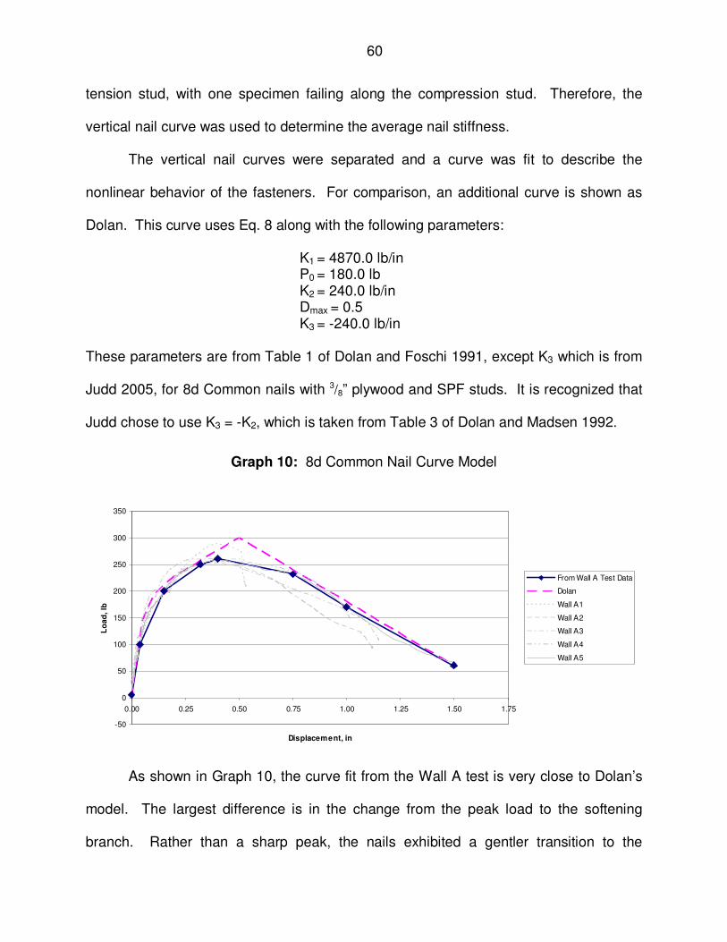
60
tension stud, with one specimen failing along the compression stud. Therefore, the
vertical nail curve was used to determine the average nail stiffness.
The vertical nail curves were separated and a curve was fit to describe the
nonlinear behavior of the fasteners. For comparison, an additional curve is shown as
Dolan. This curve uses Eq. 8 along with the following parameters:
K1 = 4870.0 lb/in P0 = 180.0 lb K2 = 240.0 lb/in Dmax = 0.5 K3 = -240.0 lb/in
These parameters are from Table 1 of Dolan and Foschi 1991, except K3 which is from
Judd 2005, for 8d Common nails with 3/8” plywood and SPF studs. It is recognized that
Judd chose to use K3 = -K2, which is taken from Table 3 of Dolan and Madsen 1992.
Graph 10: 8d Common Nail Curve Model
-50
0
50
100
150
200
250
300
350
0.00 0.25 0.50 0.75 1.00 1.25 1.50 1.75
Displacement, in
Lo
ad
, lb
From Wall A Test Data
Dolan
Wall A1
Wall A2
Wall A3
Wall A4
Wall A5
As shown in Graph 10, the curve fit from the Wall A test is very close to Dolan’s
model. The largest difference is in the change from the peak load to the softening
branch. Rather than a sharp peak, the nails exhibited a gentler transition to the
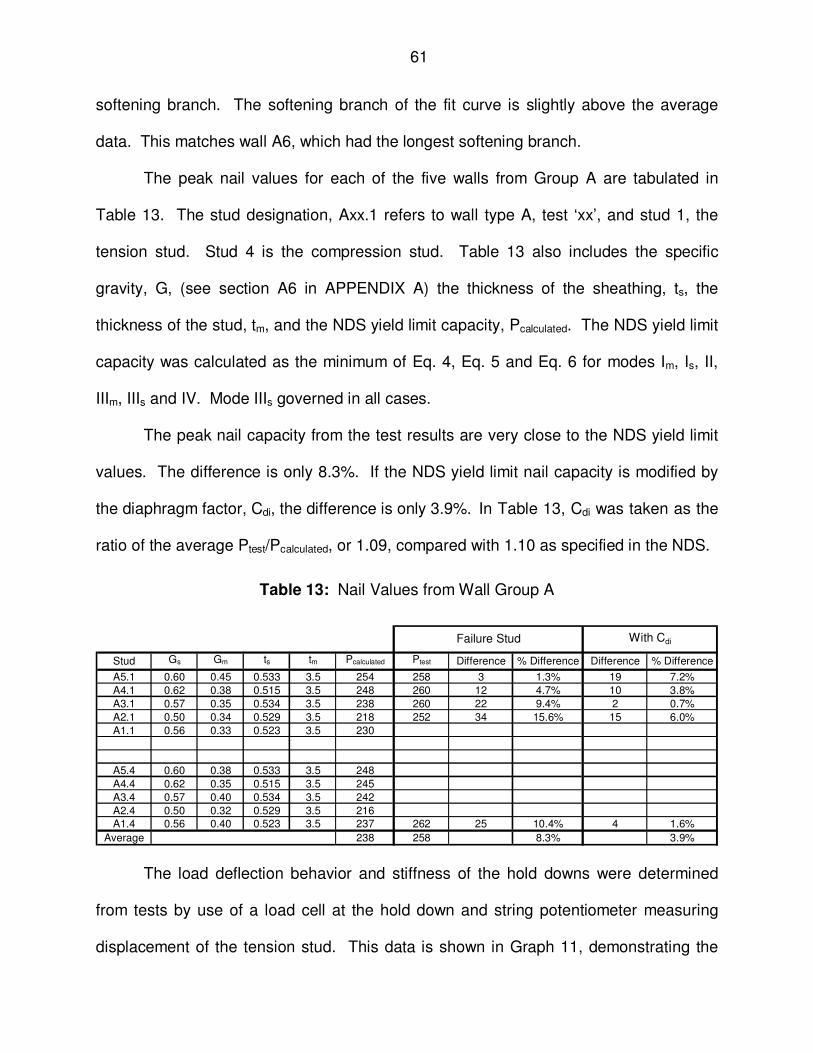
61
softening branch. The softening branch of the fit curve is slightly above the average
data. This matches wall A6, which had the longest softening branch.
The peak nail values for each of the five walls from Group A are tabulated in
Table 13. The stud designation, Axx.1 refers to wall type A, test ‘xx’, and stud 1, the
tension stud. Stud 4 is the compression stud. Table 13 also includes the specific
gravity, G, (see section A6 in APPENDIX A) the thickness of the sheathing, ts, the
thickness of the stud, tm, and the NDS yield limit capacity, Pcalculated. The NDS yield limit
capacity was calculated as the minimum of Eq. 4, Eq. 5 and Eq. 6 for modes Im, Is, II,
IIIm, IIIs and IV. Mode IIIs governed in all cases.
The peak nail capacity from the test results are very close to the NDS yield limit
values. The difference is only 8.3%. If the NDS yield limit nail capacity is modified by
the diaphragm factor, Cdi, the difference is only 3.9%. In Table 13, Cdi was taken as the
ratio of the average Ptest/Pcalculated, or 1.09, compared with 1.10 as specified in the NDS.
Table 13: Nail Values from Wall Group A
Stud Gs Gm ts tm Pcalculated Ptest Difference % Difference Difference % Difference
A5.1 0.60 0.45 0.533 3.5 254 258 3 1.3% 19 7.2%
A4.1 0.62 0.38 0.515 3.5 248 260 12 4.7% 10 3.8%
A3.1 0.57 0.35 0.534 3.5 238 260 22 9.4% 2 0.7%
A2.1 0.50 0.34 0.529 3.5 218 252 34 15.6% 15 6.0%
A1.1 0.56 0.33 0.523 3.5 230
A5.4 0.60 0.38 0.533 3.5 248
A4.4 0.62 0.35 0.515 3.5 245
A3.4 0.57 0.40 0.534 3.5 242
A2.4 0.50 0.32 0.529 3.5 216A1.4 0.56 0.40 0.523 3.5 237 262 25 10.4% 4 1.6%
Average 238 258 8.3% 3.9%
With CdiFailure Stud
The load deflection behavior and stiffness of the hold downs were determined
from tests by use of a load cell at the hold down and string potentiometer measuring
displacement of the tension stud. This data is shown in Graph 11, demonstrating the
62
slip that occurs before the linear behavior of the hold down is achieved. Note that walls
A1 through A4 utilized a Simpson HDU14 while wall A5 utilized a Simpson HDU8.
While the stiffness of the HDU14 is consistent, the slip varies. Unexpectedly, the HDU8
was stiffer than the HDU14.
Holdown Stiffness
0
500
1000
1500
2000
2500
3000
3500
4000
4500
5000
0.00 0.05 0.10 0.15 0.20 0.25 0.30 0.35
Displacement, inches
Lo
ad
, lb
Wall A1
Walll A2
Wall A3
Wall A4
Wall A5
Graph 11: Hold down Stiffness from Test Results
3.3.2 Discussion of Wall Failures
Nearly all of the walls failed as expected. The failure mode of four of the test
specimens, walls A2, A3, A4, and A5 in wall Group A, was nail failure along the tension
stud. The failure mode of one wall from wall Group A, wall A1, was nail failure along the
compression stud.
The nails typically failed in mode IIIs with some in mode IV, Figure 8. The IIIs
mode failure is a single yielding of the nail along with rotation of the nail in the
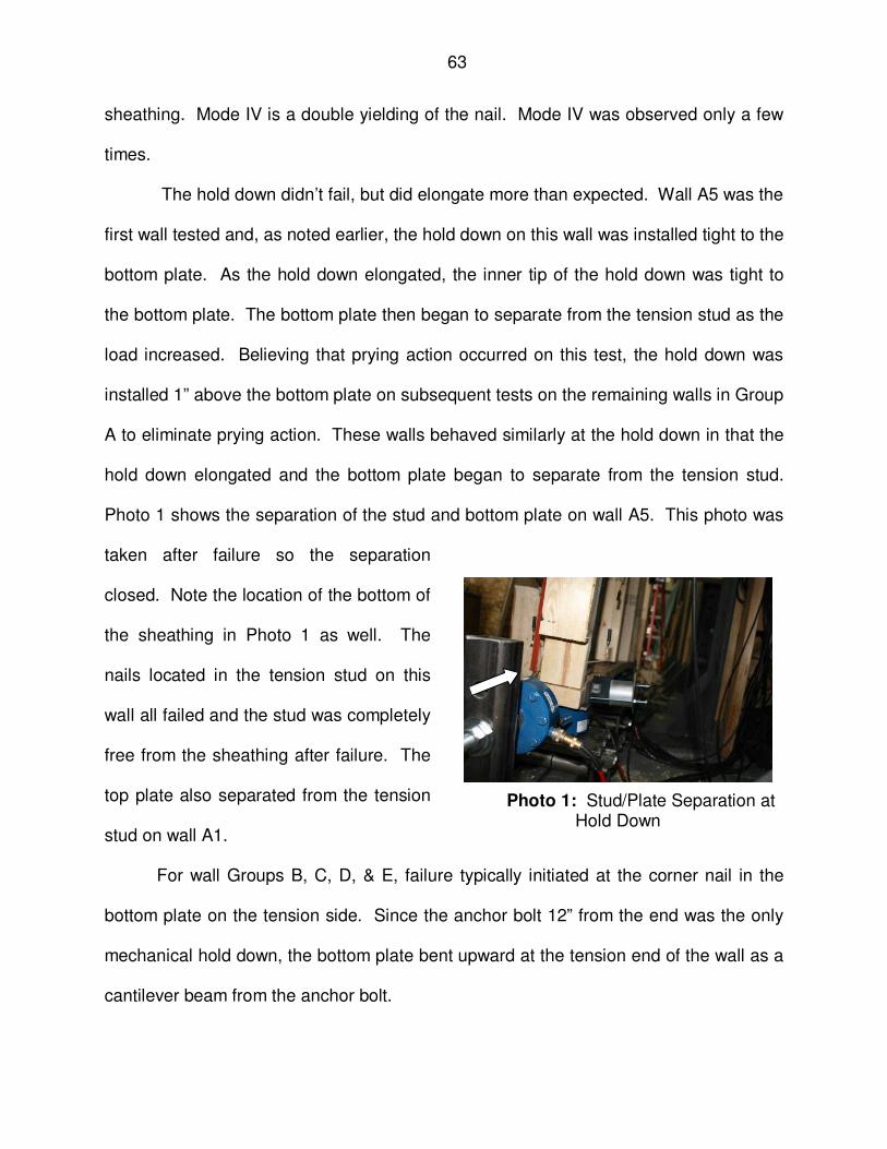
63
sheathing. Mode IV is a double yielding of the nail. Mode IV was observed only a few
times.
The hold down didn’t fail, but did elongate more than expected. Wall A5 was the
first wall tested and, as noted earlier, the hold down on this wall was installed tight to the
bottom plate. As the hold down elongated, the inner tip of the hold down was tight to
the bottom plate. The bottom plate then began to separate from the tension stud as the
load increased. Believing that prying action occurred on this test, the hold down was
installed 1” above the bottom plate on subsequent tests on the remaining walls in Group
A to eliminate prying action. These walls behaved similarly at the hold down in that the
hold down elongated and the bottom plate began to separate from the tension stud.
Photo 1 shows the separation of the stud and bottom plate on wall A5. This photo was
taken after failure so the separation
closed. Note the location of the bottom of
the sheathing in Photo 1 as well. The
nails located in the tension stud on this
wall all failed and the stud was completely
free from the sheathing after failure. The
top plate also separated from the tension
stud on wall A1.
For wall Groups B, C, D, & E, failure typically initiated at the corner nail in the
bottom plate on the tension side. Since the anchor bolt 12” from the end was the only
mechanical hold down, the bottom plate bent upward at the tension end of the wall as a
cantilever beam from the anchor bolt.
Photo 1: Stud/Plate Separation at Hold Down
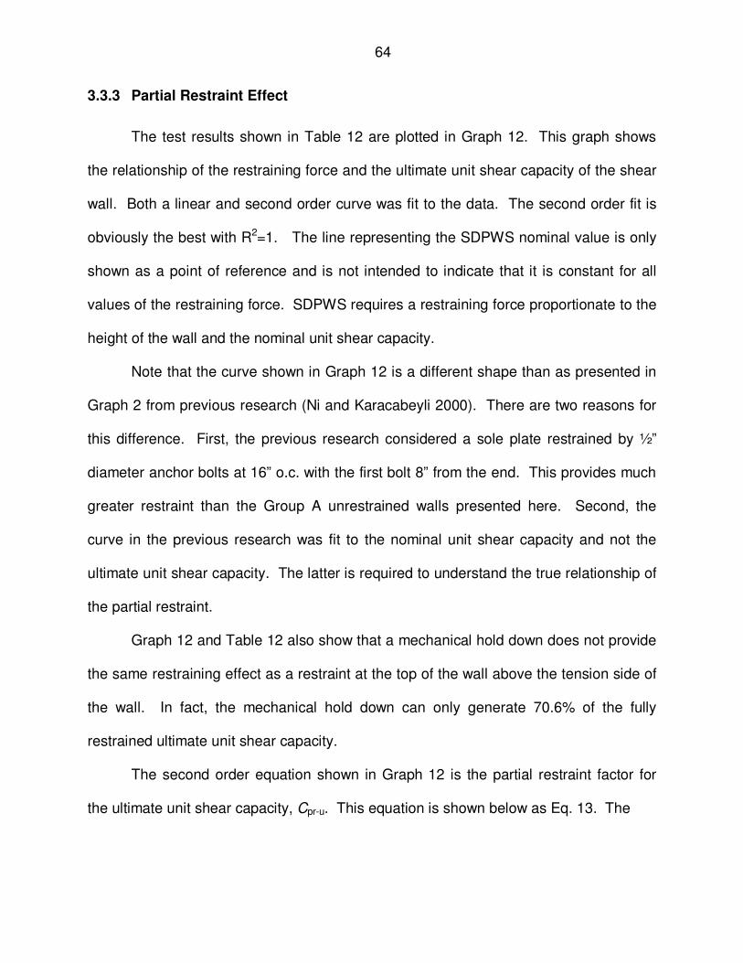
64
3.3.3 Partial Restraint Effect
The test results shown in Table 12 are plotted in Graph 12. This graph shows
the relationship of the restraining force and the ultimate unit shear capacity of the shear
wall. Both a linear and second order curve was fit to the data. The second order fit is
obviously the best with R2=1. The line representing the SDPWS nominal value is only
shown as a point of reference and is not intended to indicate that it is constant for all
values of the restraining force. SDPWS requires a restraining force proportionate to the
height of the wall and the nominal unit shear capacity.
Note that the curve shown in Graph 12 is a different shape than as presented in
Graph 2 from previous research (Ni and Karacabeyli 2000). There are two reasons for
this difference. First, the previous research considered a sole plate restrained by ½”
diameter anchor bolts at 16” o.c. with the first bolt 8” from the end. This provides much
greater restraint than the Group A unrestrained walls presented here. Second, the
curve in the previous research was fit to the nominal unit shear capacity and not the
ultimate unit shear capacity. The latter is required to understand the true relationship of
the partial restraint.
Graph 12 and Table 12 also show that a mechanical hold down does not provide
the same restraining effect as a restraint at the top of the wall above the tension side of
the wall. In fact, the mechanical hold down can only generate 70.6% of the fully
restrained ultimate unit shear capacity.
The second order equation shown in Graph 12 is the partial restraint factor for
the ultimate unit shear capacity, Cpr-u. This equation is shown below as Eq. 13. The

65
y = 0.7735x + 0.2939R² = 0.9378
y = -0.6393x2 + 1.4331x + 0.206R² = 1
0%
20%
40%
60%
80%
100%
120%
0% 20% 40% 60% 80% 100% 120%
% o
f F
ull S
he
ar
Cap
ac
ity
% of Full Restraining Force, λλλλ
Test Data + APA
Holdown
SDPWS Nominal
Linear (Test Data + APA)
Poly. (Test Data + APA)
Linear Fit
Second Order Fit
Graph 12: Partial Restraint Effect on Strength
ultimate unit shear capacity of a partially restrained wall can now be determined from
Eq. 14:
Cpr-u = -0.6393λ2+1.4331λ+0.206 ≤ 1.0 and Cpr-u = 0.706 for a mechanical hold down
Eq. 13
Where,
height wallshearh
capacity shear unit ultimateV
force grestraininP
hV
P
ult
D
ult
D
=
=
=
×=λ
Vpr=Cpr-uVult Eq. 14
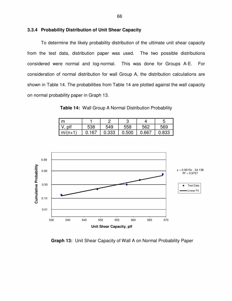
66
3.3.4 Probability Distribution of Unit Shear Capacity
To determine the likely probability distribution of the ultimate unit shear capacity
from the test data, distribution paper was used. The two possible distributions
considered were normal and log-normal. This was done for Groups A-E. For
consideration of normal distribution for wall Group A, the distribution calculations are
shown in Table 14. The probabilities from Table 14 are plotted against the wall capacity
on normal probability paper in Graph 13.
Table 14: Wall Group A Normal Distribution Probability
m 1 2 3 4 5
V, plf 538 549 558 562 569 m/(n+1) 0.167 0.333 0.500 0.667 0.833
0.01
0.10
0.50
0.90
0.99
y = 0.0615x - 34.138R² = 0.9757
535 540 545 550 555 560 565 570
Cu
mu
lati
ve
Pro
bab
ilit
y
Unit Shear Capacity, plf
Test Data
Linear Fit
Graph 13: Unit Shear Capacity of Wall A on Normal Probability Paper

67
For consideration of log-normal distribution for wall Group A, the distribution calculations
shown in Table 14 are plotted against the wall capacity on log-normal probability paper
in Graph 14.
0.01
0.10
0.50
0.90
0.99
520 540 560 580 600
y = 0.0615x - 34.138R² = 0.9757
500
Cu
mu
lati
ve P
rob
ab
ilit
y
Unit Shear Capacity, plf
Test Data
Linear Fit
Graph 14: Unit Shear Capacity of Wall A on Log-Normal Probability Paper
While both graphs indicate a close fit and very similar result (equation of the line
is the same for both and R2 is the same for both), log-normal distribution will be used.
Log-normal distribution does not allow negative values, so it is preferred over normal
distribution. The remaining walls resulted in similar conclusions.
The Chi-square test is another method for determining the best matching
distribution. However, a Chi-square test should have a minimum of 25-30 samples and
at least five bins (Ang & Tang 1975). Since the sample size is only five, it is not feasible
to use the Chi-square test for this data.
Similarly, another goodness-of-fit test is the Kolmogorov-Smirnov test for
distribution. With having only five samples, the results of this test are the same for

68
normal and log-normal distribution at the 5% significance level. Thus no conclusions
can be made from the K-S test.
3.3.5 Probability Distribution of Specific Gravity
Samples of each member were taken from the test specimens and specific
gravity tests were conducted for each piece in accordance with ASTM 2395. The
results of the test are shown in section A6 in APPENDIX A and summarized in Table
15.
Two distributions for specific gravity were considered, normal and log-normal.
The two distributions were compared with a Chi-Squared Test. Although both were
valid distributions, log-normal was selected because it always yields a positive value.
Table 15: Summary of Specific Gravity Tests
Member Studs Plates Sheathing
Description 2x4 Stud Grade SPF-S
No. 2 Grade SPF-N
15/32” OSB
Number of Pieces Tested
100 75 25
Exp. Ref. Exp. Ref. Exp. Ref.
Average, G 0.36 0.361 0.40 0.421 0.58 0.503 Std. Dev. 0.03 0.0362 0.03 0.0422 0.03 Specific Gravity
Prob. Dist Log-normal Log-normal Log-normal
Average, MC 15.1% 16.2% 4.7% Moisture Content Std. Dev. 1.5%
2.1%
0.4%
Average, t (in) 0.511 Thickness
Std. Dev.
0.017 Exp. = Experimental Value; Ref. = Reference Value 1 NDS (2005)
2 ASTM D2555 – 06
3 PDS (2004)

69
3.3.6 Wall Restrained with Hold Down
The ultimate unit shear strengths were calculated using the APA Research
Report 154 (2004) tabulated average ultimate value along with the modification required
for specific gravity, as shown in footnote C of Table 6, using the weighted average of
the specific gravity of the actual materials. The calculated results were compared with
the test values for Group A walls and are tabulated in Table 16 and shown in Graph 15.
The results were good with an average percent error of 0.07% between the
average experimental values and the average calculated values. As seen in both Table
16 and Graph 15, walls A3, A4, and A5 were the most consistent to their respective
anticipated values with an average percent error of -0.6%. Walls A1 and A2 are the
outlying values producing percent errors of 5.1% and 2.8% respectively.
Graph 15 illustrates the correlation between the wall unit shear capacity and the
average specific gravity of the wall framing members. The test results are compared
against the expected values calculated from the APA Research Report 154 (2004)
tabulated average ultimate value along with the modification required for a specific
gravity. The bandwidth shown is ±σ, or one standard deviation, of the experimental wall
capacity. All but wall A1 lie within the bandwidth.
Although a linear regression of the results from walls A1 to A5 do not correspond
to the expected relationship of the wall unit shear strength to the specific gravity, G, the
data fits relatively well within the bandwidth. This result can be expected with a small
sample size.

70
Table 16: Effectiveness of Hold Down
Wall
A1 0.344 569 771 0.702 541 5.1%A2 0.363 538 788 0.702 553 -2.8%
A3 0.379 562 802 0.702 564 -0.3%A4 0.364 549 789 0.702 554 -0.9%A5 0.377 558 800 0.702 562 -0.7%
Average 0.373 556 797 0.702 560 -0.6%Std. Dev. 6.7
Average 0.365 555 790 0.702 555 0.07%Std. Dev. 0.0137 12.0 8.8
Walls A1, A2, A3, A4, and A5
% Error
Gave
Plates and
Studs
Holdown
Reduction
APA
Report 154
Capacity
APA Report
154
Adjusted for
Holdown
Experimental
Wall Capacity
Walls A3, A4, and A5
Graph 15: Correlation of Wall Strength to Specific Gravity
0
100
200
300
400
500
600
700
0.340 0.350 0.360 0.370 0.380 0.390
Average Specific Gravity of Wall Studs and Plates, G
Wall
Str
en
gth
, p
lf
Wall A Test Values
Adjusted APA 154
+σ
−σ

Figure 12: Test Assembly Wall A
71

Figure 13: Test Assembly Walls B, C and D
72

Figure 14: Test Assembly Wall E
73

74
CHAPTER 4
FINITE ELEMENT MODELING
A finite element model was created to offer a better understanding of the
behavior of the walls with varying restraint conditions. The model includes a nonlinear
finite element analysis. The load deformation curves are compared to the test results
for accuracy of the model.
4.1 Finite Element Model
The finite element model (FEM) was constructed in HYPERMESH and analyzed
in ABAQUS, a commercial finite element solver. The model was constructed to
replicate as much detail as possible of the walls tested. The model used:
• Beam elements for the framing members • Four node quadrilateral shell elements • Two orthogonal springs connecting framing members, one linear and one
nonlinear • Two uncoupled orthogonal nonlinear springs (or spring pair) connecting
the sheathing to the framing elements • Compression-only beam elements at the supports that cannot resist
tension • And a nonlinear spring for the hold down.
Initially, the model was constructed with a single 1D nonlinear spring element
that was free to rotate (a SpringA element in ABAQUS). However, this element created
difficulties solving. It was extremely difficult to obtain convergence in the early steps of
the analysis. ABAQUS had difficulty in these early steps as the springs rotated to their
initial displacement path. The uncoupled nonlinear spring pair overcame this difficulty
and created a model that was easier to converge during the initial steps.
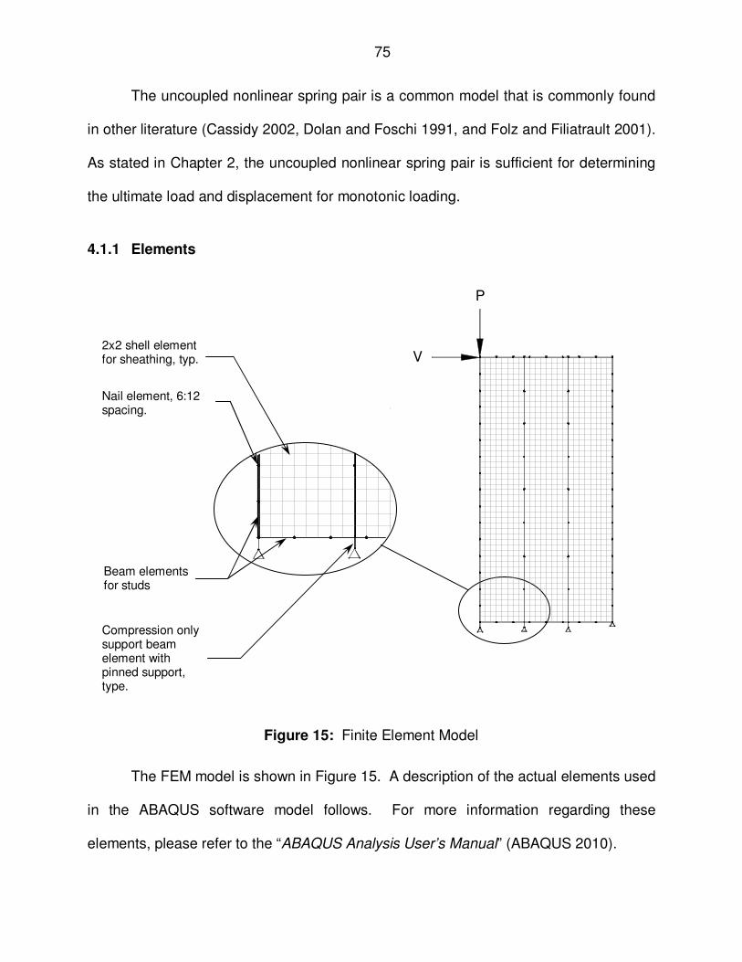
75
The uncoupled nonlinear spring pair is a common model that is commonly found
in other literature (Cassidy 2002, Dolan and Foschi 1991, and Folz and Filiatrault 2001).
As stated in Chapter 2, the uncoupled nonlinear spring pair is sufficient for determining
the ultimate load and displacement for monotonic loading.
4.1.1 Elements
Figure 15: Finite Element Model
The FEM model is shown in Figure 15. A description of the actual elements used
in the ABAQUS software model follows. For more information regarding these
elements, please refer to the “ABAQUS Analysis User’s Manual” (ABAQUS 2010).
Nail element, 6:12 spacing.
V
P
2x2 shell element for sheathing, typ.
Compression only support beam element with pinned support, type.
Beam elements for studs

76
4.1.1.1 Framing Members
The framing members, studs and plates were modeled as type B31 two node
three-dimensional beam elements. This element uses linear interpolation. B31
elements have six degrees of freedom at each end. These elements can be defined by
different geometric shapes. For this model, a rectangular shape was used to model a
2x4 framing member.
The second top plate of the wall was fastened only to the first top plate of the
wall. This was deemed insignificant to the strength and stiffness of the wall since it was
not fastened to the sheathing. It is common for models in the literature (Cassidy 2002,
Judd 2005) to use both plates as one member of equal dimension. This would create
additional stiffness that does not exist for the walls tested in this research.
Material properties for the B31 element are defined in the material properties
card. The material properties used are explained in the Materials section of this chapter.
The length of the elements for the studs was 6” and the length of the elements
for the sole and top plate was 2”. These lengths worked well for the nail and framing
geometry and for the behavior of the wall as well.
4.1.1.2 Nails
The framing members were connected with two orthogonal springs (or spring
pair), one linear and one nonlinear, as shown in Figure 16. As noted earlier, these
springs are each one dimensional spring elements. These springs are modeled as
Spring2 elements in ABAQUS. The spring used for lateral movement, or shear, was a
linear spring while the spring used for end grain withdrawal was a nonlinear spring.
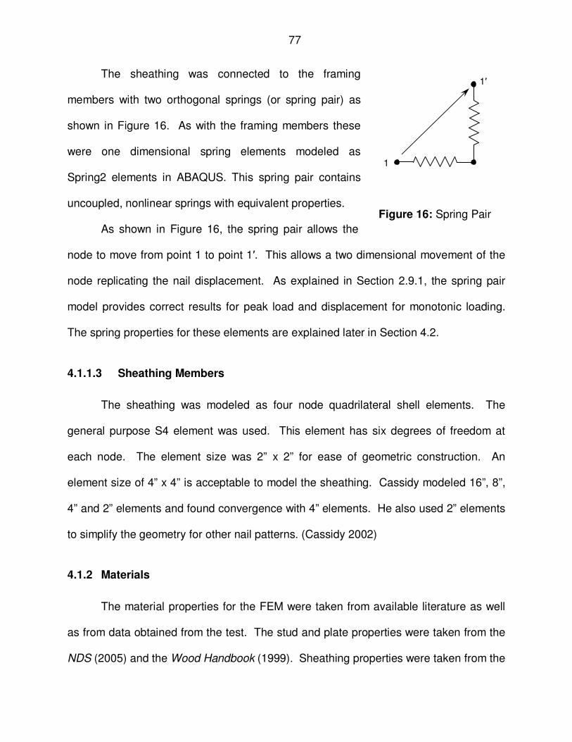
77
The sheathing was connected to the framing
members with two orthogonal springs (or spring pair) as
shown in Figure 16. As with the framing members these
were one dimensional spring elements modeled as
Spring2 elements in ABAQUS. This spring pair contains
uncoupled, nonlinear springs with equivalent properties.
As shown in Figure 16, the spring pair allows the
node to move from point 1 to point 1′. This allows a two dimensional movement of the
node replicating the nail displacement. As explained in Section 2.9.1, the spring pair
model provides correct results for peak load and displacement for monotonic loading.
The spring properties for these elements are explained later in Section 4.2.
4.1.1.3 Sheathing Members
The sheathing was modeled as four node quadrilateral shell elements. The
general purpose S4 element was used. This element has six degrees of freedom at
each node. The element size was 2” x 2” for ease of geometric construction. An
element size of 4” x 4” is acceptable to model the sheathing. Cassidy modeled 16”, 8”,
4” and 2” elements and found convergence with 4” elements. He also used 2” elements
to simplify the geometry for other nail patterns. (Cassidy 2002)
4.1.2 Materials
The material properties for the FEM were taken from available literature as well
as from data obtained from the test. The stud and plate properties were taken from the
NDS (2005) and the Wood Handbook (1999). Sheathing properties were taken from the
1
1′
Figure 16: Spring Pair

78
Plywood Design Specification (2004). Sheathing nail data and hold down data was
obtained from the test results for the Group A walls. Stud to framing nail data was taken
from the literature (Cassidy 2002).
Although wood is an orthotropic material, it is typically modeled as an isotropic
material for wood shear walls (Judd 2005, Cassidy 2002). For the elements used, the
modulus of elasticity and Poisson’s ratio were required. The following values were used
for the analysis:
Table 17: Framing Material
Material Sizea (in)
MOEa (psi)
Poisson’s Ratiob υ
Studs – SPF-S 1.5 x 3.5 1 x10⁶ 0.3
Plates – SPF-N 1.5 x 3.5 1.4 x 10⁶ 0.3 a From the NDS (2005) b Estimated from orthotropic properties (Wood Handbook 1999)
For compression only support members, the material properties for the studs
were used, but without tension. ABAQUS allows a “no tension” command to be added
to a material property. This command does not allow tension stresses to occur in that
material. Convergence of the model using this method worked better than using springs
to model these supports.
The OSB sheathing material properties were taken from the Plywood Design
Specification (2004). The following values were used for the analysis:

79
Table 18: Sheathing Material
Material Thicknessa
(in) MOEa
(psi) Shear Modulusa
(psi) Poisson’s Ratiob
υ 15/32” OSB 0.469 0.738 x10⁶ 0.178 x10⁶ 0.3 a From the PDS (2004) b From literature (Judd 2005)
4.2 Connections
The properties for the sheathing nail spring pairs are the one dimensional spring
element spring constants or the nonlinear load deformation nail curve data. The
nonlinear load deformation nail curve data was taken from the test results as explained
earlier in Section 3.3.1. The data was reciprocated in the negative region from the
positive data to provide the same stiffness in the event that the spring moved in the
negative direction. The same nail data was used for both orthogonal springs in the
spring pair.
The nail data from the test results, shown in Graph 10, were calibrated in the
model so the model behaved similarly to the test results for all five wall types. The
values used in the FEM are tabulated in Table 19 and they are also shown in Graph 16.
For comparison, the nail data from the test results of wall A are also shown in Graph 16.
In order to help with convergence, the stiffness at zero displacement is 5 lb. This
was chosen as a small value so the spring doesn’t have zero force at the beginning of
the analysis.
The properties for the stud to plate nail elements were also spring constants, or
the load deformation curve data. This connection also consists of two orthogonal
springs. The stiffness of the springs for this connection is not the same in both

80
Table 19: Sheathing Nail Data
Displacement (in)
Load (lb)
-1.500 -37
-1.000 -148
-0.720 -213 -0.540 -250
-0.369 -240
-0.180 -200 -0.042 -100
0.000 5
0.042 100 0.180 200
0.369 240
0.540 250 0.720 213
1.0 148
1.5 37
Nail Load Deformation Model
-300
-200
-100
0
100
200
300
-2.00 -1.50 -1.00 -0.50 0.00 0.50 1.00 1.50 2.00
Displacement, in
Lo
ad
, lb
Nail Data for Abaqus
Nail Data from Wall A Tests
Graph 16: Sheathing Nail Data for ABAQUS
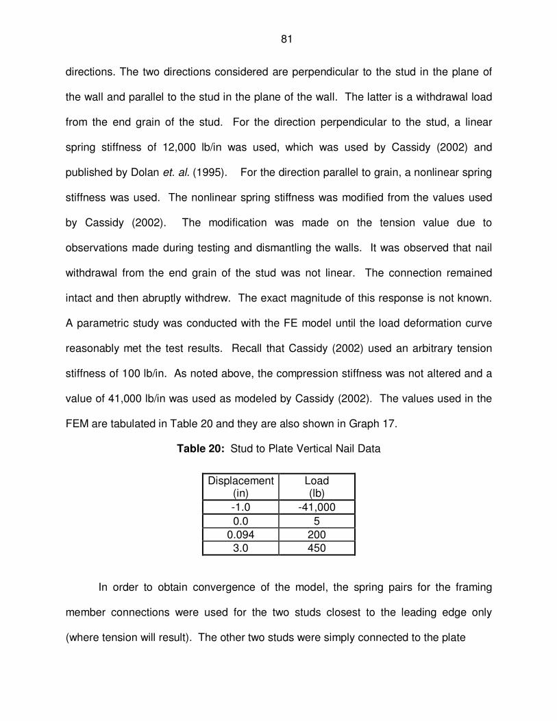
81
directions. The two directions considered are perpendicular to the stud in the plane of
the wall and parallel to the stud in the plane of the wall. The latter is a withdrawal load
from the end grain of the stud. For the direction perpendicular to the stud, a linear
spring stiffness of 12,000 lb/in was used, which was used by Cassidy (2002) and
published by Dolan et. al. (1995). For the direction parallel to grain, a nonlinear spring
stiffness was used. The nonlinear spring stiffness was modified from the values used
by Cassidy (2002). The modification was made on the tension value due to
observations made during testing and dismantling the walls. It was observed that nail
withdrawal from the end grain of the stud was not linear. The connection remained
intact and then abruptly withdrew. The exact magnitude of this response is not known.
A parametric study was conducted with the FE model until the load deformation curve
reasonably met the test results. Recall that Cassidy (2002) used an arbitrary tension
stiffness of 100 lb/in. As noted above, the compression stiffness was not altered and a
value of 41,000 lb/in was used as modeled by Cassidy (2002). The values used in the
FEM are tabulated in Table 20 and they are also shown in Graph 17.
Table 20: Stud to Plate Vertical Nail Data
Displacement (in)
Load (lb)
-1.0 -41,000
0.0 5
0.094 200 3.0 450
In order to obtain convergence of the model, the spring pairs for the framing
member connections were used for the two studs closest to the leading edge only
(where tension will result). The other two studs were simply connected to the plate

82
-1000
-800
-600
-400
-200
0
200
400
600
800
1000
-1.00 -0.50 0.00 0.50 1.00 1.50 2.00 2.50 3.00 3.50
Displacement, in
Lo
ad
, lb
Nail Data for Abaqus
Graph 17: 16d Stud Withdrawal Nail Data for ABAQUS
nodes. It was discovered that this is a good modeling technique to capture the behavior
of the framing connections.
It was recognized that the connection of the stud to the plate is neither an ideal
pinned connection nor a rigid connection. This joint is in fact a semi-rigid joint. When
the stud is in tension and the framing nails are withdrawing from the end grain of the
stud, the rotational stiffness of the joint is only the stiffness of the two 16d nails.
However, when there is a compression force in the stud, rigidity is created at the joint.
To illustrate the rigidity of the joint due to compression in the stud, a finite
element model was created, Figure 17, to observe the behavior of the joint. The model
consisted of a 2x4 member 6” tall. Since the base is supported on the sole or top plate,
compression only springs were used with the same stiffness as the compression
bearing shown in Table 20. RAM Elements was used for the FEA.
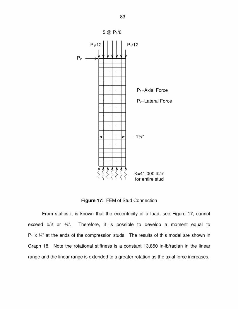
83
Figure 17: FEM of Stud Connection
From statics it is known that the eccentricity of a load, see Figure 17, cannot
exceed b/2 or ¾”. Therefore, it is possible to develop a moment equal to
P1 x ¾” at the ends of the compression studs. The results of this model are shown in
Graph 18. Note the rotational stiffness is a constant 13,850 in-lb/radian in the linear
range and the linear range is extended to a greater rotation as the axial force increases.
5 @ P1/6
P1/12 P1/12
K=41,000 lb/in for entire stud
P1=Axial Force
P2=Lateral Force
P2
1½”

84
Moment vs. Rotation
0
200
400
600
800
1000
1200
1400
0 0.02 0.04 0.06 0.08 0.1 0.12 0.14 0.16 0.18 0.2
Rotation, θθθθ (Radians)
Mo
men
t (i
n-l
b)
-1000
-2000
-3000
Axial Load, lb.
Graph 18: Effect of Axial Load on Stud Connection Rigidity
Figure 18 shows some of the results from the FEM with the 3,000 lb axial load
and a 100 lb lateral load. Figure 18 (a) shows the reactions, (b) shows the deformed
shape and (c) shows the axial stress.
(a)
(b)
(c)
Figure 18: FEM Results of Stud Connection Rigidity
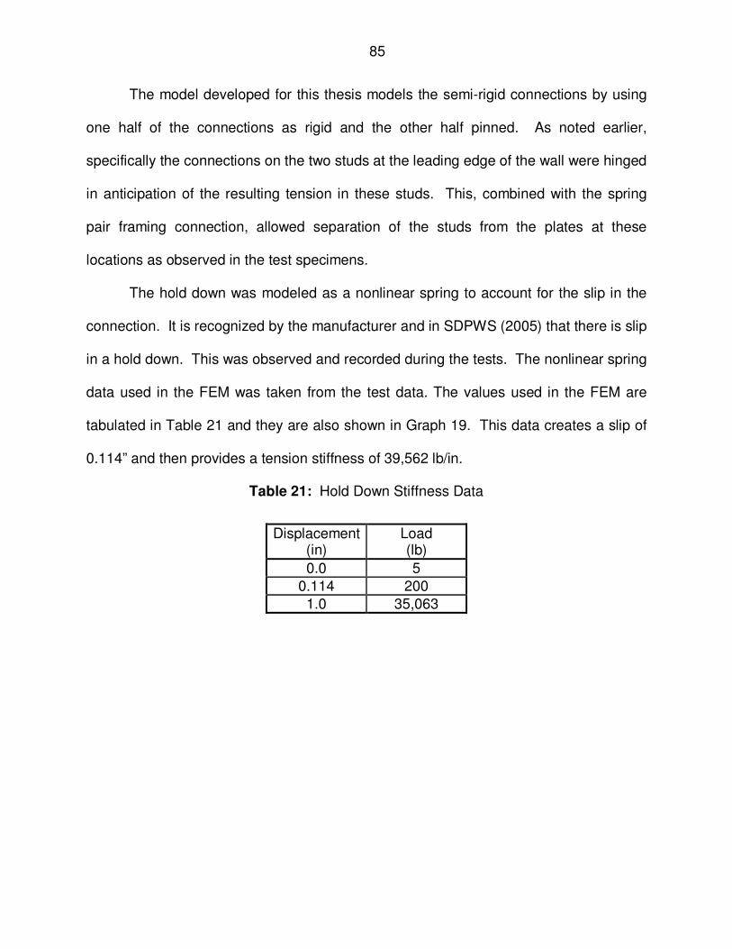
85
The model developed for this thesis models the semi-rigid connections by using
one half of the connections as rigid and the other half pinned. As noted earlier,
specifically the connections on the two studs at the leading edge of the wall were hinged
in anticipation of the resulting tension in these studs. This, combined with the spring
pair framing connection, allowed separation of the studs from the plates at these
locations as observed in the test specimens.
The hold down was modeled as a nonlinear spring to account for the slip in the
connection. It is recognized by the manufacturer and in SDPWS (2005) that there is slip
in a hold down. This was observed and recorded during the tests. The nonlinear spring
data used in the FEM was taken from the test data. The values used in the FEM are
tabulated in Table 21 and they are also shown in Graph 19. This data creates a slip of
0.114” and then provides a tension stiffness of 39,562 lb/in.
Table 21: Hold Down Stiffness Data
Displacement (in)
Load (lb)
0.0 5
0.114 200
1.0 35,063

86
0
500
1000
1500
2000
2500
3000
3500
4000
4500
5000
0 0.1 0.2 0.3
Displacement, in
Lo
ad
, lb
Hold Down Stiffness
Graph 19: Hold Down Stiffness for ABAQUS
4.3 Modeling
The FEM used displacement control in the load steps. Nonlinear geometry
control was used with the solver. The solver also used the Newton-Raphson method for
calculating the stiffness matrix. The ABAQUS line search control parameter was used
to help with convergence using the Newton-Raphson method.
The analysis utilized time steps to solve the model. The use of nonlinear
geometry required that a time step analysis was used. For convergence, the solver
automatically chose the step increment. An initial suggested step increment of 1/1000
was used with a maximum of 1/50. The solver was set to use smaller increments if
necessary. To further aid the convergence, a discontinuous analysis control was used.
This allows an increased number of iterations before divergence is checked. While this
can increase computational time, it was often necessary for convergence.

87
In addition to the constraining force, P, as shown in Figure 15, the dead load of
the wall was included in the analysis. This was applied as four 25 lb loads at the top of
the wall to account for the weight of the sheathing and framing members.
4.4 Finite Element Analysis Results
The model utilized the same boundary conditions and restraining force as the five
different sets tested, as well as one additional model with full constraint. The uplift
boundary constraints and restraining forces are summarized in Table 22. The additional
model with full constraint consisted of supports at 8” on center, along the top and
bottom. The supports along the top were connected to a rigid beam that was
constrained in both the vertical and out-of-plane directions. The supports directly above
and below the studs, as well as between the studs along the top plate, were no tension
elements. The supports between the studs along the bottom could resist tension. The
latter model is for illustration of a fully restrained wall. The results of all of the FE
models are shown on the following graphs and are each plotted along with the
corresponding test results.
Table 22: Summary of FE Model Constraints
Wall A B C D E Full
Constraint
Restraining Force, P (lb)
None 1104 2208 3312 None None1
Mechanical Hold Down
Y2 N3 N3 N3 N3 N4
1Rigid beam across top of wall preventing any uplift.
2Simulated mechanical hold down as used in actual tests.
3Simulated
5/8” diameter bolt 12” from tension edge.
4Simulated
5/8” diameter bolt at 8”, 24”, and 40” from tension edge.

88
Load Deformation Curve
0
100
200
300
400
500
600
-0.50 0.00 0.50 1.00 1.50 2.00 2.50 3.00 3.50 4.00 4.50 5.00 5.50
Displacement, inches
Lo
ad
, p
lf
Abaqus Model
Wall A1
Wall A2
Wall A3
Wall A4
Wall A5
Graph 20: FE Comparison for Wall A
Load Deformation Curve
0
50
100
150
200
250
300
350
400
-0.50 0.00 0.50 1.00 1.50 2.00 2.50 3.00 3.50 4.00 4.50
Displacement, inches
Lo
ad
, p
lf
Abaqus Model
Wall B-1
Wall B-2
Wall B-3
Wall B-4
Wall B-5
Graph 21: FE Comparison for Wall B
P
15/32” OSB
8d common 6:12 Spacing Mechanical Hold down
1104 lb
P
15/32” OSB
8d common 6:12 Spacing 5/8” AB

89
Load Deformation Curve
0
100
200
300
400
500
600
-0.50 0.00 0.50 1.00 1.50 2.00 2.50 3.00 3.50 4.00 4.50
Displacement, inches
Lo
ad
, p
lf
Abaqus Model
Wall C-1
Wall C-2
Wall C-3
Wall C-4
Wall C-5
Graph 22: FE Comparison for Wall C
Load Deformation Curve
0
100
200
300
400
500
600
700
-0.50 0.00 0.50 1.00 1.50 2.00 2.50 3.00 3.50 4.00 4.50 5.00
Displacement, inches
Lo
ad
, p
lf
Abaqus Model
Wall D-1
Wall D-2
Wall D-3
Wall D-4
Wall D-5
Graph 23: FE Comparison for Wall D
2208 lb
P
15/32” OSB
8d common 6:12 Spacing 5/8” AB
3312 lb
P
15/32” OSB
8d common 6:12 Spacing 5/8” AB
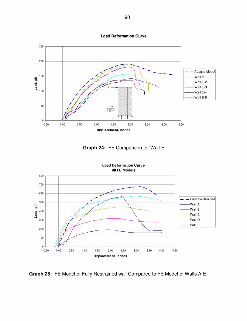
90
Load Deformation Curve
0
50
100
150
200
250
-0.50 0.00 0.50 1.00 1.50 2.00 2.50 3.00 3.50
Displacement, inches
Lo
ad
, p
lf
Abaqus Model
Wall E-1
Wall E-2
Wall E-3
Wall E-4
Wall E-5
Graph 24: FE Comparison for Wall E
Load Deformation Curve
All FE Models
0
100
200
300
400
500
600
700
800
-0.50 0.00 0.50 1.00 1.50 2.00 2.50 3.00 3.50 4.00 4.50
Displacement, inches
Lo
ad
, p
lf
Fully Constrained
Wall A
Wall B
Wall C
Wall D
Wall E
Graph 25: FE Model of Fully Restrained wall Compared to FE Model of Walls A-E
P
15/32” OSB 8d common 6:12 Spacing 5/8” AB
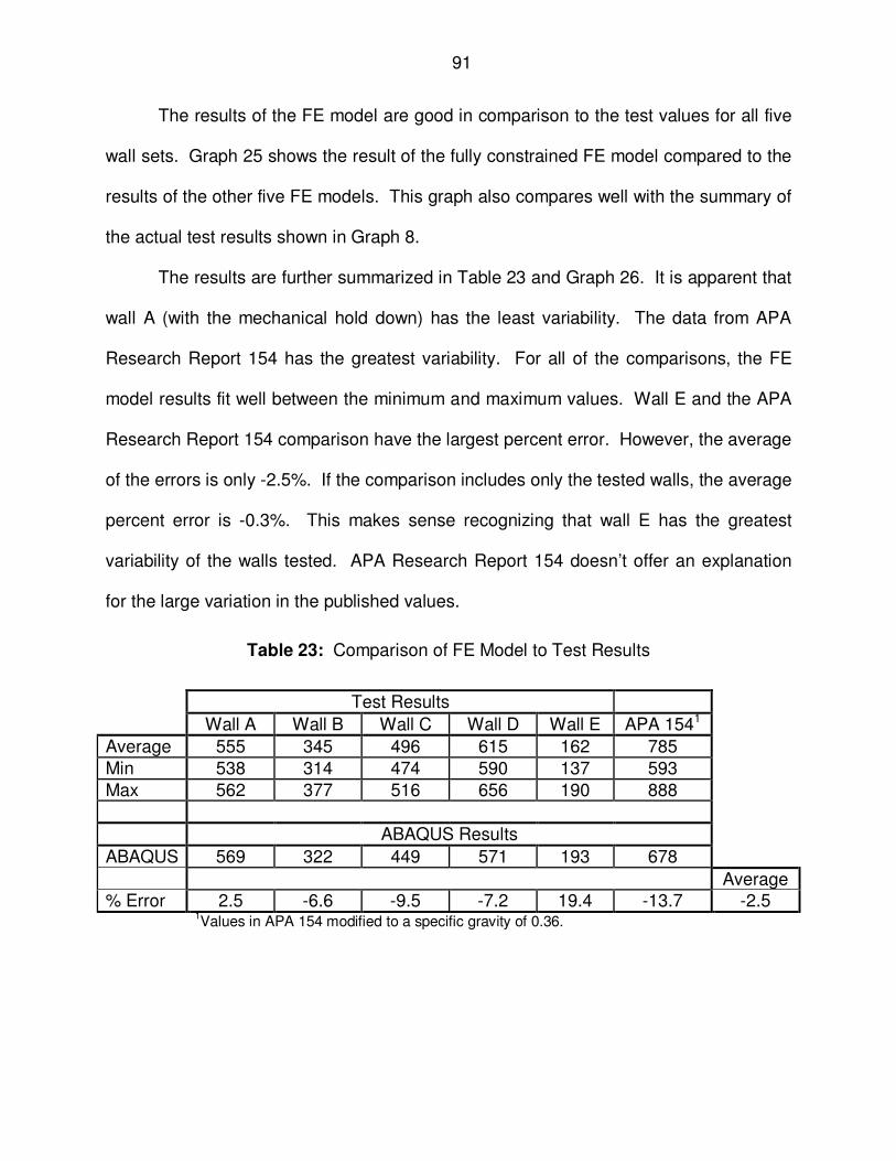
91
The results of the FE model are good in comparison to the test values for all five
wall sets. Graph 25 shows the result of the fully constrained FE model compared to the
results of the other five FE models. This graph also compares well with the summary of
the actual test results shown in Graph 8.
The results are further summarized in Table 23 and Graph 26. It is apparent that
wall A (with the mechanical hold down) has the least variability. The data from APA
Research Report 154 has the greatest variability. For all of the comparisons, the FE
model results fit well between the minimum and maximum values. Wall E and the APA
Research Report 154 comparison have the largest percent error. However, the average
of the errors is only -2.5%. If the comparison includes only the tested walls, the average
percent error is -0.3%. This makes sense recognizing that wall E has the greatest
variability of the walls tested. APA Research Report 154 doesn’t offer an explanation
for the large variation in the published values.
Table 23: Comparison of FE Model to Test Results
Test Results
Wall A Wall B Wall C Wall D Wall E APA 1541
Average 555 345 496 615 162 785
Min 538 314 474 590 137 593
Max 562 377 516 656 190 888
ABAQUS Results
ABAQUS 569 322 449 571 193 678
Average % Error 2.5 -6.6 -9.5 -7.2 19.4 -13.7 -2.5
1Values in APA 154 modified to a specific gravity of 0.36.

92
FE Comparison to Test Data
0
100
200
300
400
500
600
700
800
900
1000
Wall A Wall B Wall C Wall D Wall E APA 154
Wall Type
Lo
ad
, p
lf
Min
Average
Abaqus
Max
Graph 26: Comparison of FE Model to Test Results
Walls B, C and D have a negative movement initially due to the application of the
restraining force P. This was observed in the test walls as well. There is a P-∆ effect
that occurs when the restraining force, P, is applied since it is eccentric to the centroid
of the wall. There is also a prestess that occurs with an added restraining force, P. The
prestress, along with the added clamping action that keeps the plates from separating
from the studs, increases the unit shear capacity of the wall.
The partial restraint effect of a single anchor bolt 12” from the end of the wall is
best observed by viewing the sole plate as the wall is loaded. Figure 19 shows the
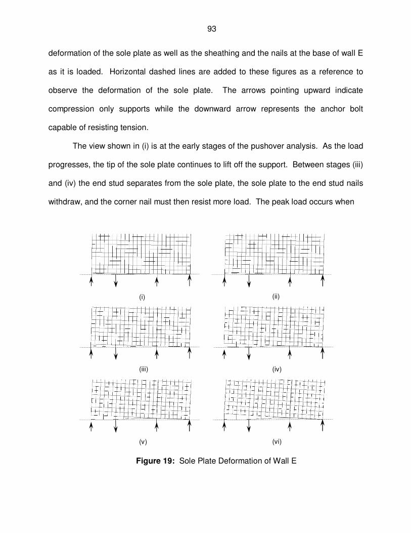
93
deformation of the sole plate as well as the sheathing and the nails at the base of wall E
as it is loaded. Horizontal dashed lines are added to these figures as a reference to
observe the deformation of the sole plate. The arrows pointing upward indicate
compression only supports while the downward arrow represents the anchor bolt
capable of resisting tension.
The view shown in (i) is at the early stages of the pushover analysis. As the load
progresses, the tip of the sole plate continues to lift off the support. Between stages (iii)
and (iv) the end stud separates from the sole plate, the sole plate to the end stud nails
withdraw, and the corner nail must then resist more load. The peak load occurs when
(i)
(ii)
(iii)
(iv)
(v)
(vi)
Figure 19: Sole Plate Deformation of Wall E
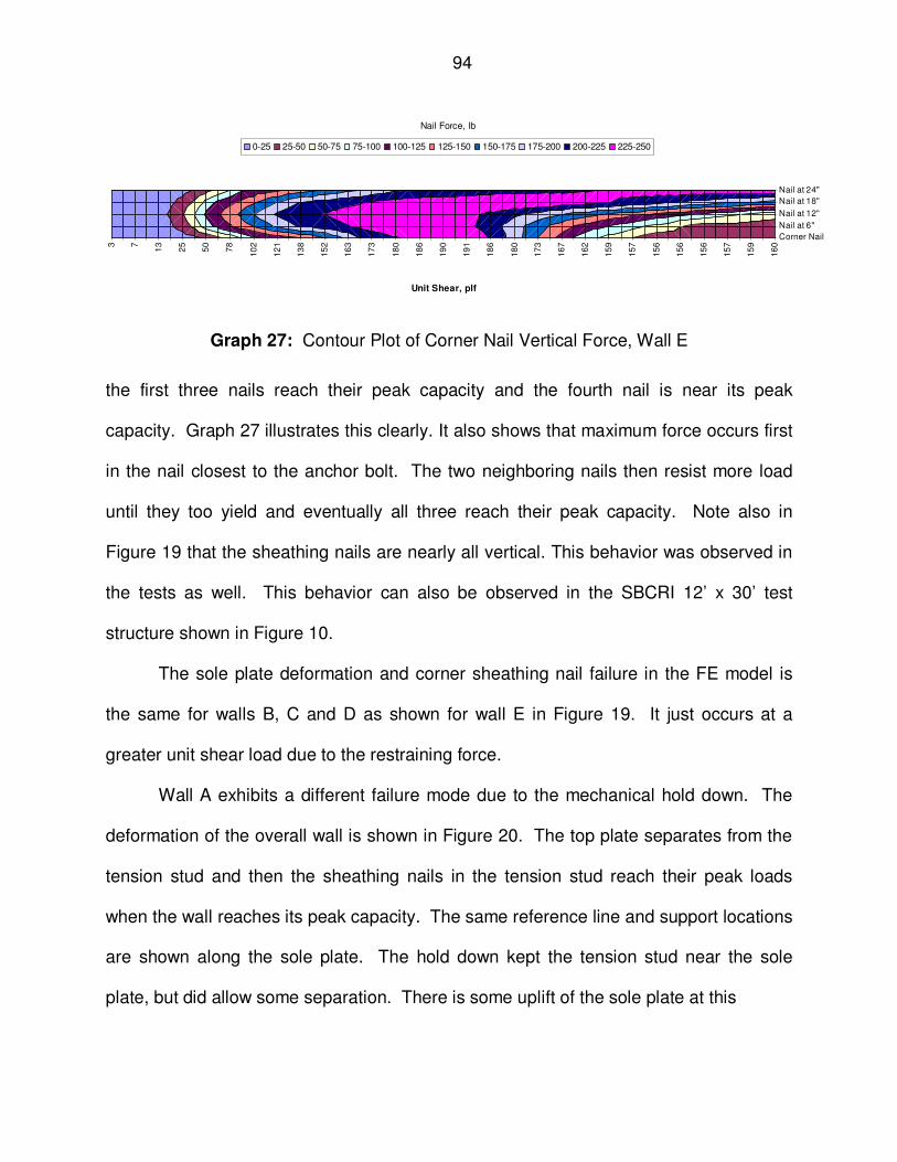
94
3 7
13
25
50
78
10
2
12
1
13
8
15
2
16
3
17
3
18
0
18
6
19
0
19
1
18
6
18
0
17
3
16
7
16
2
15
9
15
7
15
6
15
6
15
6
15
7
15
9
16
0
Corner Nail
Nail at 6"
Nail at 12"
Nail at 18"
Nail at 24"
Unit Shear, plf
0-25 25-50 50-75 75-100 100-125 125-150 150-175 175-200 200-225 225-250
Nail Force, lb
Graph 27: Contour Plot of Corner Nail Vertical Force, Wall E
the first three nails reach their peak capacity and the fourth nail is near its peak
capacity. Graph 27 illustrates this clearly. It also shows that maximum force occurs first
in the nail closest to the anchor bolt. The two neighboring nails then resist more load
until they too yield and eventually all three reach their peak capacity. Note also in
Figure 19 that the sheathing nails are nearly all vertical. This behavior was observed in
the tests as well. This behavior can also be observed in the SBCRI 12’ x 30’ test
structure shown in Figure 10.
The sole plate deformation and corner sheathing nail failure in the FE model is
the same for walls B, C and D as shown for wall E in Figure 19. It just occurs at a
greater unit shear load due to the restraining force.
Wall A exhibits a different failure mode due to the mechanical hold down. The
deformation of the overall wall is shown in Figure 20. The top plate separates from the
tension stud and then the sheathing nails in the tension stud reach their peak loads
when the wall reaches its peak capacity. The same reference line and support locations
are shown along the sole plate. The hold down kept the tension stud near the sole
plate, but did allow some separation. There is some uplift of the sole plate at this

95
Figure 20: Deformation of Wall A FE Model
point due to slip and elongation of the hold down. This behavior was observed in the
tests as well.
The fully restrained FE model illustrates the behavior of the wall when the plates
are not allowed to separate from the studs. This can occur if a test apparatus utilizes a
stiff load beam bolted to the top, if anchor bolts are used in each stud space, and if hold
down rods are used to anchor the load beam to the foundation as illustrated in ASTM
E72, Figure 22.
Separation of top plate
from end stud
Hold down restraining
corner of wall
Enlargement of hold down response

96
For the fully restrained FE model,
the peak load was reached when the
peak capacity of the nails in the
compression stud was reached. The
deformation of the studs can be seen in
Figure 21. At peak load the studs
transferred 869 lb of shear at the top
plate and 894 lb of shear at the sole
plate. This is an average force of 220 lb
per stud connection or 220 plf of
additional unit shear capacity beyond
the sheathing edge nail contribution.
This can add a significant increase to the wall unit shear capacity when the wall is fully
restrained. This also explains the difference in the nail load deformation curves shown
in Graph 9.
The contributing effect of the wall studs to the unit shear capacity was also
observed in the other wall models, but to a lesser degree. The full benefit of the stud
resistance cannot be achieved without a full constraint condition or other mechanical
means of keeping the studs from separating from the plates.
The sheathing is not shown in Figure 21 for clarity to show the framing
deformation. The rigid beam along the top of the wall is also shown in Figure 21.
Figure 21: Deformation of Fully Restrained FE Model Frame

97
CHAPTER 5
RELIABILITY ANALYSIS
The calibration using a reliability analysis was conducted in stages to fully
understand the effect of each random variable and load combinations. It was necessary
to first determine the reliability of the current industry standard, SDPWS, so a target
reliability index could be used to determine the correct bias factors to produce the
proper nominal values. The end result is verification of the nominal unit shear value
used in SDPWS along with modifications for specific gravity, and proposed modification
factors for the restraint type and partial restraining force; all of which are calibrated to
the target reliability index.
At the two extremes of a partially restrained shear wall are unrestrained and fully
restrained. The unrestrained shear wall is not restrained by any special mechanical
hold down device or restraining force. The unrestrained shear wall is only restrained by
the ½” diameter anchor bolt 12” from the end as required by the IRC. The fully
restrained shear wall is restrained completely by an applied restraining force at the top
of the wall. This load is so large that it produces a righting moment such that the
overturning force will never overcome it. The failure modes of these two shear wall
conditions have nothing to do with the variability of the restraining force and thus are
only dependent upon their unit shear strength and the specific gravity of the lumber.
The load combinations of ASCE 7 and the IBC will have an effect on the
partially restrained conditions between the two extremes explained in the preceding

98
paragraph. The calibration stage process presented will clearly illustrate the effect of
these load combinations.
5.1 Code Required Load Combinations
Both ASCE 7-05 and IBC 2009 provide requirements for load combinations that a
structure must meet. SDPWS provides the required ASD safety factor and LRFD
resistance factor, (section 2.6). The governing load combinations for wood shear walls
with wind load, the corresponding ASD safety factor and LRFD resistance factor are
summarized in Table 24.
Table 24: Load Combinations
ASD LRFD
Load Combination Safety Factor, Ω1 Load Combination Resistance Factor, φ1 D+W 2.0 1.2D+1.6W 0.8
0.6D+W 2.0 0.9D+1.6W 0.8 1 From SDPWS
D=Dead Load W=Wind Load
5.2 Reliability of SDPWS Nominal Unit Shear Capacities
It is necessary to understand the reliability of the current unit shear capacities in
order to calibrate the partially restrained shear wall unit shear capacities. To
accomplish this, the origination of the SDPWS values was researched. The values in
SDPWS originate from APA Research Report 154.
The test results, shown in Table 12, indicate that a mechanical hold down device
at the bottom tension corner is not sufficient to achieve the fully restrained shear wall
capacity. Therefore, to determine the capacity of a fully restrained shear wall, the
values published in APA Report 154 were used and are indicated here for the 15/32”

99
WSP as used for the test samples. The nominal design unit shear capacity for 15/32”
WSP are based on the results of seven tests, Table 25. The seven test results are a
combination of three tests using 19/32” plywood and four tests using 5/8” plywood. The
panel thickness has little influence on the ultimate capacity of the shear wall (van de
Lindt and Rosowsky 2005). Therefore, it is reasonable to use the test results shown in
Table 26 as the ultimate unit shear capacity for 15/32” WSP.
Table 25: Excerpt from APA Report 154, Table A1
Fastener Ultimate Loads (plf)
Size Spacing
(in)
Panel Thickness(a)
(in)
No. of Tests Min. Max. Avg.
Target Design Shear
Load Factor(b)
RATED SHEATHING 8d 6 15/32 7 689 1033 913 260 3.5
(a) Minimum panel thickness for design shear, some walls sheathed with thicker panels. (b) The load factor is determined by dividing the average ultimate load by the target design shear.
A summary of the reported test results shown in Table 25 and Table 26 are
shown in Table 27. Since all four tests are not reported for the 5/8” WSP, the two missing
values were estimated with equal weight.
Table 26: Excerpt from APA Report 154, Table A2
Fastener Panel Ultimate Loads
(plf)
Size Spacing
(in) Type Thickness
(in)
No. of
Tests Min. Max. Avg.
Target Design Shear
Load Factor(a)
RATED SHEATHING 19/32 3 950 1033 992 260(b) 3.8 8d 6 Plywood 5/8 4 689 1000 854 260(b) 3.3
(a) The load factor is determined by dividing the average ultimate load by the target design shear. (b) Design shear increased for “over-thick” panel, studs 16” o.c. or panel placed with 8’ length
perpendicular to framing.

100
Table 27: Summary of APA Report 154
950992
1033689
1000863.5 1
863.5 1
Average 913Standard Deviation 119COV 0.131Estimated from data in APA Report 154.
Ultimate Capacity
(plf)
19/32
Panel Thickness (in)
5/8
The standard deviation and distribution of the APA wall tests are needed to
calculate the reliability of SDPWS. Table 27 includes one of these two parameters.
The distribution is expected to be lognormal as found with the test results reported in
Section 3.3.4. To verify the accuracy of the COV in Table 27, it was compared with the
5% lower exclusion value for the data from APA Report 154. Table 28 shows that the
calculated standard deviation is very close to the 5% lower exclusion value. Since the
5% lower exclusion value is commonly used for timber design values, the actual
standard deviation of ultimate unit shear capacity from the APA test data is more
accurately 112 plf.
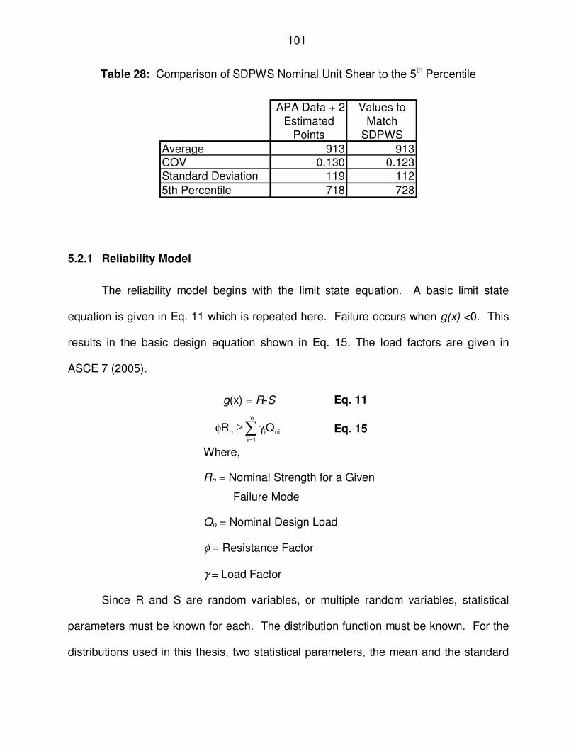
101
Table 28: Comparison of SDPWS Nominal Unit Shear to the 5th Percentile
Average 913 913COV 0.130 0.123Standard Deviation 119 112
5th Percentile 718 728
APA Data + 2 Estimated
Points
Values to Match
SDPWS
5.2.1 Reliability Model
The reliability model begins with the limit state equation. A basic limit state
equation is given in Eq. 11 which is repeated here. Failure occurs when g(x) <0. This
results in the basic design equation shown in Eq. 15. The load factors are given in
ASCE 7 (2005).
g(x) = R-S Eq. 11
Eq. 15
Where,
Rn = Nominal Strength for a Given
Failure Mode
Qn = Nominal Design Load
φ = Resistance Factor
γ = Load Factor
Since R and S are random variables, or multiple random variables, statistical
parameters must be known for each. The distribution function must be known. For the
distributions used in this thesis, two statistical parameters, the mean and the standard
∑=
γ≥φm
1iniin QR

102
deviation, are needed. Additionally the random variables must be identified. The wind
load, the shear wall strength, the dead load restraining force, and the specific gravity of
the framing lumber have been identified as random variables. Of these four random
variables, the parameters are known for wind load (van de Lindt and Rosowsky 2005),
the dead load (Ellingwood, et al 1980), and the specific gravity (ASTM D2555). The
parameters for the shear wall unit shear strength were determined from the wall testing
presented in this thesis. Table 29 summarizes the parameters known thus far.
Table 29: Summary of Distributions
Item nXX
vx (cov) DF Dead Load 1.05 0.1 Normal
Wind Load 0.8 0.35 Type 1 Specific Gravity, G 1.0 0.11 Lognormal2
Shear Wall Capacity Unknown Varies3 Lognormal3 1From ASTM D 2555 2From specific gravity test of lumber from samples
3From shear wall test results
The formation of the limit state function, g(x), then includes the unit shear
strength of the shear wall, V, the specific gravity of the framing lumber, G, the wind load,
VW, and the dead load, P. For the limit state of shear:

103
Eq. 16
Eq. 17
Eq. 18
Eq. 18 shows the relationship of the average shear load to the bias factor,
resistance factor, load factor, and the nominal unit shear strength.
5.2.2 Reliability Analysis Results
Since the SDPWS shear wall is considered as fully restrained, only two of the
four random variables are considered to determine the reliability of the SDPWS unit
shear capacity. The two random variables are the wall shear strength and the wind
load. These two random variables were applied to Eq. 11. Using the first order second
moment, FOSM, reliability method the reliability index β was determined to be 3.27 for
the 15/32” shear wall tabulated in SDPWS for a fully restrained condition. Recall from
Section 2.6 that the SDPWS values are 2.8 times the APA Report 154 target design
shear. Therefore, as determined by the quotient of the average ultimate load, 913 plf, in
)).(( G501VV tabn −−=
un VV ≥φ
nWWu VVV φ=γ=
W
nW
VV
γ
φ=
W
n1W1W
VaVaV
γ
φ==
load shear V
windto due load shear UnfactoredV
factor bias load a
gravitySpecific
values shear unit SDPWS
Where,
W
W
1
Average
Wind
G
Vtab
=
=
=
=
=

104
Table 25 and the nominal unit shear capacity, 730 plf, in SDPWS, Table 6, the bias
factor used in SDPWS is 1.25. The calculations are shown in Appendix D.
The target reliability index, β, for the calibration of the partially restrained shear
walls tested will be 3.25 since the SDPWS nominal unit shear capacity has a reliability
index of 3.27. This is reasonable based on other literature (van de Lindt and Rosowsky
2005).
5.3 Base Calibration of Partially Restrained Unit Shear Capacities
The reliability index of the unit shear capacity of the unrestrained shear wall was
calculated next. Using the mean unit shear capacity of wall E, 162 plf, from Table 12,
the reliability index was calculated using the FOSM method. The calculations are
shown in Appendix E for a bias factor of 1. With a bias factor of 1, the reliability index,
β, was determined to be 2.59, Table 30. The calculations were iterated changing the
bias factor, Table 30, and the results were plotted in Graph 28. The calibrated bias
factor was determined from the graph and verified again with calculation. A summary of
the results is shown in Table 30.
This procedure was repeated for the remaining partially restrained walls A, B, C,
and D. A summary of the results are shown in Table 31. Note that the calibrated
values shown in Table 31 simply calibrate all of the partial restraint conditions from the
tests and the SDPWS (APA) values to the target reliability index, β=3.25. This is
appropriate for the ASD load combination D+W with a safety factor, Ω=2.0. For the
mechanical hold down, Group A walls, the unrestrained Group E walls, and the SDPWS

105
(APA) fully restrained wall, this is also appropriate for the LRFD load combination
1.2D+1.6W with a resistance factor, φ=0.8.
Table 30: Nominal Unit Shear Calibration for Unrestrained Wall E
V(Strength) Vw(Load)
uVN aV uV σV uVwN aVw uVw σVw
plf plf Plf plf plf plf
β
162.0 1.00 162 23.5 81.0 0.8 64.8 22.7 2.59
154.3 1.05 162 23.5 77.1 0.8 61.7 21.6 2.72
147.3 1.10 162 23.5 73.6 0.8 58.9 20.6 2.84
140.9 1.15 162 23.5 70.4 0.8 56.3 19.7 2.96
135.0 1.20 162 23.5 67.5 0.8 54.0 18.9 3.07
129.6 1.25 162 23.5 64.8 0.8 51.8 18.1 3.19
126.6 1.28 162 23.5 63.3 0.8 50.6 17.7 3.25
124.6 1.30 162 23.5 62.3 0.8 49.8 17.4 3.3
120.0 1.35 162 23.5 60.0 0.8 48.0 16.8 3.39
115.7 1.40 162 23.5 57.9 0.8 46.3 16.2 3.49
111.7 1.45 162 23.5 55.9 0.8 44.7 15.6 3.59
108.0 1.50 162 23.5 54.0 0.8 43.2 15.1 3.69
104.5 1.55 162 23.5 52.3 0.8 41.8 14.6 3.78
The reason that the nominal unit shear values shown in Table 31 are appropriate
for the ASD and LRFD load combinations stated is that the dead load will not affect the
wall strength in these load combinations. There are additional load combinations (Table
24) which require a reduced load factor for the dead load. This insures that dead load
will not be a limiting factor and these combinations are addressed in section 5.4.
Therefore, the unit shear capacity of the wall is the only random variable on the strength
side considered for this step.
To illustrate the relationship between partial restraint and nominal unit shear
strength, the results shown in Table 31 are graphed in Graph 29. Note that the shape
of the graph is similar to Graph 12. The difference between these two graphs is shown
in Graph 30. Note that the fully restrained wall has 100% unit shear capacity in both the

106
0
20
40
60
80
100
120
140
160
180
2.5 2.75 3 3.25 3.5 3.75 4 4.25 4.5
No
min
al U
nit
Sh
ear
Str
en
gth
, p
lf
Reliability Index, ββββ
Wall E - Unrestrained
Graph 28: Calibration of Unrestrained Shear Wall
nominal, calibrated, the ultimate and test result. They are the same due to the
normalization. The unrestrained wall is nearly the same as well. The larger difference
occurs for walls B, C, and D. This difference is due to the shift in the percent of full
restraint. The mechanical hold down cannot achieve the same unit shear capacity as a
wall restrained from the top. This was discussed in Section 3.3.3. The difference in the
two points in Graph 30 is from the calibration as well as the percent of full restraint
occurring in the normalization process.

107
Table 31: Calibrated Shear Wall Capacities
Calibrated Wall Values1
A B C D E SDPWS2 Wall Restraint
(lb) 4416 1104 2208 3312 0 5051
Ultimate Unit Shear Capacity (from tests), plf
555 345 496 615 162 786
Bias Factor
a2 1.15 1.19 1.16 1.16 1.28 1.25
Nominal Unit Shear Capacity, plf
483 289 428 529 127 631
Normalized
Phold down 0.874 0.219 0.437 0.656 0.000 1
Vcap(%) 0.764 0.458 0.678 0.838 0.200 1.000 1Calibrated for ASD load combination D+W
2From SDPWS and APA Report 154
a2 = Unit shear capacity bias factor
y = 0.797x + 0.2664R² = 0.962
y = -0.5088x2 + 1.3094x + 0.1993R² = 0.9999
0%
20%
40%
60%
80%
100%
120%
0% 20% 40% 60% 80% 100% 120%
% o
f F
ull
Sh
ea
r C
ap
ac
ity
% of Full Restraining Force
Test Data + APA
Holdown
Linear (Test Data + APA)
Poly. (Test Data + APA)
Linear Fit
Second Order Fit
Graph 29: Partial Restraint Effect on Strength - Calibrated
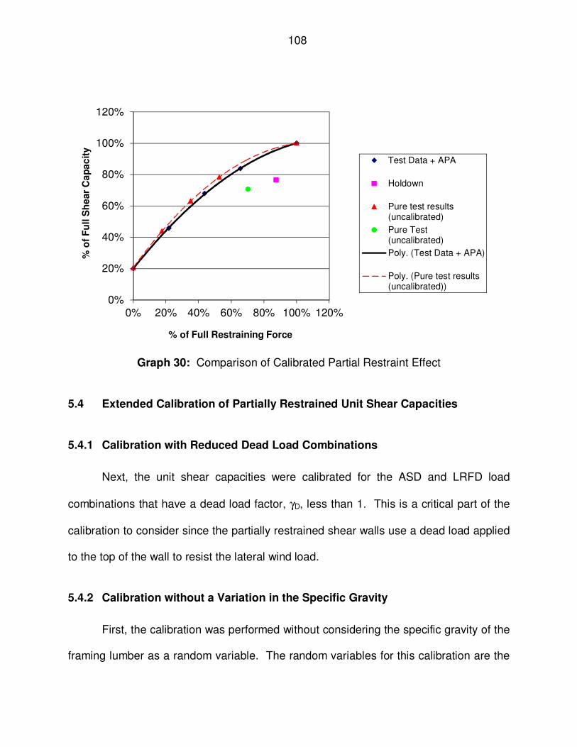
108
0%
20%
40%
60%
80%
100%
120%
0% 20% 40% 60% 80% 100% 120%
% o
f F
ull S
he
ar
Ca
pa
cit
y
% of Full Restraining Force
Test Data + APA
Holdown
Pure test results(uncalibrated)
Pure Test(uncalibrated)
Poly. (Test Data + APA)
Poly. (Pure test results(uncalibrated))
Graph 30: Comparison of Calibrated Partial Restraint Effect
5.4 Extended Calibration of Partially Restrained Unit Shear Capacities
5.4.1 Calibration with Reduced Dead Load Combinations
Next, the unit shear capacities were calibrated for the ASD and LRFD load
combinations that have a dead load factor, γD, less than 1. This is a critical part of the
calibration to consider since the partially restrained shear walls use a dead load applied
to the top of the wall to resist the lateral wind load.
5.4.2 Calibration without a Variation in the Specific Gravity
First, the calibration was performed without considering the specific gravity of the
framing lumber as a random variable. The random variables for this calibration are the

109
unit shear capacity, V, the wind load, VW, and the dead load, P. These random
variables are defined in Table 29.
The shear wall ultimate unit shear capacity is a function of the restraining force.
As shown in Eq. 14, the ultimate unit shear capacity of a partially restrained shear wall
is related to the fully restrained shear wall unit shear capacity by the partial restraint
factor, Cpr-u. This relationship was used for the second calibration. Since the restraining
force, PD, is a random variable, then Cpr-u varies. However, Cpr-u cannot be greater than
1. This limit cannot be accounted for in a FOSM model. Therefore, for the second
calibration, a Monte Carlo simulation was used.
The Monte Carlo simulation was conducted in Excel 2010. To adequately capture
the target reliability index, β, of 3.25 (pf = 5.77e-4), four million simulations were used.
This was done by repeating 100,000 simulations 40 times for each increment of bias
factor studied. The calibration consisted of varying the bias factor to achieve the target
reliability index, β=3.25; similar to what was done with the first calibration with the test
data. The results were graphed to determine the calibrated bias factor similar to Graph
28. The value from the graph was then confirmed with 4 million simulations. The Monte
Carlo simulation is described below.
5.4.3 Random Variables used for Calibration
The nominal shear capacity of the wall is:

110
or,
Since V is a random variable, Vn is a random variable as well. For this step, the
specific gravity, G, is considered a constant.
Recall from Eq. 14 that the partially restrained unit shear capacity is the fully
restrained unit shear capacity modified by the partial restraint factor (Eq. 13) which is
repeated here:
Cpr-u = -0.6393λ2+1.4331λ+0.206 ≤ 1.0 Eq. 13
height wallshearh
capacity shear unit ultimate averageV
variable) (random force grestraininP
hV
P
ult
D
ult
D
=
=
=
×=λ
Therefore,
Eq. 19
2
n
aV
V=
factor biasCapacity Sheara
Where,
2 =
2
na
VV =
( )( )
2
na
G501VV
−−=
.
( )( )
2
upr
na
G501VCV
−−=
− .

111
The mean dead load restraining force applied to the wall is:
Adding the load factor:
Eq. 20
The nominal wind load is taken as the nominal capacity of the shear wall.
Therefore, the nominal wind load is calculated as shown here:
Eq. 21
or,
Eq. 22
3
n
Da
P
P=
factor load Dead
factor bias load Deada
Where,
D
3
=γ
=
D3D PaP =
D
D3D
PaP
γ=
W
nnW
VV
γ
φ=
nWW VaV 1=
W
n1W
VaV
γ
φ=
factor load Wind
factor resistance
factor bias load Winda
variable) (random shear unit load windmeanV
variable) (random shear unit load windminalnoV
Where,
W
1
W
Wn
=γ
=φ
=
=
=

112
And, for a partially restrained shear wall, the limit state equation is:
Eq. 23
5.4.4 Random Variable Distributions
Although Eq. 23 only indicates two random variables, keep in mind that there is a
third random variable, PD, included in the partial restraint factor, Cpr-u. Table 34
summarizes the three random variables necessary for Eq. 23 and the Monte Carlo
simulation. The bias factor for V is indicated as “unknown” because this is what is being
determined by the calibration.
Table 32: Summary of Distributions
Random Variable Item nX
X vx (cov) DF
PD Dead Load 1.05 0.1 Normal
VW Wind Load 0.8 0.35 Type 1
V Shear Wall Capacity
Unknown 0.123 Lognormal4
1From ASTM D 2555 2From specific gravity test of lumber from samples 3From Table 28 4From shear wall test results
5.4.5 Steps used for Monte Carlo Simulation
The Monte Carlo simulation was conducted with the following steps:
1. Begin with the restraining force. This is the restraining force from walls B, C, and
D; 1104 lb, 2208 lb, and 3312 lb respectfully.
a. Calculate the mean dead load restraining force, DP , using Eq. 20 and its
bias factor shown in Table 32.
( ) WW VVVVg −=,
wallthe ofcapacity shear unit V
shear unit load windV
Where,
W
=
=

113
2. Calculate the partial restraining factor, Cpr-u, Eq. 13 using the restraining force
from step 1.
3. Determine the mean ultimate unit shear strength, V , from APA Report 154, and
its statistical properties.
4. Start with a trial bias factor, a2=0.8.
5. Calculate the nominal unit shear strength, Vn, using Eq. 19, with the specific
gravity of the wall framing members, G=0.36 for SPF –S.
6. Calculate the nominal wind load, VWn, using Eq. 21.
7. Calculate the mean wind load, WV , using Eq. 22 and its statistical properties.
8. Monte Carlo Simulation
a. Use a random number generator to generate a random probability
between 0 and 1 and calculate the inverse of the CDF (normal distribution)
for the dead load, PD, at the random probability.
b. Using the result of step 8.a, calculate Cpr-u using Eq. 13.
c. Use a random number generator to generate a random probability
between 0 and 1 and calculate the inverse of the CDF (lognormal
distribution) for the unit shear capacity, V, at the random probability.
d. Calculate the partially restrained unit shear capacity of the wall by
modifying the unit shear capacity, V, from step 8.c by the partial restraint
factor, Cpr-u, from step 8.b.
e. Use a random number generator to generate a random probability
between 0 and 1 and calculate the inverse of the CDF (Type I extreme
value distribution) for the wind load, VW, at the random probability.
f. Using Eq. 23 calculate the survival of the function (g(x)>0 for survival).
Set a flag equal to zero for survival or one for failure.
g. Repeat steps 8.a to 8.f 100,000 times, and add the number of failures in
step 8.f.
9. Repeat step 8 forty times and sum the total number of failures from step 8.g.
Calculate the reliability of the 4,000,000 samples and then calculate the reliability
index, β as shown:

114
)R(
R
pR f
−Φ=β
−=
−=
− 1
4,000,000
failures of #1
1
1
10. Plot the bias factor, a2, and the reliability index, β, from step 9.
11. Increase the bias factor, a2, increment (0.1 was used) and repeat steps 5 to 11
until 253.≥β .
12. Using the graph from step 10, determine the correct bias factor, a2, to obtain the
target reliability index β=3.25.
13. Repeat steps 5 to 9 to validate the bias factor, a2, determined in step 12.
14. Make correction to the bias factor a2 if necessary and repeat steps 5 to 9.
15. Repeat entire procedure for next wall set (restraining load).
An illustration of the Excel spreadsheet used for the Monte Carlo simulation is
shown in Appendix F.
5.4.6 Calculations for Monte Carlo Simulation
The known distributions of each random variable were used in the MCS to
generate random values to evaluate Eq. 11. As shown in Table 32 and again in Table
34, three distributions were used, Normal, Log-Normal, and Type I. The cumulative
distribution function, CDF, for each of these was used along with a random number
generator to generate values of the random variables. The random number generator is
used to generate a probability which can then be evaluated with the CDF to determine
the random variable value at the generated probability.
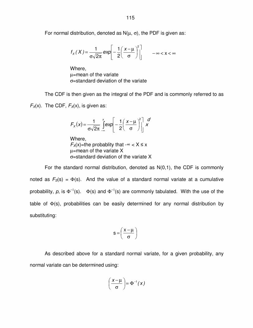
115
For normal distribution, denoted as N(µ, σ), the PDF is given as:
Where, µ=mean of the variate σ=standard deviation of the variate
The CDF is then given as the integral of the PDF and is commonly referred to as
FX(x). The CDF, FX(x), is given as:
Where, FX(x)=the probablity that -∞ < X ≤ x µ=mean of the variate X σ=standard deviation of the variate X
For the standard normal distribution, denoted as N(0,1), the CDF is commonly
noted as FS(s) = Φ(s). And the value of a standard normal variate at a cumulative
probability, p, is Φ−1(s). Φ(s) and Φ−1(s) are commonly tabulated. With the use of the
table of Φ(s), probabilities can be easily determined for any normal distribution by
substituting:
As described above for a standard normal variate, for a given probability, any
normal variate can be determined using:
σ
µ−−
πσ=
2
2
1
2
1 xexp)X(fX ∞<<∞− x
( ) dx∫
∞−
σ
µ−−
πσ=
x
X
xexpxF
2
2
1
2
1
σ
µ−=
xs
)x(x 1−Φ=
σ
µ−

116
Therefore, for any given probability, Φ(x), the value of x can by calculated. A
random number generator is used to generate the probability Φ(x) for which a given
value for the random variate X is calculated using Φ-1 (x). Therefore, if p is a random
probability, Φ(x), the value of the random variate is calculated as:
Where, p= probability that -∞ < X ≤ x, and is randomly generated µ=mean of the variate X σ=standard deviation of the variate X
The use of this for the MCS is illustrated in Appendix F.
For lognormal distribution, the PDF is given as:
Where,
The parameters λ and ζ are related to the mean µ and the standard deviation σ
of the variate as (Ang and Tang, 1975):
ζ
λ−−
ζπσ=
2
X
x
2
1
x2
1xf
lnexp)( ∞<≤ x 0
)(ln
)(ln
XVar
XE
=ζ
=λ
µ
σ+=ζ
ζ−µ=λ
2
22
2
1
2
1
ln
ln
µ+σ=
=Φ
Φ=
=≤<−∞
−
sx
on,distributi normal standard
the for tabulated is CDF the Since
1 x)p(
)x(p
p)xX(P

117
If σ/µ is ≤ 0.30, then,
The CDF is then given as the integral of the PDF and is given as:
Where, P=the probability that X is between a and b λ=mean of the lognormal of the variate X ζ=standard deviation of the lognormal of the variate X
The lognormal distribution of a random variable X is a normal distribution of the
natural logarithm of X. Therefore, the commonly tabulated values of Φ(s) and Φ−1(s) for
standard normal distribution can be used similarly to the description earlier where:
And also similar to the explanation above for normal distribution, for a given
probability, the normal variate can be determined using:
Therefore, for any given probability, Φ(x), the value of x can by calculated. A
random number generator is used to generate the probability Φ(x) for which a given
value for the random variate X is calculated using Φ-1 (x). Therefore, if p is a random
probability, Φ(x), the value of the random variate is calculated as:
µ
σ≈ζ
dx∫
ζ
λ−−
ζπσ=≤<
b
a
2x
2
1
x2
1bXaP
lnexp)(
ζ
λ−=
xs
ln
)x(xln 1−Φ=
ζ
λ−

118
Where, p= probability that -∞ < X ≤ x, and is randomly generated λ=mean of the lognormal of the variate X ζ=standard deviation of the lognormal of the variate X
The use of this for the MCS is illustrated in Appendix F.
For the Gumbel Type I distribution, the CDF is given as Eq. 9 and is repeated
here:
( ) ( )( )[ ] ∞<<∞−−α−−= xuxexpexpxF nXn Eq. 9
Where, un = location parameter αn = scale parameter
The location and scale parameters are related to the mean and standard
deviation of the random variable X as:
n
xn
x
n
u
6
α
γ−µ=
σ
π=α
Where,
αn = scale parameter un = location parameter σx = standard deviation of random variable X
µx = mean of random variable X γ = Euler’s Constant = 0.577216
( )λ+ζΦ=
=Φ
Φ=
=≤<−∞
−
−
)x(exp
x)p(
)x(p
p)xX(P
1
1
x
on,distributi normal standard
the for tabulated is CDF the Since

119
Since the CDF is given directly in Eq. 9, the probability that -∞ < X ≤ x is FXn(x).
Eq. 9 can be rearranged, Eq. 24, to solve for the value of x at a random probability:
( )( )[ ] 1xFlnlnux
nX
n
n −α
−= Eq. 24
Where, un = location parameter αn = scale parameter FXn
(x) = probability of Xn, and is randomly generated
The use of this for the MCS is illustrated in Appendix F.
5.4.7 Results of the Monte Carlo Simulation for ASD
The results of the MCS for the ASD load combination 0.6D+W are summarized in
Table 33 for wall Groups A, B, C, D, E, and SDPWS. The values for A, E, and SDPWS
are from the FOSM analysis summarized in Table 31. For these walls, the restraining
force was not the limit state of failure and was not modeled in the MCS. The ASD load
combination will assure there is enough dead load for these conditions.
Table 33 summarizes the restraining force, the average unit shear capacity from
the test results and SDPWS, the bias factor from the calibration, and the resulting
nominal unit shear capacity. The nominal unit shear capacity was then normalized to
the SDPWS nominal unit shear capacity. Similarly, the ratio of the restraining force to
the SDPWS restraining force was also tabulated to achieve the nominal unit shear
capacity.

120
Table 33: Summary of MCS for ASD without Specific Gravity
Calibrated Wall Values
Wall A B C D E SDPWS
Restraint, γDPD 4416 1104 2208 3312 0 5051
Ultimate Unit Shear Capacity (from tests), plf
555 345 496 615 162 786
Bias Factor, a2 1.150 0.944 0.941 1.001 1.280 1.245
Nominal Unit Shear Capacity, plf
483 364 527 615 127 631 Normalized
Phold down, λ’1 0.874 0.219 0.437 0.656 0.000 1.000
Vcap(%) 0.764 0.577 0.834 0.974 0.200 1.000
1
hCV
P
P
P
Gn
DD
SDPWSn
DD γ=
γ=λ
−
'
Just as before, a wall restrained with a hold down (wall A) only has a nominal unit
shear capacity equal to 76% of a fully restrained wall. Wall E has a nominal unit shear
capacity equal to 20% of a fully restrained wall. A curve was fit to the normalized
results of Table 33 (zunzun.com) to create a function for the partial restraint factor Cpr-n.
The equation that best fit is the Bleasdale-Nelder with offset, Eq. 25. The R2 value is
1.0 for this equation. The specific equation that fits Table 33 is shown in Eq. 26 and is
applicable for values of 0 < λ’ ≤ 1. The normalized results of Table 33, Eq. 26, and the
test results, from Graph 12, are shown graphically in Graph 31.

121
Offsetbxay d1c ++= − /)( Eq. 25
Partial Restraint Factor for 0 ≤ λ’ ≤ 1,
200015304919C 1291017387
npr .)..(./.' +λ+= −−
−
For λ’=0,
Cpn-n = 0.20
For λ’>1,
Cpn-n = 1.0
Eq. 26
As expected, the partial restraint function is shifted up and to the left of the actual
test result relationship. This is due to the ASD load combination requiring the use of
only 60% of the applied dead load restraining force. In other words, the actual
restraining force on the shear wall with this load combination is 167% of the factored
load, γDPD.
0%
20%
40%
60%
80%
100%
120%
0% 20% 40% 60% 80% 100% 120%
% o
f F
ull S
he
ar
Ca
pa
cit
y
% of Full Restraining Force
Test Data + APA
Holdown
Monte Carlo
B-N w/o SG
Calibrated Test Data +APA
Graph 31: Partial Restraint Effect, ASD, without Specific Gravity
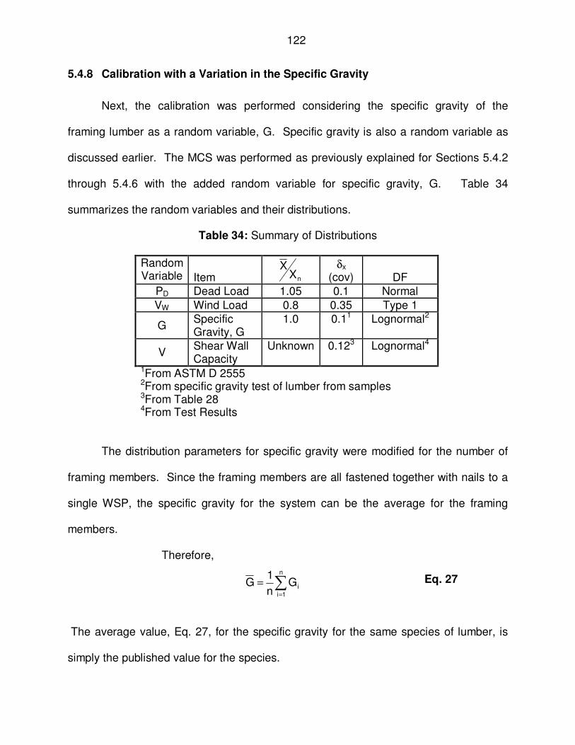
122
5.4.8 Calibration with a Variation in the Specific Gravity
Next, the calibration was performed considering the specific gravity of the
framing lumber as a random variable, G. Specific gravity is also a random variable as
discussed earlier. The MCS was performed as previously explained for Sections 5.4.2
through 5.4.6 with the added random variable for specific gravity, G. Table 34
summarizes the random variables and their distributions.
Table 34: Summary of Distributions
Random Variable Item nX
X δx (cov) DF
PD Dead Load 1.05 0.1 Normal
VW Wind Load 0.8 0.35 Type 1
G Specific Gravity, G
1.0 0.11 Lognormal2
V Shear Wall Capacity
Unknown 0.123 Lognormal4
1From ASTM D 2555 2From specific gravity test of lumber from samples 3From Table 28 4From Test Results
The distribution parameters for specific gravity were modified for the number of
framing members. Since the framing members are all fastened together with nails to a
single WSP, the specific gravity for the system can be the average for the framing
members.
Therefore,
∑=
=n
1iiG
n
1G
Eq. 27
The average value, Eq. 27, for the specific gravity for the same species of lumber, is
simply the published value for the species.

123
Assuming G1 through Gn are statistically independent and from the same
population, the variance is (Ang and Tang 1975):
= ∑
=
n
1ii2
Gn
1Var
n
1GVar )(
( )n
nn
1GVar
22
2
σ=σ=)( Eq. 28
Therefore, from Eq. 28, the standard deviation for the random variable G, is equal
to nσ , where σ is the standard deviation of the samples. Using Eq. 28, the coefficient
of variation, δ, of random variable G can be calculated as nG δ=δ , where δ is the
coefficient of variation of the samples. Using this principle, the coefficient of variation
for the wall assembly is adjusted as a weighted value. Recalling that for the test
samples, the two sole and top plates are nominally half the length of the four wall studs,
the weighted coefficient of variation is calculated as shown:
( )0450
2124
10
G
G ..
=+
=σ
=δ
Therefore, the coefficient of variation for random variable G is 0.045. For the MCS, the
coefficient of variation, 0.045, is used instead of 0.1 as indicated in Table 34.
5.4.9 Results of the Monte Carlo Simulation for ASD
As before, without the random variable G in the MCS, the results of the MCS for
the ASD load combination 0.6D+W are summarized in Table 35 for walls A, B, C, D, E
and SDPWS. For this simulation, all of the unit shear values were calibrated
considering the addition of the random variable G.
Table 35 summarizes the results as explained in Section 5.4.7 for Table 33.

124
Table 35: Summary of MCS for ASD with Specific Gravity
Calibrated Wall Values
Wall A B C D E SDPWS
Restraint, γDPD 4416 1104 2208 3312 0 5051
Ultimate Unit Shear Capacity (from tests), plf
555 345 496 615 162 786 Bias Factor, a2
1.150 0.947 0.944 1.003 1.245 1.248
Nominal Unit Shear Capacity, plf 483 363 524 613 130 629
Normalized
Phold down, λ’1 0.877 0.219 0.439 0.658 0.000 1.000
Vcap(%) 0.767 0.577 0.833 0.974 0.207 1.000
1
hCV
P
P
P
Gn
DD
SDPWSn
DD γ=
γ=λ
−
'
Just as before, a wall restrained with a hold down (wall A) only has a nominal unit
shear capacity equal to 76% of a fully restrained wall. Wall E has a nominal unit shear
capacity equal to 21% of a fully restrained wall. A curve was fit to the normalized
results of Table 35 (zunzun.com) to create a function for the partial restraint factor Cpr-n.
The equation that best fit is the Bleasdale-Nelder with offset, Eq. 25. The specific
equation that fits Table 35 is shown in Eq. 29 and is applicable for values of 0<λ’≤1.
The R2 value is 1.0 for this equation. The normalized results of Table 35, Eq. 26, and
the test results, from Graph 12, are shown graphically in Graph 32.
Partial Restraint Factor for 0 < λ’ ≤ 1,
2070163064210C 2881019257
npr .)..(./.' +λ+= −−
−
For λ’=0,
Cpn-n = 0.21
For λ’>1,
Cpn-n = 1.0
Eq. 29

125
As expected, the partial restraint function is shifted up and to the left of the actual
test result relationship. This is due to the ASD load combination requiring the use of
only 60% of the applied dead load restraining force. In other words, the actual
restraining force on the shear wall with this load combination is 167% of the factored
load, γDPD.
0%
20%
40%
60%
80%
100%
120%
0% 20% 40% 60% 80% 100% 120%
% o
f F
ull S
he
ar
Ca
pa
cit
y
% of Full Restraining Force
Test Data + APA
Holdown
Monte Carlo with G
B-N with G
Calibrated Test Data +APA
Graph 32: Partial Restraint Effect, ASD, with Specific Gravity
5.4.10 Results of the Monte Carlo Simulation for LRFD
The procedures explained for the MCS for ASD were repeated for LRFD. Since
the resistance factor, φ=0.8, is already utilized by SDPWS, the bias factor was adjusted
to calibrate the partial restraint factor for the LRFD strength values. The results of the
MCS for the LRFD load combination 0.9D+1.6W are summarized in Table 36 for walls
A, B, C, D, E, and SDPWS. The values for A, E, and SDPWS are from the FOSM

126
analysis summarized in Table 31. For these walls, the restraining force was not the limit
state of failure and was not modeled in the MCS.
Table 36: Summary of MCS for LRFD without Specific Gravity
Calibrated Wall Values
Wall A B C D E SDPWS
Restraint, γDPD 4416 1104 2208 3312 0 5051
Ultimate Unit Shear Capacity (from tests), plf
555 345 496 615 162 786 Bias Factor, a2
1.150 1.167 1.166 1.170 1.280 1.245
Nominal Unit Shear Capacity, plf 483 295 425 527 127 631
Normalized
Phold down, λ’1 0.874 0.219 0.437 0.656 0.000 1.000
Vcap(%) 0.764 0.467 0.673 0.834 0.200 1.000
1
hCV
P
P
P
Gn
DD
SDPWSn
DD γ=
γ=λ
−
'
Just as before, a wall restrained with a hold down (wall Group A) only has a
nominal unit shear capacity equal to 76% of a fully restrained wall. Wall E has a
nominal unit shear capacity equal to 20% of a fully restrained wall. A curve was fit to
the normalized results of Table 36 (zunzun.com) to create a function for the partial
restraint factor Cpr-n. The equation that best fit is the Bleasdale-Nelder with offset, Eq.
25. The R2 value is 1.0 for this equation. The specific equation that fits Table 36 is
Partial Restraint Factor for 0 < λ’ ≤ 1,
200096909500C 911215392
npr .)..(./.' +λ+= −−
−
For λ’=0,
Cpn-n = 0.20
For λ’>1,
Cpn-n = 1.0
Eq. 30

127
shown in Eq. 30 and is applicable for values of 0 < λ’ ≤ 1. The normalized results of
Table 36 and Eq. 30 are shown graphically in Graph 33.
y = -0.4982x2 + 1.294x + 0.203R² = 0.9999
0%
20%
40%
60%
80%
100%
120%
0% 20% 40% 60% 80% 100% 120%
% o
f F
ull S
he
ar
Cap
ac
ity
% of Full Restraining Force
Holdown
Monte Carlo
B-N w/o G
2nd Order Fit
Second Order Fit
Graph 33: Partial Restraint Effect, LRFD, without Specific Gravity
Although not directly comparable, the partial restraint function utilizing Eq. 30 is
extremely close to the partial restraint function shown as the second order fit equation in
Graph 29. This is due to the LRFD load combination requiring the use of only 90% of
the applied dead load restraining force. An additional second order curve was fit for
comparison to the B-N fit. The resulting curve has an R2 value of 0.9999. The equation
for the second order curve is simpler than that of the B-N curve and is presented in Eq.
31.

128
5.4.11 Calibration with a Variation in the Specific Gravity
Next, the calibration was performed considering the specific gravity of the
framing lumber as a random variable, G. This is the same as explained in section 5.4.8,
but using LRFD.
5.4.12 Results of the Monte Carlo Simulation for LRFD
As with the previous simulation, without the random variable G, the results of the
MCS for the LRFD load combination 0.9D+1.6W are summarized in Table 37 for walls
A, B, C, D, E and SDPWS. For this simulation, all of the unit shear values were
calibrated considering the addition of the random variable G.
Table 37 summarizes the results as explained in Section 5.4.10.
Almost identical to the previous simulation, a wall restrained with a hold down
(wall Group A) only has a nominal unit shear capacity equal to 77% of a fully restrained
wall. Wall E has a nominal unit shear capacity equal to 21% of a fully restrained wall. A
curve was fit to the normalized results of Table 37 (zunzun.com) to create a function for
the partial restraint factor Cpr-n. The equation that best fit was the Bleasdale-Nelder with
offset, Eq. 25. The R2 value is 1.0 for this equation. The specific equation that fits Table
Partial Restraint Factor for 0 ≤ λ’ ≤ 1,
203029414980C 2npr ... ' +λ+λ−=−
For λ’=0,
Cpn-n = 0.20
For λ’≥1,
Cpn-n = 1.0
Eq. 31
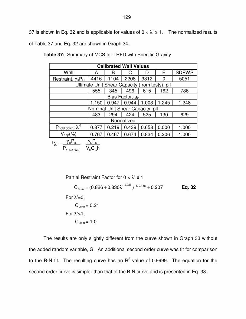
129
37 is shown in Eq. 32 and is applicable for values of 0 < λ’ ≤ 1. The normalized results
of Table 37 and Eq. 32 are shown in Graph 34.
Table 37: Summary of MCS for LRFD with Specific Gravity
Calibrated Wall Values
Wall A B C D E SDPWS
Restraint, γDPD 4416 1104 2208 3312 0 5051
Ultimate Unit Shear Capacity (from tests), plf
555 345 496 615 162 786
Bias Factor, a2 1.150 0.947 0.944 1.003 1.245 1.248
Nominal Unit Shear Capacity, plf
483 294 424 525 130 629 Normalized
Phold down, λ’1 0.877 0.219 0.439 0.658 0.000 1.000
Vcap(%) 0.767 0.467 0.674 0.834 0.206 1.000
1
hCV
P
P
P
Gn
DD
SDPWSn
DD γ=
γ=λ
−
'
Partial Restraint Factor for 0 < λ’ ≤ 1,
207083008260C 188210282
npr .)..(./.' +λ+= −−
−
For λ’=0,
Cpn-n = 0.21
For λ’>1,
Cpn-n = 1.0
Eq. 32
The results are only slightly different from the curve shown in Graph 33 without
the added random variable, G. An additional second order curve was fit for comparison
to the B-N fit. The resulting curve has an R2 value of 0.9999. The equation for the
second order curve is simpler than that of the B-N curve and is presented in Eq. 33.
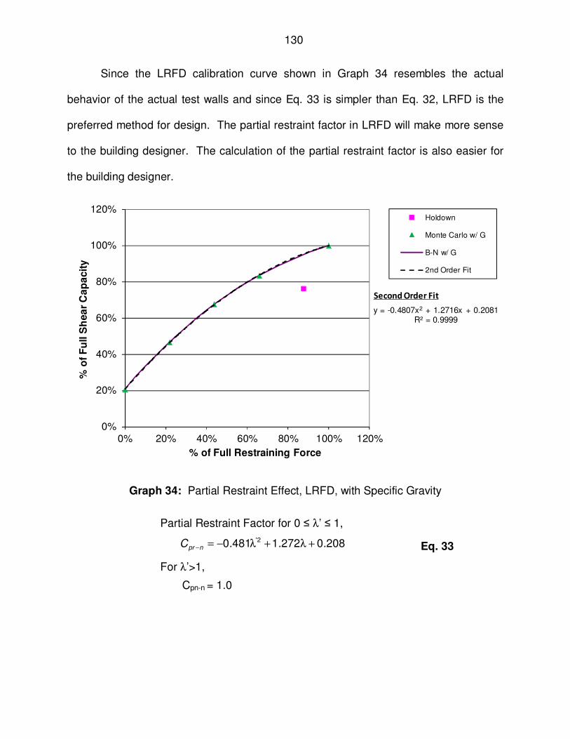
130
Since the LRFD calibration curve shown in Graph 34 resembles the actual
behavior of the actual test walls and since Eq. 33 is simpler than Eq. 32, LRFD is the
preferred method for design. The partial restraint factor in LRFD will make more sense
to the building designer. The calculation of the partial restraint factor is also easier for
the building designer.
y = -0.4807x2 + 1.2716x + 0.2081R² = 0.9999
0%
20%
40%
60%
80%
100%
120%
0% 20% 40% 60% 80% 100% 120%
% o
f F
ull S
hea
r C
ap
acit
y
% of Full Restraining Force
Holdown
Monte Carlo w/ G
B-N w/ G
2nd Order Fit
Second Order Fit
Graph 34: Partial Restraint Effect, LRFD, with Specific Gravity
Partial Restraint Factor for 0 ≤ λ’ ≤ 1,
208027214810 2 ...C 'npr +λ+λ−=−
For λ’>1,
Cpn-n = 1.0
Eq. 33

131
CHAPTER 6
DISCUSSION OF NOMINAL UNIT SHEAR VALUES
This chapter addresses some of the conflicts that exist with current methods of
determining unit shear values for wood structural panels. These conflicts directly relate
to the capacity of a partially restrained shear wall as prescribed in the IRC (2009).
6.1 Difference in Method to Determine Unit Shear Values
6.1.1 SDPWS Values for Anchoring Device
The SDPWS (2005) unit shear values, based on APA Research Report 154
(APA 2004) cannot be achieved with a conventional mechanical hold down only. The
values are reportedly based upon ASTM E72. The test frame from ASTM E72 is shown
in Figure 22. The clamping action of the test fixture is not equivalent to applying a
conventional hold down on the tension stud as explained earlier.
APA Research Report 154 (APA 2004) indicates that a timber was used over the
top of the wall and a double tie rod hold down was used to restrain the tension side of
the wall. The double tie rod system over the top of the wall provides a clamping force
keeping the wall plates in contact with the wall stud. This action keeps the plates and
stud from separating, thus reducing the force on the corner nails at the tension side.
Additionally, the second stud at each end adds additional strength and stiffness even
though the sheathing is not directly attached to it.
The conventional mechanical hold down attached to the tension stud does not
offer the same restraint as the clamping mechanism required by ASTM E72. The
elongation of the mechanical hold down allows the tension stud to separate from the

132
bottom plate and there is nothing to keep the top plate from separating from the tension
stud unless additional building framing exists. The result is the capacity of the wall is
reduced. This was observed in the test specimens and was also observed in the FE
model.
Reprinted, with permission, from ASTM E72-10 Standard Test Methods of Conducting Strength Tests of Panels for Building Construction, copyright ASTM International, 100 Barr Harbor Drive, West Conshohocken, PA 49428.
Figure 22: ASTM E72 Test Fixture
SDPWS (2005) requires either a dead load stabilizing moment or an anchoring
device at the end of the shear wall. No difference is given to either restraining device.
There is a difference between the two; the resulting unit shear strength based on the
test results shown in Table 12 with an anchoring device is 13% less or 87% of the

133
tabulated nominal unit shear value published in SDPWS (2005). Therefore, SDPWS
(2005) should at least provide an anchoring device factor, Ca, as given in Eq. 34. This
value should not be confused with the value determined in Chapter 5 which was
calibrated for design. The latter is preferred since it was calibrated to ASCE 7-05 and
the IBC (2009) load combinations to provide a reliability index, β, of 3.25.
Ca = 0.87
Eq. 34
6.1.2 Use of ASTM E72
One of the intentions of ASTM E72 is to provide a test method and a test frame
that can be used to compare different sheathing materials for use as shear walls to
resist lateral forces, such as wind loads. The standard states that it intends to function
as a shear wall that would typically be used in a building. The purpose of the standard
is to provide a relative comparison of sheathing materials.
While the stated intent of the standard is good and useful, the standard does not
capture the behavior of partially restrained shear walls that are prescribed in the 2009
IRC. It has been explained earlier that there is a large difference between a fully
restrained shear wall and a wall only restrained in accordance with the 2009 IRC.
These differences are not tested and the resulting behavior is not captured in ASTM
E72.
Due to the increased forces in the corner nails in a partially restrained shear wall,
as well as shear walls having no dead load along the top of the wall restrained with a
hold down, wall sheathing intended as shear wall material should be tested to capture

134
this behavior. This will provide a relative comparison of different materials. The
behavior of the sheathing material at the edges can be crucial to the strength of the wall
and in fact was the focus of the research conducted by Cassidy (2002).
ASTM E72 recognizes that a prestress force can greatly influence the results of
the racking test and restricts the prestress in the hold down rods to 20 lb. However,
there is no requirement to report the initial hold down force or the hold down force
throughout the test. Reporting of this data should be made so that the entire test
method to determine the resulting unit shear values is completely transparent if these
values will be used in design standards. This too will allow for a comparison of different
sheathing materials.
6.1.3 Use of ASTM E564
ASTM E564 states that its use is not intended for classifying sheathing shear
capacity. Thus, to this author’s knowledge, it is not used in the design standards. In
contrast to ASTM E72, ASTM E564 allows for walls to be constructed in dimensions
intended for use and with the boundary conditions and restraining forces of the intended
use. This results in data that reflects the actual construction of the wall and doesn’t
attempt to only make a relative comparison of sheathing material shear capacity as
ASTM E72 does.
Since the failure of wood shear walls is highly dependent on the capacity and
response of the fasteners as well as the initial boundary conditions, it makes sense to
use ASTM E564 for codified design standards for partially restrained wood shear walls.
This standard was used as the basis of the testing for this thesis as well. This would

135
also provide a relative comparison of sheathing material performance where edge
breakout or failure is the limit state.
6.1.4 Partial Restraint Factors
It is obvious that the peak capacity of wood shear walls in a fully restrained
condition is greater than the peak capacity of a wood shear wall with a mechanical hold
down at the base of the wall. Therefore, when a wall is partially restrained from the top,
the partially restrained capacity must be a function of the fully restrained condition (i.e.
the APA Research Report 154 ultimate capacity) rather than the nominal (SDPWS –
unless it is calibrated) capacity, or the mechanical hold down restrained capacity. This
is best shown in Graph 35 where the partial restraint effect from this research is
compared with Ni and Karacabeyli’s (2000).
As explained earlier in Chapter 2, Ni and Karacabeyli (2000) assumed that a wall
with a mechanical hold down at the base of the wall was fully restrained. As shown in
Graph 35, there is a noticeable difference when using this assumption. The light scale
represents Ni and Karacabeyli’s (2000) partial restraint factor and partial restraint force.
Their curve was scaled to the hold down capacity from this research to make the
comparison.
Another problem with using the unit shear capacity developed with a mechanical
hold down as the fully restrained unit shear capacity is that this capacity is unknown
unless testing is conducted or unless a partial restraint factor for a mechanical hold
down is used as proposed in this research. Therefore, a correlation must always be
made to between the unit shear capacity with a mechanical hold down and the nominal
value in SDPWS (2005).

136
0%
20%
40%
60%
80%
100%
120%
0% 20% 40% 60% 80% 100%
% o
f F
ull S
hear
Cap
ac
ity
% of Full Restraining Force, λλλλ
Partial Restraint Effect on Strength
Test Data + APA
Holdown
SDPWS Nominal
Ni and Karacabyli
Poly. (Test Data + APA)
20% 40% 60% 80% 100%
20%
40%
60%
80%
100%
Graph 35: Comparison of Partial Restraint

137
CHAPTER 7
SUMMARY, CONCLUSION, AND RECOMMENDATIONS FOR FUTURE RESEARCH
7.1 Summary
The unit shear capacity of partially restrained WSP shear walls constructed in
accordance with the 2009 IRC was studied in this thesis. A nonlinear finite element
model was developed to understand and describe the behavior of these walls.
Additionally, as a focus of this thesis, a reliability analysis was conducted to develop
modification factors to fully restrained unit shear capacities. These modification factors
were calibrated to provide a uniform reliability index of 3.25.
7.2 Conclusions
The following conclusions are made from this research effort:
1. The SDPWS (2005) nominal unit shear capacity, 730 plf, for 15/32” WSP with
8d common nails at 6” o.c. at the perimeter and 12” o.c. at the intermediate
members provides a reliability index, β=3.25, for wind load using the ASD
reduction factor of 2 per SDPWS (2005) and using the LRFD resistance factor
of 0.8. This was used as the target reliability index for the calibration.
2. The derivation of design values for use in SDPWS with ASTM E72 is not
appropriate for walls anchored with mechanical hold downs or partially
restrained IRC (2009) prescriptive walls. The ASTM E72 test frame provides
a clamping action not present in partially restrained shear walls. ASTM E564
is appropriate for shear walls with these types of restraint.
138
3. ASTM E72 should add a requirement to record the initial and resulting hold
down force for a racking test. Though it has a limit of a maximum 20 lb of
initial hold down force, it does not have to be measured for the test.
4. The SDPWS (2005) nominal unit shear capacities, based on APA Research
Report 154 (APA 2004), cannot be achieved with a conventional mechanical
hold down at the base of the wall for a 4’ x 8’ WSP shear wall.
5. For the ASD design methodology, partially restrained shear walls have an
allowable nominal unit shear capacity to resist wind load, V’n, as shown in
Eq. 35. This is applicable to 4’ x 8’ WSP shear walls constructed in
accordance with the IRC (2009) using a mechanical hold down device (i.e.
Simpson HUD14) at the base of the wall.
ASD
Gan'
nC
CCVV =
Where,
Vn = nominal unit shear capacity per SDPWS (2005) Ca = anchor reduction factor Ca = 0.77 CG = 1-(0.5-G) G = specific gravity of the framing lumber CASD = 2
Eq. 35
6. For the ASD design methodology, wood shear walls partially restrained by a
dead load restraining force, P, have a nominal unit shear capacity to resist
wind load, V’n, as shown in Eq. 36. The controlling IBC (2009) load
combination is 0.6D+W. This is applicable to 4’ x 8’ WSP shear walls
constructed in accordance with the IRC (2009).

139
ASD
Gprn'
nC
CCVV =
Where, Vn = nominal unit shear capacity per SDPWS (2005)
2070163064210 09709257.)C..(C ..
ppr ++= −−
CG = 1-(0.5-G) G = specific gravity of the framing lumber
01C 01
0C 2070
01C0 hCV
P
p
p
p
Gn
.;.C
;.C
.;C
p
p
p
≥=
==
≤<=
h = height of shear wall P = 0.6PD [per IBC (2009)] (restraining force) CASD = 2
Eq. 36
7. For the LRFD design methodology, partially restrained shear walls have an
allowable nominal unit shear capacity to resist wind load, φV’n, as shown in
Eq. 37. This is applicable to 4’ x 8’ WSP shear walls constructed in
accordance with the IRC (2009) using a mechanical hold down device (i.e.
Simpson HDU14) at the base of the wall.
Gan
'
n CCVV φ=φ
Where,
φ = strength reduction factor φ = 0.8 Vn = nominal unit shear capacity per SDPWS (2005) Ca = anchor reduction factor Ca = 0.77 CG = 1-(0.5-G) G = specific gravity of the framing lumber
Eq. 37
8. For the LRFD design methodology, wood shear walls partially restrained by a
dead load restraining force, P, the nominal unit shear capacity, φV’n, as
shown in Eq. 38. The controlling IBC (2009) load combination is

140
0.9D + 1.6W. This is applicable to 4’ x 8’ WSP shear walls constructed in
accordance with the IRC (2009).
Gprn'n CCVV φ=φ
Where, φ = strength reduction factor φ = 0.8 Vn = nominal unit shear capacity per SDPWS (2005)
208027214810 2 .C.C.C pppr ++−=
CG = 1-(0.5-G) G = specific gravity of the framing lumber
01C 01
0C 2080
01C0 hCV
P
p
p
p
Gn
.;.C
;.C
.;C
p
p
p
≥=
==
≤<=
h = height of shear wall P = 0.9PD [per IBC (2009)] (restraining force)
Eq. 38
9. The curve generated by the partial restraint factor, Cpr, in Eq. 38 (LRFD
method) more accurately emulates the actual shear wall behavior than the
same factor in Eq. 36 (ASD method). The ASD controlling load combination
creates a shift in the curve of the partial restraint factor due to use of only
60% of the dead load restraining force.
10. The IRC (2009) assumption that shear walls are partially restrained requires a
dead load force applied to the top of the shear wall at the tension side as
indicated in Table 38.
Table 38: Design Restraining Force for IRC Shear Wall
Wall Supporting IRC Partial-Restraint Factor
Dead Load Required (lb)1
Roof Only 0.8 2,786 Roof + One Story 0.9 3,512
Roof + Two Stories 1.0 6,867 1Based on 3/8” WSP per IRC with SPF Framing, G=0.42

141
11. The clamping force in shear walls constrained from the top with either
external mechanical methods or dead loads allows a substantial horizontal
load to transfer through the studs to the plate (220 plf for this research). For
this reason, the nails in the vertical end studs always failed first for these
types of shear walls. This behavior is not realized without the clamping
action.
12. Finite element analysis should model the behavior of wood shear walls. It
should always include the effect of the boundary conditions and should model
the connection behavior of the studs to the plates. The separation of the
studs from the plate can greatly reduce the unit shear capacity of the wall.
7.3 Recommendations for Future Research
Future research could extend in a number of directions. Since the coefficient of
variation for wind load is so large, this is an area that could use further research.
Additional research could be conducted on the effect of wall length on partially
restrained walls. This could be included as a parameter to the partial restraint
modification factor if it is found to be significant. Finite element modeling could be
improved with further research on connections within the shear wall. Particularly the
interaction of nail withdrawal and shear resistance of the framing nails. Upon improving
the connection behavior in FEM, comparisons of whole building tests utilizing partial
restraints can be made and the FEM can be further calibrated.

142
APPENDIX A
WALL TESTS
A1 Wall Testing
This appendix details further the testing procedure conducted for the 25 wood
shear wall tests.
A2 Wall Materials
The material was delivered to the lab on March 11, 2011. The following material
was received and inventoried:
Table 39: Lumber Materials
Quantity Description
100 2x4x925/8” SPF NSLB1 Stud Grade Precut Studs 25 2x4x14’ SPF NLGA2 No. 2 Plate Material 25 32/16 APA Rated Sheathing, ½” Category
Oriented Strand Board (OSB), tmin=0.483” 1National Lumber Softwood Bureau; SPF South, G=0.36 2National Lumber Grades Authority; SPF North, G=0.42
Photo 2, Photo 3, Photo 4 and Photo 5 show the stamps recorded from the material.
The 2x4x14’ plate material was cut into three pieces each 49½” long for the wall
plates. The groups of three plates were maintained such that all three plates from the
same 14’ board were used in one wall. During the cutting procedure, the 16” o.c. stud
locations were marked. After cutting all of the plates, a ¾” diameter hole was drilled in
each bottom plate, five at 3” from one end and twenty 12” from one end. The former

143
was for the Group A walls with the hold down while the latter was for the 5/8” diameter
anchor bolt for Groups B to E.
The OSB sheathing was further inventoried by weighing each piece, measuring
the thickness of each side of each piece, marking the wall number, marking the nail
locations, and performing an out-of-plane stiffness test on each piece. Each sheet was
Photo 2: Wall Stud
Photo 3: Wall Plate
Photo 4: OSB Sheathing
Photo 5: OSB Sheathing
Photo 6: Digital Scale for OSB
Photo 7: Digital Scale Monitor
Photo 8: Thickness of OSB

144
carefully weighed with a Pelouze Model 4010 digital scale to one-tenth of a pound,
Photo 6 and Photo 7 recorded. The thickness of each side of each sheet was
measured with a dial caliper to 0.001” along with two pieces of 3/8” x 5/8” x 4” tool steel
Photo 7. The tool steel was used to provide an average thickness of the OSB. Some of
the wood flakes are thicker than others creating high and low areas. The tool steel
averaged these high and low areas allowing a more accurate measurement. The
identification was marked on each sheet of OSB Photo 9. Next, each sheet was placed
on a pair of sawhorses spaced 7’- 8½” apart, center-to-center, and tied together with a
pair of 2x4 strong-backs. The location of the sawhorses was marked on the floor as a
reference.
The nail locations were marked on the face of each sheet using a piece of OSB
as a story pole Photo 10. An out of plane stiffness test was also conducted as a way to
compare each sheet against one another. The test was conducted simply by supporting
each end of each piece of OSB such that it was spanning the long, 8 ft, length. Once
the sheet was set in the fixture, the center was
marked. An initial measurement from the long edge
was made at the center of the length (measured and
marked) to the concrete floor below (square to the
Photo 9: Wall Identification
Photo 10: Nail Layout
Photo 11: Panel Stiffness

145
floor and marked on the floor). After
the initial measurement, a 41.4 lb
weight was added to the center of the
sheet and another measurement was
made to the floor below, Photo 11.
These measurements were recorded to
obtain a flexural stiffness. The results
of the OSB measurement are
summarized in Table 40.
A3 Wall Construction
After inventorying the lumber
and preparing it for construction of the
wall, a fixture, Photo 12, was
constructed to fabricate each wall. The
fixture consisted of a pair of sawhorses
with LVLs and 2x4s connecting them
and forming stops to construct square
walls. Each wall consists of three
plates (two on top and one on bottom), four studs, and one sheet of OSB.
Table 40: OSB Measurements
Weight OSB Sample
Average Thickness
Estimated Stiffness
(lbs) (in) (lb-in2/ft)
A1 50.8 0.523 152,009
A2 51.2 0.529 152,009
A3 52.4 0.534 156,912
A4 50.0 0.515 135,119
A5 51.2 0.533 152,009
B1 51.2 0.519 143,067
B2 50.0 0.510 135,119
B3 50.6 0.505 152,009
B4 50.8 0.511 147,403
B5 51.2 0.527 152,009
C1 52.2 0.526 152,009
C2 51.4 0.529 162,143
C3 52.2 0.529 162,143
C4 52.0 0.525 156,912
C5 51.8 0.519 156,912
D1 52.2 0.534 167,734
D2 51.0 0.513 147,403
D3 51.0 0.523 162,143
D4 53.2 0.538 147,403
D5 50.0 0.530 156,912
E1 53.2 0.534 135,119
E2 52.0 0.525 135,119
E3 53.2 0.535 135,119
E4 50.6 0.533 187,088
E5 52.8 0.549 152,009
Minimum 50.0 0.505 135,119
Maximum 53.2 0.549 187,088
Average 51.5 0.526 151,753
Variance 0.98 0.000 143,766,517
Std. Dev. 0.99 0.010 11,990
COV 0.02 0.02 0.08

146
To begin construction of the walls, the bottom plate and one top plate were
placed in the fixture. Next, four studs were placed between the plates at the previously
marked locations on the plates. The bottom plate was fastened to each stud, Photo 13,
with 2-0.131”x3¼” smooth shank, full head nails, Photo 14 and Photo 15, with a
Paslode pneumatic nail gun. The top plate was fastened to each stud the same as the
bottom plate. Next, the OSB wall sheathing was placed atop the studs and plates. The
bottom edge was carefully aligned with the bottom edge of the bottom plate and the
stud frame was blocked tight to the fixture to square it. A gage block was made to hold
the edge of the sheathing ¾” from the edge of the end studs, Photo 16. The aligned
sheathing on the stud framed wall is shown in Photo 17. Once the sheathing was
Photo 12: Wall Fixture
Photo 13: Wall Stud Connection
Photo 14: Stud Fasteners
Photo 15: Stud Fasteners
Photo 16: OSB Edge Gage
Photo 17: Assembled Wall

147
aligned in the correct position and the wall was square, the sheathing was fastened to
each stud with 8d Common (0.131”x2½” smooth shank, full head) nails, Photo 18 and
Photo 19, with a Paslode pneumatic nail gun, Photo 20.
For all nails, the nail gun depth, Photo 21, and air pressure was set so that the
nail heads were set flush with the surface of the material, Photo 22 and Photo 23. In
instances where the nail was not fully driven, the nails were driven flush with a hammer.
No fasteners were overdriven. The placement of the fasteners was accomplished with
accuracy as shown in Photo 23. Along the vertical edges, the fasteners were located
Photo 18: Sheathing Fasteners
Photo 19: Sheathing Fasteners
Photo 20: Pneumatic Nailer
Photo 21: Nail Depth Adjustment
Photo 22: Sheathing Fastener Placement
Photo 23: Sheathing Fastener Placement
Photo 24: Edge Blow Out
Photo 25: Relocated Nail at Damaged
Edge

148
3/8” from the edge of the sheathing and 3/8” from the inside edge of the stud, Photo 22.
At these locations, the fasteners were driven at an angle (about 5°). After completing
the fastening of the sheathing, the back side was checked for any nails that missed the
studs. If any nails missed, they were removed and a new nail was installed 1” away
from the intended location. Similarly, if the edge of the sheathing was damaged (edge
blow out), Photo 24, the nail was removed and a new nail was installed 1” away from
the intended location, Photo 25. These instances did not occur very often and the
avoidance skills were learned after two walls. Consistency of construction was easily
accomplished since all walls were constructed the same day, in the same fixture, and by
the same person.
For all of the walls, the sheathing fastening was the same. The perimeter nails
were placed 6” o.c. (except first and last spaces) and the intermediate member nails
were placed at 12” o.c. (except first and last spaces). The spacing at the first and last
space was different to allow for the boundary condition. If the same spacing was used,
the nails would be at the edge of the sheathing. As noted above, the nails along the
vertical edges were place 3/8” from the edge of the sheathing. The nails along the
bottom plate were placed ¾” from the bottom edge of the sheathing or along the
centerline of the bottom plate. The nails along the top edge were placed along the
centerline of the first top plate, or 11/8” from the top edge of the sheathing. Since there
was no need to maintain a 3/8” edge distance on the corner nails, they were installed ¾”
from the vertical edge, Photo 20.
For the Group A walls, a mechanical hold down was installed to create the
restrained condition. A Simpson HDU8 hold down was used for wall A5, Photo 26. The
149
HDU8 was installed flush with the bottom plate, Photo 27, and fastened to the stud with
20-SDS ¼”x2½” screws, Photo 28. Since the screws were longer than the stud
thickness of 1½” a nominal 20” long 2x4 scab was used on the outside face of the stud,
Photo 27, so that the SDS screws could fasten to it as well. No other fasteners were
used between the scab and the stud. The bottom of the scab was held 5¼” up from the
bottom of the wall. This was duplicated for the remaining Group A walls.
After testing wall A5, it was determined that the flush installation of the hold down
caused prying of the bottom plate at the end stud. This was discussed earlier in
CHAPTER 3. For this reason, the hold down was held up 1” from the bottom plate on
walls A1 to A4, Photo 29. Also, the hold down was changed to a Simpson HDU14 hold
down, Photo 30, for these remaining walls. This was done to assure that the wall failure
would not be a result of the hold down or hold down fastener slippage. The HDU14 was
installed 1” above the bottom plate and fastened to the stud with 36-SDS ¼”x2½”
screws. The Simpson catalog states “Tension values are valid for hold downs flush or
raised off of sill plates.” They do not indicate a preferred method for installation.

150
Photo 26: Simpson HDU8 Hold Down
Photo 27: Simpson HDU8 Hold Down
Photo 28: SDS ¼” x 2½” Screw
Photo 29: Simpson HDU14 Hold Down
Photo 30: Simpson HDU14 Hold Down
A4 Test Setup
A4.1 Test Fixture Setup
The test fixture was setup within the Structural Building Component Research
Institute’s test lab. The fixture was fabricated such that each wall specimen could be
easily removed and the next one installed. An overall view of the test fixture setup is
shown in Figure 23.

Figure 23: Test Setup
1
2
3
4
5 6 7 8 9 11 10
13 12
15 14
17 16
18
19
Key: 1. Horizontal actuator 2. Vertical actuator 3. Horizontal actuator load
cell 4. Vertical actuator load
cell 5. Horizontal load cell 6. Vertical load cell at stud 7. Vertical load cell at stud 8. Vertical load cell at stud 9. Vertical load cell at
holdown 10. Horizontal string pot at
base of sheathing (front)
11. Horizontal string pot at bottom plate (back)
12. Vertical string pot at base of sheathing (front)
13. Vertical string pot at bottom plate (back)
14. Vertical string pot at base of sheathing (front)
15. Vertical string pot at bottom plate (back)
16. Horizontal string pot at top of sheathing (front)
17. Horizontal string pot at top plate (back)
18. Diagonal string pot (back)
19. Wall test specimen
15
1

152
A4.2 Test Frame
The test frame utilized two portal test frames and one cantilevered column. All
columns were W36x135’s which were anchored to a strong floor. The two portal frames
were used to support the vertical actuator utilizing a W6x25 beam supported by
brackets on the columns. The W6x25 was installed parallel to the columns. The
cantilevered column was used to support the horizontal actuator. This column was
oriented 90° to the portal columns.
The base of the test frame consisted of an HSS6x2x¼ welded to bearing plates
Photo 31: Base Roller
Photo 32: Base Bearing Plate
Photo 33: Alignment of Frame
Photo 34: Alignment of Frame
Photo 35: Alignment of Horizontal Actuator
Photo 36: Restraint of Actuators

153
that were anchored to the strong floor. This tube supported four roller bearings, Photo
31, one below each wall stud. The roller bearings consisted of two steel rollers atop the
tube and two nylon rollers along the bottom, below the tube. Therefore the rollers could
resist compression and tension forces. A load cell with a bearing plate was mounted on
each roller, Photo 32.
The HSS6x2 was aligned with the W6 above using a plumb bob and both were
parallel with the portal frame columns. The plumb bob was also used to set the vertical
actuator, Photo 33 and Photo 34. The horizontal actuator was aligned with a string
along the centerline of the wall and leveled in place, Photo 35. Both vertical and
horizontal actuators were anchored to resist translation at the wall, Photo 36
The actuators were both hydraulic piston, 25,000 lb capacity, with a 20” stroke.
The actuators each have internal load cells and LVDT’s for control. The vertical
actuator was connected to a roller where it loaded the wall, Photo 38 and Photo 39.
This was the same roller as the base of the wall but with the nylon rollers removed. The
horizontal actuator had a 1½” diameter T-bar that pushed against the wall bar. This T-
bar was smooth to slide on the wall bar.
In order to transfer the load from each actuator to the wall, a T-shaped steel
bracket was fabricated from HSS3x2x¼ steel. An additional ½” plate was added to the
vertical piece of the T-shaped bracket to bear against the ends of the double top plate,
Photo 40. This was done to keep the load on the double top plates and not load the
end stud. The T-shaped bracket was also necessary to allow the wall to rotate and the
actuators to slide on corner of the wall. To eliminate adding additional stiffness to the
wall, the bracket only extended to the second stud. The bracket was fastened to the top

154
plate with 2-¼ x 3” screws. The surface of the T-
shaped bracket was smoothed with a belt sander to
minimize friction on the T-bar.
The wall was restrained at the top to resist out
of plane movement by adding two 2x4 strong-backs (two 2x4’s fastened in an L-shape)
with two rollers each. The strong-backs were fastened to the top of the wall with
2-¼ x 3” screws. The rollers were guided along an L5x5x¼ parallel to the wall and
anchored to the portal frame columns as shown in Photo 37. The rollers were offset
down 3” from the strong-backs to allow the rollers to be in contact with the guide as the
wall rotated and moved upward. The strong-backs were skewed to the wall so that
each roller is in contact with the guide. A 2x4 gauge block was placed between the top
of the wall and the guide to locate the wall in the correct position (parallel to the guide)
before fastening the strong-backs to the top of the wall.
Photo 37: Guide Rollers
Photo 38: Alignment of Vertical Actuator
Photo 39: Vertical Actuator Roller
Photo 40: Horizontal Actuator

155
A5 Instrumentation
The wall test specimen was instrumented as shown in Figure 23. A total of seven
load cells were used and nine string potentiometers. The load cells measured both the
actuator loading and the reactions. The string potentiometers captured the global
displacement of the wall both vertically and horizontally by measuring the wall studs and
plates. The global displacement of the sheathing was measured as well.
Measurements at the two locations allow for the determination of the differential
movement of the sheathing. A diagonal measurement of the wall was also made on the
back side of the wall studs.
The equipment used for the tests is shown in Figure 23 and summarized in Table
41. A typical load cell is shown in Figure 24. A typical sting potentiometer is shown in
Figure 25. The load cells and string potentiometers were all calibrated between
September 24, 2010 and October 6, 2010. Each calibration had a text file that was
imported into the data acquisition software. The calibrations of the string
potentiometers were nonlinear.
A total of 17 channels were connected for the data acquisition, but only 16 were
used; items 3-18 in Figure 23. The data acquisition equipment, Photo 41, was then
connected to a desktop CPU, Photo 42, for processing and recording.
All of the string potentiometers, except the diagonal one, were connected to rigid
fixtures. The two string potentiometers used to measure vertical displacement of the
OSB sheathing were connected to a gate that could swing out of the way for the wall
exchange. The string potentiometers were connected to the wall specimen with wood

156
screws that were installed in the same location for each wall, Photo 43. This allowed for
quick set up of each wall.
Table 41: Test Equipment
Function Model Displacement Measurements-
• Micro-Epsilon String Potentiometers WDS-500-P60-SR-U WDS-7500-P60-SR-U WDS-1500-P60-SR-U
Load Actuator • Hydraulic Piston • 20” Stroke Maximum • 25,000 lb Load Maximum
Load Cells • Interface Load Cells • Eccentric Load Compensated • Tension and Compression Capacity • Performance to 0.02% Error
1210 AF-10K-B & 1220 DRB-25K
Data Acquisition • Up to 1,000,000/# of Measuring
Devices Hz
Figure 24: Load Cell
Figure 25: String Potentiometer

157
A total of 17 channels were connected for the data acquisition, but only 16 were
used; items 3-18 in Figure 23. The data acquisition equipment, Photo 41, was then
connected to a desktop CPU, Photo 42, for processing and recording.
A5.1 Test Equipment Software
Two separate software programs were used to conduct the test; one for the data
acquisition and one for the actuator control. The data acquisition software used was
Dasylab 10. This software had a wonderful interface that allowed pasting images of the
test setup, created with AutoCAD, into its graphic view. Then, text boxes were created
at each of the instruments that were linked to the instruments. This allowed real time
views of the load and displacement that could quickly be identified on the graphic.
Additionally, the load-deflection curve was plotted real time as well. The plot included
Photo 41: Data Acquisition
Photo 42: CPU For Recording Data
Photo 43: String Potentiometer Connection

158
both the stud and the sheathing displacement. It was easy to see the peak load with
this plot of the hysteresis curve. The peak load was also displayed on the screen along
with the calculated unit shear in the wall panel. Figure 26 shows a view of the graphics
display from Dasylab. The actuator control software used was Adamation. This
software controlled the actuators during the test as well as allowed manual control of
the actuators during the test setup. The load protocol was entered into the software in a
spreadsheet format, Figure 27. This allowed easy changes for the five different load
test setups. The manual control allowed the user to retract the actuators when the test
was complete and then bump them into the wall after the new wall was installed in the
test assembly. The software also allows the user to set a maximum load that can be
applied in manual mode for safety. This limit was set to 40 lb for this testing.
Figure 26: Data Acquisition Software Graphics Display

159
A5.2 Test Procedure
A5.2.1 Test Sequence
The testing followed the alpha order indicated in Table 11. The purpose of this
was to determine the hold down force from the Group A wall set and consider this as
the full restraining force. The subsequent groups then used a fraction of this restraining
force as indicated in Table 11.
A5.2.2 Test Loading
As described earlier, the five walls in Group A were restrained with a hold down.
Each wall was placed in the test fixture tight against the lateral load cell at the base of
the wall; the hold down bolt was installed through the hold down and into the load cell
below; the top of the wall was supported with the two roller guides; the T-bar was
connected to the top of the wall; the other two bottom load cells were aligned with the
Figure 27: Actuator Control Software Load Steps

160
Graph 36: Wall Group A Loading
Test Load Steps
0
1000
2000
3000
4000
5000
6000
0 500 1000 1500 2000 2500 3000 3500
Time t, sec
Lo
ad
P, lb
Load Step
Limit actuator to a
maximum load of
5,000 lb
Typical Load
Rate=5.71 lb/sec
two interior studs; all string potentiometers were connected to the wall; and the
horizontal actuator was placed up against the T-bar with a nearly zero force.
The loading for the wall specimen was based on ASTM E564. The load was
applied in load steps as indicated in Graph 36. This illustrates the load steps that were
entered into the actuator control software as shown in Figure 27. Load step one is the
preload which was 10% of the estimated ultimate load and was applied for 5 minutes.
Load steps two and three were at 1/3 and 2/3 the estimated ultimate load respectfully
and are applied for 1 minute. Load step four was the final load step to determine the
ultimate capacity. The load rate for each of the load steps was the same and was
determined from the estimated ultimate load applied over a period of seven minutes.
ASTM E564 requires the load to be applied in no less than five minutes. As shown in
Graph 36 each of the first three load steps were unloaded at twice the loading rate.

161
The actuator was load controlled instead of deflection controlled. This was used
because the actuator control software can either provide load control or displacement
control. For two actuators, the control type must be the same. In other words, the
vertical actuator could not be load controlled while the horizontal actuator was
displacement controlled. Since the vertical actuator had to be load controlled, the
horizontal actuator also was load controlled. The tests were typically manually stopped
since the limit load was always well above the anticipated ultimate load.
The data for the tests was recorded by the data acquisition equipment. This
recorded the load cell and string potentiometer data. The rate at which the data was
recorded was two readings every second or 2 Hz.
Subsequent tests using ¼, ½, and ¾ of full restraint, and no restraint were
conducted as Groups B, C, D and E respectively. The restraining forces for the partially
restrained tests was provided by the vertical load actuator placed above the end of the
wall with a load cell between the actuator and the wall to obtain the actual applied
restraining force as shown in Figure 23. As noted earlier the unrestrained wall had one
5/8” diameter anchor bolt 12” from the tension end and no load from the actuator above.
A5.2.3 Test Procedure
Once the test specimen was set and ready, the load cells and string
potentiometers were zeroed on the data acquisition software and the software was set
to record to a previously named text file in a project folder. Each filename and folder
was unique for each test. The filename for each wall was of the same format so that it
could be processed with Matlab software afterward. The load test was then started
from the actuator control software.

162
Once the test began, the specimen was monitored for stability and performance
and the data acquisition software display, Figure 26, was monitored for expected
behavior. The data acquisition software display made it easy to see that the load cells
and string potentiometers were working and that the readings were making sense
based on the load input and displacement.
The project folder on the computer was checked regularly to make sure that the
data text file was being written by the data acquisition software. During the test, notes
and screenshots from the data acquisition software display were added to a unique
word processing file for each wall specimen. The file used the same format so that it
was easy to analyze the data afterward.
A5.2.4 Test Data
The test results were in the form of an ASCII text file. The file records the date
and time of each reading. The readings were of the sixteen channels shown as items 3-
18 in Figure 23. As noted earlier, the instrumentation readings were taken at a rate of 2
Hz. In addition to the data acquisition, photos of the wall after failure were also taken.
The photos aided in recording the failure modes of the particular walls. In addition to
the photos, video of the bottom plate on the tension side was taken on seven of the
partially restrained and unrestrained wall specimens.

163
A6 Specific Gravity Test
The specific gravity of the studs,
plates, and wall sheathing was
determined with a specific gravity test in
accordance with ASTM 2395. Upon
completion of the tests, the wall
specimens were dismantled and
oversized specific gravity test specimens
were cut from each individual piece,
identified with a marker for the wall specimen and the location of the member in the wall
specimen. The samples were immediately sealed in plastic bags, Photo 44 for
transportation from the SBC Research Institute to the test lab.
The samples were then cut to
uniform sizes with square edges for
volume measurements. The samples for
the 2x4’s were cut to 1 in. lengths (parallel
to grain) and the wall sheathing was cut to
3 by 6 in. pieces. Each piece was identified as described above, measured, and
weighed, Photo 45. The size measurements were made with a dial caliper with a
precision of 1/1000 in. The weight of each sample was made with an AccuLab Pocket
Pro 150-B digital scale with an accuracy of 0.1 g. The samples were all resealed in their
plastic bags until they were oven-dried.
Photo 44: Specific Gravity Samples from Wall Specimens
Photo 45: Scale and Calipers
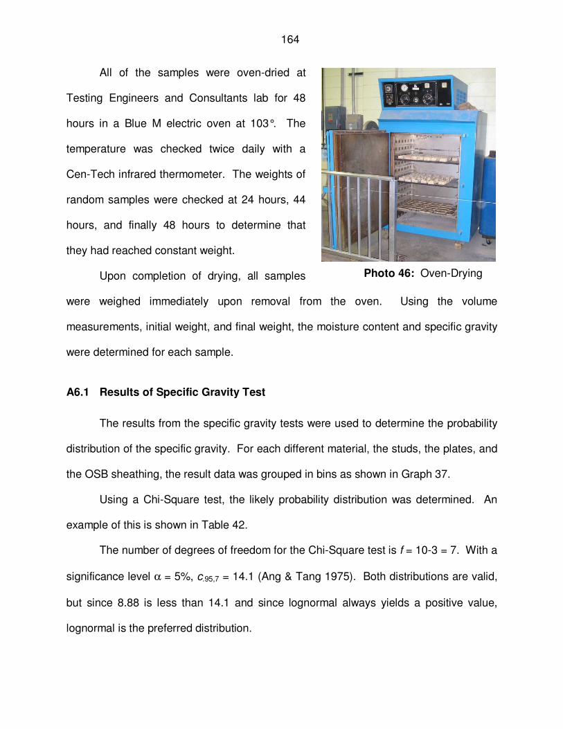
164
All of the samples were oven-dried at
Testing Engineers and Consultants lab for 48
hours in a Blue M electric oven at 103°. The
temperature was checked twice daily with a
Cen-Tech infrared thermometer. The weights of
random samples were checked at 24 hours, 44
hours, and finally 48 hours to determine that
they had reached constant weight.
Upon completion of drying, all samples
were weighed immediately upon removal from the oven. Using the volume
measurements, initial weight, and final weight, the moisture content and specific gravity
were determined for each sample.
A6.1 Results of Specific Gravity Test
The results from the specific gravity tests were used to determine the probability
distribution of the specific gravity. For each different material, the studs, the plates, and
the OSB sheathing, the result data was grouped in bins as shown in Graph 37.
Using a Chi-Square test, the likely probability distribution was determined. An
example of this is shown in Table 42.
The number of degrees of freedom for the Chi-Square test is f = 10-3 = 7. With a
significance level α = 5%, c.95,7 = 14.1 (Ang & Tang 1975). Both distributions are valid,
but since 8.88 is less than 14.1 and since lognormal always yields a positive value,
lognormal is the preferred distribution.
Photo 46: Oven-Drying

165
Sawn Lumber Specific Gravity Histogram
-2
0
2
4
6
8
10
12
14
16
18
0.2 0.25 0.3 0.35 0.4 0.45 0.5 0.55 0.6
Fre
qu
en
cy
Graph 37: Distribution of the Specific Gravity for SPF-S Studs
Table 42: Chi-Square Test for Specific Gravity Probability Distribution for Studs
Chi-Square Test for Relative Goodness-of-fit
Theoretical frequency
ei (ni-ei)
2/ei
Interval
Observed frequency
ni Normal Lognormal Normal Lognormal
<0.3 0 2.9 2.0 2.89 2.04
0.3-0.32 6 6.7 6.8 0.07 0.09
0.33-0.34 15 14.1 15.4 0.06 0.01
0.34-0.36 32 21.2 22.4 5.44 4.08
0.36-0.38 17 22.9 22.4 1.51 1.31
0.38-0.40 17 17.6 16.2 0.02 0.04
0.40-0.42 7 9.6 8.9 0.72 0.41
0.42-0.44 3 3.8 3.9 0.15 0.19
0.44-0.46 2 1.0 1.4 0.86 0.30
>0.46 1 0.2 0.5 2.39 0.41
Σ 100 100.0 100.0 14.10 8.88

166
OSB Sheathing Specific Gravity Histogram
0
1
2
3
4
5
6
7
8
0.48 0.50 0.52 0.54 0.56 0.58 0.60 0.62 0.64 0.66
Fre
qu
en
cy
OSB Specific Gravity
Graph 38: Distribution of the Specific Gravity for OSB Sheathing
The specific gravity of the materials for the five sets of walls are shown in the
following tables .

167
Table 43: Specific Gravity of Members in Wall Group A
A1 A2 A3 A4 A5G G G G G
1 0.33 0.34 0.35 0.38 0.45
2 0.33 0.35 0.40 0.34 0.323 0.31 0.37 0.36 0.31 0.37
4 0.39 0.36 0.35 0.42 0.35BP 0.36 0.40 0.42 0.36 0.40
TP 0.37 0.39 0.42 0.36 0.39TP.2 0.37 0.39 0.47 0.37 0.39
G 0.56 0.50 0.57 0.62 0.60t, in 0.510 0.506 0.513 0.495 0.498
Set "A" with HoldownWall
Member
OSB
Table 44: Specific Gravity of Members in Wall Group B
B1 B2 B3 B4 B5G G G G G
1 0.33 0.35 0.36 0.34 0.34
2 0.35 0.39 0.35 0.36 0.343 0.45 0.40 0.38 0.36 0.34
4 0.40 0.32 0.40 0.35 0.38BP 0.38 0.43 0.39 0.43 0.37
TP 0.38 0.41 0.39 0.43 0.36TP.2 0.37 0.43 0.39 0.43 0.38
G 0.59 0.54 0.53 0.57 0.59t, in 0.510 0.489 0.543 0.501 0.512
OSB
Set "B" with 1/4 Restraint
Member
Wall

168
Table 45: Specific Gravity of Members in Wall Group C
C1 C2 C3 C4 C5G G G G G
1 0.40 0.34 0.39 0.33 0.37
2 0.32 0.38 0.33 0.39 0.393 0.32 0.36 0.34 0.34 0.34
4 0.38 0.39 0.38 0.37 0.41BP 0.43 0.41 0.44 0.40 0.39
TP 0.45 0.40 0.40 0.36 0.37TP.2 0.43 0.40 0.48 0.37 0.36
G 0.62 0.60 0.61 0.58 0.58t, in 0.503 0.507 0.503 0.503 0.515
Set "C" with 1/2 Restraint
Member
Wall
OSB
Table 46: Specific Gravity of Members in Wall Group D
C1 C2 C3 C4 C5G G G G G
1 0.34 0.34 0.34 0.35 0.37
2 0.38 0.37 0.41 0.35 0.353 0.44 0.40 0.39 0.35 0.41
4 0.40 0.36 0.37 0.36 0.43BP 0.48 0.37 0.36 0.39 0.43
TP 0.33 0.37 0.38 0.36 0.38TP.2 0.39 0.39 0.34 0.40 0.33
G 0.63 0.61 0.56 0.57 0.57t, in 0.499 0.470 0.514 0.544 0.508
OSB
Set "D" with 3/4 Restraint
Member
Wall

169
Table 47: Specific Gravity of Members in Wall Group E
E1 E2 E3 E4 E5G G G G G
1 0.32 0.36 0.42 0.34 0.37
2 0.40 0.34 0.36 0.41 0.373 0.36 0.34 0.44 0.42 0.52
4 0.37 0.39 0.34 0.38 0.38BP 0.42 0.41 0.45 0.40 0.41
TP 0.43 0.44 0.46 0.40 0.41TP.2 0.44 0.41 0.34 0.41 0.41
G 0.57 0.64 0.60 0.61 0.55t, in 0.547 0.531 0.515 0.527 0.516
Set "E" with no Restraint
Member
Wall
OSB

170
APPENDIX B
SBCRI ACCREDITATION CERTIFICATE

171

172
APPENDIX C
STRING POTENTIOMETER AND LOAD CELL SPECIFICATIONS

173

174

175

176
APPENDIX D
FOSM RELIABILITY OF SDPWS

177

178

179

180
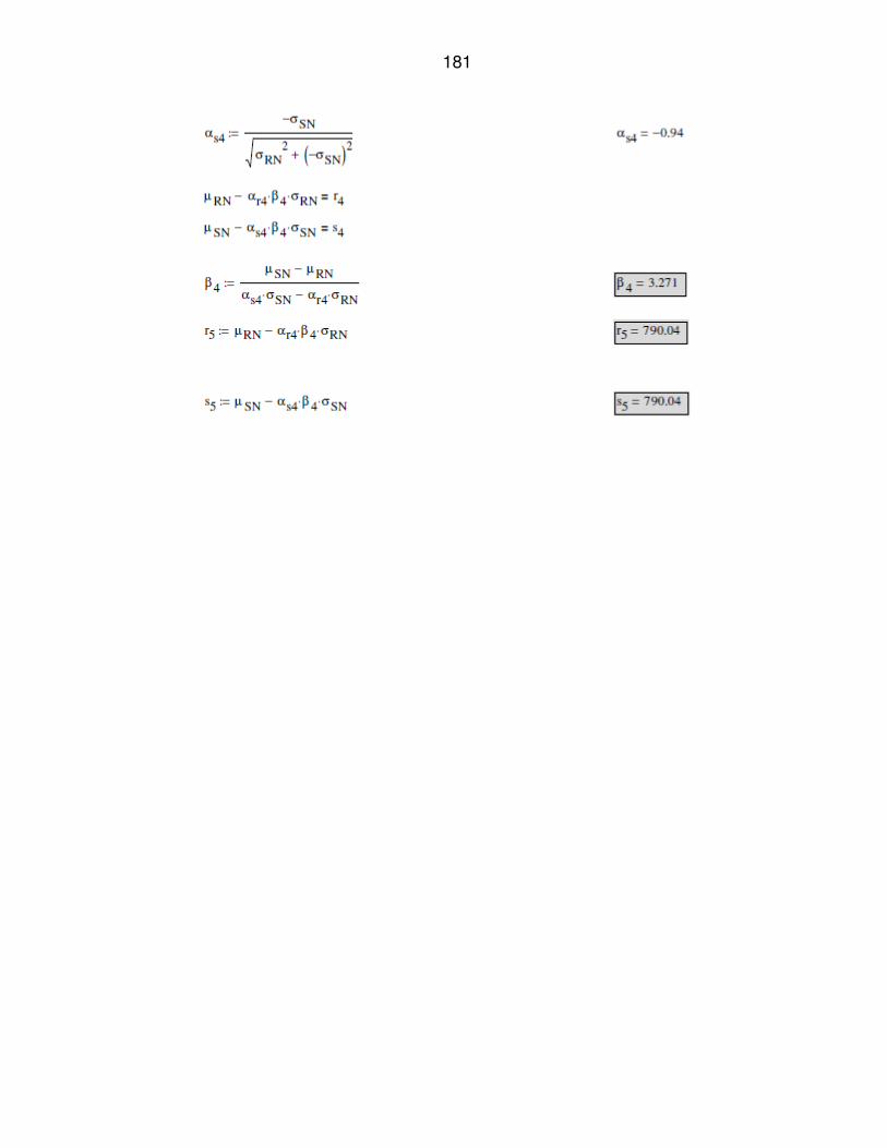
181
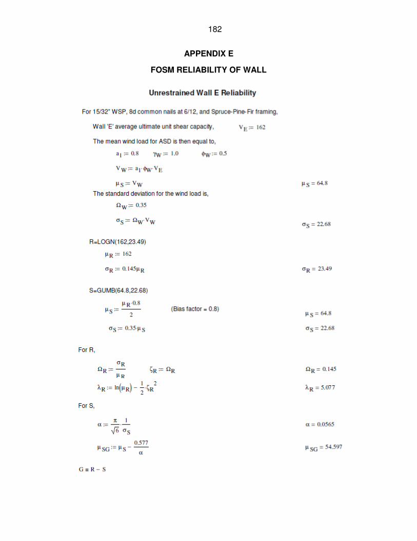
182
APPENDIX E
FOSM RELIABILITY OF WALL

183

184

185

186

187

APPENDIX F
MONTE CARLO SIMULATION
18
8

189
APPENDIX G
EXAMPLE CALCULATIONS OF UNIT SHEAR
This appendix illustrates the use of the proposed partial restraint factor. Also, a
comparison of both ASD and LRFD methods are provided as examples and
comparison.
Examples of Proposed Design Method-
Consider a wall partially restrained with a dead load. The following design information
is provided. What is the wall unit shear capacity?
Given: P=2,000 lb H=8’ L=4’ SPF-S Framing Members, G=0.36 15/32” OSB Sheathing 8d Common nails with 6:12 nail pattern ½” Anchor bolt 12” from leading edge
ASD- Solution-
From SDPWS (2005), Table A.4.3A, plf 628360501730 =−−×= ))..((Vn
Load Combination 1: D+W
plf 2012
6390628
639019903980309139805090
39808628
2000
2
==
=++−=
=×
=
).('V
..).(.).(.C
.C
n
pr
p
Load Combination 2: 0.6D+W

190
Governs plf 1902
6040628
604020702390163064210
23908628
200060
09709257
←==
=++=
=×
=
−−
).('V
..)).(..(C
.)(.
C
n
..
pr
p
ASD Unit Shear Capacity is 190 plf
LRFD-
Solution-
From SDPWS (2005), Table A.4.3A, plf 628360501730 =−−×= ))..((Vn
Load Combination 1: 1.2D+1.6W
plf 22261
3550
plf 355708062880
708020304770294147804980
47808628
200021
2
==γ
φ=
==φ
=++−=
=×
=
.
.'VV
).)((.'V
..).(.).(.C
.)(.
C
n
n
pr
p
Load Combination 2: 0.9D+1.6W
ASD)as (Same Governs plf 19061
303
plf 303603062880
603020303580294135804980
35808628
200090
2
←==γ
φ=
==φ
=++−=
=×
=
.
'VV
).)((.'V
..).(.).(.C
.)(.
C
W
n
n
pr
p
LRFD Unit Shear Capacity is 190 plf (unfactored)

191
REFERENCES
ABAQUS Analysis User’s Manual V6.10. 2010. Dassault Systems. Providence, RI.
American Forest & Paper Association (AF&PA). 1991. National Design Specification
for Wood Construction Commentary. AF&PA, Washington, DC.
American Forest & Paper Association (AF&PA). 2005. Special Design Provisions for
Wind and Seismic (ANSI/AF&PA SDPWS-2005). AF&PA, Washington, DC.
American Forest & Paper Association (AF&PA). 2005. National Design Specification
for Wood Construction (ANSI/AF&PA NDS-2005). AF&PA, Washington, DC.
American Forest & Paper Association (AF&PA). 1999. General Dowel Equations for
Calculating Lateral Connection Values (Technical Report 12). AF&PA,
Washington, DC.
American Plywood Association (APA), 2004. Panel Design Specification (Form No.
D510). APA, Tacoma, Washington.
American Plywood Association (APA), 2007. Engineered Wood Construction Guide
(Form No. E30U). APA, Tacoma, Washington.
American Plywood Association (APA), 2004. Wood Structural Panel Shear Walls
(Research Report 154). APA, Tacoma, Washington.
American Plywood Association (APA), 2007. Wood Structural Panel Shear Wall
Deflection Formula (TT-053). APA, Tacoma, Washington.
American Society of Civil Engineers (ASCE). 2005. Minimum Design Loads for
Buildings and Other Structures, ASCE 7-05. ASCE, Reston, VA.
192
Barringer. 2007. Problem of The Month – March 2001 – Heat Exchanger IRIS Wall
Thickness and Gumbel Smallest Distributions. http://www.barringer1.com/
mar01prb.htm.
American Society for Testing and Materials (ASTM). 2000. “Standard Practice for
Static Load Test for Shear Resistance of Framed Walls for Buildings”. ASTM
E564-00. Philadelphia, PA
American Society for Testing and Materials (ASTM). 2005. “Standard Test Methods of
Conducting Strength Tests of Panels for Building Construction”. ASTM E72-05.
Philadelphia, PA
American Society for Testing and Materials (ASTM). 2006. “Standard Practice for
Establishing Clear Wood Strength Values”. ASTM D 2555-06. Philadelphia, PA
American Society for Testing and Materials (ASTM). 2002, “Standard Test Methods for
Specific Gravity of Wood and Wood-Based Materials,” ASTM D2395-02.
Philadelphia, PA.
Cassidy, D. 2002. “Development and Structural Testing of FRP Reinforced OSB
Panels for Disaster Resistant Construction.” Masters Thesis. The University of
Maine. Orono, ME.
Crandell, J.H. 2007. “The story behind the IRC wall bracing provisions.” Wood Design
Focus, 17(2) (Summer). Forest Products Society, Madison, WI.
Crandell, J.H. and Martin, Z. 2009. “The story behind the 2009 IRC wall bracing
provisions (Part 2: New wind bracing requirements).” Wood Design Focus, 19(1)
(Spring). Forest Products Society, Madison, WI.

193
Crandell, J.H. and Kochkin, V. 2003. “Common engineering issues in conventional
construction.” Wood Design Focus, 13(3) (Fall). Forest Products Society,
Madison, WI.
Dolan, J.D. and Foshci, R.O. 1991. “Structural Analysis Model for Static and Dynamic
Loads on Timber Shear Walls.” J. Struct. Eng., American Society of Civil
Engineers, 117(1), 851-861.
Dolan, J.D. and Madsen, B. 1992. “Monotonic and Cyclic Tests of Timber Shear
Walls.” Canadian Journal of Civil Engineering, 19(1), 97-104.
Dolan, J.D. and Heine, C. 1997. “Sequential phased displacement tests of wood-
framed shear walls with corners.” Report No. TE-1997-003. Brooks Forest
Products Research Center, VPI&SU, Blacksburg, VA.
Dolan, J.D., Gutshall, S.T., and McClain, T.E. 1995. “Monotonic and Cyclic Tests to
Determine Short-Term Load Duration Performance of Nail and Bolt
Connections.” Report No. TE-1994-001. Brooks Forest Products Research
Center, VPI&SU, Blacksburg, VA.
Ellingwood, B.R., Galambos, T.V., MacGregor, J.G., and Cornell, C.A. 1980.
“Development of a probability based load criterion for American National
Standard A58.” Special Publication SP577, U.S. Department of Commerce –
National Bureau of Standards, Washington, DC.
Ellingwood, B.R. 1999. “A comparison of general design and load requirements in
building codes in Canada, Mexico, and the United States.” Eng. J. AISC, Second
Quarter, 67-80.

194
FSC. RB148 “Improved wind bracing analysis.” http://www.foamsheathing.org/bracing
analysis.php.
Folz, B., and Filiatrault, A. 2000. “CASHEW – Version 1.0, A Computer Program for
Cyclic Analysis of Wood Shear Walls.” Report No. SSRP – 2000/10, Structural
Systems Research Project, Department of Structural Engineering, University of
California, San Diego, La Jolla, California.
Folz, B., and Filiatrault, A. 2001. “Cyclic Analysis of Wood Shear Walls.” J. Struct.
Eng., American Society of Civil Engineers, 127(4), 433-441.
HUD. 2001. Review of Structural Materials and Methods for Home Building in the
United States: 1900 to 2000. U.S. Department of Housing and Urban
Development, Washington, DC. (publication available through
www.huduser.org).
International Code Council (ICC). 2009. International Residential Code. ICC, Falls
Church, VA.
JCSS. 2001. Probabilistic Model Code (Parts I and II). Joint Committee of Structural
Safety. http://www.jcss.ethz.ch/publications/publications_pmc.html.
Judd, J. 2005. “Analytical Modeling of Wood-Frame Shear Walls and Diaphragms.”
Master’s Thesis. Brigham Young University. Provo, UT.
Mack, J.J. 1966. “The strength and stiffness of nailed joints under short duration
loading.” Technical Paper No. 40, CSIRO Division of Forest Products.
Commonwealth Scientific and Industrial Research Organization. Melbourne,
Australia.

195
Mack, J.J. 1977. “The load-displacement curve for nailed joints.” Journal of the
Institute of Wood Science. Institute of Wood Science, 7(6), 34-36.
Ni, C and Karacabeyli, E. 2000. “Effect of overturning restraint on performance of shear
walls.” Proceedings of the World Conference of Timber Engineering, 2000.
NIST/SEMATECH. 2010 e-Handbook of Statistical Methods. http://www.itl.nist.gov/
div898/handbook/.
NIST. 2004. Performance Standard for Wood-Based Structural Use Panels, DOC PS2-
04. United States Department of Commerce, National Institute of Standards and
Technology, Gaithersburg, MD.
Seaders, P. 2004. “Performance of Partially and Fully Anchored Wood Frame Shear
Walls Under Monotonic, Cyclic & Earthquake Loads.” Masters Thesis. Oregon
State University. Corvallis, OR.
Structural Building Components Research Institute (SBCRI), 2010. “IRC Wall Panel
Testing.” http://www.sbcri.info/common/kb/techIRCnotes.php.
Structural Building Components Research Institute (SBCRI), 2010. “2009 International
Residential Code (IRC) Braced Wall Panel Design Value Comparative
Equivalency Testing – Braced Wall Panel Design Values.” SBCA, Madison,
Wisconsin.
van de Lindt, J.W., and Walz, M.A. 2003. “Development and Application of Wood
Shear Wall Reliability Model.” J. Struct. Eng., American Society of Civil
Engineers, 129(3), 405-413.
van de Lindt, J.W. 2004. “Evolution of wood shear wall testing, modeling, and reliability
analysis: Bibliography.” Pract. Period. Struct. Des. Const., 9(1), 44-53.
196
van de Lindt, J.W., and Rosowsky, D.V. 2005. “Strength-based reliability of wood
shearwalls subject to wind load.” J. Struct. Eng., American Society of Civil
Engineers, 131(2), 359-363.
Waltz, N and Hamburger, R. 2008. “New Rules for Evaluating Seismic Performance of
Prefabricated Shear Panels.” Structure Magazine, August, 2008.
WBDG. 2010. Wind Safety of the Building Envelope. http://www.wbdg.org/resources/
env_wind.php?r=dd_fireprotecteng.
Zunzun.com

197
ABSTRACT
RELIABILITY AND EFFECT OF PARTIALLY RESTRAINED WOOD SHEAR WALLS
by
JOHN J. GRUBER
May 2012
Advisor: Dr. Gongkang Fu
Major: Civil Engineering
Degree: Doctor or Philosophy
The prescriptive design of the most widely used residential building code in the
United States, the IRC, allows the use of partially restrained wood shear walls to resist
wind and seismic loads. Wind load is the most common controlling lateral design load
for these structures. In contrast, the complimenting building code, the IBC, requires
either a restraining dead load or a mechanical hold down device to resist overturning.
To prescribe a safe structure, it is important to know the effect of partial restraint on the
overturning resistance of wood shear walls constructed in accordance with the IRC and
equally important whether the partially restrained wood shear walls provide the same
level of reliability as fully restrained wood shear walls for wind load. This is the focus of
this research.
Twenty five Monotonic tests were conducted of 4’ x 8’ wood shear walls with five
varying restraining methods (wall types). There were five sets of five wall types. One of
the sets had only an anchor bolt, three sets had different dead loads with one anchor
bolt, and one set had a mechanical hold down. The results of the test program were
used to determine the partial restraint effect, create a nonlinear finite element model,

198
and to determine the statistical data required to perform a Monte Carlo simulation of the
wall behavior.
The Monte Carlo simulation result was used to calibrate a nonlinear partial
restraint factor to a target reliability index of 3.25. The calibration was performed for
both ASD and LRFD load combinations as required by the IBC. The research
concludes with a closed-form solution, including the calibrated nonlinear partial restraint
factor developed, to determine the unit shear capacity of a partially restrained or fully
restrained (with dead load or mechanical hold down) wood shear wall constructed in
accordance with the IRC by utilizing the fully restrained nominal unit shear values of
AF&PA’s Special Design Provisions for Wind and Seismic.

199
AUTOBIOGRAPHICAL STATEMENT
John J. Gruber
Mr. Gruber was born in Grosse Pointe, Michigan on May 21, 1965. He received
his B.S. degree in Construction Engineering in 1991 from Lawrence Technological
University, Southfield, MI. Upon graduation from LTU, he became employed as a
structural consulting engineer at Sheppard Engineering in Troy, MI. In 2001, he and
three partners, purchased Sheppard Engineering from the owner and he has been a
partner and President of Sheppard Engineering since the purchase. He is a licensed
professional engineer in four states and a licensed structural engineering in Illinois. He
has also instructed both undergraduate and graduate courses at Wayne State
University as an adjunct professor since 2009.
Mr. Gruber resumed his college studies in 2003 at the Civil and Environmental
Engineering Department at Wayne State University where he completed his M.S.
degree in Civil Engineering in 2006. He continued studying towards his doctoral degree
since that time.
Mr. Gruber is a past and current member of the ANSI/TPI 1 project committee as
well as the ANSI/TPI 3 project committee and is a member of the SBCA Engineering &
Technology Committee. He as authored and presented the following publication:
Gruber, John J. “Permanent Bracing of Metal Plate Connected Wood Trusses,” 9th World Conference of Timber Engineering. 2006. Portland, OR, USA.
Top Related