


Languages
Pages
Legal


Regression Basics

How is Regression Different from
other Spatial Statistical Analyses?
With other tools you ask WHERE something is
happening?
Are there places in the United States where people
are persistently dying young?
Where are the hot spots for crime, 911 emergency
calls, or fires?
Where do we find a higher than expected proportion
of traffic accidents in a city?

With Regression Analyses, you ask WHY something is happening.
Why are there places in the United States where people persistently die young? What might be causing this?
Can we model the characteristics of places that experience a lot of crime, 911 calls, or fire events to help reduce these incidents?
What are the factors contributing to higher than expected traffic accidents? Are there policy implications or mitigating actions that might reduce traffic accidents across the city and/or in particular high accident areas?

Regression analysis allows you to…
Model, examine, and explore spatial
relationships
Predict
Coefficients for percent rural and
low-weight births
T-scores show where this
relationship is significant

Reasons to Use Regression Analysis
To model phenomenon in order to better
understand it and possibly make decisions
To model phenomenon to predict values at other
places or times
To explore hypotheses

Regression Models

Spatial Regression
Spatial data often do not fit traditional, non-spatial
regression requirements because they are:
spatially autocorrelated (features near each other
are more similar than those further away)
nonstationary (features behave differently based on
their location/regional variation)
No spatial regression method is effective for both
characteristics.
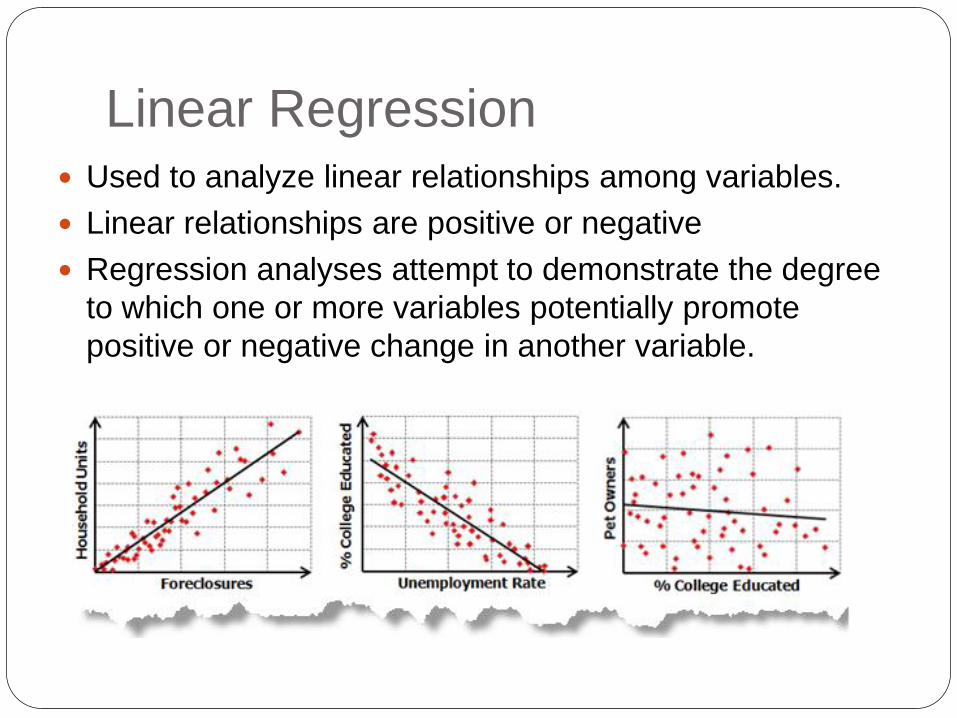
Linear Regression Used to analyze linear relationships among variables.
Linear relationships are positive or negative
Regression analyses attempt to demonstrate the degree
to which one or more variables potentially promote
positive or negative change in another variable.

Linear Regression Equation
Y = variable you are trying to predict or understand
X = value of the dependent variables
β = coefficients computed by the regression tool, represent the strength and type of relationship X has to Y
Residuals = the unexplained portion of the dependent variable large residuals = a poor model fit
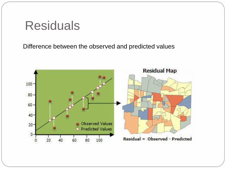
Residuals
Difference between the observed and predicted values

Ordinary Least Squares Regression
Best known technique and a good starting
point for all spatial regression analyses.
Global model = provides 1 equation to represent
the entire dataset
Available in Geoda and ArcMap

Geographically Weighted Regression
(GWR) (ArcMap)
Provides a local model of the variable by fitting a
regression equation to every feature in the
dataset.
The equations incorporate the dependent and
explanatory variables of features falling within the
bandwidth of each target feature.

Spatial Lag Model (Geoda) Includes a spatially lagged dependent variable:
y=(ρ)Wy + X(β) + ε Wy = spatially lagged dependent variable for weights
matrix W
X = matrix of observations on the explanatory variable
ε = vector of error terms
ρ and β are parameters
A spatial lag is a variable that averages the neighboring values of a location.
Accounts for autocorrelation in the model with the weights matrix y is dependent on its neighbors (through the weights
matrix)
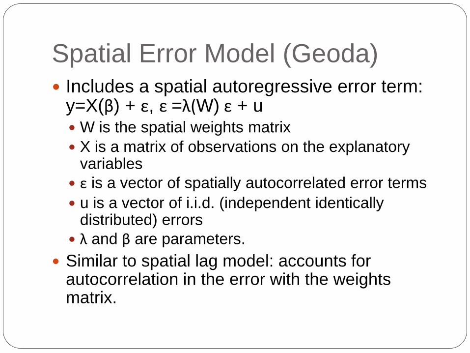
Spatial Error Model (Geoda) Includes a spatial autoregressive error term:
y=X(β) + ε, ε =λ(W) ε + u W is the spatial weights matrix
X is a matrix of observations on the explanatory variables
ε is a vector of spatially autocorrelated error terms
u is a vector of i.i.d. (independent identically distributed) errors
λ and β are parameters.
Similar to spatial lag model: accounts for autocorrelation in the error with the weights matrix.

Interpreting Results

Summary Statistics Mean/Standard Deviation
Number of observations
Dependent Variable

Measure of Regression Fit
R2
How well the regression
line fits the data
The proportion of
variability in the dataset
that is accounted for by
the regression equation.
Ranges from 0 to 1
Outliers or non-linear
data could decrease R2.

Data Outliers
Solutions:
Run regression with and
without outliers to see
their effect on the analysis
Create a scatter plot to examine extreme values and correct or remove outliers if possible.

Nonlinear Relationships
Solutions:
Create a scatter plot
matrix graph and
transform variables
Use a non-linear
regression model

Variable Coefficients
The sign shows whether the relationship is
positive or negative
The coefficient shows the strength of the
relationship.
P-values indicate whether the variable is a
significant predictor of the independent variable.
Use the coefficients to form a regression
equation: y = 10 + .5a – 6b + 8c
Remove variables with high p-values to see if R2
increases.

Comparability
Use Akaike information Criterion (AICc) value
when comparing models.
AICc is a measure of the relative goodness of fit
of a statistical model.
It assists with model selection, but does not test
the null hypothesis.
A lower AICc value means the model is a better fit
for the data.

Multicollinearity
Two or more variables may be highly correlated
with one another
Variance Inflation Factor (VIF)
Larger than 7.5 could indicate redundancy among
variables.
Multicollinearity Condition Number
Values over 30 indicate a problem

Tests for Residuals/Errors Jarque-Bera Test: Tests the normality of errors. If it is
significant, you may be missing an explanatory variable.
Breusch-Pagan, Koenker-Bassett, White: Test for heteroskedasticity (non-constant variance). If these are significant, the relationships between some or all of the explanatory variables and the dependent variable are non-stationary (a strong predictor in one area, but weak in others). Try other regression models (GWR, etc.)
Spatial Autocorrelation: Autocorrelated residuals could indicate missing variables or the need for alternative regression models.

Normal Distribution Bias
Solutions:
Jarque-Bera tests
whether residuals are
normally distributed.
Model may be
misspecified or
nonlinear.

Spatially autocorrelated residuals
Solutions:
Run the spatial
autocorrelation tool on
the residuals.
If there is significant
clustering, there could
be misspecification (a
variable is missing
from the model).

Plotting Residuals
Residuals vs. ID (or any unique identifier)
Should not display any pattern
Examine large residuals and look for systematic
relationships to improve upon the model
Residuals vs. Predicted
Detects heteroskedasticity, or unequal variances
Funnel-like patterns indicate relationships between
the residuals and predicted values

Heteroskedasticity
•If heteroskedasticity
exists, variability
differs across sub-
populations.
•Variables could be
strong predictors in
some areas, but
weak predictors in
others.

Maps
Predicted Value Map
The value of the dependent variable, based on the
regression equation
A smoothed map
Random variability, due to factors other than those
included in the model, have been smoothed out
Residual Map
Indicates systematic over or under prediction in
regions, which could be evidence of spatial
autocorrelation

Summary

Steps of Regression Determine what you are trying to predict or examine
(dependent variable)
Identify key explanatory variables
Examine the distribution to determine the type of regression to conduct
Run the regression
Examine the coefficients
Examine the residuals The mean should equal 0.
They should create a random pattern. They should create a normal distribution. Problems could indicate missing variables.
Remove or add variables and repeat regression
Use another regression model if necessary.

Resources

Regression Resources ESRI Spatial Statistics Website:
http://blogs.esri.com/Dev/blogs/geoprocessing/archive/2010/07/13/Spatial-
Statistics-Resources.aspx
Geoda Workbook:
https://geodacenter.asu.edu/system/files/geodaworkbook.pdf
ESRI Regression Tool Help:
http://resources.arcgis.com/en/help/main/10.1/index.html#/An_overview_of_the_
Modeling_Spatial_Relationships_toolset/005p0000001w000000/
Video lecture on Spatial Lag and Error:
https://geodacenter.asu.edu/spatial-lag-and

Survey
Access our workshop survey at the following site:
http://libguides.mit.edu/gisworkshops
Click on Survey in the Regression box on the left
side of the page.
Top Related