


Languages
Pages
Legal

Redistribution and Market Efficiency:
An Experimental Study
Jens Großer and
Ernesto Reuben
Redistribution and Market Efficiency:
An Experimental Study*
Jens Großer
Florida State University and Institute for Advanced Study, Princeton, e-mail: [email protected]
Ernesto Reuben
Columbia University and IZA, e-mail: [email protected]
ABSTRACT
We study the interaction between competitive markets and income redistribution that reallocates
unequal pre-tax market incomes away from the rich to the poor majority. In one setup, participants
earn their income by trading in a double auction (DA) with exogenous zero or full redistribution. In
another setup, after trading, they vote on redistributive tax policies in a majoritarian election with two
competing candidates. This results in virtually full redistribution, even when participants have the
opportunity to influence taxes by transferring money to the candidates. We find that the high
redistribution reduces trading efficiency, but not as much as predicted if market participants trade
randomly. This is because, rather than capitulating to the much lower trading incentives, many
participants respond to redistribution by asking and bidding more conservatively in the DA, and in this
way help to prevent further efficiency losses.
JEL Codes: H23, D41, D72, D73
Keywords: redistribution, double auction, market efficiency, elections, lobbying
Note: This is the authors’ version of a work that was accepted for publication in the Journal of Public Economics.
Changes resulting from the publishing process may not be reflected in this document. A final version is published
in http://dx.doi.org/10.1016/j.jpubeco.2013.02.002.
* Financial support from the GEW Foundation Cologne and the German Science Foundation (DFG) is gratefully
acknowledged. We would also like to thank the Economics Laboratory of the University of Cologne for their help
and hospitality.
1
1. Introduction
A major concern of modern democracies is to implement an optimal degree of redistribution
that reallocates income away from the well-to-do to the relatively poor. This is a delicate
balancing act between the people’s taste for equality and the potentially negative
consequences of redistribution for economic efficiency. Citizens generate wealth by
participating in a variety of different markets. Usually, this wealth is distributed unequally
(e.g., due to differences in individual productivities). However, a majority of relatively poor
citizens have, in principle, the opportunity to counteract the often dramatic inequality by
determining the degree of income redistribution in elections. In the present paper, we study
one important aspect of the balancing act between the fundamental conflict of the principles
of markets (“one dollar, one vote”) and elections (“one person, one vote”), namely, the effects
of redistribution on market trading behavior and efficiency. This is very different to the
previous literature in which redistribution influences wealth through various other channels
(e.g., Alesina and Giuliano 2009), such as the people’s labor-leisure choice (e.g., Meltzer and
Richard 1981; Romer 1975).
So far, experimental markets and (redistribution in) elections have been studied in
isolation. Many laboratory markets—in particular Smith’s (1962) double auction (henceforth
DA)—reliably clear at approximate equilibrium prices and quantities, and in this way
generate close to the maximum possible wealth, or trading efficiency (for surveys, see Davis
and Holt 1993; Kagel and Roth 1995). Similarly, median voter preferences are reflected
reliably by outcomes of laboratory two-candidate elections with compulsory majority voting
(for a survey, see McKelvey and Ordeshook 1990). While these literatures have substantially
contributed to our understanding of how markets and elections function independently, they
shed little light on how they interact and perform when they coexist. Given that trading
efficiency can be negatively affected if there are interdependencies between the earnings of
traders beyond those implied by market transactions (e.g., Dufwenberg et al. 2011; Goeree
and Zhang 2012; Rostek and Weretka 2010), it is important to ask: do lower trading
incentives due to redistributive taxation result in lower trading efficiency? And if so, does the
2
poor majority respond by reducing their tax demands in order to prevent a lower tax revenue
base?
In our experiment, citizens first earn their—unequally distributed—income in a DA. To
mimic the prevalent income inequality observed in democracies around the world, we chose
the market parameters such that, in equilibrium, the pre-tax income of a majority of citizens is
below the average. As this is the first experimental study of the effects of redistribution on
trading efficiency, we believe employing the DA is appropriate because it is the predominant
market used in laboratory studies (and is often used in actual financial and commodity
markets) and poses a challenge to our research question as we know that, without income
redistribution, it reliably generates the maximum possible wealth.
On the surface, introducing redistribution in a DA in the form of lump sum transfers
financed with linear income taxes à la Meltzer and Richard (1981) and Romer (1975) does not
change market prices and quantities. Without any redistribution, each transaction gives the
two involved traders a purely private return. By contrast, their private return is smaller with
redistribution (i.e., the untaxed share of their pre-tax income), but they and everybody else
also receive a public return (i.e., a lump sum transfer from the taxed share).1 Specifically, the
marginal trading incentive is non-negative and decreasing in the tax.2 Therefore, in
equilibrium, the maximum trading efficiency is obtained even with full redistribution.
Nevertheless, redistribution might affect trading behavior in different ways, and it is not
obvious that the effort necessary to achieve high trading efficiency can be maintained. In
particular, the lower marginal incentive to trade and bargain over prices might result in
unpredicted price volatility, transactions, and efficiency losses. For example, even in games
where variations in marginal incentives do not change equilibrium predictions, a bulk of
laboratory studies show that people do respond to such variations (e.g., Goeree and Holt
2001; McKelvey and Palfrey 1995). In the DA, this can manifest in careless pricing, which
1 Hence, transactions have a public good character because everyone gets a public return. This is different to
trading ‘common value’ goods, where only the respective traders earn money. See also Balafoutas et al. (2010),
who systematically vary private and public returns in a public goods experiment with unequal endowments.
2 We assume that a transaction’s after-tax income exceeds its costs (e.g., the cost of foregone leisure).
3
gives rise to substantial inefficient trading.3 Even more dramatic, if the most efficient traders
perceive the degree of taxation as unfair, one could imagine they abstain from market activity
altogether. Indeed, as many bargaining experiments suggest, depriving people of their fair
share of a surplus can trigger negative emotions that provoke them to destroy their pre-tax
income (Bosman and van Winden 2002; see also Camerer 2003). Therefore, it is reasonable to
conjecture that too much redistribution decreases trading efficiency. We study whether this is
the case by comparing experimental DAs with exogenous zero and full redistribution.
We also examine two setups with endogenous redistribution in which, after citizens have
earned their unequal incomes in the DA, two candidates compete via redistributive taxes in a
majoritarian election. In one of the setups, prior to policymaking, citizens also have the
opportunity to influence tax policies by transferring money to the candidates.4 Compared to
exogenous redistribution, these setups allow us to draw more general conclusions about the
interaction of markets and elections via income redistribution, because now market efficiency
and income equality are the outcome of a balancing act between the rich and the poor. First,
candidates might attempt to woo the poor majority with drastic redistribution, but if this
lowers the trading efficiency then the poor may in fact support more moderate taxes. Second,
if transfers to candidates are possible, the rich might attempt to lower their tax burden by
compensating them for taking the electoral risk of choosing low tax policies, which can in turn
trigger counteractive transfers by the poor.5 If candidates respond to money transfers, the
high concentration of pre-tax market income among the well-to-dos might work in their
advantage in the rent-seeking race (see also Karabarbounis 2011). However, as in everyday
3 See Davis and Holt (1993) and Kagel and Roth (1995) for market experiments with low marginal incentives that
are not caused by taxation.
4 As in many rent-seeking models (e.g., Tullock 1980), in our study, money transfers to the candidates are sunk
costs, i.e. are not conditional on policy choices, and cannot be used otherwise such as for campaigning (e.g.,
Campante 2007). Moreover, all pre-tax incomes are public information, which is different to signaling models of
lobbying (e.g., Ainsworth 1993; Grossman and Helpman 2001; Potters and van Winden 1992).
5 With counteractive lobbying (Austen-Smith and Wright 1994) the net effect of transfers on tax policies will
depend on the difference in overall transfers between the rich and poor.

4
politics where quid pro quo is generally banned and thus not contract-enforceable, candidates
are not bound to return any favors and the success of money transfers depends on their
willingness to reciprocate. In addition to gaining better knowledge of the influence of favors
on redistribution, the transfer levels give us valuable insights on the preferences for
redistribution in our experiment.
By keeping our laboratory democracy simple, we obviously abstract from a variety of other
phenomena related to income redistribution.6 However, for policymaking to be effective it
seems vital to understand how redistribution impacts the basic functioning of coexisting
markets and elections. Therefore, our paper can be seen as a first step towards a more basic
understanding of the interaction of the two institutions. To this end, laboratory studies are
ideal since in the field we generally cannot observe how they work together without them
being confounded by various other influences. Naturally, in experiments specific procedures
and parameters must be chosen. We want to stress, however, that our choices are nonetheless
representative of many of the incentives people face outside of the laboratory.
In the following, we discuss some of the important studies that are relevant to ours,
starting with the DA and continuing with empirical work on voting and preferences for
redistribution. In laboratory DAs prices and quantities quickly and reliably converge towards
predicted outcomes, even when participants have minimal information about overall supply
and demand. To understand this important result, trading behavior has been modeled and
experimentally tested in more detail. For example, Cason and Friedman (1996) perform a
systematic analysis of inefficiencies in experimental DAs and compare trading behavior to
various theoretical benchmarks (see also Friedman 1991; Gjerstad and Dickhaut 1998; Gode
and Sunder 1993). As benchmarks for trading behavior in the DA with income redistribution,
6 For example, we do not consider the relationship between redistributive politics and economic growth (Alesina
and Rodrik 1994; Benhabib and Rustichini 1996; Persson and Tabellini 1994), social mobility (Alesina and La
Ferrara 2005; Bénabou and Ok 2001), economic inefficiencies such as leaky buckets (Browning 2002), outside
options such as tax migration (Epple and Romer 1991), the survival of democracy (Benhabib and Przeworski
2006), and imperfect credit and insurance markets (Bénabou 2000). For extensive discussions, see Browning
(2002), Persson and Tabellini (2000), and Rosen and Gayer (2007).
5
we formulate a simple model that builds upon Gjerstad and Dickhaut’s rational traders who
form subjective beliefs about the DA environment and we run simulations with Gode and
Sunder’s zero-intelligence traders.
A growing literature investigates more thoroughly the origins of preferences for
redistribution (Alesina and Giuliano 2009). In the present paper, office-seeking candidates
have an incentive to woo the poor majority by selecting full redistribution. Of course, such
extreme policies are not observed in the field, and a variety of explanations have been offered
why median voter preferences for redistribution are more moderate. For example, Alesina
and Giuliano (2009) find that the taste for redistribution differs in personal traits (such as age,
gender, race, and socioeconomic status), social traits (such as history, culture, and ideology),
and fairness concerns (as in Fong 2001); and see also footnote 6. Moreover, in reality the rich
have other options to avoid high taxes such as migrating or indulging in leisure, which are not
available in our study and would limit the poor’s desire for maximal redistribution. In short,
our interest lies in the effects of redistribution on trading behavior and efficiency per se, and
how these effects influence the interplay between competitive markets and elections.
The laboratory studies of Durante and Putterman (2009), Esarey, Salmon, and Barrilleaux
(2012), and Tyran and Sausgruber (2006) are related to ours in that they too analyze income
redistribution derived from citizens’ choices. Their results often agree with those in
observational studies, supporting the notion that redistributive preferences revealed in
experiments are externally valid. In the first two experiments mentioned, self-interest
explains much of the redistribution observed, while the third study explores the conditions
under which fairness concerns can change voting outcomes (using poor minorities). However,
Durante and Putterman (2009) show that preferences for redistribution are sensitive to
changes in the setup: for example, there is lower support for redistribution if taxation is
associated with costs and deadweight losses and if participants earn their income in a real
effort task. In the abovementioned studies, taxes are determined either using the tax proposal
of the median voter or a randomly chosen participant. By contrast, in our experiment
endogenous redistribution is emerging from candidate competition, voting, and sometimes
6
monetary transfers. To the best of our knowledge, ours is the first study on the mutual impact
of redistribution and trading efficiency.7
2. Double auction with exogenous redistribution
2.1 The double auction
We use a standard DA (Smith 1962) with the added twist that market income can be subject
to exogenous income redistribution. We use throughout � = 1, … ,10 traders, five sellers and
five buyers, who may trade up to two units of a homogenous good at no cost. Seller � earns
�� = �� − � for selling her first unit plus ���
= ��� − �� for selling her second unit, where
�� denotes her cost of producing the �th unit and ��� denotes the price she receives for it.
Similarly, buyer � earns ���� = ��� − ��� for purchasing her �th unit, where ��� denotes her
reservation value for this unit and ��� denotes the price she pays for it. Units that are not
traded yield zero earnings. Both �� and ��� are exogenous and vary across traders and units
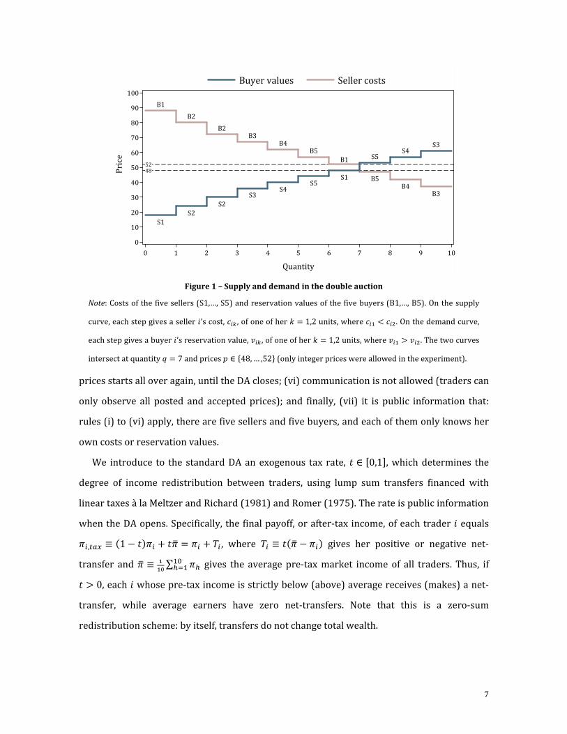
(our experimental parameters and the resulting supply and demand curves are depicted in
Figure 1). In summary, each seller’s and buyer’s pre-tax market income is given by
�� ≡ ����
+ ������ and ��
� ≡ ����� + ������
� , respectively, where ��� = 1 if she trades her
�th unit and ��� = 0 otherwise.
The following trading and information rules apply:8 (i) the DA opens for two minutes; (ii)
each seller may post an integer price ��� ∈ � �� , … , � − 1� for her �th untraded unit, where
� ≤ 100 denotes the standing seller price (i.e., the current lowest price posted by a seller or
100 if there is no posting so far) and similarly, each buyer may post ��� ∈ ��� + 1, … , ����,
where �� ≥ 0 denotes the standing buyer price (i.e., the current highest price posted by a
buyer or 0 if there is no posting so far); (iii) each seller � can accept a standing buyer price
��� = �� ≥ �� and each buyer � can accept a standing seller price ��� = � ≤ ��� (thus, pre-tax
incomes are always non-negative); (iv) each seller and buyer can trade her units one at a time,
starting with the first unit (buyers cannot resell units they have bought); (v) when a
transaction occurs, standing prices are removed and the process of posting and accepting
7 In Sausgruber and Tyran’s studies (2005, 2011), voters take into account tax shifting in markets when they vote.
8 Our procedures and parameters are similar to those used in typical laboratory DAs (see Davis and Holt 1993).
7
prices starts all over again, until the DA closes; (vi) communication is not allowed (traders can
only observe all posted and accepted prices); and finally, (vii) it is public information that:
rules (i) to (vi) apply, there are five sellers and five buyers, and each of them only knows her
own costs or reservation values.
We introduce to the standard DA an exogenous tax rate, � ∈ �0,1�, which determines the
degree of income redistribution between traders, using lump sum transfers financed with
linear taxes à la Meltzer and Richard (1981) and Romer (1975). The rate is public information
when the DA opens. Specifically, the final payoff, or after-tax income, of each trader � equals
��,� ! ≡ "1 − �#�� + ��$ = �� + %� , where %� ≡ �"�$ − ��# gives her positive or negative net-
transfer and �$ ≡ &&' ∑ �)
*)+ gives the average pre-tax market income of all traders. Thus, if
� > 0, each � whose pre-tax income is strictly below (above) average receives (makes) a net-
transfer, while average earners have zero net-transfers. Note that this is a zero-sum
redistribution scheme: by itself, transfers do not change total wealth.
Figure 1 – Supply and demand in the double auction
Note: Costs of the five sellers (S1,…, S5) and reservation values of the five buyers (B1,…, B5). On the supply
curve, each step gives a seller �’s cost, �� , of one of her � = 1,2 units, where � < ��. On the demand curve,
each step gives a buyer �’s reservation value, ���, of one of her � = 1,2 units, where �� > ���. The two curves
intersect at quantity / = 7 and prices � ∈ �48, … ,52� (only integer prices were allowed in the experiment).
B1
B2
B2B3
B4B5
B1
B5B4
B3
S1
S2
S2
S3S4
S5S1
S5S4
S3
5248
0
10
20
30
40
50
60
70
80
90
100
Pri
ce
0 1 2 3 4 5 6 7 8 9 10
Quantity
Buyer values Seller costs

8
2.2 Static and dynamic predictions
Next, we derive predictions for our DA with exogenous income redistribution, assuming that
traders are risk-neutral and maximize their own earnings. First, we conduct a static analysis
by determining equilibrium prices and quantities as the intersection of supply and demand
curves. Thereafter, we study dynamic market behavior where rational traders adjust their
minimum willingness to accept (WTA) or maximum willingness to pay (WTP) based on
subjective beliefs about how much their transaction contributes to total wealth.
Our static equilibrium prediction follows directly from Figure 1. If sellers S1 and S2 and
buyers B1 and B2 each trade their first and second units, and sellers S3, S4, and S5 and buyers
B3, B4, and B5 each trade their first units (henceforth efficient units, while all others are
inefficient units) then trading delivers the maximum possible wealth of 238 points. Thus, in
equilibrium, the average income per trader is 23.8 points and there are four ‘rich’ traders with
above-average incomes (S1, S2, B1, B2) and six ‘poor’ traders with below-average incomes
(S3, S4, S5, B3, B4, B5).9 Notably, the redistributive tax does not result in a deadweight loss
since it is calculated as a percentage of market income, which does not yield parallel inward
shifts of supply and demand curves (cf. Rosen and Gayer 2007; Ruffle 2005). This gives:
Prediction 1 (Static market equilibrium): Independent of income redistribution, any market
equilibrium is efficient and involves 7 transactions at any market price in the range [48, 52]. This
yields total wealth of 238 points, a rich minority of four traders, and a poor majority of six
traders.
In our static analysis, inefficiencies do not occur. However, since traders have minimal
information about market parameters, in a dynamic analysis rational decisions must rely on
their subjective beliefs, which give rise to inefficiencies. Compared to the benchmark of
maximum efficiency, there are two sources of trading inefficiency. First, an efficiency loss
occurs for each transaction that matches an inefficient unit with an efficient unit (e.g., seller S1
posts a price of 35 points for her first unit, and buyer B3 accepts this price for her second
9 For the median equilibrium price �∗ = 50, for example, the pre-tax incomes of the rich are 52, 46, 40, and 34
points (B2, S2, B1, and S1) while those of the poor are 17, 14, 12, 10, 7, and 6 points (B3, S3, B4, S4, B5, and S5).
9
unit). Second, an efficiency loss occurs for each efficient unit that is not traded within the
market period. Combining the two sources of inefficiency, in the one extreme where no one
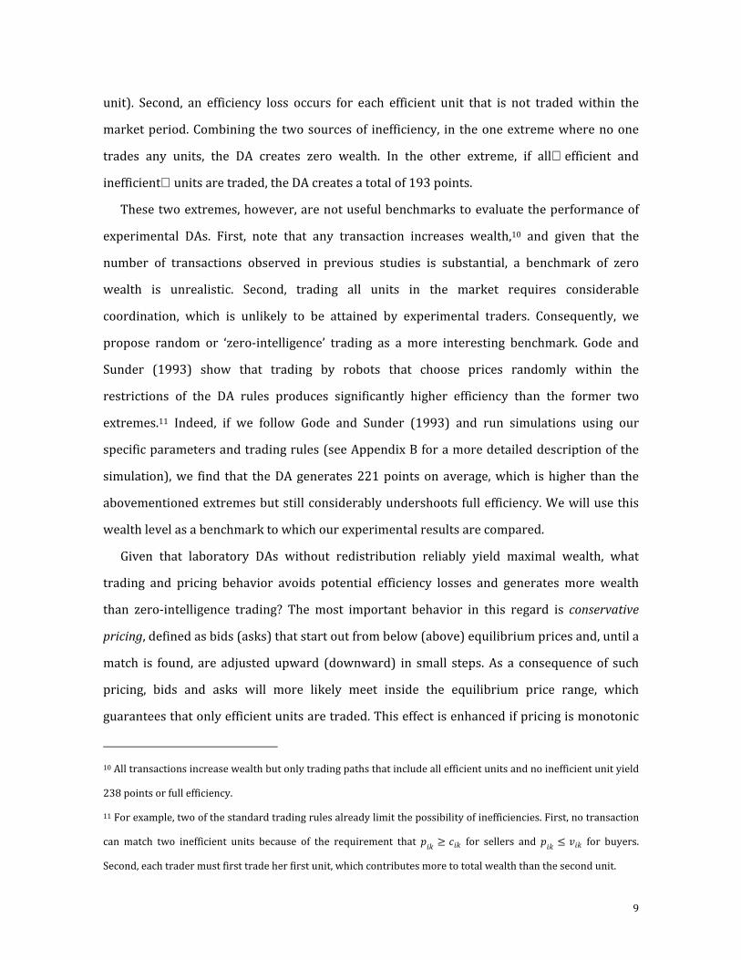
trades any units, the DA creates zero wealth. In the other extreme, if allefficient and
inefficientunits are traded, the DA creates a total of 193 points.
These two extremes, however, are not useful benchmarks to evaluate the performance of
experimental DAs. First, note that any transaction increases wealth,10 and given that the
number of transactions observed in previous studies is substantial, a benchmark of zero
wealth is unrealistic. Second, trading all units in the market requires considerable
coordination, which is unlikely to be attained by experimental traders. Consequently, we
propose random or ‘zero-intelligence’ trading as a more interesting benchmark. Gode and
Sunder (1993) show that trading by robots that choose prices randomly within the
restrictions of the DA rules produces significantly higher efficiency than the former two
extremes.11 Indeed, if we follow Gode and Sunder (1993) and run simulations using our
specific parameters and trading rules (see Appendix B for a more detailed description of the
simulation), we find that the DA generates 221 points on average, which is higher than the
abovementioned extremes but still considerably undershoots full efficiency. We will use this
wealth level as a benchmark to which our experimental results are compared.
Given that laboratory DAs without redistribution reliably yield maximal wealth, what
trading and pricing behavior avoids potential efficiency losses and generates more wealth
than zero-intelligence trading? The most important behavior in this regard is conservative
pricing, defined as bids (asks) that start out from below (above) equilibrium prices and, until a
match is found, are adjusted upward (downward) in small steps. As a consequence of such
pricing, bids and asks will more likely meet inside the equilibrium price range, which
guarantees that only efficient units are traded. This effect is enhanced if pricing is monotonic
10 All transactions increase wealth but only trading paths that include all efficient units and no inefficient unit yield
238 points or full efficiency.
11 For example, two of the standard trading rules already limit the possibility of inefficiencies. First, no transaction
can match two inefficient units because of the requirement that ��� ≥ �� for sellers and ��� ≤ ��� for buyers.
Second, each trader must first trade her first unit, which contributes more to total wealth than the second unit.

10
(i.e., posted prices of units increase with their cost and decrease with their reservation value),
in which case more efficient units are traded early and hence future transactions of inefficient
units are excluded. Finally, the opportunity to observe all posted and accepted prices allows
traders to learn how to better price their units, which speeds up equilibrium convergence in
current and future market periods. Indeed, many experiments show conservative and
monotonic pricing, frequent transactions, and rapid learning toward equilibrium prices (e.g.,
Davis and Holt 1993; Kagel and Roth 1995). Thus, we predict the same for our standard DA.
Does trading behavior in the DA change when market income is redistributed? With
respect to pricing, if � = 0, a seller’s WTA for a unit equals its costs and a buyer’s WTP for a
unit equals its reservation value. By contrast, if rational traders expect strictly positive tax
rates, � > 0, the WTA can exceed the unit’s costs and the WTP can fall below the unit’s
reservation value. In other words, in a dynamic analysis the supply and demand curves may
shift inward and pricing may be more conservative with than without redistribution. To see
the intuition of these shifts (see Appendix A for a simple model), note that each seller’s and
buyer’s after-tax income from trading consists of both a private return (i.e., the non-taxed
income share) and a public return (i.e., the lump sum transfer). In the one extreme, if � = 0, then her income is purely ‘private’, and she always wants to trade both her units, independent
of the costs or reservation values. In the other extreme, if � = 1, then her income is purely
‘public’, and it is the common goal of all traders to trade only efficient units, at any feasible
price, but not inefficient units. Importantly, when � > 0, a trader faces the following tradeoff:
selling or buying an inefficient unit increases her private returns, but this gain can be offset by
a decrease in her public returns if her transaction prevents the trade of another sufficiently
wealth-generating unit. To compensate this potential net-loss of trading, sellers (buyers)
demand a ‘premium’ by increasing their WTA (decreasing their WTP). Since the relative
importance of public versus private returns increases in the tax rate, a higher t should result
in stronger inward shifts. Moreover, if traders’ beliefs about their own costs and reservation
values compared to those of others are monotonic (i.e., preserve the rank order of actual
parameters), these shifts should be stronger for units that generate less wealth. This gives:
11
Prediction 2 (Market dynamics): For higher tax rates, sellers tend to post higher asks and
buyers tend to post lower bids. This tendency is stronger for sellers with higher costs and buyers
with lower reservation values.
2.3 Alternative predictions
There are other plausible, ‘behavioral’ predictions that are worth examining in our DA.
Specifically, we discuss the possible influence on trading of mistakes and marginal incentives.
A bulk of empirical evidence suggests that individuals are prone to make mistakes and that
marginal incentives change behavior in ways not explained by Nash equilibrium.
A useful framework that links a player’s marginal incentives and decision-making errors is
quantal response equilibrium (QRE; McKelvey and Palfrey 1995, 1998), which models
decision-making as a systematic stochastic best response where more payoff-reducing
decisions are made less often than less harmful ones. In the one extreme, when the stochastic
component is negligible, traders make no mistakes and we conjecture that Predictions 1 and 2
hold. In the other extreme, they trade randomly and we get the zero-intelligence benchmark.
Note that each �’s marginal after-tax income from trading a unit, 5��,� ! 5��⁄ = 1 − � × 89&8 , is
decreasing in the tax rate, where : denotes the number of traders, � × 89&8 gives the marginal
taxed share consisting of all equal lump sum transfers to the other : − 1 traders, and �/:
gives the marginal share returned to herself (e.g., in the two extremes, 1 if � = 0 and 1/: if
� = 1). In other words, increasing the tax rate decreases the marginal income of a transaction
and, thus, decreases the difference in after-tax incomes of trading at different prices. As a
consequence, traders make more mistakes in following a conservative pricing strategy.
Therefore, we predict that higher tax rates cause higher variance in prices, which in turn
increases the probability of transactions involving inefficient units and lower overall wealth
(as in the zero-intelligence benchmark). However, because of the element of rationality in
QRE, an interesting tradeoff arises: increasing the tax rate results in more conservative
pricing, which enhances efficiency (see Prediction 2), but this effect is countervailed by the
higher variance in prices, which reduces efficiency. We elaborate on this tradeoff in more
detail below, when discussing our experimental results.

12
2.4 Experimental design
The computerized experiment was run at the Economics Laboratory of the University of
Cologne.12 In total, 40 students participated in two sessions that lasted two hours. Earnings
were expressed in points and exchanged for cash for €1 per 17 points. Participants earned an
average of €27.00, which included a show-up fee of €2.50.
In each session, the 20 participants were randomly divided into two groups of 10 traders,
giving us 4 independent groups. There was no interaction between participants in different
groups, and this was public information. We employed two treatments with exogenous tax
rates � = 0 and � = 1 (Market-0 and Market-1). In a within-subjects design, participants
played 10 periods of Market-0 and 10 periods of Market-1, and vice versa to control for order
effects. In each period, the market was open for 2 minutes.13 At the beginning of each session,
participants were informed that there will be two parts but were not given the instructions
for the second part until the first part was completed.
At the beginning of each session, participants were randomly assigned the roles of sellers
and buyers and the costs and reservation values of their two units of the good (see Figure 1).
None of these assignments changed during the entire session, and participants were informed
about this. The instructions are available in the online appendix.
3. Results with exogenous redistribution
3.1 Market efficiency
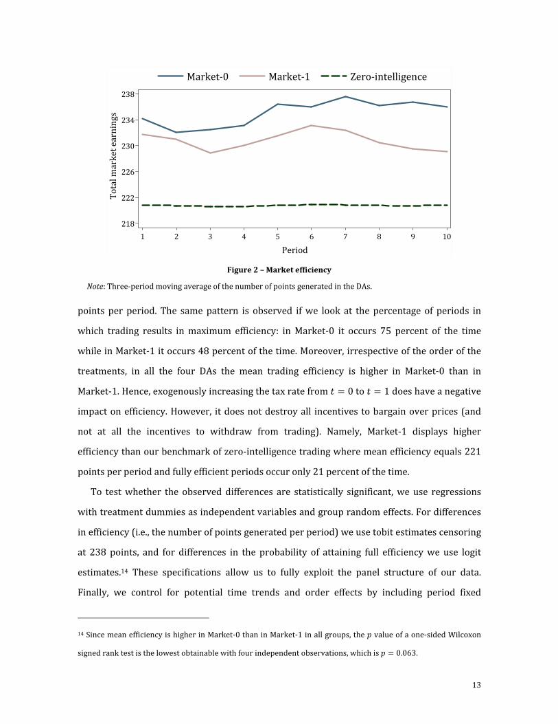
Market efficiency in each treatment and in the simulation with zero-intelligence traders is
depicted in Figure 2 (descriptive statistics are found in Appendix C). Specifically, the figure
shows the three-period moving average of the number of points generated in the DA. Recall
that maximum efficiency is reached at 238 points. As we can see, trading efficiency tends to be
higher in Market-0 compared to Market-1, particularly in the latter periods. In Market-0
trading generates an average of 235 points per period whereas in Market-1 it generates 231
12 We used z-Tree (Fischbacher 2007) for programming and ORSEE (Greiner 2004) for recruiting participants.
13 To familiarize participants with the trading rules and software, we ran three unpaid DAs before the first part.
13
points per period. The same pattern is observed if we look at the percentage of periods in
which trading results in maximum efficiency: in Market-0 it occurs 75 percent of the time
while in Market-1 it occurs 48 percent of the time. Moreover, irrespective of the order of the
treatments, in all the four DAs the mean trading efficiency is higher in Market-0 than in
Market-1. Hence, exogenously increasing the tax rate from � = 0 to � = 1 does have a negative
impact on efficiency. However, it does not destroy all incentives to bargain over prices (and
not at all the incentives to withdraw from trading). Namely, Market-1 displays higher
efficiency than our benchmark of zero-intelligence trading where mean efficiency equals 221
points per period and fully efficient periods occur only 21 percent of the time.
To test whether the observed differences are statistically significant, we use regressions
with treatment dummies as independent variables and group random effects. For differences
in efficiency (i.e., the number of points generated per period) we use tobit estimates censoring
at 238 points, and for differences in the probability of attaining full efficiency we use logit
estimates.14 These specifications allow us to fully exploit the panel structure of our data.
Finally, we control for potential time trends and order effects by including period fixed
14 Since mean efficiency is higher in Market-0 than in Market-1 in all groups, the � value of a one-sided Wilcoxon
signed rank test is the lowest obtainable with four independent observations, which is � = 0.063.
Figure 2 – Market efficiency
Note: Three-period moving average of the number of points generated in the DAs.
218
222
226
230
234
238
To
tal
ma
rke
t e
arn
ing
s
1 2 3 4 5 6 7 8 9 10
Period
Market-0 Market-1 Zero-intelligence

14
effects.15 We find that Market-0 generates significantly higher efficiency than Market-1
(� = 0.002) and attains full efficiency significantly more often (� = 0.009). Moreover, both
treatments deliver significantly higher efficiency and attain full efficiency significantly more
often than markets with zero-intelligence traders (� < 0.001). This gives:
Experimental result 1 (Efficiency): Redistribution lowers trading efficiency. However, even
with full redistribution, efficiency is higher than in simulations with traders who randomly post
and accept prices.
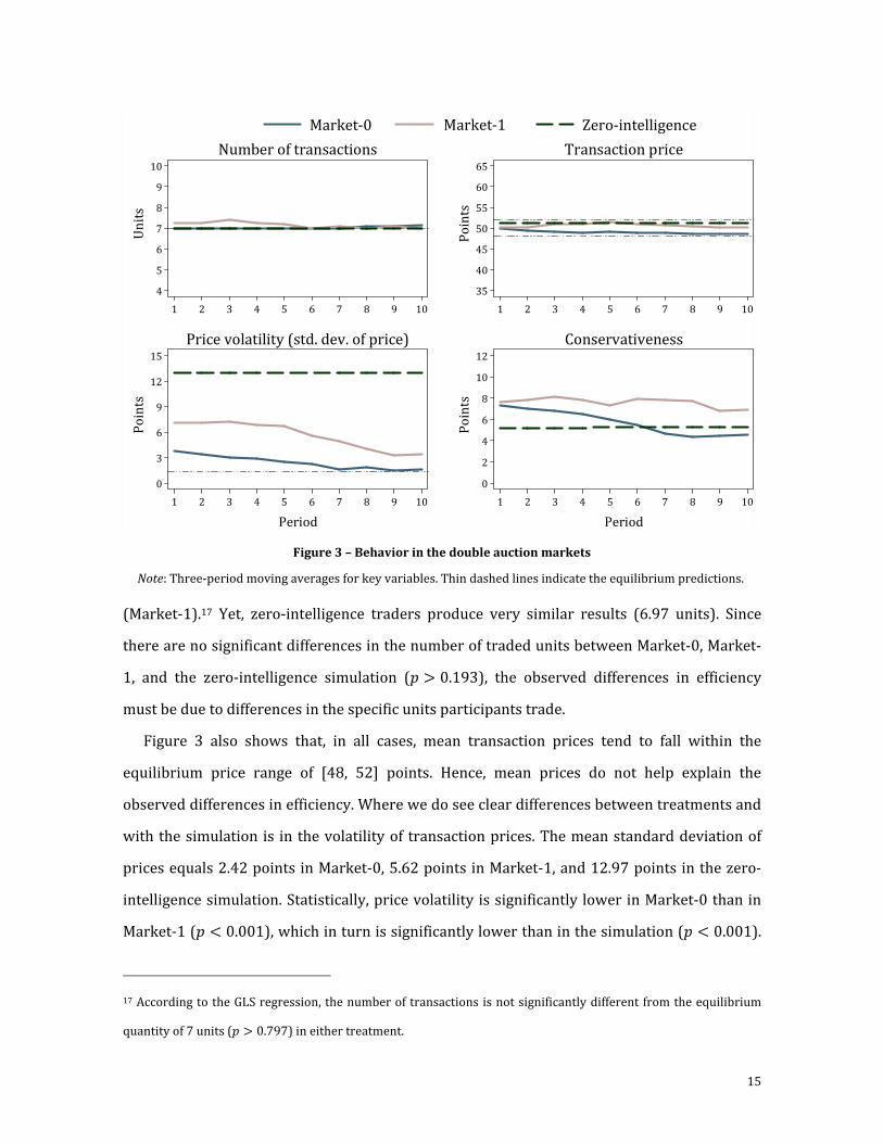
3.2 Market behavior
We further analyze market outcomes by looking at the number of transactions, transaction
prices, price volatility, and the conservativeness of bids and asks. We measure price volatility
as the standard deviation of transaction prices (calculated within each group and period). To
operationalize conservative pricing, we construct a variable that classifies bids as more
conservative the lower they are and asks as more conservative the higher they are.
Specifically, we define the conservativeness of a bid as 50 points minus the bid and that of an
ask as the ask minus 50 points. We chose 50 points as it is the middle of the equilibrium price
range [48, 52]. Figure 3 depicts the three-period moving average of these four variables. In
addition, the thin dashed lines show our equilibrium predictions (i.e., 7 transactions, prices
between 48 and 52 points, and for price volatility a standard deviation of 1.41 points derived
by uniformly randomizing between equilibrium prices). Additional descriptive statistics are
found in Appendix C. In what follows, we test whether there are statistically significant
differences using the coefficients of treatment dummy variables in GLS regressions. For each
variable, we use group means per period as the unit of observation, group random effects, and
period fixed effects.16
In both treatments, the number of transactions is consistently close to the static market
equilibrium described in Prediction 1: on average, 7.03 (7.15) units per period in Market-0
15 We also run GLS regressions with group fixed effects. Our results are the same with this specification. The output
of all regressions is available in the online appendix.
16 The online appendix contains the output of these regressions and other specifications (e.g., with fixed effects).
15
(Market-1).17 Yet, zero-intelligence traders produce very similar results (6.97 units). Since
there are no significant differences in the number of traded units between Market-0, Market-
1, and the zero-intelligence simulation (� > 0.193), the observed differences in efficiency
must be due to differences in the specific units participants trade.
Figure 3 also shows that, in all cases, mean transaction prices tend to fall within the
equilibrium price range of [48, 52] points. Hence, mean prices do not help explain the
observed differences in efficiency. Where we do see clear differences between treatments and
with the simulation is in the volatility of transaction prices. The mean standard deviation of
prices equals 2.42 points in Market-0, 5.62 points in Market-1, and 12.97 points in the zero-
intelligence simulation. Statistically, price volatility is significantly lower in Market-0 than in
Market-1 (� < 0.001), which in turn is significantly lower than in the simulation (� < 0.001).
17 According to the GLS regression, the number of transactions is not significantly different from the equilibrium
quantity of 7 units (� > 0.797) in either treatment.
Figure 3 – Behavior in the double auction markets
Note: Three-period moving averages for key variables. Thin dashed lines indicate the equilibrium predictions.
Market-0 Zero-intelligenceMarket-1
4
5
6
7
8
9
10
Un
its
1 2 3 4 5 6 7 8 9 10
Number of transactions
35
40
45
50
55
60
65
Po
ints
1 2 3 4 5 6 7 8 9 10
Transaction price
0
3
6
9
12
15
Po
ints
1 2 3 4 5 6 7 8 9 10
Period
Price volatility (std. dev. of price)
0
2
4
6
8
10
12
Po
ints
1 2 3 4 5 6 7 8 9 10
Period
Conservativeness
16
Consequently, the number of transactions that occur in the equilibrium price range differs
between Market-0 (70 percent), Market-1 (55 percent), and the simulation (17 percent); all
differences are statistically significant, � < 0.001. Given that inefficient units can be traded
only at prices outside the equilibrium price range, the higher percentage of transactions
outside this range in Market-1 and the zero-intelligence simulation explains why efficiency is
lower in these cases compared to Market-0.
Differences in transaction price volatility are consistent with the simple intuition that with
redistribution participants trade more carelessly, just not to the point where they are trading
randomly. This intuition, however, fails to explain the differences in conservative pricing. In
Market-1 we observe a mean conservativeness of 7.58 points, which is significantly higher
than in Market-0, where it equals 5.69 points (� < 0.001). Hence, consistent with Prediction 2,
participants trade more conservatively when � = 1 than when � = 0. What is interesting is
that conservativeness in the zero-intelligence simulation equals 5.23 points, which is similar
to the one in Market-0 (� = 0.161) and significantly smaller than the one in Market-1
(� < 0.001). This suggests that the higher conservativeness in Market-1 is not due to random
posting of prices, but to a systematic change in trading behavior. Overall, the observed
tradeoff between higher price volatility, which reduces efficiency, and more conservative
pricing, which enhances efficiency, is predicted by QRE (see subsection 2.3).18
We further analyze conservative pricing. According to Prediction 2, we should observe
more conservative pricing in Market-1 compared to Market-0, and this effect should be driven
by participants who hold inefficient units (i.e., asks of high-cost units and bids for low-value
units). We run three GLS regressions with conservativeness as the dependent variable. In our
first regression, the only independent variable is a treatment dummy. In our second
regression, we interact the treatment dummy with a variable measuring the expected
efficiency of the respective unit, which we operationalize as its reservation value minus 50
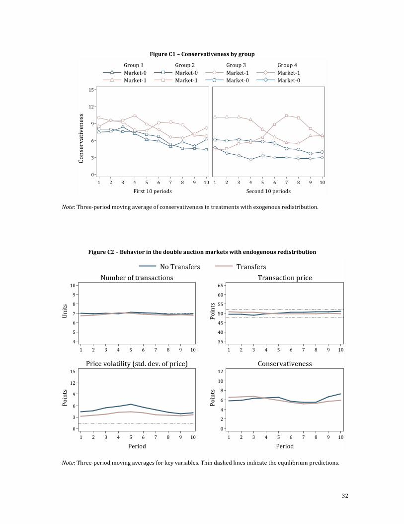
18 Since the mean conservativeness is higher in Market-1 than in Market-0 in all groups, the � value of a one-sided
Wilcoxon signed rank test is the lowest obtainable with four independent observations, which is � = 0.063. See
also Figure C1 in the appendix, which shows that, irrespective of order, groups display consistently more
conservative pricing in Market-1 than in Market-0.

17
points for buyers and 50 points minus its production cost for sellers. Finally, in the third
regression, we interact all variables with a dummy variable indicating whether a trader is a
buyer or a seller. In all regressions, we allow each participant to have an independent level of
conservativeness for each of her units, which we model as a random effect. Finally, we also
include period fixed effects.19 The regression results are shown in Table 1.
In all cases, the Market-1 dummy variable is statistically significant (� < 0.001), which
confirms that trading is more conservative when there is redistribution. Regression II shows a
negative relationship between unit efficiency and conservativeness and, more interestingly, a
significantly negative interaction term. Hence, with redistribution, participants are less
conservative when trading highly efficient units and more conservative when trading
inefficient units, as argued in Prediction 2. Once we separate buyers from sellers in Regression
III, we see that all traders are more conservative in Market-1 than in Market-0 but the
interaction with efficiency is driven by the behavior of buyers. This gives:
19 Specifically, the structure of the regression equations is: @AB��C! = D + EF��C! + GC + H�� + I��C! , where @AB��C!
is the conservativeness of trader �’s Jth bid/ask for her �th unit in period K; D is the constant; EF��C! are the vectors
of independent variables/coefficients; GC are period fixed effects; H�� are the participant and unit random effects;
and I��C! is the error term. In the online appendix, we show that our results are robust to other specifications.
Table 1 – Determinants of conservative pricing
Regression I Regression II Regression III
coef. std. err. coef. std. err. coef. std. err.
Market-1 1.72** (0.24) 2.60** (0.34) 3.09** (0.48)
Unit efficiency –0.13** (0.04) –0.09 (0.06)
Market-1 × unit efficiency –0.07** (0.02) –0.13** (0.02)
Seller –1.19 (1.52)
Seller × Market-1 –1.23 (0.69)
Seller × unit efficiency –0.11 (0.09)
Seller × Market-1 × unit efficiency 0.15** (0.04)
Constant 5.77** (0.85) 6.91** (0.93) 7.63** (1.20)
L� test for all variables 49.96** 80.79** 101.49**
Number of observations 3173 3173 3173
Number of participants 78 78 78
Note: * and ** indicate statistical significance at the 5 percent and 1 percent level.
18
Experimental result 2 (Market behavior): Mean market behavior is quite similar in markets
with and without redistribution. However, with redistribution, transaction price volatility is
higher and participants trade more conservatively.
4. Endogenous redistribution
Here, we analyze endogenous income redistribution that is determined in a majoritarian
election with two competing candidates after trading in the DA.20 In one setup, citizens have
the opportunity to influence tax policies by making monetary transfers to candidates. Hence, a
group consists of two candidates, M = N, O, and ten citizens, � = 1, … ,10, who trade in the DA
and vote in an election.21 Compared to exogenous redistribution, this allows us to examine,
more generally, the mutual influences of income redistribution and market efficiency.
4.1 Endogenous redistribution and transfers to candidates
The game with endogenous redistribution and without money transfers has three stages: a
market stage, followed by tax competition and election stages. In the market stage, citizens
earn their pre-tax income in a DA like the one in subsection 2.1. However, redistribution is no
longer exogenous and instead the tax rate � is endogenously determined in the next two
stages, which is public information when the DA opens. At the start of the tax competition
stage, the entire group is informed of all pre-tax market incomes. Thereafter, independently
and simultaneously, the two candidates choose and announce binding tax rates, �P ∈ �0,1�. In
the election stage, a majoritarian election is held (with random tie breaking) where all citizens
independently and simultaneously vote for either candidate (voting is costless and
compulsory). The winner, w, earns QR = 25 points and her tax rate, �R , determines the level of
20 There are many situations where traders must anticipate future changes in tax rates because they affect the
profitability of current trades (e.g., when buying assets whose taxable dividends are consumed over time). In our
experiment, tax uncertainty appears to have little impact, perhaps because of the low variance in the winning tax
rate. See Durante and Putterman (2009) for a study on preferences for redistribution before and after incomes are
earned.
21 For simplicity, candidates do not trade and are not subject to the tax. If they were, they could influence tax rates
in line with their own pre-tax income, which is not the focus of this paper.
19
income redistribution between citizens, whose after-tax incomes equal ��,� ! ≡ �� + %� (as in
subsection 2.1). The loser, −S ≠ S, earns QUR = 15 points and her tax rate is inconsequential.
The game with endogenous redistribution and money transfers is identical to the game just
described except that a transfers stage is added between the market and tax competition
stages. In this stage, all citizens have the opportunity to transfer points to the candidates.
Specifically, they independently and simultaneously submit a pair of transfers "V�→X, V�→Y#, where V�→P denotes the points sent by citizen � to candidate M and V� ≡ V�→X + V�→Y denotes �’s
total points sent (V� cannot exceed �’s pre-tax income, V� ∈ �0, ���). Importantly, transfers do
not change the players’ subsequent decision space. In particular, candidates are not obliged to
change their tax rates in response to transfers. Each citizen �’s final payoff is ��,� !,�Z [\]Z ≡�� + %� − V� , implying that transfers are not tax deductible, and each candidate M earns
QP,�Z [\]Z ≡ QP + P̂ , where P̂ ≡ ∑ V�→P*�+ denotes the sum of transfers M receives from all i.
4.2 Predictions
Suppose Prediction 1 holds—in particular, that there is a rich minority and a poor majority
prior to taxation. Then, we can derive predictions for the subsequent stages. We use iterated
elimination of weakly dominated strategies. Moreover, we assume that players are risk-
neutral and maximize their own earnings, and indifferent citizens vote randomly with equal
probability for each candidate. Without the transfers stage, the game’s unique subgame
perfect equilibrium is derived as follows. In the election stage, each citizen � votes sincerely
for her preferred candidate: if �P < �UP , the four rich (six poor) citizens vote for M (– M) and if
�P = �UP , they all vote randomly. This is because voting sincerely gives � a higher expected
payoff than voting insincerely when she is pivotal and her payoff is independent of her vote in
non-pivotal cases. Anticipating equilibrium voting, in the tax competition stage, candidates
choose �X∗ = �Y
∗ = 1, which weakly dominates any lower tax rate �Pa < 1, because �P
a gives M the
same payoff as �P∗ if �UP < �P
a and a lower (expected) payoff than �P∗ if �UP > "=# �P
a. With the
transfers stage, the unique equilibrium is modified as follows: citizens anticipate the decisions
described above, which are independent of any transfers, and since positive transfers only
decreases a citizen’s payoff, they all choose V�∗ = 0. This gives:
20
Prediction 3 (Endogenous income redistribution): In the tax competition and election stages,
both candidates choose full redistribution and all citizens randomize their vote between the two
candidates. The same holds when there is a transfers stage, in which case no citizen transfers any
money to the candidates.
Next, we briefly discuss political quid pro quo, which can lead to citizens making positive
transfers and candidates choosing tax rates below onein particular, the possibility that the
rich use their superior income to collude with the candidates on low taxes (at the expense of
the poor majority) by making substantial monetary transfers. Political quid pro quo of this
kind can occur if players expect mutual reciprocation (e.g., Dufwenberg and Kirchsteiger
2004; Falk and Fischbacher 2006) and has been shown to arise when one rich citizen, but not
the poor citizens, can make transfers (Großer, Reuben, and Tymula, forthcoming). However, in
our setup there are more obstacles to collusion, to wit, larger free rider and coordination
problems because more rich citizens can transfer money and the opportunity of the poor to
counteract the rich’s transfers (Austen-Smith and Wright 1994).
4.3 Experimental design
These experimental sessions used the same procedures and parameters as the ones with
exogenous redistribution (subsection 2.4). In total, 96 participants in four sessions were
randomly divided into groups of 12, each with 2 candidates and 10 citizens. Thus, we have 8
independent groups. We employed two treatments: No Transfers and Transfers, which
correspond to the DA with endogenous redistribution without and with a transfers stage (see
subsection 4.1). Participants played 10 periods of No Transfers and 10 periods of Transfers
(we reversed the sequence of both treatments across sessions). The randomly assigned roles
of sellers, buyers, and candidates did not change during the entire session.
5. Results with endogenous redistribution
In this section, we analyze behavior in No Transfers and Transfers. We provide descriptive
statistics for both treatments in Appendix C.

21
5.1 Elections and transfers
Figure 4 shows, for No Transfers and Transfers, the chosen tax rates in each period weighted
by their relative frequency (circles), the three-period moving average of the winning and
losing tax rates (lines), and the fraction of ‘insincere’ votes against ones pecuniary interest
(bars). By and large, behavior in the tax competition and election stages is consistent with
Prediction 3. Overall, in both treatments, only 3 percent of all votes are insincere22 and the
modal tax rate is � = 1 (it occurs 66 percent of the time in No Transfers and 68 percent of the
time in Transfers). Because there is a poor majority in more than 97 percent of all periods,
� = 1 is by far the most common electoral outcome in both treatments (it occurs 80 percent of
the time in No Transfers and 84 percent of the time in Transfers). The same pattern is seen for
mean (winning) tax rates, which are 0.84 (0.90) in No Transfers and 0.87 (0.95) in Transfers.
Figure 5 summarizes the citizens’ behavior in the transfers stage and the candidates’
reaction to receiving transfers. The left panel shows the three-period moving average for the
number of points each candidate receives, distinguishing between transfers from the rich and
22 Insincere voting is slightly more common among the rich than the poor (5 percent versus 2 percent).
Figure 4 – Behavior in the tax competition and election stages
Note: Chosen tax rates weighted by their relative frequency (circles), three-period moving average for
winning and losing tax rates (lines), and the fraction of insincere votes (bars).
0.0
0.2
0.4
0.6
0.8
1.0
1 2 3 4 5 6 7 8 9 10 1 2 3 4 5 6 7 8 9 10
No Transfers Transfers
Mean winning tax rate Mean losing tax rate
Chosen tax rates Fraction of insincere votesT
ax
ra
te /
fra
ctio
n o
f v
ote
s
Period
22
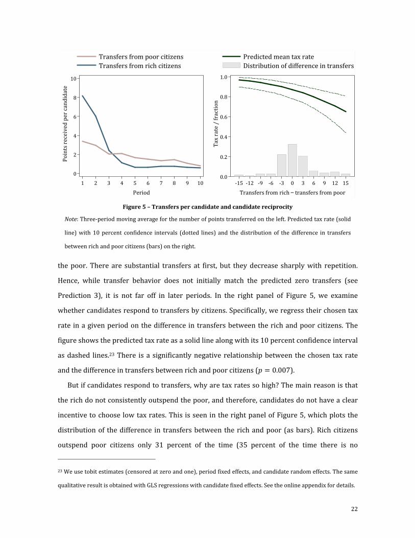
the poor. There are substantial transfers at first, but they decrease sharply with repetition.
Hence, while transfer behavior does not initially match the predicted zero transfers (see
Prediction 3), it is not far off in later periods. In the right panel of Figure 5, we examine
whether candidates respond to transfers by citizens. Specifically, we regress their chosen tax
rate in a given period on the difference in transfers between the rich and poor citizens. The
figure shows the predicted tax rate as a solid line along with its 10 percent confidence interval
as dashed lines.23 There is a significantly negative relationship between the chosen tax rate
and the difference in transfers between rich and poor citizens (� = 0.007).
But if candidates respond to transfers, why are tax rates so high? The main reason is that
the rich do not consistently outspend the poor, and therefore, candidates do not have a clear
incentive to choose low tax rates. This is seen in the right panel of Figure 5, which plots the
distribution of the difference in transfers between the rich and poor (as bars). Rich citizens
outspend poor citizens only 31 percent of the time (35 percent of the time there is no
23 We use tobit estimates (censored at zero and one), period fixed effects, and candidate random effects. The same
qualitative result is obtained with GLS regressions with candidate fixed effects. See the online appendix for details.
Figure 5 – Transfers per candidate and candidate reciprocity
Note: Three-period moving average for the number of points transferred on the left. Predicted tax rate (solid
line) with 10 percent confidence intervals (dotted lines) and the distribution of the difference in transfers
between rich and poor citizens (bars) on the right.
0
2
4
6
8
10
Po
ints
re
ceiv
ed
pe
r ca
nd
ida
te
1 2 3 4 5 6 7 8 9 10
Period
Transfers from poor citizens
Transfers from rich citizens
0.0
0.2
0.4
0.6
0.8
1.0
Ta
x r
ate
/ f
ract
ion
-15 -12 -9 -6 -3 0 3 6 9 12 15
Transfers from rich − transfers from poor
Predicted mean tax rate
Distribution of difference in transfers

23
difference and 34 percent of the time the poor outspend the rich).24 Moreover, there are even
fewer instances where both candidates receive more points from the rich than from the poor
(only 16 percent of the time), which complicates coordination among candidates (49 percent
of tax rates are lower than one but only 15 percent occur in the same period).25 Hence, poor
citizens are relatively successful in counteracting the transfers of the rich. This gives:
Experimental result 3 (Endogenous redistribution): In treatments with endogenous
redistribution, mean winning tax rates are close to full redistribution and citizens almost always
vote sincerely. If given the opportunity, rich and poor citizens make substantial monetary
transfers to candidates in early periods, but thereafter only small amounts are transferred.
Candidates choose about 20 percent lower tax rates when they receive more money from the rich
than from the poor, but this does not happen often.
5.2 Market efficiency and behavior
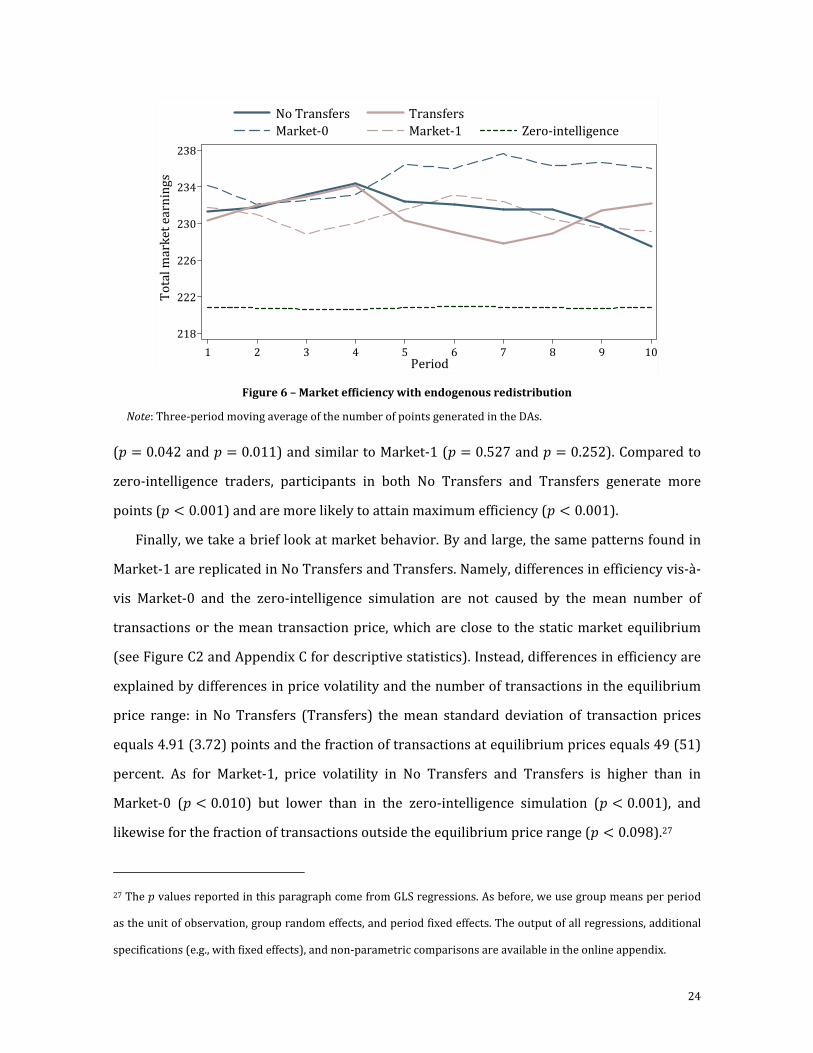
Market efficiency in No Transfers and Transfers is depicted in Figure 6 (see Appendix C for
descriptive statistics). Using electoral competition to determine tax rates yields efficiency
levels similar to those with an exogenously imposed tax rate of � = 1. On average, trading
generates 231 points per period in both No Transfers and Transfers, which is lower than in
Market-0 (� = 0.110 and � = 0.027) and comparable to that in Market-1 (� = 0.628 and
� = 0.591).26 Likewise, maximum efficiency is attained in 55 percent of all periods in No
Transfers and in 58 percent of all periods in Transfers, which is lower than in Market-0
24 If we run a GLS regression with the mean group difference in transfers between rich and poor citizens as the
dependent variable, period fixed effects, and group random effects, we find that the rich transfer significantly more
than the poor only in the first two periods (� < 0.024, otherwise � > 0.677).
25 In part, this is due to poor citizens who transfer to only one candidate 64 percent of the time, compared to rich
citizens who transfer to both candidates 61 percent of the time.
26 The � values reported in this paragraph come from regressions with group random effects and period fixed
effects. As before, we use tobit estimates (censoring at 238 points) for differences in efficiency and logit estimates
for differences in the probability of reaching full efficiency. The output of all regressions, additional specifications
(e.g., with fixed effects), and non-parametric comparisons are available in the online appendix.
24
(� = 0.042 and � = 0.011) and similar to Market-1 (� = 0.527 and � = 0.252). Compared to
zero-intelligence traders, participants in both No Transfers and Transfers generate more
points (� < 0.001) and are more likely to attain maximum efficiency (� < 0.001).
Finally, we take a brief look at market behavior. By and large, the same patterns found in
Market-1 are replicated in No Transfers and Transfers. Namely, differences in efficiency vis-à-
vis Market-0 and the zero-intelligence simulation are not caused by the mean number of
transactions or the mean transaction price, which are close to the static market equilibrium
(see Figure C2 and Appendix C for descriptive statistics). Instead, differences in efficiency are
explained by differences in price volatility and the number of transactions in the equilibrium
price range: in No Transfers (Transfers) the mean standard deviation of transaction prices
equals 4.91 (3.72) points and the fraction of transactions at equilibrium prices equals 49 (51)
percent. As for Market-1, price volatility in No Transfers and Transfers is higher than in
Market-0 (� < 0.010) but lower than in the zero-intelligence simulation (� < 0.001), and
likewise for the fraction of transactions outside the equilibrium price range (� < 0.098).27
27 The � values reported in this paragraph come from GLS regressions. As before, we use group means per period
as the unit of observation, group random effects, and period fixed effects. The output of all regressions, additional
specifications (e.g., with fixed effects), and non-parametric comparisons are available in the online appendix.
Figure 6 – Market efficiency with endogenous redistribution
Note: Three-period moving average of the number of points generated in the DAs.
218
222
226
230
234
238
To
tal
ma
rke
t e
arn
ing
s
1 2 3 4 5 6 7 8 9 10Period
No Transfers Transfers
Market-0 Market-1 Zero-intelligence
25
The only difference with exogenous redistribution is that conservative pricing in No
Transfers and Transfers is not significantly higher than in Market-0 (� > 0.667).28 Although, a
similar analysis to the one reported in Table 1 shows qualitatively similar, albeit smaller,
effects than for Market-1 (i.e., less conservative pricing by traders with more efficient units;
see the online appendix for details). This difference is possibly due to traders (correctly)
anticipating that tax rates will be somewhat lower than one. In this sense, it is suggestive that
changes in the winning tax rate, which presumably affect expectations, positively correlate
with subsequent levels of conservativeness.29 This gives:
Experimental result 4 (Market outcomes with endogenous redistribution): High levels of
redistribution chosen in competitive elections result in similar trading behavior and market
efficiency than with (imposed) full redistribution.
6. Conclusions
We experimentally study how income redistribution affects market behavior and, thus, the
generation of economic wealth. We use a double auction (DA) where, in equilibrium, market
outcomes create a rich minority and a poor majority. When we impose zero redistribution, the
DA yields nearly maximum wealth (as in many previous DAs). By contrast, in the novel setup
with exogenous full redistribution (i.e., the after-tax incomes will be the same for everyone),
wealth drops noticeably, though not as much as predicted for random trading. We attribute
the efficiency loss to lower trading incentives caused by high redistribution, which increases
the variance of asks and bids and thereby increases the number of transactions involving
inefficient units. However, interestingly, participants avoid the large efficiency loss seen with
random trading by selling and buying more conservatively with than without redistribution,
as predicted by our simple model in which rational players take into account that trading their
28 Compared to Market-1, conservativeness is significantly lower in Transfers (� = 0.003) but not in No Transfers
(� = 0.163).
29 Regressing the mean conservativeness of a group in period J on the change in that group’s winning tax rate from
period J − 2 to J − 1 (using group random effects) results in a positive and significant coefficient (� = 0.003). We
are grateful to an anonymous referee for suggesting this test.
26
own units can prevent the trade of more efficient units. To avoid a lower tax revenue base,
sellers adjust their WTA above unit costs and buyers adjust their WTP below unit reservation
values, which causes the more conservative pricing. In fact, this phenomenon should occur
more generally in markets where traders benefit directly from overall market efficiency.30
We also examine endogenous income redistribution by having citizens vote on tax policies
in a two-candidate majoritarian election. This allows us to gain insight into the mutual
influences of redistribution and market efficiency. Consistent with median voter theories, we
find that candidates woo the poor majority with very high taxes and citizens vote according to
their pecuniary self-interest. As a result, after-tax incomes are virtually equal. Moreover, the
effects we observe with exogenous full redistribution translate to behavior in the DA with
endogenous redistribution, although they are weaker since (anticipated) winning taxes are on
average somewhat smaller than one. This result does not change when, in addition to voting,
citizens can influence tax policies by transferring money to the candidates.
Our results show that the “one person, one vote” principle defeats that of “one dollar, one
vote”, but at the loss of some trading efficiency. While we focus on the DA and a two-candidate
majoritarian election, the advantage of our laboratory design is that, depending on the specific
question at hand, it can be easily extended to accommodate different markets, elections, and
ways in which they interact with each other. For example, an interesting next step could be to
provide the rich with outside options such as tax migration or leisure opportunities, which
might lower the poor’s support of income redistribution and raise trading efficiency. Other
interesting variations could be to study intermediate exogenous tax rates, rich majorities, and
costs and reservation values obtained through real effort (as in Cason, Gangadharan, and
Nikiforakis 2011). Finally, one could facilitate coordination among participants to reach
implicit or explicit agreements (as in Großer, Reuben, and Tymula, forthcoming).
Overall, our experiment can be seen as a first step to gain better knowledge of how income
redistribution influences market behavior and efficiency. More generally, it provides insights
into how the coexistence and interaction of markets and elections affect their functioning per
30 Traders can benefit directly through redistribution, as in our setup, or because they intrinsically care about
efficiency (as in Charness and Rabin 2002). See also Goeree and Zhang (2012) and Rostek and Weretka (2010).
27
se and the generation and distribution of wealth. A basic result of the present paper is that, all
else held constant, redistribution negatively impacts trading behavior and efficiency,
something that policymakers need to consider when choosing redistributive policies. For
example, even if the labor supply is inelastic and therefore increasing taxes will not markedly
reduce participation, high taxation could lead to inefficiencies because of price distortions that
are driven by noisier trading.
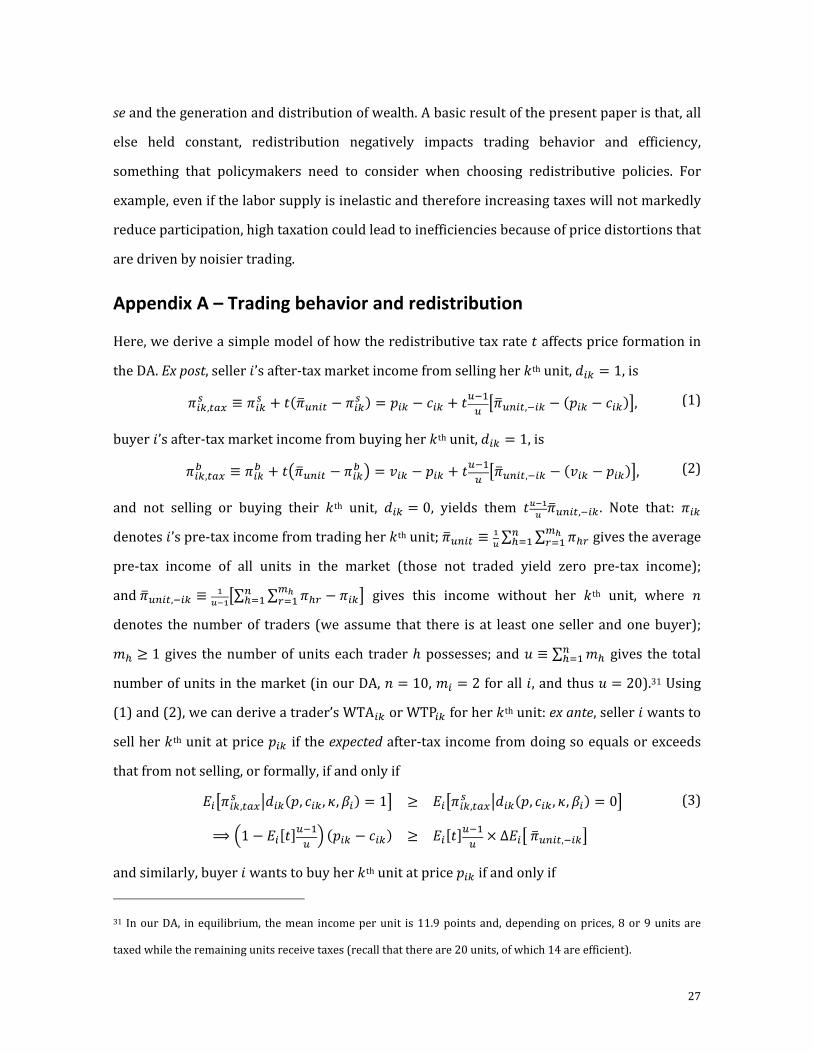
Appendix A – Trading behavior and redistribution
Here, we derive a simple model of how the redistributive tax rate � affects price formation in
the DA. Ex post, seller �’s after-tax market income from selling her �th unit, ��� = 1, is
���,� ! ≡ ���
+ �"�$b[�� − ��� # = ��� − �� + �bU
b c�$b[��,U�� − "��� − ��#d, (1)
buyer �’s after-tax market income from buying her �th unit, ��� = 1, is
���,� !� ≡ ���
� + �e�$b[�� − ���� f = ��� − ��� + �bU
b c�$b[��,U�� − "��� − ���#d, (2)
and not selling or buying their �th unit, ��� = 0, yields them �g9&g �$b[��,U�� . Note that: ���
denotes �’s pre-tax income from trading her �th unit; �$b[�� ≡ &g ∑ ∑ �)Z
hiZ+
[)+ gives the average
pre-tax income of all units in the market (those not traded yield zero pre-tax income);
and �$b[��,U�� ≡ &g9&c∑ ∑ �)Z − ���
hiZ+
[)+ d gives this income without her �th unit, where :
denotes the number of traders (we assume that there is at least one seller and one buyer);
j) ≥ 1 gives the number of units each trader ℎ possesses; and l ≡ ∑ j)[)+ gives the total
number of units in the market (in our DA, : = 10, j� = 2 for all �, and thus l = 20).31 Using
(1) and (2), we can derive a trader’s WTA�� or WTP�� for her �th unit: ex ante, seller � wants to
sell her �th unit at price ��� if the expected after-tax income from doing so equals or exceeds
that from not selling, or formally, if and only if
q�c���,� ! r���"�, �� , s, E�# = 1d ≥ q�c���,� !
r���"�, �� , s, E�# = 0d
⟹ u1 − q����bUb v "��� − ��# ≥ q����bU
b × ∆q�c �$b[��,U��d
(3)
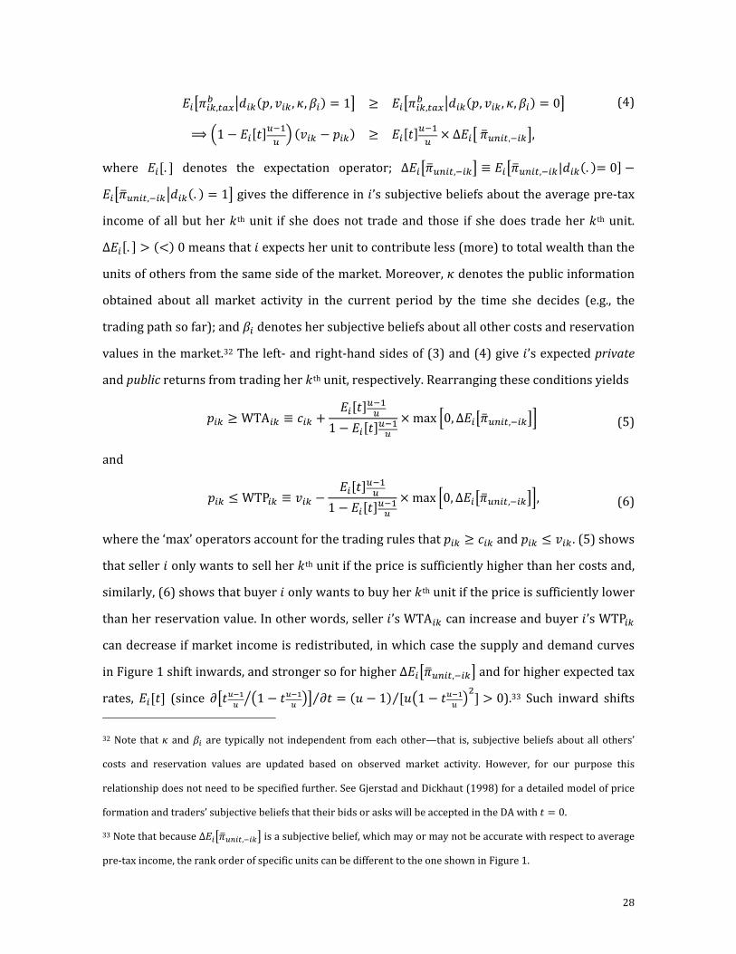
and similarly, buyer � wants to buy her �th unit at price ��� if and only if
31 In our DA, in equilibrium, the mean income per unit is 11.9 points and, depending on prices, 8 or 9 units are
taxed while the remaining units receive taxes (recall that there are 20 units, of which 14 are efficient).
28
q�c���,� !� r���"�, ��� , s, E�# = 1d ≥ q�c���,� !
� r���"�, ��� , s, E�# = 0d
⟹ u1 − q����bUb v "��� − ���# ≥ q����bU
b × ∆q�c �$b[��,U��d,
(4)
where q��. � denotes the expectation operator; ∆q�c�$b[��,U��d ≡ q�c�$b[��,U��|���". #= 0� −q�c�$b[��,U��r���". # = 1d gives the difference in �’s subjective beliefs about the average pre-tax
income of all but her �th unit if she does not trade and those if she does trade her �th unit.
∆q��. � > "<# 0 means that � expects her unit to contribute less (more) to total wealth than the
units of others from the same side of the market. Moreover, s denotes the public information
obtained about all market activity in the current period by the time she decides (e.g., the
trading path so far); and E� denotes her subjective beliefs about all other costs and reservation
values in the market.32 The left- and right-hand sides of (3) and (4) give �’s expected private
and public returns from trading her �th unit, respectively. Rearranging these conditions yields
��� ≥ WTA�� ≡ �� + q����bUb
1 − q����bUb
× max |0, ∆q�c�$b[��,U��d} (5)
and
��� ≤ WTP�� ≡ ��� − q����bUb
1 − q����bUb
× max |0, ∆q�c�$b[��,U��d}, (6)
where the ‘max’ operators account for the trading rules that ��� ≥ �� and ��� ≤ ��� . (5) shows
that seller � only wants to sell her �th unit if the price is sufficiently higher than her costs and,
similarly, (6) shows that buyer � only wants to buy her �th unit if the price is sufficiently lower
than her reservation value. In other words, seller �’s WTA�� can increase and buyer �’s WTP��
can decrease if market income is redistributed, in which case the supply and demand curves
in Figure 1 shift inwards, and stronger so for higher ∆q�c�$b[��,U��d and for higher expected tax
rates, q���� (since 5c�g9&g e1 − �g9&
g f~ d 5�⁄ = "l − 1# �le1 − �g9&g f��⁄ > 0).33 Such inward shifts
32 Note that s and E� are typically not independent from each other—that is, subjective beliefs about all others’
costs and reservation values are updated based on observed market activity. However, for our purpose this
relationship does not need to be specified further. See Gjerstad and Dickhaut (1998) for a detailed model of price
formation and traders’ subjective beliefs that their bids or asks will be accepted in the DA with � = 0.
33 Note that because ∆q�c�$b[��,U��d is a subjective belief, which may or may not be accurate with respect to average
pre-tax income, the rank order of specific units can be different to the one shown in Figure 1.
29
essentially mean that trading gets more conservative (i.e., sellers and buyers post higher and
lower prices, respectively). If their subjective beliefs about the own costs or reservation
values relative to those of other traders are monotonic (i.e., preserve the rank order of actual
costs and values) and if subjective beliefs about tax rates are not too diverse, inefficient
transactions are less likely. Moreover, if both l and q���� get large, supply and demand curve
shifts can become very large (bounded by 100 and 0) for those units that traders believe to be
inefficient (i.e., ∆q�c�$b[��,U��d > 0). Note that if it is common knowledge that both q���� = 1 for
all � and everyone knows whether her units are efficient or inefficient, then there are many
equilibria in which all efficient units are traded—at any feasible price—but no inefficient units
(this holds also for the static equilibrium analysis because it implies a unique market price).
Appendix B – Zero-intelligence traders
The simulation for zero-intelligence traders is done for the DA described in section 2 and with
the parameters seen in Figure 1. The code is available in the online appendix. Results are
based on 10,000 groups that played 10 periods each. A period follows the following sequence:
1. One trader (buyer or seller) is drawn from the group, each with equal probability.
2. If the trader is a seller, it makes an offer by drawing a number between the cost of its
current unit and the highest possible value (using a uniform distribution). If the trader is a
buyer, it makes a bid by drawing a number between the value of its current unit and the
lowest possible cost (using a uniform distribution). Draws are bounded because prices
below the lowest cost and above the highest value are never accepted.
3. If the trader is a buyer and its bid is higher than the current posted offer then the
transaction occurs (at the price of the posted offer). If its bid is lower than the current
poster offer but higher than the current posted bid then its bid becomes the new posted
bid. Lastly, if its bid is lower than the current posted bid then nothing happens. If the
trader is a seller and its offer is lower than the current posted bid then the transaction
occurs (at the price of the posted bid). If its offer is higher than the current posted bid but
lower than the current posted offer then its offer becomes the new posted offer. Lastly, if
its offer is higher than the current posted offer then nothing happens.

30
4. Steps 1 through 3 are repeated until there are no more possible transactions or up to a
maximum number of postings J. This maximum number of postings is determined at the
beginning of each period by drawing a value from the distribution F, where F is the
observed distribution of postings per period in the Market-0 treatment. The reason we
use a limit to the number of postings is that robot traders are not restricted by the two
minutes during which the market is open. In order to make the simulation as comparable
to the experiment as possible, we use the number of postings in Market-0 as representing
the effect of the time during which the market is open. The results do not vary
considerably if we change this assumption. Essentially, a smaller or larger mean of F
affects the mean number of transactions but not the other statistics.
Appendix C – Descriptive statistics
Table C1 – Market efficiency and trading behavior
Market-0 Market-1 Zero
intelligence
No
Transfers Transfers
Market efficiency
Total earnings per period 235.18 230.95 220.77 231.35 230.60
(6.11) (8.75) (19.18) (13.01) (13.96)
Percentage of periods with full
efficiency
75.00 47.50 20.65 55.00 57.50
(12.91) (17.08) (12.87) (25.63) (12.81)
Trading behavior
Number of transactions per
period
7.03 7.15 6.97 6.98 6.88
(0.36) (0.53) (0.89) (0.45) (0.49)
Percentage of periods with 7
transactions
87.50 77.50 51.18 80.00 80.00
(9.57) (17.08) (15.74) (15.12) (11.95)
Transaction price 49.04 50.58 51.17 50.16 50.08
(1.30) (2.54) (4.49) (2.93) (2.61)
Standard deviation of prices per
period
2.42 5.62 12.96 4.91 3.72
(1.62) (4.20) (3.61) (3.20) (2.18)
Percentage of prices in [48, 52]
per period
69.78 55.21 17.40 49.43 51.26
(25.95) (25.78) (13.65) (30.24) (28.49)
Conservativeness per period 5.69 7.58 5.23 6.20 5.96
(2.41) (2.34) (2.06) (3.42) (2.07)
Note: The table displays means and standard deviations in parenthesis.
31
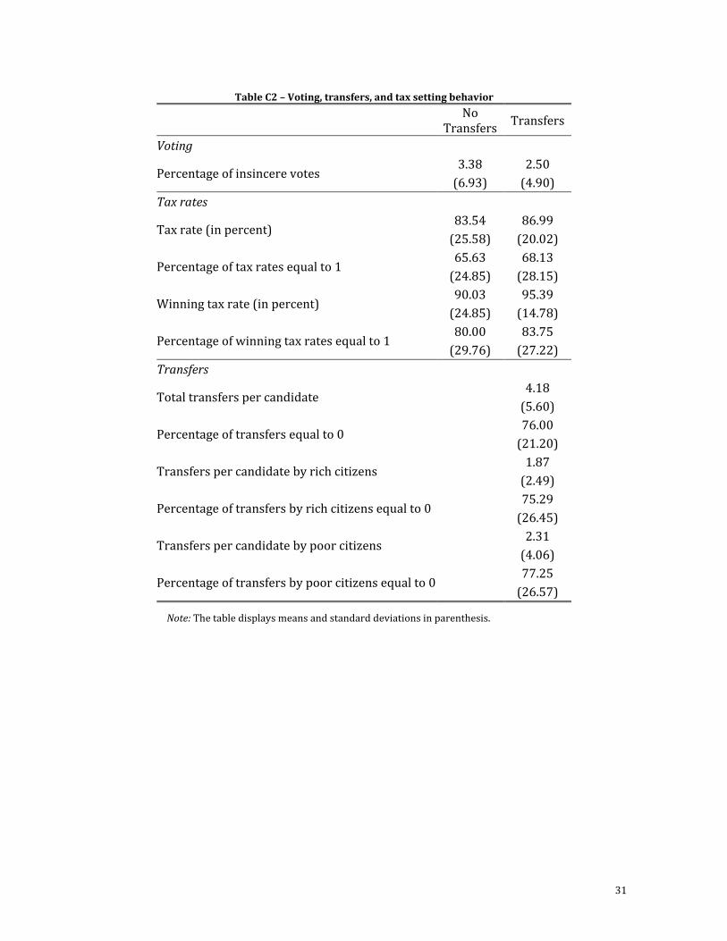
Table C2 – Voting, transfers, and tax setting behavior
No
Transfers Transfers
Voting
Percentage of insincere votes 3.38 2.50
(6.93) (4.90)
Tax rates
Tax rate (in percent) 83.54 86.99
(25.58) (20.02)
Percentage of tax rates equal to 1 65.63 68.13
(24.85) (28.15)
Winning tax rate (in percent) 90.03 95.39
(24.85) (14.78)
Percentage of winning tax rates equal to 1 80.00 83.75
(29.76) (27.22)
Transfers
Total transfers per candidate 4.18
(5.60)
Percentage of transfers equal to 0 76.00
(21.20)
Transfers per candidate by rich citizens 1.87
(2.49)
Percentage of transfers by rich citizens equal to 0 75.29
(26.45)
Transfers per candidate by poor citizens 2.31
(4.06)
Percentage of transfers by poor citizens equal to 0 77.25
(26.57)
Note: The table displays means and standard deviations in parenthesis.
32
Figure C1 – Conservativeness by group
Note: Three-period moving average of conservativeness in treatments with exogenous redistribution.
Figure C2 – Behavior in the double auction markets with endogenous redistribution
Note: Three-period moving averages for key variables. Thin dashed lines indicate the equilibrium predictions.
0
3
6
9
12
15
1 2 3 4 5 6 7 8 9 10 1 2 3 4 5 6 7 8 9 10
First 10 periods Second 10 periods
Group 1 Group 2 Group 3 Group 4
Market-0 Market-0 Market-1 Market-1
Market-1 Market-1 Market-0 Market-0C
on
serv
ati
ve
ne
ss
No Transfers Transfers
4
5
6
7
8
9
10
Un
its
1 2 3 4 5 6 7 8 9 10
Number of transactions
35
40
45
50
55
60
65
Po
ints
1 2 3 4 5 6 7 8 9 10
Transaction price
0
3
6
9
12
15
Po
ints
1 2 3 4 5 6 7 8 9 10
Period
Price volatility (std. dev. of price)
0
2
4
6
8
10
12
Po
ints
1 2 3 4 5 6 7 8 9 10
Period
Conservativeness
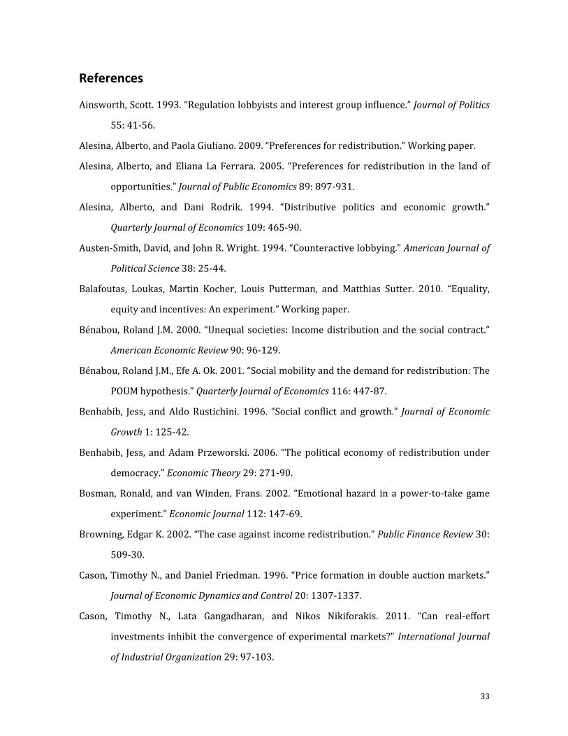
33
References
Ainsworth, Scott. 1993. “Regulation lobbyists and interest group influence.” Journal of Politics
55: 41-56.
Alesina, Alberto, and Paola Giuliano. 2009. “Preferences for redistribution.” Working paper.
Alesina, Alberto, and Eliana La Ferrara. 2005. “Preferences for redistribution in the land of
opportunities.” Journal of Public Economics 89: 897-931.
Alesina, Alberto, and Dani Rodrik. 1994. “Distributive politics and economic growth.”
Quarterly Journal of Economics 109: 465-90.
Austen-Smith, David, and John R. Wright. 1994. “Counteractive lobbying.” American Journal of
Political Science 38: 25-44.
Balafoutas, Loukas, Martin Kocher, Louis Putterman, and Matthias Sutter. 2010. “Equality,
equity and incentives: An experiment.” Working paper.
Bénabou, Roland J.M. 2000. “Unequal societies: Income distribution and the social contract.”
American Economic Review 90: 96-129.
Bénabou, Roland J.M., Efe A. Ok. 2001. “Social mobility and the demand for redistribution: The
POUM hypothesis.” Quarterly Journal of Economics 116: 447-87.
Benhabib, Jess, and Aldo Rustichini. 1996. “Social conflict and growth.” Journal of Economic
Growth 1: 125-42.
Benhabib, Jess, and Adam Przeworski. 2006. “The political economy of redistribution under
democracy.” Economic Theory 29: 271-90.
Bosman, Ronald, and van Winden, Frans. 2002. “Emotional hazard in a power-to-take game
experiment.” Economic Journal 112: 147-69.
Browning, Edgar K. 2002. “The case against income redistribution.” Public Finance Review 30:
509-30.
Cason, Timothy N., and Daniel Friedman. 1996. “Price formation in double auction markets.”
Journal of Economic Dynamics and Control 20: 1307-1337.
Cason, Timothy N., Lata Gangadharan, and Nikos Nikiforakis. 2011. “Can real-effort
investments inhibit the convergence of experimental markets?” International Journal
of Industrial Organization 29: 97-103.
34
Camerer, Colin F. 2003. Behavioral Game Theory. Princeton University Press, Princeton.
Campante, Filipe. 2007. “Redistribution in a model of voting and campaign contributions.”
Working paper.
Charness, Gary and Matthew Rabin. 2002. “Understanding social preferences with simple
tests.” Quarterly Journal of Economics 117: 817-69.
Davis, Douglas D., and Charles A. Holt. 1993. Experimental economics. Princeton University
Press, Princeton.
Durante, Ruben, and Louis Putterman. 2009. “Redistribution and the perception of fairness:
An experimental study.” Working paper.
Dufwenberg, Martin, Paul Heidhues, Georg Kirchsteiger. Frank Riedel, and Joel Sobel. 2011.
“Other-regarding preferences in general equilibrium.” Review of Economic Studies 78:
613-639.
Dufwenberg, Martin, and Georg Kirchsteiger. 2004. “A theory of sequential reciprocity.” Games
and Economic Behavior 47: 268-98.
Epple, Dennis, and Thomas Romer. 1991. “Mobility and redistribution.” Journal of Political
Economy 99: 828-858.
Esarey, Justin, Timothy C. Salmon, and Charles Barrilleaux. 2012. “What motivates political
preferences? Self-interest, ideology, and fairness in a laboratory democracy.” Economic
Inquiry 50: 604-24.
Falk, Armin, and Urs Fischbacher. 2006. “A theory of reciprocity.” Games and Economic
Behavior 54: 293-315.
Fischbacher, Urs. 2007. “Z-tree: Zurich toolbox for ready-made economic experiments.”
Experimental Economics 10: 171-78.
Fong, Christina. 2001. “Social preferences, self-interest, and the demand for redistribution.”
Journal of Public Economics 82: 225-46.
Friedman, Daniel. 1991. “A simple testable model of double auction markets.” Journal of
Economic Behavior and Organization 15: 47-70.
Gjerstad, Steven, and John Dickhaut. 1998. “Price formation in double auctions.” Games and
Economic Behavior 22: 1-29.
35
Gode, Dhananjay K., Shyam Sunder. 1993. “Allocative efficiency of markets with zero-
intelligence traders: Markets as a partial substitute for individual rationality.” Journal
of Political Economy 101: 119-37.
Goeree, Jacob K., and Jingjing Zhang. 2012. “Inefficient markets.” Working Paper.
Goeree, Jacob K., and Charles A. Holt. 2001. “Ten little treasures of game theory and ten
intuitive contradictions.” American Economic Review 5: 1402-22.
Greiner, Ben. 2004. “The online recruitment system ORSEE 2.0 – A guide for the organization
of experiments in economics.” University of Cologne. Working paper.
Großer, Jens, Ernesto Reuben, and Agnieszka Tymula. Forthcoming. “Political Quid Pro Quo
Agreements: An Experimental Study”. American Journal of Political Science.
Grossman, Gene M., and Elhanan Helpman. 2001. Special interest politics. MIT Press:
Cambridge, Massachusetts.
Kagel, John H., and Alvin E. Roth. 1995. Handbook of experimental economics. Princeton
University Press: Princeton.
Karabarbounis, Loukas. 2011. “One dollar, one vote.” Economic Journal 121: 621-52.
McKelvey, Richard D. and Peter C. Ordeshook. 1990. “A decade of experimental research on
spatial models of elections and committees.” In M.J. Hinich and J. Enelow (eds.):
Government, Democracy, and Social Choice. Cambridge University Press: Cambridge.
McKelvey, Richard D., and Thomas R. Palfrey. 1995. “Quantal response equilibrium for normal
form games.” Games and Economic Behavior 10: 6-38.
McKelvey, Richard D., and Thomas R. Palfrey. 1998. “Quantal response equilibrium for
extensive for games.” Experimental Economics 1: 9-41.
Meltzer, Allan H., and Scott F. Richard. 1981. “A rational theory of the size of government.”
Journal of Political Economy 89: 914-27.
Persson, Torsten, and Guido Tabellini. 1994. “Is inequality harmful for growth?” American
Economic Review 84: 600-21.
Persson, Torsten, and Guido Tabellini. 2000. Political economics: Explaining economic policy.
MIT Press: Cambridge, Massachusetts.
36
Potters, Jan, and Frans van Winden. 1992. “Lobbying and asymmetric information.” Public
Choice 74: 269-92.
Romer, Thomas. 1975. “Individual welfare, majority voting and the properties of a linear
income tax.” Journal of Public Economics 7: 163-85.
Rosen, Harvey S., and Ted Gayer. 2007. Public Finance. McGraw-Hill: Boston.
Rostek, Marzena, and Marke Weretka. 2010. “Price inference in small markets.” Working
paper.
Ruffle, Bradley J. 2005. “Tax and subsidy incidence equivalence theories: Experimental
evidence from competitive markets.” Journal of Public Economics 89: 1519-42.
Sausgruber, Rupert and Jean-Robert Tyran. 2005. “Testing the Mill hypothesis of fiscal
illusion.” Public Choice 122: 39-68.
Sausgruber, Rupert and Jean-Robert Tyran. 2011. “Are we taxing ourselves? How deliberation
and experience shape voting on taxes.” Journal of Public Economics 95: 164-76.
Smith, Vernon L. 1962. “An experimental study of competitive market behavior.” Journal of
Political Economy 70: 111-37.
Tullock, Gordon. 2005. The rent seeking society: The selected works of Gordon Tullock, Vol. 5.
C.K. Rowley (ed.). Liberty Fund, Inc.
Tyran, Jean-Robert, and Rupert Sausgruber. 2006. “A little fairness may induce a lot of
redistribution in democracy.” European Economic Review 50: 469-85.
Top Related