


Languages
Pages
Legal


REPORT NO. 2124
RECOMMENDATIONS FOR AN OFFSHORE TARANAKI ENVIRONMENTAL MONITORING PROTOCOL: DRILLING- AND PRODUCTION-RELATED DISCHARGES VERSION NO: 1.0


CAWTHRON INSTITUTE | REPORT NO. 2124 APRIL 2014
RECOMMENDATIONS FOR AN OFFSHORE TARANAKI ENVIRONMENTAL MONITORING PROTOCOL: DRILLING- AND PRODUCTION-RELATED DISCHARGES VERSION NO: 1.0
OLIVIA JOHNSTON, PAUL BARTER, JOANNE ELLIS, DEANNA
ELVINES
CAWTHRON INSTITUTE 98 Halifax Street East | 7010 | Private Bag 2 | 7042 | Nelson | New Zealand Ph. +64 3 548 2319 | Fax. + 64 3 546 9464 www.cawthron.org.nz
REVIEWED BY: Grant Hopkins
APPROVED FOR RELEASE BY: Roger Young
ISSUE DATE: 14 April 2014
RECOMMENDED CITATION: Johnston O, Barter P, Ellis J, Elvines D 2014. Recommendations for an Offshore Taranaki Environmental Monitoring Protocol: Drilling- and production-related discharges. Cawthron Report No. 2124. 53 p. plus appendices.
© COPYRIGHT: This publication may be reproduced in whole or in part without further permission of the Cawthron Institute or the Copyright Holder, which is the party that commissioned the report, provided that the author and the Copyright Holder are properly acknowledged.


CAWTHRON INSTITUTE | REPORT NO. 2124 APRIL 2014
DOCUMENT CHANGE CONTROL
Date Version no. Change required Change authorised by Change made by
April 2014 1.0 Document published by Cawthron Institute n/a n/a

CAWTHRON INSTITUTE | REPORT NO. 2124 APRIL 2014
i
EXECUTIVE SUMMARY
Due to a perceived need for a standardised approach to monitoring offshore production- and
drilling-related discharges, Cawthron Institute (Cawthron) has internally funded the
development of an Offshore Taranaki Environmental Monitoring Protocol (OTEMP). The
development of an OTEMP was also prompted by an amendment to Part 200 of the Maritime
Transport Act (MTA 1994), Marine Protection Rules (MPR 2011). Cawthron consulted with
industry regulators, Maritime New Zealand (MNZ) and the Environmental Protection Authority
(EPA) to ensure that the proposed approach is acceptable; however, it is recommended
operators consult with the relevant Government agencies prior to planning discharge-related
environmental monitoring.
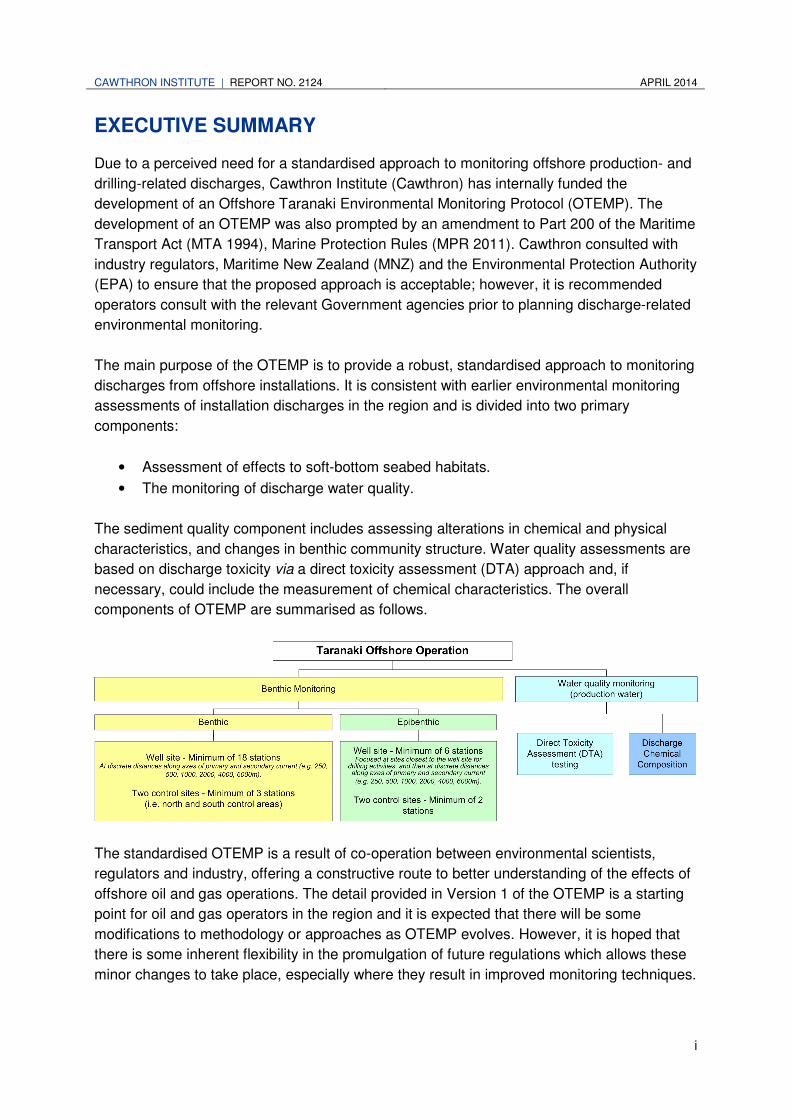
The main purpose of the OTEMP is to provide a robust, standardised approach to monitoring
discharges from offshore installations. It is consistent with earlier environmental monitoring
assessments of installation discharges in the region and is divided into two primary
components:
• Assessment of effects to soft-bottom seabed habitats.
• The monitoring of discharge water quality.
The sediment quality component includes assessing alterations in chemical and physical
characteristics, and changes in benthic community structure. Water quality assessments are
based on discharge toxicity via a direct toxicity assessment (DTA) approach and, if
necessary, could include the measurement of chemical characteristics. The overall
components of OTEMP are summarised as follows.
The standardised OTEMP is a result of co-operation between environmental scientists,
regulators and industry, offering a constructive route to better understanding of the effects of
offshore oil and gas operations. The detail provided in Version 1 of the OTEMP is a starting
point for oil and gas operators in the region and it is expected that there will be some
modifications to methodology or approaches as OTEMP evolves. However, it is hoped that
there is some inherent flexibility in the promulgation of future regulations which allows these
minor changes to take place, especially where they result in improved monitoring techniques.

CAWTHRON INSTITUTE | REPORT NO. 2124 APRIL 2014
iii
TABLE OF CONTENTS
EXECUTIVE SUMMARY ........................................................................................................ I
1. INTRODUCTION ........................................................................................................... 1
1.1. Background .................................................................................................................................................... 1
1.2. Aims ............................................................................................................................................................... 1
1.3. Structure ......................................................................................................................................................... 2
1.3.1. Sediment quality ........................................................................................................................................ 2
1.3.2. Water quality ............................................................................................................................................. 3
1.4. Limitations ...................................................................................................................................................... 3
1.4.1. Operational limitations ............................................................................................................................... 4
1.5. Discharge characteristics ............................................................................................................................... 7
1.5.1. General production-related discharges ..................................................................................................... 7
1.5.2. Exploration and development drilling discharges ...................................................................................... 9
1.5.3. Potentially toxic discharges ..................................................................................................................... 11
1.6. Volume and duration of discharge ................................................................................................................ 11
1.7. Fate of discharge: spatial extent and dilution ............................................................................................... 12
2. ENVIRONMENTAL MONITORING PLAN DESIGN.......................................................13
2.1. Site-specific Environmental Monitoring Plan synopsis .................................................................................. 13
3. MONITORING METHODS ............................................................................................15
3.1. Monitoring hypotheses ................................................................................................................................. 15
3.1.1. Effective monitoring to manage discharges ............................................................................................. 16
3.2. Benthic monitoring ........................................................................................................................................ 17
3.2.1. Station selection ...................................................................................................................................... 17
3.2.3. Sampling methodology ............................................................................................................................ 24
3.2.4. Epibenthic sampling ................................................................................................................................ 29
3.3. Water quality monitoring ............................................................................................................................... 31
3.3.1. Direct toxicity assessment — predictive monitoring ................................................................................ 31
3.3.2. Produced water constituent testing — observational monitoring ............................................................. 33
4. ANALYSES ...................................................................................................................34
4.1. Benthic samples ........................................................................................................................................... 34
4.1.1. Sediment analyses .................................................................................................................................. 34
4.1.2. Macrofaunal analyses ............................................................................................................................. 37
4.1.3. Epibenthic analysis.................................................................................................................................. 39
4.2. Water samples .............................................................................................................................................. 39
4.2.1. Direct toxicity assessment: ecotoxicity .................................................................................................... 39
5. TIMING AND FREQUENCY OF MONITORING ............................................................43
5.1. Benthic monitoring ........................................................................................................................................ 43
5.1.1. Production-related monitoring ................................................................................................................. 43
5.1.2. Exploration drilling monitoring ................................................................................................................. 43
5.1.3. Multi-well developmental drilling from existing production facilities ......................................................... 43
5.2. Water quality monitoring ............................................................................................................................... 44
6. ENVIRONMENTAL MONITORING PLAN DEVELOPMENT AND REPORTING ...........45
7. FURTHER CONSIDERATIONS ....................................................................................48
7.1. Developing clear monitoring processes ........................................................................................................ 48
APRIL 2014 REPORT NO. 2124 | CAWTHRON INSTITUTE
iv
7.2. Collective responsibilities ............................................................................................................................. 49
8. REFERENCES .............................................................................................................51
9. APPENDICES ...............................................................................................................54
LIST OF FIGURES
Figure 1. Generalised map of the offshore Taranaki setting, bathymetry, permitted production and exploration areas, and established well sites .............................................................. 6
Figure 2. Generalised example of the monitoring hypotheses H01 and adaptive management process. ............................................................................................................................. 17
Figure 3. Schematic diagram of generalised sampling station layout for drilling- and production-related monitoring plans. ................................................................................................... 20
Figure 4. Taranaki region showing previous and current control site locations. .............................. 22
Figure 5. Schematic diagram of suggested randomised control station allocation. ......................... 23
Figure 6. Double van Veen grab, approximate dimensions and functional features. ...................... 25
Figure 7. Schematic diagram of the double van Veen grab sampling process. ............................... 28
Figure 8. Schematic diagram of epibenthic component. .................................................................. 29
Figure 9. Images of a remotely operated video sled system. .......................................................... 30
Figure 10. Schematic diagram of production water discharge monitoring components and processes. ......................................................................................................................... 33
Figure 11. Schematic flow diagram of the Environmental Monitoring Plan reporting procedure, with communication pathways between relevant parties. ................................................. 47
LIST OF TABLES
Table 1. Summary of methods for the double and single grab techniques. ................................... 27
Table 2. Example of common analytical methods for sediments collected from sampling stations. ............................................................................................................................. 36
Table 3. Examples of potential biological statistical data analyses. ............................................... 38
LIST OF APPENDICES
Appendix 1. Schematic flow diagram of the proposed Offshore Taranaki Environmental Monitoring Protocol components and processes. ............................................................................... 54
Appendix 2. Environmental Monitoring Plan guideline documents. ...................................................... 55
Appendix 3. The MetOcean Solutions Ltd implementation of the Princeton Ocean Model for hindcasting the depth-averaged wind-driven and tidal currents. ...................................... 57
Appendix 4. A generic example of an Environmental Monitoring Plan as it might be used in conjunction with the Offshore Taranaki Environmental Monitoring Protocol, including the site-specific synopsis, deposition modelling, and area map showing location of the operation and the proposed sampling locations. .............................................................. 62
Appendix 5. Rationale for each sampling method. ............................................................................... 65

CAWTHRON INSTITUTE | REPORT NO. 2124 APRIL 2014
1
1. INTRODUCTION
1.1. Background
Until recently, there were no specific regulatory requirements that New Zealand
offshore oil and gas installations undertake environmental monitoring on the potential
impacts from operational discharges. This changed in 2010, with the Part 200
amendment to the Maritime Transport Act (MTA 1994) Marine Protection Rules (MPR
2011). The objective of Part 200 is to provide rules for offshore installations to help
prevent pollution of the marine environment by materials used or generated in
exploration, production and development. Part 200 deals specifically with discharges
of oil, other harmful substances and garbage, requiring operators to develop a
Discharge Management Plan (DMP), to promote the use of a ‘best practicable option’
to prevent or minimise adverse effects on the environment. As part of the DMP, an
Environmental Monitoring Plan (EMP) is required for all offshore installations, and it
must be approved by the Director of Maritime NZ. However, it is recognised that
further regulatory change may occur in the future, with the Environmental Protection
Authority (EPA) taking responsibility (from Maritime New Zealand; MNZ) for the
individual EMP component of the DMP.
This report provides recommendations for a standardised Offshore Taranaki
Environmental Monitoring Protocol (OTEMP), as illustrated in Appendix 1. To date,
the development of the OTEMP has been funded by the Cawthron Institute
(Cawthron) in response to a perceived need for a standardised approach to
monitoring discharges1 from offshore installations. Throughout the development of
OTEMP there has been significant input from industry operators (AWE Ltd, OMV Ltd
and STOS Ltd), MNZ and the EPA.
1.2. Aims
The overall aim of the OTEMP is to detect benthic ecological effects from offshore
operational discharges such as production water and drilling-related discharges (e.g.
from field developmental drilling and exploration drilling). In achieving this, specific
monitoring objectives are to:
• Provide a means of determining adverse ecological effects on benthic ecology
(including macrofaunal communities, and physical and / or chemical alterations)
that can be related or attributed to discharge activities.
• Assess the spatial extent and magnitude of project-related contamination / effects.
1 The term ‘discharge’ will be used from this point forward to relate to production and drilling discharges e.g.
exploration, development and production. Unless indicated otherwise, the terms ‘installations’ and ‘operations / operational’ will refer to exploration, development and production-related discharge activities.

APRIL 2014 REPORT NO. 2124 | CAWTHRON INSTITUTE
2
• Assess the toxicity of an effluent to ensure that its release into the aquatic
environment does not harm exposed biota.
• Accumulate site-specific benthic ecological data, recommended to be used for
testing predictions in an Environmental Impact Assessment (EIA)2.
• Ensure that regulatory guidelines and environmental standards are met.
• Assess the effectiveness of any implemented mitigation measures.
• Contribute to continuous improvement in the management of environmental
issues relating to offshore facilities.
• Assess the spatial extent and magnitude of drilling- and production-related
contamination.
• Provide an early warning of changes in the environment.
• Improve understanding of environmental cause-and-effect.
1.3. Structure
The proposed OTEMP is not a stand-alone monitoring document. It is intended to be
a guide (or reference document) for operators when designing EMPs for offshore
installations. Essentially, the EMP for each installation is proposed to be a brief site-
specific synopsis, using standardised OTEMP methodology (as described in Section
2.1 of this report).
The rationale for the OTEMP monitoring design, including specific analyses and
methodologies, has been explained in this document as thoroughly as possible.
Specific rationale has not been undertaken for every aspect of the protocol, so a
summary of the main documents and guides that were used to develop the OTEMP
are included in Appendix 2.
Internationally, programmes that monitor impacts of oil and gas operations, have
routinely investigated sediment and water quality. These two components form the
basis of the methods and monitoring designs recommended for the OTEMP, and are
outlined below.
1.3.1. Sediment quality
Contaminants in sediment and their effects on benthic organisms are routinely
monitored by industry and the scientific community (Ellis et al. 2012). Sediments are
the ultimate sink of persistent chemicals and particulate matter emitted from well
development and production activities. Internationally, contamination of sediments
and the effects on benthic organisms have been identified as key indicators of
2 Development of an Environmental Impact Assessment (EIA), which incorporates predictions/hypotheses (such
as scale of effects from discharges) is a recommendation made by OTEMP to strengthen the monitoring programme (explained in Section 10).

CAWTHRON INSTITUTE | REPORT NO. 2124 APRIL 2014
3
sediment quality. Methods to assess the quality of sediment and associated fauna
include:
• measurement of sediment grain size and chemistry
• assessment of benthic community structure
• sediment toxicity testing
These tests constitute what is commonly referred to as a ‘sediment quality triad’, an
integrative or weight of evidence approach (Chapman 1990). At this stage, OTEMP
only incorporates the first two components. However, if there is evidence3 of sediment
contamination, a sediment toxicity component can then be added to OTEMP and the
individual operator’s EMPs.
1.3.2. Water quality
Consistent with MNZ Part 200 recommendations, direct toxicity assessment (DTA)
(otherwise known as, whole effluent toxicity testing or WET) tests can be used to
monitor water quality at the immediate point of discharge. Where representative
samples are able to be taken, the discharge chemical characteristics (e.g. metals,
hydrocarbon concentrations and temperature) should also be measured (i.e. for
production water discharge and drilling fluids4).
As each oil and gas facility is different, OTEMP is intended to act only as a guide for
the design of offshore Taranaki oil and gas production-related discharge monitoring.
As such, it is not specifically designed for any one facility, and some of the limitations
associated with the OTEMP design are noted below.
1.4. Limitations
The current version of the OTEMP methodology is solely designed for monitoring soft
sediment substrate (i.e. silt and clay dominated size fractions). It is not necessarily
considered appropriate for other substrate types, i.e. is not intended for monitoring
reef environments, or substrates with coarser sized sediment fractions (e.g. pebbles
or boulders). The OTEMP is also not designed for near-shore sampling (e.g. within
the 12-mile limit) nor is it designed to be used in high value marine environments (as
specified in Beauford et al. 2009).
The OTEMP is specifically based around marine offshore exploration and production
permitted areas in the Taranaki Basin (or ‘offshore Taranaki’). There are a range of
3 If contaminant concentrations exceed the ANZECC (2000) sediment quality guidelines.
4 Cawthron is aiming to develop a database of drilling fluids, additives, and produced water ecotoxicity-levels on
NZ species. This should be used (along with standard Material Safety Data Sheets) to determine the potential ecological effects of discharge (in EIAs), and would aid assessment of potential ecological changes observed through environmental monitoring.

APRIL 2014 REPORT NO. 2124 | CAWTHRON INSTITUTE
4
facilities associated with the offshore Taranaki oil and gas production, development
and exploration (including appraisal well) operations. These include:
• FPSO — floating production, storage and offloading facilities
• well head platforms (manned and unmanned)
• drilling rigs
• jack-up rigs
• control areas.
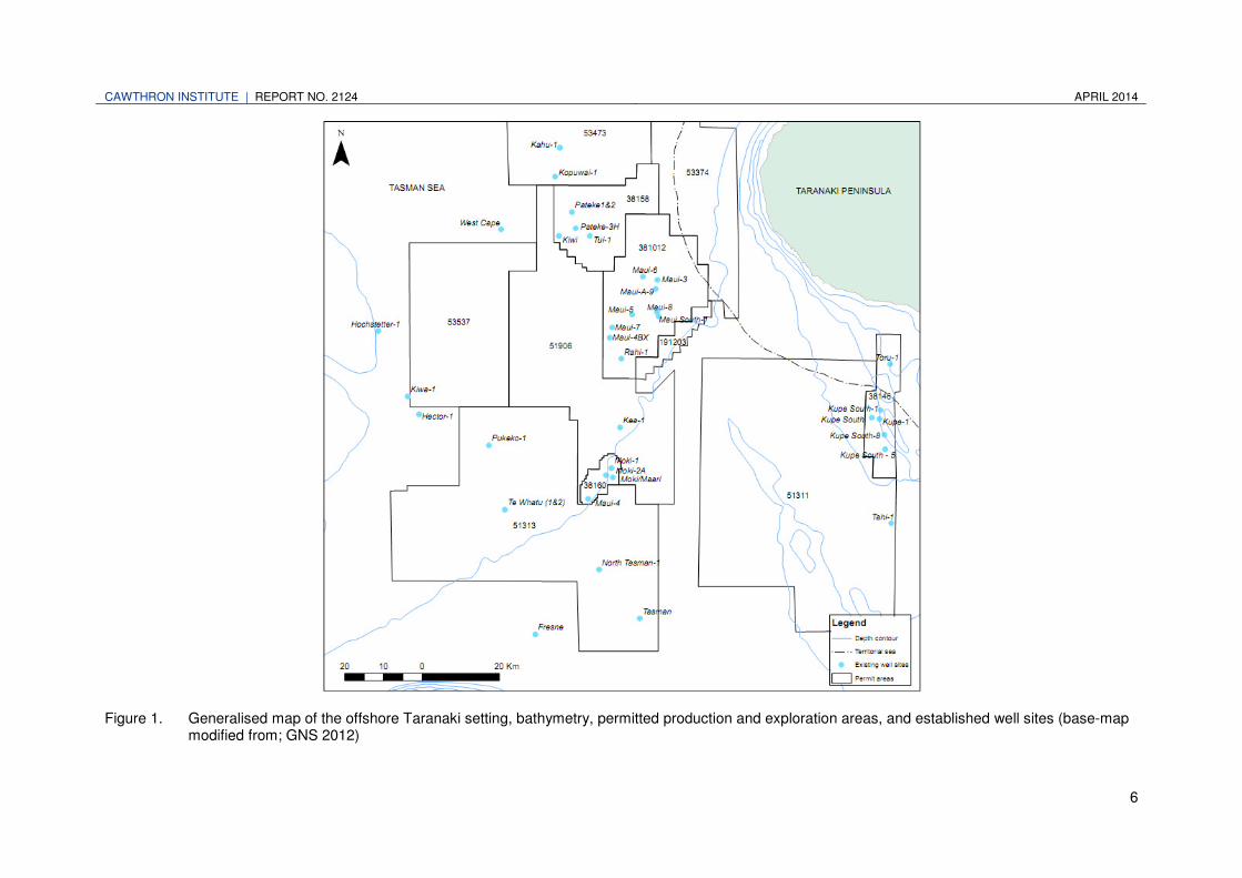
The OTEMP specific area (Figure 1) is delineated to the east by the territorial sea
outer limit (12 nautical miles or approximately 22 km off the coastal low-water mark).
The northern, southern and western extent is roughly bounded by the 80–150 m depth
contours. Any areas outside of the defined project setting are not within the scope of
this OTEMP.
Note: The OTEMP is considered a robust, starting point for offshore Taranaki drilling-
and production-related environmental monitoring plans. However, depending on
conditions and restrictions pertaining to each facility, there may be additional sampling
requirements (i.e. reallocated sampling stations due to confounding sub-surface
structures). It is highly recommended to seek professional scientific advice regarding
the applicability of OTEMP to any given facilities EMP, and to liaise with the regulating
authority to ensure the most appropriate monitoring techniques are employed.
1.4.1. Operational limitations
The inherent complexity in setting up and operating these facilities in the offshore
environment means that there are numerous operational constraints which preclude a
randomised approach to sampling around such facilities, making these areas
particularly difficult to sample. Factors include:
• anchor lines — snagging of sampling equipment
• FPSO lines — injection lines and off-loading lines could incur damage from
sampling equipment and vessels
• pipelines
• multiple well centres (sub-surface well heads)
• anthropogenic debris (nets, ropes, anchors etc.)
• ensuring there are appropriate representative control sites, outside zones of
influence of facilities and other man-made disturbances, but close enough to the
facility to be comparable
• oil, gear and personnel offloading / vessel movements
• the inherent danger associated with working around major hydrocarbon sources.
CAWTHRON INSTITUTE | REPORT NO. 2124 APRIL 2014
5
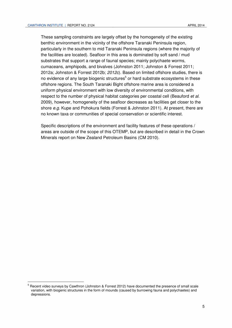
These sampling constraints are largely offset by the homogeneity of the existing
benthic environment in the vicinity of the offshore Taranaki Peninsula region,
particularly in the southern to mid Taranaki Peninsula regions (where the majority of
the facilities are located). Seafloor in this area is dominated by soft sand / mud
substrates that support a range of faunal species; mainly polychaete worms,
cumaceans, amphipods, and bivalves (Johnston 2011; Johnston & Forrest 2011;
2012a; Johnston & Forrest 2012b; 2012c). Based on limited offshore studies, there is
no evidence of any large biogenic structures5 or hard substrate ecosystems in these
offshore regions. The South Taranaki Bight offshore marine area is considered a
uniform physical environment with low diversity of environmental conditions, with
respect to the number of physical habitat categories per coastal cell (Beauford et al.
2009), however, homogeneity of the seafloor decreases as facilities get closer to the
shore e.g. Kupe and Pohokura fields (Forrest & Johnston 2011). At present, there are
no known taxa or communities of special conservation or scientific interest.
Specific descriptions of the environment and facility features of these operations /
areas are outside of the scope of this OTEMP, but are described in detail in the Crown
Minerals report on New Zealand Petroleum Basins (CM 2010).
5 Recent video surveys by Cawthron (Johnston & Forrest 2012) have documented the presence of small scale
variation, with biogenic structures in the form of mounds (caused by burrowing fauna and polychaetes) and depressions.
CAWTHRON INSTITUTE | REPORT NO. 2124 APRIL 2014
6
Figure 1. Generalised map of the offshore Taranaki setting, bathymetry, permitted production and exploration areas, and established well sites (base-map
modified from; GNS 2012)

CAWTHRON INSTITUTE | REPORT NO. 2124 APRIL 2014
7
1.5. Discharge characteristics
As OTEMP has been specifically designed to support discharge-related EMP design,
production water, and drilling related discharges (developmental and exploration
drilling) are characterised in the following sections.
1.5.1. General production-related discharges
Production operations can have multiple discharges to be considered, some of these
which may apply, are listed below:
• cements, slurries and sand —sand-blasting materials, and paint chips
• flushing and wash-down
• thermal discharge — heated water discharge (blow-down, cooling water, engine
cooling)
• hydro test and construction water
• sludge, ballast and tank bottoms.
• contaminated storm-water runoff
• accidental / chronic debris
• grey water and sewage / wastewater discharge
• production water — produced formation water (see below for specific constituents)
• discharges from supply vessels.
As produced water is generally the largest volume of aqueous discharge from
production operations, it is described in more detail in the following sections.
Produced water discharges (formation water)
Produced water includes formation water and injection6 water that is extracted along
with oil and gas during petroleum production. It is described in Neff et al. (2011) as, “a
complex mixture of dissolved and particulate organic and inorganic chemicals”. The
physical and chemical properties of produced water vary widely depending on origin
of the formation water being extracted i.e. the geologic age, depth, geochemistry,
chemical composition of the oil / gas phases in the reservoir, and additive chemicals
used for production. As produced waters are unique, Neff et al. (2011) recommend
that regionally specific studies are needed to address the environmental risks from
produced water discharge.
6 The extent of injection water extraction practices in offshore Taranaki is not known, but is thought to be low, or
not occurring at all. It is noted that the majority of offshore Taranaki systems are thought to extract oil by using energy provided by natural water driven mechanisms (e.g. aquifer expansion); pers. comm. Bruce Colgan; Shell Todd Oil Services (STOS).

APRIL 2014 REPORT NO. 2124 | CAWTHRON INSTITUTE
8
Over a lengthy geological time scale (millions of years), a variety of naturally occurring
compounds (inorganic salts, metals, radioisotopes, and a wide variety of organic
chemicals, primarily hydrocarbons) have been dissolved or dispersed naturally from
the geologic formations and along migration pathways. As a result of drilling and
production processes, these formation water compounds are discharged to sea.
Produced water also contains the same salts as seawater. The most abundant
inorganic ions in high-salinity produced water are, in order of relative abundance;
sodium, chloride, calcium, magnesium, potassium sulfate, bromide, bicarbonate, and
iodide. However, concentration ratios of many of these ions in produced water are
different to that of seawater, possibly contributing to the aquatic toxicity of produced
water. Most produced waters have salinities greater than that of seawater and are
therefore denser in comparison. The salinity7 of produced water can range from a few
parts per thousand (‰) to that of a saturated brine (approx. 300‰).
Production water can also have multiple additives (chemicals and constituents)
associated with it, which should be considered in analyses. Some of these are listed
below:
• Biocides: i.e. Sulphate-reducing bacteria (such as Desulfovibrio) can convert
sulphate ions to sulphide ions, which will corrode metal pipes and storage vessels.
Sulphate ions, in turn, are produced from elemental sulphur by the action of
sulphur oxidizing bacteria. One method of minimizing this effect is to reduce the
bacterial populations by adding biocides to the product stream. Biocides can be
volatile reactive substances; however, they are usually used at low
concentrations, of a few ppm at most in the effluent itself (Middleditch 1984).
• Coagulants: These include cationic (positive charge) and anionic (negative
charge) substances and quaternary ammonium compounds. Some coagulants
contain zinc chloride in concentrations of 5-30% (Middleditch 1984).
• Corrosion inhibitors: These are described in Middleditch (1984) as containing8
fatty amines, fatty acid amides, quaternary ammonium compounds, and fatty
amine salts. Almost all are cationic in nature. The amines are relatively toxic
toward fish, and the surface-active agents tend to coat the gills of fish. According
to Middleditch (1984) most of the residual corrosion inhibitor resides within the oil,
with less than 1 ppm remaining in the effluent.
• Cleaners and detergents: These are used for washing the platforms, usually
collect in separator tanks so that residual oil can be removed and can then be
included in produced water (Middleditch 1984). Concentrations of these
detergents would usually be low.
• Emulsion breakers: These may be non-ionic (no charge) or anionic (negative
charge) polymers and include suffocates and other esters as well as alkylene 7 Salinity of seawater = 32–36‰
8 May also contain some hydrocarbon components (pers. comm. Bruce Colgan; STOS)
CAWTHRON INSTITUTE | REPORT NO. 2124 APRIL 2014
9
oxides. Most are oil-soluble, but some are partially soluble in water. Low
concentrations of ethoxylates and low-molecular-weight acrylates might be
employed as dispersants.
• Paraffin control agents: The heavier paraffins can precipitate from the product
stream at ambient temperatures. Most control agents are fatty esters, which are
oil-soluble. Phenol adducts9 are also employed.
In addition to oil, produced water can contain both organic and inorganic contaminants
resulting from exposure to the oil reservoir and the various drilling and production
operations. Most investigations have emphasized the hydrocarbon and / or heavy
metal content of the effluents, but there is potential for other constituents as well
(Middleditch 1984).
If drilling is being proposed (as opposed to production), some of the primary
discharges that must be considered are described in the following sections.
1.5.2. Exploration and development drilling discharges
Exploration drilling often involves a single well head being drilled, whereas
developmental drilling frequently involves multiple wells around an existing producing
facility, with wells being drilled in succession. While more discharge can be expected
from developmental multi-well drilling, both processes can involve release of
discharges into the receiving environment; these discharges are described in the
following sections.
Drill cuttings
These consist of crushed rock generated by the drill as it penetrates the rock below
the seafloor. A significant portion of the drill cuttings can be retrieved from the
wellbore, and passed through solids control equipment to separate them from the
drilling fluid, where they are then discharged overboard (the drilling fluid is often re-
used down the well). A small proportion may be retained for geological information
purposes.
It is anticipated that this discharge will result in the short-term smothering of the
benthos, and changes to the sediment particle size, localised to the area of the
wellbore. Larger particles will settle near the bore, with finer particles dissipating with
the current.
Drilling fluids / muds
Drilling fluids are required to carry and release cuttings to the surface, cool and
lubricate the drill bit, prevent flow from the formation fluids to the borehole (which may
9 A new chemical species, each molecular entity of which is formed by direct combination of two separate
molecular entities in such a way that there is change in connectivity, but no loss, of atoms within the two separate molecular entities.
APRIL 2014 REPORT NO. 2124 | CAWTHRON INSTITUTE
10
result in a blowout) and prevent the collapse of the borehole. While the majority of this
fluid can be retrieved through the use of special shakers / screen configurations and
specialised cuttings drying equipment, some will remain adhered to the cuttings and
be discharged overboard.
Depending on the characteristics of the proposed well, the use of a Synthetic Based
Mud (SBM) or Water Based Muds (WBMs) will be required to keep drilling torque and
drag down. These muds are comprised of specific base chemicals (Neff et al. 2000),
as described below;
Synthetic-based mud
Synthetic-based mud (SBM) can contain synthetic hydrocarbons, ethers, esters, and
acetals. Total petroleum hydrocarbons (TPH), and esters are commonly used tracers
for determining SBM deposition / dispersal (Ellis et al. 2012). Examples of SBM
products know to be used in New Zealand are:
• Novaplus SBM; contains a C15-C18 internal olefin (IO) base, which can be traced
using extended TPH sediment analyses (TPHGC lab technique).
• Saraline SBM; contains a C8-C26 paraffin base, and can also be traced using
extended TPHGC.
Water-based mud
Water-based muds (WBMs) or water-based fluids (WBFs), used in many offshore
drilling operations, consist of water (fresh or salt), barite, clay, caustic soda, lignite,
lignosulfonates and / or water-soluble polymers. Note: barium sulphide (barite)
concentration in surface sediments is the most commonly used tracer material for
determining WBM deposition / dispersal, although is also used as a weighting material
in SBM occasionally (Ellis et al. 2012).
Additives
Additives are also incorporated into drilling muds and cementing for operational
requirements in order to solve some problems associated with particular drilling mud
properties. Examples of additives known to be used in New Zealand are listed in the
text box below.
The tracers used for determining additive deposition and dispersal will depend on the
specific types of additives used for drilling. A list of drilling mud additives must
therefore be supplied to the monitoring provider in order to ascertain whether the
present sediment chemistry analyses are sensitive to the product.
Tributyl phosphate controls foaming, ammonium bisulfite to remove oxygen, sodium
bicarbonate to remove excess calcium ions. Diesel fuel, mineral oil, or another
insoluble organic liquid may be added to a WBF at a concentration of a few percent to

CAWTHRON INSTITUTE | REPORT NO. 2124 APRIL 2014
11
improve the lubricity of the mud in difficult formations. The oil is dispersed in the water
phase and the cuttings remain water-wet.
Versawet is an organic surfactant (drilling fluid additive). If used, it is discharged to the
seabed with the drilling muds adhered to cuttings (however, the majority of the drilling
muds, and therefore any Versawet, will normally be retrieved). Total petroleum
hydrocarbons concentrations in the seabed sediment can be monitored to extrapolate
any discharges of this chemical.
Barite (consisting of BaSO4) is a weighting material and to date has been the most
frequently used. Ilmenite (FeTiO3), which has lower concentrations of trace metals
such as mercury, lead and cadmium, is increasingly being used as a replacement for
barite (Ellis et al. 2012).
1.5.3. Potentially toxic discharges
Of greatest interest from all of the potential production and drilling discharges
described, are the potentially toxic discharges. Testable chemicals that are potentially
toxic within the discharges are; metals / metalloids, drilling fluid residues (olefin,
paraffin etc.), TPHs and PAHs.
1.6. Volume and duration of discharge
Over the typical life of a producing oil field, the volume of produced water can exceed
10-fold, the volume of the oil produced (Ray & Ranier-Engelhardt 1992). The total
quantity of oil discharged by the offshore industry via cuttings, produced waters and
accidental spills can be high, representing inputs of carbon into the marine
environment (Patin 1999; Ellis et al. 2012).
Composition, volume and duration information from all discharges associated with oil
and gas production are not readily available (as they are not all measured e.g. sand-
blasting). However, as the ‘end-of-pipe’ production water is considered the highest
risk, and is able to be sampled, volumes and durations (flow) of end-of-pipe discharge
should also be recorded regularly by the operator (e.g. every 24 hrs, to determine
litres / day). The composition, volume and duration parameters of production water
discharges will vary among operators, however it is expected that this information will
be recorded and made available in order to provide an accurate prediction of
contaminant loading on the receiving environment, and to better assess / predict
ecological effects (particularly cumulative effects). Note: Discharge chemical
constituents (end-of-pipe sampling) can often be obtained from the operator, as an
existing part of their DMP agreement.
APRIL 2014 REPORT NO. 2124 | CAWTHRON INSTITUTE
12
1.7. Fate of discharge: spatial extent and dilution
Dispersion modelling studies on the fate of produced water report a rapid initial
dilution of most discharges by between 1:30–1:100 within the first few tens of metres
from the outfall. This is followed by a slower rate of dilution at greater distances (Neff
et al. 2011).
Site-specific numerical discharge models (e.g. Appendix 3) are recommended to be
used to better predict the fate (dilution and spatial extent) of chemical constituents in
produced water plumes. Using discharge modelling data, spatial scales of effects and
dilution concentrations of the site-specific discharge can be estimated (usually
reported in a preceding EIA document) and subsequently, site-specific monitoring
hypotheses can be developed (e.g. reasonable mixing zones, or expected zones of
influence, and primary direction discharge of flow).

CAWTHRON INSTITUTE | REPORT NO. 2124 APRIL 2014
13
2. ENVIRONMENTAL MONITORING PLAN DESIGN
As part of the overall Discharge Management Plan (DMP) process, individual
operators should provide a site-specific Environmental Monitoring Plan (EMP)
synopsis, to be submitted to the regulator for consideration. The EMP synopsis should
be site-specific, and should detail the design of the monitoring plan in the following
format. Provision of this synopsis is the responsibility of each individual operator and
should be used in addendum with only the most current OTEMP document.
2.1. Site-specific Environmental Monitoring Plan synopsis
An example of a site-specific synopsis can be found in Appendix 4, but includes the
following details:
• Operator name
• Facility description
• Monitoring hypotheses / aims / objectives (see Section 3.1)
• Field schedule
• Major axis of flow / minor axis of flow; refer to Appendix 4 for site-specific
current / rose diagram information for dominant current directions at facilities.
• A table of site-specific sampling stations locations (co-ordinates) and sampling
effort
• Proposed mixing zone / exclusion zone from facilities or activities
• Methodology10: e.g. benthic macrofauna, epibenthic biota, DTA testing, and
discharge chemical composition (DCC). Methods schematic to be attached and
refer to the Recommendations for an Offshore Taranaki Environmental Monitoring
Protocol: Production and drilling-related discharges
• Sampling stations: i.e. 18 (benthic) and three Southern Control (benthic); six
(Epibenthic) and two Southern Control (see attached maps)
• Sampling frequency: i.e. Annual (benthic, epibenthic, DTA) for three years then
review; quarterly (DCC) for one year, then review
• Reporting frequency: i.e. Annual (all parameters) within six months of field effort.
Subsequent reports should include analyses from previous sampling efforts and
be of a standard appropriate for external peer review. All raw data should be
included in the report(s)
• Specific sampling stations map
• Control site locations map
10
The proposed monitoring schematic diagram (Figure 1) and the Monitoring Protocol document e.g. “Taranaki Offshore Environmental Monitoring Protocol: Discharges,” are to be attached to the synopsis, and / or referred to in the synopsis methodology bullet point.

APRIL 2014 REPORT NO. 2124 | CAWTHRON INSTITUTE
14
• Appendices: Dispersion modelling; with dilution estimates (with rose diagram to
show hydrodynamic axes), and a table listing recent discharge volumes and
chemistry.
On completion of a monitoring survey, the operator should append the reports
(benthic ecological and DTA) issued by the science provider into the final discharge
management report (DMR), and submit these to the regulator. Specific detail on
monitoring frequency and reporting is available in Sections 5 and 6.
The sampling methods and processes behind the site-specific EMP synopsis are
described in more detail in the following sections.

CAWTHRON INSTITUTE | REPORT NO. 2124 APRIL 2014
15
3. MONITORING METHODS
Much of the site-specific synopsis is explanatory (e.g. operator name, facility
description, field schedule etc.) however, the other more complex components such
as; monitoring hypotheses, sampling station locations, sampling methods (method
validation and / or rationale are described in Appendix 5) and analyses have been
described in greater detail in the following sections. This forms the basis of the
OTEMP guidance document, and is expected to be used as a standardised
methodological reference for operator’s site-specific EMP synopses.
3.1. Monitoring hypotheses
Monitoring or null (H011) hypotheses are an analysis and reporting construct
established to assess effects predictions and can be applied to whole regions or
individual facilities. Effects predictions (scale and significance) are normally outlined
by the operator within an Environmental Impact Statement (using available data such
as hydrodynamic dispersal modelling, previous environmental effects monitoring data,
expert opinion or available literature).
In an Environmental Impact Assessment (EIA; usually completed prior to activities
occurring) the predicted environmental effects of a project can be evaluated, effects
rated12, and monitoring thresholds recommended. The effects and thresholds
specified in the EIA can then be used to construct the general monitoring hypotheses.
Rejecting the tested monitoring hypotheses could lead to adaptive management
measures.
General monitoring null hypotheses can be generated using effects ratings (as above)
and where possible, applicable guidelines (e.g. ANZECC 2000). Operators may also
elect to have a distance from discharge source (e.g. a ‘mixing zone’, as defined in
Rutherford et al. [1994]) where effects might be expected or considered reasonable to
occur. Examples13 of general monitoring hypotheses are as follows:
H0.1. There will be no effects to the physical sediment characteristics (grain size and
ash-free dry weight; AFDW), as a result of project discharges over time.
H0.2. Project discharges will not result in sediment chemistry concentrations to
exceed ISQG-Low guideline values (where applicable) or be significantly higher
than background/control concentrations.
H0.3. Project discharges will not cause biological effects.
11
A null hypothesis (H0) looks for the absence of an effect rather than the effect itself (sample observations result purely from chance).
12 The ‘effects ratings’ definitions are usually determined using risk assessment matrices and public consultation. Effect ratings could be defined specifically in the monitoring hypotheses as, outright mortality, sub-lethal harm, exclusion due to disturbance or percentage (%) change’.(e.g. < 20% change).
13 Example hypotheses should be adapted to suit individual project requirements, under consultation with a science provider and the regulatory body.

APRIL 2014 REPORT NO. 2124 | CAWTHRON INSTITUTE
16
H0.4. Incidental observations of project related debris will not be observed.
H0.5. Benthic sampling methodology will be sensitive enough to identify marine
environmental effects.
H0.6. Epibenthic observations will not detect biological effects.
H0.7. Effluent will not cause toxic effects (e.g. the median Lethal Concentration; LC50)
to laboratory biota with dilutions14 greater than 100:1 (1%), or dilutions below
environmental concern levels (ECL) outside of the mixing zone (e.g. 250 m).
3.1.1. Effective monitoring to manage discharges
By incorporating hypotheses (as above) in an EMP, monitoring can be given a defined
purpose; to determine whether project activities are resulting in the predicted
environmental effect, making it possible to adaptively manage specific components
(e.g. sedimentation) of the discharges, as illustrated in Figure 2.
If a monitoring hypothesis is rejected, further investigation should occur to better
answer questions on the nature and extent of the findings, e.g. sediment
characteristics and / or contaminant concentrations are not at background levels at
the far-field stations. Therefore, more far-field stations could be allocated in the
following survey to determine the true spatial extent of contamination. If the
hypotheses rejection then goes on to significantly affect the associated ecology, then
this would trigger adaptive management — and a change in the discharge activities /
process would have to be made (e.g. reduction in discharge / refining / alternative
disposal etc.).
Determination of ‘significant effects’ would be statistically-derived by default (i.e.
hypothesis testing: comparing the probability values with a chosen significance level).
However, significance could also be derived by comparing results with predetermined
levels (monitoring thresholds / effects ratings). If regional standardised monitoring
thresholds are aimed to be used, then it would be pertinent to investigate the
appropriate thresholds through a Taranaki-wide study. This could be achieved through
a desktop study, incorporating existing Taranaki data sets.
14
Initial H0/HA dilutions are to be refined using site-specific DTA test results, when they become available.

CAWTHRON INSTITUTE | REPORT NO. 2124 APRIL 2014
17
Figure 2. Generalised example of the monitoring hypotheses H01 and adaptive management process.
3.2. Benthic monitoring
3.2.1. Station selection
Monitoring stations
Scientific studies indicate that local conditions of current, depth, temperature, and
amount of material discharged all play a role in determining the severity and extent of
effects on seabed biological communities (Melton et al. 2000). Thus, it is reasonable
to assume that the axis, radiating from the discharge source, with the most dominant
directions of flow (i.e. down current from the discharge) will influence the deposition
patterns for discharges (Appendix 3). Based on this, the design of the benthic
component of the OTEMP is configured in relation to the dominant flow regime, in
order to isolate the effects of the primary dispersal pathways.
It is recommended that benthic and epibenthic stations are located along the cardinal
transect (major flow axis), as used in many similar surveys (Ellis & Schneider 1997;
Husky-Energy 2004; Petro-Canada 2007; Jogensen et al. 2011; Ellis et al. 2012).
Sample stations should be allocated in close proximity (e.g. within 250 m of the
discharge source) wherever safe and practicable in order to detect localised discharge
effects. Stations in close proximity are also likely to be useful for exploration-related
pre- and post-drilling surveys. There are fewer hazards associated with this way of
sampling because sampling would occur before drilling started, and then again once
drilling has stopped.
APRIL 2014 REPORT NO. 2124 | CAWTHRON INSTITUTE
18
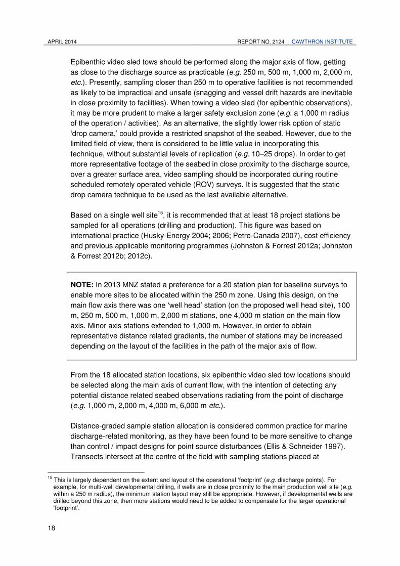
Epibenthic video sled tows should be performed along the major axis of flow, getting
as close to the discharge source as practicable (e.g. 250 m, 500 m, 1,000 m, 2,000 m,
etc.). Presently, sampling closer than 250 m to operative facilities is not recommended
as likely to be impractical and unsafe (snagging and vessel drift hazards are inevitable
in close proximity to facilities). When towing a video sled (for epibenthic observations),
it may be more prudent to make a larger safety exclusion zone (e.g. a 1,000 m radius
of the operation / activities). As an alternative, the slightly lower risk option of static
‘drop camera,’ could provide a restricted snapshot of the seabed. However, due to the
limited field of view, there is considered to be little value in incorporating this
technique, without substantial levels of replication (e.g. 10–25 drops). In order to get
more representative footage of the seabed in close proximity to the discharge source,
over a greater surface area, video sampling should be incorporated during routine
scheduled remotely operated vehicle (ROV) surveys. It is suggested that the static
drop camera technique to be used as the last available alternative.
Based on a single well site15, it is recommended that at least 18 project stations be
sampled for all operations (drilling and production). This figure was based on
international practice (Husky-Energy 2004; 2006; Petro-Canada 2007), cost efficiency
and previous applicable monitoring programmes (Johnston & Forrest 2012a; Johnston
& Forrest 2012b; 2012c).
NOTE: In 2013 MNZ stated a preference for a 20 station plan for baseline surveys to
enable more sites to be allocated within the 250 m zone. Using this design, on the
main flow axis there was one ‘well head’ station (on the proposed well head site), 100
m, 250 m, 500 m, 1,000 m, 2,000 m stations, one 4,000 m station on the main flow
axis. Minor axis stations extended to 1,000 m. However, in order to obtain
representative distance related gradients, the number of stations may be increased
depending on the layout of the facilities in the path of the major axis of flow.
From the 18 allocated station locations, six epibenthic video sled tow locations should
be selected along the main axis of current flow, with the intention of detecting any
potential distance related seabed observations radiating from the point of discharge
(e.g. 1,000 m, 2,000 m, 4,000 m, 6,000 m etc.).
Distance-graded sample station allocation is considered common practice for marine
discharge-related monitoring, as they have been found to be more sensitive to change
than control / impact designs for point source disturbances (Ellis & Schneider 1997).
Transects intersect at the centre of the field with sampling stations placed at
15
This is largely dependent on the extent and layout of the operational ‘footprint’ (e.g. discharge points). For example, for multi-well developmental drilling, if wells are in close proximity to the main production well site (e.g. within a 250 m radius), the minimum station layout may still be appropriate. However, if developmental wells are drilled beyond this zone, then more stations would need to be added to compensate for the larger operational ‘footprint’.
CAWTHRON INSTITUTE | REPORT NO. 2124 APRIL 2014
19
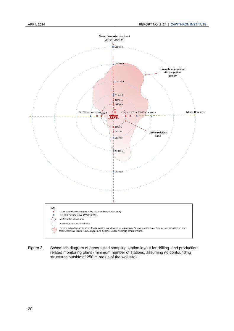
geometrically increasing distances from the centre. After characterising the projects
primary dispersal pathways16, station allocation is suggested as follows (as illustrated
in Figure 3):
• The major flow axes are recommended to be assigned 70–80% of station
allocation e.g. north-south axes at; 250, 500, 1,000, 2,000, 4,000, 6,000 m
• The minor flow axes are recommended to be assigned 20–30% of the overall
station allocation. This is to aid in discriminating observed benthic variation (i.e.
impacted vs. natural).
• Close proximity stations17 are advised to be included, as discharge related
benthic deposition effects are mostly likely to occur within 250–500 m of the
discharge source (Ellis et al. 2012) to the source. Approximately four 250 m
stations, and four 500 m stations (major and minor axes) should be allocated.
• Subsequent survey stations should be allocated with the consideration of
previous survey results. For example, if effects are found at the farthest station
during annual production survey, the following year additional stations should be
allocated at a greater distance to determine the spatial extent of the effect.
It is recommended that overall station allocation is made by an appropriately qualified
person (e.g. an experienced scientist).
16
From the predominant ocean currents, and discharge dispersal characteristics (Section 3.2.1; Appendix 3) 17
If closer stations are practicable for sampling then these should be included, however for the purposes of this example we are assuming a 250 m exclusion zone around the operation.
APRIL 2014 REPORT NO. 2124 | CAWTHRON INSTITUTE
20
Figure 3. Schematic diagram of generalised sampling station layout for drilling- and production-related monitoring plans (minimum number of stations, assuming no confounding structures outside of 250 m radius of the well site).

CAWTHRON INSTITUTE | REPORT NO. 2124 APRIL 2014
21
Control sites
It is recommended that regional control site(s) are utilised by more than one operator
and / or facility, rather than having a single control site for each facility. However, this
approach only works if operators jointly sample the two regional control sites during
each monitoring round (during the same season). Additionally, better use of resources
and greater continuity between operator’s results can be achieved by combining
control site sampling efforts.
It is known that discharge effects from production platforms can span distances
greater than 5 km, and up to 6 km in some cases (Bothner et al. 1985; Neff et al.
1989; Patin 1999). Generally control sites are placed at least 10–15 km away from the
centre of the point source (centre of the facility). Therefore, when selecting regional
control site locations a cumulative impacts approach that considers the locations of all
operators in the region has been used. These locations are subject to change18,
particularly if industry activity expands in the region.
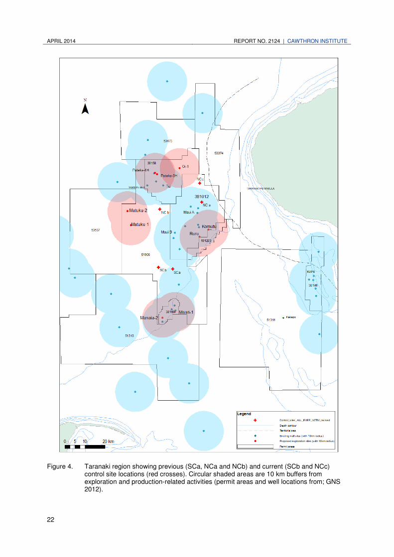
In 2010, a shared control site was successfully negotiated between operators,
however the chosen location was recently noted to be within the zone of influence of
neighbouring oil and gas operators (i.e. within 10 km; see Figure 4). The regional
control sites have since been moved to locations outside a 10 km radius of any
existing facility. Two regional control areas (North and South) have since been
selected and used in previous monitoring for operators in the region. It is envisaged
that the control site closest to each platform be used as the most applicable control.
For example, Figure 4 shows the Maari area is closest to the South Control site and
the Tui area to the North Control site. Data from both controls could then be used
cooperatively to improve the statistical analysis for every operator.
18
Control areas may become subject to contamination from other sources over time, therefore the suitability of control stations must be regularly evaluated.
APRIL 2014 REPORT NO. 2124 | CAWTHRON INSTITUTE
22
Figure 4. Taranaki region showing previous (SCa, NCa and NCb) and current (SCb and NCc) control site locations (red crosses). Circular shaded areas are 10 km buffers from exploration and production-related activities (permit areas and well locations from; GNS 2012).

CAWTHRON INSTITUTE | REPORT NO. 2124 APRIL 2014
23
Sampling within a control site
Prior to initiating the field component, control station locations should be determined.
In order to avoid oversampling the same control location, it is recommended that the
control area be of sufficient size (e.g. 25 hectares) to allow a random sampling
approach. One way of achieving this is overlaying the control site coordinates with a
grid (Figure 5). For a 25 hectare area, the one hectare grid squares become potential
sampling areas, with specific ‘station’ coordinates assigned to the centre of each
square.
It is suggested the three control sample stations are randomly selected by:
• Numbering each grid square from 1 to 25.
• Using a random number generator to select three numbers from between 1 to 25,
corresponding to each grid square.
• Replicate samples can be taken from anywhere within each of these grid squares.
• Record actual replicate sample locations within each grid square.
Figure 5. Schematic diagram of suggested randomised control station allocation.

APRIL 2014 REPORT NO. 2124 | CAWTHRON INSTITUTE
24
3.2.3. Sampling methodology
Benthic grab selection
In a recent literature review of environmental effects monitoring (EEM) programmes
around oil and gas platforms, the use of 0.1m² grabs for whole sediment samples was
identified as standard industry practice19 (Ellis et al. 2012). In order to increase the
statistical power and to meet best international standards, the OTEMP approach is to
collect sediment samples using a modified 0.1m2 van Veen grab (Figure 6). The
rationales for this method are outlined in the following points.
• Under the right deployment controls, the grab provides a large sample size
(0.1m²) of undisturbed sediment, therefore enabling a greater chance of detecting
ecological change.
• The van Veen is routinely used in deep water sites to assist uniform deployment
and is particularly effective in rough sea conditions. It has good release
mechanisms, weighted jaws and is steadied further in conjunction with a
stabilisation frame and provides a vertical descent to the bottom even when strong
underwater currents exist (IAEA 2003).
• Doors have screened openings to allow water to pass through on descent, and
also reduce washout on sample triggering (IAEA 2003).
• The larger opening at the bucket top provides less oscillatory shocks waves than
other grabs varieties (IAEA 2003). It is recognised that often with benthic grabs
there is a deployment wake if deployed too quickly — this pushes the lighter
surface sediments away, disturbing the sample. However, a controlled descent
can help minimise this potential bias, as it would be possible to slow the drop to an
optimal rate for adequate insertion into the sediments and the least amount of
surface disturbance. Additionally, if the drop is deployed at the same rate
(0.3 m sec-2), the amount of sediment disturbed should be consistent across all
the sampling, reducing any sampling bias.
• The van Veen grab is suitable for obtaining bulk samples ranging from soft and
fine-grained to sandy material for biological, hydrological and environmental
studies in deep water and strong currents (IAEA 2003).
• The use of a double van Veen grab (providing two concurrent grab samples;
Figure 6) can reduce sampling effort dramatically as complete and undisturbed
chemistry and macrofauna samples can be collected during the same grab event.
If varying methods (i.e. double van Veen vs. single van Veen) are to be used,
method validation20 should be undertaken (See Section 7.2).
20
This could be undertaken concurrently with scheduled offshore field surveys.

CAWTHRON INSTITUTE | REPORT NO. 2124 APRIL 2014
25
Figure 6. Double van Veen grab, approximate dimensions and functional features. Note: the volume calculations estimates are based on the volume of a
cylinder (one single grab bucket), and the van Veen grab is not a perfect cylindrical shape.

APRIL 2014 REPORT NO. 2124 | CAWTHRON INSTITUTE
26
Benthic grab sampling process
The process varies depending on whether a double van Veen or a single van Veen
grab is used. With the double van Veen (hereafter ‘double grab’), a total of three
deployments are required from each individual station (i.e. three grab buckets for
macrofaunal samples and three for sediment characteristics, as described in the
sections below and illustrated in Figure 7). Using the single van Veen grab (hereafter
‘single grab’), four deployments are necessary to obtain the required samples. The
following sections detail the sampling procedure using a double grab (also see
schematic in Figure 7). The variation in procedure when using a single grab is then
described (summarised in Table 1).
Note: If a double grab is not available, or malfunctions during the survey trip, then it is
acceptable to use a single van Veen grab. Method validation for these two techniques
found that macrofaunal results from both methods were able to be compared (Elvines
et al. 2013).
Macrofaunal sampling and incidental observations
One grab bucket per double grab deployment should be used to obtain macrofaunal
samples. The entire contents of the grab bucket should be sieved, through 0.5 mm
mesh to an approximately ‘fist sized’ amount of sediment (in order to protect soft
bodied fauna and for incidental analyses, see below). Remaining contents should be
placed in a labelled (large neck) 1 litre sample container with enough preservative
(e.g. ethanol / glyoxal) to cover the sample. The container should be turned over to
gently mix.
Sediments greater than 0.5 mm should be retained in the infaunal sample to be
analysed (in the laboratory), for any non-natural debris in the sediments. In particular,
paint-flecks, garnet grains, plastics, rust, oil conglomerations or any other observed
anthropogenic constituents to the sediments should be retained.
Sediment chemistry sampling
Double van Veen grab process
These samples should be taken from the second grab bucket, for each grab replicate,
in the following manner (summarised in Table 1):
1. To obtain the minimum allowable sample size21 for sediment grain-size (PGX) and
organic content (AFDW) analysis, a 63 mm diameter Perspex core should be used
to obtain a subsample of the top 5 cm of sediment. The sample should then be
placed in a labelled zip-lock bag.
2. Two standard 63 mm Perspex cores should be used to obtain two full sediment
cores from the grab. These should be photographed to record any evidence of
sediment type boundaries and stratigraphy. Following this, the top 5 cm of
21
Minimum acceptable sample weight at Hills Laboratories NZ Ltd =100g (2012).
CAWTHRON INSTITUTE | REPORT NO. 2124 APRIL 2014
27
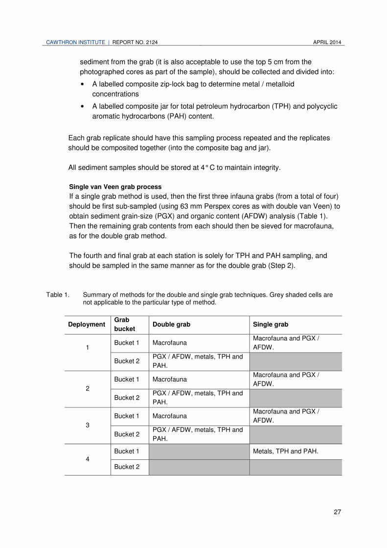
sediment from the grab (it is also acceptable to use the top 5 cm from the
photographed cores as part of the sample), should be collected and divided into:
• A labelled composite zip-lock bag to determine metal / metalloid
concentrations
• A labelled composite jar for total petroleum hydrocarbon (TPH) and polycyclic
aromatic hydrocarbons (PAH) content.
Each grab replicate should have this sampling process repeated and the replicates
should be composited together (into the composite bag and jar).
All sediment samples should be stored at 4° C to maintain integrity.
Single van Veen grab process
If a single grab method is used, then the first three infauna grabs (from a total of four)
should be first sub-sampled (using 63 mm Perspex cores as with double van Veen) to
obtain sediment grain-size (PGX) and organic content (AFDW) analysis (Table 1).
Then the remaining grab contents from each should then be sieved for macrofauna,
as for the double grab method.
The fourth and final grab at each station is solely for TPH and PAH sampling, and
should be sampled in the same manner as for the double grab (Step 2).
Table 1. Summary of methods for the double and single grab techniques. Grey shaded cells are not applicable to the particular type of method.
Deployment Grab
bucket Double grab Single grab
1
Bucket 1 Macrofauna Macrofauna and PGX /
AFDW.
Bucket 2 PGX / AFDW, metals, TPH and
PAH.
2
Bucket 1 Macrofauna Macrofauna and PGX /
AFDW.
Bucket 2 PGX / AFDW, metals, TPH and
PAH.
3
Bucket 1 Macrofauna Macrofauna and PGX /
AFDW.
Bucket 2 PGX / AFDW, metals, TPH and
PAH.
4 Bucket 1 Metals, TPH and PAH.
Bucket 2

APRIL 2014 REPORT NO. 2124 | CAWTHRON INSTITUTE
28
Figure 7. Schematic diagram of the double van Veen grab sampling process (excerpt from
Appendix 1). Analyses are detailed in Section 5.

CAWTHRON INSTITUTE | REPORT NO. 2124 APRIL 2014
29
3.2.4. Epibenthic sampling
Anthropogenic influences (drill cuttings etc.), epibenthic fauna and biogenic structures
should be determined by a total of eight epibenthic video sled tows of 250 m in length
(as mentioned in Section 3.2). Six of these should be along each of the major axes
radiating from the well site (as close to the well site as practicable) with particular
focus on the sites closest to the facilities i.e. the 250 m and 500 m stations on the
dominant flow axes. Two video sled tows should be performed at each control site.
The video sampling process is summarised in Figure 8.
Video sled
Semi-quantitative epibenthic data can be obtained from video footage of the seafloor.
A remotely operated video sled (ROVS) system can be effective, and involves simply
attaching a video system to a weighted sled frame (see Figure 9). It is suggested that
video footage at each site is at least two minutes duration.
Figure 8. Schematic diagram of epibenthic component (excerpt from Appendix 1).

APRIL 2014 REPORT NO. 2124 | CAWTHRON INSTITUTE
30
Figure 9. Images of a remotely operated video sled (ROVS) system. Top left: ROVS set up. Top right: ROVS console. Middle: Umbilical spool. Bottom: Schematic diagram of ROVS (design and functional features).

CAWTHRON INSTITUTE | REPORT NO. 2124 APRIL 2014
31
3.3. Water quality monitoring
At this stage of the OTEMP, only produced water is recommended for direct toxicity
assessment (DTA testing). Due to inherent difficulty in obtaining representative
samples, testing recommendations in OTEMP do not currently include any other
discharge types (e.g. drill cuttings, platform runoff etc.).
A greater degree of confidence in determining the toxicity of production water can be
obtained using both predictive and observational monitoring techniques
(Middleditch 1984). Observational monitoring techniques are those that are
undertaken in situ, whereas predictive techniques include extrapolating lab or
modelling results to determine potential effects in the field. Both components of water
discharge monitoring are summarised in Figure 10.
3.3.1. Direct toxicity assessment — predictive monitoring
To achieve the predictive monitoring component, OTEMP recommends DTA testing (a
series of bioassay experiments) of the appropriate discharge effluents is performed.
Conducting the OTEMP DTA requires a sample of production water, receiving
seawater, and laboratory-derived artificial sea-water (for serial dilutions). Descriptions
of each are included below, as well as a schematic overview in Figure 10.
Production water sample
A 5 L sample of production water should be collected from the point of discharge. This
sample is made into serial dilutions for bioassays, standardised by the USEPA (2002).
Receiving water sample
This sample (5 L) can be used to determine whether the receiving water itself has any
background toxicity (e.g. toxicity from other sources). A DTA can be performed
directly on an undiluted receiving water receiving water sample, collected from outside
the facilities influence (>10 km).
Receiving water should also be used to assess the spatial extent of toxicity from
production discharges, particularly if no dilution studies have been undertaken at the
facility22. It is recommended that an initial receiving water sample (5 L) is obtained
from the major axes of flow, at a distance of 250 m (Figure 3). If toxicity is detected in
this sample, further sampling should be undertaken (i.e. additional samples can be
taken at graded distances from the discharge source, and then used in a DTA), to
define these toxicity boundaries and to determine if toxicity is attributable to the
production-related discharges.
Note: there may be practical difficulties in obtaining receiving water samples (e.g.
timing, transport and identification of non-impacted areas). Therefore, it is important
22
In the absence of dilution studies around the discharge point, the trigger level determined by the DTA cannot predict spatial extent of toxicity.
APRIL 2014 REPORT NO. 2124 | CAWTHRON INSTITUTE
32
that collection location, difficulties encountered, date and the person responsible for
sampling be recorded and supplied with all collected samples.
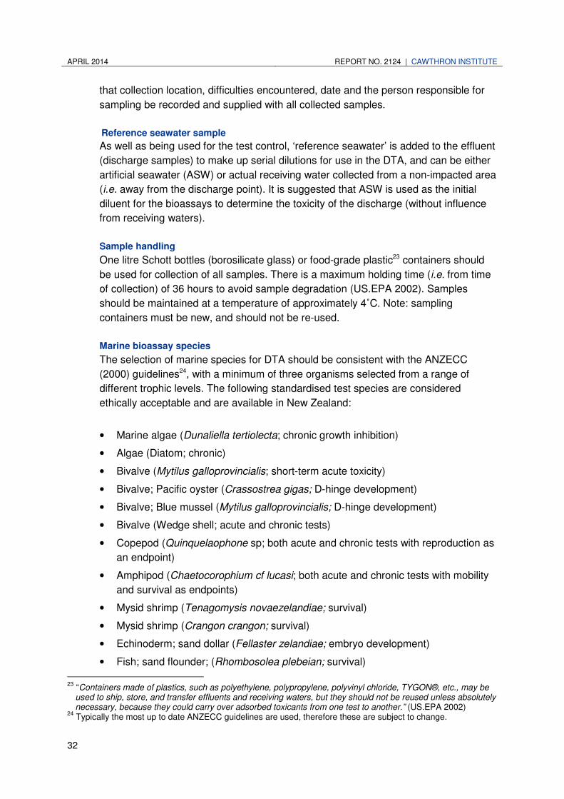
Reference seawater sample
As well as being used for the test control, ‘reference seawater’ is added to the effluent
(discharge samples) to make up serial dilutions for use in the DTA, and can be either
artificial seawater (ASW) or actual receiving water collected from a non-impacted area
(i.e. away from the discharge point). It is suggested that ASW is used as the initial
diluent for the bioassays to determine the toxicity of the discharge (without influence
from receiving waters).
Sample handling
One litre Schott bottles (borosilicate glass) or food-grade plastic23 containers should
be used for collection of all samples. There is a maximum holding time (i.e. from time
of collection) of 36 hours to avoid sample degradation (US.EPA 2002). Samples
should be maintained at a temperature of approximately 4˚C. Note: sampling
containers must be new, and should not be re-used.
Marine bioassay species
The selection of marine species for DTA should be consistent with the ANZECC
(2000) guidelines24, with a minimum of three organisms selected from a range of
different trophic levels. The following standardised test species are considered
ethically acceptable and are available in New Zealand:
• Marine algae (Dunaliella tertiolecta; chronic growth inhibition)
• Algae (Diatom; chronic)
• Bivalve (Mytilus galloprovincialis; short-term acute toxicity)
• Bivalve; Pacific oyster (Crassostrea gigas; D-hinge development)
• Bivalve; Blue mussel (Mytilus galloprovincialis; D-hinge development)
• Bivalve (Wedge shell; acute and chronic tests)
• Copepod (Quinquelaophone sp; both acute and chronic tests with reproduction as
an endpoint)
• Amphipod (Chaetocorophium cf lucasi; both acute and chronic tests with mobility
and survival as endpoints)
• Mysid shrimp (Tenagomysis novaezelandiae; survival)
• Mysid shrimp (Crangon crangon; survival)
• Echinoderm; sand dollar (Fellaster zelandiae; embryo development)
• Fish; sand flounder; (Rhombosolea plebeian; survival)
23
“Containers made of plastics, such as polyethylene, polypropylene, polyvinyl chloride, TYGON®, etc., may be used to ship, store, and transfer effluents and receiving waters, but they should not be reused unless absolutely necessary, because they could carry over adsorbed toxicants from one test to another.” (US.EPA 2002)
24 Typically the most up to date ANZECC guidelines are used, therefore these are subject to change.

CAWTHRON INSTITUTE | REPORT NO. 2124 APRIL 2014
33
• Bacteria (Microtox; survival).
3.3.2. Produced water constituent testing — observational monitoring
Testing of 24-hour composite produced water samples to determine chemical
constituents is undertaken by the operator as part of their overall DMP (Figure 10).
Direct testing of the constituents however can be undertaken as a second tier of
discharge effluent monitoring as part of the OTEMP if the DTA trigger points are
reached e.g. rejection of null hypotheses (Section 3.1). For example, to determine
which chemical / s is responsible for the observed toxicity, concentrations of metals,
or known additive constituents (etc.) can be measured.
Figure 10. Schematic diagram of production water discharge monitoring components and
processes (excerpt from Appendix 1).

APRIL 2014 REPORT NO. 2124 | CAWTHRON INSTITUTE
34
4. ANALYSES
4.1. Benthic samples
4.1.1. Sediment analyses
Chemical contaminants are primarily retained within fine sediments, metals especially,
can adsorb to particulates and may accumulate over long time periods. The full suite
of proposed analyses and their respective analytical methodology are presented in
Table 2.
Particle grain size
The analysis of sediment texture (particle grain size distribution) provides an important
measure of the physical characteristics that is used to investigate and interpret
differences between sites for other environmental parameters. Additionally, texture
plays an important role in constraining the ecological communities that are associated
with a given benthic area. For example, the types of biota found in muddy sediments
are generally very different to those in sandy environments. Therefore, sediment
texture is a useful and inexpensive measure of the physical characteristics of a
benthic environment, which can be used in combination with other techniques to
facilitate interpretations of changes (over time) and differences between sites.
Organic content
Sediment organic content or ash-free dry weight (AFDW) should be used as a
measure of the relative state of organic enrichment in benthic habitats. Increases in
organic matter production and retention can cause excessive nutrient
loading / eutrophication in a benthic soft bottom environment with consequent
potential for the development of anoxic conditions. In addition high organic content
can be related to high contaminant concentrations. For instance, muddy sediments
may be associated with increased organic content, which in turn, can facilitate the
binding of trace / heavy metal contaminants to the sediments.
Metals / metalloids
Trace metals / metalloids are associated with oil production and drilling processes, for
example barium, cadmium, chromium, copper, lead, mercury, nickel, silver and zinc
are commonly studied in relation to production water and drilling activities (Ray &
Ranier-Engelhardt 1992). The Taranaki offshore environment has natural
accumulations of soft sediments, and in these environments there is potential for fine
sediments to adsorb and retain higher concentrations of metals that may be
associated with oil production and drilling operations (Ray & Ranier-Engelhardt 1992).
However, it is noted that heavy metals in such tightly adsorbed forms have much
lower bioavailability to marine animals than they would if they were in solution (i.e. in
the water column). The suite of metals analysed should consist of a combination of
ubiquitous contaminants (e.g. cadmium, lead and zinc) along with several constituents
that are specifically related to drilling and production activities, such as the use of
CAWTHRON INSTITUTE | REPORT NO. 2124 APRIL 2014
35
water-based drilling muds (e.g. barium, chromium) and synthetic drilling muds (e.g.
total petroleum hydrocarbons).
Bentonite clays and compounds such as barite (barium sulphate) are often
incorporated into drilling muds and are also associated with production discharges
(Ray & Ranier-Engelhardt 1992; Neff et al. 2011). Barite has the potential to smother
immobile benthic species, however, it is not normally considered toxic and is not
commonly analysed as an environmental contaminant in marine sediments (unless
associated with drilling or production). Sneddon (2011) stated that sulphates occurring
in seawater ensure that barium is unlikely to occur in dissolved form and its bio-
availability is generally limited by barite precipitation. Barite is considered a tracer
element associated with production water, and for drilling muds. It was therefore
included in the programme to determine baseline / background levels of the metal with
which to compare future dispersal trends and to help determine the source of any
historical disturbance patterns that may emerge in future monitoring.
Sediment contaminant concentrations (from trace metal analyses) are suggested to
be compared against national sediment quality criteria (ANZECC 2000). The aim of
the guidelines is to predict ‘acceptable’ levels of contaminants in aquatic sediments,
above which adverse ecological effects may occur. The criteria are defined as Interim
Sediment Quality Guideline-Low (ISQG-Low) and -High (ISQG-High) levels,
representing two distinct thresholds above which biological effects may occur. The
guidelines are based on statistical models of toxicity data used to provide a level of
probability for detecting adverse effects at particular contaminant levels.
Total petroleum hydrocarbons
Total petroleum hydrocarbons (TPH) include a broad range of several hundred
chemical compounds associated with crude oil. These have the potential to
contaminate the surrounding marine benthic sediments and waters associated with
production fluids (Ray & Ranier-Engelhardt 1992). Generally, the amount of TPH
found in a sediment sample is useful as an indicator of petroleum contamination at
that site from production water, or from the discharge of synthetic drilling fluids (e.g.
elevated levels of olefin and paraffin in the sediments). By dividing TPH into groups
(fractions) of different chain length that behave similarly in the soil or water,
assumptions can be made about the potential effects of the TPH fractions found. For
example, heavier fractions can accumulate in the sediment on the sea floor, which
may affect bottom-feeding fish and benthic organisms, and lighter fractions may float
to the surface, with little effect on the benthic biota.
Polycyclic aromatic hydrocarbons
Polycyclic aromatic hydrocarbon (PAH) content is also characteristic of production
fluids and drilling muds. The PAHs, such as anthracene and pyrene, will not transform
into a gaseous phase, and will stay in the marine environment, undergoing complex
reactions (e.g. oxidations and biodegradation) until they form more soluble
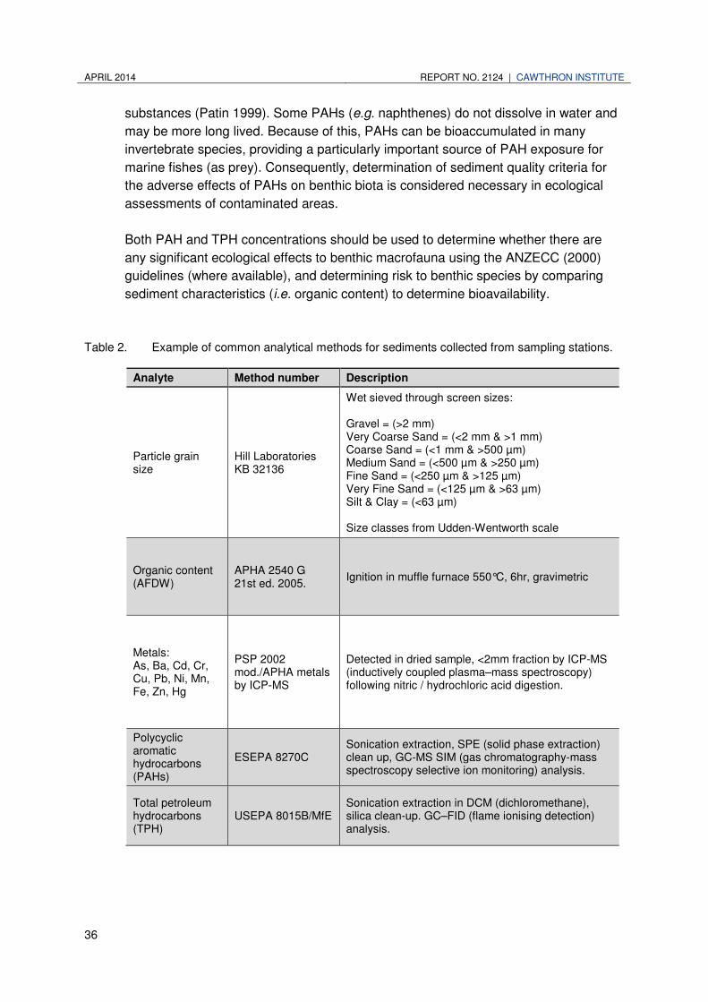
APRIL 2014 REPORT NO. 2124 | CAWTHRON INSTITUTE
36
substances (Patin 1999). Some PAHs (e.g. naphthenes) do not dissolve in water and
may be more long lived. Because of this, PAHs can be bioaccumulated in many
invertebrate species, providing a particularly important source of PAH exposure for
marine fishes (as prey). Consequently, determination of sediment quality criteria for
the adverse effects of PAHs on benthic biota is considered necessary in ecological
assessments of contaminated areas.
Both PAH and TPH concentrations should be used to determine whether there are
any significant ecological effects to benthic macrofauna using the ANZECC (2000)
guidelines (where available), and determining risk to benthic species by comparing
sediment characteristics (i.e. organic content) to determine bioavailability.
Table 2. Example of common analytical methods for sediments collected from sampling stations.
Analyte Method number Description
Particle grain size
Hill Laboratories KB 32136
Wet sieved through screen sizes: Gravel = (>2 mm) Very Coarse Sand = (<2 mm & >1 mm) Coarse Sand = (<1 mm & >500 µm) Medium Sand = (<500 µm & >250 µm) Fine Sand = (<250 µm & >125 µm) Very Fine Sand = (<125 µm & >63 µm) Silt & Clay = (<63 µm) Size classes from Udden-Wentworth scale
Organic content (AFDW)
APHA 2540 G 21st ed. 2005.
Ignition in muffle furnace 550°C, 6hr, gravimetric
Metals: As, Ba, Cd, Cr, Cu, Pb, Ni, Mn, Fe, Zn, Hg
PSP 2002 mod./APHA metals by ICP-MS
Detected in dried sample, <2mm fraction by ICP-MS (inductively coupled plasma–mass spectroscopy) following nitric / hydrochloric acid digestion.
Polycyclic aromatic hydrocarbons (PAHs)
ESEPA 8270C Sonication extraction, SPE (solid phase extraction) clean up, GC-MS SIM (gas chromatography-mass spectroscopy selective ion monitoring) analysis.
Total petroleum hydrocarbons (TPH)
USEPA 8015B/MfE Sonication extraction in DCM (dichloromethane), silica clean-up. GC–FID (flame ionising detection) analysis.

CAWTHRON INSTITUTE | REPORT NO. 2124 APRIL 2014
37
4.1.2. Macrofaunal analyses
Benthic invertebrates are to be used as environmental indicators of biological integrity.
As many benthic invertebrates are sessile, they can integrate effects of pollutants over
time, and are therefore sensitive to any changes in sediment and water quality (Gray
et al. 1990). Additionally, some benthic species can be very tolerant in certain
conditions (e.g. organic enrichment and hydrocarbon contamination) and in such
situations they can thrive, dominating the macrofaunal community composition. This
means they are frequently used as monitoring indicators because of the following:
• they are found in most aquatic habitats
• are relatively simple to collect
• can indicate water quality conditions or ecosystem health (Patin 1999)
• are consumed by a wide range of wildlife species (i.e. fish, amphibians, reptiles,
birds, and mammals)
• can be used to identify significant ecological change.
In the laboratory, macrofauna25 within the preserved samples should be identified to
the lowest practicable taxonomic level and counted with the aid of a binocular
microscope.
Macrofaunal data analyses
To detect whether there are any significant differences detected in macrofaunal
assemblages related to sampling axes, sampling distance, control sites or years,
macrofaunal data should be analysed using statistical software such as the PRIMER
v6 software (v. 6.1.6©PRIMER-E 2000; Clarke & Warwick 1994; Clarke & Gorley
2001). PRIMER is a multivariate statistical package for ecologists supporting a wide
range of complex functions. PRIMER is now considered a ‘standard’ for marine
community and biodiversity research, and is also widely used commercially for
assessing environmental impacts of discharges, mining, oilfields, trawling and
aquaculture. For industry continuity PRIMER (V6.1.6) is considered an appropriate
statistical package. Useful PRIMER functions for detecting community differences are
DIVERSE (principal community indices; Table 3), multi-dimensional scaling (MDS)
and cluster diagrams, ANOSIM (Analysis of Similarity), SIMPER (Similarity
Percentages), BEST (trend correlation), and PERMAnova (Permutational multivariate
analysis of variance).
25
Macrofauna are the ecological assemblage of small animals, larger than 0.5 mm.

APRIL 2014 REPORT NO. 2124 | CAWTHRON INSTITUTE
38
Table 3. Examples of potential biological statistical data analyses.
Index Equation Description
Richness (N) Count (taxa) Total number of taxa in a sample
Abundance (S) Sum (n) Total number of individual organisms in a sample
Evenness (J’) J’ = H’/Loge(S)
Pielou’s evenness. A measure of equitability, or how evenly the individuals are distributed among the different species. Values can theoretically range from 0.00 to 1.00, where a high value indicates an even distribution and a low value indicates an uneven distribution or dominance by a few taxa.
Diversity (H’ loge) H’ = -SUM(Pi*loge(Pi))
Shannon-Wiener diversity index (log-e base). A diversity index that describes, in a single number, the different types and amounts of animals present in a collection. Varies with both the number of species and the relative distribution of individual organisms among the species. The index ranges from 0 for communities containing a single species to high values for communities containing many species with each represented by a small number of individuals.
Incidental observations of debris
Debris remaining in the macrofaunal samples (i.e. >0.5 mm diameter) should also be
examined and recorded concurrently with the macrofaunal analysis. Debris that might
be expected from platform and FPSO-type facilities include (but are not limited to)
paint-flecks, garnet grains, plastics, rust and small oil conglomerations.
This is not intended to be a quantitative assessment; rather it does provide another
simple technique of ascertaining relative levels of platform-related debris (compared
to background levels) accumulating in the sediments. If significant amounts of industry
related debris are detected, a quantitative assessment method should be employed.
The relative abundance of any observed debris within macrofaunal samples should be
listed in a table, and any notable distance or directional related relative abundance
gradients described. We recommend specifying the debris relative abundance
classifications. As an example, relative abundance of paint-flecks (a single piece = 1
occurrence) could be classified as:
• Trace: 1–2 occurrences
• Low: 2–5 occurrences
• Common: 6–10 occurrences
• Abundant: greater than 10 occurrences

CAWTHRON INSTITUTE | REPORT NO. 2124 APRIL 2014
39
After analyses, incidental debris should be retained for at least three months in case
further analyses are required.
4.1.3. Epibenthic analysis
Video sled footage
Epibenthic species and demersal26 fish observed in the video footage should be
identified to lowest practicable taxonomic level or the most likely recognisable taxa
(and grouped per station). Additionally, visible biogenic or anthropogenic related
seafloor structures are should also be recorded (e.g. burrow holes, mounds etc.).
Observations can then be compared between stations (and control sites) and
significant differences interpreted with respect to factors such as substrate
characteristics (e.g. grain size, AFDW etc.).
4.2. Water samples
4.2.1. Direct toxicity assessment: ecotoxicity
Direct toxicity assessment bioassays fall into two general categories:
1. Static tests, which expose organisms to a given dilution of standing water for the
duration of the test.
2. Flow-through tests, which expose organisms to a continuous flow of ‘fresh’ effluent
at a given dilution.
Due to the characteristics of the discharge site (oceanic setting, significant water
depths), it is recommended that DTA uses static tests, as this method suitably mimics
exposure in the plume-affected water column. Flow-through tests should only be
considered if there is a particular concern of chronic exposure to diluted effluent e.g. if
it is shown that benthic or other sessile communities may be exposed to ecologically
significant concentrations (i.e. if the null / monitoring hypotheses is rejected).
Toxicity testing of representative samples of the discharge water from the facilities
should be carried out for each of the selected test species, using serial dilutions. DTA
test results should be interpreted using specific biological endpoints, as discussed in
the following section.
Biological end points
A DTA must incorporate biological endpoints that will most likely be predictive of
effects, not only to individual organisms, but also to whole populations and
ecosystems. To achieve this aim, the use of biological endpoints validated for
26
Demersal fish live and feed on or near the seafloor (e.g. flatfish)
APRIL 2014 REPORT NO. 2124 | CAWTHRON INSTITUTE
40
predicting these wider effects is recommended. Endpoints are classified into their
respective toxicity types; ‘acute’ and ‘chronic’.
• Acute toxicity is usually assed using lethality as the endpoint. It is usually
determined in controlled laboratory animal exposure studies of short duration (2–4
days). Lethality as an endpoint has limited ability to predict long-term sub-lethal
effects often associated with exposures to low levels of effluent.
• Chronic (or sub-lethal), endpoints can include changes in reproduction, growth,
metabolism, behaviour or other biological variables. These measures are more
sensitive and allow greater confidence when extrapolating effects to the
population level (ANZECC 2000).
To provide a comprehensive and robust predictive assessment of potential adverse
effects of the effluent to the surrounding environment, the DTA should incorporate a
variety of biological acute and chronic endpoints. Note: Any measure of effect in a
bioassay must specify the test type, the duration of the exposure, and the level of
effect measured. Test results are meaningless if such detail is unavailable.
Minimising variation in toxicity testing
The DTA must have robust quality assurance / quality control (QA / QC) measures to
ensure the tests are valid and reproducible. In other words, the results of a test should
be consistent when the test is repeated within and outside of any given laboratory. As
outlined in ANZECC (2000), the factors of major concern are analyst experience and
test organism health / condition. For robust results, an appropriate QA programme to
incorporate QC parameters is recommended. Guidance on QA / QC for DTA can be
found in ANZECC (2000).
Direct toxicity assessment output parameters
Results of a DTA typically output the ‘Effective Concentration’, ‘No Observable Effect
Concentration’, and ‘Lowest Observable Effect Concentration’ parameters to refer to
the toxicity of the effluent dilution to the tested organism. Each of these terms is
described in detail in the following paragraphs. For further detail on other methods of
statistical analyses refer to ANZECC 2000, Volume 2: Section 8.3.6.
Effective Concentration (EC) is the concentration of substance or material that is
estimated to be lethal to a proportion (x%) of the test organisms after a defined period
of exposure (t). This is an acute toxicity indicator. This kind of endpoint allows for the
classification and the comparison of the toxic potency or intensity of different
chemicals. More terms can be derived to describe specific effects (e.g. lethality,
inhibition), for example:
• Lethal Concentration (LCx-t) is the concentration of substance or material
that is estimated to be lethal to a proportion (x%) of the test organisms after a
CAWTHRON INSTITUTE | REPORT NO. 2124 APRIL 2014
41
defined period of exposure (t). This is an acute toxicity indicator. A dilution
presented with LC50-96hr would describe the concentration at which 50% of the
organisms have died after a period of 96 hours.
• Inhibitory Concentration (ICx-t) is the concentration of substance or material
that is estimated to have an inhibitory effect (e.g. growth, mobility) on a
proportion (x%) of the test organisms after a defined period of exposure (t).
This is a chronic toxicity indicator.
Lowest Observed Effect Concentration (LOEC) is statistically derived, and
represents the lowest concentration of a test substance or material which is observed
to have a statistically significant adverse effect on the test organisms for a defined
time of exposure and under the test conditions, relative to control.
No Observed Effect Concentration (NOEC) is also statistically derived, and
represents the highest concentration of a test substance or material which is observed
not to have a statistically significant adverse effect on the test organisms for a defined
time of exposure and under the test conditions, relative to control.
Application to the receiving environment
To give an overall indication of effluent toxicity to the biota in the receiving
environment, various statistically derived measures can be used. For example the
‘Threshold Effect Concentration’ or ‘Environmental Concern Level’, which both
incorporate results from each bioassay in the DTA.
Threshold Effect Concentration (TEC) is the geometric mean of the lowest NOEC
and LOEC in the DTA. TEC can be used to estimate ‘safe’ concentrations of a
discharge, taking into account receiving environment dilution. For example, a TEC
value of 1% would require 100:1 dilution to exhibit no toxic effect while a TEC of 50%
would require only 2:1 dilution.
Environmental Concern Level (ECL) is defined as that concentration of a chemical
which may cause adverse environmental effects (OECD 1995). Environmental
Concern Level (ECL) is derived from the lowest NOEC (for chronic measures) or EC
in the DTA by applying an assessment factor (i.e. multiplying by 10, 100 or 1,000).
The assessment factor applied depends on the type of data and size of the data set
from the DTA (i.e. the number or organisms tested and the type of measures
obtained; acute or chronic), and smaller data sets will be applied with a higher
assessment factor. This measure is recommended for use where the DTA data set
contains toxicity parameters for ≤ 3 species (OECD 1995).
As stated, the use of TEC and ECL values are based on the most sensitive test
species to establish toxicity criteria for a particular effluent. Additionally, DTAs
generally expose organisms to concentrated effluents for longer than the exposure
likely under actual field conditions. For example, planktonic organisms exposed to an

APRIL 2014 REPORT NO. 2124 | CAWTHRON INSTITUTE
42
effluent for the entire duration of a test (e.g. 48 or 96 hrs.) may only come into contact
with the discharge plume for a limited time under field conditions. Mobile species,
such as mammals and fish, may avoid exposure entirely or quickly pass through,
limiting their exposure time. Therefore it is recommended that:
• TEC and ECL should be used to specify an ecologically ‘safe’ threshold level,
beyond which significant adverse effects might be observed.
• spatial extent and dilution modelling results (Section 1.7) from the relevant facility
are used to estimate the spatial extent of ECL / TEC, to determine where negative
ecological effects might occur.
• these values are used in conjunction with hypothesis testing (e.g. cross-checking
the spatial extent of the modelled plume by undertaking DTA on physical water
samples collected at graded distances from the discharge point).
• it is recognised that with cumulative DTA results, these thresholds will be refined
over time.
CAWTHRON INSTITUTE | REPORT NO. 2124 APRIL 2014
43
5. TIMING AND FREQUENCY OF MONITORING
5.1. Benthic monitoring
Monitoring surveys should be performed during the same season as the previous
survey. As temporal / seasonal variation in benthic assemblages can occur due to
changes in chemical, physical (i.e. temperature, salinity, light, dissolved oxygen and
habitat disturbance etc.) and / or biological variables (i.e. predator-prey relationships,
recruitment, competition). If ‘same season sampling’ is not possible it is recommended
that any direct comparisons to data, on a year to year basis, be made with caution.
The monitoring frequency suggested for production, exploration drilling and
developmental drilling (multi-well) discharge monitoring programmes is stated in the
following sections.
5.1.1. Production-related monitoring
Monitoring surveys should take place annually, at the same time of the year, for three
years. After this time the frequency can be reassessed and benthic recovery
evaluated. If for some reason the sampling programme is not possible in any given
year, the sampling should be scheduled again, as soon as practicable.
5.1.2. Exploration drilling monitoring
Exploration drilling monitoring should use the same sampling protocol, but would also
include a pre- and post- drilling survey to detect change by comparing survey results
from before and after the activity. It is suggested that both the pre- and post- drill
sampling is done within the same year. However, this may not be possible due to the
logistical challenges associated with drilling. In these situations, the post-drilling
survey should be completed within 3–6 months of the cessation of the project. Benthic
communities would need to be monitored until adequate benthic recovery is exhibited
(baseline and / or control levels return), or for three years (whichever comes first).
After which, the monitoring frequency can be reassessed and overall benthic recovery
evaluated.
5.1.3. Multi-well developmental drilling from existing production facilities
Multi-well drilling projects performed from existing production facilities should use the
same sampling protocol to monitor potential environmental effects. However, this is
largely dependent on the extent and layout of drilling sites (i.e. distance from the main
well) and the timeframe of the project (inherently, multiple well site project can take
longer than single well projects). If the proposed developmental wells increase the
potential zone of influence of the facility (usually 10–15 km from a well centre), or the
project timeframe is outside of what is considered ‘reasonable,’ then more stations
APRIL 2014 REPORT NO. 2124 | CAWTHRON INSTITUTE
44
and / or surveys (e.g. one post-drill survey per project milestone) would be required to
compensate for the larger operational ‘footprint.’
Similar to exploration drilling, multi-well projects would also include pre- and post-
drilling surveys. However, to more accurately trace the source of potential drilling
contaminants from the multiple well sites, it may be more practicable to allocate
multiple post-drill surveys, particularly if there are long non-drilling periods in between
drilling activities. If this is the case, the drilling project should be split into ‘drilling
milestones,’ and each of the drilling milestones should be surveyed separately
throughout the project timeframe, then the overall multi-well project results should be
collated, analysed and reported at the cessation of the drilling project.
Conversely, if all the wells are in close proximity to the main production well site, and
the project timeframe are considered reasonable (both to be determined by the
regulatory body), one post-drill survey may be deemed sufficient, and can be
performed after the entire drilling project is completed.
As mentioned in the exploration drilling section, due to the inherent difficulties
associated with drilling logistics, ideally is recommended that both pre- and post- drill
sampling is completed within the same year. Where this is not possible, the post-
drilling survey should be performed within 3–6 months of the cessation of the project
milestones (and / or after the final well is drilled). Benthic communities would need to
be monitored until adequate benthic recovery is exhibited (baseline and / or control
levels return), or for three years (whichever comes first). If the timing coincides, this
may be incorporated into any existing production-related monitoring. After which, the
monitoring frequency can be reassessed and overall benthic recovery evaluated.
5.2. Water quality monitoring
It is recommended that produced water DTA testing is undertaken biannually during
the same season, and reassessed for continuation of monitoring every three years.
In order to determine the need for additional27 DTA testing, the findings of discharge
constituents / chemistry tests undertaken as part of the operators DMP should be
assessed by a science provider every 2–3 months for the first year of the programme,
followed by 6-monthly assessments thereafter. Direct toxicity assessment monitoring
frequency can be reassessed after three years, after an assessment of all site-specific
EMP results.
27
Results can provide a means of determining if increased DTA testing is required (i.e. if discharge composition is shown to be inconsistent). Receiving water may also be subsequently tested using DTA if toxicity results for receiving water control samples in the regular DTA are anomalous (i.e. if receiving water is found to have a toxic effect).

CAWTHRON INSTITUTE | REPORT NO. 2124 APRIL 2014
45
6. ENVIRONMENTAL MONITORING PLAN DEVELOPMENT AND
REPORTING
Having a defined reporting process and setting roles for each party should reduce
delays and facilitate more efficient communication between all parties. It is envisaged
that different parties will be responsible for aspects of the different types of monitoring
as outlined in this OTEMP (Figure 11). The main parties involved will be that of the
regulatory body (currently, MNZ), the operator, and the science provider.
Operators are recommended to have close consultation with their selected science
provider and regulatory body. This is particularly important when producing the initial
EMP. Overall, consultation prior to DMP submission should be considered an integral
step to the overall reporting construct and decision making process. For example,
consultation should be considered when:
• determining if OTEMP methods are appropriate for the facility
• adopting / modifying appropriate monitoring hypotheses
• determining the most appropriate sampling effort (not just the minimum)
• establishing appropriate exclusion zones (if necessary).
Submission of the overarching DMP document by the operator would then proceed to
the regulator for approval or revision. Any revisions to the EMP component of the
document should be made by the operator, in consultation with their science provider.
Once approved by the regulator, the client should approach a science provider to plan
the monitoring components. After which, the science provider performs the fieldwork,
analyses and provides the operator with the necessary reports (e.g. a benthic
ecological report, and / or a DTA report). Reports should be of a standard scientific
layout including an introduction, method, results, discussion and conclusions section,
and an overall summary or abstract. Further detail is provided below:
• The Introduction should provide background information, including sampling effort,
study sites locations. If available, sampling hypotheses should be stated.
• The Methods section should provide as much detail as possible to ensure
repeatability of the methods used, including data analyses.
• The Results section should present results and any analyses undertaken on the
data. Since analyses of results are often technical, a summary of findings section
is recommended for inclusion at the end of each results section, to aid
interpretation.
• The Discussion section, should provide interpretation of the results and discuss
their relevance in the context of expected findings, and compared them with any
previous data (i.e. time series results). Monitoring hypotheses should also be
APRIL 2014 REPORT NO. 2124 | CAWTHRON INSTITUTE
46
discussed in this section (i.e. reject or accept stated hypotheses). This section can
also be combined with the Results section if this improves readability.
Reporting should be completed within 3–6 months of performing the fieldwork. It is
also recommended that all benthic and ecotoxicological monitoring data be retained
and compiled in a secure information management system. This will assist with future
research opportunities (e.g. cumulative impacts) and avoids data loss.
The operator should append the full benthic ecological and DTA reports into the final
discharge management report (DMR), and submit to the regulator. The regulator
could use any recommendations from the appended benthic ecological and DTA
reports to help ascertain (along with the rest of the DMR results) whether adaptive
management, additional monitoring, or continued monitoring is necessary.
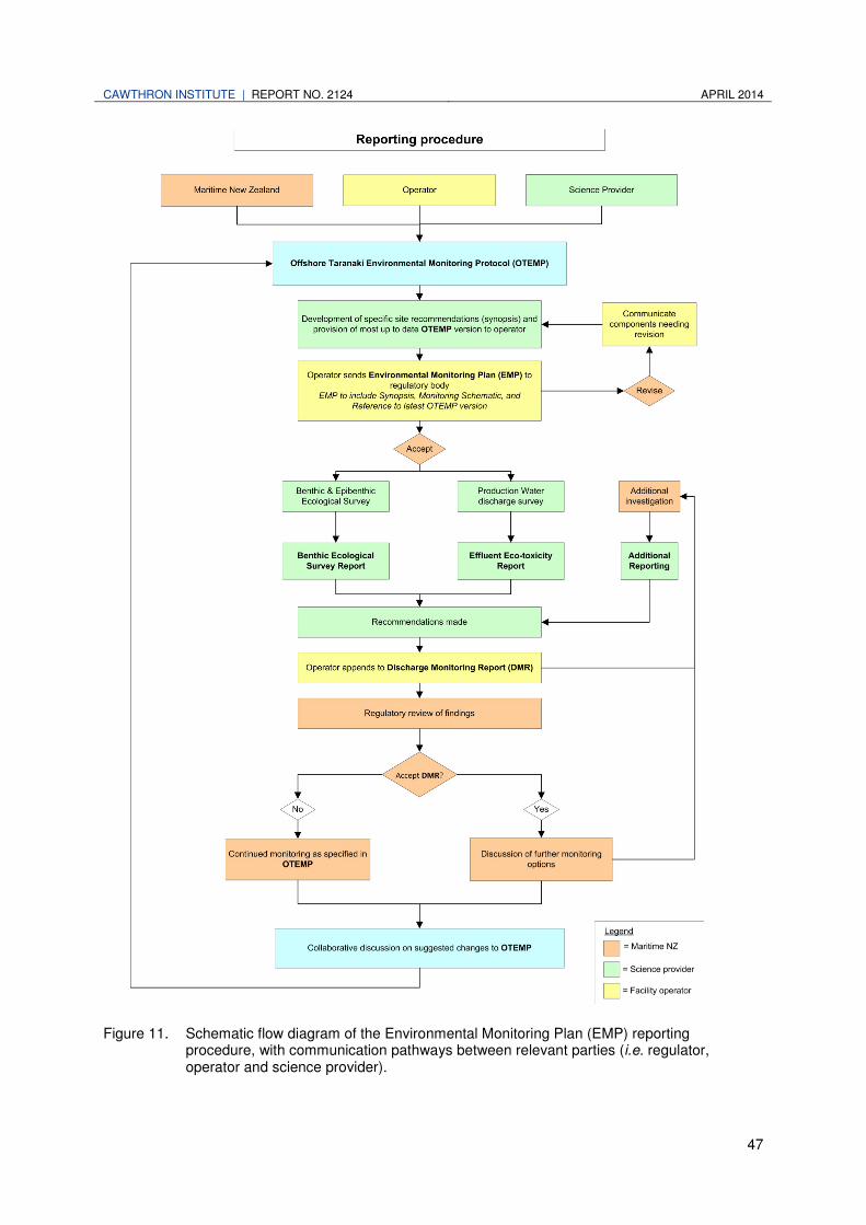
CAWTHRON INSTITUTE | REPORT NO. 2124 APRIL 2014
47
Figure 11. Schematic flow diagram of the Environmental Monitoring Plan (EMP) reporting
procedure, with communication pathways between relevant parties (i.e. regulator, operator and science provider).

APRIL 2014 REPORT NO. 2124 | CAWTHRON INSTITUTE
48
7. FURTHER CONSIDERATIONS
7.1. Developing clear monitoring processes
One suggestion is the development of guidelines and ecological thresholds for
operators to aim for, in order to protect the Taranaki offshore ecosystems. Without
these components, monitoring programmes are at risk of being only an information
gathering exercise, rather than a safeguard.
As yet there are no clear ecological monitoring thresholds specified in the current
Marine Protection Rules (MTA 1994; MPR 2011) or the newly accepted Exclusive
Economic Zone and Continental Shelf (Environmental Effects) Act (EEZ Act 2012).
The EEZ Act (2012) stipulates that all exploration, production and decommissioning
for oil and gas and seabed minerals would require a marine consent from the
Environmental Protection Authority (EPA). This means that operators of offshore
installations in the EEZ and continental shelf are likely to need the following approved,
before the proposed operations can commence:
1. Marine consent for proposed activities (EPA; EEZ Act)
2. Discharge Management Plan relating to oil spill management / planning etc.
(MNZ; MTA 1994)
3. Environmental Monitoring Plan28 for monitoring the environmental effects of
discharges (EPA; EEZ Act).
The transfer of responsibilities from MNZ to the EPA is expected to take some time.
Pending the EEZ Act, MNZ will continue to regulate offshore installation-related
discharges using the Part 200; Marine Protection Rules (MPR 2011), under the
Maritime Transport Act (MTA 1994).
It is suggested that the Resource Management Act (RMA 1991) is used as a
benchmark for ecological and economic sustainability for monitoring guidance in the
interim. Although not legally applicable outside of the 12-mile zone, the RMA (1991)
states that the activity must, “remove, remedy or mitigate any harmful ecological
effects,” rather than solely detecting “marine environmental impacts resulting from
discharges from the installation” (MPR 2011). Using the EEZ (2012), the RMA (1991)
and MPR (2011) together as guidelines, it is recommended the following steps are
taken for discharge-related monitoring:
1. Development of robust Environmental Impact Assessments (EIA) relating to
discharges, with a framework for significance of predictions and scale of effects as
specified in the interim voluntary measures summarised in the Impact Assessment
Guide (EPA 2012).
28
Previously part of the overall DMP document to MNZ.
CAWTHRON INSTITUTE | REPORT NO. 2124 APRIL 2014
49
2. Determine the required sensitivity for sampling techniques (e.g. power analysis,
pilot studies etc.).
3. Development of robust Environmental Monitoring Plans (EMP), which incorporates
predictions / hypotheses from the EIA. Giving monitoring a defined purpose; to
determine whether project activities are resulting in the predicted environmental
effects. Rejecting the monitoring hypotheses could then trigger adaptive
management measures to a level that can “remove, remedy or mitigate any
harmful ecological effects,” (RMA 1991).
By using the recommendations and processes listed above, ecological monitoring in
offshore Taranaki could align with current international standards and effectively
safeguard the marine environment.
7.2. Collective responsibilities
While individual operator ecological monitoring requirements could be met using the
OTEMP, there remains the need for an overarching regional monitoring plan for oil
and gas operators across the offshore Taranaki region. Internationally,
comprehensive regional monitoring programmes investigate regional effects on water
quality and other environmental components such as seabirds, fish and marine
mammals. These regional assessments look at the cumulative impacts of the
installations, and include whether or not valued environmental components interact
with the projects. These components include fish, fish habitat, marine birds and
marine mammals. Project effects on each valued environmental component can be
considered relative to the magnitude, geographic extent, frequency and reversibility of
likely effects. Water quality near discharge points can also be monitored to validate
model predictions on the distribution of produced waters. While these wider regional
components are not directly associated with a specific facilities EMP, it is highly
recommended to pool resources between industry and regulators in the Taranaki
region, to assess the potential of cumulative impacts in the region.
Method validation studies for all past and current monitoring techniques are highly
recommended. Results will provide a better understanding of the comparability of
differing methods and the value and comparability of the historic data sets (e.g. ROV
and single van Veen grab collection methods could be compared with double van
Veen methods). To address this, a joint operator pilot study for method validation
could be run concurrently with offshore Taranaki seabed monitoring programmes. If
implemented, the experimental programme design for a validation study will be
defined separately in a revised joint operator experimental programme.
There is potentially a vast amount of information on the offshore Taranaki region
(ranging from historic well site locations, geological records, as well as past
exploratory and production-related monitoring programmes). As part of the

APRIL 2014 REPORT NO. 2124 | CAWTHRON INSTITUTE
50
developing regulatory framework, it is expected that all operators will be required to
publicise and amalgamate all available information. Retaining such information will be
invaluable to future ecological monitoring in the offshore Taranaki region. For
example, the 2012 North Control site was found to have some sediment
contamination (i.e. elevated levels of mercury). This information becomes highly
relevant for any party who seeks to use (or avoid) this location in the future, as they
would be aware of its background characteristics. Above all, with greater
transparency in monitoring processes, and more publically available information,
informed decisions can be made to better manage offshore activities.

CAWTHRON INSTITUTE | REPORT NO. 2124 APRIL 2014
51
8. REFERENCES
Beauford J, D’Archino R, MacDiarmid A 2009. Mapping the values of New Zealand’s
coastal waters: 4. A Meta-analysis of environmental values. Biosecurity New
Zealand Technical Paper No: 2010 / 08. Prepared for MAFBNZ Policy and Risk
Directorate. 78.
Bothner M, Rendigs R, Campbell E, Doughton M, Parmenter C, O’Dell C, Dilisio G,
Johnson R, Gillison J, Rait N 1985. The Georges Bank monitoring program:
analysis of trace metals in bottom sediments during the third year of
monitoring. Final report submitted to the U.S. MMS, U.S. DOI, USGS, Woods
Holes, MA. 99 pp.
Chapman P 1990. The sediment quality triad approach to determining pollution-
induced degradation. Science of the Total Environment 97: 815-825.
Clarke KR, Warwick RM 1994. Change in marine communities: An approach to
statistical analysis and interpretation. Plymouth Marine Laboratory, UK.
Clarke KR, Gorley RN 2001. PRIMER v5: User manual tutorial. Plymouth Marine
Laboratory, UK.
CM 2010. New Zealand Petroleum Basins. Published by Crown Minerals, Ministry of
Economic Development, PO Box 1473, Wellington 6140, New Zealand. 110 p.
EEZ 2012. Exclusive Economic Zone and Continental Shelf (Environmental Effects)
Bill (321-2). Government Bill as reported from the Local Government and
Environment Committee on 15 May 2012. 136.
Ellis J, Schneider D 1997. Evaluation of a gradient sampling design for environmental
impact assessment. Environmental Monitoring and Assessment. 48 (2): 157-
172.
Ellis J, Fraser G, Russell J 2012. Discharged drilling waste from oil and gas platforms
and its effects on benthic communities. Marine Ecology Progress Series 456:
285–302.
Elvines D, Johnston O, Forrest R, Allen C 2013. Method validation between two grab
sampling techniques, offshore Taranaki. Prepared for AWE Ltd, OMV Ltd, and
STOS Ltd. Cawthron Report No. 2337. 12 p. plus appendices.
EPA 2012. Environmental Protection Authority and the Ministry for the Environment;
Impact Assessment Guide. 1 p.
Forrest R, Johnston O 2011. Post-installation benthic survey of the subtidal
communities and sediments in the vicinity of the Kupe pipeline. Prepared for
Seaworks Ltd and Origin Energy Resources (Kupe) Limited) Cawthron Report
No. 1944. 13.
GNS 2012. Institute of Geological and Nuclear Sciences Ltd (GNS). PDQ maps.
http://maps.gns.cri.nz/website/PDQmap/viewer.htm [accessed July 2012]

APRIL 2014 REPORT NO. 2124 | CAWTHRON INSTITUTE
52
Gray J, Clarke K, Warwick R, Hobbs G 1990. Detection of initial effects of pollution on
marine benthos: an example from the Ekofisk and Eldfisk oilfields, North Sea
Marine Ecological Progress Series 66: 285-299.
Husky-Energy 2004. White Rose Environmental Effects Monitoring Program.
Prepared by Jacques Whitford Environment Limited for Petro-Canada, St.
John’s, NL. 117 p.
Husky-Energy 2006. White Rose Environmental Effects Monitoring Program: 2006:
Volume 1. Prepared by Jacques Whitford Limited. Report No. WR-HSE-RP-
0157 221 p.
IAEA 2003. Collection and preparation of bottom sediment samples for analysis of
radionuclides and trace elements. Prepared for International Atomic Energy
Agency; Nutritional and Health-Related Environmental Studies Section 130 p.
Jogensen L, Renaud P, Cochrane S 2011. Improving benthic monitoring by combining
trawl and grab surveys. Marine Pollution Bulletin 62: 1183-1190.
Johnston O 2011. Baseline benthic survey for the Ruru exploratory well. Prepared for
Shell Todd Oil Services Ltd. Cawthron Report 1939. 22p. plus appendices.
Johnston O, Forrest R 2011. Benthic survey for the Maui-B production platform.
Prepared for Shell Todd Oil Services Ltd. Cawthron Report No. 2036. 30p.
Johnston O, Forrest R 2012a. Benthic ecological survey for the Maari floating
production, storage and off-loading (FPSO) installation and production platform
2012. Prepared for OMV Ltd. Cawthron Report 2126. 39p. plus appendices.
Johnston O, Forrest R 2012b. Benthic ecological survey for the Maui-A platform
drilling programme activities 2012. Prepared for Shell Todd Oil Services Ltd.
Cawthron Report 2125. 41 p. plus appendices.
Johnston O, Forrest R 2012c. Benthic ecological survey for the Tui Umuroa floating
production, storage and off-loading (FPSO) installation 2012. Cawthron Report
2127.
Melton H, Smith J, Martin C, Nedwed T, Mairs H, Raught D 2000. Offshore discharge
of drilling fluids and cuttings — A scientific perspective on public policy. In Rio
Oil and Gas Expo and Conference, Rio de Janeiro, Brazil, 16-19 October 2000.
pp 13.
Middleditch B 1984. Ecological Effects of Produced Water Effluents from Offshore Oil
and Gas Production Platforms.
MPR 2011. Marine Protection Rules: Part 200 – Offshore Installations – Discharges.
As part of the Maritime Transport Act 1994. Eds. Maritime New Zealand
Consolidation, 1 Janurary 2011. P.O. Box 27006, Wellington 6141, New
Zealand. 27 p.
MTA 1994. Martime Transport Act 1994. Public Act 1994, No 104. Date of assent 17
November 1994. Act administered by the Ministry of Transport. pp 368.
CAWTHRON INSTITUTE | REPORT NO. 2124 APRIL 2014
53
Neff J, Bothner M, Maciolek N, Grassle J 1989. Impacts of exploratory drilling for oil
and gas on the benthic environment of Georges Bank. Mar Environ Res 27:
77-114.
Neff J, Lee K, DeBlois E 2011. Produced Water: Chapter 1, Produced Water:
Overview of Composition, Fates, and Effects. Eds; Lee, K and Neff, J. Springer
Science & Business Media, LLC 2011.
Neff JM, McKelvie S, Ayers RC 2000. Environmental impacts of synthetic based
drilling fluids. Report prepared for MMS by Robert Ayers & Associates, Inc.
August 2000. U.S. Department of the Interior, Minerals Management Service,
Gulf of Mexico OCS Region, New Orleans, LA. OCS Study MMS 2000-064.
118 pp.
OECD 1995. Organisation for Economic Co-operation and Development. Guidance
Document for Aquatic Effects Assessment. Paris. OECD Environment
Monographs, Paris No. 92.
Patin S 1999. Environmental Impact of the Offshore Oil and Gas Industry; Chapter 7;
Ecological and Fisheries Implications. EcoMonitoring Publishing, P.O. Box 866,
East Northport, NY, USA. 401 p.
Petro-Canada 2007. Terra Nova Environmental Effects Monitoring Program. Year 5.
Prepared by Jacques Whitford Environment Limited for Petro-Canada, St. JW
Job No: 1014454 236 p.
Ray J, Ranier-Engelhardt F 1992. Produced water: technological / environmental
issues and solutions. Environmental Science Research 46.
RMA 1991. Resource Management Act; New Zealand Public Act No: 69. Ministry for
the Environment.
Rutherford K, Zuur B, Race P 1994. Resource Management Ideas: No. 10:
"Reasonable Mixing" A discussion of reasonable mixing in water quality
management: 15 p.
Sneddon R 2011. Assessment of Effects on Benthic Habitats from Exploratory Well
Drilling at the Tuatara Rig Site Outer Tasman Bay: 2010 Post-Drilling Survey.
Prepared for AWE NZ. Cawthron Report No. 1892. 20p. plus appendices.
US.EPA 2002. Methods for Measuring the Acute Toxicity of Effluents and Receiving
Waters to Freshwater and Marine Organisms. EPA-821-R-02-012. Fifth
Edition. 275 p.

CAWTHRON INSTITUTE | REPORT NO. 2124 APRIL 2014
54
9. APPENDICES
Appendix 1. Schematic flow diagram of the proposed Offshore Taranaki Environmental Monitoring Protocol (OTEMP) components and processes.

CAWTHRON INSTITUTE | REPORT NO. 2124 APRIL 2014
55
Appendix 2. Environmental Monitoring Plan (EMP) guideline documents.
ANZECC 2000
The ANZECC (2000) guidelines are recommended to be used as the most recent
guidelines for assessing sediment contamination in marine / aquatic monitoring based
scenarios. Table 3.4.1 of the ANZECC 2000 guidelines illustrates the process of
decision-making, using a host of trigger values and ecosystem condition levels to help
ascertain the level of risk associated with the proposed activity (in this case drilling).
ANZECC 2000 updates the 1992 ANZECC Water Quality Guidelines and has been
modified to take the New Zealand context into consideration.
The guidelines provide contaminant chemical and physical trigger values, condition
indicators and performance indicators. In terms of the Umuroa EMP, the ANZECC
(2000) guidelines are recommended to be referred to for trigger values pertaining to
chemical sediment contamination and to provide a means to ascertain the potential for
significant ecological change in the associated offshore benthic environment. The
most appropriate ANZECC (2000) trigger value scenario is considered to be an 80-
95% (species) level of protection for slightly - moderately disturbed environments.
This consideration is due to the overall Taranaki Bight offshore region being described
by Biosecurity New Zealand (Beaumont et al. 2010) as being an area that stood out
as having a comparatively uniform physical environment, and was judged to be of
relatively low importance with respect to both habitat and biological diversity based on
the Marine Environmental Classification (MEC) system.
Puget Sound Protocol (PSEP 1987)
The United States Environmental Protection Agency (USEPA) developed the
Recommended Protocols for sampling and analysing subtidal benthic
macroinvertebrate assemblages in Puget Sound (PSEP 1987; Puget Sound Estuary
Protocol). Although specific to the Puget Sound, the protocols have become a
worldwide standard for conducting subtidal benthic monitoring programmes, baseline
surveys, and investigations. The use of standardised methodology helps data sets to
be directly comparable and enables data to be integrated into regional, nationwide,
and world wide databases. PSEP (1987) has been used to provide some guidance for
benthic related field work and analyses associated specifically with van Veen grab
sampling, and macrofaunal sampling.
Ellis et al. (2012)
Guidance for oil field related benthic sampling programmes was provided from the
Ellis et al. (2012) review paper; “Effects on benthic communities of drilling water from
marine exploration and production platforms” (has been submitted and accepted for
publication in the Marine Ecology Progress Series Journal). As a result of this review,
an industry standard can now be recommended by Cawthron, which will relate to the
majority of offshore oil industry benthic sampling programmes.

APRIL 2014 REPORT NO. 2124 | CAWTHRON INSTITUTE
56
Kingsford and Battershill 1998
New Zealand’s Department of Conservation and the National Institute of Water and
Atmospheric Research (NIWA) developed the reference book for “studying temperate
marine environments – A hand book for ecologists”. This reference provides a
combination of technical and practical information relative to the study of temperate
marine environments and provides guidance on appropriate statistical analyses,
specific taxonomist names and contact details and guidance on the treatment and
identification of specimens.

CAWTHRON INSTITUTE | REPORT NO. 2124 APRIL 2014
57
Appendix 3. The MetOcean Solutions Ltd (MSL) implementation of the Princeton Ocean Model (POM) for hindcasting the depth-averaged wind-driven and tidal currents.
The near-surface and depth-averaged current regime has been derived from a 12-
year current hindcast, using a two stage modelling approach. The first stage simulates
the spatial depth-averaged current field, while the second stage applies a vertical
profile model to derive the depth specific currents velocities. The MetOcean Solutions
Ltd (MSL) implementation of POM (Princeton Ocean Model) was used to hindcast the
depth-averaged wind-driven and tidal currents. POM is a primitive equation ocean
model that numerically solves for oceanic current motions, and is used worldwide in
numerous scientific applications studying oceanic and shelf circulation. For model
equations and methods refer to MetOcean Solutions Ltd.
Model equations
For the hindcast simulations, MSL-POM is used in a vertically integrated two-
dimensional mode, solving the momentum and mass conservation equations given
by:
hhy
u
x
uA
x
P
xgfv
y
uv
x
uu
t
ux
b
x
w
H
a
ρ
τ
ρ
τ
ρ
η−+
∂
∂+
∂
∂+
∂
∂−
∂
∂−=−
∂
∂+
∂
∂+
∂
∂2
2
2
21
hhy
v
x
vA
y
P
ygfv
y
vv
x
vu
t
vy
b
y
w
H
a
ρ
τ
ρ
τ
ρ
η−+
∂
∂+
∂
∂+
∂
∂−
∂
∂−=−
∂
∂+
∂
∂+
∂
∂2
2
2
21
(1 a,b,c)
where t is the time, u and v are the depth-averaged velocities in the x and y directions
respectively, h the depth, η is the elevation of the surface, g the gravitational
acceleration, f the Coriolis parameter, ρ the density of water, and Pa is atmospheric
pressure.
AH is a horizontal eddy viscosity coefficient, calculated with a Smagorinsky
parameterisation,
2
1
222
2
1
∂
∂+
∂
∂+
∂
∂+
∂
∂∆∆=
y
v
y
u
x
v
x
uyxCA mH (2)
with Cm set at 0.2.
The surface and bottom shear stress, τw and τb are due to wind and bottom friction.
The bed shear stress is parameterised with a quadratic type friction law,
( ) ( )vvuCuvuC D
y
bD
x
b
2222 +=+= ττ (3 a,b)
that depends on an adjustable drag coefficient, CD ~ 10-3
[ ]( ) [ ]( )0=
∂
+∂+
∂
+∂+
∂
∂
y
hv
x
hu
t
ηηη
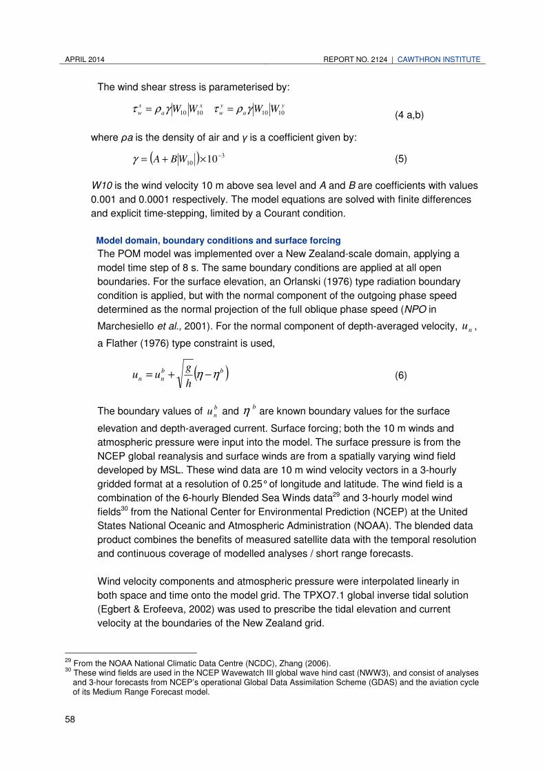
APRIL 2014 REPORT NO. 2124 | CAWTHRON INSTITUTE
58
The wind shear stress is parameterised by:
(4 a,b)
where ρa is the density of air and γ is a coefficient given by:
( ) 3
10 10−×+= WBAγ (5)
W10 is the wind velocity 10 m above sea level and A and B are coefficients with values
0.001 and 0.0001 respectively. The model equations are solved with finite differences
and explicit time-stepping, limited by a Courant condition.
Model domain, boundary conditions and surface forcing
The POM model was implemented over a New Zealand-scale domain, applying a
model time step of 8 s. The same boundary conditions are applied at all open
boundaries. For the surface elevation, an Orlanski (1976) type radiation boundary
condition is applied, but with the normal component of the outgoing phase speed
determined as the normal projection of the full oblique phase speed (NPO in
Marchesiello et al., 2001). For the normal component of depth-averaged velocity, nu ,
a Flather (1976) type constraint is used,
( )bb
nnh
guu ηη −+= (6)
The boundary values of b
nu and bη are known boundary values for the surface
elevation and depth-averaged current. Surface forcing; both the 10 m winds and
atmospheric pressure were input into the model. The surface pressure is from the
NCEP global reanalysis and surface winds are from a spatially varying wind field
developed by MSL. These wind data are 10 m wind velocity vectors in a 3-hourly
gridded format at a resolution of 0.25° of longitude and latitude. The wind field is a
combination of the 6-hourly Blended Sea Winds data29 and 3-hourly model wind
fields30 from the National Center for Environmental Prediction (NCEP) at the United
States National Oceanic and Atmospheric Administration (NOAA). The blended data
product combines the benefits of measured satellite data with the temporal resolution
and continuous coverage of modelled analyses / short range forecasts.
Wind velocity components and atmospheric pressure were interpolated linearly in
both space and time onto the model grid. The TPXO7.1 global inverse tidal solution
(Egbert & Erofeeva, 2002) was used to prescribe the tidal elevation and current
velocity at the boundaries of the New Zealand grid.
29
From the NOAA National Climatic Data Centre (NCDC), Zhang (2006). 30
These wind fields are used in the NCEP Wavewatch III global wave hind cast (NWW3), and consist of analyses and 3-hour forecasts from NCEP’s operational Global Data Assimilation Scheme (GDAS) and the aviation cycle of its Medium Range Forecast model.
y
a
y
w
x
a
x
w WWWW 10101010 γρτγρτ ==

CAWTHRON INSTITUTE | REPORT NO. 2124 APRIL 2014
59
Model output
The 2-D hydrodynamic model was used to hindcast the period 1998-2009. Depth-
averaged currents were extracted for the hindcast period at 3-hourly intervals. To
interpolate the 3-hourly depth-averaged currents to smaller time steps used in the
vertical profile model, a combined tidal / residual method was used. Harmonic
analysis was applied to the full 3-hourly model time series to derive the tidal
constituents of the current. The tidal contribution is then calculated and subtracted
from the raw model output to leave a slowly varying residual flow. For a given time the
total flow is then reconstructed from the tidal signal calculated from the constituents
and the residual component calculated by cubic interpolation from the 3-hour residual
time series.
Current profile model
The time series of depth-averaged flow at the site was post-processed to calculate
depth variation of the currents and derive near surface and near bed flow velocities. A
one-dimensional model of the vertical profile was used to recover depth variation
caused by Ekman veering and bed friction. The one-dimensional model solves for the
departure of the current velocity at a particular depth from the depth-averaged value
calculated in the 2-D model. For a total velocity u~ at depth z (measured upwards)
given by:
∫ =′′+=h
dzuzuuzu0
0)()(~ (7)
The velocity departure from the depth averaged value is calculated from the
equations:
hhz
vA
zuf
t
v
hhz
uA
zvf
t
u
y
bv
y
w
z
x
bv
x
w
z
ρ
τ
ρ
τ
ρ
τ
ρ
τ
+−∂
′∂
∂
∂=′+
∂
′∂
+−∂
′∂
∂
∂=′−
∂
′∂
(8 a,b)
These equations are derived by subtracting the depth-averaged equations from the
full 3-D equations. Nonlinear terms involving u′ and baroclinic terms are neglected.
The boundary conditions are:
hz
vA
hz
uA
y
w
z
x
w
zρ
τ
ρ
τ=
∂
′∂=
∂
′∂; (9 a,b)
at the surface and,
hz
vA
hz
uA
y
bv
z
x
bv
zρ
τ
ρ
τ−=
∂
′∂−=
∂
′∂; (10 a,b)
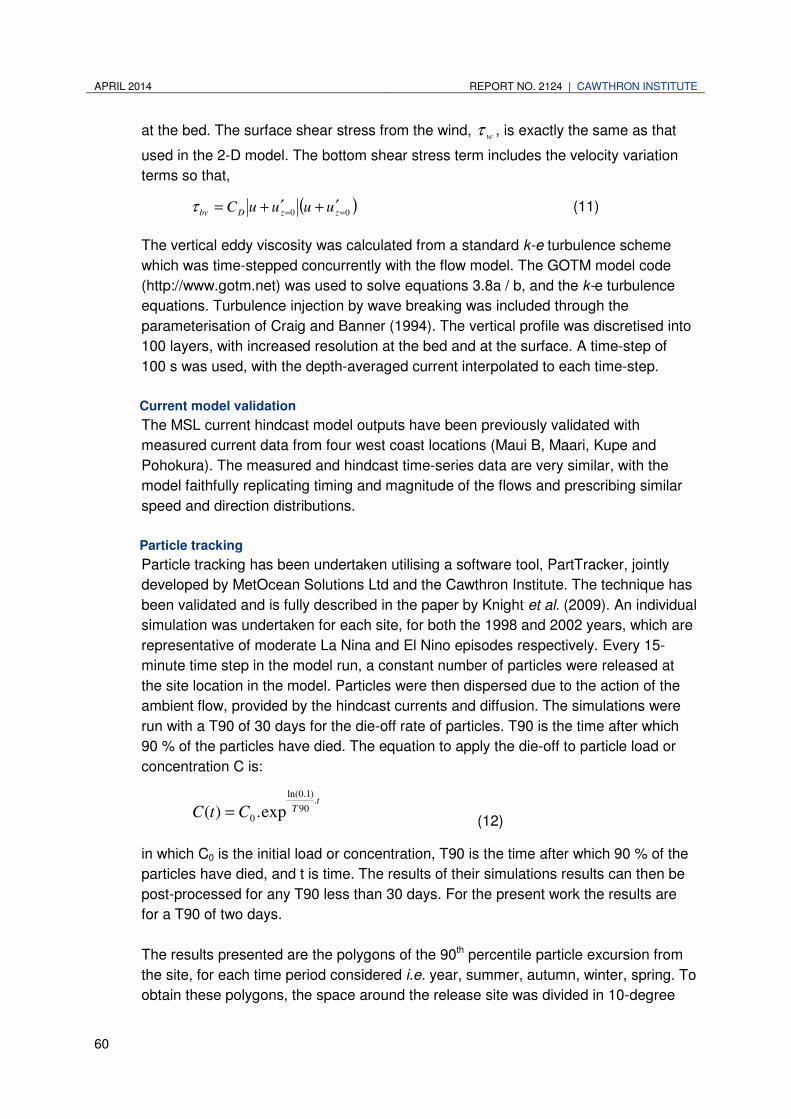
APRIL 2014 REPORT NO. 2124 | CAWTHRON INSTITUTE
60
at the bed. The surface shear stress from the wind, wτ , is exactly the same as that
used in the 2-D model. The bottom shear stress term includes the velocity variation
terms so that,
( )00 ==′+′+= zzDbv uuuuCτ (11)
The vertical eddy viscosity was calculated from a standard k-e turbulence scheme
which was time-stepped concurrently with the flow model. The GOTM model code
(http://www.gotm.net) was used to solve equations 3.8a / b, and the k-e turbulence
equations. Turbulence injection by wave breaking was included through the
parameterisation of Craig and Banner (1994). The vertical profile was discretised into
100 layers, with increased resolution at the bed and at the surface. A time-step of
100 s was used, with the depth-averaged current interpolated to each time-step.
Current model validation
The MSL current hindcast model outputs have been previously validated with
measured current data from four west coast locations (Maui B, Maari, Kupe and
Pohokura). The measured and hindcast time-series data are very similar, with the
model faithfully replicating timing and magnitude of the flows and prescribing similar
speed and direction distributions.
Particle tracking
Particle tracking has been undertaken utilising a software tool, PartTracker, jointly
developed by MetOcean Solutions Ltd and the Cawthron Institute. The technique has
been validated and is fully described in the paper by Knight et al. (2009). An individual
simulation was undertaken for each site, for both the 1998 and 2002 years, which are
representative of moderate La Nina and El Nino episodes respectively. Every 15-
minute time step in the model run, a constant number of particles were released at
the site location in the model. Particles were then dispersed due to the action of the
ambient flow, provided by the hindcast currents and diffusion. The simulations were
run with a T90 of 30 days for the die-off rate of particles. T90 is the time after which
90 % of the particles have died. The equation to apply the die-off to particle load or
concentration C is:
tTCtC
.90
)1.0ln(
0 exp.)( = (12)
in which C0 is the initial load or concentration, T90 is the time after which 90 % of the
particles have died, and t is time. The results of their simulations results can then be
post-processed for any T90 less than 30 days. For the present work the results are
for a T90 of two days.
The results presented are the polygons of the 90th percentile particle excursion from
the site, for each time period considered i.e. year, summer, autumn, winter, spring. To
obtain these polygons, the space around the release site was divided in 10-degree

CAWTHRON INSTITUTE | REPORT NO. 2124 APRIL 2014
61
wide directional bin. For a given period of time, all particles within that bin were
identified and their distance from the release site computed. The 90th percentile of
these distances provides a polygon point.
References cited in Appendix 2
Egbert G, Erofeeva L 2002. Efficient inverse modelling of barotropic ocean tides.
Journal of Atmospheric and Oceanic Technology, 19, N2
Flather RA 1976. A tidal model of the northwest European continental shelf. Memoires
de la Societe Royale des Sciences de Liege 6 (10), 141-164
Knight BR; Zyngfogel R, Forrest B 2009. PartTracker – a fate analysis tool for marine
particles. In Proceedings of Australasian Coasts and Ports Conference 2009.
Dawe I, Ed. New Zealand Coastal Society, Wellington. pp 8
Marchesiello P, Mc Williams JC, Shchepetkin A 2001. Open boundary conditions for
the long-term integration of regional oceanic models. Ocean Modelling, 3, 1-20
Mellor GL 2004. Users guide for “A three-dimensional, primitive equation, numerical
ocean model”. Princeton University, Princeton, NJ. Available from:
http://www.aos.princeton.edu/WWPUBLIC/htdocs.pom/
Orlanski I 1976. A simple boundary condition for unbounded hyperbolic flows. Journal
of Computational Physics 21, 251-269.

APRIL 2014 REPORT NO. 2124 | CAWTHRON INSTITUTE
62
Appendix 4. A generic example of an Environmental Monitoring Plan (EMP) as it might be used in conjunction with the Offshore Taranaki Environmental Monitoring Protocol (OTEMP), including the site-specific synopsis (table below), deposition modelling, and area map showing location of the operation and the proposed sampling locations (Figure A4.1). Note that this is a general guide only, and this particular example is of an exploratory synopsis. Production-related synopses will vary slightly.
Summary
This synopsis details an exploratory drill project proposed by ABC Ltd. for the proposed ‘Noname’ exploration drilling well site. This synopsis covers the general approach and methodology for the Environmental Monitoring Plan (EMP) including station locations, frequency of sampling, and general reporting framework but is in no way intended to function as the full monitoring plan.
Operator ABC Ltd. New Zealand
Facility Noname exploration well site; Drilling rig [Insert name]
Field schedule Winter 2013; Winter 2014
Methodology As recommended by OTEMP (2012)
Double van Veen grab (benthic): Infauna, sediment characteristics (including incidental observations) and chemistry
Video sled (epibenthic): Qualitative observations of seafloor, biota, biogenic structures, and incidental observations.
Sampling stations As recommended by OTEMP (2012)
Benthic: 18 at proposed drill site and three at the Control site (Figure A4.1, allocated according to flow modelling shown in Figure A4.2)
Epibenthic: Four at the proposed drill site and two at the Control site
Sampling
frequency
The pre- and post-drill surveys to be carried out within a 12-month
period, and drilling operations will be undertaken at any time between
the surveys (OTEMP 2012).
Reporting
frequency
Within six months of field effort. Subsequent reports will include
analyses from previous sampling efforts and be to a standard
appropriate for external peer review. All raw data will be included in the
report(s) or available on request.
Test hypotheses • H0.1: There will be no effects to the physical sediment
characteristics (grain-size and AFDW), as a result of the drilling
activity.
• H0.2: Project discharges will not result in sediment chemistry
concentrations to exceed ISQG-Low guideline values (where
applicable) or be significantly higher than background/control
concentrations
• H0.3: Project discharges will not cause biological effects
• H0.4: Incidental observations of project related debris will not be
observed
Exclusion zone No exclusion zone applies as there are no confounding structures
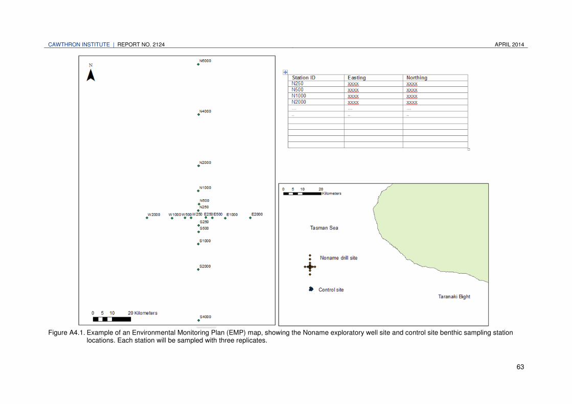
CAWTHRON INSTITUTE | REPORT NO. 2124 APRIL 2014
63
Figure A4.1. Example of an Environmental Monitoring Plan (EMP) map, showing the Noname exploratory well site and control site benthic sampling station
locations. Each station will be sampled with three replicates.

APRIL 2014 REPORT NO. 2124 | CAWTHRON INSTITUTE
64
Figure A4.2. Sampling stations at the Noname exploratory well site showing discharge flow model
results.

CAWTHRON INSTITUTE | REPORT NO. 2124 APRIL 2014
65
Appendix 5. Rationale for each sampling method.
The following sections describe the rationale used to verify that the sampling
procedures employed for water and benthic / sediment quality sampling employed in
this OTEMP are appropriate.
Benthic / sediment sampling method validation
Previous surveys in the Taranaki region have used a variety of different methods and
approaches including remotely operated vehicle (ROV) core samples. The OTEMP
approach uses whole van Veen sediment grabs, and while this is internationally
consistent, it is not known to have been used previously in the region.
The full van Veen grab sampling method has been validated in terms of sensitivity to
detect change in macrofaunal assemblages, sediment chemistry and sediment
characteristics. Using the full-grab sampling method throughout summer 2012,
regional monitoring results showed high abundances, distinct macrofaunal groupings,
relationships with sediment characteristics, and spatial variation. With such distinct
patterns in results, it is assumed that the full grab method is adequately sensitive for
the purpose of Taranaki environmental monitoring.
To date, one Taranaki offshore specific method validation study has been completed;
the study, by Elvines et al. (2013), compared single and double van Veen grab
macrofaunal results. Results from the study provided a means of comparing data from
the two methods of grab sampling. Ideally, the previously collected ROV and other
data (e.g. other grab collection methods) could also be incorporated to some extent,
but this would involve further validation sampling in order to compare the different
methodologies historically employed.
Epibenthic sampling method selection
Epibenthic fauna, sometimes missed by benthic grab sampling, are reported to have
ecological functions that differ to that obtained by benthic grabs
(Jogensen et al. 2011). These epifaunal (epibenthic) and infaunal (benthic)
communities may also be expected to respond differently to human induced stressors.
Therefore, in order to assess the full health of both components of the benthic
community, and to provide a more sensitive monitoring technique, a combined
epibenthic and benthic type monitoring programme is recommended.
The epifaunal analysis is not intended to be fully quantitative or exact, although it does
provide an approximate ‘snap shot’ of the biota living on the surface of the soft
sediments (semi-quantitative at best). If this remains the primary objective for
epibenthic sampling, then no method validation study is considered necessary to
determine appropriate sample size or replication.

APRIL 2014 REPORT NO. 2124 | CAWTHRON INSTITUTE
66
There may also be occasions where epibenthic video footage can be obtained
concurrently with ROV subsea surveys. These surveys are undertaken at all of the
fields on an annual or bi-annual (two yearly) basis. Therefore, if no video footage of
the seabed is obtained during specific sampling surveys, then there is potential to
obtain some opportunistically.
Direct toxicity assessment method selection: production-related discharges
A direct toxicity assessment (DTA) is a series of bioassays which test varying dilutions
of the actual effluent on a number of different organisms to monitor their response.
While individual constituents of effluent may not necessarily produce an ecotoxic
effect these individual effluent components may produce toxic effects from their
interaction in the effluent stream, and it is the detection of these synergistic effects
that is the primary intention of this DTA testing.
Because different species have variable sensitivity to contaminants depending on
their taxa and life-stages, testing the toxicity of potentially contaminated discharges
(e.g. produced water) using DTA should be undertaken using a range of model
organisms, selected to represent relevant trophic levels present in the receiving
ecosystem. Standard methodologies using relevant local species have been
developed in many countries31 and most include algae, invertebrates and fish. The
underlying purpose of using multiple species in the suggested DTA testing will be to
identify that which is most sensitive, providing a conservative ecological indicator and
presenting the option of using this species for setting protective discharge limits32.
While DTA assesses the general toxicity of discharge to biota, there are associated
limitations. DTA alone cannot identify specific toxic components of an effluent;
however, if toxicity is detected (over a specified threshold) separate compositional
studies can help determine discharge constituents, which can then be individually
tested using DTA, thus determining the toxic component(s) of the discharge. If the
toxic effect is a produced by the interaction of two or more of the components, this is
more difficult to establish. Single DTA toxicity results are also limited to one-off
samples that may not necessarily be representative of temporal variability of the
effluent. This limitation can be overcome by adopting multiple or continuous sampling
over time.
If testing multiple or continuous samples is not feasible, single discharge samples can
be taken yearly, preferably at the same time of year and when the most contaminated,
highest volume of discharge is predicted (to provide a worst-case discharge scenario).
The efficacy / validity of an annual sampling technique should be evaluated
throughout the independently assessed report stages. It is suggested that each
31
The profile generated by the results of those tests can also be used to assess the potential impacts of an effluent.
32 The earliest life-stages and any particular species which tend to be most sensitive are therefore likely to provide the highest level of protection.
CAWTHRON INSTITUTE | REPORT NO. 2124 APRIL 2014
67
individual bioassay, as well as an overall summary including any recommendations,
are included in the DTA reports.
Dispersion modelling validation
While dispersion modelling is often done separately as part of the EIA associated with
drilling or production activities, it is included in this section as it is an important
component of determining appropriate benthic sampling station locations for
monitoring plans. A process similar to the MetOcean Solutions Ltd (MSL)
implementation of Princeton Ocean Model (POM), should be used to hindcast the
depth-averaged wind-driven and tidal currents (as specified in Appendix 3). POM is a
primitive equation ocean model that numerically solves for oceanic current motions,
and is used internationally in numerous scientific applications in oceanic and shelf
circulation. Within OTEMP, these equations should be used to determine the major
and minor axes of discharge flow, allowing appropriate station allocation (i.e. more
stations on major flow axes), and can potentially be used to predict site-specific spatial
dilution of discharges33.
The MSL current hindcast model outputs have been previously validated with
measured current data from four west coast locations (Maui B, Maari, Kupe and
Pohokura). The measured and hindcast time-series data are very similar, with the
model faithfully replicating timing and magnitude of the flows and prescribing similar
speed and direction distributions.
33
Assuming the discharge behaves similarly to the tracked particles.
Top Related