


Languages
Pages
Legal


R / Bioconductor for ’Omics Analysis
Martin Morgan
Roswell Park Cancer InstituteBuffalo, NY, USA
31 October 2016
R / Bioconductor for ’Omics Analysis 1 / 18

Introduction
https://bioconductor.orghttps://support.bioconductor.org
Analysis and comprehension ofhigh-throughput genomic data.
Started 2002
1295 packages – developed by‘us’ and user-contributed.
Well-used and respected.
43k unique IP downloads /month.
17,000 PubMedCentralcitations.
R / Bioconductor for ’Omics Analysis Introduction 2 / 18

Scope
Based on the R programming language.
Intrinsically statistical nature of data.
Flexible analysis options for new or customized types of analysis.
‘Old-school’ scripts for reproducibility; modern graphical interfaces foreasy use.
Domains of application.
Sequencing: differential expression, ChIP-seq, variants, gene setenrichment, . . .
Microarrays: methylation, expression, copy number, . . .
Flow cytometry, proteomics, . . .
R / Bioconductor for ’Omics Analysis Introduction 3 / 18

Install, learn, use, develop
Install1
R, RStudio,Bioconductor
Learn
Courses, vignettes,workflows
Use
Vignettes, manuals,support site2
Develop
1https://bioconductor.org2https://support.bioconductor.org
R / Bioconductor for ’Omics Analysis Introduction 4 / 18

R : base packages
x <- rnorm(1000)
y <- x + rnorm(1000, sd=.5)
df <- data.frame(X=x, Y=y)
fit <- lm(Y ~ X, df)
anova(fit)
## Analysis of Variance Table
##
## Response: Y
## Df Sum Sq Mean Sq F value Pr(>F)
## X 1 925.99 925.99 3557.7 < 2.2e-16 ***
## Residuals 998 259.76 0.26
## ---
## Signif. codes: 0 '***' 0.001 '**' 0.01 '*' 0.05 '.' 0.1 ' ' 1
R / Bioconductor for ’Omics Analysis Introduction 5 / 18

R : contributed packages
library(ggplot2)
ggplot(df, aes(x=x, y=y)) +
geom_point() +
stat_smooth(method="lm")●
●
●●
●
●
●
●
●
●
●
●
●
●
●
●
●●
●
●
●
●
●
●
●
●
●
●
●
●
●
●
●
●
●
●●
●
●
●
●
●
●
●
●
●
●
●
●●
●
●
●
●
●●
●
●
●
●
●
●
●
●
●
●
●
●
●
●
●
●
●
●
●
●
●
●
●
●
●
●
●
●
●
●
●
●●
●
●
●
●
●
●
●
●
●
●
●
●
●
●●
●
●
●
●
●
●
●
●
●
●
●
●
●
●
●
●
●
●
●●
●
●
●
●
●
●
●
●
●
●
●
●●●
●
●
●●
●
●
●
●
●
●
●
●
●
●
●
●
●
●
●●
●
●
●
●
●
●
●
●
●
●
●
●
●
●
●
●
● ●
●
●
●
●
●
●
●
●
●
●
●
●
●
●
●
●
●
●
●
●
●
●
●
●
●
●
●●
●
●
●
●
●
●
●
●
●
●
●
●
●
●
●
●
●
●
●
●
●
●
●
●
●
●
●
●
●
●
●
●
●
●
●
●
●
●
●
●
●
●
●
●
●
●
●
●
●
●
●
●
●
●
●
●
●
●
●
●
●
●
●●
●
●
●
●
●
●
●
●
●
●
●
●
●
●
●
●
●
●●
●
●
●
●
●
●
●
●
●
●
●
●●
●
●●
●
●
●
●
●
●
●
●
●
●
●
●
●
●
●
●
●
●
●
●
●●
●
●
●
●
●
●
●
●
●●
●
●
●
●
●
●
●
●
●
●
●●
●
●
●
●
●
●●
●
●
●
●
●
●
●
●
●
●
●
●
●
●●
●
●
●
●
●
●
●
●
●
●
●
●
●
●
●
●
●
●
●
●
●
●
●
●
●
●
●
●
●
●
●
●●
●
●
●
●●
●
●
●
●
●
●●
●
●●
●
●
●
●
●
●
●
●
●
●
●
●
●
●
●
●
●
●
●
●
●
●
●
●●
●
●
●
●
●●
●
●
●
●
●
●
●●
● ●
●
●
●
●
●
●
●
●
●
●
● ●●
●
●
●●
●
●
●
●
●
●
●
●
●
●
●
●
●
●
●
●●
●
●
●
●
●
●
●
●
●
●
●
●
●
●
●
●
●
●
●
●
● ●
●
●
●
●
● ●
●
●
●
●
●
●
●
●
●
●
●
●
●
●
●
●
●
●
●
●
●
●
●
●
●
●
●●
●
●
●
●
●
●●
●
●
●
●
●
●
●
●
●
●
●
●●
●
●
●
●
●
●
●
●
●
●
●
●
●
●●
●
●●
●
●
●
●
●
●●
●
●
●
●
●
●
●
●
●
●
●
●
●
●
●
●
●
●
●
●
●
●
●
●
●
●
●
●
●
●
●
●
●
●
●
●
●
●
●
●●
●
●
●
●
●
●
●
●
●
●
●●
●●
●
●
●
●
●
●
●
●
●
●
● ●
●
●
●
●
●
●
●
●
●
●
●
●
●
●
●●
●
●
●
●
●
●
●
●
●
●
● ●
●●
●●
●
●●
●
●
●
●
●
●
●
●
●
●
●
●
●
●
●
●●●
●●
●
●
●
●
●
●
●
●
●
●
●
●
●
●
●
●
●
●
● ●
●
●
●
●
●
●
●
●
●
●
●
●
●
●
●
●
●
●●
●
●●
●
●
●
●
●
●
●
●
●
●
●
●
●
●
●
●
●
●
●
●
●●
●
●
●
●
●●
●
●
●
●
●
●●
●
●
●
●
●
●
●
●
●
●
●
●
●
●
●
●
●
●
●
●
●
●
●
●
●
●
●
●
●
●●
●
●
●
●
● ●
●
●
●
●
●
●
●
●
●
●
●
●
●
●
●
●
●
●
●
●
●
●
●
●
●
●
●
●
●
● ●
●
●
●
●
●
●
●
●
●
●
●
●
●
●● ●
●
●
●
●
●
●
●
●
●
●
●
●
●
●
●
●
●
●
●
●
●
●
●
●
●
●
●
●
●
●
●
●
●
●
●
●
●
●
●
●
●
●
●
●
●
●
●
●
●
●
●
●
●
●
●
●
●
●
●
●
●
●
●
●
●
●
●
●
●
●
●
●
●
●
●
●
●
●
●
●
●
●
●
●
●
●●
●
●
●
●
●
●
●
●
●
●
●
●
●
●
●
●
●
●
●
●
● ●
●
●
●
●
●●
●
●
●
●
●
●
●
●
●
−2
0
2
4
−2 0 2x
y
R / Bioconductor for ’Omics Analysis Introduction 6 / 18
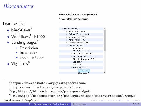
Bioconductor
Learn & use
biocViews3
Workflows4, F1000
Landing pages5
I DescriptionI InstallationI Documentation
Vignettes6
3https://bioconductor.org/packages/release4http://bioconductor.org/help/workflows5e.g., https://bioconductor.org/packages/edgeR6e.g., https://bioconductor.org/packages/release/bioc/vignettes/DESeq2/
inst/doc/DESeq2.pdfR / Bioconductor for ’Omics Analysis Introduction 7 / 18

Bioconductor
Input: description of experimental design and summary of read countsoverlapping regions of interest.
pdata <- read.table("pdata.tab") # Plain text files
assay <- read.table("assay.tab")
library(DESeq2)
dds <- DESeqDataSetFromMatrix(assay, pdata, ~ cell + dex)
result(DESeq(dds))
Output: top table of differentially expressed genes, log fold change,adjusted P-value, etc.
R / Bioconductor for ’Omics Analysis Introduction 8 / 18

A typical work flow: RNA-seq
Research question
Designed experiment
Gene-level differential expression
RNA-seq data
Data processing steps
Quality assessment.
Alignment and summary tocount table.
Assessment of differentialexpression.
Results placed in context, e.g.,gene set enrichment.
http://bio.lundberg.gu.se/
courses/vt13/rnaseq.html
R / Bioconductor for ’Omics Analysis A typical work flow 9 / 18

Pre-processing, alignment
Pre-processing
FASTQ file read quality assessment
Alignment & summary (traditional)
Full alignment to BAM files, summarizing gene or transcriptabundance, e.g., Bowtie / tophat / cufflinks; RSEM; Rsubread
Summarize to gene-level count tables or estimates of abundance
Counts are important: information about statistical uncertainty ofestimate
Alignment & summary (contemporary)
Approximate alignment directly to count tables of transcripts orgenes, e.g., kallisto7, salmon8
7https://pachterlab.github.io/kallisto/8http://salmon.readthedocs.io/en/latest/salmon.html
R / Bioconductor for ’Omics Analysis A typical work flow 10 / 18

Differential expression
E.g., limma, edgeR, DESeq2
library(tximport)
df <- read.table("pdata.tab")
## tx2gene: see tximport vignette
txi <- tximport(df$files, type="kallisto", tx2gene=tx2gene)
library(DESeq2)
dds <- DESeqDataSetFromMatrix(txi, samples, ~ cell + dex)
result(DESeq(dds))
Account for library size differences (normalization)
Apply sophisticated statistical model (negative binomial)
Moderate test statistics (helps with small sample size)
Performant, tested, correct.
R / Bioconductor for ’Omics Analysis A typical work flow 11 / 18

Analysis & comprehension
Annotation packages
Packages, e.g., org.* : symbolmapping; BSgenome.* : genomesequence; TxDb.* : gene models
Query web services, e.g.,biomaRt, uniprot.ws,KEGGREST , . . .
AnnotationHub: consortium andother large-scale results
Gene set & pathway analysis
limma fry(); pathview ;ReactomePA
Visualization
Gviz , ComplexHeatmap, . . .
R / Bioconductor for ’Omics Analysis A typical work flow 12 / 18

Analysis & comprehension
Annotation packages
Packages, e.g., org.* : symbolmapping; BSgenome.* : genomesequence; TxDb.* : gene models
Query web services, e.g.,biomaRt, uniprot.ws,KEGGREST , . . .
AnnotationHub: consortium andother large-scale results
Gene set & pathway analysis
limma fry(); pathview ;ReactomePA
Visualization
Gviz, ComplexHeatmap, . . .
R / Bioconductor for ’Omics Analysis A typical work flow 12 / 18

Analysis & comprehension
Annotation packages
Packages, e.g., org.* : symbolmapping; BSgenome.* : genomesequence; TxDb.* : gene models
Query web services, e.g.,biomaRt, uniprot.ws,KEGGREST , . . .
AnnotationHub: consortium andother large-scale results
Gene set & pathway analysis
limma fry(); pathview ;ReactomePA
Visualization
Gviz , ComplexHeatmap, . . .
R / Bioconductor for ’Omics Analysis A typical work flow 12 / 18

Exploratory ’omics
Gene differential expression
RNA-seq – DESeq2 , edgeR,limma voom()
Microarray – limma
Single-cell – scde
Gene regulation
ChIP-seq – csaw , DiffBind
Methylation arrays –missMethyl , minfi
Gene sets and pathways –topGO, limma, ReactomePA
Variants
SNPs – VariantAnnotation,VariantFiltering
Copy number
Structural – InteractionSet
Flow cytometry
flowCore & 41 other packages
Proteomics
mzR, xcms, and 90 otherpackages
R / Bioconductor for ’Omics Analysis Exploratory ’omics 13 / 18

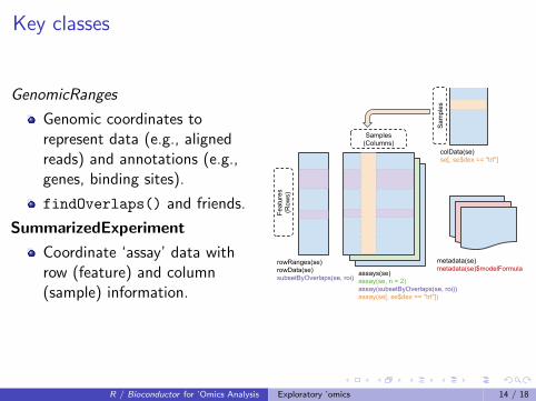
Key classes
GenomicRanges
Genomic coordinates torepresent data (e.g., alignedreads) and annotations (e.g.,genes, binding sites).
findOverlaps() and friends.
SummarizedExperiment
Coordinate ‘assay’ data withrow (feature) and column(sample) information.
> gr = exons(TxDb.Hsapiens.UCSC.hg19.knownGene); grGRanges with 289969 ranges and 1 metadata column: seqnames ranges strand | exon_id <Rle> <IRanges> <Rle> | <integer> [1] chr1 [11874, 12227] + | 1 [2] chr1 [12595, 12721] + | 2 [3] chr1 [12613, 12721] + | 3 ... ... ... ... ... ... [289967] chrY [59358329, 59359508] - | 277748 [289968] chrY [59360007, 59360115] - | 277749 [289969] chrY [59360501, 59360854] - | 277750 --- seqinfo: 93 sequences (1 circular) from hg19 genome
DataFrame mcols(gr) gr$exon_id
GRanges length(gr); gr[1:5] seqnames(gr) start(gr) end(gr) width(gr) strand(gr)
Seqinfo seqlevels(gr) seqlengths(gr) genome(gr)
R / Bioconductor for ’Omics Analysis Exploratory ’omics 14 / 18
Key classes
GenomicRanges
Genomic coordinates torepresent data (e.g., alignedreads) and annotations (e.g.,genes, binding sites).
findOverlaps() and friends.
SummarizedExperiment
Coordinate ‘assay’ data withrow (feature) and column(sample) information.
colData(se)se[, se$dex == "trt"]
rowRanges(se)rowData(se)subsetByOverlaps(se, roi)
assays(se)assay(se, n = 2)assay(subsetByOverlaps(se, roi))assay(se[, se$dex == "trt"])
metadata(se)metadata(se)$modelFormula
Samples (Columns)
Sam
ples
Feat
ures
(R
ows)
R / Bioconductor for ’Omics Analysis Exploratory ’omics 14 / 18

Big data
GenomicFiles
Management of file collections,e.g., VCF, BAM, BED.
BiocParallel
Parallel evaluation on cores,clusters, clouds.
HDF5Array
On-disk storage.
Delayed evaluation.
Incorporates intoSummarizedExperiment.
Key strategies
Efficient R code
Restriction to data of interest
Chunk-wise iteration throughlarge data
R / Bioconductor for ’Omics Analysis Exploratory ’omics 15 / 18

From student to developer
A common transition
Naive users become proficient while developing domain expertise thatthey share with others in their lab or more broadly
Share via packages!
Resources
Learning: course material, videos, workflows, vignettes.
Using: vignettes, help pages, support site.
Developing: Wicham’s R Packages9, Bioconductor developerresources10, bioc-devel mailing list
9http://r-pkgs.had.co.nz/10http://bioconductor.org/developers/
R / Bioconductor for ’Omics Analysis From student to developer 16 / 18

Developer
Really easy!
Use devtools to create() a package
Add functions to the R directory
Add documentation with roxygen2
Add ’markdown’ vignettes using knitr
Best practices
build(), check(), install()
Version control – github
Unit tests, e.g., using testthat
‘Continuous integration’
R / Bioconductor for ’Omics Analysis From student to developer 17 / 18

Acknowledgments
Core team (current & recent): Yubo Cheng, Valerie Obenchain, HervePages, Marcel Ramos, Lori Shepherd, Dan Tenenbaum, Greg Wargula.
Technical advisory board: Vincent Carey, Kasper Hansen, WolfgangHuber, Robert Gentleman, Rafael Irizzary, Levi Waldron, MichaelLawrence, Sean Davis, Aedin Culhane
Scientific advisory board: Simon Tavare (CRUK), Paul Flicek(EMBL/EBI), Simon Urbanek (AT&T), Vincent Carey (Brigham &Women’s), Wolfgang Huber (EBI), Rafael Irizzary (Dana Farber), RobertGentleman (23andMe)
Research reported in this presentation was supported by the NationalHuman Genome Research Institute and the National Cancer Institute ofthe National Institutes of Health under award numbers U41HG004059 andU24CA180996. The content is solely the responsibility of the authors anddoes not necessarily represent the official views of the National Institutesof Health.
R / Bioconductor for ’Omics Analysis Acknowledgments 18 / 18
Top Related