Download - Quanser NI-ELVIS Trainer (QNET) Series: QNET Experiment ...galia.fc.uaslp.mx/~ducd/cursos/control2/QNET-Exp1-Speed_Student.pdf · Quanser NI-ELVIS Trainer (QNET) Series: QNET Experiment

Quanser NI-ELVIS Trainer (QNET) Series:

QNET Experiment #01:DC Motor Speed Control

DC Motor Control Trainer (DCMCT)

Student Manual

DCMCT Speed Control Laboratory Manual

Table of Contents1. Laboratory Objectives.........................................................................................................12. References...........................................................................................................................13. DCMCT Plant Presentation.................................................................................................1

3.1. Component Nomenclature...........................................................................................13.2. DCMCT Plant Description..........................................................................................2

4. Pre-Lab Assignment............................................................................................................24.1. Exercise: Open-loop Modeling...................................................................................3

5. In-Lab Session.....................................................................................................................55.1. System Hardware Configuration..................................................................................55.2. Experimental Procedure...............................................................................................5

Revision: 01 Page: i


1. Laboratory ObjectivesThe objective of this experiment is to design a closed-loop control system that regulates thespeed of the DC motor. The mathematical model of a DC motor is reviewed and its physicalparameters are identified. Once the model is verified, it is used to design a proportional-integral, or PI, controller.

Regarding the Gray Boxes:

The gray boxes present in the instructor manual are not intended for the students asthey provide solutions to the pre-lab assignments and contain typical experimental resultsfrom the laboratory procedure.

2. References[1] NI-ELVIS User Manual[2] DCMCT User Manual

3. DCMCT Plant Presentation

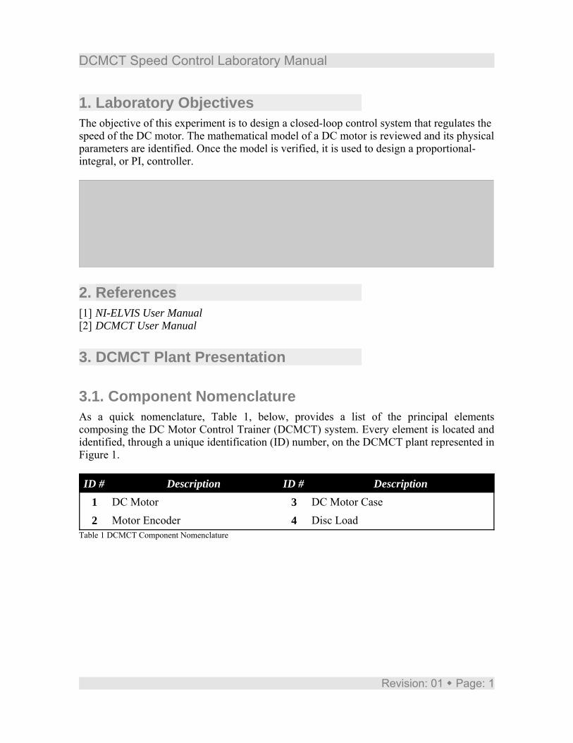
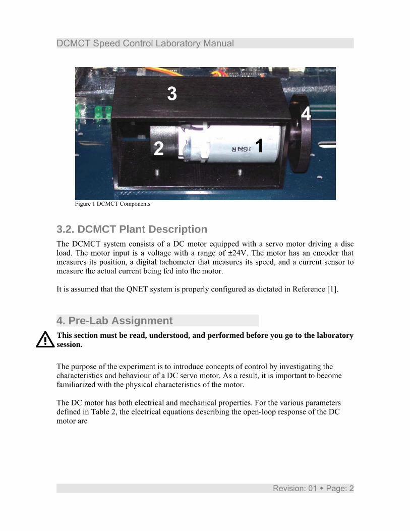
3.1. Component NomenclatureAs a quick nomenclature, Table 1, below, provides a list of the principal elementscomposing the DC Motor Control Trainer (DCMCT) system. Every element is located andidentified, through a unique identification (ID) number, on the DCMCT plant represented inFigure 1.

ID # Description ID # Description1 DC Motor 3 DC Motor Case

2 Motor Encoder 4 Disc LoadTable 1 DCMCT Component Nomenclature

Revision: 01 Page: 1


Figure 1 DCMCT Components

3.2. DCMCT Plant DescriptionThe DCMCT system consists of a DC motor equipped with a servo motor driving a discload. The motor input is a voltage with a range of ±24V. The motor has an encoder thatmeasures its position, a digital tachometer that measures its speed, and a current sensor tomeasure the actual current being fed into the motor.

It is assumed that the QNET system is properly configured as dictated in Reference [1].

4. Pre-Lab AssignmentThis section must be read, understood, and performed before you go to the laboratorysession.

The purpose of the experiment is to introduce concepts of control by investigating thecharacteristics and behaviour of a DC servo motor. As a result, it is important to becomefamiliarized with the physical characteristics of the motor.

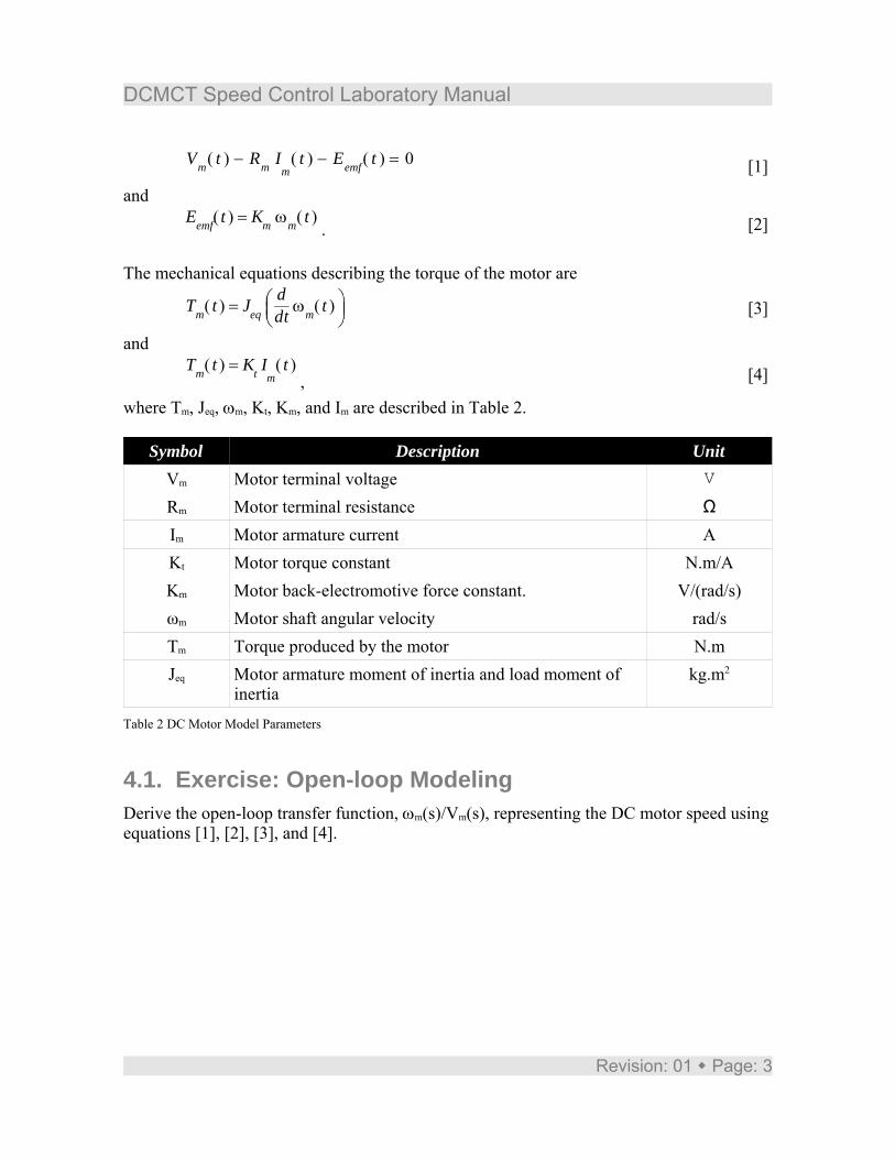
The DC motor has both electrical and mechanical properties. For the various parametersdefined in Table 2, the electrical equations describing the open-loop response of the DCmotor are



= − − ( )Vm t Rm ( )Im

t ( )Eemf t 0 [1]

and = ( )Eemf t Km ( )ωm t

. [2]

The mechanical equations describing the torque of the motor are

= ( )Tm t Jeq⎛⎝⎜⎜

⎞⎠⎟⎟d

dt ( )ωm t [3]

and = ( )Tm t Kt ( )I

mt

, [4]

where Tm, Jeq, ωm, Kt, Km, and Im are described in Table 2.

Symbol Description UnitVm Motor terminal voltage V

Rm Motor terminal resistance ΩIm Motor armature current AKt Motor torque constant N.m/AKm Motor back-electromotive force constant. V/(rad/s)ωm Motor shaft angular velocity rad/sTm Torque produced by the motor N.mJeq Motor armature moment of inertia and load moment of

inertiakg.m2

Table 2 DC Motor Model Parameters

4.1. Exercise: Open-loop ModelingDerive the open-loop transfer function, ωm(s)/Vm(s), representing the DC motor speed usingequations [1], [2], [3], and [4].



Solution:Combine the mechanical equations by substituting the Laplace transform of equation [4]into the Laplace of [3] and solve for current Im(s)

.

Substituting the above equation and the Laplace of [2] into the Laplace transform of [1]gives

.

The open-loop transfer function of the DC motor is found by solving for ωm(s)/Vm(s):

.



5. In-Lab Session

5.1. System Hardware ConfigurationThis in-lab session is performed using the NI-ELVIS system equipped with a QNET-DCMCT board and the Quanser Virtual Instrument (VI) controller fileQNET_DCMCT_Lab_01_Speed_Control.vi. Please refer to Reference [2] for the setup andwiring information required to carry out the present control laboratory. Reference [2] alsoprovides the specifications and a description of the main components composing yoursystem.

Before beginning the lab session, ensure the system is configured as follows: QNET DC Motor Control Trainer module is connected to the ELVIS. ELVIS Communication Switch is set to BYPASS. DC power supply is connected to the QNET DC Motor Control Trainer module. The 4 LEDs +B, +15V, -15V, +5V on the QNET module should be ON.

5.2. Experimental Procedure

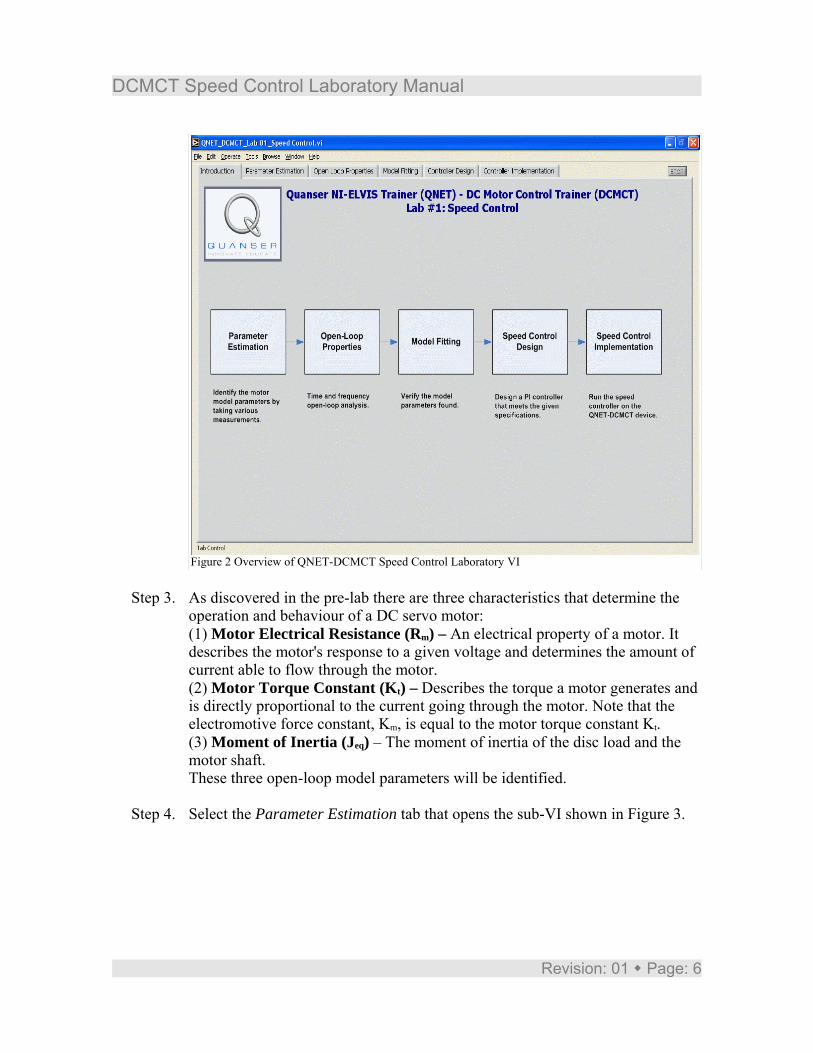
The sections below correspond to the tabs in the VI, shown in Figure 2. Please follow thesteps described below:

Step 1. Read through Section 5.1 and go through the setup guide in Reference [2]Step 2. Run the VI controller QNET_DCMCT_Lab_01_Speed_Control.vi shown in

Figure 2. The speed control VI shown in Figure 2 is the top-level VI that willguide you throughout the laboratory.



Figure 2 Overview of QNET-DCMCT Speed Control Laboratory VI

Step 3. As discovered in the pre-lab there are three characteristics that determine theoperation and behaviour of a DC servo motor:(1) Motor Electrical Resistance (Rm) – An electrical property of a motor. Itdescribes the motor's response to a given voltage and determines the amount ofcurrent able to flow through the motor.(2) Motor Torque Constant (Kt) – Describes the torque a motor generates andis directly proportional to the current going through the motor. Note that theelectromotive force constant, Km, is equal to the motor torque constant Kt.(3) Moment of Inertia (Jeq) – The moment of inertia of the disc load and themotor shaft.These three open-loop model parameters will be identified.

Step 4. Select the Parameter Estimation tab that opens the sub-VI shown in Figure 3.



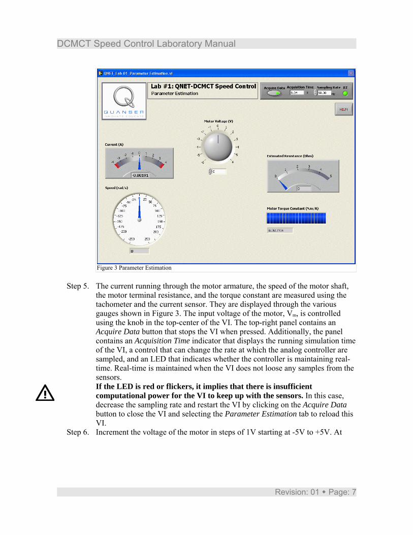
Figure 3 Parameter Estimation

Step 5. The current running through the motor armature, the speed of the motor shaft,the motor terminal resistance, and the torque constant are measured using thetachometer and the current sensor. They are displayed through the variousgauges shown in Figure 3. The input voltage of the motor, Vm, is controlledusing the knob in the top-center of the VI. The top-right panel contains anAcquire Data button that stops the VI when pressed. Additionally, the panelcontains an Acquisition Time indicator that displays the running simulation timeof the VI, a control that can change the rate at which the analog controller aresampled, and an LED that indicates whether the controller is maintaining real-time. Real-time is maintained when the VI does not loose any samples from thesensors.If the LED is red or flickers, it implies that there is insufficientcomputational power for the VI to keep up with the sensors. In this case,decrease the sampling rate and restart the VI by clicking on the Acquire Databutton to close the VI and selecting the Parameter Estimation tab to reload thisVI.

Step 6. Increment the voltage of the motor in steps of 1V starting at -5V to +5V. At



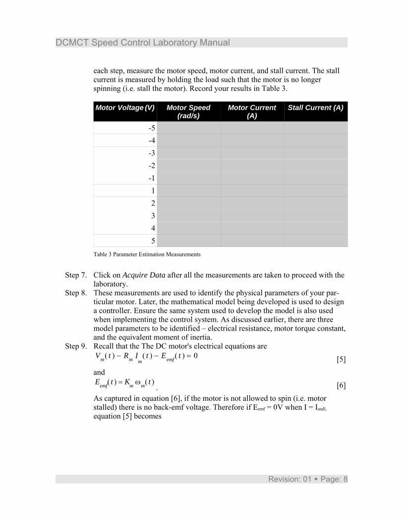
each step, measure the motor speed, motor current, and stall current. The stallcurrent is measured by holding the load such that the motor is no longerspinning (i.e. stall the motor). Record your results in Table 3.

Motor Voltage (V) Motor Speed(rad/s)

Motor Current(A)

Stall Current (A)

-5 -171 -0.189 -1.70-4 -130 -0.180 -1.27-3 -89 -0.172 -0.90-2 -48 -0.169 -0.63-1 -7 -0.180 -0.261 6 0.298 0.272 50 0.217 0.763 91 0.212 1.054 133 0.212 1.435 175 0.217 4.79

Table 3 Parameter Estimation Measurements

Step 7. Click on Acquire Data after all the measurements are taken to proceed with thelaboratory.

Step 8. These measurements are used to identify the physical parameters of your par-ticular motor. Later, the mathematical model being developed is used to designa controller. Ensure the same system used to develop the model is also usedwhen implementing the control system. As discussed earlier, there are threemodel parameters to be identified – electrical resistance, motor torque constant,and the equivalent moment of inertia.

Step 9. Recall that the The DC motor's electrical equations are = − − ( )Vm t Rm ( )I

mt ( )Eemf t 0 [5]

and = ( )Eemf t Km ( )ωm t

. [6]

As captured in equation [6], if the motor is not allowed to spin (i.e. motorstalled) there is no back-emf voltage. Therefore if Eemf = 0V when I = Istall,

equation [5] becomes



= Rm

( )Vm t( )I

stallt

.[7]

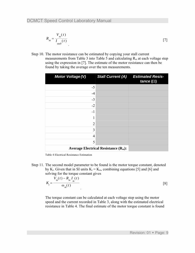
Step 10. The motor resistance can be estimated by copying your stall currentmeasurements from Table 3 into Table 5 and calculating Rm at each voltage stepusing the expression in [7]. The estimate of the motor resistance can then befound by taking the average over the ten measurements.

Motor Voltage (V) Stall Current (A) Estimated Resis-tance (Ω)

-5 -1.70 2.90-4 -1.27 3.15-3 -0.90 3.33-2 -0.63 3.17-1 -0.26 3.851 0.27 3.732 0.76 2.643 1.05 2.864 1.43 2.805 4.79 2.79

Average Electrical Resistance (Rm): 3.12Table 4 Electrical Resistance Estimation

Step 11. The second model parameter to be found is the motor torque constant, denotedby Kt. Given that in SI units Kt = Km, combining equations [5] and [6] andsolving for the torque constant gives

= Kt

− ( )Vm t Rm ( )Im

t

( )ωm t.

[8]

The torque constant can be calculated at each voltage step using the motorspeed and the current recorded in Table 3, along with the estimated electricalresistance in Table 4. The final estimate of the motor torque constant is found



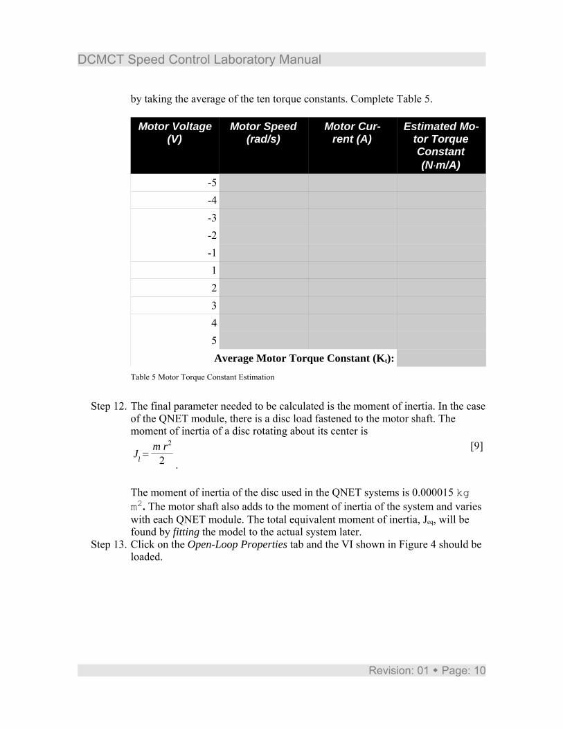
by taking the average of the ten torque constants. Complete Table 5.

Motor Voltage(V)

Motor Speed(rad/s)

Motor Cur-rent (A)

Estimated Mo-tor TorqueConstant(N⋅m/A)

-5 -171 -0.189 0.0258-4 -130 -0.180 0.0264-3 -89 -0.172 0.0277-2 -48 -0.169 0.0307-1 -7 -0.180 0.06261 7 0.298 0.01002 50 0.217 0.02653 91 0.212 0.02574 133 0.212 0.02515 175 0.217 0.0247Average Motor Torque Constant (Kt): 0.0285

Table 5 Motor Torque Constant Estimation

Step 12. The final parameter needed to be calculated is the moment of inertia. In the caseof the QNET module, there is a disc load fastened to the motor shaft. Themoment of inertia of a disc rotating about its center is

= Jlm r2

2 .

[9]

The moment of inertia of the disc used in the QNET systems is 0.000015 kgm2. The motor shaft also adds to the moment of inertia of the system and varieswith each QNET module. The total equivalent moment of inertia, Jeq, will befound by fitting the model to the actual system later.

Step 13. Click on the Open-Loop Properties tab and the VI shown in Figure 4 should beloaded.



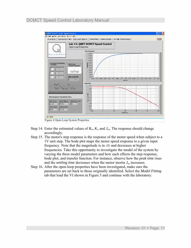
Figure 4 Open-Loop System Properties

Step 14. Enter the estimated values of Rm, Kt, and Jeq. The response should changeaccordingly.

Step 15. The motor's step response is the response of the motor speed when subject to a1V unit step. The bode plot maps the motor speed response to a given inputfrequency. Note that the magnitude is in dB and decreases at higherfrequencies. Take this opportunity to investigate the model of the system byvarying the three model parameters and how each effects the step response,bode plot, and transfer function. For instance, observe how the peak time risesand the settling time decreases when the motor inertia Jeq increases.

Step 16. After the open-loop properties have been investigated, make sure theparameters are set back to those originally identified. Select the Model Fittingtab that load the VI shown in Figure 5 and continue with the laboratory.



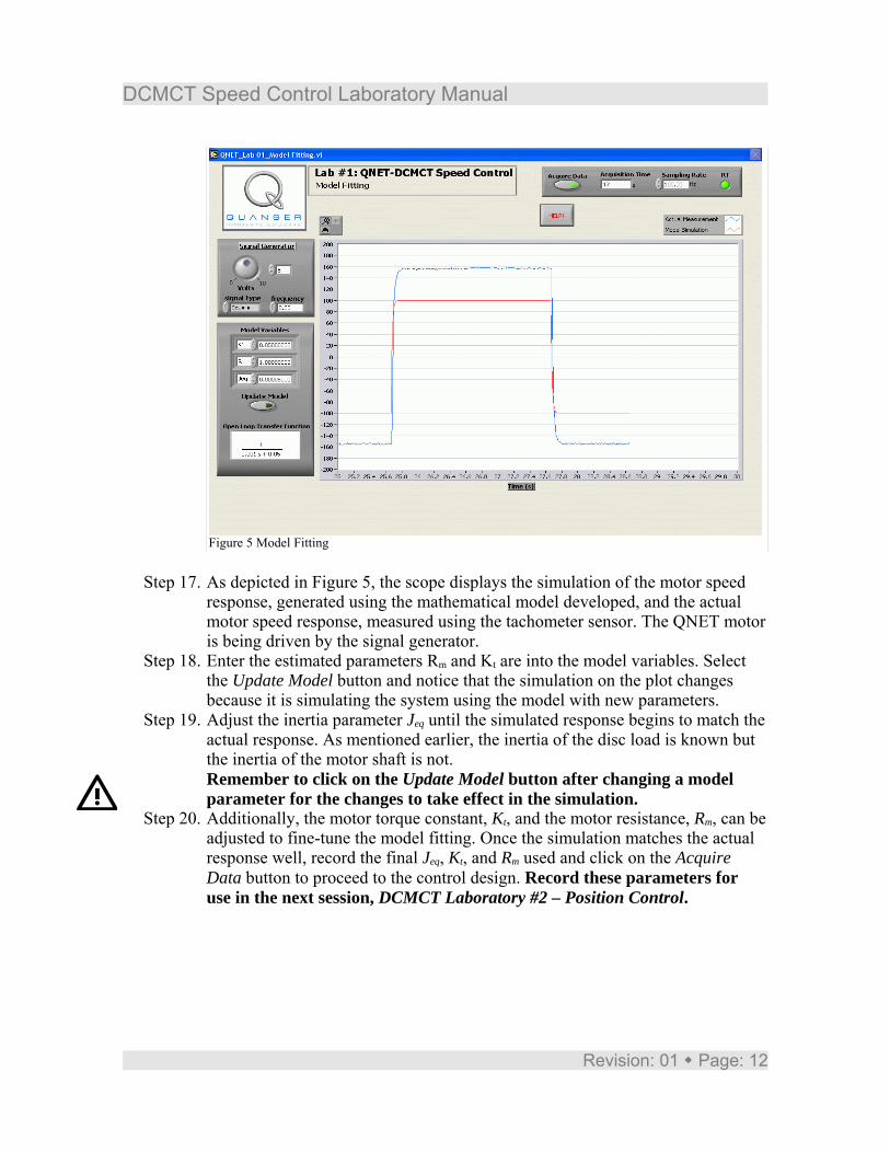
Figure 5 Model Fitting

Step 17. As depicted in Figure 5, the scope displays the simulation of the motor speedresponse, generated using the mathematical model developed, and the actualmotor speed response, measured using the tachometer sensor. The QNET motoris being driven by the signal generator.

Step 18. Enter the estimated parameters Rm and Kt are into the model variables. Selectthe Update Model button and notice that the simulation on the plot changesbecause it is simulating the system using the model with new parameters.

Step 19. Adjust the inertia parameter Jeq until the simulated response begins to match theactual response. As mentioned earlier, the inertia of the disc load is known butthe inertia of the motor shaft is not.Remember to click on the Update Model button after changing a modelparameter for the changes to take effect in the simulation.

Step 20. Additionally, the motor torque constant, Kt, and the motor resistance, Rm, can beadjusted to fine-tune the model fitting. Once the simulation matches the actualresponse well, record the final Jeq, Kt, and Rm used and click on the AcquireData button to proceed to the control design. Record these parameters foruse in the next session, DCMCT Laboratory #2 – Position Control.



Model Fitted Parameter MeasuredValue

Unit

Rm 3.12 Ω

Kt 0.0295 N⋅m/AJeq 1.93E-005 kg⋅m2

Table 6 Model Fitted Parameters

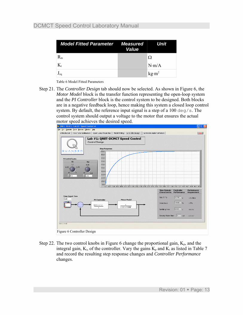
Step 21. The Controller Design tab should now be selected. As shown in Figure 6, theMotor Model block is the transfer function representing the open-loop systemand the PI Controller block is the control system to be designed. Both blocksare in a negative feedback loop, hence making this system a closed loop controlsystem. By default, the reference input signal is a step of a 100 deg/s. Thecontrol system should output a voltage to the motor that ensures the actualmotor speed achieves the desired speed.

Figure 6 Controller Design

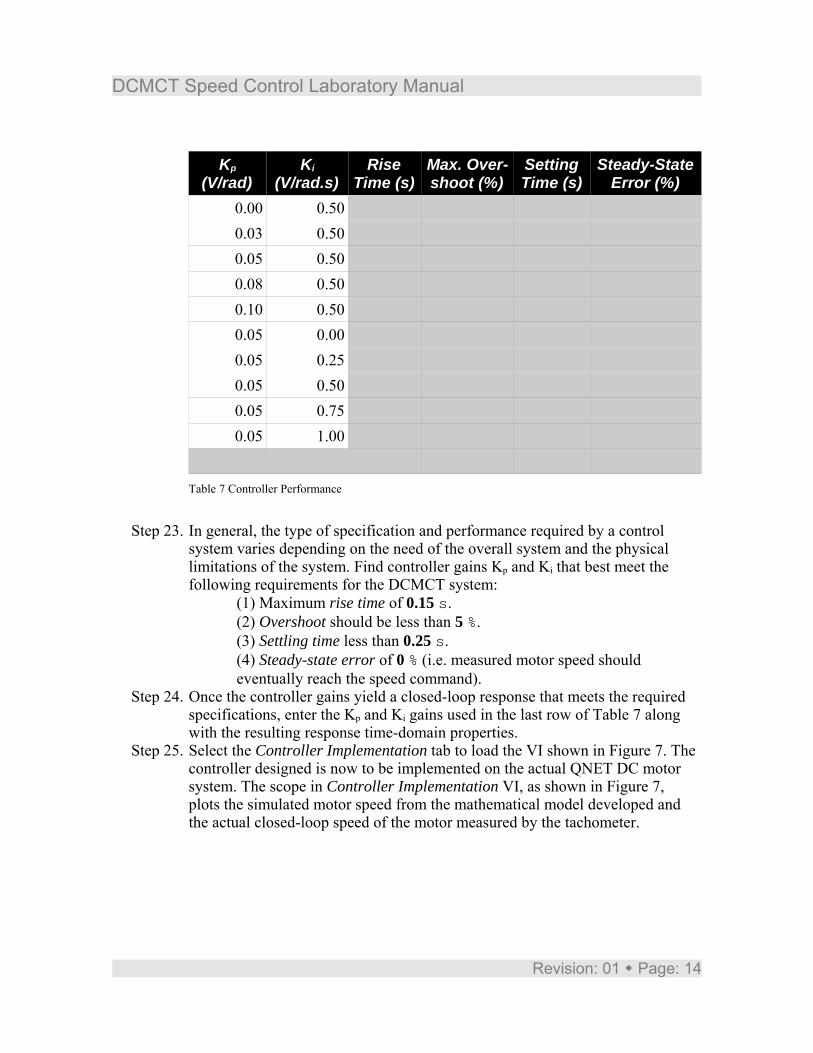
Step 22. The two control knobs in Figure 6 change the proportional gain, Kp, and theintegral gain, Ki, of the controller. Vary the gains Kp and Ki as listed in Table 7and record the resulting step response changes and Controller Performancechanges.



Kp

(V/rad)Ki

(V/rad.s)Rise

Time (s)Max. Over-shoot (%)

SettingTime (s)

Steady-StateError (%)

0.00 0.50 0.103 22.300 0.719 0.00.03 0.50 0.120 1.050 0.299 0.00.05 0.50 0.131 -0.008 0.384 0.00.08 0.50 0.135 -0.007 0.581 0.00.10 0.50 0.132 -0.006 0.683 0.00.05 0.00 0.001 -0.270 0.128 36.30.05 0.25 0.334 -0.011 0.990 0.00.05 0.50 0.131 -0.008 0.384 0.00.05 0.75 0.078 0.724 0.145 0.00.05 1.00 0.067 3.980 0.257 0.00.55 0.04 0.137 0.274 0.244 0.0

Table 7 Controller Performance

Step 23. In general, the type of specification and performance required by a controlsystem varies depending on the need of the overall system and the physicallimitations of the system. Find controller gains Kp and Ki that best meet thefollowing requirements for the DCMCT system:

(1) Maximum rise time of 0.15 s.(2) Overshoot should be less than 5 %.(3) Settling time less than 0.25 s.(4) Steady-state error of 0 % (i.e. measured motor speed shouldeventually reach the speed command).

Step 24. Once the controller gains yield a closed-loop response that meets the requiredspecifications, enter the Kp and Ki gains used in the last row of Table 7 alongwith the resulting response time-domain properties.

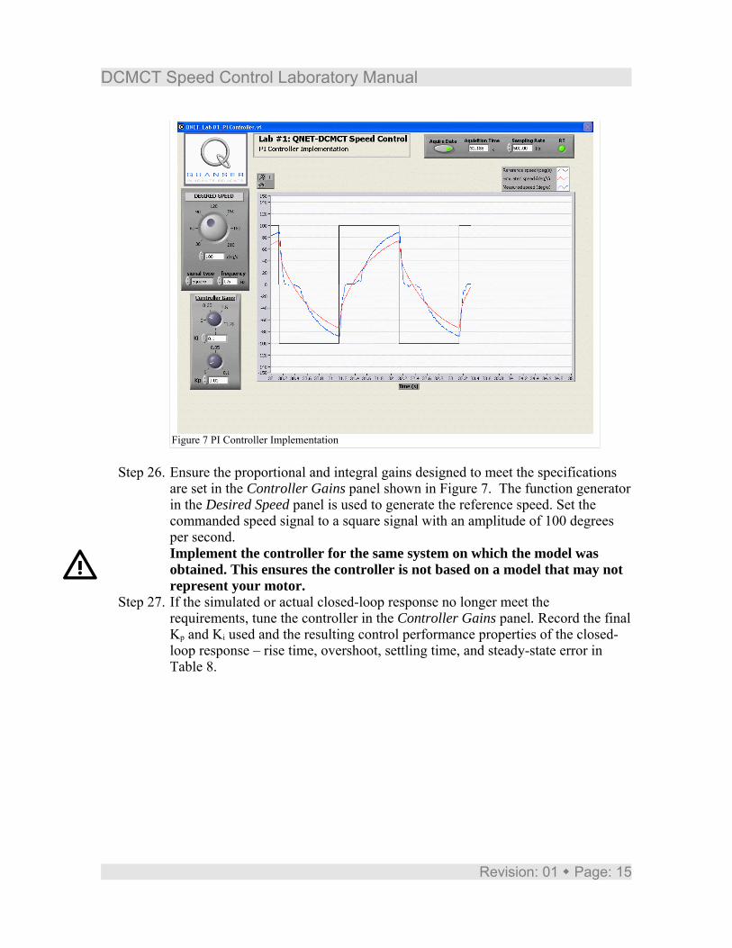
Step 25. Select the Controller Implementation tab to load the VI shown in Figure 7. Thecontroller designed is now to be implemented on the actual QNET DC motorsystem. The scope in Controller Implementation VI, as shown in Figure 7,plots the simulated motor speed from the mathematical model developed andthe actual closed-loop speed of the motor measured by the tachometer.



Figure 7 PI Controller Implementation

Step 26. Ensure the proportional and integral gains designed to meet the specificationsare set in the Controller Gains panel shown in Figure 7. The function generatorin the Desired Speed panel is used to generate the reference speed. Set thecommanded speed signal to a square signal with an amplitude of 100 degreesper second.Implement the controller for the same system on which the model wasobtained. This ensures the controller is not based on a model that may notrepresent your motor.

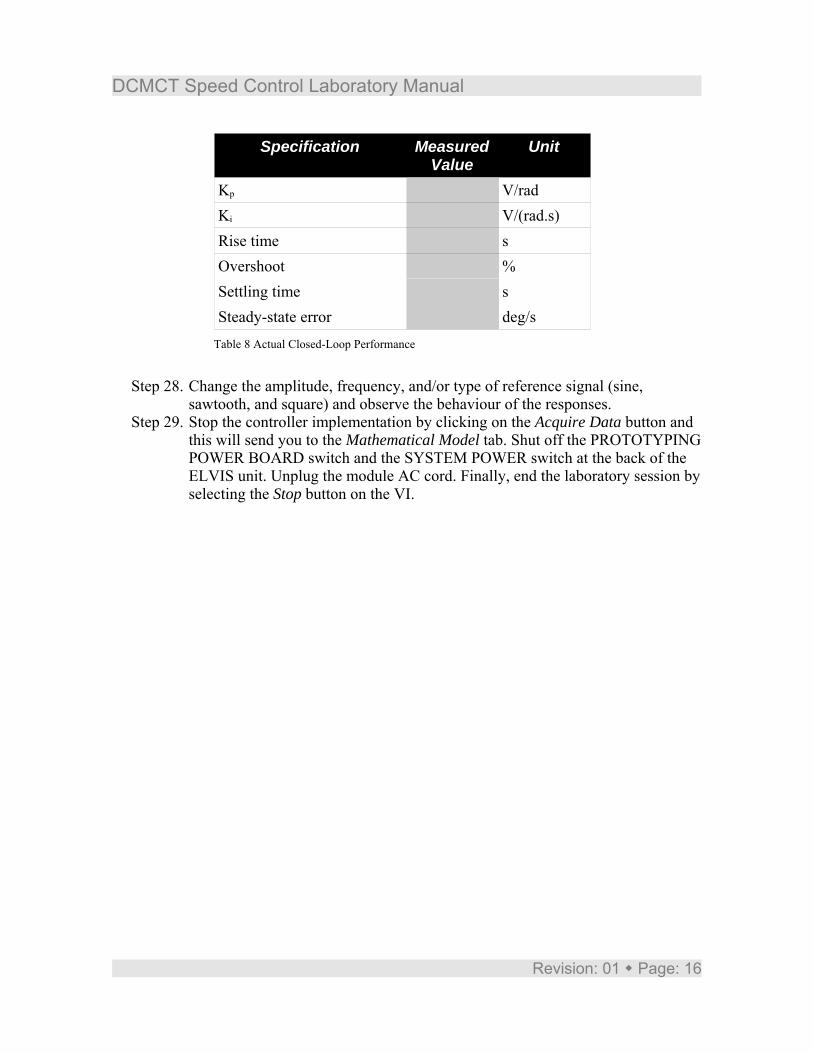
Step 27. If the simulated or actual closed-loop response no longer meet therequirements, tune the controller in the Controller Gains panel. Record the finalKp and Ki used and the resulting control performance properties of the closed-loop response – rise time, overshoot, settling time, and steady-state error inTable 8.



Specification MeasuredValue

Unit

Kp 0.04 V/radKi 0.65 V/(rad.s)Rise time 0.12 sOvershoot 0.0 %Settling time 0.24 sSteady-state error 0.0 deg/s

Table 8 Actual Closed-Loop Performance

Step 28. Change the amplitude, frequency, and/or type of reference signal (sine,sawtooth, and square) and observe the behaviour of the responses.

Step 29. Stop the controller implementation by clicking on the Acquire Data button andthis will send you to the Mathematical Model tab. Shut off the PROTOTYPINGPOWER BOARD switch and the SYSTEM POWER switch at the back of theELVIS unit. Unplug the module AC cord. Finally, end the laboratory session byselecting the Stop button on the VI.
