


Languages
Pages
Legal


Qualification of innovative floating substructures for
10MW wind turbines and water depths greater than 50m
Project acronym LIFES50+ Grant agreement 640741
Collaborative project Start date 2015-06-01 Duration 40 months
Deliverable D4.1 Simple numerical models for upscaled design
Lead Beneficiary USTUTT
Due date 2016-02-29
Delivery date 2016-04-01
Dissemination level Public
Status Final
Classification Unrestricted
Keywords Floating wind modelling, loads analysis, simplified, optimization
Company document number Click here to enter text.
The research leading to these results has received funding from the
European Union Horizon2020 programme under the agreement
H2020-LCE-2014-1-640741.

D4.1 Simple numerical models for upscaled design
LIFES50+ Deliverable, project 640741 2/45
Disclaimer
The content of the publication herein is the sole responsibility of the publishers and it does not neces-sarily represent the views expressed by the European Commission or its services.
While the information contained in the documents is believed to be accurate, the authors(s) or any other participant in the LIFES50+ consortium make no warranty of any kind with regard to this material including, but not limited to the implied warranties of merchantability and fitness for a particular pur-pose.
Neither the LIFES50+ Consortium nor any of its members, their officers, employees or agents shall be responsible or liable in negligence or otherwise howsoever in respect of any inaccuracy or omission herein.
Without derogating from the generality of the foregoing neither the LIFES50+ Consortium nor any of its members, their officers, employees or agents shall be liable for any direct or indirect or consequential loss or damage caused by or arising from any information advice or inaccuracy or omission herein.
Document information
Version Date Description
1 2016-03-01 Draft
Prepared by Lemmer, F.; Müller, K.; Pegalajar-Jurado, A; Borg, M.;
Bredmose, H.;
Reviewed
by
Aguirre, G., Landbø, T., Andersen, H.S.
Approved
by
Enter names
2 2016-03-29 Final version for QA before submission to EU
Prepared by Lemmer, F.; Müller, K.; Pegalajar-Jurado, A; Borg, M.;
Bredmose, H.;
Reviewed by Petter Andreas Berthelsen
Approved by Jan Arthur Norbeck
3 2015-04-21 Public version
Prepared by Lemmer, F.; Müller, K.; Pegalajar-Jurado, A; Borg, M.;
Bredmose, H.;
Reviewed by Enter names
Approved by Enter names
In order to enter a new version row, copy the above and paste into left most cell.
Authors Organization
Lemmer, F. USTUTT
Müller, K. USTUTT
Pegalajar-Jurado, A. DTU
Borg, M. DTU
Bredmose, H. DTU
Contributors Organization

D4.1 Simple numerical models for upscaled design
LIFES50+ Deliverable, project 640741 3/45
Definitions & Abbreviations
1p One time per rotor revolution
3p Three times per rotor revolution
AQWA Potential flow simulation model by Ansys
BEM Blade Element Momentum
Bladed Aero-hydro-servo-elastic simulation model by DNV-GL
CPU Central Processing Unit
DEL Damage-Equivalent Load
DLC Design Load Case
DOF Degree Of Freedom
EOG Extreme Operational Gust
EQM Equation of motion
FAST Aero-hydro-servo-elastic simulation model by NREL
FEM Finite Element Model
FFT Fast Fourier Transform
FOWT Floating Offshore Wind Turbine
HAWC2 Aero-hydro-servo-elastic simulation model by DTU
MIMO Multiple-input-multiple-output
MSL Mean Sea Level
NMPC Nonlinear model-predictive control
OC3 Offshore Code Comparison Collaboration
OC4 Offshore Code Comparison Collaboration Continuation
OC5 Offshore Code Comparison Collaboration Continuation with Correlation
ODE Ordinary Differential Equation
PI Proportional-Integral (controller)
PSD Power spectral density
QuLA Quick Load Analysis (simplified model by DTU)
RAO Response Amplitude Operator
RNA Rotor-nacelle assembly
RWT Reference Wind Turbine
SIMA Floating systems simulation model by Marintek
SISO Single-input-single-output
SLOW Simplified Low-Order Wind turbine (simplified model by USTUTT)
SoA State-of-the-Art
SWL Sea Water Level
TSR Tip-Speed Ratio
WAMIT Wave analysis simulation model by MIT
WP Work Package
Symbols
Added mass matrix
Heave plate cross-sectional area
Radiation damping matrix
Model input (SLOW)
Aerodynamic damping coefficient
Hydrostatic restoring
Linearized mooring system stiffness
Drag coefficient
, Aerodynamic power and thrust coefficients
Effective platform diameter (for drag force calculation)
Tower bending stiffness
External force vector
D4.1 Simple numerical models for upscaled design
LIFES50+ Deliverable, project 640741 4/45
Aerodynamic force
Hydrodynamic wave excitation force
Hydrodynamic drag force
Hydrodynamic force
Frequency
, Horizontal and vertical fairleads forces
Significant wave height
Imaginary unit
Radiation impulse response kernel
Applied forces
Proportional gain (controller)
Structural mass matrix
Tower-base bending moment
RNA & platform mass, respectively (QuLA)
Tower mass
Linearized velocity-dependent forces
Coriolis, centrifugal and gyroscopic forces
Generalized coordinates
Linearized position-dependent forces
Rotor radius
Horizontal hub velocity
Time constant (controller)
Peak spectral period
Time
Differential model input
State vector
Platform surge displacement
Tower-top fore-aft displacement
Rotor-effective wind speed/Mean wind speed
Relative rotor-effective wind speed
, Horizontal and vertical fluid particle velocity
, Horizontal and vertical platform velocity
, Horizontal and vertical fairlead displacement
Horizontal hub displacement
Platform heave displacement
Platform pitch displacement
Wave elevation
Blade pitch angle
Tip-speed ratio (TSR)
Generalized rigid-body coordinates of floating body
Density
Angular frequency
Rotor speed
Reference (rated) rotor speed

D4.1 Simple numerical models for upscaled design
LIFES50+ Deliverable, project 640741 5/45
Executive Summary
This deliverable presents parametric design models for an upscaling of the LIFES50+ platforms as
well as simplified coupled models. The frequency-domain model QuLA by DTU and the time-domain
multibody model SLOW by USTUTT are introduced. The two models feature high computational
efficiency, which is beneficial for early conceptual design calculations. Many different load cases can
be calculated with QuLA, featuring a real-time factor of more than 1000. This is due to the nature of
the frequency-domain description - but even SLOW, written in time-domain, simulates about 160
times faster than real time allowing the designer to run many system simulations and sensitivity
studies for early-stage optimization.
Whereas QuLA represents the wind turbine through pre-computed rotor loads and an aerodynamic
damping coefficient SLOW uses an actuator-disk-like approach and therefore includes also the blade-
pitch angle and thus the effects of the control. QuLA’s time-series of the aerodynamic thrust forces
can be obtained from state-of-the-art models, run independently of the simplified models. This has the
advantage that the detailed simulation model is not necessary for the platform designer, avoiding
confidentiality issues. SLOW consists of a nonlinear multibody system, which can be easily adjusted
for a new model layout. It uses symbolic programming for easy portability and high computational
speed. Various levels of fidelity, like a linearized version besides the nonlinear one allow a
comparison of different levels of modeling detail.
The models are compared to simulations of the state-of-the-art tool FAST in a comprehensive study of
system identification, fatigue and extreme load cases of the LIFES50+ design basis. One-hour
simulations for the whole operating range with three different wave environments are performed and
additionally, with the 50-year extreme wave climate. Prior to this, system identification tests are run,
checking the transient and steady-state behavior. For this study, a generic concrete semi-submersible
platform is used together with the DTU10MW reference wind turbine. A conceptual controller
accounting for the floating foundation has been developed for the present deliverable in order to
simulate the whole operating range. It includes a common nonlinear state feedback below rated
conditions and for above rated-wind speeds, which are critical for floating wind turbines, a
proportional-integral controller with gain scheduling. This ensures constant system dynamics of the
floating wind turbine throughtout the operating range.
In general, a good agreement can be seen between the simplified models and the reference model in
terms of eigenfrequencies, steady states and wave response, proving their consistency. The fatigue
loads in operational conditions agree fairly well and can therefore be used for conceptual design
calculations. For extreme loads, however, notable deviations occur. One reason for this is the strong
nonlinearity of the external aerodynamic and hydrodynamic forces. In the 50-year extreme sea states
the rotor experiences extreme inflow conditions, which challenge the simplified models. Here, an
application of the simplified models needs to be carefully evaluated. The detailed differences are
summarized in a discussion of the model features, their tuning and their applicability across the range
of design load cases. The last aspect will be worked on in later deliverables of WP4 in LIFES50+.

D4.1 Simple numerical models for upscaled design
LIFES50+ Deliverable, project 640741 6/45
Contents
Introduction ............................................................................................................................................. 7
Modelling Approaches .................................................................................................................... 7 1
1.1 Parametric spreadsheet calculations ........................................................................................ 8
1.2 Parametric panel code calculations ....................................................................................... 10
1.3 Simplified aero-hydro-servo-elastic codes ............................................................................ 11
Reference turbine and floating platform ........................................................................................ 18 2
2.1 Platform ................................................................................................................................. 19
2.2 Mooring system ..................................................................................................................... 21
2.3 Wind turbine .......................................................................................................................... 23
2.4 Controller............................................................................................................................... 23
Selection of Load Cases ................................................................................................................ 25 3
3.1 System identification ............................................................................................................. 25
3.2 Design load cases .................................................................................................................. 26
Results ........................................................................................................................................... 27 4
4.1 System identification ............................................................................................................. 28
4.2 Design load cases .................................................................................................................. 31
Conclusions ................................................................................................................................... 40 5
Bibliography .................................................................................................................................. 43 6
Checklist for Deliverables ............................................................................................................. 45 7
7.1 Time table .............................................................................................................................. 45
7.2 Quality assurance checklist ................................................................................................... 45

D4.1 Simple numerical models for upscaled design
LIFES50+ Deliverable, project 640741 7/45
Introduction Work Package 4 of LIFES50+ examines and develops numerical models of Floating Offshore Wind
Turbines (FOWT) in order to first assess accuracy and subsequently improve state-of-the-art methods
of the numerical FOWT design practice that has been described in the LIFES50+ deliverables D4.4
and D7.4, see [1] and [2]. The work of the partners in this work package addresses a number of aspects
of the numerical design process of floating wind turbines. The results of the specific studies of WP4
will be eventually fed back into general guidelines. This also includes improving simplified design
tools, which is the focus of the present report.
The role of simplified numerical models falls within the conceptual design stage of the floating sup-
port structure design process, where computational efficiency is paramount to evaluating different
configurations in numerous environmental conditions whilst maintaining sufficient accuracy. Numeri-
cal models for offshore wind turbines are often divided into decoupled and coupled models, referring
to the way the combined loads from the rotor and floater are calculated. In the present report, decou-
pled conceptual methods using spreadsheet calculations and parametric panel code simulations by the
University of Stuttgart are addressed first in Section 1.1 and 1.2. Simplified coupled models are then
introduced in Section 1.3. These tools have their origin at the two research partners Technical Univer-
sity of Denmark (DTU) and the University of Stuttgart (USTUTT) and are based on different physical
assumptions leading to a different range of applicability.
The models are applied to the generic DTU 10MW offshore reference wind turbine [3] on the generic
concrete TripleSpar concept developed in the project INNWIND.EU, see [4]. This concept is used in
WP4 until the two LIFES50+ concepts are selected. The load cases considered here have been selected
from the LIFES50+ design basis [5] for site C, West of Barra, which presents the most extreme weath-
er conditions in LIFES50+. Through the evaluation of the results from these load cases, the range of
applicability and limitations of the simplified design tools herein is identified.
The definition of assumptions with decreasing uncertainty throughout the design process and the con-
cept of increasing the level of fidelity continuously during the design of FOWT is the subject of Chap-
ter 1. In Chapter 2 the reference FOWT considered is introduced. The selection of load cases of this
deliverable is topic of Chapter 3 before the results are presented and analysed in Chapter 4. Finally,
Chapter 6 provides some key conclusions from the analyses.
Modelling Approaches 1Modelling tools for FOWT have been improved significantly during the last years. Due to the transient
and nonlinear loading from wind and waves, time-domain simulations are usually performed, as op-
posed to the commonly used frequency-domain methods from the oil and gas industry. There are a
number of open-source and commercial software available, which couple aerodynamic models with
structural multi-body codes, quasi-static or dynamic mooring line models and time-domain hydrody-
namic models. These models normally use Blade Element Momentum (BEM) theory for aerodynam-
ics, modally reduced bodies for the structural multi-body model and the Cummins equation for the
hydrodynamics. These models will be called “state-of-the-art” (SoA) tools in this report
The numerical design process does usually not start with these tools as they require a quite detailed
description of the overall system. At an early design stage, for upscaling and optimization, simpler
models which give a qualitative overview of the feasibility of a concept with low computational cost
are suitable. Here, parametric models for spreadsheet design methods and panel code calculations are

D4.1 Simple numerical models for upscaled design
LIFES50+ Deliverable, project 640741 8/45
presented in Section 1.1 and 1.2. After this, the simplified coupled models are introduced in Section
1.3 – the frequency-domain tool QuLA by DTU in and the simplified coupled model SLOW by
USTUTT.
The different design stages of a floating wind turbine system and its components warrant the use of
different levels of modelling detail and accuracy in numerical design tools. As observed in responses
from questionnaires to concept developers of LIFES50+ in [6], [1], [2] as well as in literature, the sim-
plified numerical models considered in this report provide main results in the first “conceptual design
stage”, see [2] . Higher fidelity state-of-the-art tools, e.g. FAST, Bladed, SIMA, HAWC2, are then
utilized once the whole design space has been explored and a conceptual design has been achieved.
The type and variety of simulated load cases changes as a function of design stage and numerical tools
being used. In LIFES50+, one objective is to develop the concept of interconnected design phases,
load cases and simulation models. This will provide end users a systematic framework whereby types
of simulation models and load cases to consider as a function of design phase are clearly defined. In
this report, model verification procedures and load cases to be considered in conjunction with the
above described simplified numerical tools are studied.
Figure 1 - Numerical design process for FOWT, [6].
The numerical design of floating foundations commonly starts with spreadsheet calculations for the
assessment of the hydrostatic properties and addresses response amplitude operators (RAO). These
two steps as the initial procedures of the numerical FOWT design process are subject to the next two
sections.
1.1 Parametric spreadsheet calculations In this early design phase the material cost can already be assessed giving a good overview of the fea-
sibility of a selected concept. If these models are set up in a parametric way, sensitivities and distinct
properties can be identified early in the design process. Examples are the draft, the material cost relat-
ed to the hydrostatic and dynamic behaviour. In this section such simple parametric models are illus-
trated for the TripleSpar foundation, which is used as a generic concept in this deliverable. It is intro-
duced in Section 2.1.

D4.1 Simple numerical models for upscaled design
LIFES50+ Deliverable, project 640741 9/45
For the concept studies the main constraints with respect to system behaviour (and thus apart from
constraints that are imposed on the design by other stages or parts of the project, e.g. fabrication and
installation, which is considered to be addressed prior to the concept study) are related to the hydro-
static properties: (1) In vertical direction the buoyancy needs to equal the overall mass, (2) in pitch
direction a maximum heeling angle (e.g. between 3 and 7 degrees) is set as a constraint such that all
considered designs ensure this heeling angle at rated thrust. See Table 1 for all constraints and varia-
bles considered in the presented work.
Fixed parameters
(constraints)
Free variables Dependent
variables
Optimization
variables
Sp
rea
dsh
eet
Buoyancy to
support system
Constant heel-
ing angle under
rated wind
loads.
Column diameter
Column spacing
Draft
Tripod wall
thickness &
diameter
Material cost
Draft (depending
on site + port)
Para
met
ric
pa
n-
el c
od
e
RAO peak pe-
riod
Low wave load
amplification at
wave frequencies
Table 1 - Constraints and optimization variables.
Figure 2 shows the material cost and the draft for different column spacings on the horizontal axis and
column radii on the vertical axis. The draft results from the constraints are also included. The draft
might be selected based on the site but it might also be defined as an optimization variable in order to
target a foundation with low draft, flexible to multiple sites. The assumptions of these calculations are
a constant wall thickness of the columns with reinforced concrete. The required steel mass of the tri-
pod has been approximated through static FEM calculations for two designs with linear interpolations
for column spacings inbetween.
Although many design steps are omitted here, this example puts the next part on the de-coupled poten-
tial flow calculations in order to the subsequent simplified coupled methods.

D4.1 Simple numerical models for upscaled design
LIFES50+ Deliverable, project 640741 10/45
Figure 2 – Spreadsheet studies of TripleSpar platform.
1.2 Parametric panel code calculations In a second step a subset of the design space displayed in Figure 2 is defined to be the input to panel
code calculations. These calculations mainly result in the response amplitude operator (RAO), which
is necessary to ensure that the platform resonances are not excited by the waves. Figure 3 shows the
calculation mesh of Ansys Aqwa used for the parametric calculations. The results are shown in Figure
4 for different geometries with the draft, the material cost and the peak RAO frequency for a subset of
the previous design space. It shows that for design of rather large column diameters (red) the material
cost is low but the peak RAO frequencies tend to be too high for common wave spectra. Heave plates
have been chosen as an additional design parameter. For some designs a significant increase in peak
RAO period is visible.
Figure 3 – Mesh in Ansys Aqwa for 1st order radiation
and diffraction calculation.
Figure 4 - Draft, cost and maximum RAO period for the
reduced design space.
D4.1 Simple numerical models for upscaled design
LIFES50+ Deliverable, project 640741 11/45
In summary, parametric models provide a suitable overview of the main dimensions and properties to
be used for more advanced calculations or as a basis for multi-disciplinary optimization approaches, as
long as sufficient accuracy is achieved and all relevant load effects are accounted for.
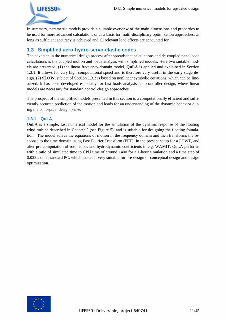
1.3 Simplified aero-hydro-servo-elastic codes
The next step in the numerical design process after spreadsheet calculations and de-coupled panel code
calculations is the coupled motion and loads analysis with simplified models. Here two suitable mod-
els are presented: (1) the linear frequency-domain model, QuLA is applied and explained in Section
1.3.1. It allows for very high computational speed and is therefore very useful in the early-stage de-
sign. (2) SLOW, subject of Section 1.3.2 is based on nonlinear symbolic equations, which can be line-
arized. It has been developed especially for fast loads analysis and controller design, where linear
models are necessary for standard control-design approaches.
The prospect of the simplified models presented in this section is a computationally efficient and suffi-
ciently accurate prediction of the motion and loads for an understanding of the dynamic behavior dur-
ing the conceptual design phase.
1.3.1 QuLA
QuLA is a simple, fast numerical model for the simulation of the dynamic response of the floating
wind turbine described in Chapter 2 (see Figure 5), and is suitable for designing the floating founda-
tion. The model solves the equations of motion in the frequency domain and then transforms the re-
sponse to the time domain using Fast Fourier Transform (FFT). In the present setup for a FOWT, and
after pre-computation of rotor loads and hydrodynamic coefficients in e.g. WAMIT, QuLA performs
with a ratio of simulated time to CPU time of around 1400 for a 1-hour simulation and a time step of
0.025 s on a standard PC, which makes it very suitable for pre-design or conceptual design and design
optimization.

D4.1 Simple numerical models for upscaled design
LIFES50+ Deliverable, project 640741 12/45
Figure 5: Sketch of the FOWT as implemented in QuLA
In the model, the floating wind turbine is simplified into two concentrated masses, mtop and mbot and
the tower. The top mass mtop includes the wind turbine rotor, hub and nacelle, while mbot refers to the
floating platform. The tower is modelled as a flexible Euler beam with distributed mass per length mt
and distributed bending stiffness EI, and is only allowed to bend according to its first fore-aft modal
shape. Four degrees of freedom are defined and solved for: floater surge , floater heave , floater
pitch around the floatation point and the elastic deflection at the tower top, . The time-domain
response of the floating wind turbine is governed by the equation of motion [7]:
( ) ( ) ∫ ( ) ( )
( ) ( ) (1)
Where M is the inertia matrix of the structure, A is the hydrodynamic added mass, the convolution
integral represents the linear radiation damping and C is the hydrostatic restoring matrix. F(t) is the
vector of external forcing of the four DOFs due to wind and waves, namely Faero and Fhydro. The vector
x(t) represents the motion in the different degrees of freedom. If harmonic motion is assumed, then
one can write the motion as x(t) = x(ω)eiωt
and the equation of motion can be written in frequency
domain:
( ( ( )) ( ) ) ( ) ( ) (2)
Here the added mass and damping matrices, A and B, depend on frequency. Once the equation is
solved in frequency domain, the response in the time domain can be obtained by inverse Fast Fourier
Transform (iFFT).

D4.1 Simple numerical models for upscaled design
LIFES50+ Deliverable, project 640741 13/45
1.3.1.1 Hydrodynamics
1.3.1.1.1 Wave kinematics
Under the assumption of inviscid, incompressible and irrotational flow, the linear Airy wave theory
provides a quick and simple estimation of the wave kinematics in constant water depth. Although
more complex wave theories could provide a more precise description of the flow, they would also
increase the computational cost, compromising the speed of the simple models. Thus, for the initial
phases of the design process, where efficiency is preferable over accuracy, linear Airy theory is ap-
plied.
1.3.1.1.2 Hydrodynamic loads
Given the geometry and size of the floating platform, a slender body approach and the consequent
application of the Morison equation for the hydrodynamic loads may not be sufficient. Instead, radia-
tion and diffraction effects must be included in the modelling of wave-structure interaction. For this
purpose, the commercial numerical tool WAMIT is employed. WAMIT solves the wave-structure
interaction in frequency domain by use of a potential flow panel method. For the present model, the
WAMIT tool is used to obtain the added mass and damping matrices A(ω) and B(ω), as well as the
hydrostatic restoring matrix C and the wave excitation forces Fexc(ω), due to incident wave (diffraction
and wave scattering). Inherent to potential flow methods, viscous effects are not included in the
WAMIT computations. Hence, empirically-determined viscous damping is added to the system
through the damping matrix B, and the viscous forcing in surge and heave directions is modelled
through the drag term in the Morison equation:
( ) ∫
( )| |
(3)
( )
( )| | (4)
where ρw is the water density, CD are the drag coefficients, D is the cylinder diameter, Ahp is the cross-
area of a heave plate, u and w are the horizontal and vertical wave velocities, and and denote the
structure velocities in surge and heave directions, respectively. The viscous forces are computed in the
time domain and transformed to the frequency domain. Hence, the total hydrodynamic force to be
included in the equation of motion would be:
( ) ( ) ( ) (5)
1.3.1.2 Aerodynamics
1.3.1.2.1 Wind field
The turbulent wind field for each wind speed is precomputed using TurbSim, an open-source numeri-
cal tool to create stochastic inflow turbulence, developed at the National Renewable Energy Laborato-
ry (NREL). The wind fields are created from a Kaimal spectrum, for a turbulence class C according to
the IEC-61400-3 standard. The grid, centered in the hub, spans 230 m and 33 points in the vertical and
horizontal directions, to ensure that the rotor area is well covered even when large platform motions
occur.

D4.1 Simple numerical models for upscaled design
LIFES50+ Deliverable, project 640741 14/45
1.3.1.2.2 Aerodynamic loads
In order to capture the complex rotor aerodynamics and at least some of the effects of the controller
while keeping the numerical model fast and simple, the aerodynamic loads and aerodynamic damping
are precomputed with FAST, an open-source integrated numerical tool developed at the National Re-
newable Energy Laboratory (NREL). For each wind speed, a simulation in turbulent wind is run with
rigid foundation and tower, and time series of aerodynamic loads are stored. Next, another simulation
is run for the same wind speed, where the platform pitch is enabled and an initial pitch displacement is
imposed. The amplitude of the hub displacement will decay in time due to the aerodynamic damping,
as seen in Figure 6 (left). The exponential decay of the peaks is used to compute the aerodynamic
damping for the given wind speed. The same procedure is repeated for different wind speeds and a
value of aerodynamic damping is extracted in each case (see Figure 6 (right)).
Figure 6: Free pitch decay test in wind (left) and aerodynamic damping as a function of wind speed (right)
The aerodynamic loads precomputed with FAST are applied to the simple model as Faero. The aerody-
namic damping is included in the equation of motion through the linear damping matrix B. However,
since the wind turbine controller was originally tuned for an onshore turbine, for wind speeds near or
above rated the pitch motion in the decay test will become unstable. Therefore, and as a temporary
solution until the controller for floating application is public, the aerodynamic damping for wind
speeds above 9 m/s was conservatively extrapolated from the values obtained for 5 and 7.1 m/s, as
seen in Figure 6.
1.3.1.3 Mooring system
The mooring system consists of 3 catenary lines, as specified in Section 1.3.1.3. In order to avoid solv-
ing the position of the catenary lines in time, the mooring system in the simple model is replaced by a
linear mooring matrix Cmoor, obtained at the equilibrium position and added to the original hydrostatic
restoring matrix C. Although a drastic simplification, the linearization of the mooring system provides
simplicity and speed to the simple model.
1.3.1.4 Setup of the model
In order to adapt the QuLA model to another floating wind turbine, one needs the following elements:
Hydrodynamic data such as hydrostatic, added mass and radiation damping matrices for the
given floating platform (computed with WAMIT or similar software)
Linearized mooring matrix for the given mooring configuration
D4.1 Simple numerical models for upscaled design
LIFES50+ Deliverable, project 640741 15/45
State-of-the-art model of the land-based wind turbine (in e.g. FAST) from which to extract the
aerodynamic loads and the aerodynamic damping
1.3.1.5 Calibration of the model
The simple model was calibrated against a FAST version of the same floating wind turbine. Time se-
ries of decay tests in surge, heave and pitch were produced with FAST and used as reference for cali-
bration. The natural frequencies were matched by adjusting the mooring matrix Cmoor, while the linear
damping matrix B was tuned to obtain the desired damping ratios. Further adjustment of the hydrostat-
ic matrix C was necessary in order to match the full aero-elastic model. For the present results, the
pitch diagonal element of the hydrostatic restoring matrix (C55) was reduced by 16% in order to match
the pitch natural frequency. It is expected that the cause of this need can be found by closer investiga-
tions.
1.3.2 SLOW
The simplified FOWT model SLOW (Simplified Low-Order Wind turbine) developed at the Universi-
ty of Stuttgart aims at a fast simulation of the overall nonlinear coupled dynamics. So far, simplified,
computationally efficient models allowing for numerous iterations at an early stage of development are
not possible with state-of-the-art, commercially available software. Simulation outputs to focus on
here are, e.g., the unconstrained 3D platform motion, rotor speed, blade pitch angle, tower top dis-
placement and main internal forces. With the linearized from of the equations of motion also the ei-
genvalues and eigenvectors can be analysed. Load distributions or specific node deflections of certain
bodies on the other hand are not sought to be covered by this model. The simplification also implies
that higher frequency modes of the stiffer DOFs like the blades or generator shaft are not considered.
From a numeric point of view focus is set on computational speed so that iterations, recursions, inte-
grations, excessive memory access, etc. is avoided wherever possible. In order to accomplish these
goals, the structure is modelled as a coupled multibody system of rigid bodies with only four DOFs.
The equations of motion (EQM) of the 3D model are set up by applying the Newton-Euler formalism.
As a result the mathematical model is available in state-space formulation as a system of symbolic
ordinary differential equations (ODE), which can be directly compiled, yielding a high computational
efficiency. Aerodynamics as well as the mooring line model is based on an interpolation of look-up
data that is gained in a pre-processing step. Aerodynamic coefficients allow the calculation of rotor
torque and thrust with a scalar rotor-effective wind speed as input. Quasi-static fairlead forces from the
mooring lines as a function of horizontal and vertical displacements are stored offline and interpolated
during runtime. Hydrodynamic forces are computed by the reduced model through a potential flow
approach.
The necessary pre-processing steps to run SLOW are (1) the identification of the force-RAO (wave
excitation force vector), the added mass and damping through a panel code. This calculation takes
roughly 10min per frequency-point with Ansys-Aqwa for the model used here. (2) The quasi-static
mooring force-discplacement relationship needs to be calculated which takes only seconds. (3) For the
calculation of the aerodynamic forces on the rotor disk the power and thrust coefficients have to be
calculated over tip-speed ratios (TSR) and blade pitch angles. This takes about three hours for the
model used here.
The simulation to CPU-time ratio has been determined for a 1-hour simulation with a fixed time-step
of 0.025s and a 4th order Runge-Kutta solver, it is about 160.
Table 2 shows the main characteristics of the model.
Table 2 - SLOW main properties
D4.1 Simple numerical models for upscaled design
LIFES50+ Deliverable, project 640741 16/45
Number of DOFs 4 (in this work)
Structural model Flexible multibody system, modally reduced bodies, floating
frame of reference. Nonlinear/linear
Hydrodynamic model Panel code (pre-processing) with constant added mass, linear
damping (in this work), state-space wave excitation force model
Aerodynamic model Look-up table of power- and thrust coefficient, nonlinear/linear,
relative, rotor-effective wind speed, blade-pitch-dependent
Mooring line model Nonlinear, quasi-static
Wind turbine controller Torque and pitch control
Sim. Time/CPU time 160
Programming C, Matlab
The next subsections will first introduce the set-up of the EQM of the structure and then addressing
the aero- and hydrodynamic subsystems.
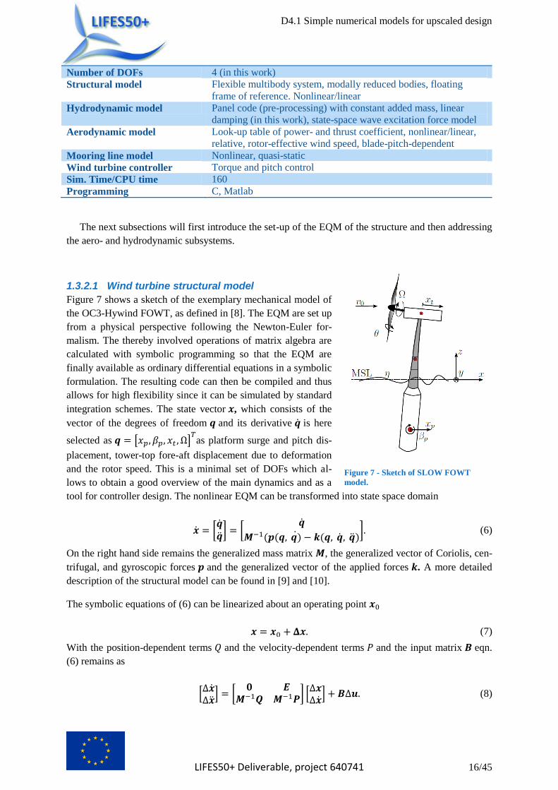
1.3.2.1 Wind turbine structural model
Figure 7 shows a sketch of the exemplary mechanical model of
the OC3-Hywind FOWT, as defined in [8]. The EQM are set up
from a physical perspective following the Newton-Euler for-
malism. The thereby involved operations of matrix algebra are
calculated with symbolic programming so that the EQM are
finally available as ordinary differential equations in a symbolic
formulation. The resulting code can then be compiled and thus
allows for high flexibility since it can be simulated by standard
integration schemes. The state vector , which consists of the
vector of the degrees of freedom and its derivative is here
selected as [ ] as platform surge and pitch dis-
placement, tower-top fore-aft displacement due to deformation
and the rotor speed. This is a minimal set of DOFs which al-
lows to obtain a good overview of the main dynamics and as a
tool for controller design. The nonlinear EQM can be transformed into state space domain
[
] [
( ( ) ( )] (6)
On the right hand side remains the generalized mass matrix , the generalized vector of Coriolis, cen-
trifugal, and gyroscopic forces and the generalized vector of the applied forces . A more detailed
description of the structural model can be found in [9] and [10].
The symbolic equations of (6) can be linearized about an operating point
(7)
With the position-dependent terms and the velocity-dependent terms and the input matrix eqn.
(6) remains as
[
] [
] [
] (8)
Figure 7 - Sketch of SLOW FOWT
model.

D4.1 Simple numerical models for upscaled design
LIFES50+ Deliverable, project 640741 17/45
The aerodynamic and mooring line forces are here also represented in a linear way. See [11] for de-
tails. In the following the nonlinear force models are presented.
1.3.2.2 Aerodynamic model
For this model BEM theory is avoided as this requires an iteration to find the induction factors. The
chosen procedure is to simulate a BEM model for various tip-speed ratios and blade pitch angles
until a steady state is reached as a pre-processing step, see Figure 8. With the resulting two-
dimensional look-up table for the thrust and torque coefficients and only the rotor effective wind
speed is necessary to calculate the thrust force and torque on the rotor. In order to com-
pute this representative wind speed at hub height first, a weighted average of the three-dimensional
turbulent wind field on the whole rotor plane is needed, given by . Second, a transformation of this
estimation into the rotor coordinate system is necessary, so that the relative horizontal wind speed is
computed. Finally, the relative rotor effective wind speed takes the form
(9)
This is the scalar disturbance necessary to calculate the thrust force
( )
(10)
and the external aerodynamic torque acting on the rotor body
( )
(11)
with air density and rotor radius . The described method has already been tested and successfully
implemented for nonlinear model predictive control (NMPC) in [12] .
Figure 8 – Example thrust and power coefficient look-up tables identified with AeroDyn [13].
1.3.2.3 Hydrodynamic model
The hydrodynamic model uses constant hydrodynamic coefficients for the added mass and damping.
( ( ) ( ) (12)
Morison equation is implemented but has not been enabled for the simulations presented here. The
wave excitation force is calculated based on the results of a panel code. The wave excitation force
results from an inverse Fourier transform of the wave spectrum multiplied by the frequency-dependent
wave excitation force vector (force-RAO) of the panel code.

D4.1 Simple numerical models for upscaled design
LIFES50+ Deliverable, project 640741 18/45
1.3.2.4 Mooring line model
The floating platform is moored by three catenary lines that are anchored on the seabed. The differen-
tial equation for a stationary line is solved analytically. According to [7] the resulting nonlinear system
of equations for the horizontal displacement and the vertical displacement of the fairleads with
the corresponding horizontal force and the vertical force has the form
( ) ( )
(13)
Applying a numerical solver, the forces on the fairleads can be obtained for various displacements
and . Eventually, a function interpolates this data and returns the external forces on the platform
body during runtime. Figure 9 shows the force-displacement lookup table.
Figure 9 – SLOW nonlinear quasi-static mooring forces.
Reference turbine and floating platform 2At the delivery date of this report the two public concepts of LIFES50+ have not yet been selected.
Therefore, WP 4 uses a generic platform concept together with the DTU10MW reference turbine, [3].
The generic platform concept has been developed by Task 4.3 of the project INNWIND.EU (2012-
2017), see [4].

D4.1 Simple numerical models for upscaled design
LIFES50+ Deliverable, project 640741 19/45
Figure 10 - DTU 10MW Reference Wind Turbine [3]
2.1 Platform The chosen platform is a semisubmersible platform with three concrete cylinders. The columns are
connected by a steel tripod which supports the tower of the DTU 10MW reference wind turbine. The
turbine tower has to be shortened by 25 m because of the height of the tripod and the column elevation
above sea water level (SWL). The hollow columns are filled with solid ballast. A detailed description
of the model can be found in INNWIND.EU deliverable D4.37, [4].
Figure 11 - Platform geometry.
Figure 11 shows the platform geometry. The concrete spar elevation above SWL is 10 m to avoid
green water loads on the steel structure. The column radii are of 15m and the column distance to the
vertical centerline is 26m (Figure 11). The wall thickness of the concrete columns was set to 0.4 m.
The detailed platform properties are collected in Table 3. The advantages of this concept are the low
material cost due to easily manufacturable concrete columns with only one interface at their top, above
water level. The draft can be adjusted to the selected site and also the installation strategy can be se-
lected according to the available facilities. For low drafts the turbine can be installed in the harbour.

D4.1 Simple numerical models for upscaled design
LIFES50+ Deliverable, project 640741 20/45
In order to assess the sensitivities of this concept towards material cost and dynamic properties
(RAOs) a parametric design approach starting with conceptual spreadsheet calculations up to panel
code calculations has been done. This approach is detailed in Section 1.1. The generic concept has
been developed specifically for research and optimization studies.
Figure 12 – Two example design of generic TripleSpar concept.
Table 3 - TripleSpar properties.
Platform
Draft 54.46 m
Elevation of tower base
above SWL
25 m
Water displacement 29 205.09 m3
Center of mass below
SWL
36.02 m
Center of buoyancy below
SWL
27.54 m
Platform mass 28 230 t
Ballast mass 17 264 t
columns
Length 65 m
Distance to the center 26 m
Diameter 15 m
Elevation above SWL 10.5 m
Heave plates
Thickness 0.5 m
Diameter 22.5m
Mass 678.7t
Tripod
Total height 15 m
Height outer cylinder 11 m
Diameter outer cylinder 5.64 m
Bar cross-section width 5.64 m
Wall thickness 0.056 m
Mass 971.3 t
DTU 10MW RWT Tower height above SWL 119 m
Reduced tower length to 94 m

D4.1 Simple numerical models for upscaled design
LIFES50+ Deliverable, project 640741 21/45
hub height
Rotor diameter 178.3 m
Rotor mass 228 t
Nacelle mass 446 t
Reduced tower mass 433 t
I11 about turbine CM 1.613e9 kgm2
I22 about turbine CM 1.613e9 kgm2
I33 about turbine CM 0.491e9 kgm2
Densities
Concrete density 2 750 kg/m3
Steel density 7 750 kg/m3
Ballast density 2 500 kg/m3
Water density 1 025 kg/m3
Total platform mass 28268.22 t
Moments of Inertia about
center of mass
Platform I11 without tur-
bine
1.8674e10 kgm2
Platform I22 without tur-
bine
1.8674e10 kgm2
Platform I33 without tur-
bine
2.0235e10 kgm2
FOWT System I11 3.907e10 kgm2
FOWT System I22 3.907e10 kgm2
FOWT System I33 3.1129e10 kgm2
Hydrostat-
ics/Hydrodynamics
Heave stiffness C33 5.321e6 N/m
Pitch stiffness C55 2.922e9 Nm/rad
Pitch stiffness C55
w/o gravitation (FAST)
-6.199e9Nm/rad
2.2 Mooring system A catenary mooring system is utilized for station-keeping of the platform. It consists of three lines,
with one line per platform column and two upwind lines. The line is connected to a fairlead that ex-
tends radially from the column and has a portion lying on the seabed to ensure there are no vertical
forces on the anchor in ultimate limit state conditions. Figure 13 depicts the configuration of a single
mooring line and Table 4 provides the relevant information concerning the mooring system. Table 5
and Table 6 provide the linearized mooring system stiffness matrices at equilibrium and at rated wind
speed positions, respectively, which are used within QuLA and the linear version of SLOW. Details of
the mooring design can be found in [14].

D4.1 Simple numerical models for upscaled design
LIFES50+ Deliverable, project 640741 22/45
Figure 13 – Left: mooring line configuration, right: mooring system orientation
Table 4 - Mooring system parameters
Parameter Unit
Number of lines - 3
Line type - Steel chain
Line mass in air kg/m 594.00
Line mass in water kg/m 516.59
Chain diameter m 0.18
Hydrodynamic chain diameter m 0.31
Un-stretched line length m 610.00
Extensional stiffness N 1.3739e+09
Fairlead radius m 54.48
Anchor radius m 600.00
Vertical fairlead distance above MSL m 8.70
Vertical anchor distance below MSL m 180.00
Table 5 - Linearized mooring system stiffness matrix at equilibrium position [N/m]/[Nm/rad]
1 2 3 4 5 6
1 -8,3283E+04 4,0571E-05 5,8208E-11 5,6087E-03 -2,8465E+06 6,3033E-07
2 -3,2045E-05 -8,3283E+04 1,1642E-10 2,8455E+06 0,0000E+00 3,6908E-07
3 3,5123E+00 3,7591E-05 -5,7337E+04 4,6545E-03 9,3746E+02 0,0000E+00
4 1,2370E-03 2,8436E+06 0,0000E+00 -1,9999E+08 1,4230E-07 3,2756E-04
5 -2,8436E+06 1,3773E-03 -3,7253E-09 1,8942E-01 -2,0002E+08 -5,672E-04
6 -5,5507E-07 7,6525E+01 0,0000E+00 -1,5652E+05 0,0000E+00 -2,693E+08
Table 6 - Linearized mooring system stiffness matrix at rated wind speed position [N/m]/[Nm/rad]
1 2 3 4 5 6
1 -7,6888E+04 9,6709E-04 -2,2646E+04 -9,0522E-04 -2,5166E+06 -3,309E-02

D4.1 Simple numerical models for upscaled design
LIFES50+ Deliverable, project 640741 23/45
2 3,8181E-03 -1,2583E+05 -6,6702E-03 3,9710E+06 4,4467E-09 -9,747E+04
3 -2,2613E+04 7,3521E-04 -5,9279E+04 4,6391E-03 -5,9261E+05 -2,068E-02
4 -1,2496E-01 3,9680E+06 2,1934E-01 -2,8004E+08 1,4230E-07 4,4389E+07
5 -2,5152E+06 2,8448E-02 -5,9427E+05 1,1805E-01 -1,6750E+08 -1,257E+00
6 7,8451E-03 -9,6254E+04 -1,3039E-02 -6,7942E+06 -7,1148E-08 -3,076E+08
2.3 Wind turbine The DTU 10MW Reference Wind Turbine [3], depicted in Figure 10, is installed on the Triple Spar
platform. To account for the freeboard of the platform and to maintain the same hub height the turbine
tower was shortened from 115.63 metres to 90.63 metres. This was done by removing the bottom 25
metres of the original tower as detailed by [4]. The influence of this was to increase the tower bending
natural frequencies, possibly into the operating 3P range, and should be evaluated further in the con-
ceptual substructure development. However this was not investigated in detail here as the scope of this
report is to compare numerical models simulating a reference floating wind turbine design.
2.4 Controller The DTU10MW reference turbine is here installed on a floating platform. Therefore, the baseline con-
troller cannot be used here due to the “negative damping” problem, which has been reported in the
literature, see e.g. [15], [16], [17]. In LIFES50+ a controller will be developed for a floating founda-
tion by DTU. However, this controller was not available before the delivery date of the present report.
Therefore, a conceptual controller has been developed at the University of Stuttgart in order to be able
to compare responses at above-rated operational wind conditions. In this section a preliminary control-
ler is designed using a coupled linear model for the above-rated controller and the below-rated control
concept adapted from the NREL 5MW RWT [18]. For the purpose of designing a simple conceptual
controller a single-input-single-output (SISO) Proportional-Integral (PI) controller was chosen, see
Figure 14. It has been designed using the linearised SLOW model following the method reported in
[11]. The design strategy is based on the platform pitch mode: Its pole in the closed loop is set such
that its real part is at -0.005 in the left-half plane for all wind speeds. This method results in a gain-
scheduling which ensures the stability of the platform at all operating conditions. With this platform
pitch mode close to the imaginary axes a good performance of the drivetrain mode is ensured since
this mode becomes more stable for increasing gains, which, in turn, lead to instability of the platform,
see Figure 16. Figure 15 shows that for two large gains there appears a right-half-plane zero next to the
platform pitch mode. For more details see [11].
Figure 17 shows the gain scheduling of the proportional gain of the controller. The time constant is
s, the generator torque is constant in region 3 (above rated wind speeds).
In the SLOW and FAST model a linear 2nd
-order actuator model has been used with a natural frequen-
cy of 1.6Hz and a damping ratio of 0.8.

D4.1 Simple numerical models for upscaled design
LIFES50+ Deliverable, project 640741 24/45
Figure 14 – Conceptual blade-pitch controller.
Figure 15 – Closed-loop bode plots from wind speed to rotor speed.

D4.1 Simple numerical models for upscaled design
LIFES50+ Deliverable, project 640741 25/45
Figure 16 – Closed-loop pole-zero map.
Figure 17 – Gain scheduling of conceptual controller.
Selection of Load Cases 3A set of simplified, unidirectional load cases is chosen in order to compare the performance of the
simple models presented in this document. First, a number of system-identification load cases is se-
lected. This set is derived from the code-comparison projects OC3, OC4 and OC5, see, e.g., [8], [19]
and [20]. Especially for model verification these free-decay cases and cases with only wind or only
waves are very useful. In this study the simplified models is compared to a common FAST [21] mod-
el, see [22] for a description of the model setup. These cases are shown in this report in order to show
the agreement of the simple models compared to the reference model FAST in this system identifica-
tion environment. This allows to better interpreting the results of the design load cases (DLC) in op-
erational and extreme conditions.
3.1 System identification These cases are necessary in the pre-design phase or every time a new numerical model is set up. It
serves for verification of the new setup for plausibility.

D4.1 Simple numerical models for upscaled design
LIFES50+ Deliverable, project 640741 26/45
Table 7 - Description of cases for system identification
Static
equilibrium
Free decay in
surge
Free decay in
heave
Free decay in
pitch
Response to
deterministic
waves
A case with no
wind or waves, to
ensure the struc-
ture can remain in
equilibrium in
absence of exter-
nal loads.
A case with no
wind or waves,
where the initial
surge displace-
ment is +22 m.
A case with no
wind or waves,
where the initial
heave displace-
ment is +6 m.
A case with no
wind or waves,
where the initial
pitch displace-
ment is +8 deg.
Response to a
deterministic
regular wave with
wave height H=6
m and wave peri-
od T=10 s.
3.2 Design load cases Six load cases were selected for this study, in which all considered unidirectional wind and wave con-
ditions to ensure fast evaluation.
3.2.1 Fatigue loads during operation
A set of load cases belonging to DLC1.2, with normal turbulence class C and normal sea states, for the
combinations ( , ) given in the design basis of LIFES50+ [5] (Table 19) was applied. There are
three wave conditions for every wind speed with a different probability of occurrence. The conditions
with the smallest peak spectral period are here denoted A, and the subsequent ones B and C in the
following.
Table 8 - Environmental conditions for DLC 1.2, extracted from D7.2 [5].
Vhub Hs Tp Probability
[m/s] [m] [s]
5 1.38 7 6.89%
5 1.38 11 3.45%
7.1 1.67 5 5.99%
7.1 1.67 8 11.98%
7.1 1.67 11 5.99%
10.3 2.2 5 6.41%
10.3 2.2 8 12.83%
10.3 2.2 11 6.41%
13.9 3.04 7 5.12%
13.9 3.04 9.5 10.24%
13.9 3.04 12 5.12%
17.9 4.29 7.5 2.90%
17.9 4.29 10 5.81%
17.9 4.29 13 2.90%
22.1 6.2 10 0.94%
22.1 6.2 12.5 1.88%
22.1 6.2 15 0.94%
25 8.31 10 0.19%
25 8.31 12 0.37%
25 8.31 14 0.19%
5 1.38 7 6.89%
5 1.38 11 3.45%
7.1 1.67 5 5.99%
7.1 1.67 8 11.98%

D4.1 Simple numerical models for upscaled design
LIFES50+ Deliverable, project 640741 27/45
3.2.2 Ultimate loads during operation
A set of load cases belonging to DLC1.6, with normal turbulence class C and severe sea states, for the
combinations ( , ) given in Table 9 was applied. The chosen periods are all below the natural
periods of the system.
Table 9 - Environmental conditions for DLC 1.6.
Vhub Hs Tp
[m/s] [m] [s]
5 15.6 12
5 15.6 14
5 15.6 16
5 15.6 18
7.1 15.6 12
7.1 15.6 14
7.1 15.6 16
7.1 15.6 18
10.3 15.6 12
10.3 15.6 14
10.3 15.6 16
10.3 15.6 18
13.9 15.6 12
13.9 15.6 14
13.9 15.6 16
13.9 15.6 18
17.9 15.6 12
17.9 15.6 14
17.9 15.6 16
17.9 15.6 18
22.1 15.6 12
22.1 15.6 14
22.1 15.6 16
22.1 15.6 18
25 15.6 12
25 15.6 14
25 15.6 16
25 15.6 18
3.2.3 Extreme waves with parked turbine
Parked or idling turbine, m/s and extreme sea state with Hs=15.6 m and Tp=12, 14, 16 and 18
s.
3.2.4 Extreme wind gust with operating turbine
Wind with extreme operational gust (EOG) and normal sea state.
Results 4The results of the simplified coupled dynamic models described in Section 1.3 are compared to each
other to evaluate their applicability. Here, the suitability of the models in different design load cases
can be evaluated. The results have been compared to the state-of-the-art tool FAST v8 that has been
set up for the LIFES50+ project with the DTU 10MW RWT in [22], see [23]. It should be noted that
the results above rated wind speed rely on an ad-hoc controller designed specifically for the present

D4.1 Simple numerical models for upscaled design
LIFES50+ Deliverable, project 640741 28/45
deliverable. Changes to the results above and close to rated wind speed can thus be expected following
implementation of a refined controller.
The figures in this chapter have a consistent line style convention for the three different models,
QuLA, SLOW and FAST. Additionally, in some figures the linearized version of SLOW has been
included. The line styles are summarized in Table 10. The plotted signals include the platform surge
displacement at the SWL, , the platform pitch displacement, , the tower-top displacement, , as
well as the blade pitch angle, , and the rotor speed, . The rotor-effective wind speed and the
wave height and the tower-base bending moment about the axis perpendicular to the wind speed
are shown.
Table 10 - Results line style convention
Model Line style
QuLA blue
SLOW (nonlinear) red
FAST yellow
SLOW (linearized) purple
4.1 System identification
In this section the results of the first identification tests described in Chapter 3 are shown.
4.1.1 Eigenanalysis
Table 11 shows an Eigenanalysis of the coupled FOWT without controller (open loop). It has been
made with SLOW and QuLA. Since SLOW has in the setup used here no heave DOF that one is only
shown for QuLA. The drivetrain mode is overdamped in the open-loop case (without active controller)
and is therefore not shown.
Table 11 – Eigenanalysis, no aerodynamic forces.
Undamped eigen-
frequency
Undamped eigenperiods
Model QuLA SLOW FAST QuLA SLOW
[Hz] [Hz] [s] [s] Difference
to FAST
[%]
[s] Difference to
FAST [%]
Platform
surge
0.0058 0.0054 174.0 172.4 0.92 185.19 6.43
Platform
heave
0.0599 - 16.7 16.69 0.06 - -
Platform
pitch
0.0398 0.0395 26.47 25.13 5.06 25.32 4.34
Tower-top
fore-aft
displace-
ment
0.4157 0.4065 2.56 2.41 5.86 2.46 3.91
4.1.2 Time-domain
In order to assess transient responses of the structure and the applied models, time-domain simulations
are performed and compared to FAST results. These include free-decay simulations, regular wave
response and the response to an extreme operational gust (EOG). The free-decay simulations are per-
formed in still water without aerodynamic forcing of the simplified tools QuLA and SLOW and the
reference model FAST, see Figure 18 and Figure 19.

D4.1 Simple numerical models for upscaled design
LIFES50+ Deliverable, project 640741 29/45
Surge decay simulation. As indicated by the eigenanalysis above, the surge natural frequency of
SLOW and QuLA is in very good agreement with the FAST surge natural frequency. In the first surge
oscillation, Figure 18, the simplified models appear to be less damped than the FAST model. However
in subsequent surge oscillations the opposite is true, in particular for QuLA. This is evidence of the
nonlinear hydrodynamic viscous damping model utilized in FAST as compared to the linear models
used in QuLA and SLOW. The induced pitch motion predicted by all three models are in good agree-
ment. This indicates that couplings between surge and pitch are sufficiently captured by the simplified
models. The slight difference in steady state pitch offset is due to the fact that in QuLA the lateral
eccentric position of the wind turbine centre of gravity is not considered.
Pitch decay simulation. In the case of pitch decay, Figure 19, similar observations as in surge can be
made. In this case there are slightly larger discrepancies between the simplified models and FAST
predicted oscillation peaks, which in turn exacerbates the differences in induced surge motion between
the models. However these differences are not large and the behaviour of the simplified models in
pitch is comparable to the FAST model. The tower-top displacement is less damped for SLOW and
QuLA. However, in these simulations no aerodynamic forces are present. These will introduce a
damping much larger than the structural damping.
Regular wave simulation. Figure 20 shows the response to regular waves of s. QuLA predicts
here slightly larger amplitudes in surge and pitch. The wave excitation force models are essentially the
same for the three models. All read the frequency-domain wave excitation force vector from WAMIT
and convert it to time-domain through an inverse Fourier transform. The larger response of QuLA may
be explained by the absence of quadratic viscous damping.
Extreme Operating Gust. The response to an Extreme Operating Gust (EOG) in still water serves well
for model verification as it excites the system once, resulting in a decay response of the system. It is
shown for the FAST model and the nonlinear and the linearized SLOW model in Figure 21 for 16m/s
wind speed. The linearized SLOW model is very useful for so called single-in-single-out (SISO)-
control design methods but due to the nonlinearities of the aerodynamic forces and also the structural
equations of motion the linearization poses difficulties. The results show that the response compares
well between the models. Therefore, the structural modes of the tower, the aerodynamic model, the
still-water hydrodynamics and the mooring dynamics can be considered valid also for the linear model
and applicable for controller design. The linear model has been used for the design of the controller,
see Section 2.4.

D4.1 Simple numerical models for upscaled design
LIFES50+ Deliverable, project 640741 30/45
Figure 18 – Surge free-decay.
Figure 19 – Pitch free-decay..

D4.1 Simple numerical models for upscaled design
LIFES50+ Deliverable, project 640741 31/45
Figure 20 – Regular wave response.
Figure 21 – Linear SLOW model compared to nonlinear and FAST in EOG @ 16m/s.
4.2 Design load cases
The design load cases (DLC) presented in this section are taken from the design basis of LIFES50+
[5]. A selection has been made for this deliverable with a complete operational load case for fatigue
analysis and several operational and shut-down conditions for extreme-load analysis. For all design

D4.1 Simple numerical models for upscaled design
LIFES50+ Deliverable, project 640741 32/45
load cases 1-hour simulations have been performed, where the transient of the first 10min has been cut
off for the calculation of statistical values and DELs.
4.2.1 Fatigue loads
In this section DLC 1.2 is evaluated. One above-rated wind speed case has been selected for a time-
domain comparison of FAST, SLOW and QuLA, see Figure 22. It can be seen that the magnitudes
compare well between the models but also some of the transient features are followed well by the
models. The same wave train and wind field has been used for all models.
Figure 22 – DLC1.2 time domain comparison 18m/s, Hs=4.3m, Tp=10s.
The difference in response can be explained by the different aerodynamic forcing approaches of the
models, see Section 1.3. For a frequency-domain assessment the power-spectral density (PSD) is cal-
culated for the same case of DLC1.2 as for the time-domain comparison, see Figure 24 and for a be-
low-rated case with a different wave peak-spectral period, Figure 23. It shows that for low frequencies
the models compare well with the platform surge and pitch modes at 0.005Hz and 0.04Hz. It can be
seen that SLOW does not capture the correct magnitude response around the tower mode (0.4Hz). This
is due to the fact that the rotor-effective wind speed is used as input to the model, which filters most of
the high-frequency turbulence and therefore the tower-mode is not excited in the same way as in
FAST. Also the 3p-frequency at 0.48Hz, slightly above the tower eigenfrequency, is not visible for
SLOW as the blades are not modelled and effects from e.g. wind shear. QuLA does capture well the
3p-excitation, which is due to the fact that the thrust force timeseries are captured from an onshore
simulation with FAST. It shows that although this procedure is not completely “coupled” these effects
can be well represented. The first tower frequency is estimated well by QuLA, although the energy
content is here overestimated. Furthermore, the damping of QuLA seems to be smaller than in the
other models, leading to larger peaks around the tower frequencies in the PSD plot.

D4.1 Simple numerical models for upscaled design
LIFES50+ Deliverable, project 640741 33/45
Figure 23 – DLC1.2 PSD comparison tower-top displacement 10m/s, Hs=2.2m, Tp=8s.
Figure 24 – DLC1.2 PSD comparison tower-top displacement 18m/s, Hs=4.3m, Tp=10s.
The damage equivalent loads of the tower-top fore-aft displacement are compared for three different
wave environments as specified in the LIFES50+ design basis [5]. Figure 25, Figure 26 and Figure 27
show a comparison between QuLA, SLOW and FAST over wind speeds for the three wave conditions,
shown in Table 8. It can be seen that QuLA overpredicts for most bins, whereas SLOW underpredicts
the DELs. One reason for the underprediction of SLOW is the filtering of the high-frequency turbu-
lence in the rotor-effective wind speed as mentioned above. QuLA shows also in the PSD plots above
a higher amplitude around the tower eigenfrequency, which might explain the higher DELs compared
to FAST.

D4.1 Simple numerical models for upscaled design
LIFES50+ Deliverable, project 640741 34/45
Figure 25 – DLC1.2 tower-base DEL comparison over wind speeds, wave condition A
Figure 26 – DLC1.2 tower-base DEL comparison over wind speeds, wave condition B

D4.1 Simple numerical models for upscaled design
LIFES50+ Deliverable, project 640741 35/45
Figure 27 – DLC1.2 tower-base DEL comparison over wind speeds, wave condition C
In a second step the DELs have been weighted with the probability density shown in Table 8 and aver-
aged for the three wave conditions. Figure 28 shows that the weighting stresses wind speeds around
rated due to the higher probability of occurrence of these wind speeds.
Figure 28 – DLC1.2 weighted tower-base DEL, averaged over wave A, B, C.
The probability of exceedance by the three models is compared in Figure 29 for wave A and C. The
timeseries of the considered signals have been binned based on the zero-upcrossing periods of the
wave height signals and the extremes recorded and plotted over their probability of exceedance. Figure
29 shows the platform surge and Figure 30 the tower-top displacement signal. In both figures three
wind bins of m/s for wave environments A and C have been compared. Only around
rated (10m/s) QuLA predicts smaller extreme values. While SLOW compares well to FAST at
m/s, notable discrepancies occur between FAST and the simplified models in particular for
m/s and also at m/s for wave climate C.

D4.1 Simple numerical models for upscaled design
LIFES50+ Deliverable, project 640741 36/45
Figure 29 – DLC1.2 platform surge probability of exceedance; wave A, C; v=[10,18,25]m/s; (QuLA-blue,
SLOW-red, FAST-yellow).
For the tower-top fore-aft probability of exceedance in Figure 30 one can see a comparable picture to
the DEL plots of Figure 28. QuLA overpredicts the amplitudes whereas SLOW underpredicts them.
The probability of exceedance calculation is usually useful for extreme value calculation. However,
the plots have been produced here also for a production load case in order to compare them to the ex-
treme load cases in the following. It is mentioned that the motion and load amplitudes assessed in this
method depend strongly on the damping. Since SLOW and QuLA only consider linear hydrodynamic
damping a large difference appears here although the general dynamics agree. It is again stressed that
results above rated wind speed rely on the controller. Hence although model re-calibration is needed to
improve the match to the FAST model, the results will also change once the LIFES50+ controller is
available in the project.

D4.1 Simple numerical models for upscaled design
LIFES50+ Deliverable, project 640741 37/45
Figure 30 - DLC1.2 tower-top fore-aft probability of exceedance; wave A, C; v=[10,18,25]m/s (QuLA-blue,
SLOW-red, FAST-yellow).
4.2.2 Extreme loads
For extreme wave conditions the operational load case DLC1.6 has been considered with 1-hour simu-
lations of each case, resulting in 7 wind speed bins and four wave scenarios and therefore 28 simula-
tions. These conditions are for the most severe site considered in LIFES50+, that of West of Barra.
Figure 31 shows the exceedance probability of platform surge displacement for QuLA, SLOW and
FAST. For the large-period case C SLOW overpredicts the motion for wind speed m/s as was
seen also above. QuLA overpredicts here the probability for most excursions, although especially for
the tower-top displacement the agreement is acceptable.

D4.1 Simple numerical models for upscaled design
LIFES50+ Deliverable, project 640741 38/45
Figure 31 - DLC1.6 platform surge probability of exceedance; wave A, C; v=[10,18,25]m/s (QuLA-blue,
SLOW-red, FAST-yellow).
Figure 32 shows the tower-top probability of exceedence of DLC1.6. It can be seen that generally
QuLA overpredicts the displacements compared to FAST, whereas SLOW underpredicts them. Again,
the results show the ability of the simplified models to predict the correct magnitude of the response,
even in a harsh environment. More model tuning can very likely increase the level of accuracy and
will be pursued in future work.

D4.1 Simple numerical models for upscaled design
LIFES50+ Deliverable, project 640741 39/45
Figure 32 - DLC1.6 tower-top fore-aft probability of exceedance; wave A, C; v=[10,18,25]m/s (QuLA-blue,
SLOW-red, FAST-yellow).
Figure 33 shows the probability of exceedance of DLC6.1 where the rotor is idling. The rotor models
of FAST and SLOW have been configured such that a viscous brake at the shaft is active and no ex-
cessive blade loads occur. It can be seen that there are large discrepancies between the models, which
is due to the absence of nonlinear damping in the simple models. For a reliable capturing of the re-
sponse at these harsh wave environments the models need to be augmented by a more realistic damp-
ing model. The first improvement in this regard will be a representation of quadratic viscous damping
in QuLA.

D4.1 Simple numerical models for upscaled design
LIFES50+ Deliverable, project 640741 40/45
Figure 33 - DLC6.1 platform pitch and tower-top fore-aft probability of exceedance; Tp=[12,18]s (QuLA-
blue, SLOW-red, FAST-yellow).
Conclusions 5The design approach for floating wind turbine substructures considered in this work package promotes
utilizing a set of different numerical models covering a range of fidelity and computational efficiency.
This report has presented the formulation and assessment of parametric and simplified numerical de-
sign tools for use within the conceptual design stage of floating substructures for 10MW wind tur-
bines. SLOW, developed at USTUTT, is a nonlinear coupled numerical model for carrying out fast
simulations in the time domain and is particularly aimed at very early design of the floating substruc-
ture and wind turbine controller. QuLA, developed at DTU, is a coupled numerical model for evaluat-
ing the dynamic response of the floating wind turbine in the frequency domain, with a scope to be
more computationally efficient than time-domain simplified numerical models.
The DTU 10MW reference wind turbine installed on the Triple Spar concept was considered as a case
study in this work for evaluating a subset of DLCs established in the LIFES50+ Design Basis for the
West of Barra site. This site was chosen as it represented the harshest environment available within the
LIFES50+ project. Simulations were also carried out using a state-of-the-art FAST model of the float-
ing wind turbine, and were used as a benchmark for results from the simplified numerical models.

D4.1 Simple numerical models for upscaled design
LIFES50+ Deliverable, project 640741 41/45
It was found that the simplified models were capable of predicting fatigue performance in operating
conditions. However, in extreme conditions the simplified numerical models were in limited agree-
ment with the state-of-the-art FAST model. Notable differences were observed, and these are attribut-
ed to differences in control, damping and mooring system models within the simplified numerical
design tools. Capturing damping related to floating wind turbine aerodynamics is not trivial and as yet
no method has been established. The addition of quadratic hydrodynamic damping would contribute to
improved performance in extreme conditions. Further, moving beyond a constant-coefficient stiffness
matrix to represent the mooring system within QuLA would also contribute to better predicting the
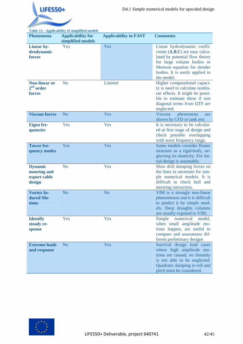
dynamic response of the floating wind turbine in extreme conditions. Table 12 presents an overview of
the observations made in this work on the applicability of the simplified models for a number of phe-
nomena.
The simplified numerical design tools presented here have the potential to be improved such that their
applicability in predicting extreme responses is achieved. This is the subject of future work in work
package 4, where advanced numerical tools and experimental results will be used to improve such
simplified numerical design tools.
D4.1 Simple numerical models for upscaled design
LIFES50+ Deliverable, project 640741 42/45
Table 12 - Applicability of simplified models
Phenomena Applicability for
simplified models
Applicability in FAST Comments
Linear hy-
drodynamic
forces
Yes Yes Linear hydrodynamic coeffi-
cients (A,B,C) are easy calcu-
lated by potential flow theory
for large volume bodies or
Morison equation for slender
bodies. It is easily applied in
the model.
Non-linear or
2nd
order
forces
No Limited Higher computational capaci-
ty is need to calculate nonlin-
ear effects. It might be possi-
ble to estimate these if non
diagonal terms from QTF are
neglected.
Viscous forces No Yes Viscous phenomena are
shown by CFD or tank test
Eigen fre-
quencies
Yes Yes It is necessary to be calculat-
ed at first stage of design and
check possible overlapping
with wave frequency range.
Tower fre-
quency modes
Yes Yes Some models consider floater
structure as a rigid-body, ne-
glecting its elasticity. For ini-
tial design is assumable.
Dynamic
mooring and
export cable
design
No Yes Slow drift damping forces on
the lines in uncertain for sim-
ple numerical models. It is
difficult to check hull and
mooring interaction.
Vortex In-
duced Mo-
tions
No No VIM is a strongly non-linear
phenomenon and it is difficult
to predict it by simple mod-
els. Deep draughts columns
are usually exposed to VIM.
Identify
steady re-
sponse
Yes Yes Simple numerical model,
when small amplitude mo-
tions happen, are useful to
compare and assesassess dif-
ferent preliminary designs
Extreme loads
and response
No Yes Survival design load cases
where high amplitude mo-
tions are caused, no linearity
is not able to be neglected.
Quadratic damping in roll and
pitch must be considered.

D4.1 Simple numerical models for upscaled design
LIFES50+ Deliverable, project 640741 43/45
Bibliography 6
[1] Goren Aguirre and Joannès Berque, "LIFES50+ D7.3: Survey of FOWT Design Practice and Gap
Analysis," Tecnalia Foundation, 2015.
[2] Kolja Müller et al., "LIFES50+ D7.4: State-of-the-Art FOWT design practice and guidelines,"
University of Stuttgart, 2016.
[3] Christian Bak et al., "Description of the DTU 10 MW Reference Wind Turbine," DTU, Tech.
rep..
[4] Frank Lemmer, José Azcona, Florian Amann, and Feike Savenije, "INNWIND.EU D4.37 Design
Solutions for 10MW Floating Offshore Wind Turbines," INNWIND.EU, 2016.
[5] Antonia Krieger, Gireesh Ramachandran, Luca Vita, Pablo, Berque, Joannès Gómez Alonso, and
Goren Aguirre, "LIFES50+ D7.2: Design Basis," DNV-GL, 2015.
[6] Michael Borg and Henrik Bredmose, "LIFES50+ Deliverable 4.4: Overview of the numerical
models used in the consortium and their qualification," DTU Wind Energy, 2015.
[7] Jason Jonkman, "Dynamics Modeling and Loads Analysis of an Offshore Floating Wind
Turbine," Ph.D. dissertation 2007.
[8] Jason Jonkman, "Definition of the Floating System for Phase IV of OC3," NREL, Tech. rep.
2010.
[9] Frank Sandner, David Schlipf, Denis Matha, Robert Seifried, and Po Wen Cheng, "Reduced
Nonlinear Model of a Spar-Mounted Floating Wind Turbine," in DEWEK, Bremen, Germany,
2012. [Online]. http://elib.uni-
stuttgart.de/opus/volltexte/2013/8439/pdf/Sandner_ReducedModel_Dewek2012.pdf
[10] Denis Matha, Frank Sandner, and David Schlipf, "Efficient critical design load case identification
for floating offshore wind turbines with a reduced nonlinear model," , vol. 555, dec 2014.
[Online]. http://stacks.iop.org/1742-
6596/555/i=1/a=012069?key=crossref.2cf58ea90e06a51553c9c6441bd0248d
[11] Frank Lemmer, Steffen Raach, David Schlipf, and Po Wen Cheng, "Prospects of Linear Model
Predictive Control on a 10MW Floating Wind Turbine," in Proceedings of the ASME 34th
International Conference on Ocean, Offshore and Arctic Engineering, St. John's/Canada, 2015.
[Online]. http://elib.uni-stuttgart.de/opus/volltexte/2015/9895/
[12] David Schlipf et al., "Nonlinear Model Predictive Control of Floating Wind Turbines," , 2013, pp.
1-9. [Online]. http://elib.uni-stuttgart.de/opus/volltexte/2013/8516/pdf/13TPC_987Schlipf.pdf
[13] Hansen Craig and David J. Laino, "User's Guide to the Wind Turbine Aerodynamics Computer
Software AeroDyn," Tech. rep..
[14] Michael Borg, "Mooring system analysis and recommendations for the INNWIND Triple Spar
concept.," Technical University of Denmark, Lyngby, Denmark, DTU Wind Energy Report-I-
D4.1 Simple numerical models for upscaled design
LIFES50+ Deliverable, project 640741 44/45
0448 2016.
[15] T. J. Larsen and T. D. Hanson, "A method to avoid negative damped low frequent tower
vibrations for a floating, pitch controlled wind turbine," Journal of Physics: Conference Series,
75, 012073. doi:10.1088/1742-6596/75/1/012073,.
[16] Gijs Van Der Veen, Yan Couchman, and Robert Bowyer, "Control of floating wind turbines," in
Proceedings of the American Control Conference ACC, 2012, pp. 3148-3153.
[17] Boris Fischer, "Reducing rotor speed variations of floating wind turbines by compensation of
non-minimum phase zeros," , EWEA 2012, 2012.
[18] Jason Jonkman, S Butterfield, W Musial, and G Scott, "Definition of a 5-MW Reference Wind
Turbine for Offshore System Development," NREL, Boulder/USA, 2009.
[19] Amy Robertson et al., "Definition of the Semisubmersible Floating System for Phase II of OC4,"
Tech. rep..
[20] Amy Robertson, "Introduction to the OC5 Project," in EERA Deepwind, Trondheim/NO, 2015.
[Online]. http://www.sintef.no/Projectweb/Deepwind_2015/Presentations/
[21] Jason Jonkman and Bonnie Jonkman. (2016, March) NWTC Information Portal (FAST v8).
[Online]. https://nwtc.nrel.gov/FAST8
[22] Michael Borg, Mahmood Mirzaei, and Henrik Bredmose, "LIFES50+ D1.2 Wind turbine models
for the design," 2016.
[23] Michael Borg, "Generic floating substructure configuration and numerical models for wind
turbine controller tuning in LIFES50+," Technical University of Denmark, Lyngby, Denmark,
DTU Wind Energy Report-I-0449 2016.
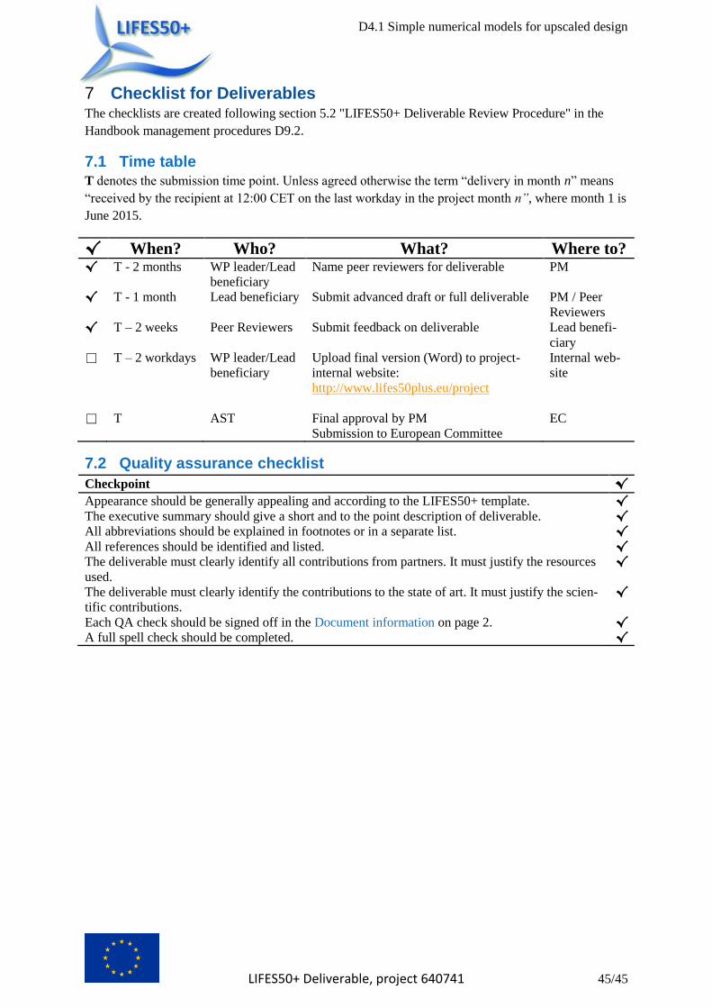
D4.1 Simple numerical models for upscaled design
LIFES50+ Deliverable, project 640741 45/45
Checklist for Deliverables 7The checklists are created following section 5.2 "LIFES50+ Deliverable Review Procedure" in the
Handbook management procedures D9.2.
7.1 Time table
T denotes the submission time point. Unless agreed otherwise the term “delivery in month n” means
“received by the recipient at 12:00 CET on the last workday in the project month n”, where month 1 is
June 2015.
√ When? Who? What? Where to? √ T - 2 months WP leader/Lead
beneficiary
Name peer reviewers for deliverable PM
√ T - 1 month Lead beneficiary
Submit advanced draft or full deliverable PM / Peer
Reviewers √ T – 2 weeks Peer Reviewers Submit feedback on deliverable Lead benefi-
ciary
☐ T – 2 workdays WP leader/Lead
beneficiary
Upload final version (Word) to project-
internal website:
http://www.lifes50plus.eu/project
Internal web-
site
☐ T AST Final approval by PM
Submission to European Committee
EC
7.2 Quality assurance checklist
Checkpoint √
Appearance should be generally appealing and according to the LIFES50+ template. √
The executive summary should give a short and to the point description of deliverable. √
All abbreviations should be explained in footnotes or in a separate list. √
All references should be identified and listed. √
The deliverable must clearly identify all contributions from partners. It must justify the resources
used.
√
The deliverable must clearly identify the contributions to the state of art. It must justify the scien-
tific contributions.
√
Each QA check should be signed off in the Document information on page 2. √
A full spell check should be completed. √
Top Related