


Languages
Pages
Legal

QE Auctions of Treasury Bonds∗
Zhaogang Song† Haoxiang Zhu‡
July 28, 2016
Abstract
The Federal Reserve (Fed) uses auctions to implement its quantitative-easing purchases
of Treasury bonds. To evaluate dealers’ offers on multiple bonds, the Fed relies on its
internal yield-curve model, fitted to secondary market bond prices. Using a proprietary
dataset of QE auctions from November 2010 to September 2011, we find that the Fed
pays 0.71–2.73 cents per $100 par value above the secondary market ask prices. A one-
standard-deviation increase in bond “cheapness”—how much the bond market price
is below a yield-curve-model-implied value—increases auction costs by 6.3 cents per
$100 par value, controlling for standard covariates. We further document great hetero-
geneity of profit margins across dealers with comparable sale amounts, and link this
heterogeneity to cheapness. Our results are consistent with dealers’ strategic bidding
behaviors based on their information about the Fed’s relative valuations of multiple
bonds.
Key Words: Auction, Federal Reserve, Quantitative Easing, Treasury Bond
JEL classification: G12, G13
∗For helpful discussions and comments, we thank Tobias Adrian, Jeremy Bulow, Hui Chen, Jim Clouse,Stefania D’Amico, Darrell Duffie, Michael Fleming, Glenn Haberbush, Jennifer Huang, Jeff Huther, RonKaniel, Leonid Kogan, Arvind Krishnamurthy, Haitao Li, Debbie Lucas, Laurel Madar, Andrey Malenko,Martin Oehmke, Jun Pan, Jonathan Parker, Tanya Perkins, Monika Piazzesi, Simon Potter, Tony Rodrigues,Ken Singleton, Adrien Verdelhan, Jiang Wang, Min Wei, Wei Xiong, Amir Yaron, Rob Zambarano, andHao Zhou as well as seminar participants at the 2014 NBER Summer Institute (Asset Pricing), the ThirdInternational Conference on Sovereign Bond Markets (NYU Stern), CKGSB, Tsinghua PBC, and MIT. Thispaper was written while Zhaogang Song was at the Board of Governors of the Federal Reserve System.†Carey Business School, Johns Hopkins University, 100 International Drive, Baltimore, MD 21202. E-
mail: [email protected].‡MIT Sloan School of Management and NBER, 100 Main Street E62-623, Cambridge, MA 02142.

QE Auctions of Treasury Bonds
July 28, 2016
Abstract
The Federal Reserve (Fed) uses auctions to implement its quantitative-easing purchases of
Treasury bonds. To evaluate dealers’ offers on multiple bonds, the Fed relies on its internal
yield-curve model, fitted to secondary market bond prices. Using a proprietary dataset of
QE auctions from November 2010 to September 2011, we find that the Fed pays 0.71–2.73
cents per $100 par value above the secondary market ask prices. A one-standard-deviation
increase in bond “cheapness”—how much the bond market price is below a yield-curve-
model-implied value—increases auction costs by 6.3 cents per $100 par value, controlling
for standard covariates. We further document great heterogeneity of profit margins across
dealers with comparable sale amounts, and link this heterogeneity to cheapness. Our results
are consistent with dealers’ strategic bidding behaviors based on their information about the
Fed’s relative valuations of multiple bonds.
1 Introduction
One of the most significant events in the history of the U.S. Treasury market is the Federal
Reserve (Fed)’s large-scale asset purchase programs of long-term Treasury securities since the
2008 financial crisis, commonly known as “quantitative easing” (QE).1 Up to September 2011,
the end of the sample period in our study, the Fed purchased $1.19 trillion of Treasury bonds,2
equivalent to about 28% of the total outstanding stock of these securities at the beginning
of the QE program of Treasury securities in March 2009. Given their sheer scale, these
purchase operations must be conducted in a manner that encourages competitive pricing to
avoid excessive execution costs and undesirable burdens on U.S. taxpayers (Potter (2013)).
To purchase such huge amounts of Treasury bonds in a relatively short time window, the
Fed used an auction mechanism that involves buying multiple bonds (CUSIPs) in a single
auction. In this paper, we quantify the costs of QE auctions and investigate their economic
determinants. The unique feature of QE auctions is that the Fed evaluates offers on multiple
bonds using its internal yield curve model and secondary market bond prices (Sack (2011)).
We provide substantive evidence that the Fed’s costs in QE auctions are increasing in bond
“cheapness”—how much the bond market price is below a yield-curve-model-implied value.
Our results are consistent with dealers’ strategic bidding behaviors based on their information
about the Fed’s relative valuations of multiple bonds.
QE auctions are organized as a series of multi-object, multi-unit, and discriminatory-
price auctions, implemented by the Federal Reserve Bank of New York. The only direct
participants are primary dealers recognized by the Fed. For each purchase operation, the
Fed announces a range of total amount and a maturity bucket of the Treasury bonds to be
purchased, but specifies neither the exact total amount nor the amount for individual bonds.
Multiple offers, up to nine on each bond, can be submitted across all eligible securities
simultaneously. Holding a single simultaneous auction for multiple CUSIPs offers much
faster execution than holding separate auctions for individual CUSIPs.
To evaluate offers across multiple bonds, the Fed compares the offered prices to its in-
ternal benchmark prices, according to the Federal Reserve Bank of New York. That is, after
adjusting for its internal benchmark prices, the Fed treats different CUSIPs as perfect sub-
stitutes. Moreover, the Fed’s internal benchmark prices are calculated from a confidential
1The large-scale asset purchase programs began with the purchasing of agency mortgage-backed securitiesand agency debt announced in November 2008. Since our study focuses on purchases of Treasury bonds, weshall use QE for purchase operations of Treasury securities throughout the paper.
2In this paper, we use “bonds” to refer to Treasury securities with maturity above one year, withoutdistinguishing “Treasury notes” and “Treasury bonds.”
1
spline model, fitted on the secondary market prices of Treasury securities. Taking market
bond prices into account helps the Fed to identify “undervalued” securities that are particu-
larly suitable for the Fed to hold. On the other hand, although the Fed’s exact yield-fitting
model is confidential, the use of publicly available bond prices as model inputs can make
the Fed’s relative valuations on different bonds partly predictable by the market, especially
the primary dealers, for a few reasons. First, fixed-income investors and dealers routinely
fit yield-curve models to evaluate the cheapness or richness of different bonds; hence, they
have in-depth professional knowledge of these models.3 Second, primary dealers have years
of experience interacting with the Fed through its permanent and temporary open market
operations. Third, it is not uncommon for former Fed employees to work for primary dealers,
after probationary periods.
Our empirical analysis employs a propriety dataset that includes the 139 purchase auc-
tions of nominal Treasury securities from November 12, 2010 to September 9, 2011, with a
total purchased amount of $780 billion in par value. This amount includes the entire pur-
chase of the “QE2” program, $600 billion, as well as the $180 billion reinvestment by the Fed
of the principal payments from its agency debt and agency MBS holdings. The distinguish-
ing feature of our study is the use of detailed data of each accepted offer, including dealers’
identities, released by the Fed in accordance with the Dodd-Frank Wall Street Reform and
Consumer Protection Act (Dodd-Frank Act), passed in July 2010. This allows us to study
not only the auction costs at the aggregate level, but also the granular heterogeneity across
auctions, bonds, and dealers.
We measure the costs to the Fed by the difference between the accepted offer prices
and the secondary market prices, weighted by the accepted quantity. The secondary market
prices are obtained from the Federal Reserve Bank of New York, quoted at 8:40am, 11:30am,
2:15pm, and 3:30pm. The vast majority of QE auctions close at 11am. So for those auctions,
our auction costs measured relative to the closest ask price in the secondary market at
11:30am can be viewed as the “realized costs” of the Fed 30 minutes after the auction, or
interpreted as the profit of dealers in selling bonds to the Fed at 11am and then covering
their short positions in the secondary markets 30 minutes later (see Hasbrouck (2007) for a
discussion of realized cost). We also use the secondary market prices at 2:15pm and 3:30pm
to compute auction costs. On average, the Fed pays 0.71 cents per $100 par value above
secondary market ask prices near the close of the auction, 2.73 cents above the 2:15pm
3See Duarte, Longstaff, and Yu (2007) for studies of the yield curve arbitrage strategy of fixed-incomehedge funds.
2
secondary market ask prices, and 2.15 cents above the 3:30pm secondary market ask prices.
The auction price markups also vary substantially across the 139 QE auctions, with a
standard deviation of 10-20 cents per $100 par value. A natural question is what drives the
time variation in auction costs. Recall that the unique feature of QE auctions is that the
Fed values the offers across bonds based on internal benchmark prices, which we conjecture
are partly predictable by the market. Although we do not observe the Fed’s model, we
construct a bond cheapness measure using standard techniques. To the extent that the
actual model and data used by the Fed and the dealers are strictly more accurate, our
estimated effect of bond cheapness on auction costs would be conservative. Specifically, we
first fit a Svensson (1994) yield curve model at the beginning of each auction day. Then,
for each CUSIP, we measure its cheapness by the difference between the fitted-yield-curve-
implied price and the secondary market ask price, in cents per $100 par value. Our fitted
yield curve is highly correlated with the popular “GSW” (Gurkaynak, Sack, and Wright
(2007)) yield curve maintained by the Fed.4
Besides cheapness, we also take into account two standard economic channels of price
markup. One is bond value uncertainty, measured by the volatility of bond returns during
the five days before the auction date. Models of common value auctions (e.g., Wilson (1968)
and Ausubel, Cramton, Pycia, Rostek, and Weretka (2013)) suggest that a higher value
uncertainty increases auction price markup. In addition, we consider a few measures of bond
illiquidity and scarcity, including the specialness (how costly it is to borrow a particular bond
in the repo market), the bid-ask spread, and the outstanding balance of a particular bond.
We expect the auction cost to be higher if the bond is more special or is less liquid.
We run panel regressions of the auction price markup across bonds and auctions on bond
cheapness, as well as volatility, specialness, bid-ask spread, and outstanding balance, con-
trolling for CUSIP fixed effects and expected auction sizes. We find that a higher cheapness
is associated with a higher auction price markup. A one standard deviation increase in the
cheapness measure (across auctions and CUSIPs) increases the bond price markup by 6.3
cents per $100 par value. The auction price markup also has significant positive loadings on
volatility and specialness, implying that both the winner’s curse and scarcity increase the
auction cost. A one standard deviation increase in volatility and specialness increases bond
price markup by 3.8 cents and 2.1 cents, respectively (again per $100 par value).
Our main results on the determinants of auction costs are robust to the exact time
at which the costs are measured, the universe of bonds included in the yield-curve-fitting
4See http://www.federalreserve.gov/pubs/feds/2006/200628/200628abs.html.
3
model, the yield-curve-fitting model itself, and time-series controls such as yield and yield
volatilities, demonstrated in a series of robustness checks.
Because the cost to the Federal Reserve is the profit of primary dealers, we characterize
dealers’ profitability next. Taking advantage of dealer identities in our proprietary dataset,
we reveal the granular heterogeneity of profitability across primary dealers in participating
in QE auctions. We measure a dealer’s profit margin as the prices of accepted offers less
the secondary market prices closest to the auction time, weighted by accepted quantities.
Among the 20 primary dealers that participated in QE auctions, the top five have large
sale amounts and high profit margins (1.67 cents per $100 par value on average), while the
bottom few dealers sell similarly large amounts but receive negative profit margins (−0.44
cents per $100 par value on average).
Given the importance of bond cheapness in determining auction costs, we naturally con-
jecture that the heterogeneity in dealers’ profit margin is driven, at least partly, by the
heterogeneity in their ability to sell bonds that are deemed cheaper by the Fed. For in-
stance, it would be the case if some dealers had better information of the Fed’s yield curve
model. Alternatively, some dealers may simply be better at finding those bonds. To inves-
tigate the source of the heterogeneity in dealers’ profit margin, we run panel regressions of
profit margins on cheapness, volatility, and specialness, measured for each winning dealer in
each auction. Consistent with the above conjecture, we find that a dealer’s profit margin
has a significant and positive loading on bond cheapness. A one standard deviation increase
in a bond’s cheapness (across auction and dealer) increases the auction price markup by 3.8
cents per $100 par value. Dealers’ profit margins also have a positive and significant loading
on specialness, and a negative and significant loading on outstanding balance. Together,
this evidence suggests that dealers who make more money do so by selling bonds that are
deemed cheaper by the Fed or are more costly to locate or finance (more special and lower
outstanding balance).
We caution that our results do not make any policy prescription on the optimal repurchase
mechanism. The Fed pays a higher cost on bonds that appear cheaper relative to model-
implied bond prices, but it is precisely on those “undervalued” bonds that the gains from
trade between the Fed and the market are likely the largest. Moreover, as we discuss later,
the auction costs seem modest in comparison with Treasury issuance auctions, suggesting
that auction is a reasonable, if not perfect, mechanism for implementing quantitative easing.
To the best of our knowledge, this paper provides the first empirical analysis of the im-
plementation mechanism of quantitative easing, hence complementing a large literature on
4
the effect of quantitative easing on interest rates (see Krishnamurthy and Vissing-Jorgensen
(2011), Gagnon, Raskin, Remanche, and Sack (2011), Hancock and Passmore (2011), Swan-
son (2011), Wright (2012), D’Amico, English, Lopez-Salido, and Nelson (2012), Hamilton
and Wu (2012), Christensen and Rudebusch (2012), Stroebel and Taylor (2012), Bauer and
Rudebusch (2013), Li and Wei (2013), D’Amico and King (2013), Meaning and Zhu (2011),
and Eser and Schwaab (2016), among others).
The paper most closely related to our work is Han, Longstaff, and Merrill (2007), who
analyze the Treasury’s buyback auctions of long-term securities from March 2000 to April
2002. Our study of QE auctions differs in at least two important aspects. First, though
both are discriminatory-price auctions and involve different CUSIPs, QE auctions have an
explicitly announced mechanism, whereas the mechanism of the Treasury’s buyback auctions
is opaque. We argue that the transparency of the QE auction mechanism is partly why the
Fed’s preference becomes predictable, which is, in turn, linked to auction costs. Second, our
data include individual accepted offers and dealer identities on each CUSIP in each auction,
which are more comprehensive than the CUSIP-level aggregate auction data used by Han,
Longstaff, and Merrill (2007). Dealer-level data enable us to look into the heterogeneity of
dealers and link it to the Fed’s relative valuation, a unique economic channel of QE auctions.
More recently, Pasquariello, Roush, and Vega (2014) study how the Fed’s open mar-
ket operations in normal times affect the Treasury market microstructure, using only the
purchase amount. We differ by focusing on the auction implementation of unconventional
monetary policy, and by using detailed offer-level data of primary dealers.
Our paper is also related to the large literature on Treasury issuance auctions, such as
Cammack (1991), Simon (1994), and Nyborg and Sundaresan (1996), who use aggregate
auction-level data, and Umlauf (1993), Gordy (1999), Nyborg, Rydqvist, and Sundaresan
(2002), Keloharju, Nyborg, and Rydqvist (2005), Hortacsu and McAdams (2010), Kastl
(2011), and Hortacsu and Kastl (2012), who use bid-level data.5 QE auctions differ in that
each auction involves multiple substitutable CUSIPs, whereas each issuance auction has
one CUSIP at a time. We show how the market seems to take advantage of the relative
valuations of multiple CUSIPs by the Fed. Moreover, prior studies of issuance auctions
either do not have dealer identities or only have masked identifiers, whereas our data include
dealer identities on each CUSIP in each auction, allowing us to study the heterogeneity of
dealers’ profitability.
5Theoretical and experimental studies of Treasury issuance auctions include Bikhchandani and Huang(1989), Chatterjee and Jarrow (1998), Goswami, Noe, and Rebello (1996), and Kremer and Nyborg (2004),among others.
5

2 Institutional Background of QE Auctions
From November 12, 2010 to September 9, 2011, the Federal Reserve conducted a series of 156
purchase auctions of U.S. Treasury securities, including Treasury notes, bonds, and Inflation-
Protected Securities. (We discuss our data and choice of sample period in Section 4.) These
auctions cover two Fed programs. The first, commonly referred to as QE2, is the $600 billion
purchase program of Treasury securities, announced on November 3, 2010 and finished on
July 11, 2011. The second program is the reinvestment of principal payments from agency
debt and agency MBS into longer-term Treasury securities, announced on August 10, 2010,
with a total purchase size of $180 billion over our sample period.6 These actions are expected
to maintain downward pressure on longer-term interest rates, support mortgage markets,
and help to make broader financial conditions more accommodative, as communicated by
the Federal Open Market Committee (FOMC).
QE auctions are designed as a series of sealed-offer, multi-object, multi-unit, and discriminatory-
price auctions. Transactions are conducted on the FedTrade platform. Direct participants
of QE auctions only include the primary dealers recognized by the Federal Reserve Bank of
New York, although other investors can indirectly participate through the primary dealers.7
Figure 1 describes the timeline of a typical QE auction, including pre-auction announce-
ment, auction execution, and post-auction information release. To initiate the asset purchase
operation, the Fed makes a pre-auction announcement on or around the eighth business day
of each month. The announcement includes an anticipated total amount of purchases ex-
pected to take place between the middle of the current month and the middle of the following
month.8 Most importantly, this announcement also includes a schedule of anticipated Trea-
6Principal payments from maturing Treasury securities are also invested into purchases of Treasury secu-rities in auctions.
7In the first half of our sample period until February, 2, 2011, there were 18 primary dealers, includingBNP Paribas Securities Corp (BNP Paribas), Bank of America Securities LLC (BOA), Barclays Capital Inc(Barclays Capital), Cantor Fitzgerald & Co (Cantor Fitzgerald), Citigroup Global Markets Inc (Citigroup),Credit Suisse Securities USA LLC (Credit Suisse), Daiwa Securities America Inc (Daiwa), Deutsche BankSecurities Inc (Deutsche Bank), Goldman Sachs & Co (Goldman Sachs), HSBC Securities USA Inc (HSBC),Jefferies & Company, Inc (Jefferies), J. P. Morgan Securities Inc (J. P. Morgan), Mizuho Securities USAInc (Mizuho), Morgan Stanley & Co. Incorporated (Morgan Stanley), Nomura Securities International, Inc(Nomura), RBC Capital Markets Corporation (RBC), RBS Securities Inc (RBS), and UBS Securities LLC(UBS). On February 2, 2011, MF Global Inc (MF Global) and SG Americas Securities, LLC (SG Americas)were added to the list of primary dealers, making the total number of primary dealers 20 in the second halfour sample period. See the website of the Federal Reserve Bank of New York for the historical list of primarydealers.
8This amount is determined by the part of the $600 billion purchases that are planned to be completedover the coming monthly period, and the sum of the approximate amount of principal payments from agencyMBS expected to be received over the monthly period, and the amount of agency debt maturing between
6

Figure 1: Example of Timeline of QE Auctions
sury purchase operations, including operation dates, settlement dates, security types to be
purchased (nominal coupons or TIPS), the maturity date range of eligible issues, and an
expected range for the size of each operation. Therefore, the announcement identified the
set of eligible bonds to be included as well as the minimum and maximum total par amount
(across all bonds) to be purchased in each planned auction. While the purchase amount has
to reach the minimum expected size, the Fed reserves the option to purchase less than the
maximum expected size.
On the auction date, each dealer submits up to nine offers per security or CUSIP, with
both the minimum offer size and the minimum increment as $1 million. Each offer consists
of a price-quantity pair, specifying the par value the dealer is willing to sell to the Fed at
a specific price. The auctions happen mostly between 10:15am to 11:00am Eastern Time.
Very rarely, the auctions happen between 10:40am and 11:30am, 11:25am and 12:05pm, and
1:15pm and 2:00pm. Out of the 139 auctions we analyze, one is closed at 11:30am, one is
closed at 12:05pm, and three are closed at 2pm. The rest 134 auctions are all closed at
the seventh business day of the current month and the sixth business day of the following month. All thepurchases are conducted as one consolidated purchase program.
7
11:00am.
Within a few minutes after the closing of the auction, the Fed publishes the auction
results on the Federal Reserve Bank of New York website, including the total number of
offers received, total number of offers accepted, and the amount purchased per CUSIP. At
the same time, participating dealers receive their accepted offers via FedTrade. At the end of
each scheduled monthly period, coinciding with the release of the next period’s schedule, the
Fed publishes certain auction pricing information. The pricing information released includes
the weighted-average accepted price, the highest accepted price, and the proportion accepted
of each offer submitted at the highest accepted price, for each security purchased in each
auction. Finally, in accordance with the Dodd-Frank Act, detailed auction results including
the offer price, quantity, and dealer identity for each accepted individual offer will be released
two years after each quarterly auction period.
In a discriminatory-price auction, offers are either accepted or rejected at the specified
prices, and for each accepted offer, the dealer sells its offering amount of bonds to the Fed
at the offered price. Since each auction involves a set of heterogeneous securities/CUSIPs,
an algorithm is needed to rank offers on different CUSIPs. To make this ranking, the Fed
compares each offer with a benchmark price of the bond for that offer calculated from its
internal spline-based yield curve model fitted to the secondary market prices of Treasury
securities (Sack (2011)). Thus, these spline-based benchmark prices make different CUSIPs
perfect substitutes from the Fed’s perspective.
Conditional on filling the desired par purchase amount, the Fed would naturally prefer
bonds that trade at a discount in the secondary market relative to otherwise similar bonds.
This way, the Fed behaves like a long-term buy-and-hold investor. Although the Fed does
not publish its spline yield curve model or estimated benchmark prices, we expect sophis-
ticated investors and primary dealers to have some information about the Fed’s yield curve
algorithm. After all, fitting yield-curve models is a route practice by sophisticated fixed-
income investors and dealers for evaluating the relative cheapness or richness of different
bonds. Moreover, dealers may gain information about the Fed’s relative valuations through
years of interaction and by hiring former Fed employees. As we see in the standard auction
model of the next section, if dealers have information about the Fed’s relative valuations,
bonds that appear cheaper to the Fed will incur a higher cost.
8
3 Implications of Auction Theory for QE Auctions
QE auctions are multiple-object, multiple-unit and discriminatory-price auctions. To the
best of our knowledge, this unique combination of institutional features is not yet addressed
in existing auction models. In fact, even for a single-object, multiple-unit auction, multiple
Bayesian-Nash equilibria can exist, so that no definitive theoretical predictions can be made
about the equilibrium bidding strategies and auction outcomes (see, for example, Bikhchan-
dani and Huang (1993); Back and Zender (1993); Ausubel, Cramton, Pycia, Rostek, and
Weretka (2013)). The complications of multiple objects and internal spline-based prices in-
volved in QE auctions make a thorough theoretical treatment of QE auctions much more
challenging.
Instead of pursuing a full-fledged theory, which is beyond the empirical focus of this
paper, we use the standard theory of single-unit auctions to illustrate how dealers’ infor-
mation about the Fed’s yield curve model affects the auction price markup and guide our
empirical analysis. Similar approach is employed in empirical studies of Treasury issuance
auctions, such as Cammack (1991), Umlauf (1993), Gordy (1999), and Keloharju, Nyborg,
and Rydqvist (2005).
Suppose there are N dealers participating in QE auctions. Consider a bond to be pur-
chased by the Fed in QE auctions. Denote dealer i’s valuation of the bond by vi. In general,
there are two components in vi: (i) the common value component that captures the resale
value of the bond in the secondary market; and (ii) the private value component that cap-
tures a dealer’s idiosyncratic cost in obtaining the bond or private information about the
bond. In practice, the common-value component is reflected (at least partly) in the secondary
market quotes on various electronic trading platforms available to market participants, such
as Bloomberg, BrokerTec, eSpeed, and TradeWeb. The private-value component is affected
by a dealer’s existing inventory, the cost of financing the bonds in the repo markets, and his
relationship with customers and other dealers.
One classical implication from the common-value component is the winner’s curse prob-
lem: because no dealer is absolutely certain about the resale value of a bond, a dealer worries
about buying the bonds too expensively or selling it too cheaply. Applied to QE auctions, a
more severe winner’s curse problem implies that dealers will submit higher offers to the Fed,
leading to a higher expected cost of the Fed. For simplicity, we will not formally reproduce
this standard argument here (see Cammack (1991), Umlauf (1993), Keloharju, Nyborg, and
Rydqvist (2005), and Han, Longstaff, and Merrill (2007) for more discussions). But the win-
ner’s curse channel predicts that a higher bond value uncertainty leads to a higher expected
9
cost of the Fed in QE auctions.
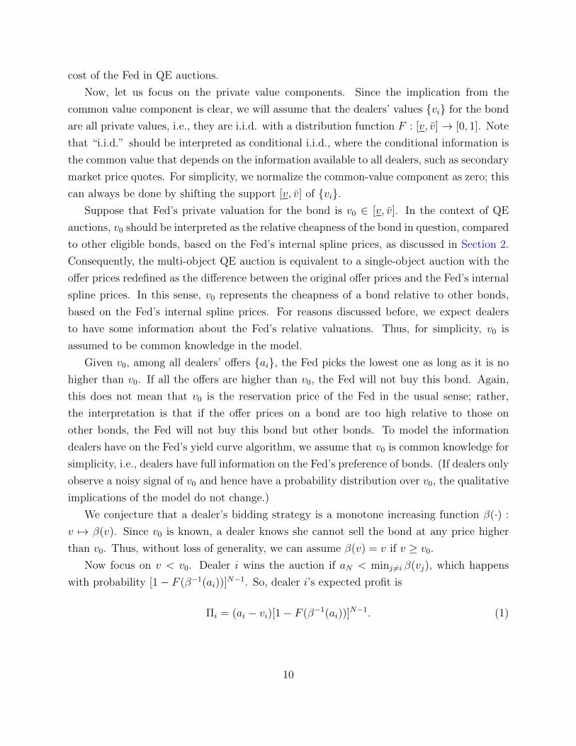
Now, let us focus on the private value components. Since the implication from the
common value component is clear, we will assume that the dealers’ values {vi} for the bond
are all private values, i.e., they are i.i.d. with a distribution function F : [v, v̄]→ [0, 1]. Note
that “i.i.d.” should be interpreted as conditional i.i.d., where the conditional information is
the common value that depends on the information available to all dealers, such as secondary
market price quotes. For simplicity, we normalize the common-value component as zero; this
can always be done by shifting the support [v, v̄] of {vi}.Suppose that Fed’s private valuation for the bond is v0 ∈ [v, v̄]. In the context of QE
auctions, v0 should be interpreted as the relative cheapness of the bond in question, compared
to other eligible bonds, based on the Fed’s internal spline prices, as discussed in Section 2.
Consequently, the multi-object QE auction is equivalent to a single-object auction with the
offer prices redefined as the difference between the original offer prices and the Fed’s internal
spline prices. In this sense, v0 represents the cheapness of a bond relative to other bonds,
based on the Fed’s internal spline prices. For reasons discussed before, we expect dealers
to have some information about the Fed’s relative valuations. Thus, for simplicity, v0 is
assumed to be common knowledge in the model.
Given v0, among all dealers’ offers {ai}, the Fed picks the lowest one as long as it is no
higher than v0. If all the offers are higher than v0, the Fed will not buy this bond. Again,
this does not mean that v0 is the reservation price of the Fed in the usual sense; rather,
the interpretation is that if the offer prices on a bond are too high relative to those on
other bonds, the Fed will not buy this bond but other bonds. To model the information
dealers have on the Fed’s yield curve algorithm, we assume that v0 is common knowledge for
simplicity, i.e., dealers have full information on the Fed’s preference of bonds. (If dealers only
observe a noisy signal of v0 and hence have a probability distribution over v0, the qualitative
implications of the model do not change.)
We conjecture that a dealer’s bidding strategy is a monotone increasing function β(·) :
v 7→ β(v). Since v0 is known, a dealer knows she cannot sell the bond at any price higher
than v0. Thus, without loss of generality, we can assume β(v) = v if v ≥ v0.
Now focus on v < v0. Dealer i wins the auction if aN < minj 6=i β(vj), which happens
with probability [1− F (β−1(ai))]N−1. So, dealer i’s expected profit is
Πi = (ai − vi)[1− F (β−1(ai))]N−1. (1)
10

By the standard first-order condition, we can solve
β(v) = v +
∫ v0u=v
(1− F (u))N−1du
(1− F (v))N−1, v ∈ [v, v0]. (2)
Under this strategy, if the Fed accepts the best offer, the Fed’s cost is mini β(vi). Thus, a
higher offer β(·) implies a higher expected cost to the Fed.
All else equal, β(v) is increasing in v0 for v ∈ [v, v0], for all finite N . This predicts that
the auction price is higher if the Fed’s value v0 of the bond is higher. Intuitively, this is
because dealers have market power and behave strategically, which is standard in auction
theory. Given the interpretation of v0 as the relative bond cheapness, this implies that the
auction price is higher if the bond looks “cheaper” based on the Fed’s spline-implied bond
value.
In the subsequent empirical analysis, we will construct a measure of bond “cheapness”
to proxy for the dealers’ information about the Fed’s value v0. We will also control for the
standard winner’s curse problem by using a proxy for bond value uncertainty.
4 Data and Summary Statistics
In this section, we describe the data and basic summary statistics of the outcomes of QE
auctions. Summary statistics include the characteristics of bonds covered in QE auctions,
auction size, number of winning offers, and number of winning dealers.
4.1 Data
Our sample period is from November 12, 2010 to September 9, 2011. We focus on this sample
period mainly because this is the only QE period during which the Fed purchased only
Treasury securities and for which the detailed data of dealer offers are available. Specifically,
the Dodd-Frank Act, passed on July 21, 2010 by the U.S. Congress, mandates that the
Federal Reserve should release detailed auction data to the public with a two-year delay
after each quarterly operation period. In consequence, detailed dealer offers are available
from July 22, 2010. We discard the period July 22, 2010–November 11, 2010 because no
orderly expected purchase sizes at the auction level were announced by the Fed in this period.
Moreover, on September 21, 2011, the Fed announced the Maturity Extension Program and
changes in the agency debt and agency MBS reinvestment policy, which lead to purchases
11
of agency MBS and sales of short-term Treasury securities in addition to purchases of long-
term Treasury securities thereafter. Therefore, to avoid potential compounding effects due
to other policy operations, we discard the period starting from September 21, 2011 to focus
on a “clean” period of only Treasury bond purchases, In addition, we discard the period
September 10, 2011–September 20, 2011 because the monthly planned operation of this
September is interrupted by the policy change on September 21, 2011.
We focus on 139 auctions of nominal Treasury securities among the 156 purchase auctions
between November 12, 2010 and September 9, 2011. The excluded 17 auctions of TIPS only
account for 3% of the total purchases in terms of par value. Moreover, focusing on auctions of
nominal bonds makes the bond characteristics, such as coupon rates and returns, comparable
across CUSIPs. These 139 auctions were conducted on 136 days, with two auctions on each
of November 29, 2010, December 20, 2010, and June 20, 2011, and only one auction on all
the other days.
Our empirical analysis combines the auction data released by the Federal Reserve and
three CUSIP-level datasets of Treasury securities, including the secondary market intraday
price quotes, the specific collateral repo rates, and the outstanding quantity. The auction
data include: (1) the expected total purchase size range, the total par value offered, and the
total par value accepted for each auction; (2) the indicator of whether a CUSIP was included
or excluded in the auctions; (3) for bonds included in the auctions, the par value accepted,
the weighted average accepted price, and the least favorable accepted price for each CUSIP
in each auction; and (4) the offered par value, offer (clean) price, and dealer identity for each
accepted offer on each CUSIP in each auction.
To the best of our knowledge, the individual-offer data we use is the first set of auction
data at the individual bid level that has been ever analyzed for U.S. Treasury securities. Pre-
vious studies of issuance auctions and buyback auctions of U.S. Treasury securities, including
Cammack (1991), Simon (1994), Nyborg and Sundaresan (1996), and Han, Longstaff, and
Merrill (2007), have used data only at the aggregate auction level or at the CUSIP level at
best.9
Our secondary market price data contain indicative bid and ask quotes from the New
Price Quote System (NPQS) by the Federal Reserve Bank of New York, as well as the
corresponding coupon rate, original maturity at issuance, and remaining maturity, which
are also used by D’Amico and King (2013). There are four pairs of bid and ask quotes each
9Studies of Treasury auctions in other countries have used bid-level data, such as Umlauf (1993), Gordy(1999), Nyborg, Rydqvist, and Sundaresan (2002), Keloharju, Nyborg, and Rydqvist (2005), Hortacsu andMcAdams (2010), Kastl (2011), and Hortacsu and Kastl (2012).
12
day, which are the best bid and ask prices across different trading platforms of Treasury
securities made at 8:40am, 11:30am, 2:15pm, and 3:30pm. We choose these NPQS quotes
because the these data cover off-the-run securities that are targeted in QE auctions. (By
contrast, the BrokerTec data used in recent studies such as Fleming and Mizrach (2009) and
Engle, Fleming, Ghysels, and Nguyen (2012) mainly contain prices of newly issued on-the-
run securities.) Moreover, these price quotes are important sources for the Fed’s internal
spline algorithm and benchmark prices. Hence, our bond cheapness measure using NPQS
prices as inputs is probably correlated with the Fed’s true preference. Strictly speaking, it
would be even better to have higher-frequency price quotes throughout the day, but such
data are unavailable to us.
We obtain the CUSIP-level special collateral repo rates from the BrokerTec Interdealer
Market Data that averages quoted repo rates across different platforms between 7am and
10am each day (when most of the repo trades take place). We then calculate the CUSIP-level
repo specialness as the difference between the General Collateral (GC) repo rate and specific
collateral repo rate, measured in percentage points. This specialness measure reflects the
value of a specific Treasury security used as a collateral for borrowing (see Duffie (1996);
Jordan and Jordan (1997); Krishnamurthy (2002); Vayanos and Weill (2008); D’Amico, Fan,
and Kitsul (2013)). We also obtain the outstanding par value of Treasury securities each
day from the Monthly Statement of the Public Debt (MSPD) of the Treasury Department.
4.2 Summary Statistics: Bonds Covered in QE Auctions
What Treasury securities does the Fed buy and what is the allocation of purchasing quantities
across different securities? Table 1 reports the maturity distribution of planned purchases in
QE Auctions of Treasury debt over our sample period, announced on November 3, 2010 by
the Fed. Only 6% of planned purchase amounts have a maturity beyond 10 years. According
to the Fed, this maturity distribution has an average duration of between 5 and 6 years for
the securities purchased. The Fed does not purchase Treasury bills, STRIPS, or securities
traded in the when-issued market.10
Panel A of Table 2 presents descriptive statistics on the number of bonds for the 139
QE auctions (of nominal Treasury securities) in our sample period. The number of eligible
bonds in an auction varies between 15 and 36, with a mean of 26. On average, one CUSIP
is excluded in each auction, with the minimum and maximum number of excluded CUSIPs
being 0 and 4, respectively. This leaves the number of eligible (included) bonds between
10See http://www.newyorkfed.org/markets/lttreas_faq_101103.html for details.
13

Table 1: Maturity Distribution of Planned Purchases in QE Auctions
Maturity Sectors for QE Auctions of Treasury Securities
Nominal Coupon Securities TIPS
Maturity Sector (Years) 1.5–2.5 2.5–4 4–5.5 5.5–7 7–10 10–17 17–30 1.5–30
Percentage 5% 20% 20% 23% 23% 2% 4% 3%
Note: This table shows the maturity distribution of planned purchases in QE Auctions of Treasury debt over
our sample period (November 12, 2010–September 9, 2011), announced on November 3, 2010 by the Fed.
The on-the-run 7-year note will be considered part of the 5.5- to 7-year sector, and the on-the-run 10-year
note will be considered part of the 7- to 10-year sector.
13 and 34, averaging 25 per auction. Among these included bonds, in each auction the Fed
purchases between 2 and 26 bonds, with an average of 14 bonds. On average, in each auction,
11 eligible bonds are not purchased by the Fed. Across all 139 auctions, only 186 CUSIPs
have ever been purchased by the Fed, among the 215 eligible CUSIPs.
According to the Fed’s communications to the public, excluded bonds are those trading
with heightened specialness in the repo market, or the cheapest to deliver into the front-
month Treasury futures contracts.11 Presumably, these bonds are excluded to avoid creating
or exacerbating supply shortages in repo and futures markets.
To formally explore the Fed’s decision to include or exclude certain CUSIPs, we estimate
a panel logit regression as follows:
ln[Itj/(1− Itj)] =∑t
αtDt + β1 · Specialensstj + β2 ·Maturitytj + β3 · CPj + εit, (3)
where Itj is the probability of bond j being included in the t-th auction, Maturitytj is
the time to maturity measured in years, and CPj is the coupon rate in percentage points.
Because our objective here is to check what type of bonds the Fed includes in an auction,
we include auction fixed effects Dt.
Panel B of Table 2 reports the results from the panel Logit regression (3), as well as
regressions with only one of Specialensstj, Maturitytj, and CPj on the right-hand side. We
11The Fed also excludes CUSIPs by the size limit for purchase amount per security according to thepercentage of the outstanding issuance and the Fed’s existing holdings of this security. See the websiteof Federal Reserve Bank of New York for details (http://www.newyorkfed.org/markets/lttreas_faq_101103.html). We do not study this criterion as the Fed purchase rarely hit the size limit in our sample.In addition, communications with the Fed confirm that primary dealers have almost perfect foresight aboutwhich securities will be excluded before the auction.
14

Table 2: Summary Statistics of Bonds in QE Auctions
A: Number of Bonds in QE Auctions
Eligible Bonds Excluded Bonds Included Bonds Included Bonds Included Bonds
(not purchased) (purchased)
Mean 26 1 25 11 15
Std 6 1 6 7 5
Min 15 0 13 0 3
Q-25% 20 1 19 5 12
Q-50% 27 1 26 9 15
Q-75% 31 2 29 16 19
Max 36 4 34 28 27
B: Regression of Inclusion Dummy
Maturity -0.078** -0.066**
(-3.445) (-2.837)
CP 0.072 0.072
(1.374) (1.393)
Specialness -7.376** -7.639*
(-2.683) (-2.554)
N 3,127 3,127 3,127 3,127
R2 0.030 0.030 0.054 0.058
Auction FE Yes Yes Yes Yes
Note: Panel A of this table presents descriptive statistics, including mean, standard deviation (std), minimum
(min), maximum (max), and quartiles of the number of bonds covered in the 139 QE auctions of nominal
Treasury securities, from November 12, 2010 to September 9, 2011. Panel B reports panel Logit regressions
of whether a bond is included in an auction (yes=1, no=0), with z-statistics in the parentheses. The auction
fixed effects are included. The right-hand variables are Specialness of a bond (the general repo rate minus
special repo rate on the bond) in percentage points, the coupon rate CP in percentage points, and the
Maturity in years. Significance levels: ∗∗ for p < 0.01, ∗ for p < 0.05, and + for p < 0.1, where p is the
p-value.
observe that the regression coefficient of Specialness is significantly negative, confirming that
the Fed did exclude bonds trading at heightened specialness. Moreover, the Fed also tends
to exclude bonds with longer maturity on average, which is intuitive because, for a fixed
auction and hence a maturity bucket, longer-maturity bonds tend to be closer to on-the-run.
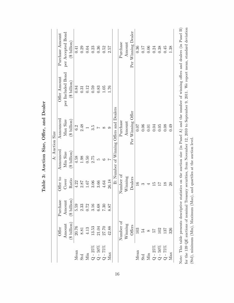
4.3 Summary Statistics: Auction Size, Offer, and Dealer
In this section, we present summary statistics of the auction size, number of winning offers,
and number winning dealers. Panel A of Table 3 shows that the par amounts of submitted
15
Tab
le3:
Auct
ion
Siz
e,
Off
er,
and
Deale
r
A:
Au
ctio
nS
ize
Off
erP
urc
hase
Off
erto
An
nou
nce
dA
nn
oun
ced
Off
erA
mou
nt
Pu
rch
ase
Am
ount
Am
ount
Am
ou
nt
Cov
erM
inS
ize
Max
Siz
ep
erIn
clu
ded
Bon
dp
erA
ccep
ted
Bon
d
($b
illi
on
)($
bil
lion
)R
atio
($b
illi
on)
($b
illi
on)
($b
illi
on)
($b
illi
on)
Mea
n20.7
65.5
94.
224.
586.
20.
840.
41
Std
8.8
12.
332.
871.
982.
480.
310.
29
Min
4.1
30.
721.
670.
501
0.12
0.04
Q-
25%
13.5
33.
163.
062.
753.
50.
590.
23
Q-
50%
21.0
46.
683.
665
70.
830.
36
Q-
75%
27.7
07.
304.
646
81.
050.
52
Max
42.8
88.8
726
.18
79
1.76
2.57
B:
Nu
mb
erof
Win
nin
gO
ffer
san
dD
eale
rs
Nu
mb
erof
Nu
mb
erof
Pu
rchas
eP
urc
has
e
Win
nin
gW
inn
ing
Am
ount
Am
ount
Off
ers
Dea
lers
Per
Win
nin
gO
ffer
Per
Win
nin
gD
eale
r
Mea
n103
160.
070.
36
Std
54
30.
060.
17
Min
84
0.01
0.06
Q-
25%
5715
0.04
0.24
Q-
50%
102
170.
050.
38
Q-
75%
137
180.
080.
45
Max
326
200.
491.
38
Not
e:T
his
tab
lep
rese
nts
des
crip
tive
stat
isti
cson
the
au
ctio
nsi
ze(i
nP
an
elA
)an
dth
enu
mb
erof
win
nin
goff
ers
and
dea
lers
(in
Pan
elB
)
for
the
139
QE
auct
ion
sof
nom
inal
Tre
asu
ryse
curi
ties
,fr
om
Nov
emb
er12,
2010
toS
epte
mb
er9,
2011.
We
rep
ort
mea
n,
stan
dard
dev
iati
on
(Std
),m
inim
um
(Min
),M
axim
um
(Max
),an
dqu
art
iles
at
the
au
ctio
nle
vel.
16

offers vary between $4 and $43 billion, averaging about $21 billion per auction, while the
offer amount accepted by the Fed varies between $0.7 and $8.9 billion, averaging $5.6 billion
per auction. The ratio between submitted and accepted offer amounts (offer-to-cover) is on
average 4.2, with a range of 1.7 to 26.2. The average expected minimum and maximum
auction sizes are $4.6 billion and $6.2 billion, and the accepted offer amount always falls
between the expected minimum and maximum auction sizes. In addition, the offer amount
per included bond is $0.84 billion on average, while the accepted offer amount per accepted
bond is $0.41 billion.
Panel B of Table 3 presents summary statistics on the number of winning offers and
dealers. We observe that the number of winning offers ranges between 8 and 326, with a
mean of 103, whereas the number of winning dealers ranges between 4 and 20, with a mean
of 16. (In our sample period, the total number of primary dealers was 18 before February 2,
2011 and 20 afterwards.) As a result, per auction, each winning offer has an average size of
$0.07 billion, and each winning dealer sells $0.36 billion to the Fed on average.
5 Empirical Results
In this section, we present our empirical findings on the costs of the Federal Reserve in
executing QE auctions and their economic determinants. We first present summary statistics
of the auction costs and then study what economic channels affect auction costs, across bonds
as well as across dealers, using panel regressions.
5.1 How Much Does the Fed Pay?
Following the literature,12 we measure the auction cost as the auction price markup, namely
the difference between the auction price and secondary market price on the days the auctions
are executed.13 Let pt,j,d,o and qt,j,d,o be the o-th winning offer price and par value from dealer
d on CUSIP j in auction t, respectively, and let Pt,j be the secondary market price of the
12See, for example, Han, Longstaff, and Merrill (2007), Cammack (1991), Nyborg and Sundaresan (1996),and Hortacsu and Kastl (2012), among others.
13We also measure the cost of purchasing a bond as the difference between the worst price accepted by theFed (also known as the stop-out price) and the corresponding secondary market price. This cost measurequantifies the maximum price the Fed is willing to tolerate to achieve its minimum purchase amount. Thecost measure based on stop-out price is around 2 cents per $100 par value higher than that based on theweighed average price, and the correlation between the two measures is as high as 99%. Because of theirhigh correlation, we only report results based on the average purchase price.
17
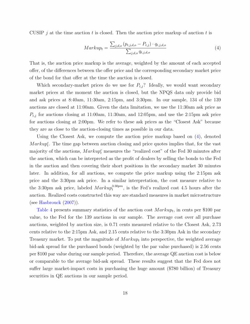
CUSIP j at the time auction t is closed. Then the auction price markup of auction t is
Markupt =
∑j,d,o (pt,j,d,o − Pt,j) · qt,j,d,o∑
j,d,o qt,j,d,o(4)
That is, the auction price markup is the average, weighted by the amount of each accepted
offer, of the differences between the offer price and the corresponding secondary market price
of the bond for that offer at the time the auction is closed.
Which secondary-market prices do we use for Pt,j? Ideally, we would want secondary
market prices at the moment the auction is closed, but the NPQS data only provide bid
and ask prices at 8:40am, 11:30am, 2:15pm, and 3:30pm. In our sample, 134 of the 139
auctions are closed at 11:00am. Given the data limitation, we use the 11:30am ask price as
Pt,j for auctions closing at 11:00am, 11:30am, and 12:05pm, and use the 2:15pm ask price
for auctions closing at 2:00pm. We refer to these ask prices as the “Closest Ask” because
they are as close to the auction-closing times as possible in our data.
Using the Closest Ask, we compute the auction price markup based on (4), denoted
Markupct . The time gap between auction closing and price quotes implies that, for the vast
majority of the auctions, Markupct measures the “realized cost” of the Fed 30 minutes after
the auction, which can be interpreted as the profit of dealers by selling the bonds to the Fed
in the auction and then covering their short positions in the secondary market 30 minutes
later. In addition, for all auctions, we compute the price markup using the 2:15pm ask
price and the 3:30pm ask price. In a similar interpretation, the cost measure relative to
the 3:30pm ask price, labeled Markup3:30pmt , is the Fed’s realized cost 4.5 hours after the
auction. Realized costs constructed this way are standard measures in market microstructure
(see Hasbrouck (2007)).
Table 4 presents summary statistics of the auction cost Markupt, in cents per $100 par
value, to the Fed for the 139 auctions in our sample. The average cost over all purchase
auctions, weighted by auction size, is 0.71 cents measured relative to the Closest Ask, 2.73
cents relative to the 2:15pm Ask, and 2.15 cents relative to the 3:30pm Ask in the secondary
Treasury market. To put the magnitude of Markupt into perspective, the weighted average
bid-ask spread for the purchased bonds (weighted by the par value purchased) is 2.56 cents
per $100 par value during our sample period. Therefore, the average QE auction cost is below
or comparable to the average bid-ask spread. These results suggest that the Fed does not
suffer large market-impact costs in purchasing the huge amount ($780 billion) of Treasury
securities in QE auctions in our sample period.
18
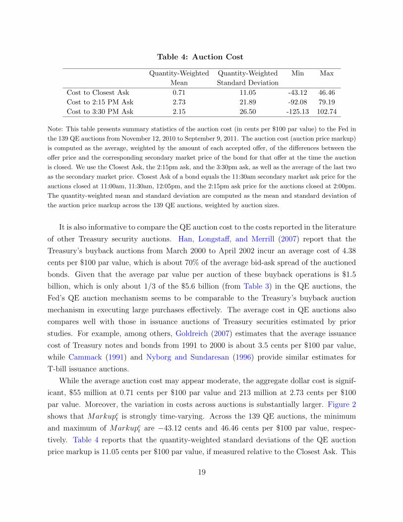
Table 4: Auction Cost
Quantity-Weighted Quantity-Weighted Min Max
Mean Standard Deviation
Cost to Closest Ask 0.71 11.05 -43.12 46.46
Cost to 2:15 PM Ask 2.73 21.89 -92.08 79.19
Cost to 3:30 PM Ask 2.15 26.50 -125.13 102.74
Note: This table presents summary statistics of the auction cost (in cents per $100 par value) to the Fed in
the 139 QE auctions from November 12, 2010 to September 9, 2011. The auction cost (auction price markup)
is computed as the average, weighted by the amount of each accepted offer, of the differences between the
offer price and the corresponding secondary market price of the bond for that offer at the time the auction
is closed. We use the Closest Ask, the 2:15pm ask, and the 3:30pm ask, as well as the average of the last two
as the secondary market price. Closest Ask of a bond equals the 11:30am secondary market ask price for the
auctions closed at 11:00am, 11:30am, 12:05pm, and the 2:15pm ask price for the auctions closed at 2:00pm.
The quantity-weighted mean and standard deviation are computed as the mean and standard deviation of
the auction price markup across the 139 QE auctions, weighted by auction sizes.
It is also informative to compare the QE auction cost to the costs reported in the literature
of other Treasury security auctions. Han, Longstaff, and Merrill (2007) report that the
Treasury’s buyback auctions from March 2000 to April 2002 incur an average cost of 4.38
cents per $100 par value, which is about 70% of the average bid-ask spread of the auctioned
bonds. Given that the average par value per auction of these buyback operations is $1.5
billion, which is only about 1/3 of the $5.6 billion (from Table 3) in the QE auctions, the
Fed’s QE auction mechanism seems to be comparable to the Treasury’s buyback auction
mechanism in executing large purchases effectively. The average cost in QE auctions also
compares well with those in issuance auctions of Treasury securities estimated by prior
studies. For example, among others, Goldreich (2007) estimates that the average issuance
cost of Treasury notes and bonds from 1991 to 2000 is about 3.5 cents per $100 par value,
while Cammack (1991) and Nyborg and Sundaresan (1996) provide similar estimates for
T-bill issuance auctions.
While the average auction cost may appear moderate, the aggregate dollar cost is signif-
icant, $55 million at 0.71 cents per $100 par value and 213 million at 2.73 cents per $100
par value. Moreover, the variation in costs across auctions is substantially larger. Figure 2
shows that Markupct is strongly time-varying. Across the 139 QE auctions, the minimum
and maximum of Markupct are −43.12 cents and 46.46 cents per $100 par value, respec-
tively. Table 4 reports that the quantity-weighted standard deviations of the QE auction
price markup is 11.05 cents per $100 par value, if measured relative to the Closest Ask. This
19
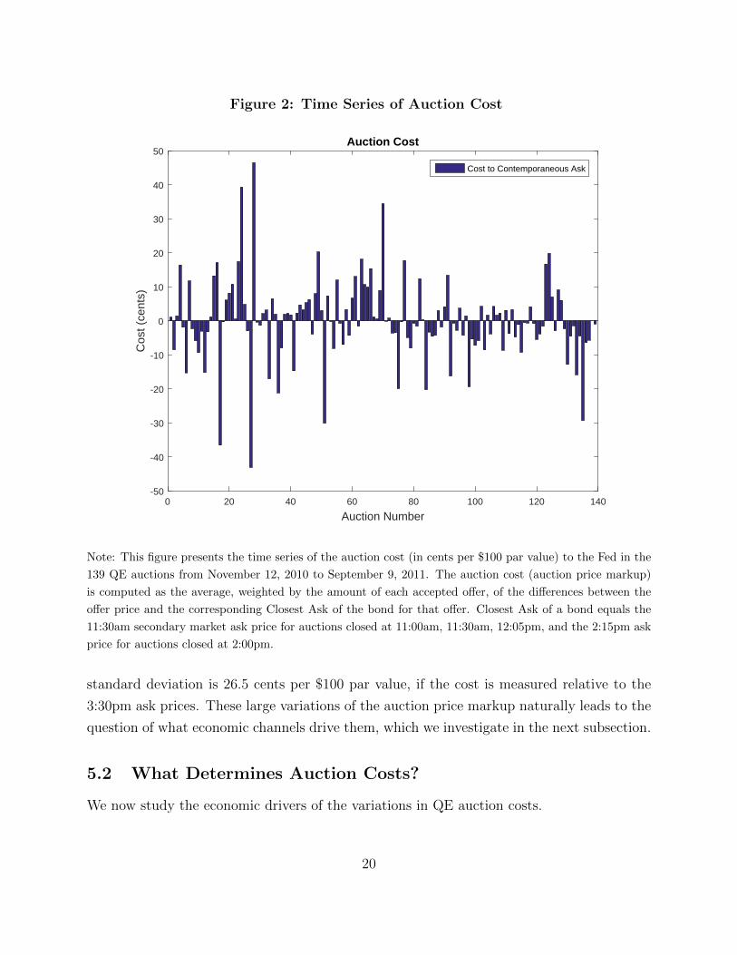
Figure 2: Time Series of Auction Cost
0 20 40 60 80 100 120 140
Auction Number
-50
-40
-30
-20
-10
0
10
20
30
40
50C
ost (
cent
s)Auction Cost
Cost to Contemporaneous Ask
Note: This figure presents the time series of the auction cost (in cents per $100 par value) to the Fed in the
139 QE auctions from November 12, 2010 to September 9, 2011. The auction cost (auction price markup)
is computed as the average, weighted by the amount of each accepted offer, of the differences between the
offer price and the corresponding Closest Ask of the bond for that offer. Closest Ask of a bond equals the
11:30am secondary market ask price for auctions closed at 11:00am, 11:30am, 12:05pm, and the 2:15pm ask
price for auctions closed at 2:00pm.
standard deviation is 26.5 cents per $100 par value, if the cost is measured relative to the
3:30pm ask prices. These large variations of the auction price markup naturally leads to the
question of what economic channels drive them, which we investigate in the next subsection.
5.2 What Determines Auction Costs?
We now study the economic drivers of the variations in QE auction costs.
20
5.2.1 Empirical Measures
As suggested by the stylized model in Section 3, we expect the Fed to pay a higher cost
on bonds whose market prices appear lower than prices implied by the Fed’s internal yield
curve model.
A perfect measure of bond cheapness (from the Fed’s perspective) requires full knowledge
of the exact method used by the Fed to evaluate offers. We do not have such information.
Nonetheless, we will construct a proxy of bond cheapness by applying a popular yield-fitting
model to the NYQS data. Specifically, on each auction day, we first estimate a smooth zero-
coupon yield curve based on observed market prices. This yield curve is then used to price
all bonds purchased in the auction on the auction day. A bond’s cheapness is calculated as
its theoretical price based on our fitted yield curve minus the market ask price. Noise in this
measurement makes it less likely for us to find statistically significant results.
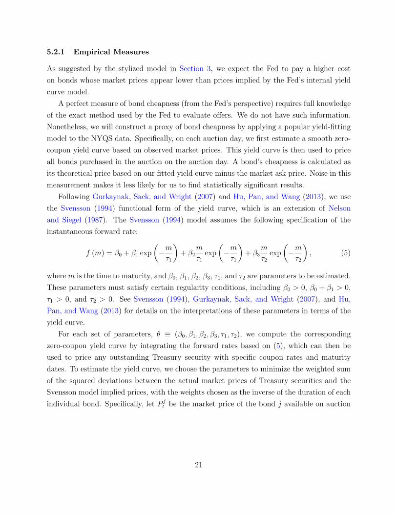
Following Gurkaynak, Sack, and Wright (2007) and Hu, Pan, and Wang (2013), we use
the Svensson (1994) functional form of the yield curve, which is an extension of Nelson
and Siegel (1987). The Svensson (1994) model assumes the following specification of the
instantaneous forward rate:
f (m) = β0 + β1 exp
(−mτ1
)+ β2
m
τ1exp
(−mτ1
)+ β3
m
τ2exp
(−mτ2
), (5)
where m is the time to maturity, and β0, β1, β2, β3, τ1, and τ2 are parameters to be estimated.
These parameters must satisfy certain regularity conditions, including β0 > 0, β0 + β1 > 0,
τ1 > 0, and τ2 > 0. See Svensson (1994), Gurkaynak, Sack, and Wright (2007), and Hu,
Pan, and Wang (2013) for details on the interpretations of these parameters in terms of the
yield curve.
For each set of parameters, θ ≡ (β0, β1, β2, β3, τ1, τ2), we compute the corresponding
zero-coupon yield curve by integrating the forward rates based on (5), which can then be
used to price any outstanding Treasury security with specific coupon rates and maturity
dates. To estimate the yield curve, we choose the parameters to minimize the weighted sum
of the squared deviations between the actual market prices of Treasury securities and the
Svensson model implied prices, with the weights chosen as the inverse of the duration of each
individual bond. Specifically, let P jt be the market price of the bond j available on auction
21

day t, j = 1, · · · , Nt. We choose the parameter θ as
θt = arg minθ
Nt∑j=1
[(P jt (θ)− P j
t
)/Dj
t
]2, (6)
where P jt (θ) is the model-implied price of bond j based on the Svensson model in (5), and Dj
t
is the bond duration. With the parameter estimate θt, we can compute the model-implied
price as P jt (θt) and define the bond cheapness as
Cheapnessjt = P jt (θt)− P j
t , (7)
in unit of cents per $100 par value. The higher is Cheapnessjt , the lower the raw market
price is relative to the theoretical price based on the model estimated using secondary bond
prices, and the cheaper the bond j is according to its quoted market price.
We include in the estimation all outstanding Treasury securities in general, but exclude
those with maturity less than one month. The yields on ultra-short-maturity Treasury bills
may reflect idiosyncratic supply or demand fluctuations beyond the risk-free rate (see Hu,
Pan, and Wang (2013) and Gurkaynak, Sack, and Wright (2007)). We also exclude the most
recently issued “on-the-run” securities because they are usually excluded in QE auctions to
avoid creating supply shortage. But we do include “first off-the-run” bonds (i.e., bonds that
are the second most recently issued in their maturity buckets) because they are eligible for
QE purchases. The market prices we use are the mid-quotes at 8:40am. By construction,
the 8:40am prices are obtained before the auction time and hence not affected by the auction
outcomes. (In the robustness section, we construct alternative measures of cheapness and
find similar results.)
Although we do not observe the Fed’s confidential yield curve model or dealers’ informa-
tion about it, we expect our bond cheapness measure to be positively correlated with that
obtained using the Fed’s model and the dealers’, for two reasons. First, the Svensson (1994)
model is a standard model in fixed income markets. Second, our data on secondary market
prices are obtained from the Fed, and we expect dealers to observe them as well. We caution
that correlated measures do not mean identical measures. We expect some difference among
our cheapness measure, the Fed’s, and the dealers’ because of different sampling time of the
data and the exact set of securities included in the yield-fitting calculation, among others.
Turning to other measures, as mentioned in Section 3, a standard determinant of bidding
behavior is winner’s curse, which in our context could be proxied by the uncertainty of
22

the resale value of the bonds in secondary market. For example, if a dealer sells some
bonds to the Fed, anticipating to cover the short position in the secondary market later,
a higher bond value uncertainty makes this short-covering trade riskier. Thus, we expect
that a higher bond value uncertainty corresponds to a higher cost of the Fed. Following the
literature, we measure bond value uncertainty by the pre-auction volatility V OLjt , computed
as the standard deviation of daily returns of bond j during the five trading days prior to the
auction date t.
Besides cheapness and volatility, we also consider three measures of bond scarcity and
illiqudity: specialness, outstanding balance, and bid-ask spread. Specialness is the difference
between the general repo rate and special repo rate on the CUSIP, in percentage points. The
higher is specialness, the more costly it is for a dealer to locate or finance the bond in the repo
market. Following Han, Longstaff, and Merrill (2007), we define outstanding balance (OBjt )
as the total outstanding par value of the bond j, normalized by the total purchase amount
of auction t, to control for the potential proportionality of auction size to the outstanding
amount. Bid-ask spread (Bid − Askjt ) is the difference between the ask and bid quotes of
bond j, normalized by the mid-quote, denoted in basis points. We use the 8:40am NPQS
quotes when computing bid-ask spread, similar to the calculation of cheapness.
Panel A of Table 5 reports basic summary statistics of these five empirical measures
across both auctions and CUSIPs. We observe that the purchased bonds by the Fed are on
average cheaper than the yield-curve implied value by 25.6 cents per $100 par value, with
a standard deviation of 37.5 cents and median of 12.9 cents. The average daily pre-auction
volatility is 0.37%, and the average specialness is 2.4 basis points. The mean of (normalized)
outstanding balance is 4.99, suggesting that the purchase amount of QE auctions is about
1/5 of the outstanding balance on average. The average bid-ask spread is about 3.5 basis
points for the bonds purchased by the Fed.
Panel B of Table 5 reports the correlation matrix of these five empirical measures, pooled
across all auctions and CUSIPs. Panel C reports the average time-series correlation matrix
by first calculating the correlation for each CUSIP and then averaging across all CUSIPs.
Either way, these five explanatory variables have fairly low correlations in their absolute
values. The only entry whose absolute value is above 0.4 is the correlation between volatility
and normalized outstanding balance, at 0.55. While we do not expect multicollinearity issues
for this reason, in our subsequent regressions we will also run univariate versions just in case.
In Panel D of Table 5 we report the time-series correlations of the daily 2-, 5-, 10-
, and 30-year par yields from our fitted Svensson yield curve with the corresponding par
23

Table 5: Summary Statistics of Empirical Measures
A: Basic Summary Statistics across Auctions and CUSIPs
Cheapness VOL Specialness OB Bid-Ask
Mean 25.621 0.369 0.024 4.991 3.522
Standard Deviation 37.533 0.232 0.027 4.202 1.635
Min -22.668 0.027 -0.027 0.521 0.732
Q - 25% 0.937 0.218 0.009 2.813 2.309
Q - 50% 12.927 0.324 0.016 4.465 3.042
Q - 75% 35.807 0.456 0.030 6.087 4.599
Max 150.682 1.430 0.356 58.806 9.208
B: Pooled Correlations of Empirical Measures
Cheapness 1.000
VOL -0.169 1.000
Specialness -0.047 0.087 1.000
OB -0.016 0.181 -0.042 1.000
Bid-Ask -0.197 0.354 0.172 -0.242 1.000
C: Average Time Series Correlations of Empirical Measures
Cheapness 1.000
VOL -0.081 1.000
Specialness 0.113 0.185 1.000
OB 0.184 0.548 0.244 1.000
Bid-Ask 0.119 0.253 -0.193 -0.123 1.000
D: Yield Curve Correlations with Barclays and GSW
2y 5y 10y 20y 30y
Barclays 0.987 0.992 0.989 0.984 0.979
GSW 0.986 0.992 0.992 0.986 0.981
Note: Panel A reports basic summary statistics of five empirical measures, computed across auctions and
CUSIPs. For each bond in each auction, Cheapness is the difference between the model price implied from
the fitted Svensson yield curve and the actual market mid price (in cents per $100 dollar face value), VOL
is the standard deviation of daily returns of the bond during the five trading days prior to the auction date
(in percentage points), Specialness is the difference between the general repo rate and special repo rate on
the bond (in percentage points), OB is the total outstanding par value of the bond normalized by the total
purchase amount of the auction, and Bid-Ask is the difference between the secondary market ask and bid
quotes of a bond normalized by the mid-quote (in basis points). Panel B reports the correlation matrix of
these five empirical measures by pooling observations across auctions and CUSIPs. Panel C reports their
average time series correlations: a correlation between two measures is computed by first calculating their
sample correlation across auctions for each CUSIP and then averaging across all CUSIPs. Panel D reports
time series correlations of the daily 2-, 5-, 10-, and 30-year par yields from our fitted Svensson yield curve
with those from Barclays as well as from Gurkaynak, Sack, and Wright (2007) (GSW) over our sample
period.
24

yields obtained from Barclays and those from Gurkaynak, Sack, and Wright (2007). The
correlations are very high, around 0.98 or 0.99. These high correlations provide suggestive
evidence that the cheapness measure from our yield curve model is probably correlated with
that from the Fed’s or dealers’ yield curve models.
5.2.2 Regression Results
We now study how the QE auction cost depends on bond cheapness, bond value uncertainty,
and bond scarcity/illiquidity. Our main left-hand variable is the auction price markup mea-
sured to the Closest Ask, but we will also use the price markup relative to the 3:30pm ask
price as a robustness check. For each bond j in each auction t, the CUSIP-level markup is
defined as
Markupt,j =
∑d,o (pt,j,d,o − Pt,j) · qt,j,d,o∑
d,o qt,j,d,o, (8)
where Pt,j is either the Closest Ask or the 3:30pm Ask.
Our empirical analysis is based on the following panel regression of the auction cost for
each bond in each auction on empirical measures of bond cheapness, value uncertainty, and
scarcity/illiquidity:
Markupt,j =∑j
αjDj + β1 · Cheapnesstj + β2 · VOLtj
+β3 · Specialnesstj + β4 ·OBtj + β5 · Bid-Asktj
+β6 · SizeEt + εit, (9)
where CUSIP fixed effect Dj controls for potential unobservable effects generic to individual
bonds. We do not include auction fixed effects because our main objective is to study
the variations of costs across auctions, similar to the literature (such as Han, Longstaff,
and Merrill (2007), Nyborg and Sundaresan (1996), and Hortacsu and Kastl (2012), among
others). Nonetheless, in order to control for the potential effect of the publicly announced
auction size, we include the expected per-CUSIP purchase size SizeEt , computed as the mean
of the announced minimum and maximum of intended purchase amount divided by the
number of included CUSIPs, in $billions of par value.14
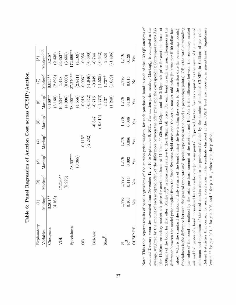
Columns (1)–(5) of Table 6 report results of panel regressions of the auction price markup
14In unreported results, we also include the auction number in the regression as an explanatory variable, inorder to control for the possibility that dealers learn about the bond values or the Fed’s internal spline-basedprices over time (Milgrom and Weber (1982), Ashenfelter (1989), and Han, Longstaff, and Merrill (2007)).We do not find any time trend in the data.
25
relative to Closest Ask, Markupct,j, on the empirical measures of bond cheapness, value
uncertainty, and scarcity/illiquidity, one at a time. We find that, indeed, cheapness affects
the auction price markup positively, consistent with our hypothesis that a higher Fed’s value
for the bonds (relative to market price) is associated with a higher cost. The auction price
markup also has significant and positive loadings on volatility, specialness, and outstanding
balance, implying that bond value uncertainty and bond scarcity/illiquidity increase auction
costs. The result in Column (6) on the multivariate panel regression (9) further confirms the
significance of cheapness, volatility, and specialness (outstanding balance and bid-ask spread
become insignificant).
The economic significance of cheapness is particularly large. According to column (6),
a 37.5 cents increase in cheapness, which is roughly one standard deviation of cheapness
across auctions and CUSIPs in our sample, increases the auction price markup by about
6.3 cents (= 37.5× 0.169) per $100 par value. In comparison, a 0.232 and 0.027 percentage
point increase in volatility and specialness, which are roughly one standard deviation of the
pre-auction volatility and specialness across auction and CUSIP in our sample, respectively,
increases the auction price markup by about 3.8 cents (= 0.232 × 16.5) and 2.1 cents (=
0.027× 78.5) per $100 par value.
The estimates shown in column (7), without CUSIP fixed effects, are still statistically
significant, albeit smaller. Interestingly, as shown in column (8) of Table 6, the magnitudes
of the estimated coefficients are larger if the cost is measured against the 3:30pm Ask.
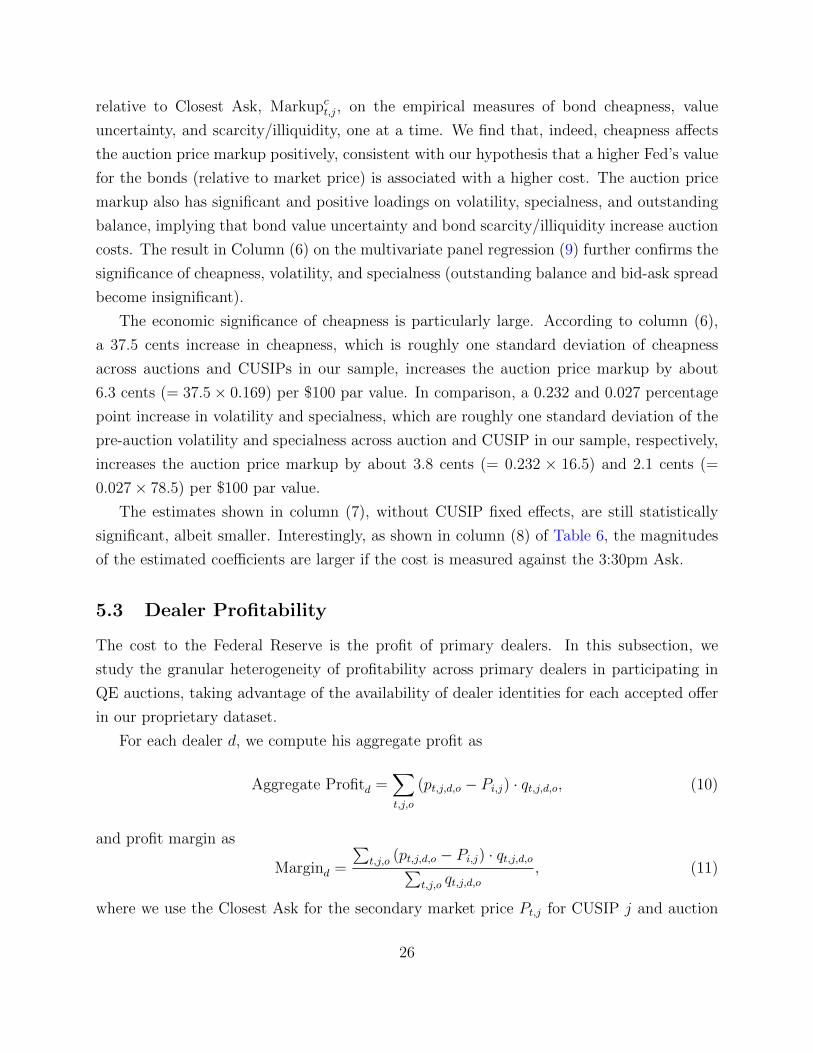
5.3 Dealer Profitability
The cost to the Federal Reserve is the profit of primary dealers. In this subsection, we
study the granular heterogeneity of profitability across primary dealers in participating in
QE auctions, taking advantage of the availability of dealer identities for each accepted offer
in our proprietary dataset.
For each dealer d, we compute his aggregate profit as
Aggregate Profitd =∑t,j,o
(pt,j,d,o − Pi,j) · qt,j,d,o, (10)
and profit margin as
Margind =
∑t,j,o (pt,j,d,o − Pi,j) · qt,j,d,o∑
t,j,o qt,j,d,o, (11)
where we use the Closest Ask for the secondary market price Pt,j for CUSIP j and auction
26
Tab
le6:
Panel
Regre
ssio
nof
Auct
ion
Cost
acr
oss
CU
SIP
/A
uct
ion
Exp
lan
ator
y(1
)(2
)(3
)(4
)(5
)(6
)(7
)(8
)
Var
iab
les
Mar
ku
pc
Mark
upc
Mark
upc
Mark
upc
Mark
upc
Mark
upc
Mark
upc
Mark
up3:3
0
Ch
eap
nes
s0.2
01**
0.16
9**
0.05
5**
0.21
8*
(4.1
65)
(3.1
60)
(2.8
98)
(2.4
38)
VO
L17
.530
**16
.534
**1.
448
23.4
53**
(5.2
26)
(4.9
96)
(0.6
00)
(3.6
55)
Sp
ecia
lnes
s58
.607
**78
.490
**27
.270
**17
2.69
9**
(3.3
65)
(4.5
56)
(2.8
41)
(4.1
69)
OB
-0.1
15*
-0.0
18-0
.093
+-0
.056
(-2.
282)
(-0.
342)
(-1.
946)
(-0.
690)
Bid
-Ask
-0.3
47-0
.716
-0.3
49-0
.744
(-0.
615)
(-1.
276)
(-1.
535)
(-0.
642)
Siz
eE2.
137
1.73
7+
-2.0
28
(1.2
40)
(1.6
59)
(-1.
496)
N1,7
76
1,77
61,
776
1,77
61,
776
1,77
61,
776
1,77
6
R2
0.10
30.
114
0.09
20.
086
0.08
60.
139
0.01
50.
129
CU
SIP
FE
Yes
Yes
Yes
Yes
Yes
Yes
No
Yes
Not
e:T
his
tab
lere
por
tsre
sult
sof
pan
elre
gres
sion
sof
the
au
ctio
np
rice
mark
up
,fo
rea
chp
urc
hase
db
on
din
each
of
the
139
QE
au
ctio
ns
of
nom
inal
Tre
asu
ryse
curi
ties
exec
ute
dfr
omN
ovem
ber
12,
2010
toS
epte
mb
er9,
2011.
Th
eauct
ion
pri
cem
ark
up
Mark
upc t,j
isco
mp
ute
das
the
aver
age,
wei
ghte
dby
the
amou
nt
ofea
chac
cep
ted
off
er,
of
the
diff
eren
ces
bet
wee
nth
eoff
erp
rice
an
dth
eco
rres
pon
din
gC
onte
mp
ora
neo
us
Ask
(th
e11
:30a
mse
cond
ary
mar
ket
ask
pri
cefo
rau
ctio
ns
close
dat
11:0
0am
,11:3
0am
,12:0
5p
m,
an
dth
e2:1
5p
mask
pri
cefo
rau
ctio
ns
close
dat
2:00
pm
)of
the
bon
dfo
rth
atoff
er.
Mar
ku
p3:30
t,j
ism
easu
red
rela
tive
toth
e3:3
0p
mask
pri
ce.
For
each
bon
din
each
au
ctio
n,
Ch
eap
nes
sis
the
diff
eren
ceb
etw
een
the
mod
elp
rice
imp
lied
from
the
fitt
edS
ven
sson
yie
ldcu
rve
an
dth
eact
ual
mark
etm
idp
rice
(in
cents
per
$100
doll
ar
face
valu
e),
VO
Lis
the
stan
dar
dd
evia
tion
ofd
aily
retu
rns
of
the
bon
dd
uri
ng
the
five
trad
ing
day
sp
rior
toth
eau
ctio
nd
ate
(in
per
centa
ge
poin
ts),
Sp
ecia
lnes
sis
the
diff
eren
ceb
etw
een
the
gen
eral
rep
ora
tean
dsp
ecia
lre
po
rate
on
the
bon
d(i
np
erce
nta
ge
poin
ts),
OB
isth
eto
tal
ou
tsta
nd
ing
par
valu
eof
the
bon
dn
orm
aliz
edby
the
tota
lp
urc
hase
am
ou
nt
of
the
au
ctio
n,
an
dB
id-A
skis
the
diff
eren
ceb
etw
een
the
seco
nd
ary
mark
et
ask
and
bid
qu
otes
ofa
bon
dn
orm
aliz
edby
the
mid
-qu
ote
(in
basi
sp
oin
ts).
Exp
ecte
dA
uct
ion
Siz
eis
com
pu
ted
as
the
mea
nof
the
an
nou
nce
d
min
imu
man
dm
axim
um
ofth
eto
tal
auct
ion
am
ount
tob
ep
urc
hase
dd
ivid
edby
the
nu
mb
erof
incl
ud
edC
US
IPs
in$b
illi
on
sof
par
valu
e.
Rob
ust
t-st
atis
tics
that
corr
ect
for
seri
alco
rrel
ati
on
inth
ere
sid
uals
clu
ster
edat
the
CU
SIP
leve
lare
rep
ort
edin
pare
nth
eses
.S
ign
ifica
nce
leve
ls:∗∗
forp<
0.01
,∗
forp<
0.05
,an
d+
forp<
0.1,
wh
erep
isth
ep
-valu
e.
27

t.
Table 7 summarizes the dealer-by-dealer profitability across the 139 QE auctions in our
sample period. Column (1) lists the rankings according to dealers’ aggregate profits, while
the dealer identities are provided in column (2). Columns (3), (4), and (5) provide the
aggregate profit in millions of dollars, the profit margin in cents per $100 par value, and the
aggregate accepted offer amount in billion dollars of par value, respectively. In addition, we
also report the total number of auctions in column (6), the number of winning offers per
auction in column (7), and the total number of CUSIPs sold in column (8).
From columns (3)–(5), we observe a striking concentration of aggregate profits and ag-
gregate amounts of accepted offers among dealers. The top five dealers, Morgan Stanley,
Goldman Sachs, BNP Paribas, J.P. Morgan, and RBC make a combined profit of $59 million,
even larger than the $55.37 million total profit of all dealers, measured relative to the Clos-
est Ask. These five dealers also accounted for about half the $776.6 billion total purchase
amount. Furthermore, the bottom five dealers, RBS, Credit Suisse, UBS, Barclays Capital,
and Citigroup accounted for about 40% of the $776.6 billion total purchase amount, but
their profit margins are much lower. In fact, the bottom five dealers all have negative profit
margins, averaging about −0.44 cents per $100 par value, whereas the top five dealers all
have positive profit margins, averaging 1.67 cents per $100 par value.
In sum, during QE auctions, the intermediation profits in the Treasury market is con-
centrated to only a few dealers. Similar concentration has been documented in other over-
the-counter markets such as municipal bond, corporate bond, and asset-backed securities (Li
and Schurhoff (2014), Di-Maggio, Kermani, and Song (2016), and Hollifield, Neklyudov, and
Spatt (2014)). Furthermore, there is substantial heterogeneity in the profit margins among
dealers who handle similar amounts of intermediation volume. Hence, dealers’ profit margins
in QE auctions seem to be related to economic channels that are orthogonal to their sales
volume.
To link dealers’ profitability to our empirical measures of the determinants of auction
costs, we ask to what extent dealer’s profit margin depends on the dealer’s ability to sell to
the Fed bonds that are cheaper (relative to model), more volatile, or more special. To do
this, we run the following panel regression at the auction-dealer level:
Margint,d =∑d
αdDd + β1 · Cheapnesst,d + β2 · VOLt,d
+β3 · Specialnesst,d + β4 ·OBt,d + β5 · Bid-Askt,d
+β6 · SizeEt + εit, (12)
28

Table
7:
Deale
rP
rofita
bil
ity
(1)
(2)
(3)
(4)
(5)
(6)
(7)
(8)
Ran
kby
Dea
ler
Agg
rega
teP
rofi
tA
ggre
gate
Tota
lN
um
ber
of
Tota
l
Agg
rega
teId
enti
tyP
rofi
tM
arg
inoff
eram
ou
nt
Nu
mb
erof
Win
nin
gO
ffer
sN
um
ber
of
Pro
fit
($m
illi
on)
(Cen
tsp
er$
100)
($b
illi
on
)A
uct
ion
sp
erA
uct
ion
Win
nin
gC
US
IPs
1M
orga
nS
tan
ley
22.6
71.8
0125.8
8128
6129
2G
old
man
Sac
hs
19.3
01.3
4143.6
1138
12
147
3B
NP
Par
ibas
l7.
611.5
748.4
9131
32
174
4J.P
.M
orga
n6.
451.9
632.9
1131
5137
5R
BC
2.97
1.6
617.9
2103
4127
6M
erri
llL
yn
ch2.
261.3
516.7
8114
5130
7D
aiw
a1.
772.0
48.7
189
381
8H
SB
C1.
670.7
422.5
5117
3114
9Jeff
erie
s1.
220.9
412.9
2116
3108
10N
omu
ra0.
680.3
619.0
8116
3117
11D
euts
che
Ban
k0.
570.2
424.2
4113
5125
12C
anto
rF
itzg
eral
d0.
360.6
25.8
0101
396
13M
izu
ho
-0.1
9-0
.41
4.7
490
380
14S
GA
mer
icas
-0.2
1-0
.56
3.7
751
245
15M
FG
lob
al-0
.34
-1.5
32.2
140
244
16R
BS
-0.6
3-0
.11
59.2
7120
5120
17C
red
itS
uis
se-0
.72
-0.0
982.9
7132
6140
18U
BS
-0.8
-0.3
125.6
1106
4117
19B
arcl
ays
Cap
ita
-2.7
7-0
.469.5
7131
7144
20C
itig
rou
p-6
.50
-1.3
149.6
1124
5135
Ave
rage
2.77
0.5
038.8
3110
6116
Not
e:T
his
tab
lesu
mm
ariz
esth
ed
eale
rp
rofi
tab
ilit
yacr
oss
the
139
QE
au
ctio
ns
of
nom
inal
Tre
asu
ryse
curi
ties
from
Nov
emb
er12,
2010
to
Sep
tem
ber
9,20
11.
For
each
dea
ler,
we
com
pu
teth
ep
rofi
tm
arg
inas
the
aver
age
(wei
ghte
dby
the
am
ou
nt
of
each
acc
epte
doff
er)
of
the
diff
eren
ces
bet
wee
nth
eoff
erp
rice
and
the
corr
esp
on
din
gC
lose
stA
sk(t
he
11:3
0am
seco
nd
ary
mark
etask
pri
cefo
rth
eau
ctio
ns
close
dat
11:0
0am
,11
:30a
m,
12:0
5pm
,an
dth
e2:
15p
mas
kp
rice
for
the
au
ctio
ns
close
dat
2:0
0p
m)
for
the
bon
dof
that
off
er,
for
each
dea
ler
acr
oss
all
auct
ion
s.T
he
aggr
egat
ep
rofi
tof
each
dea
ler
isco
mp
ute
das
the
pro
du
ctb
etw
een
the
pro
fit
marg
inan
dto
tal
off
eram
ou
nt
the
dea
ler
sold
to
the
Fed
.W
era
nk
the
dea
lers
acco
rdin
gto
thei
raggre
gate
pro
fits
,an
dre
port
the
corr
esp
on
din
gra
nkin
gs,
dea
ler
iden
titi
es,
aggre
gate
pro
fits
in$
mil
lion
s,p
rofi
tm
argi
ns
ince
nts
per
$100
par
valu
e,aggre
gate
off
eram
ou
nt
in$
bil
lion
sof
par
valu
eso
ldto
the
Fed
,to
tal
nu
mb
erof
auct
ion
s,nu
mb
erof
win
nin
goff
ers
per
auct
ion
,an
dto
tal
nu
mb
erof
CU
SIP
sso
ld.
29

where the profit margin Margint,d of dealer d in auction t is computed as
Margint,d =
∑j,o (pt,j,d,o − Pi,j) · qt,j,d,o∑
j,o qt,j,d,o, (13)
and the secondary market price Pt,j for CUSIP j of auction t is the Closest Ask. In regression
(12), the empirical measures Cheapnesst,d, VOLt,d, Specialnesst,d, OBt,d, and Bid-Askt,d are
calculated as the average of the respective measures of each purchased CUSIP for each
winning dealer d in each auction t, weighted by this dealer’s purchase amount of this CUSIP
in auction t. Therefore, Cheapnesst,d measures the average cheapness of the bonds dealer d
sold to the Fed in auction t, and similarly for other measures. We include the dealer fixed
effect Dd to control for potential unobservable effects generic to dealers, but do not include
auction fixed effects because our main objective is to study the variations of costs across
auctions, similar to (9). We also control for the potential auction size effect by including the
expected per-CUSIP auction size SizeEt .
Literally, the coefficient β1 reflects the degree of heterogeneity in the average cheapness
of the bonds that different dealers sell to the Fed. Similar interpretations apply to the other
coefficients.
Table 8 reports the results. In columns (1)–(6), the univariate and multivariate regres-
sions show that the dealer profit margin Marginct,d is significantly higher if the dealer-specific
cheapness measure is higher. In particular, from column (6), a 29 cent per $100 par value in-
crease in cheapness, which is roughly one standard deviation of cheapness across auction and
dealer in our sample, increases the dealer’s profit margin by about 3.8 cents (= 29× 0.132)
per $100 par value. A 0.022 percentage point increase in specialness, which is roughly one
standard deviation of specialness across auctions and dealers in our sample, increase the
dealer’s profit margin by about 0.63 cents (= 0.022 × 28.451) per $100 par value. The
coefficient for volatility, however, is insignificant.
Columns (7) and (8) show robustness of the main results. Interestingly, the estimates
in column (7), where dealer fixed effects are excluded from the right-hand side, are almost
identical to those in column (6). In column (8), where costs are measured relative to the
3:30pm Ask, the coefficient for cheapness remains significant, albeit smaller.
30
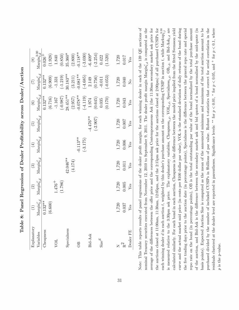
Table
8:
Panel
Regre
ssio
nof
Deale
rP
rofita
bil
ity
acr
oss
Deale
r/A
uct
ion
Exp
lan
ator
y(1
)(2
)(3
)(4
)(5
)(6
)(7
)(8
)
Var
iab
les
Mar
ginc t,d
Marg
inc t,d
Marg
inc t,d
Marg
inc t,d
Marg
inc t,d
Marg
inc t,d
Marg
inc t,d
Marg
in3:30
t,d
Ch
eap
nes
s0.
132**
0.13
2**
0.13
2**
0.02
6+
(6.6
00)
(6.7
16)
(6.9
09)
(1.9
28)
VO
L1.
476+
-1.1
67-1
.331
1.84
0
(1.7
86)
(-0.
987)
(-1.
219)
(0.8
50)
Sp
ecia
lnes
s42
.046
**28
.451
**30
.183
**35
.360
*
(4.1
74)
(2.9
57)
(3.2
11)
(2.8
00)
OB
-0.1
13**
-0.0
78**
-0.0
81**
-0.1
18**
(-3.
175)
(-4.
119)
(-4.
685)
(-3.
030)
Bid
-Ask
-4.4
76**
1.97
42.
149
-6.4
09*
(-2.
907)
(0.6
45)
(0.7
56)
(-2.
254)
Siz
eE0.
035
-0.0
110.
422
(0.1
70)
(-0.
053)
(1.5
20)
N1,
720
1,72
01,
720
1,72
01,
720
1,72
01,
720
1,72
0
R2
0.0
370.
005
0.01
10.
006
0.00
70.
043
0.04
00.
017
Dea
ler
FE
Yes
Yes
Yes
Yes
Yes
Yes
No
Yes
Not
e:T
his
tab
lere
por
tsre
sult
sof
pan
elre
gres
sion
sof
the
dea
ler
pro
fit
marg
in,
for
each
win
nin
gd
eale
rin
each
of
the
139
QE
au
ctio
ns
of
nom
inal
Tre
asu
ryse
curi
ties
exec
ute
dfr
omN
ovem
ber
12,
2010
toS
epte
mb
er9,
2011.
Th
ed
eale
rp
rofi
tm
arg
inM
arg
inc t,d
isco
mpu
ted
as
the
aver
age
ofth
ed
iffer
ence
sb
etw
een
the
offer
pri
cean
dth
eco
rres
pon
din
gC
onte
mp
ora
neo
us
Ask
(th
e11:3
0am
seco
nd
ary
mark
etask
pri
cefo
r
the
auct
ion
scl
osed
at11
:00a
m,
11:3
0am
,12
:05p
m,
an
dth
e2:1
5p
mask
pri
cefo
rth
eau
ctio
ns
close
dat
2:0
0p
m)
of
all
pu
rch
ase
dC
US
IPs
for
each
win
nin
gd
eale
rd
inea
chau
ctio
nt,
wei
ghte
dby
this
dea
ler’
sp
urc
hase
am
ou
nt
on
the
corr
esp
ond
ing
CU
SIP
inau
ctio
nt,
wh
ile
Mark
up3:30
t,j
ism
easu
red
rela
tive
toth
e3:
30p
mas
kp
rice
.T
he
exp
lan
ato
ryva
riab
les,
Ch
eap
nes
s t,d
,V
OLt,d,
Sp
ecia
lnes
s t,d
,O
Bt,d,
an
dB
id-A
skt,d
are
calc
ula
ted
sim
ilar
ly.
For
each
bon
din
each
auct
ion
,C
hea
pn
ess
isth
ed
iffer
ence
bet
wee
nth
em
od
elp
rice
imp
lied
from
the
fitt
edS
ven
sson
yie
ld
curv
ean
dth
eac
tual
mar
ket
mid
pri
ce(i
nce
nts
per
$100
doll
ar
par
valu
e),
VO
Lis
the
stan
dard
dev
iati
on
of
dail
yre
turn
sof
the
bon
dd
uri
ng
the
five
trad
ing
day
sp
rior
toth
eau
ctio
nd
ate
(in
per
centa
ge
poin
ts),
Sp
ecia
lnes
sis
the
diff
eren
ceb
etw
een
the
gen
eral
rep
ora
tean
dsp
ecia
l
rep
ora
teon
the
bon
d(i
np
erce
nta
gep
oints
),O
Bis
the
tota
lou
tsta
nd
ing
par
valu
eof
the
bon
dn
orm
ali
zed
by
the
tota
lp
urc
hase
am
ou
nt
ofth
eau
ctio
n,
and
Bid
-Ask
isth
ed
iffer
ence
bet
wee
nth
ese
con
dary
mark
etask
an
db
idqu
ote
sof
ab
on
dn
orm
ali
zed
by
the
mid
-qu
ote
(in
bas
isp
oints
).E
xp
ecte
dA
uct
ion
Siz
eis
com
pu
ted
as
the
mea
nof
the
an
nou
nce
dm
inim
um
an
dm
axim
um
of
the
tota
lau
ctio
nam
ou
nt
tob
e
pu
rch
ased
div
ided
by
the
nu
mb
erof
incl
ud
edC
US
IPs
in$b
illi
on
sof
par
valu
e.R
ob
ust
t-st
ati
stic
sth
at
corr
ect
for
seri
al
corr
elati
on
inth
e
resi
du
als
clu
ster
edat
the
dea
ler
leve
lar
ere
por
ted
inp
are
nth
eses
.S
ign
ifica
nce
leve
ls:∗∗
forp<
0.01,∗
forp<
0.05,
an
d+
forp<
0.1,
wh
ere
pis
the
p-v
alu
e.
31

6 Additional Results and Robustness
In this section, we provide additional results and robustness checks on our main empirical
finding of the determinants of QE auction costs.
6.1 Controlling for Purchase Amount
As mentioned before, our measure of auction costs are realized costs–purchase price at auc-
tion time minus market prices some time after the auction. One may suspect that the auction
outcome itself may affect the measured cost by affecting the secondary market prices after
the auction. To mitigate this concern, we explicitly control for the effect of published quan-
tity by adding q11am,j,d,o to our baseline regression (9). Columns (1)-(6) of Table 9 report
these regression results. We observe that cheapness, volatility, and specialness all remain
highly significant, with similar magnitude as in the baseline specification. Moreover, column
(7) reports the regression of the auction purchase quantity on the same set of explanatory
variables. We observe no significant loadings on cheapness and specialness, suggesting that
the Fed does not purchase more bonds that look cheaper or more special. But there is a
positive loading on volatility and a negative loading on bid-ask spread. Overall, our main
results on the economic determinants of auction costs are robust to the slightly lagged timing
of the auction price markup measure.15
6.2 Alternative Cheapness Measures
Recall from equation (7) that our baseline bond cheapness measure is Cheapnessjt = P jt (θt)−
P jt , where P j
t (θt) is the theoretical price based on the Svensson model estimated using all
available bond (mid) prices, and P jt is the market price. We now provide evidence on the
robustness of our main results to alternative measures of bond cheapness.
First of all, since Cheapnessjt is measured in cents per $100 par value, it may be mechan-
ically larger in magnitude for expensive bonds such as long-term bonds with high coupon
rates. To alleviate this concern, we construct two alternative measures of bond cheapness.
The first normalizes Cheapnessjt by the market price P jt , while the second transforms the
prices P jt and P j
t (θt) into par yields and then takes the yield difference. Columns (1)-(4)
of Table 10 report results of our main regression (9) using these two alternative measures
of bond cheapness. Both univariate and multivariate regressions confirm the results in the
15We are grateful to Stefania D’Amico for pointing out these potential issues.
32
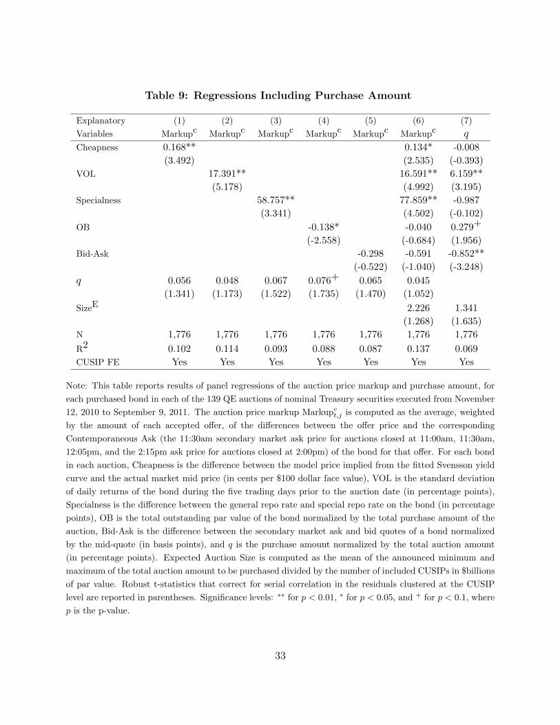
Table 9: Regressions Including Purchase Amount
Explanatory (1) (2) (3) (4) (5) (6) (7)
Variables Markupc Markupc Markupc Markupc Markupc Markupc qCheapness 0.168** 0.134* -0.008
(3.492) (2.535) (-0.393)
VOL 17.391** 16.591** 6.159**
(5.178) (4.992) (3.195)
Specialness 58.757** 77.859** -0.987
(3.341) (4.502) (-0.102)
OB -0.138* -0.040 0.279+
(-2.558) (-0.684) (1.956)
Bid-Ask -0.298 -0.591 -0.852**
(-0.522) (-1.040) (-3.248)
q 0.056 0.048 0.067 0.076+ 0.065 0.045
(1.341) (1.173) (1.522) (1.735) (1.470) (1.052)
SizeE 2.226 1.341
(1.268) (1.635)
N 1,776 1,776 1,776 1,776 1,776 1,776 1,776
R2 0.102 0.114 0.093 0.088 0.087 0.137 0.069
CUSIP FE Yes Yes Yes Yes Yes Yes Yes
Note: This table reports results of panel regressions of the auction price markup and purchase amount, for
each purchased bond in each of the 139 QE auctions of nominal Treasury securities executed from November
12, 2010 to September 9, 2011. The auction price markup Markupct,j is computed as the average, weighted
by the amount of each accepted offer, of the differences between the offer price and the corresponding
Contemporaneous Ask (the 11:30am secondary market ask price for auctions closed at 11:00am, 11:30am,
12:05pm, and the 2:15pm ask price for auctions closed at 2:00pm) of the bond for that offer. For each bond
in each auction, Cheapness is the difference between the model price implied from the fitted Svensson yield
curve and the actual market mid price (in cents per $100 dollar face value), VOL is the standard deviation
of daily returns of the bond during the five trading days prior to the auction date (in percentage points),
Specialness is the difference between the general repo rate and special repo rate on the bond (in percentage
points), OB is the total outstanding par value of the bond normalized by the total purchase amount of the
auction, Bid-Ask is the difference between the secondary market ask and bid quotes of a bond normalized
by the mid-quote (in basis points), and q is the purchase amount normalized by the total auction amount
(in percentage points). Expected Auction Size is computed as the mean of the announced minimum and
maximum of the total auction amount to be purchased divided by the number of included CUSIPs in $billions
of par value. Robust t-statistics that correct for serial correlation in the residuals clustered at the CUSIP
level are reported in parentheses. Significance levels: ∗∗ for p < 0.01, ∗ for p < 0.05, and + for p < 0.1, where
p is the p-value.
33

baseline specification.
Second, we compute Cheapnessjt using alternative inputs of secondary market bond prices
in fitting the Svensson model, including ask prices (instead of mid prices), all bonds with
maturities longer than a year (instead of all bonds except those on-the-run or with maturity
less than a month), and the 3:30pm bond prices one day before the auction (instead of bond
prices at 8:40am on the auction day). Columns (5)-(10) of Table 10 report results of the
main regression (9) using these three alternative measures. We find the results to be similar
to the baseline specification.
Third, we compute Cheapnessjt using a spline method (i.e. piecewise-defined polynomi-
als) with a roughness penalty function of Fisher, Nychka, and Zervos (1995) that balances
the goodness-of-fit and the smoothness of the forward yield curve. Columns (11)-(12) of
Table 10 report results of the main regression (9) using the spline-based bond cheapness
measure. Again, the results are similar to the baseline specification.
6.3 Time Series Controls
As discussed in Section 5.2.2, our baseline regression (9) controls for the expected per-
CUSIP purchase size. One may be concerned that other time-series variations, such as those
in interest rates and interest rate volatilities, can drive variations of auction costs over time.
For example, Figure 2 seems to suggest that the variations in auction costs may be decreasing
over time.
We conduct a robustness check by including, as control variables, 2-year, 5-year, and 10-
year zero-coupon Treasury yields, denoted y(2), y(5), and y(10), as well as at-the-money
swaption implied volatilities of 2-year, 5-year, and 10-year swap rates, denoted SIV(2),
SIV(5), and SIV(10). The series of zero-coupon yields are from Gurkaynak, Sack, and Wright
(2007), whereas those of three-month swaption implied volatilities are from Barclays. The
results are reported in Table 11. As before, we find that the coefficients for cheapness,
volatility, and specialness remains similar to the baseline specification.
34
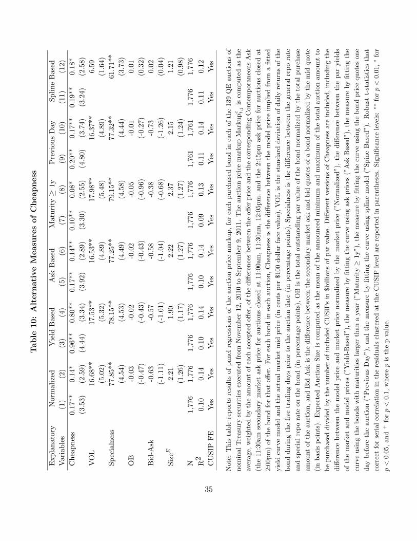
Tab
le10:
Alt
ern
ati
ve
Measu
res
of
Cheapness
Exp
lan
ato
ryN
orm
aliz
edY
ield
Bas
edA
skB
ased
Mat
uri
ty≥
1yP
revio
us
Day
Sp
lin
eB
ased
Var
iab
les
(1)
(2)
(3)
(4)
(5)
(6)
(7)
(8)
(9)
(10)
(11)
(12)
Ch
eap
nes
s0.
17**
0.14
*0.9
6**
0.80
**0.
17**
0.14
**0.
10**
0.08
*0.
20**
0.17
**0.
19**
0.18
*
(3.5
3)
(2.5
9)(4
.44)
(3.3
4)(3
.92)
(2.8
9)(3
.30)
(2.5
5)(4
.80)
(3.7
4)(3
.24)
(2.5
8)
VO
L16
.68**
17.5
3**
16.5
3**
17.9
8**
16.3
7**
6.59
(5.0
2)
(5.3
2)(4
.89)
(5.4
8)(4
.89)
(1.6
4)
Sp
ecia
lnes
s77
.85**
78.1
5**
77.2
5**
79.1
5**
77.3
2**
61.7
1**
(4.5
4)
(4.5
3)(4
.49)
(4.5
8)(4
.44)
(3.7
3)
OB
-0.0
3-0
.02
-0.0
2-0
.05
-0.0
10.
01
(-0.
47)
(-0.
43)
(-0.
43)
(-0.
96)
(-0.
27)
(0.3
2)
Bid
-Ask
-0.6
3-0
.57
-0.5
8-0
.38
-0.7
30.
02
(-1.
11)
(-1.
01)
(-1.
04)
(-0.
68)
(-1.
26)
(0.0
4)
Siz
eE2.2
11.
902.
222.
372.
151.
21
(1.2
6)
(1.1
7)(1
.27)
(1.2
7)(1
.24)
(0.9
8)
N1,
776
1,77
61,
776
1,77
61,
776
1,77
61,
776
1,77
61,
761
1,76
11,
776
1,77
6
R2
0.10
0.1
40.1
00.
140.
100.
140.
090.
130.
110.
140.
110.
12
CU
SIP
FE
Yes
Yes
Yes
Yes
Yes
Yes
Yes
Yes
Yes
Yes
Yes
Yes
Not
e:T
his
tab
lere
por
tsre
sult
sof
pan
elre
gres
sion
sof
the
au
ctio
np
rice
mark
up
,fo
rea
chp
urc
hase
db
on
din
each
of
the
139
QE
au
ctio
ns
of
nom
inal
Tre
asu
ryse
curi
ties
exec
ute
dfr
omN
ovem
ber
12,
2010
toS
epte
mb
er9,
2011.
Th
eauct
ion
pri
cem
ark
up
Mark
upc t,j
isco
mp
ute
das
the
aver
age,
wei
ghte
dby
the
amou
nt
ofea
chac
cep
ted
off
er,
of
the
diff
eren
ces
bet
wee
nth
eoff
erp
rice
an
dth
eco
rres
pon
din
gC
onte
mp
ora
neo
us
Ask
(th
e11
:30a
mse
cond
ary
mar
ket
ask
pri
cefo
rau
ctio
ns
close
dat
11:0
0am
,11:3
0am
,12:0
5p
m,
an
dth
e2:1
5p
mask
pri
cefo
rau
ctio
ns
close
dat
2:00
pm
)of
the
bon
dfo
rth
atoff
er.
For
each
bon
din
each
au
ctio
n,
Ch
eap
nes
sis
the
diff
eren
ceb
etw
een
the
mod
elp
rice
imp
lied
from
afi
tted
yie
ldcu
rve
mod
elan
dth
eac
tual
mar
ket
mid
pri
ce(i
nce
nts
per
$100
doll
ar
face
valu
e),
VO
Lis
the
stan
dard
dev
iati
on
of
daily
retu
rns
of
the
bon
dd
uri
ng
the
five
trad
ing
day
sp
rior
toth
eau
ctio
nd
ate
(in
per
centa
ge
poin
ts),
Sp
ecia
lnes
sis
the
diff
eren
ceb
etw
een
the
gen
eral
rep
ora
te
and
spec
ial
rep
ora
teon
the
bon
d(i
np
erce
nta
ge
poin
ts),
OB
isth
eto
tal
ou
tsta
nd
ing
par
valu
eof
the
bon
dn
orm
ali
zed
by
the
tota
lp
urc
hase
amou
nt
ofth
eau
ctio
n,
and
Bid
-Ask
isth
ed
iffer
ence
bet
wee
nth
ese
con
dary
mark
etask
an
dbid
qu
ote
sof
ab
on
dn
orm
ali
zed
by
the
mid
-qu
ote
(in
bas
isp
oints
).E
xp
ecte
dA
uct
ion
Siz
eis
com
pu
ted
as
the
mea
nof
the
an
nou
nce
dm
inim
um
an
dm
axim
um
of
the
tota
lau
ctio
nam
ou
nt
to
be
pu
rchas
edd
ivid
edby
the
nu
mb
erof
incl
ud
edC
US
IPs
in$b
illion
sof
par
valu
e.D
iffer
ent
ver
sion
sof
Ch
eap
nes
sare
incl
ud
ed,
incl
ud
ing
the
diff
eren
ceb
etw
een
the
mod
elp
rice
and
mar
ket
pri
cen
orm
ali
zed
by
the
mark
etp
rice
(”N
orm
ali
zed
”),
the
diff
eren
ceb
etw
een
the
par
yie
lds
ofth
em
arke
tan
dm
od
elp
rice
s(”
Yie
ld-B
ased
”),
the
mea
sure
by
fitt
ing
the
curv
eu
sin
gask
pri
ces
(”A
skB
ase
d”),
the
mea
sure
by
fitt
ing
the
curv
eu
sin
gth
eb
ond
sw
ith
mat
uri
ties
larg
erth
an
ayea
r(”
Matu
rity≥
1y”),
the
mea
sure
by
fitt
ing
the
curv
eu
sin
gth
eb
on
dp
rice
qu
ote
son
e
day
bef
ore
the
auct
ion
(”P
revio
us
Day
”),
and
the
mea
sure
by
fitt
ing
the
curv
eu
sin
gsp
lin
em
od
el(”
Sp
ine
Base
d”).
Rob
ust
t-st
ati
stic
sth
at
corr
ect
for
seri
alco
rrel
atio
nin
the
resi
du
als
clu
ster
edat
the
CU
SIP
leve
lare
rep
ort
edin
pare
nth
eses
.S
ign
ifica
nce
leve
ls:∗∗
forp<
0.0
1,∗
for
p<
0.05
,an
d+
forp<
0.1,
wh
erep
isth
ep
-valu
e.
35

Table 11: Time Series Controls
Explanatory (1) (2) (3) (4) (5) (6) (7)
Variables Markupc Markupc Markupc Markupc Markupc Markupc Markupc
Cheapness 0.178** 0.170* 0.187** 0.183** 0.189** 0.193** 0.171*
(2.773) (2.482) (2.865) (2.635) (2.848) (2.817) (2.592)
VOL 15.564** 15.083** 12.916** 15.871**
(3.496) (3.196) (2.793) (3.744)
Specialness 52.227** 55.077** 55.574** 48.354**
(3.213) (3.365) (3.418) (2.954)
SizeE 1.144 0.456 1.209+ 0.391 1.122 0.242 0.440
(1.599) (0.553) (1.709) (0.502) (1.630) (0.338) (0.506)
y(2) 7.550** 7.929** 57.688**
(2.989) (3.115) (3.401)
SIV(2) -6.585** -12.397** -24.322**
(-2.625) (-4.869) (-3.837)
y(5) 2.577* 1.763 -39.906**
(2.401) (1.636) (-3.943)
SIV(5) -5.350 -17.979** 6.509
(-1.078) (-3.621) (0.460)
y(10) 2.907* 1.919+ 17.882**
(2.478) (1.695) (3.943)
SIV(10) -6.007 -21.144** -4.811
(-0.782) (-2.838) (-0.408)
N 1,757 1,757 1,757 1,757 1,757 1,757 1,757
R2 0.135 0.151 0.129 0.144 0.129 0.142 0.168
CUSIP FE Yes Yes Yes Yes Yes Yes Yes
Note: This table reports panel regressions of the auction price markup, for each purchased bond in each
of the 139 QE auctions of nominal Treasury securities executed from November 12, 2010 to September 9,
2011. The auction price markup Markupct,j is computed as the average, weighted by the amount of each
accepted offer, of the differences between the offer price and the corresponding Contemporaneous Ask (the
11:30am secondary market ask price for auctions closed at 11:00am, 11:30am, 12:05pm, and the 2:15pm ask
price for auctions closed at 2:00pm) of the bond for that offer. For each bond in each auction, Cheapness is
the difference between the model price implied from the fitted Svensson yield curve and the actual market
mid price (in cents per $100 dollar face value), VOL is the standard deviation of daily returns of the bond
during the five trading days prior to the auction date (in percentage points), and Specialness is the difference
between the general repo rate and special repo rate on the bond (in percentage points). Expected Auction
Size is computed as the mean of the announced minimum and maximum of the total auction amount to
be purchased divided by the number of included CUSIPs in $billions of par value. The 2-, 5-, and 10-year
Treasury yields (y(2), y(5), and y(10), respectively) as well as three-month swaption implied volatilities on
2-, 5-, and 10-year swap rates (SIV (2), SIV (5), and SIV (10), respectively) are included as controls. Robust
t-statistics that correct for serial correlation in the residuals clustered at the CUSIP level are reported in
parentheses. Significance levels: ∗∗ for p < 0.01, ∗ for p < 0.05, and + for p < 0.1, where p is the p-value.
36

7 Conclusion
Since the global financial crisis, central banks around the world have implemented aggres-
sive quantitative easing. This paper provides the first empirical analysis of QE auctions, the
unique mechanism that implements QE in the U.S. Treasury markets. A unique feature of
QE auctions, relative to issuance auctions, is that the Fed evaluates offers on multiple, sub-
stitutable bonds based on internal benchmark prices. The transparency of such mechanism
makes the Fed’s relative values partly predictable.
In our sample period of November 2010 to September 2011, the Federal Reserve purchased
$780 billion Treasury securities. Using a proprietary dataset that contains details of each
winning offer in each QE auction, we find that the Fed pays 0.71–2.73 cents per $100 par
value above the secondary market ask prices. We further show that the cost of buying a bond
in QE auctions has a significant and economically large loading on bond “cheapness”—how
much the bond market price is below a yield-curve-model-implied value. A higher volatility
or specialness is also associated with a higher cost. Moreover, we find great heterogeneity of
profit margins across dealers with comparable selling amounts. Our evidence suggests that
dealers seem to have information about the relative valuations of the Fed on multiple bonds.
A possible direction of future research is to consider possible improvement of QE auc-
tions, or study the optimal mechanism for implementing QE purchases. This direction re-
mains highly relevant to the extent that central banks may continue using QE in the future.
One approach is to estimate dealers’ supply curves and conduct counterfactual analysis of
alternative auction design. But such an analysis is likely to require data on dealers’ offers
that are rejected by the Fed, which we do not have. We thus leave this task for future
research.
37
References
Ashenfelter, O. 1989. How auctions work for wine and art. Journal of Economic Perspectives3: 23–36.
Ausubel, L., Cramton, P., Pycia, M., Rostek, M., and Weretka, M. 2013. Demand Reductionand Inefficiency in Multi-Unit Auctions. Working paper. .
Back, K., and Zender, J. 1993. Auctions of divisible goods: On the rationale for the Treasuryexperiment. Review of Financial Studies 6: 733–764.
Bauer, M., and Rudebusch, G. 2013. The Signaling Channel for Federal Reserve Bond Pur-chases. International Journal of Central Banking forthcoming.
Bikhchandani, S., and Huang, C. 1989. Auctions with Resale Markets: A Model of TreasuryBill Auctions. Review of Financial Studies 2: 311–340.
Bikhchandani, S., and Huang, C. 1993. The economics of Treasury securities markets. Journalof Economic Perspectives 7: 117–134.
Cammack, E. 1991. Evidence on bidding strategies and the information in Treasury billauctions. Journal of Political Economy 99: 100–130.
Chatterjee, A., and Jarrow, R. 1998. Market manipulation, price bubbles, and a model ofthe US Treasury securities auction market. Journal of Financial and Quantitative Analysis33: 255–290.
Christensen, J., and Rudebusch, G. 2012. The Response of Interest Rates to US and UKQuantitative Easing. Economic Journal 122: 385–414.
D’Amico, S., English, W., Lopez-Salido, D., and Nelson, E. 2012. The Federal Reserve’sLarge-Scale Asset Purchase Programs: Rationale and Efects. Economic Journal 122: 415–226.
D’Amico, S., Fan, R., and Kitsul, Y. 2013. The Scarcity Value of Treasury Collateral: RepoMarket Effects of Security-Specific Supply and Demand Factors. Federal Reserve Bank ofChicago, Woking Paper No. 2013-22.
D’Amico, S., and King, T. 2013. Flow and Stock Effects of Large-Scale Treasury Purchases:Evidence on the Importance of Local Supply. Journal of Financial Economics 108: 425–448.
Di-Maggio, M., Kermani, A., and Song, Z. 2016. The Value of Trading Relationships inTurbulent Times. Journal of Financial Economics (forthcoming).
Duarte, J., Longstaff, F., and Yu, F. 2007. Risk and Return in Fixed Income Arbitrage:Nickels in Front of a Steamroller?. Review of Financial Studies pp. 769–811.
38
Duffie, D. 1996. Special repo rates. Journal of Finance 51: 493–526.
Engle, R., Fleming, M., Ghysels, E., and Nguyen, G. 2012. Liquidity, Volatility, and Flightsto Safety in the U.S. Treasury Market: Evidence from a New Class of Dynamic OrderBook Models. Federal Reserve Bank of New York Staff Reports no. 590.
Eser, F., and Schwaab, B. 2016. Evaluating the impact of unconventional monetary policymeasures: Empirical evidence from the ECB’s Securities Markets Programme. Journal ofFinancial Economics 119: 147–167.
Fisher, M., Nychka, D., and Zervos, D. 1995. Fitting the term structure of interest rateswith smoothing splines. Finance and Economics Discussion Series, Board of Governorsof the Federal Reserve System 1.
Fleming, M., and Mizrach, B. 2009. The Microstructure of a U.S. Treasury ECN: TheBrokderTech Platform. Federal Reserve Bank of New York Staff Reports no. 381.
Gagnon, J., Raskin, M., Remanche, J., and Sack, B. 2011. The Financial Market Effectsof the Federal Reserve’s Large-Scale Asset Purchases. International Journal of CentralBanking 7-1: 3–44.
Goldreich, D. 2007. Underpricing in discriminatory and uniform-price Treasury auctions.Journal of Financial and Quantitative Analysis 42 (2): 443–466.
Gordy, M. 1999. Hedging Winner’s Curse with Multiple Bids: Evidence from the PortugueseTreasury Bill Auction. Review of Economics and Statistics 81: 448–465.
Goswami, G., Noe, T., and Rebello, M. 1996. Collusion in Uniform-Price Auctions: Experi-mental Evidence and Implications for Treasury Auctions. Review of Financial Studies 9:757–785.
Gurkaynak, R., Sack, B., and Wright, J. 2007. The U.S. Treasury Yield Curve: 1961 to thePresent. Journal of Monetary Economics 54(8): 2291–2304.
Hamilton, J. D. D., and Wu, J. C. 2012. The Effectiveness of Alternative Monetary PolicyTools in a Zero Lower Bound Environment. Journal of Money, Credit and Banking 44:3–46.
Han, B., Longstaff, F., and Merrill, C. 2007. The U.S. Treasury Buyback Auctions: TheCost of Retiring Illiquid Bonds. Journal of Finance 62: 2673–2693.
Hancock, D., and Passmore, W. 2011. Did the Federal Reserve’s MBS Purchase ProgramLower Mortgage Rates?. Journal of Monetary Economics 58-5: 498–514.
Hasbrouck, J. 2007. Empirical Market Microstructure. Oxford University Press, New York.
Hollifield, B., Neklyudov, A., and Spatt, C. 2014. Bid-ask spreads, trading networks, andthe pricing of securitizations: 144a vs. registered securitizations. Working paper.
39
Hortacsu, A., and Kastl, J. 2012. Informational Advantage: A Study of Canadian TreasuryAuctions. Econometrica 80 (6): 2511–2542.
Hortacsu, A., and McAdams, D. 2010. Mechanism Choice and Strategic Bidding in DivisibleGood Auctions: An Empirical Analysis of the Turkish Treasury Auction Market. Journalof Political Economy 118 (5): 833–865.
Hu, X., Pan, J., and Wang, J. 2013. Noise as Information for Illiquidity. Journal of Finance68: 2223–2772.
Jordan, B., and Jordan, S. 1997. Special repo rates: An empirical analysis. Journal ofFinance 52: 2051–2072.
Kastl, J. 2011. Discrete Bids and Empirical Inference in Divisible Good Auctions. Review ofEconomic Studies 78: 978–1014.
Keloharju, M., Nyborg, K., and Rydqvist, K. 2005. Strategic behavior and underpricing inuniform price auctions: Evidence from Finnish Treasury auctions. Journal of Finance 60:1865–1902.
Kremer, I., and Nyborg, K. 2004. Underpricing and Market Power in Uniform-Price Auctions.Review of Financial Studies 17: 849–877.
Krishnamurthy, A. 2002. The bond/old-bond spread. Journal of Financial Economics 66:463–506.
Krishnamurthy, A., and Vissing-Jorgensen, A. 2011. The Effects of Quantitative Easing onInterest Rates. Brookings Papers on Economic Activity (Fall).
Li, C., and Wei, M. 2013. Term Structure Modeling with Supply Factors and the FederalReserve’s Large-Scale Asset Purchase Programs. International Journal of Central Banking9(1): 3–39.
Li, D., and Schurhoff, N. 2014. Dealer Networks. Board of Governors of the Federal ReserveSystem, Finance and Economics Discussion Series 2014-95.
Meaning, J., and Zhu, F. 2011. The Impact of Recent Central Bank Asset Purchase Pro-grammes. BIS Quarterly Review December: 73–83.
Milgrom, P., and Weber, R. 1982. A theory of auctions and competitive bidding. Economet-rica 50: 1089–1122.
Nelson, C. R., and Siegel, A. F. 1987. Parsimonious Modeling of Yield Curves. Journal ofBusiness 60: 473–490.
Nyborg, K., Rydqvist, K., and Sundaresan, S. 2002. Bidder behavior in multiunit auctions-Evidence from Swedish Treasury auctions. Journal of Political Economy 110: 394–424.
40

Nyborg, K., and Sundaresan, S. 1996. Discriminatory versus uniform Treasury auctions:Evidence from when-issued transactions. Journal of Financial Economics 42: 63–104.
Pasquariello, P., Roush, J., and Vega, C. 2014. Government Intervention and Strategic Trad-ing in the U.S. Treasury Market. Working paper.
Potter, S. 2013. The Implementation of Current Asset Purchases. Remarks at the AnnualMeeting with Primary Dealers (New York City).
Sack, B. 2011. Implementing the Federal Reserve’s Asset Purchase Program. Remarks atGlobal Interdependence Center Central Banking Series Event, Federal Reserve Bank ofPhiladelphia.
Simon, D. 1994. Markups, quantity risk, and bidding strategies at Treasury coupon auctions.Journal of Financial Economics 35: 43–62.
Stroebel, J., and Taylor, J. 2012. Estimated Impact of the Federal Reserve’s Mortgage-Backed Securities Purchase Program. International Journal of Central Banking 8-2.
Svensson, L. 1994. Estimating and Interpreting Forward Rates: Sweden 1992-1994. NBERWorking Paper 4871.
Swanson, E. T. 2011. Let’s Twist Again: A High-Frequency Event-Study Analysis of Op-eration Twist and Its Implications for QE2. Working paper Federal Reserve Bank of SanFrancisco.
Umlauf, S. 1993. An empirical study of the Mexican Treasury bill auction. Journal of Fi-nancial Economics 33: 313–340.
Vayanos, D., and Weill, P.-O. 2008. A search-based theory of the on-the-run phenomenon.Journal of Finance 63: 1361–1398.
Wilson, R. 1968. The Theory of Syndicates. Econometrica 36: 119–132.
Wright, J. H. 2012. What does Monetary Policy do to Long-Term Interest Rates at the ZeroLower Bound?. The Economic Journal 122 (November): 447–466.
41
Top Related