


Languages
Pages
Legal


PROFESSIONAL DEVELOPMENT for CLIMATE PREDICTION and
PROJECTION
Peter J. Lamb
WMO-CCl-XV Conference on Changing Climate and Demands for Climate for Sustainable Development
Antalya, Turkey February 16-18, 2010
Cooperative Institute for Mesoscale Meteorological Studies and School of Meteorology The University of Oklahoma

[Reprinted from BULLETIN OF THE AMERICAN METEOROLOGICAL SOCIETY, Vol. 62, No. 7, July 1981]
Printed in U.S.A.
Do We Know What We Should Be Trying to Forecast-Climatically? Peter J. Lamb, Climatology Section, Illinois State Water Survey, Champaign Ill. 61820
Proposed
Three demanding, reasonably sequential prerequisites for climate prediction/projection to have maximum societal value: 1. Identify human activities most impacted by climate variability by region, season, and weather.
2. Determine how affected regional economies can adjust or change to capitalize on
availability of skillful climate predictions/projections. 3. Satisfaction of 1 and 2 should focus development of climate prediction/projection
schemes that have the greatest societal value.
CHALLENGE IS NOT JUST “METEOROLOGICAL”

PROFESSIONAL DEVELOPMENT TO ENHANCE CLIMATE PREDICTION/PROJECTIONRequirements extend substantially beyond Atmospheric Sciences
Should include appreciation of need for and competence in:
1.Development of “impacts” data sets (e.g., agriculture, health)
2.Combined statistical analysis of impacts and climate data to quantify linkages
3.Use of decision models to estimate values of alternative economic adjustments to climate variation as well as
4.Increased understanding of behavior and predictability of climate system
SUCCESS of 1, 2, and 3 WILL DETERMINE SOCIETAL VALUE OF 4
ILLUSTRATION #1 UNITED STATES WINTER
EFFECTS OF TEMPERATURE ON RESIDENTIAL NATURAL GAS CONSUMPTION
impacts data set combined climate-impacts analysis
climate system predictability
(from Timmer and Lamb, J. Appl. Meteor. Clim., 2007)
CONTROL OF EL NIÑO ON PRECIPITATION
climate system predictability challenge for socioeconomic management
(from Montroy, Richman, and Lamb, J. Climate, 1998)

MOTIVATION
Prior to mid-1980s -- gas prices were federally regulated due to concern about “monopoly power”
Results of policy -- prices were not sufficiently market driven and often correlated poorly with demand (i.e., temperature)
Value of seasonal climate forecasts for managing energy resources was limited
Full deregulation by 1989 -- market became more sensitive to temperature-related demand increased price volatility “spot” and “futures” markets emerged usefulness/value of seasonal climate forecasts required temperature-gas consumption quantification (vs socioeconomic factors)
NATURAL GAS PRICE
1999 $
Unadjusted $
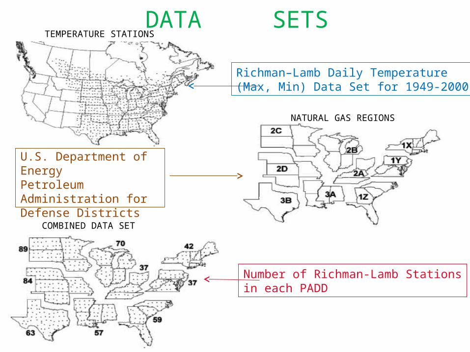
DATA SETS
Richman–Lamb Daily Temperature(Max, Min) Data Set for 1949-2000
U.S. Department of EnergyPetroleum Administration forDefense Districts (PADDs) (monthly/state data)
Number of Richman-Lamb Stationsin each PADD
TEMPERATURE STATIONS
NATURAL GAS REGIONS
COMBINED DATA SET

Fig. 4. Mean seasonal residential natural gas consumption [first number below PADD name, billions of cubic feet (Bcf)], percentage of total U.S. residential natural gas consumption (second number below PADD name), and per capita consumption [bottom number; thousands of cubic feet (Mcf)] for each PADD for (a) 3-month (December–February) winters and (b) 4-month (November–February) winters during 1989–2000. Gas data were obtained from the Energy Information Administration Internet site given in the text. PADD populations were averages of census totals for 1990 and 2000 obtained online (see http://txsdc.utsa.edu/txdata/apport/respop_b.php).
IMPORTANCE OF NATURAL GAS
Per capita consumption in 2B >> 1X despite similar latitudePer capita consumption in 2A > 1Y despite similar latitudeOther fuels are used for heating in 1X and 1Y (mountain barrier)
(a) 3-month (Dec-Feb) (b) 4-month (Nov-Feb)
2 C
2 D
3 B
3 A 1 Z
2 A
2 B
1 Y
1 X1 1 04 . 8 %1 2 . 4
1 5 86 . 9 %1 2 . 3
1 2 35 . 4 %6 . 5
5 4 22 3 . 7 %1 6 . 7
8 53 . 7 %6 . 1
2 2 81 0 . 0 %1 1 . 3
2 5 11 1 . 0 %7 . 8
3 1 71 3 . 9 %9 . 1
1 0 04 . 4 %3 . 1
2 C
2 D
3 B
3 A 1 Z
2 A
2 B
1 Y
1 X1 3 34 . 9 %1 5 . 0
1 8 46 . 8 %1 4 . 3
1 4 45 . 3 %7 . 6
6 5 62 4 . 1 %2 0 . 2
9 73 . 6 %7 . 0
2 7 41 0 . 1 %1 3 . 5
2 9 91 1 . 0 %9 . 3
3 7 51 3 . 8 %1 0 . 7
1 1 94 . 4 %3 . 6

MAXIMUM GAS CONSUMPTION-TEMPERATURE CORRELATIONS
Top = 3 month wintersBottom = 4 month winters
Monthly Seasonal
Stronger in N than SN weaker in New EnglandDBP/HDD very similar (esp. N)S weakened in Jan (esp) & Feb
N/S contrast reducedNew England contrast reducedLess effect of Jan in SInclusion of Nov also contributes

SEASONAL PREDICTION TOOLS ?Example set of regression equations -- seasonal, 3-month (Dec-Feb) winters, T-mean daily temperature index -- for DBP/HDD that gave largest correlations with natural gas consumption
Winter temperature predictive skill (ENSO-based) is highest for areas where temperature-gas consumption relations are very strong Wisconsin and Illinois (western PADD 2B), Kentucky and Tennessee (southern PADD 2A), OR moderately strong Carolinas (northern PADD 1Z),Minnesota and eastern North Dakota (eastern PADD 2C). Reverse is case for New England (PADD 1X).
“Transition to Operations” would need underpinning by statistical analyses of historical temperaturedata translate categorical NWS seasonal predictions into DBP/HDD ranges appropriate for ensemble-type prediction approach.

CONTROL OF EL NIÑO ON PRECIPITATION EL NIÑO COMPOSITE
(mm)
Monthly Anomaly
1998 EL NIÑO 2010 EL NIÑO
6 MONTH LEAD TIME
SUBSTANTIAL OPPORTUNITYfor SOCIETALRESPONSE
IS POTENTIALBEING REALIZED?
Mar 1998
STRONG PREDICTABILITY
Feb 2010
Similar to January?
Mar 2010
?
Jan 2010
ILLUSTRATION #2 WEST AFRICAN MONSOON RAINFALL
CONTROL OF INTERTROPICAL FRONT (ITF) ON RAINFALL
based on climate data set availability of impacts data sets? (e.g., malaria, meningitis)
ITF-BASED PREDICTABILITY OF RAINFALL
relation to climate system? applicability to impacts?
(from Lélé and Lamb, J. Climate, 2010)

LONG-TERM AVERAGE CLIMATOLOGY
OF ITF DISPLACEMENT (1974-2003)
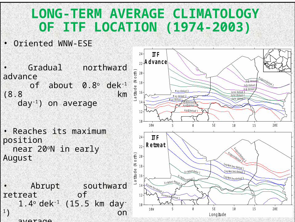
• Oriented WNW-ESE
• Gradual northward advance of about 0.8o dek-1 (8.8 km day-1) on average
• Reaches its maximum position near 20oN in early August
• Abrupt southward retreat of 1.4o dek-1 (15.5 km day-1) on average.
• Retreat almost twice as fast as advance – WHY ?
5 0 10 1510
12
14
16
18
20
22
24
Latit
ude
(Nor
th)
April dekad 2April dekad 3
M ay dekad 1M ay dekad 2
M ay dekad 3
June dekad 1June dekad 2June dekad 3
July dekad 1July dekad 2
July dekad 3
10W 5E 20E
ITFAdvance
Longitude
10
12
14
16
18
20
22
24La
titud
e (
Nor
th)
10W 5 0 5E 10 15 20E
ITFRetreat
LONG-TERM AVERAGE CLIMATOLOGYOF ITF LOCATION (1974-2003)

LONG-TERM AVERAGE ITF LOCATIONS AND RAINFALL PATTERN
10W 0 10E 20E 10W 0 10E 20E
10W 0 10E 20E 10W 0 10E 20E
ITF
JUNE
10N
15N
20N
25N
JULY
ITF
1 2 3 4 5 6 7 8 9
OCT-OBER
ITF
SEPT-EMBER
ITF
10N
15N
20N
25N10W 0 10E 20E
AUG-UST
ITF
10N
15N
20N
25N
10N
15N
20N
25N
APRIL
ITF
MAY
ITF ITF Advance = northward displacement of rainfall zones
ITF Retreat = southward displacement of rainfall zones
Peak of the rainfall season = northernmost ITF position
mm d-1
14
16
18
20
74 76 78 80 82 84 86 88 90 92 94 96 98 00 02
0
10
20
30
40
14 15 16 17 18 19 20 21
0
10
20
30
40
12
14
16
18
20
74 76 78 80 82 84 86 88 90 92 94 96 98 00 02
0
10
20
30
40
12 13 14 15 16 17 18 19 20 21
0
10
20
30
40
10
12
14
16
74 76 78 80 82 84 86 88 90 92 94 96 98 00 02
0
4
8
12
16
10 11 12 13 14
0
4
8
12
12
14
16
18
20
74 76 78 80 82 84 86 88 90 92 94 96 98 00 02
0
10
20
30
40
50
12 13 14 15 16 17 18
0
10
20
30
40
50
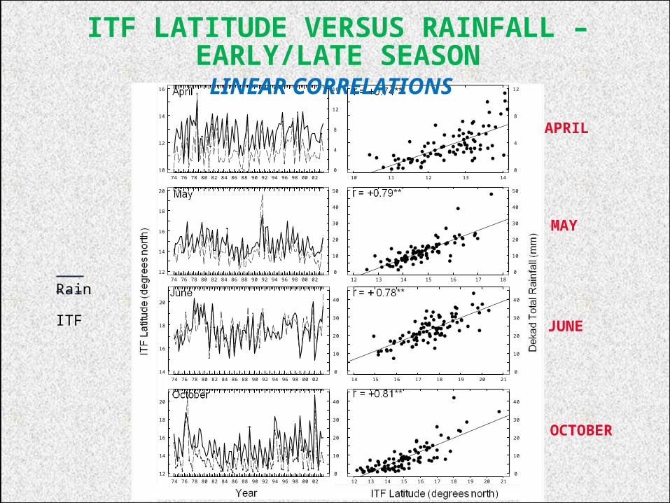
ITF LATITUDE VERSUS RAINFALL – EARLY/LATE SEASONLINEAR CORRELATIONS
Rain ITF
APRIL
MAY
JUNE
OCTOBER

ITF LATITUDE VERSUS RAINFALL -- RAINY SEASON CORELINEAR CORRELATIONS
Rain ITF
JULY
AUGUST
SEPTEMBER
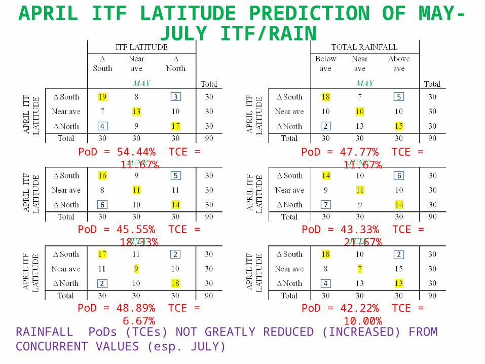
APRIL ITF LATITUDE PREDICTION OF MAY-JULY ITF/RAIN
PoD = 54.44% TCE = 11.67% PoD = 47.77% TCE = 11.67%
PoD = 45.55% TCE = 18.33% PoD = 43.33% TCE = 21.67%
PoD = 48.89% TCE = 6.67% PoD = 42.22% TCE = 10.00%
RAINFALL PoDs (TCEs) NOT GREATLY REDUCED (INCREASED) FROM CONCURRENT VALUES (esp. JULY)

APRIL ITF LATITUDE PREDICTION OF AUG-OCT ITF/ RAIN
PoD = 31.11% (38.89%) TCE = 40.00% (28.33%) PoD = 35.56% (37.77%) TCE = 36.67% (33.33%)
SEPTEMBER-OCTOBER PoDs (TCEs) ARE LARGER (SMALLER) FOR OPPOSITE DIAGONALS (EXTREME TERCILES) ….. ITF TENDS TO RETREAT SOUTH EARLY (LATE) AFTER ADVANCING NORTH EARLY (LATE)
CLIMAT-OLOGY

GENERALIZED MODELING FRAMEWORK
DECISION MODEL (often includes economics)
PROCESS MODEL
e.g., plant growth water monitoring disease transmission
REQUIRES DAILY WEATHER DATA

PROFESSIONAL DEVELOPMENT …
MUST RECOGNIZE THE NEED TO USE DAILY DATA
WMO RESOLUTION 40 (June 1995)
Members should provide to the research and education communities, for their non-commercial activities, free and unrestricted access to all data andproducts exchanged under the auspices of WMO …”
“In adopting the new policy, Congress stressed that WMO was committing itselfto broadening and enhancing the free and unrestricted international exchangeof meteorological and related data and products. The new practice states that:
Top Related