


Languages
Pages
Legal

Probability&
Standard Error of the Mean

Definition Review Population: all possible cases
Parameters describe the population Sample: subset of cases drawn from
the population Statistics describe the sample
Statistics = Parameters

Why Sample????
Can afford it

Can afford it Can do it in reasonable time
Why Sample????
Can afford it Can do it in reasonable time Can estimate the amount of error
(uncertainty) in statistics, allowing us to generalize (within limits) to our population
Why Sample????

Even with True Random Selection
Some error (inaccuracy) associated with the statistics (will not precisely match the parameters) sampling error: everybody is different
The whole measured only if ALL the parts are measured.

With unbiased sampling
Know that the amount of error is reduced as the n is increased statistics more closely approximate the
parameters Amount of error associated with
statistics can be evaluated estimate by how much our statistics may
differ from the parameters

Sample size Rules of thumb
Larger n the better law of diminishing returns
ie 100 to 200 vs 1500 to 1600 $$$ and time constraints
Less variability in population => better estimate in statistics reduce factors affecting variability
control and standardization

Human beingsare
terriblerandomizers
True Random sampling: rare
What population is the investigator interested in???
Getting a true random sample of any population is difficult if not impossible subject refusal to participate

Catch 22NEVER know our true
population parameters, so we are ALWAYS at risk of making an error in generalization

Probability

Probability: the number of times some event is likely to occur out of the total possible events
p =# particular event
# of possible events
Backbone of inferential stats

The classic: flip a coin heads vs tails: each at 1/2 (50%) flip 8x: what possible events (outcomes)?? flip it 8 million times: what probable
distribution of heads/tails?
Backbone of inferential stats

Wayne Gretzky

Wayne Gretzky & probability
What is the probability that a geeky looking kid from Brantford, Ontario, Canada would meet, much less marry, a movie star?

Wayne’s famous quote:

Wayne Gretzky redux.

Life with Probability
life insurance rates obesity smoking
car insurance rates age previous accidents driving demerits
flood insurance All
life
dep
ends
on
prob
abil
itie
sV
olta
ire
(175
6)

The Ever-Changing Nature of %s
Never go for a 50-50 ball unless you're 80-20 sure of winning it.
Ian Darke
The 50/50/90 Rule: whenever you have a 50/50 chance of guessing at something,
there’s a 90% chance you will guess wrong. Menard’s Philosophy

How to Count Cards
We are going to show you how to count cards. Card counting is not illegal. If caught counting cards you will not be arrested. You will not be taken into the back room and beaten unconscious, then dragged to the desert and buried with the rest of the casino cheaters. You will not get your fingers cut off with a butcher knife by Michael Corleone. However, if caught counting cards you may be banned from playing at that casino. You have to be smart about counting cards and don't be too obvious. You do not want to be banned from the casino that you are sleeping at. If you are going to try your luck at counting cards we suggest you go down the street to a different casino in case you get caught. Use this information at your own risk.
From [email protected]

One of the most popular card counting systems currently in use is the point count system, also known as Hi-Low. This system is based on assigning a point value of +1, 0, or -1 to every card dealt to all players on the table, including the dealer. Each card is assigned its own specific point value. Aces and 10-point cards are assigned a value of -1. Cards 7, 8, 9 each count as 0. Cards 2, 3, 4, 5, and 6 each count as +1. As the cards are dealt, the player mentally keeps a running count of the cards exposed, and makes wagering decisions based on the current count total.

•The higher the plus count, i.e. the higher percentage of ten-point cards and aces remaining to be dealt, means that the advantage is to player and he/she should increase their wager.
•If the running count is around zero, the deck or shoe is neutral and neither the player nor the dealer has an advantage.
• The higher the minus count, the greater disadvantage it is to the player, as a higher than normal number of 'stiff' cards remains to be dealt. In this case a player should be making their minimum wager or leave the table.

As the dealing of the cards progresses, the credibility of the count becomes more accurate, and the size of the player's wager can be increased or decreased with a better probability of winning when the deck or shoe is rich in face cards and aces, and betting and losing less when the deck is rich in 'stiff' cards. It is important to note that a player's decision process, when to hit, stand, double down, etc. is still based on basic strategy. Remember, you MUST learn basic strategy. However, alterations in basic strategy play is sometimes recommended based on the current card count.
For example, if the running count is +2 or greater and you have a hard 16 against a dealer's up card of ten, you should stand, which is a direct violation of basic strategy. But considering that the deck or shoe is rich in face cards you are more likely to bust in this situation, thus you ignore basic strategy and stand. Another example is to always take insurance when the count is +3 or greater. For the most part however, you should stick with basic strategy and use the card count as an indication of when to increase or decrease the amount of your bet, as that is the whole strategy behind card counting.

Probability & the Normal Curve Normal Curve
mathematical abstraction unimodal symmetrical (Mean = Mode = Md) Asymptotic (any score possible) a family of curves
Means the same, SDs are different Means are different, SDs the same both Means & SDs are different

Each dice has six equal possible outcomes when thrown - numbers one through six.
The two dice thrown together have a total of 36 possible outcomes, the six combinations of one dice by the six combination of the other.
Dice Roll Outcomes

Numbers Combinations Dice Combinations2 one 1 13 two 1 2, 2 14 three 1 3, 3 1, 2 25 four 1 4, 4 1, 2 3, 3 26 five 1 5, 5 1, 2 4, 4 2, 3 37 six 1 6, 6 1, 2 5, 5 2, 3 4, 4 38 five 2 6, 6 2, 3 5, 5 3, 4 49 four 3 6, 6 3, 4 5, 5 410 three 4 6, 6 4, 5 511 two 5 6, 6 512 one 6 6
Dice Roll Outcomes
Notice how certain totals have more possibilities of being thrown, or are more probable of occurring by random throw of the two dice.
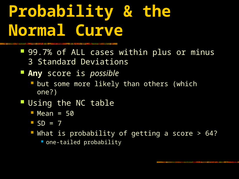
99.7% of ALL cases within plus or minus 3 Standard Deviations
Any score is possible but some more likely than others (which one?)
Using the NC table Mean = 50 SD = 7 What is probability of getting a score > 64?
one-tailed probability
Probability & the Normal Curve
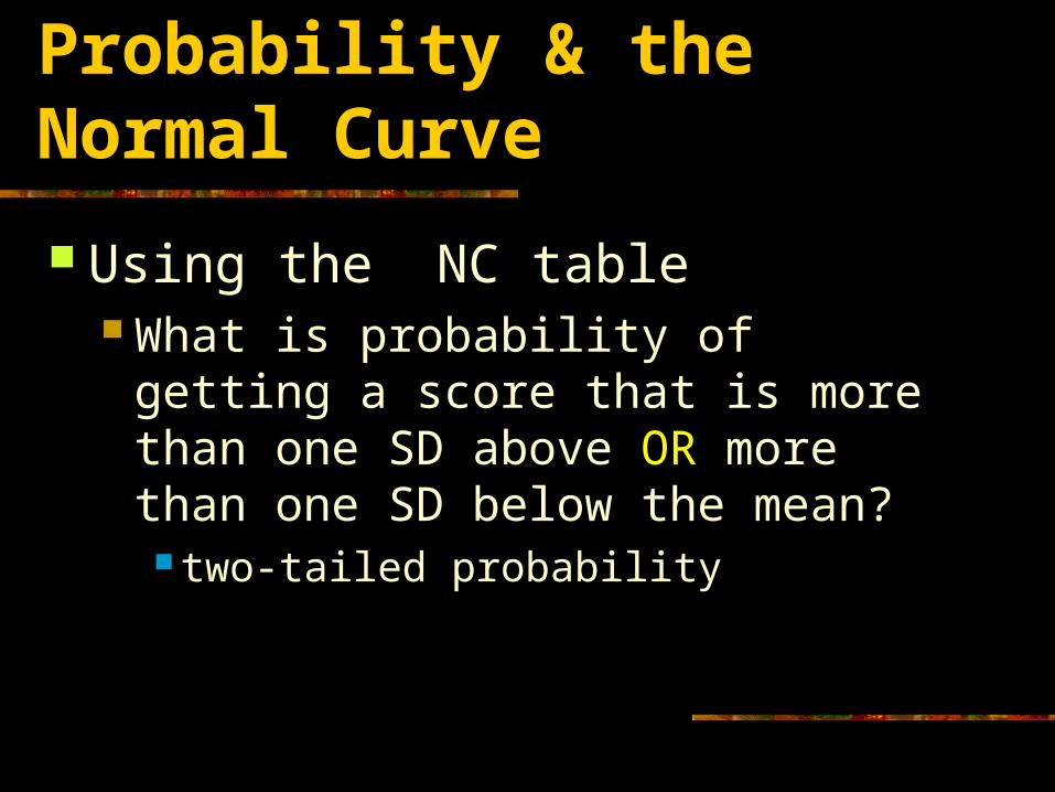
Using the NC table What is probability of getting a score
that is more than one SD above OR more than one SD below the mean?
two-tailed probability
Probability & the Normal Curve

Defining probable or likely
What risk are YOU willing to take? Fly to Europe for $1,000,000 BUT…
50% chance plane will crash 25% chance 1%chance .001% chance .000000001% chance

Defining probable or likely
In science, we accept as unlikely to have occurred at random (by chance) 5% (0.05) 1% (0.01) 10% (0.10)
May beone-tailedor two-tailed

Serious people takeseriously probabilities, not mere possibilities.
George Will, 11/2/2000

Six monkeys fail to write Shakespeare
Pantagraph, May 2003

Any score is possible, but some more likely than others
Key to any problem in statistical inference is to discover what sample values will occur in repeated sampling and with what probability.
With what probability will a score arise by chance that is as extreme
as a certain value????
Probability & the Normal Curve

Statistics HumourA man who travels a lot was concerned about the possibility of a bomb on boardhis plane. He determined the probability of this, found it to be low but not lowenough for him. So now he always travels with a bomb in his suitcase. He reasonsthat the probability of two bombs beingon board would be infinitesimal.

Sampling Distributions:
Standard error of the mean

Recall With sampling, we EXPECT error in
our statistics statistics not equal to parameters
cause: random (chance) errors

Recall With sampling, we EXPECT error in
our statistics statistics not equal to parameters
cause: random (chance) errors
Unbiased sampling: no factor(s) systematically pushing estimate in a particular direction

Recall With sampling, we EXPECT error in our
statistics statistics not equal to parameters
cause: random (chance) errors
Unbiased sampling: no factors systematically pushing estimate in a particular direction
Larger sample = less error

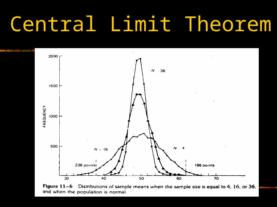
Central Limit Theorem
Consider (conceptualize) a distribution of sample means drawn from a distribution repeated sampling (calculating mean) from
the same population produces a distribution of sample means

Central Limit Theorem
A distribution of sample means drawn from a distribution (the sampling distribution of means) will be a normal distribution
class: from list of 51 state taxes, each student create 5 random samples of n = 6. Look at distribution in SPSS
Mp = 32.7 cents, SD = 18.1 cents

Central Limit Theorem
Mean of distribution of sampling means equals population mean if the n of means is large

Central Limit Theorem
Mean of distribution of sampling means equals population mean if the n of means is large true even when population is skewed if
sample is large (n > 60)

Central Limit Theorem Mean of distribution of sampling means
equals population mean if the n of means is large true if population when skewed if sample is
large (n > 60) SD of the distribution of sampling
means is the Standard Error of the Mean
Take home lesson We have quantified the expected error
(estimate of uncertainty) associated with our sample mean Standard Error of the Mean
SD of the distribution of sampling means

Typical procedure Sample
calculate mean & SD

Typical procedure Sample
calculate mean & SD KNOW & RECOGNIZE that

Typical procedure Sample
calculate mean & SD KNOW & RECOGNIZE that
statistics are not exact estimates of parameters

Typical procedure
Sample calculate mean & SD
KNOW & RECOGNIZE that statistics are not exact estimates of
parameters a larger n provides a less variable measure of
the mean
Central Limit Theorem

Typical procedure
Sample, calculate mean & SD KNOW & RECOGNIZE that
statistics are not exact estimates of the parameters
a larger n provides a less variable measure of the mean
sampling from a population with low variability gives a more precise estimate of the mean
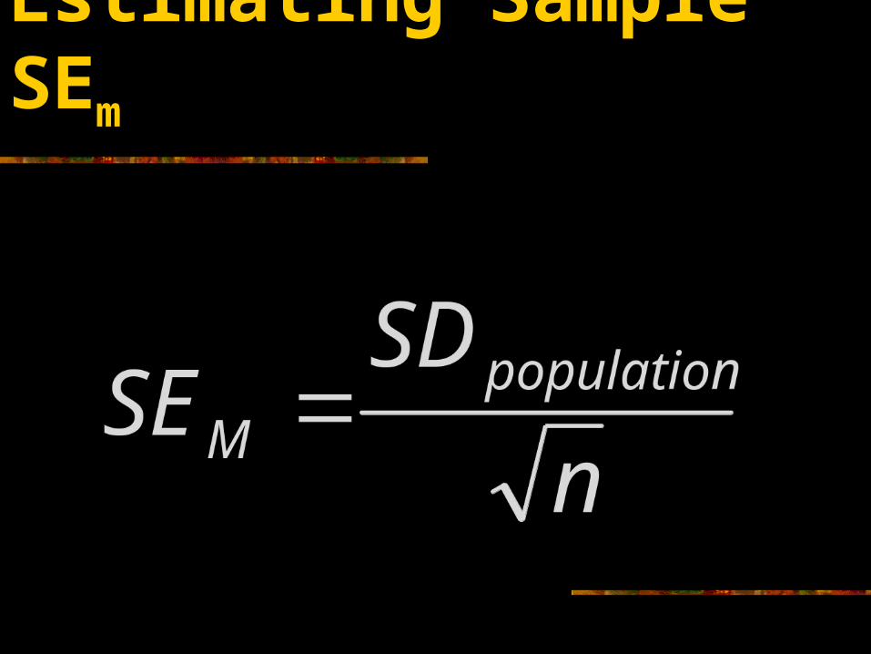
Estimating Sample SEm

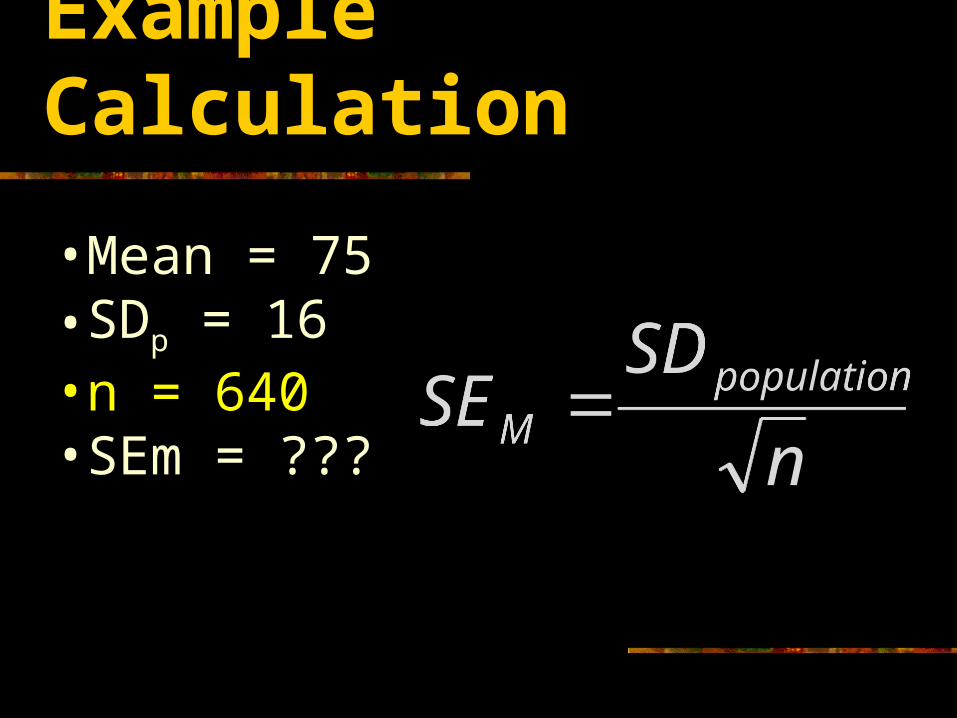
Example Calculation
•Mean = 75•SDp = 16•n = 64•SEm = ???

Confidence Interval for the Mean
•Mean = 75•SDp = 16•n = 64 •SEm = 2
68%
Distribution ofsampling means

•Mean = 75•SDp = 16•n = 64 •SEm = 2
68%
We are about 68% sure thatpopulation meanlies between 73and 77
7573 77
Samplemean
Confidence Interval for the Mean

•Mean = 75•SDp = 16•n = 64 •SEm = 2
68%
7573 77
Samplemean
73 and 77 are theupper and lowerlimits of the 68%confidence intervalfor the population mean
Confidence Interval for the Mean

Example Calculation
•Mean = 75•SDp = 16 •n = 16•SEm = ???
Example Calculation
•Mean = 75•SDp = 16 •n = 640•SEm = ???

Example Calculation
•Mean = 75•SDp = 160 •n = 16•SEm = ???

Example Calculation
•Mean = 75•SDp = 160 •n = 640•SEm = ???

Explain how SD and n affect the error inherent
in estimating the population mean
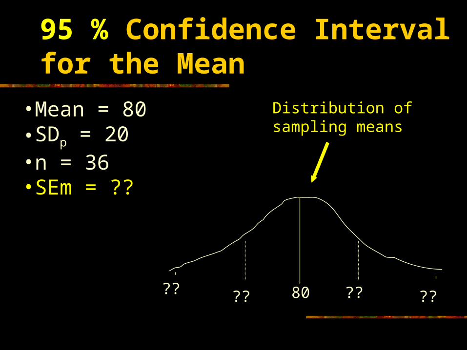
95 % Confidence Interval for the Mean
•Mean = 80•SDp = 20•n = 36 •SEm = ??
80?? ???? ??
Distribution ofsampling means

•Mean = 80•SDp = 20•n = 36 •SEm = 3.33
95%
8076.67 83.3373.34 86.66
1.96 * 3.33 = 6.53Up = 80 + 6.53Lo = 80 - 6.53
SEMXLimits 96.1
95 % Confidence Interval for the Mean

•Mean = 80•SDp = 20•n = 36 •SEm = 3.33
95%
73.47 and 86.53 are theupper and lowerlimits of the 95%confidence intervalfor the population mean
Samplemean
8076.67 83.3373.34 86.66
73.47 86.53
95 % Confidence Interval for the Mean

Key to any problem in statisticalinference is to discover what sample values will occur inrepeated sampling and with what probability.
Top Related