


Languages
Pages
Legal


1
Private Information in the Chinese Stock Market:
Evidence from Mutual Funds and Corporate Insiders*
Yeguang Chi†
October 1, 2014
ABSTRACT
I find evidence of valuable private information in the Chinese stock market. First, I
find that Chinese actively managed stock mutual funds outperform passive
benchmarks including market, size, value-growth, and momentum factors. Most
funds appear to have skill, and much of that skill consists of stock-picking ability.
Second, Chinese corporate insiders also outperform the market. Moreover, the
performance of stock funds is positively correlated with the performance of
corporate insiders. Funds that trade more in correlation with insiders perform better.
Funds’ larger share positions correlate more with insiders. Funds with a higher
portfolio concentration in these large positions outperform funds with a lower
concentration. Finally, I find evidence of stock funds’ performance erosion, a sign of
improvement in market efficiency.
* I thank Professor Lubos Pastor for valuable advice and guidance. I also thank Professors Eugene Fama, Lars Hansen, Bryan Kelly, and Juhani Linnainmaa, and seminar participants at the Booth Brownbag Workshop for their feedback and comments. I acknowledge financial support from the John and Serena Liew Fellowship Fund at the Fama-Miller Center for Research in Finance, the University of Chicago Booth School of Business. All errors are mine. † The University of Chicago Booth School of Business and Economics Department, Email:

2
“The China Securities Regulatory Commission has opened 25 insider trading investigations
since the start of the year, up from 22 for all of 2013, and has referred 29 cases to police and
prosecutors, up from 21 in 2013…At least 178 fund managers have left their jobs in the first six
months of this year, compared with 150 in all of 2013…The large number of fund managers
leaving this year has a direct relationship with the probes…Insider trading is seen as common
on China’s domestic bourses.”
Financial Times, July 7, 2014
The primary role of a financial market is to allocate the economy’s capital stock. To do so
efficiently, the market must rely on prices that provide accurate signals for resource allocation.
Fama (1965, 1970) defines an efficient market as a market in which prices always fully reflect
available information. Strong-form efficiency concerns whether given investors have
monopolistic access to any information relevant to price formation. Subsequent studies on
insider trading such as Jaffe (1974), Finnerty (1976), Seyhun (1986) and Lakonishok and Lee
(2001), have presented evidence that suggests violation of strong-form efficiency in the U.S.
stock market. Corporate insiders in the U.S. seem to possess private information that helps them
generate trading profits. Semi-strong form efficiency concerns whether prices efficiently adjust
to publicly available information. Performance evaluation of U.S. mutual fund managers has lent
support to this hypothesis. Fama and French (2010) show that, in aggregate, actively managed
U.S. stock mutual funds do not beat the market, and very few funds produce benchmark-adjusted
returns sufficient to cover their costs.
Thus, the extent to which private information is exploited in the U.S. stock market seems
limited. That so few professional fund managers can beat the market suggests the U.S. stock
market is not grossly inefficient in semi-strong form. A well-developed legal system and harsh
punishment for insider trading have contributed to this efficiency.1 The U.S. stock market is
probably the most efficient marketplace in the world. An interesting question then is to ask how
private information is exploited in a less developed financial market. China is a natural candidate
for such investigation.
Established in 1990, the Chinese stock market has a short history, but it has seen tremendous
growth. As of 2012, it surpassed Japan to become the second largest stock market in the world.
Meanwhile, financial laws and regulations have been introduced gradually to address new
developments in the Chinese financial markets. However, as is common in emerging markets,
the legal system in China is not as fully developed as that in the United States. For example,
regulations on insider trading were introduced only recently, in April 2007. Meanwhile, Chinese
retail investors represent a large fraction of the stock market. In 2003, they held over 87% of the
total stock market capitalization. With a shorter history, a weaker legal system, and a significant
presence of retail investors, the emerging Chinese stock market provides an excellent target for
this study.
1 For example, in 2011, Galleon Group hedge fund founder Raj Rajaratnam was sentenced in New York to 11 years for illegal trading on inside information. He was ordered to pay a $10 million fine and forfeit $53.8 million. In 2014, Mathew Martoma, a former portfolio manager at SAC Capital Advisors LP hedge fund, was sentenced to 9 years in prison for illegal trading on inside information. He was ordered to forfeit $9.3 million, including his Boca Raton, Florida, home.
3
In this paper, I focus on two groups of investors in China: actively managed stock mutual
funds and corporate insiders. Actively managed stock mutual funds represent a substantial
portion of the Chinese stock market in terms of both assets under management and stock market
coverage. For example, in 2007, their aggregate holdings represented 16.6% of the Chinese stock
market capitalization. Chinese corporate insiders trade a substantial amount of their own
company stocks. From April 2007 to June 2014, their total trading volume amounted to nearly
RMB900 billion, which represents about 0.3% of the total trading volume in the market.2
The first part of my analysis focuses on the performance evaluation of Chinese actively
managed stock mutual funds. I find that despite representing a substantial share of the Chinese
stock market, the aggregate portfolio of Chinese actively managed stock mutual funds
outperforms passive benchmarks including market, size, value-growth, and momentum factors.
First, I show results based on the aggregate portfolio of actively managed stock funds. Second, I
perform bootstrap simulations based on a zero-α return sample and find that most managers have
sufficient skill to cover all costs. Finally, I investigate their semiannual stock holdings and find
evidence of stock-picking skills that help explain a substantial amount of the funds’ α.
These findings are in sharp contrast to Fama and French (2010)’s result on U.S. stock mutual
funds. They conclude the aggregate portfolio of actively managed U.S. stock funds is very close
to the stock market portfolio, and few funds produce benchmark-adjusted returns sufficient to
cover their costs. Therefore, the evidence of Chinese fund managers’ outperformance suggests
that either they are good at interpreting public information, or they are able to exploit private
information. The former explanation is at least partly true, because professional fund managers
presumably have better knowledge and skill than an average market participant. Attributing
some of their outperformance to their skill at interpreting public information is reasonable. The
more relevant question for my study is the latter explanation, that is, to what extent are the fund
managers exploiting private information?
To answer this question, I first study the trading activity of Chinese corporate insiders, the
group of investors that intrinsically have access to private information about their own company.
I discover strong evidence of information asymmetry in the Chinese stock market. Chinese
corporate insiders are able to generate abnormal profits by trading their own company stocks.
Stocks insiders buy tend to do well. Stocks insiders sell tend to do poorly. The positive return
associated with insider buys is strong and lasts for at least 12 months after the insider trades. The
negative return associated with insider sells is strong in the short term (one month) but quickly
decays afterward. This finding is consistent with the intuition that insider sells may be motivated
by reasons other than negative private information, such as liquidity and diversification needs.
Insider buys, on the other hand, are much more likely driven by positive private information with
a more permanent impact on returns. This result is economically significant. A simple insider-
mimicking trading strategy produces a significantly positive annual alpha of 14.43% (t=3.08)
against the market benchmark.
2 RMB is the official currency of China. The RMB/USD exchange rate prior to July 2005 is pegged at 8.28RMB/USD. Since then, RMB has appreciated to 6.16RMB/USD by mid 2014. All numerical values presented in this paper are in RMB unless otherwise specified.

4
Having established that Chinese corporate insiders possess valuable private information, I then
turn to the investigation of possible connections between the performance of corporate insiders
and stock funds. I find evidence that points to some intersection between these two groups’
information sets. First, I show a strong correlation between the return series of stock funds’
trading portfolio and the insider-mimicking trading portfolio. Second, I find that funds that trade
more in correlation with insiders deliver better performance. Next, I define a stock fund’s
qualified holdings as those stock holdings that represent a large fraction of the stocks’ market
capitalization. In other words, a fund’s qualified stock holdings represent a significant share
percentage of the corresponding stocks. I show a significant correlation between the insider-
mimicking portfolio and the aggregate qualified-holding portfolio. Furthermore, I use a fund’s
concentration in these qualified holdings as a proxy for the fund’s access to inside information. I
find funds with a higher concentration in these qualified holdings outperform funds with a lower
concentration.
Last but not least, I present evidence of performance erosion in Chinese stock mutual funds.
There is a significantly negative time trend in stock funds’ aggregate performance. These results
are consistent with the Chinese stock market becoming more efficient and harder to beat. It is
also consistent with the fact that more institutional presence in the Chinese stock market
introduces more competition. The retail fraction of the Chinese stock market decreased from 87%
in 2003 to 36% in 2013. Of course, the decline in the retail fraction coincides with the rise of the
institutional fraction. The institutionally managed fraction of the Chinese stock market has
grown from 13% to 64% in just 10 years.3
This paper contributes to several strands of the finance literature. First, it adds to the literature
on mutual fund performance evaluation. Since Jensen’s 1968 study on U.S. mutual funds’
performance from 1945 to 1964, many papers in this literature have attempted to get a better
understanding and more accurate assessment of their performance (e.g. Grinblatt and Titman
(1989), Carhart (1997), Chen, Jegadeesh and Wermers (2000), Wermers (1999,2000), Pastor and
Stambaugh (2002), Berk and Green (2004), Cohen, Coval and Pastor (2005), Busse and Irvine
(2006), Fama and French (2010), Pastor and Stambaugh (2012), Linnainmaa (2013), Pastor,
Stambaugh and Taylor (2014)). However, the U.S. literature has given no attention to the
Chinese mutual fund industry, partly due to its short history and partly due to the lack of data.
The finance literature in China has some coverage of mutual fund performance, but with very
limited data. For example, Su et al. (2012) had a sample of only 42 funds. Wang (2011) had a
sample period of only four years. Earlier works such as Li, Chen and Mao (2007) and Luo, Wang
and Tian (2003) had even smaller sample sizes. In this paper I construct and study a
comprehensive data set since the inception of the Chinese stock mutual fund industry. My data
set covers 418 Chinese actively managed stock mutual funds for a sample period of over 16
years.
Fama and French (2010) show that U.S. actively managed stock mutual funds do not
outperform the market. Only the managers in the right tail of the distribution seem to possess
3 Pastor, Stambaugh, and Taylor (2014) find similar evidence of rising competition in the U.S. stock market. They find that the rising competition is offset by the rising skill of active mutual funds, so that the net effect on the performance of U.S. active funds is approximately neutral. In contrast, I find that competition in China has risen so fast that the performance of Chinese funds has declined over time.

5
skill that help them generate positive α. By contrast, I find widespread skill among Chinese
mutual funds. I present strong evidence of outperformance, both in aggregate fund returns
through a regression framework, and in individual fund returns through a bootstrap simulation
approach. Furthermore, I show managers possess stock-picking abilities that help them generate
a positive α. Using the methodology advocated by Berk and Binsbergen (2014), I find the
aggregate outperformance of Chinese stock mutual funds amounted to over RMB233 billion (in
Y2010 RMB), for a period from July 2003 to June 2014.
Second, this paper adds to the literature on the informational efficiency of financial markets.
Fama (1965, 1970) introduced the efficient-market hypothesis. Subsequent studies on insider
trading, such as Jaffe (1974), Finnerty (1976), Seyhun (1986), and Lakonishok and Lee (2001),
have presented evidence that suggests violation of strong-form efficiency in the U.S. stock
market. In this paper, I assemble and study a novel data set on the Chinese corporate insiders’
trading activities. I add empirical evidence to this literature in the context of the Chinese stock
market. I find that stocks bought by insiders tend to increase in value subsequently, whereas
stocks sold by insiders tend to lose value. Chinese corporate insiders seem to possess private
information that helps them generate trading profit to beat the market. In addition, I find the
positive return associated with insider buys tends to be more permanent than the negative return
associated with insider sells. This finding confirms the intuition that reasons other than negative
private information, such as liquidity and diversification needs, may motivate insider sells.
Insider buys, on the other hand, are much more likely driven by positive private information.
Third, this paper adds to the literature on mutual fund performance attribution. Papers in this
literature try to understand channels from which mutual fund managers derive their
outperformance. Treynor and Mazuy (1966) and Henriksson and Merton (1984) design
regression frameworks to test for managers’ market-timing skills. Daniel et al. (1997) construct
characteristic-based benchmarks to capture manager skill in stock picking and characteristic
timing. Kacperczyk, Sialm, and Zheng (2005) offer evidence of manager skill by showing that
funds with higher industry concentration outperform. Cohen, Coval, and Pastor (2005) find a
relationship between stock quality and manager skill and design a new performance measure
incorporating a fund’s stock holdings’ qualities. Kacperczyk and Seru (2007) focus on the
manager-skill channel that depends on the degree to which a fund manager relies on public
information. In my paper, I first show that a substantial amount of manager skill can be attributed
to stock-picking ability. In addition, I establish a strong correlation between stock mutual funds
and corporate insiders in China. By studying both groups’ return series and trading activities, I
discover a significant correlation between the performance of the aggregate stock fund portfolio
and the insider-mimicking portfolio. Cross-sectionally, funds that trade in more correlation with
insiders tend to outperform those that trade in less correlation with insiders. Lastly, mutual funds’
qualified holdings (large share positions measured by the stock holding’s value divided by the
stock’s market capitalization) show a significantly positive return correlation with the insider-
mimicking portfolio. Funds more concentrated in such holdings outperform those less
concentrated in such holdings. All evidence is consistent with the intuition that Chinese stock
fund managers may be exploiting similar private information that insiders possess.
Finally, this paper also contributes to the understanding of Sharpe’s (1991) arithmetic of active
investing in the context of the Chinese stock market. I study two novel data sets of Chinese stock
mutual funds and corporate insiders. I find they both outperform the market. Retail investors in

6
China account for over 87% of the stock market capitalization in 2003. Most of these retail
investors actively manage their portfolios, because passive money management captures little of
the Chinese stock market capitalization. This market environment aids professional stock fund
managers in their pursuit to beat the market at the expense of retail investors. Barber et al. (2012)
document similar evidence from Taiwanese individual day traders. They find that less than 1%
of the total population of day traders is able to predictably and reliably earn positive abnormal
returns net of fees. Odean (1999) and Barber and Odean (2000) document evidence of excessive
trading among U.S. retail investors. They conclude that these investors pay a tremendous
performance penalty for active trading. I find similar results that Chinese retail investors in
aggregate underperform common passive benchmarks. This observation is not surprising, given
that institutional investors are equipped with better financial knowledge and a vaster amount of
resources, not to mention their access to potential private information. As a consequence,
Chinese retail investors are paying a tremendous performance penalty for active trading.
The closest paper to mine is a contemporaneous paper by Choi, Jin, and Yan (2014), which
studies Chinese stock ownership data from 1996 to 2007. They show that Chinese institutional
investors have a strong information advantage, and past aggressiveness of institutional trading in
a stock positively predicts institutions’ future information advantage in this stock. While my
focus is similar, my data and empirical methodology are very different from those used by Choi,
Jin, and Yan (2014). Specifically, I analyze stock mutual funds (1998-2014) and corporate
insiders (2007-2014). Choi, Jin, and Yan (2014) find evidence of institutional investors’
outperformance, which is consistent with and complementary to my results on stock funds and
corporate insiders. In addition to the outperformance results, I investigate the correlation patterns
between stock funds and corporate insiders. I find evidence that points to some intersection
between these two groups of active investors’ information sets. Moreover, I study the
performance erosion of stock funds in relation to the growth of institutional money-management
industry in China.
The rest of the paper is organized as follows. Section I offers background information on the
Chinese stock market and mutual funds. Section II describes the data. Section III evaluates the
performance of Chinese actively managed stock mutual funds in three different ways: (1)
aggregate return analysis, (2) bootstrap simulation analysis, and (3) holdings analysis. Section IV
evaluates the performance of Chinese corporate insider trading and constructs an insider-
mimicking portfolio. Section V investigates correlation patterns between stock funds and
corporate insiders, in connection with fund performance. Section VI shows evidence of
performance erosion for stock mutual funds. Section VII concludes. The appendix includes
additional results.
I. Chinese Stock Market and Mutual Funds
Since the inception of the first stock mutual fund in China in 1998, the growth of the Chinese
stock mutual fund industry has been steady and robust. As Table 1 shows, total assets under
management (AUM) of actively managed stock mutual funds grew from RMB2 billion in 1998 to over RMB750 billion in 2013 (for the rest of my paper, I use stock mutual funds or stock
funds interchangeably with actively managed stock mutual funds). At its peak in 2007, aggregate

7
stock fund AUM passed RMB1.5 trillion. As the number of funds reflects, Chinese stock mutual
funds have been growing steadily since 1998. As of December 2013, the Chinese stock mutual
fund industry had 380 actively managed funds. Meanwhile, the Chinese stock market has been
growing at a fast pace. In 2012, China surpassed Japan to become the second largest market as
measured by aggregate market capitalization.
Table 1 shows summary statistics of Chinese stock mutual funds and the Chinese stock market.
The ratio between stock funds’ aggregate AUM to the total stock market capitalization exceeded
16% in 2007. In the 2008 bear market, the aggregate AUM of actively managed stock mutual
funds experienced a sharp downturn, from RMB1515 billion to RMB636 billion. Since then it
bounced back to around RMB750 billion. Meanwhile, the Chinese stock market capitalization
has grown steadily. The growth in the total stock market capitalization in China is partly due to
the share-reform policy initiated in 2006. The policy is designed to convert the previously
restricted shares (mostly owned by state and local governments) into floating/tradable shares in
the secondary market. My measure of the market capitalization is based on the outstanding
shares in the secondary market. As a result, this restricted-to-floating share conversion has led to
an increasing trend in the aggregate stock market capitalization. Aggregate AUM of actively
managed stock mutual funds has been lagging the growth of the total stock market, which is why
we observe a decreasing trend in stock mutual funds’ share of the total market capitalization
since 2006. Nonetheless, as of December 2013, this ratio remained substantial at 3.8% of the
Chinese stock market capitalization. In aggregate, these funds still manage over RMB750bn. The
last three columns of Table 1 show an increasing trend in the number and percentage of stocks in
which the stock mutual funds invest. In 2003, stock funds held 515 stocks or 42.0% of all
publicly listed Chinese stocks in their portfolios. By 2013, this number increased to 1,885 or 76.4%
of all publicly listed Chinese stocks.
Clearly, actively managed stock mutual funds represent a substantial portion of the Chinese
stock market, both in terms of assets under management and stock market coverage. They
represent an even more substantial portion of the Chinese institutional investors. This is because
Chinese retail investors represent a large fraction of the stock market. In 2003, they held over 87%
of the total stock market capitalization. The retail fraction steadily decreased to 36% by the end
of 2013. That is, the institutional investors hold 64% of the stock market capitalization. Among
the institutionally managed stock market assets, actively managed stock mutual funds count for
5.7% in 2013. Data availability is the primary reason I focus on the stock funds for this study.
Because they represent a substantial portion of the institutional investors, results on stock funds
should also shed light on the performance of other types of institutional investors. In fact, I also
investigate the aggregate institutional investors’ stock holdings data and find similar results to
the holdings of stock funds.

8
Table 1
Summary Statistics on the Chinese Actively Managed Stock Mutual Funds
and the Chinese Stock Market I report number of funds, total fund AUM, aggregate stock market capitalization (Aggr. Stock MktCap), and the
ratio (AUM/MktCap) of the two in %. I report fund holdings summary statistics in the last three columns. These data
start in 2003. I report total number of stocks held by stock mutual funds in aggregate (# of Stocks held by MF), total
number of listed stocks on the exchange (# of Stocks Total), and the ratio of the two (MF/Total) in %. The data
cover 418 funds from July 1998 to December 2013. AUM and MktCap are in RMB billion.
Reporting Period
# of Funds
AUM of Funds (bn)
Aggr. Stock MktCap
(bn)
AUM / MktCap
# of Stocks held by
MF
# of Stocks Total
MF/Total
2Q/1998 1 ¥2 ¥594 0.3% 784
4Q/1998 1 ¥2 ¥557 0.4% 826
2Q/1999 7 ¥21 ¥884 2.4% 873
4Q/1999 13 ¥34 ¥800 4.2% 923
2Q/2000 17 ¥45 ¥1,289 3.5% 973
4Q/2000 20 ¥51 ¥1,564 3.3% 1,060
2Q/2001 22 ¥42 ¥1,750 2.4% 1,113
4Q/2001 33 ¥46 ¥1,344 3.4% 1,137
2Q/2002 37 ¥56 ¥1,470 3.8% 1,164
4Q/2002 39 ¥51 ¥1,182 4.3% 1,201
2Q/2003 43 ¥58 ¥1,281 4.5% 515 1,227 42.0%
4Q/2003 44 ¥63 ¥1,244 5.1% 495 1,264 39.2%
2Q/2004 45 ¥63 ¥1,204 5.2% 1,176 1,323 88.9%
4Q/2004 47 ¥66 ¥1,116 5.9% 1,202 1,354 88.8%
2Q/2005 53 ¥67 ¥953 7.1% 1,210 1,368 88.5%
4Q/2005 68 ¥88 ¥1,020 8.7% 1,210 1,356 89.2%
2Q/2006 79 ¥150 ¥1,619 9.3% 1,162 1,354 85.8%
4Q/2006 105 ¥377 ¥2,412 15.6% 1,220 1,416 86.2%
2Q/2007 116 ¥813 ¥5,413 15.0% 885 1,460 60.6%
4Q/2007 125 ¥1,515 ¥9,140 16.6% 947 1,533 61.8%
2Q/2008 140 ¥873 ¥5,919 14.7% 955 1,591 60.0%
4Q/2008 157 ¥636 ¥4,538 14.0% 932 1,609 57.9%
2Q/2009 179 ¥953 ¥9,084 10.5% 1,016 1,607 63.2%
4Q/2009 202 ¥1,049 ¥15,074 7.0% 1,305 1,702 76.7%
2Q/2010 229 ¥846 ¥12,668 6.7% 1,515 1,875 80.8%
4Q/2010 254 ¥989 ¥19,232 5.1% 1,649 2,046 80.6%
2Q/2011 279 ¥902 ¥20,051 4.5% 1,751 2,211 79.2%
4Q/2011 307 ¥747 ¥16,517 4.5% 2,053 2,323 88.4%
2Q/2012 335 ¥749 ¥17,337 4.3% 2,119 2,424 87.4%
4Q/2012 354 ¥739 ¥18,220 4.1% 1,887 2,473 76.3%
2Q/2013 369 ¥724 ¥16,979 4.3% 1,859 2,470 75.3%
4Q/2013 380 ¥758 ¥20,039 3.8% 1,885 2,467 76.4%

9
II. Data Description
Thanks to the data provider Wind Information® (WIND hereafter), a leading Chinese
financial data provider, I am able to construct several novel data sets on the Chinese financial
market. Founded in 1994, WIND serves more than 90% of the financial enterprises in the
Chinese market, including securities firms, fund management firms, insurance companies and
banks. Overseas, WIND serves 75% of the Qualified Foreign Institutional Investors (QFII).
Additionally, most renowned financial research institutions and regulatory committees are on
WIND client list. Media reporters and academic researchers frequently quote WIND data. The
other commonly used source for Chinese financial data is CSMAR on WRDS. In comparison,
WIND offers more detailed and up-to-date data on stocks and mutual funds. Moreover, WIND
collects data on Chinese insider trading activities and institutional stock holdings, which
CSMAR does not provide. For this paper, I construct four data sets covering the following parts
of the Chinese financial market: stock market, mutual funds, corporate insiders, and institutional
investors. I will discuss each of the four data sets below.
1. Chinese Stock Market Data Set
For this study, I focus on the Chinese A-share stock market, which comprises 2,555 stocks as
of June 2013. The stock mutual funds in my sample can only invest their stock portfolio in the
A-share stocks. In particular, I construct daily and monthly series for each stock’s price, holding
period return and market capitalization. Data on delisted stocks are also appropriately recorded
for the time period they existed. But overall, few stocks are delisted.
I further construct the benchmark returns from the stock market data. In particular, I calculate
the excess value-weighted market return , Fama-French factor returns SMB and HML,
as well as the Fama-French version of Carhart’s (1997) momentum return MOM. All returns are
monthly. More details on these factors are presented in section III.
2. Chinese Mutual Fund Data Set
For this study, I include only those funds that invest primarily in the Chinese stock market. My
sample includes a total of 418 eligible funds. The first stock mutual fund was established in
March 1998. Its first monthly return was recorded for April 1998, which is the beginning of my
returns data.
For the whole sample period from April 1998 to June 2014, I collect each fund’s monthly net
return series. Return calculations are based on the fund’s net asset value (NAV) adjusted for
dividend payout. I use adjusted NAV for calculating returns for both open-end and closed-end
funds. Closed-end funds trade on the stock exchange while open-end funds do not. A closed-end
fund’s trading price may deviate from the fund’s NAV due to the effects of supply and demand
in the secondary market. I use fund NAV to calculate fund returns, because this approach more
accurately reflects fund performance. I also collect information on each fund’s fees and expenses.
To calculate gross returns, I add the annual expense and fees ratio divided by 12 to the monthly
net return series.
The data set is free of incubation bias. All open-end mutual funds must publicly report their
establishment to the Chinese Securities Regulatory Commission (CSRC). WIND starts collecting
data on this public disclosure date. All closed-end mutual funds trade on the stock exchange.

10
WIND starts collecting data on the first trading day. In other words, WIND starts collecting
mutual fund data as soon as they are available to the public. Furthermore, WIND collects the
returns data of all inactive funds while they are still active, which eliminates the survivorship
bias.
For the subsample period from March 2003 to March 2014, I collect each fund’s stock
portfolio holdings data. Since the beginning of 2003, all stock mutual funds are required to
disclose their top-10 stock holdings in quarterly reports, and their entire holdings in semiannual
reports. Quarterly reports disclose fund holdings at the end of March, June, September and
December. Semiannual reports refer to interim and yearend reports. Interim reports disclose fund
holdings at the end of each June. Year-end reports disclose fund holdings at the end of each
December. I collect quarterly holdings data from March 2003 to March 2014, for a total of 45
quarterly reporting periods. I collect semiannual holdings data from June 2003 to December
2013, for a total of 22 reporting periods. WIND has a unique advantage in providing holdings
data directly linked to each fund. So matching stock holdings to a mutual fund is convenient.
The Chinese actively managed stock mutual funds have an interesting feature: they do not
always fully invest fund assets in stocks. For the 2003-2014 period, funds in my sample on
average invest around 80% of the fund net assets in stocks. Funds hold the rest in cash or bonds.
3. Chinese Corporate Insider Trading Data Set
The data set of insider trades covers the period from January 1, 2004 to June 30, 2014. This
data set records three insider types: manager/director, large shareholding company and large
shareholding individual. The large shareholding status is defined by a 5% or more stake in a
stock. The current law that regulates insider trading was enacted in April 2007. Before April
2007, insiders voluntarily disclosed their trades. Hence, I use the data after April 2007. The
resulting data set records a total of 49,739 trades of insiders from 2,275 publicly listed
companies. Insiders are required to report to CSRC within 2 business days after their trades. My
data set contains key variables including insider identity, insider type, direction of trade (i.e. buy
or sell), date on which trade is completed, and shares/amount traded.
4. Chinese Institutional Investor Holding Data Set
This data set records the percentage ownership of each A-share stock’s market capitalization
by institutional investors. It covers a sample period from June 2003 to June 2014, a total of 22
semiannual reporting periods. Institutional investors include but are not limited to mutual funds,
pension funds, banks, brokerage firms, insurance companies, and trust funds.
III. Performance Evaluation of Chinese Stock Mutual Funds
This section evaluates the performance of Chinese stock mutual funds from three perspectives.
First, I evaluate aggregate performance under a regression framework and show evidence of
outperformance of Chinese stock mutual funds as a whole. Next, I perform bootstrap simulations
and show cross-sectional evidence of positive alpha for most funds. Third, I evaluate the

11
performance of a trading strategy of copying aggregate mutual fund holdings every six months
and show it can explain a substantial amount of the outperformance.
A. Aggregate Performance
A1. The Regression Framework
The three benchmark models used for evaluating stock fund performance is the CAPM, the
Fama and French (1993) three-factor model (FF3F), and Carhart’s (1997) four-factor model
(FF3F+MOM). To measure performance, these models use variants of the time-series regression
In this regression, is the return on the aggregate fund portfolio for month t, and is the
risk-free rate for month t. For the lack of one-month U.S. Treasury bill rate counterpart in the
Chinese Treasury bond market, I use the three-month deposit rate as a proxy for risk-free rate, as
is done in the Chinese finance literature. is the market return (the return on a value-weighted
portfolio of all Chinese domestic stocks), and are the size and value-growth returns
as in Fama and French (1993), is the Fama-French version of Carhart’s (1997)
momentum return, is the average return left unexplained by the benchmark model, and
is the residual. All factor returns are based on the Chinese stock market data. Table 2 contains
details on factor construction. The regression with as the only regressor is what I call
the CAPM model. The regression with , , and as regressors is the FF3F
model. The regression with , , and as regressors is the
FF3F+MOM model.
Table 2 shows summary statistics for the explanatory returns in (2) for the sample period of
January 1998 through June 2014 (henceforth 1998 to 2014). has an average return of
0.68% per month (t=1.13). Average monthly returns of and are also large, 0.83%
(t=2.80) and 0.54% (t=2.57). shows a close to zero average monthly return of 0.03% (t=0.13).
A2. Regression Results for Equal- and Value-Weighted Portfolios of Stock Funds
Under the adding-up constraints, the value-weighted aggregate of all Chinese stock portfolios
is the Chinese stock market portfolio. It has a market slope of 1.0 in Regression (1), zero slopes
on all other factors and zero intercept – before investment cost. If the value-weighted aggregate
portfolio of passive investors has a zero intercept before costs, the value-weighted aggregate
portfolio of active investors must also have a zero intercept. Thus, positive and negative
intercepts among active investors balance out before costs.
The above statement applies to the aggregate stock portfolio of all active investors, which is
not the same as the aggregate portfolio of all active stock mutual funds. In fact, the active stock
funds’ total assets under management (AUM) never exceeded 20% of the Chinese stock market
capitalization. Passive investors hold cap-weighted portfolios. Active investors tilt away from
cap weights, and must be balanced by other active investors with the opposite tilts. Therefore, as

12
only part of the active stock investment universe, the active stock funds may tilt away from cap
weights.
Table 2
Summary Statistics for Monthly Benchmark Factor Returns
for the FF3F and FF3F+MOM Models For the market risk premium – , is taken as the value-weighted one-month return on stocks publicly listed
on the Shenzhen A and Shanghai A stock exchanges, which represent all eligible stocks for Chinese stock mutual
funds. Weights are monthly market-cap values. is the risk-free return, proxied by the three-month Chinese
household savings deposit rate. Because this rate is reported as an annual rate, I divide it by 12 to get a monthly .
Finally, the excess market return factor was constructed as the market return less the risk-free rate .
For the computation of SMB and HML, each stock is categorized as “big” or “small” based on whether it is above or
below the median market cap. Stocks are also classified as “high,” “medium,” or “low” BE/ME ratio based on June
BE/ME ratio for each stock. Stocks with BE/ME ratios in the top 30th percentile of all BE/ME ratios for publicly
listed Chinese A stocks were classified as “high,” whereas stocks with BE/ME ratios in the bottom 30th percentile
were classified as “low.” Stocks with BE/ME ratios in the remaining percentiles (30th to 70
th percentile) were
classified as “medium.” Six portfolios were formed annually, namely, Small/High, Small/Medium, Small/Low,
Big/High, Big/Medium, and Big/Low. The value-weighted monthly returns for each portfolio were computed using
monthly market-cap data, and the monthly factors are determined as follows: SMB is the equal-weighted average of
returns on the “Small” portfolios minus the equal-weighted average of returns on the “Big” portfolios. HML is
similarly the equal-weighted average of returns on the “High” portfolios minus the equal-weighted average of
returns on the “Low” portfolios.
The momentum factor (MOM) was constructed by forming six portfolios monthly, using monthly market cap to
construct small and big portfolios much like in the computation of SMB and HML. However, for the momentum
factor, the size portfolios are formed monthly instead of annually. Next, the total return from 12 months prior to 2
months prior is computed for each stock. Monthly momentum portfolios are formed based on this prior return
measure, with the bottom 30th percentile of stocks (i.e. those stocks with the lowest return from 12 months ago to 2
months ago) being classified as “low” and the top 30th percentile of prior return stocks being classified as “high.”
The remaining stocks, from the 30th percentile to 70
th percentile, are classified as “medium” momentum stocks.
Then six portfolios are formed by intersecting the momentum portfolios with the size portfolios. The monthly
momentum factor itself is MOM = 1/2 *(return on Big/High + return on Small/High) – 1/2 *(return on Big/Low +
return on Small/Low).
Finally, the sample period is January 1998 to June 2014.
Sample Period Rm-Rf SMB HML MOM
0.68 0.83 0.54 0.03
(1.13) (2.80) (2.57) (0.13)01/1998 ~ 06/2014
Average Monthly Return
Table 3 shows estimates of Regression (1) for monthly returns of July 2003 to June 2014 on
equal- and value-weighted portfolios of the funds in my sample. I show results for a sub-period
July 2003 to June 2014 because June 2003 is the first time the funds started to report holdings.
By overlapping sample periods, I can compare results here with holding-based results later. In
Appendix A, I show similar regression results for the whole sample period.
Value-weighted (VW) portfolio is weighted by fund AUM at the beginning of each month.
Equal-weighted (EW) portfolio weights funds equally each month. The intercepts in (2) for EW
fund returns inform us about whether the average returns differ from their exposures to common

13
Table 3
Intercepts and Slopes in Variants of Regression (1) for Equal-Weight (EW) and Value-Weight (VW) Portfolios of
Actively Managed Stock Mutual Funds The table shows the annualized intercepts (12*α) and t-statistics for the intercept (t-stat) for the CAPM, FF3F, and FF3F+MOM versions of Regression (1)
estimated on equal-weight (EW) and value-weight (VW) net and gross returns on the portfolios of actively managed stock mutual funds. The table also shows the
slopes for factors. For the market slope, t-stat tests whether b is different from 1.0 instead of 0. Net returns are those received by investors. Gross returns are net
returns plus 1/12 of a fund’s expense ratio for the year. The period is July 2003 through June 2014. The data cover 418 funds.
Net Gross b s h m R-sq
Equal-Weighted Returns
6.30 8.05 0.71
(2.35) (3.01) (-11.81)
10.66 12.41 0.76 -0.24 -0.46
(5.36) (6.23) (-12.88) (-6.84) (-8.42)
8.94 10.68 0.77 -0.17 -0.34 0.26
(5.00) (5.98) (-13.66) (-5.21) (-6.38) (6.01)
Value-Weighted Returns
4.75 6.50 0.72
(1.78) (2.43) (-11.39)
9.34 11.08 0.77 -0.28 -0.45
(4.91) (5.83) (-12.82) (-8.27) (-8.52)
7.80 9.55 0.78 -0.22 -0.34 0.23
(4.49) (5.49) (-13.40) (-6.75) (-6.52) (5.49)0.95
0.86
0.93
0.94
0.86
0.933-Factor
4-Factor
12*α
CAPM
3-Factor
4-Factor
CAPM

14
factors, whereas VW returns inform us about the return of aggregate wealth invested in funds. I
report results based on both net and gross returns. Net returns are returns calculated based on
funds’ adjusted NAV. Gross returns are equal to net returns plus 1/12 of a fund’s annual expense
ratio.
Chinese actively managed stock funds in aggregate do not have a market slope close to 1.
Moreover, they load negatively on SMB and HML and positively on MOM. VW stock fund
portfolio loads 0.78 (t=−13.40, calculated from 1 but not 0) on , −0.22 (t=−6.75) on
SMB, −0.34 (t=−6.52) on HML, and 0.23 (t=5.49) on MOM. The coefficients show that in
aggregate, Chinese stock funds load more on large growth stocks and tend to chase winners. The
market loading of 0.78 is consistent with the institutional feature that Chinese actively managed
stock funds on average invest about 80% of the fund net assets in stocks. In Appendix A, I report
regression outputs with two additional Chinese bond indices as explanatory variables. I find little
change in R-square and loadings on existing factors.
Due to the factor-loading pattern, multi-factor models produce a higher α than CAPM. The
VW stock fund portfolio net return has an annual CAPM intercept of 4.75% (t=1.78), a FF3F
intercept of 9.34% (t=4.91), and a FF3F+MOM intercept of 7.80% (t=4.49). Results are better
for gross returns. The VW stock fund portfolio gross return has an annual CAPM intercept of
6.50% (t=2.43), a FF3F intercept of 11.08% (t=5.83), and a FF3F+MOM intercept of 9.55%
(t=5.49). EW portfolio results are similar.
As argued earlier, for a subset of active investors, their aggregate performance does not have
to equal the performance of the market portfolio. Indeed, the aggregate gross returns of Chinese
actively managed stock funds exhibit an economically and statistically significant positive α.
These funds are benefiting from active investment, compared to the passive benchmarks. More
importantly, these funds are gaining from the other active investors. When market benchmark is
used to measure every active investor’s performance, it becomes a zero-sum game. The winners
must be gaining at the expense of the losers.
So far, I have shown results in the return space. But it is also important to understand the
economic magnitudes of Chinese stock mutual funds’ outperformance. Using the methodology
advocated by Berk and Binsbergen (2014), I estimate the RMB-value of each stock fund’s
outperformance against the market benchmark. The average fund outperforms an economically
significant RMB7.17 million per month (in Y2010 RMB). The standard error of this cross-
sectional mean is only RMB0.68 million, implying a t-statistic of 10.54. For my sample period
from July 2003 to June 2014, the aggregate outperformance of Chinese stock mutual funds
amounted to over RMB233 billion (in Y2010 RMB).
B. Cross-sectional Performance
I now turn to bootstrap simulations that use individual fund returns to infer the existence of
superior and inferior managers. Kosowski (2006), Fama and French (2010), and Barras, Scaillet,
and Wermers (2010) have employed simulation methods to study cross-sectional performance. I
replicate Fama and French’s (2010) procedure to draw inferences about the cross-section of true

15
α. In particular, I test whether the cross section of α estimates suggests a world in which true α is
zero for all funds.
In contrast to Fama and French’s (2010) results for U.S. mutual funds, I find widespread
evidence of manager skill in Chinese stock funds. Cross-sectionally, Chinese stock funds
outperform the market, size, value-growth, and momentum benchmarks. I include detailed
analysis in Appendix B. Whereas results from subsection A show the aggregate outperformance
of Chinese stock funds, results here in subsection B show the outperformance is prevalent across
funds. Next, I am going to investigate fund holdings data in an attempt to attribute fund
performance to manager skill in stock selection.
C. Holdings-based Analysis
Semiannual disclosure of funds’ entire stock holdings allows me to evaluate their stock
portfolio performance at a six-month frequency. In particular, I construct a monthly return series
generated from stock funds’ holdings and then compare its performance to the overall fund
performance.
C1. Summary Statistics on Funds’ Stock Holdings
At the end of each semiannual period from June 30, 2003 to December 31, 2013, I compute
the fraction of the market capitalization of each stock that is held by the mutual funds in
aggregate. Equivalently, we can consider a single big fund that holds the aggregate stock
portfolio from all the funds in my sample. mfmkt% measures the fraction of the market
capitalization of each stock that is held by this big fund. I sort stocks into quartile portfolios
based on mfmkt% at the end of each semiannual period. I exclude those stocks with zero mfmkt%.
I then compute the equal-weighted average characteristic scores for quartile portfolios formed
based on rankings on mfmkt%. In particular, I sort all stocks separately by their market
capitalization and book-to-market ratio at the beginning of each semiannual holding period. For
momentum, I sort all stocks by the six-month cumulative return prior to the beginning of each
semiannual holding period.
I then assign each stock a rank score on each characteristic, where the rank lies between zero
(low) and one (high). For example, if N stocks are available at the end of a period, then the ith-
ranked stock (on a particular characteristic) is assigned a rank score of (i-1)/(N-1) for that
semiannual period. Finally, I report the time-series average of all measures across all periods.
Table 4 shows these summary statistics. A substantial amount of variation occurs in mfmkt%
among the quartile portfolios. For stocks in the bottom quartile, stock funds hold only 0.35% of
their market capitalization on average. For stocks in the top quartile, stock funds hold 27.89% of
their market capitalization on average. This large variation suggests stock funds in aggregate
deviate from the market portfolio, which is consistent with the regression results from Table 3.
Summary statistics based on the other characteristics suggest stock funds in aggregate invest
more in large growth stocks and tend to chase winners. All these results are consistent with the

16
regression outcome in Table 3, where we see negative loadings on SMB and HML, but positive
loading on MOM.
Table 4
Characteristics of Stocks Held by Mutual Funds At the end of each semiannual period from June 30, 2003 to December 31, 2013, I compute both the fraction of the
market capitalization of each stock that is held by the universe of mutual funds (mfmkt%). I compute the equal-
weighted average characteristic scores for quartile portfolios formed based on separate rankings on mfmkt%. To
compute the rank score of a given stock on a given characteristic, I sort all stocks separately by their market
capitalization, book-to-market ratio and momentum at the beginning of each semiannual period. I assign each stock
a rank score on each characteristic, where the rank lies between zero (low) and one (high). For example, if there are
N stocks at the end of a period, I assign the ith-ranked stock (on a particular characteristic) a rank score of (i-1)/(N-1)
for that semiannual period. Finally, I report the time-series average of all measures across all periods. The data cover
418 funds.
mfmkt%Size
RankBook-to-
Market RankMomentum
Rank
mfmkt%
Quartile 1 (Bottom) 0.35 0.40 0.54 0.47
Quartile 2 2.07 0.44 0.53 0.47
Quartile 3 7.49 0.54 0.52 0.50
Quartile 4 (Top) 27.89 0.61 0.41 0.56
C2. Performance Evaluation of Funds’ Stock Holdings
At the end of each semiannual period from June 2003 to December, 2013, I construct a stock
portfolio (All Holdings) that aggregates stock holdings of all the stock funds. For each of these
portfolios, I appropriately adjust portfolio value weights monthly to create a return series for the
six months following portfolio formation. I then paste the six-month return series together to
create a long time series of monthly returns.
In other words, I am creating a monthly return series for a portfolio that rebalances at the end
of each June and December. This portfolio tracks the aggregate stock funds’ stock holdings
every six months without any lag. Of course, for an investor, who has to wait three months for
the public disclosure, implementing this strategy is impossible. My objective here is to evaluate
the aggregate mutual fund performance based on its stock holdings, at a six-month frequency.
Similarly, I also construct the monthly return series for the quartile portfolios based on
mfmkt%. The last row (Top-Bottom) in Table 5 is a return series calculated as the difference
between the top quartile and bottom quartile monthly return series. For each return series, I run
Regression (1) under CAPM, FF3F, and FF3F+MOM model. In Table 5, I report α and t(α) from
each regression on the excess return series.
For the aggregate stock portfolio, we see an economically significant monthly α at 0.36%
(t=1.52) under CAPM, and a both economically and statistically significant α under FF3F and
FF3F+MOM models, at 0.79% (t=4.89) and 0.65% (t=4.47) respectively. In addition, when
sorted by mfmkt%, the quartile portfolios exhibit a rising trend in α from the bottom to top

17
Table 5
Performance of Stocks Held and Traded by Actively Managed Stock Mutual Funds
Single Sorted Quartile Portfolios At the end of each semiannual period from 2003Q2 to 2013Q4, I compute the fraction of the market capitalization of
each stock that is held by the sample of mutual funds (mfmkt%). Next, I compute the buy-and-hold return on the
aggregate portfolio of all stocks held by the sample of funds (All Holdings). I also compute buy-and-hold returns on
quartile portfolios, which are formed by rankings on mfmkt% (all stocks with zero mfmkt% are excluded). Buy-and-
hold returns on holdings portfolios are based on mimicking the aggregate shareholdings of each stock at the end of
each semiannual period.
At the end of each semiannual period, I create a six-month return series following the portfolio formation, for each
of the portfolio discussed above. I appropriately adjust portfolio value weights monthly to create a buy-and-hold
monthly return series for the six months following portfolio formation. Then I paste the six-month return series
together to create a long time series of monthly returns. For each portfolio, I run a regression under CAPM, three-
factor(FF3F) and four-factor(FF3F+MOM) models. I report and t( . The data cover 418 funds.
α t(α) α t(α) α t(α)mfmkt%
All Holdings 0.36 (1.52) 0.79 (4.89) 0.65 (4.47)
Quartile 1 (Bottom) -0.29 (-0.83) -0.92 (-4.14) -0.94 (-4.12)
Quartile 2 -0.34 (-1.48) -0.69 (-3.93) -0.66 (-3.70)
Quartile 3 -0.02 (-0.12) 0.00 (0.00) 0.00 (0.01)
Quartile 4 (Top) 0.43 (1.56) 0.91 (4.68) 0.74 (4.25)
Top-Bottom 0.72 (1.24) 1.84 (5.29) 1.68 (4.90)
CAPM FF3F FF3F+MOM
quartile. That is, the stocks held more heavily by the funds in aggregate tend to perform better.
The last row in Table 5 (Top-Bottom) shows a positive α for the return difference between the
top and bottom quartile. Under the FF3F model, it is yielding a large monthly α at 1.84%
(t=5.29).
In Appendix C, I perform similar analysis on Chinese institutional investors’ stock holding
portfolio. The data frequency is also semiannual. I show similar evidence on holding patterns and
return outperformance of Chinese institutional investors as a whole. Chinese institutional
investors are outperforming passive benchmarks, which directly implies Chinese retail investors
in aggregate are losing to these passive benchmarks. This finding is not surprising, given that
institutional investors not only have better access to investment research, but also have potential
access to insiders’ private information. Retail investors, on the other hand, are positioned to lose
in the game to beat the market.
Chinese retail investors represented over 87% of the stock market capitalization in 2003.
Despite the steady growth of the institutional money-management industry, retail investors still
represent 36% of the stock market capitalization by the end of 2013. Most of these retail
investors actively manage their portfolio, because passive money management captures little of
the Chinese stock market capitalization. This market environment certainly aids stock fund
managers in their pursuit to beat the market at the expense of retail investors.

18
Table 6
Intercepts and Slopes in Variants of Regression (1) for Value-Weight (VW) Portfolios of
Buy-and-Hold Strategy Following Actively Managed Stock Mutual Funds The buy-and-hold portfolio is formed as follows: at the end of each semiannual reporting period, the portfolio is rebalanced to mimic the exact aggregate
holdings of the stock mutual funds in my sample. It is then held for the next six month before the next rebalancing takes place. As a result, this portfolio mimics
the aggregate mutual fund holdings at six-month intervals. The top panel records the same value-weighted gross return statistics as shown in Table 3. The bottom
panel shows the value-weighted statistics for the buy-and-hold portfolio. Gross return is the appropriate comparison because fees/expenses are not deducted from
the buy-and-hold portfolio’s return.
The table shows the annualized intercepts (12*α) and t-statistics for the intercept (t-stat) for the CAPM, FF3F, and FF3F+MOM versions of Regression (2)
estimated on the value-weight (VW) returns on this portfolio. The table also shows the slopes for factors. For the market slope, t-stat tests whether b is different
from 1.0 instead of 0. The period is July 2003 through June 2014. The data cover the same 418 funds.
Gross (12*α) b s h m R-sq
Actual VW Gross Returns
6.50 0.72
(2.43) (-11.39)
11.08 0.77 -0.28 -0.45
(5.83) (-12.82) (-8.27) (-8.52)
9.55 0.78 -0.22 -0.34 0.23
(5.49) (-13.40) (-6.75) (-6.52) (5.49)
VW Buy-and-Hold Returns
4.34 0.91
(1.52) (-3.55)
9.43 0.96 -0.32 -0.48
(4.89) (-1.95) (-9.33) (-9.04)
7.83 0.98 -0.26 -0.37 0.24
(4.47) (-1.44) (-7.85) (-7.04) (5.68)0.974-Factor
CAPM
3-Factor
4-Factor
CAPM
3-Factor
0.90
0.86
0.93
0.95
0.96
19
Table 6 offers a performance comparison between the aggregate fund gross returns with the
returns constructed here from the aggregate fund stock holdings (“All Holdings” portfolio). We
see similar loading patterns on the SMB, HML, and MOM factors. However, the “All Holdings”
portfolio’s loading on the market factor is much higher and close to 1. This result is expected
because the “All Holdings” portfolio comprises only stock investments, whereas the stock
investments account for about 80% of the total fund assets on average. Also, the “All Holdings”
portfolio is rebalanced every six months. The returns on this portfolio do not capture so much of
the intra-six-month trading activity. If mutual funds’ intra-period trading significantly deviate
from the market portfolio, the actual market loading of the aggregate stock holdings could be
lower.
Across all three models, we see a stronger α and t(α) in the gross returns than in the “All
Holdings” returns. This finding shows that these mutual fund managers possess skills beyond
those reflected by their semiannual stock holdings. On the other hand, comparisons between the
α’s suggest that their stock-picking abilities may capture a substantial amount of their skill.
Under CAPM, FF3F, and FF3F+MOM models respectively, 67%, 85%, and 82% of the level of
α in gross returns can be attributed to the semiannual portfolio holdings performance.
Now that I have shown strong evidence of manager skill in Chinese stock mutual funds, let’s
investigate another group of active investors – Chinese corporate insiders. I will show that
Chinese insiders’ trading activities reflect possession of private information that helps them beat
the market. Furthermore, I will show a strong correlation between these two groups’
performance.
IV. Insider Trading Performance
This section studies Chinese corporate insider trades. The data set covers the period from
January 1, 2004 to June 30, 2014. As discussed in section II, the law that regulates insider
trading was not in effect until April 2007. Hence, I use the data after April 2007. The resulting
data set records a total of 49,739 trades of insiders from 2,275 publicly listed companies. This
data set records three insider types: manager/director, large shareholding company and large
shareholding individual.
A. Summary Statistics
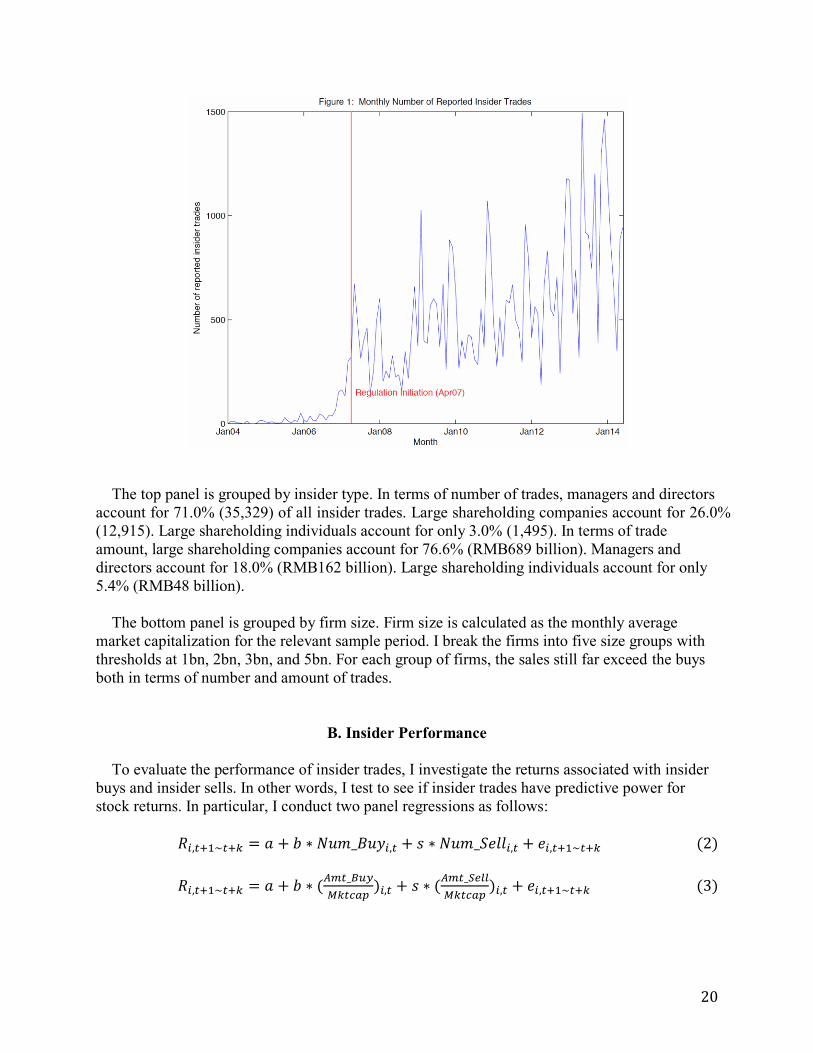
Figure 1 plots the time-series number of reported insider trades. Before the regulation on
insider reporting went into effect in April 2007, the reported insider trades were voluntary and
few in numbers. The sudden increase in reported trades took place in 2007. For the analysis that
follows, I use the data that start in April 2007.
Table 7 shows the summary statistics on Chinese insider trading activities from April 1, 2007
to June 30, 2014. In terms of number of trades, 74.3% of all insider trades are sales (36,977), far
more than insider buys (12,762). In terms of trade amount, 79.6% are attributed to insider sales
(RMB715 billion), and only 16.3% are purchases (RM184 billion).
20
The top panel is grouped by insider type. In terms of number of trades, managers and directors
account for 71.0% (35,329) of all insider trades. Large shareholding companies account for 26.0%
(12,915). Large shareholding individuals account for only 3.0% (1,495). In terms of trade
amount, large shareholding companies account for 76.6% (RMB689 billion). Managers and
directors account for 18.0% (RMB162 billion). Large shareholding individuals account for only
5.4% (RMB48 billion).
The bottom panel is grouped by firm size. Firm size is calculated as the monthly average
market capitalization for the relevant sample period. I break the firms into five size groups with
thresholds at 1bn, 2bn, 3bn, and 5bn. For each group of firms, the sales still far exceed the buys
both in terms of number and amount of trades.
B. Insider Performance
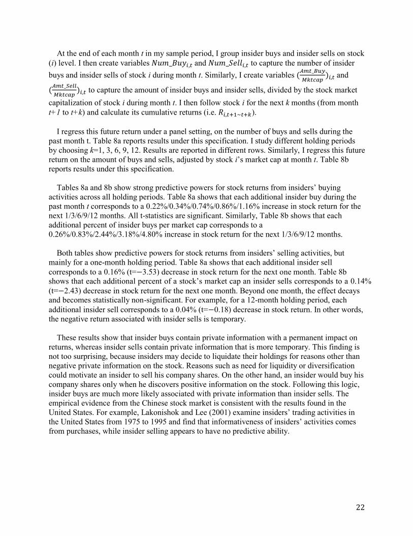
To evaluate the performance of insider trades, I investigate the returns associated with insider
buys and insider sells. In other words, I test to see if insider trades have predictive power for
stock returns. In particular, I conduct two panel regressions as follows:

21
Table 7
Insider Trading Summary Statistics The sample of insider trades covers the period from April 1, 2007 to June 30, 2014. It records a total of 49,739 trades of insiders from 2,275 publicly listed firms.
The top panel groups trades by insider type, i.e. manager/director, large shareholding company and large shareholding individual. The bottom panel groups trades
by the underlying firm size.
Manager /Director
Large Shareholder (Company)
Large Shareholder (Individual)
Total
Number of Trades
Purchases 10,173 2,252 337 12,762
Sales 25,156 10,663 1,158 36,977
Total 35,329 12,915 1,495 49,739
Amount of Trades (RMB million)
Purchases 21,682 156,064 6,022 183,768
Sales 140,540 532,619 42,144 715,303
Total 162,222 688,683 48,166 899,071
<1 billion 1~2 billion 2~3 billion 3~5 billion >5 billion Total
Number of Firms 319 638 430 386 502 2,275
Number of Trades
Purchases 878 2,991 2,186 2,093 4,614 12,762
Sales 4,375 11,124 7,774 5,410 8,294 36,977
Total 5,253 14,115 9,960 7,503 12,908 49,739
Amount of Trades (RMB million)
Purchases 2,418 14,122 12,110 21,182 133,937 183,768
Sales 25,032 122,410 110,455 129,541 327,865 715,303
Total 27,449 136,532 122,565 150,723 461,801 899,071
Grouped by Insider Type
Grouped by Firm Size
22
At the end of each month t in my sample period, I group insider buys and insider sells on stock
(i) level. I then create variables and to capture the number of insider
buys and insider sells of stock i during month t. Similarly, I create variables
and
to capture the amount of insider buys and insider sells, divided by the stock market
capitalization of stock i during month t. I then follow stock i for the next k months (from month
t+1 to t+k) and calculate its cumulative returns (i.e. ).
I regress this future return under a panel setting, on the number of buys and sells during the
past month t. Table 8a reports results under this specification. I study different holding periods
by choosing k=1, 3, 6, 9, 12. Results are reported in different rows. Similarly, I regress this future
return on the amount of buys and sells, adjusted by stock i’s market cap at month t. Table 8b
reports results under this specification.
Tables 8a and 8b show strong predictive powers for stock returns from insiders’ buying
activities across all holding periods. Table 8a shows that each additional insider buy during the
past month t corresponds to a 0.22%/0.34%/0.74%/0.86%/1.16% increase in stock return for the
next 1/3/6/9/12 months. All t-statistics are significant. Similarly, Table 8b shows that each
additional percent of insider buys per market cap corresponds to a
0.26%/0.83%/2.44%/3.18%/4.80% increase in stock return for the next 1/3/6/9/12 months.
Both tables show predictive powers for stock returns from insiders’ selling activities, but
mainly for a one-month holding period. Table 8a shows that each additional insider sell
corresponds to a 0.16% (t= 3.53) decrease in stock return for the next one month. Table 8b shows that each additional percent of a stock’s market cap an insider sells corresponds to a 0.14%
(t= 2.43) decrease in stock return for the next one month. Beyond one month, the effect decays and becomes statistically non-significant. For example, for a 12-month holding period, each
additional insider sell corresponds to a 0.04% (t= 0.18) decrease in stock return. In other words,
the negative return associated with insider sells is temporary.
These results show that insider buys contain private information with a permanent impact on
returns, whereas insider sells contain private information that is more temporary. This finding is
not too surprising, because insiders may decide to liquidate their holdings for reasons other than
negative private information on the stock. Reasons such as need for liquidity or diversification
could motivate an insider to sell his company shares. On the other hand, an insider would buy his
company shares only when he discovers positive information on the stock. Following this logic,
insider buys are much more likely associated with private information than insider sells. The
empirical evidence from the Chinese stock market is consistent with the results found in the
United States. For example, Lakonishok and Lee (2001) examine insiders’ trading activities in
the United States from 1975 to 1995 and find that informativeness of insiders’ activities comes
from purchases, while insider selling appears to have no predictive ability.

23
Table 8
Panel Regression Results on Insider Trade Performance and correspond to the number of insider buys and insider sells of stock i during month t.
Similarly,
and
correspond to the amount of insider buys and insider sells, divided by the
stock market capitalization of stock i during month t. are cumulative returns of stock i over the 1 to k
months starting at month t. Table 8a reports results from panel Regression (2), and Table 8b reports results from
panel Regression (3). The data cover insider trades from April 2007 to June 2013, for a total of 16,262 stock-month
data points.
Table 8a: Panel Regression Results using Num_Buy & Num_Sell
Holding Period
Constant Num_Buy Num_SellSample
SizeR-sq
0.91 0.22 -0.16
(5.91) (3.27) (-3.53)
3.91 0.34 -0.08
(13.00) (2.97) (-0.98)
7.04 0.74 -0.26
(13.87) (3.56) (-1.99)
10.60 0.86 -0.26
(15.51) (3.24) (-1.52)
12.62 1.16 -0.04
(14.62) (3.55) (-0.18)
Table 8b: Panel Regression Results using (Amt_Buy/Mktcap) & (Amt_Sell/Mktcap)
Holding Period
ConstantAmt_Buy/Mktcap
(%)Amt_Sell/Mktcap
(%)Sample
SizeR-sq
0.89 0.26 -0.14
(6.45) (1.30) (-2.43)
4.04 0.83 -0.16
(14.76) (2.70) (-1.64)
6.98 2.44 -0.25
(14.96) (4.47) (-1.65)
10.53 3.18 -0.27
(16.46) (5.10) (-1.41)
12.77 4.80 -0.14
(15.67) (5.89) (-0.61)
Standard errors are Newey-West adjusted.
16,262 0.4%
16,262 0.1%
16,262 0.3%
16,262 0.3%
16,262 0.1%
16,262 0.1%
16,262 0.1%
16,262 0.2%
16,262 0.1%
16,262 0.2%
12m
12m
6m
9m
1m
3m
1m
3m
6m
9m
C. Insider-Mimicking Strategy
Motivated by the panel regression results in Table 8a, I create a trading strategy that mimics
the insider trades. At the end of each month (starting from end of April 2007), I long one unit of
24
capital equally among all insider buys that took place during the past month. I hold these stocks
in my portfolio for the next 12 months and then sell them. I update my portfolio at the end of
each month following this strategy. Each month, I calculate the portfolio return as the current
month-end portfolio value divided by the last month-end portfolio value. Due to the 12-month
holding period on the positions, the portfolio takes 12 months to fully form. As a result, I
conduct analysis based on the portfolio returns from April 2008 to June 2014.
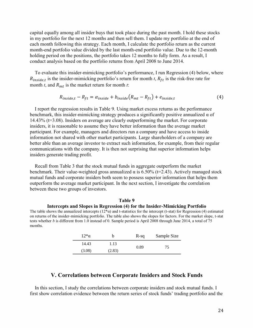
To evaluate this insider-mimicking portfolio’s performance, I run Regression (4) below, where
is the insider-mimicking portfolio’s return for month t, is the risk-free rate for
month t, and is the market return for month t:
I report the regression results in Table 9. Using market excess returns as the performance
benchmark, this insider-mimicking strategy produces a significantly positive annualized α of
14.43% (t=3.08). Insiders on average are clearly outperforming the market. For corporate
insiders, it is reasonable to assume they have better information than the average market
participant. For example, managers and directors run a company and have access to inside
information not shared with other market participants. Large shareholders of a company are
better able than an average investor to extract such information, for example, from their regular
communications with the company. It is then not surprising that superior information helps
insiders generate trading profit.
Recall from Table 3 that the stock mutual funds in aggregate outperform the market
benchmark. Their value-weighted gross annualized α is 6.50% (t=2.43). Actively managed stock
mutual funds and corporate insiders both seem to possess superior information that helps them
outperform the average market participant. In the next section, I investigate the correlation
between these two groups of investors.
Table 9
Intercepts and Slopes in Regression (4) for the Insider-Mimicking Portfolio The table shows the annualized intercepts (12*α) and t-statistics for the intercept (t-stat) for Regression (4) estimated
on returns of the insider-mimicking portfolio. The table also shows the slopes for factors. For the market slope, t-stat
tests whether b is different from 1.0 instead of 0. Sample period is April 2008 through June 2014, a total of 75
months.
12*α b R-sq Sample Size
14.43 1.13
(3.08) (2.83)750.89
V. Correlations between Corporate Insiders and Stock Funds
In this section, I study the correlations between corporate insiders and stock mutual funds. I
first show correlation evidence between the return series of stock funds’ trading portfolio and the

25
insider-mimicking portfolio. I then show that stock funds that trade more in correlation with
insiders deliver better performance. Finally, I offer more correlation evidence between mutual
funds’ large holdings and the insider-mimicking portfolio. Funds with a higher concentration in
such holdings outperform those with a lower concentration.
A. Return Correlation
As I discussed in section IV, both groups of investors, that is, corporate insiders and stock
funds, outperform the market benchmark significantly. To track the insiders’ performance, I use
the insider-mimicking portfolio constructed in section IV. This portfolio consists only of insider
buys because they contain more private information. To make proper comparisons, I construct a
trading portfolio for stock funds based on their buying activities. I then evaluate the performance
of both portfolios and show that they are significantly correlated.
A1. Aggregate-level Evidence
At the end of each semiannual period, I aggregate all stock funds’ holdings to form a big
portfolio. Equivalently, I can think of it as a big fund that holds the aggregate portfolio of all
stock funds. I track this big fund’s trading activities at the semiannual frequency. In particular, I
compare this fund’s holdings portfolios of adjacent periods and back out the positions it has
bought and sold during the last six months. More specifically, I measure its holding of a stock by
the holding’s value divided by the stock’s market capitalization. If this measure increases (or
decreases) from last period to this period, then I consider it a buy (or a sell).
I focus on the buys to construct the stock funds’ aggregate trading portfolio. After I form the
trading portfolio at the end of each semiannual period, I follow it for the next six months and
calculate the value-weighted buy-and-hold monthly portfolio returns. I then paste together the
six-month return series to form a longer monthly return series .
For the insider-mimicking portfolio, I first run the FF3F+MOM performance evaluation
regression, and then define an outperformance variable :
is the monthly outperformance series for the insider trading strategy. and
are the intercept and residuals of insider strategy. Because has mean zero,
should have mean , which is the monthly alpha of the insider-mimicking
portfolio. The outperformance monthly series helps capture the time-series variation of the
insider-mimicking portfolio’s performance, after adjusting for the market, size, value-growth and
momentum benchmarks.
Next, I evaluate the performance of the mutual funds’ aggregate trading portfolio, under the
FF3F+MOM model. I then add an additional factor to this regression:
26
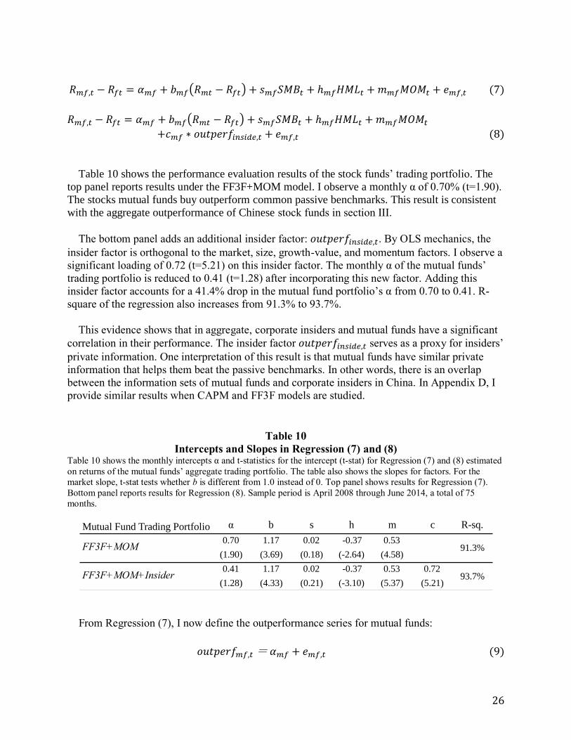
Table 10 shows the performance evaluation results of the stock funds’ trading portfolio. The
top panel reports results under the FF3F+MOM model. I observe a monthly α of 0.70% (t=1.90).
The stocks mutual funds buy outperform common passive benchmarks. This result is consistent
with the aggregate outperformance of Chinese stock funds in section III.
The bottom panel adds an additional insider factor: . By OLS mechanics, the
insider factor is orthogonal to the market, size, growth-value, and momentum factors. I observe a
significant loading of 0.72 (t=5.21) on this insider factor. The monthly α of the mutual funds’
trading portfolio is reduced to 0.41 (t=1.28) after incorporating this new factor. Adding this
insider factor accounts for a 41.4% drop in the mutual fund portfolio’s α from 0.70 to 0.41. R-
square of the regression also increases from 91.3% to 93.7%.
This evidence shows that in aggregate, corporate insiders and mutual funds have a significant
correlation in their performance. The insider factor serves as a proxy for insiders’
private information. One interpretation of this result is that mutual funds have similar private
information that helps them beat the passive benchmarks. In other words, there is an overlap
between the information sets of mutual funds and corporate insiders in China. In Appendix D, I
provide similar results when CAPM and FF3F models are studied.
Table 10
Intercepts and Slopes in Regression (7) and (8) Table 10 shows the monthly intercepts α and t-statistics for the intercept (t-stat) for Regression (7) and (8) estimated
on returns of the mutual funds’ aggregate trading portfolio. The table also shows the slopes for factors. For the
market slope, t-stat tests whether b is different from 1.0 instead of 0. Top panel shows results for Regression (7).
Bottom panel reports results for Regression (8). Sample period is April 2008 through June 2014, a total of 75
months.
Mutual Fund Trading Portfolio α b s h m c R-sq.
0.70 1.17 0.02 -0.37 0.53
(1.90) (3.69) (0.18) (-2.64) (4.58)
0.41 1.17 0.02 -0.37 0.53 0.72
(1.28) (4.33) (0.21) (-3.10) (5.37) (5.21)FF3F+MOM+Insider 93.7%
FF3F+MOM 91.3%
From Regression (7), I now define the outperformance series for mutual funds:
=

27
and are simply the intercept and residual series from Regression (7). Similar to
, captures the time-series variation of the mutual funds’ trading
portfolio’s performance, after adjusting for the market, size, value-growth and momentum
benchmarks.
The correlation between and is 0.53 with a t-statistic of 5.36. This
significantly positive correlation suggests mutual funds and insiders tend to win and lose to the
passive benchmarks at the same time. Figure 2 plots the 3-month moving average of both
outperformance series. They have a correlation of 0.32 with a t-statistic of 3.24 (standard errors
are Newey-West adjusted). Given this aggregate correlation evidence, I conjecture that stock
funds and insiders share some private information that helps them beat the market. In Appendix
E, I provide results using a placebo portfolio instead of the mutual funds’ trading portfolio. I show the placebo portfolio has no statistically significant correlation with the insider factor.
A2. Fund-level Evidence
I now turn to study the fund-level correlations with the insider factor . First, for
each fund i in my sample, I construct its trading portfolio from its semiannual holdings data. I
then follow this portfolio for the next six months and calculate the value-weighted buy-and-hold
monthly portfolio returns. Next, I paste together the fund’s six-month return series to form a
longer monthly return series . Basically, I apply the same methodology as in subsection A1,
but to each fund i in my sample instead of the aggregate fund portfolio.
To study the correlations between individual funds’ trading portfolios and the insider-
mimicking portfolio, I run the following regression for each mutual fund i in my sample:

28
Table 11 exhibits the percentile distribution for coefficient , its t-statistic and the fraction of
variance due to the insider factor . Specifically, this fraction is defined as
.
The average fund loads significantly (c=0.91, t=2.00) on the insider factor. Median/mean
variance decomposition is 2.38%/3.82%, with a fairly wide range from 0.00% to 31.89%.
Consistent with the aggregate-level correlation evidence, I observe that cross-sectionally, about
half of the funds correlate significantly with the insider portfolio.
Table 11
Summary Statistics for Correlation Coefficient in Regression (10) For a given fund i, I perform Regression (10) to obtain its coefficient on the term. Defined in
equation (6), is a monthly time series of the insider-mimicking strategy’s outperformance against
the benchmarks including market, size, growth-value, and momentum. Table 11 shows the distribution summary
statistics of coefficient , its t-statistics, and the fraction of variance explained by the insider factor .
I require the funds to report at least two years of holdings data to be considered in this exercise. The sample includes
a total of 271 funds.
Distribution c t(c) fraction_insider
min -1.20 -1.56 0.00
10% 0.11 0.23 0.19
25% 0.44 1.05 0.90
50% 0.77 1.90 2.38
mean 0.91 2.00 3.82
75% 1.31 2.87 5.45
90% 1.94 3.91 8.96
max 3.58 6.19 31.89
B. Trading Correlation
In this section, I investigate mutual fund trading in connection with insider trading. I show that
mutual funds that exhibit more correlated trading patterns with insiders deliver better
performance.
Stock mutual funds report their entire stock holdings every six months. As a result, I observe
what a fund i has traded during a six-month period t. If a fund’s holding in a stock
increases/decreases during the period, it is considered a buy/sell. If a fund’s holding in a stock
does not change during the six-month period, it is considered no action. Obviously, if a stock
does not show up in the holdings report either at the start or the end of the period, it would not be
considered in the calculation for fund i’s trading in period t.

29
For the same six-month period t, I generate the list of stocks that have at least one insider buy.
As discussed in section IV, insider buys are much more likely than insider sells to contain private
information. In the spirit of focusing on more relevant inside information reflected by their trades,
I focus on the insider buys and ignore the insider sells.
Next, for a given mutual fund i and six-month period t, I count their overlapped stocks with
insiders, that is, stocks that are traded (include all types: buy, sell, and no action) by the mutual
fund i and bought at least once by insiders, during period t. I impose a threshold of 15 for a fund
to be considered in the sample. I then create a variable equal to the fraction of overlapped stocks
the mutual fund has bought in this six-month period. I call this variable , which is
designed to reflect the correlation in trading patterns between a fund i and insiders, during period
t. For example, if a fund i during period t has 25 overlapped stocks with insiders, and the fund
has increased its holding in 20 of these 25 stocks, then .
Because my insider data set starts in April 2007, and mutual funds report end-of-June and end-
of-December stock holdings, my sample for this exercise starts with the six-month period
July2007-Dec2007, and ends with July2013-Dec2013. For each six-month period, I create a fund
sample following the procedure described above. I then sort funds into quartile portfolios by
. Quartile 1 funds have the lowest and Quartile 4 funds have the
highest . I then follow the quartiles for the next six months and calculate the equal-
weighted average returns of each quartile portfolio. I then paste the monthly quartile portfolio
return series to form a long return series from January 2008 to June 2014, for a total of 78
months. I also construct a long-short portfolio by subtracting returns of Quartile 1 from Quartile
4.
I then evaluate each portfolio’s performance by the CAMP, FF3F, and FF3F+MOM models.
Table 12 summarizes the regression results. An increasing trend is present in the quartile
performance. That is, the more correlated a fund’s trading is with the insiders’ trading, the better
performance it is going to deliver. Under the CAMP, FF3F, and FF3F+MOM models, the long-
short fund portfolio produces a significantly positive monthly α of 0.20% (t=2.62), 0.19%
(t=2.31), and 0.18% (t=2.26) respectively.
Table 12
Performance of Quartile Fund Cohorts Sorted by Trading Correlation with Insiders For a given semiannual period t and a given fund i, I calculate the fund’s trading correlation with insiders as
. To calculate , I compare the overlapped stocks between fund i and the insiders during
period t, defined as those stocks that are bought by at least one insider and show up in the fund’s portfolio. I define
as the fraction of these overlapped trades that fund i bought during period t.
For each semiannual period, I sort funds into quartile cohorts by their . I follow these quartile cohorts
for the next six months and calculate each quartile’s monthly return series. Then I paste the six-month return series
together to create a longer return series for each quartile cohort. Quartile 1 funds have the lowest . Quartile 4 funds have the highest . I run the CAPM and FF3F versions of Regression (1) to obtain a
monthly α for each quartile cohort, as well as a long-short portfolio constructed from subtracting Quartile 1 returns
from Quartile 4 returns. Table 12 reports regression statistics on α for the CAPM, FF3F and FF3F+MOM
specifications. The sample covers a period from July 2003 to June 2014.

30
trade_corr α t(α) α t(α) α t(α)
Quartile 1 (bottom) 0.23 (1.07) 0.46 (2.59) 0.43 (2.65)
Quartile 2 0.33 (1.45) 0.52 (2.72) 0.50 (2.68)
Quartile 3 0.29 (1.28) 0.54 (2.79) 0.51 (2.88)
Quartile 4 (top) 0.43 (1.91) 0.65 (3.42) 0.62 (3.58)
4-1 0.20 (2.62) 0.19 (2.31) 0.18 (2.26)
CAPM FF3F FF3F+MOM
This cross-sectional evidence corroborates the aggregate correlation evidence discovered in
subsection A. The aggregate return correlation evidence shows that mutual funds in aggregate
have some information overlap with corporate insiders. As a result, they tend to win or lose
against the passive benchmarks at the same time. In this subsection, I show that amongst the
mutual funds that exhibit a sufficient number of overlapped trades with insider trades, the more
correlated the mutual fund trading is with the insiders, the better performance it delivers.
Last but not least, the fact that a fund trades in concordance with insiders does not necessarily
mean they are illegally trading on inside information. In fact, their trading decisions could be
derived from research on public information. I am merely claiming that more correlated trading
points to a higher likelihood of a common private information set between mutual funds and
corporate insiders. Due to the limitation of my data, I cannot make a further claim on how fund
managers obtain this private information. If we consider the similarity in trading patterns a proxy
for access to inside information, then funds with better access to inside information clearly
outperform those with worse access to inside information.
C. Qualified Holding Correlation
Conceivably, a fund is more likely to gain access to insiders’ private information if it is a large
shareholder of the company. To capture this notion, I create a variable mfmkt% defined as the
value of a mutual fund’s holding of a stock divided by the stock’s market capitalization.
Furthermore, I define a fund’s qualified holdings as those stocks with mfmkt% exceeding a given
threshold. In other words, a fund’s qualified stock holdings represent a large shareholding
percentage of the corresponding companies.
C1. Aggregate-level Evidence I construct a portfolio of stock funds’ aggregate qualified holdings. Specifically, from each
fund’s semiannual holdings, I keep the stocks with mfmkt% exceeding a given threshold
(0.50%,1.00%, 1.50%, and 2.00%). I then aggregate such stocks across all funds to form a single
portfolio that I buy and hold for the next six months. I update this portfolio of aggregate qualified
holdings every six months. I then paste the six-month return series together to form a long
monthly return series. The resulting monthly return series captures the performance of stock
funds’ aggregate qualified holdings.
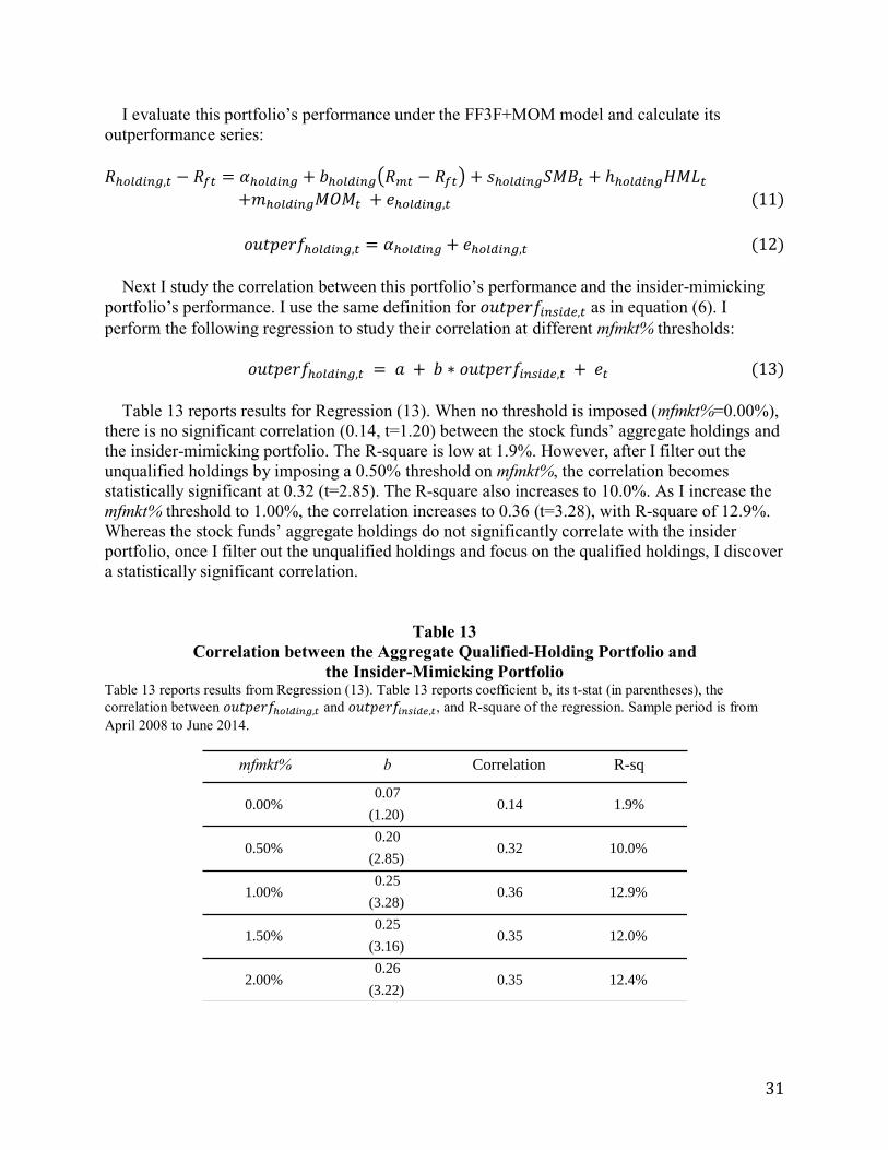
31
I evaluate this portfolio’s performance under the FF3F+MOM model and calculate its
outperformance series:
Next I study the correlation between this portfolio’s performance and the insider-mimicking
portfolio’s performance. I use the same definition for as in equation (6). I
perform the following regression to study their correlation at different mfmkt% thresholds:
Table 13 reports results for Regression (13). When no threshold is imposed (mfmkt%=0.00%),
there is no significant correlation (0.14, t=1.20) between the stock funds’ aggregate holdings and
the insider-mimicking portfolio. The R-square is low at 1.9%. However, after I filter out the
unqualified holdings by imposing a 0.50% threshold on mfmkt%, the correlation becomes
statistically significant at 0.32 (t=2.85). The R-square also increases to 10.0%. As I increase the
mfmkt% threshold to 1.00%, the correlation increases to 0.36 (t=3.28), with R-square of 12.9%.
Whereas the stock funds’ aggregate holdings do not significantly correlate with the insider
portfolio, once I filter out the unqualified holdings and focus on the qualified holdings, I discover
a statistically significant correlation.
Table 13
Correlation between the Aggregate Qualified-Holding Portfolio and
the Insider-Mimicking Portfolio Table 13 reports results from Regression (13). Table 13 reports coefficient b, its t-stat (in parentheses), the
correlation between and , and R-square of the regression. Sample period is from
April 2008 to June 2014.
mfmkt% b Correlation R-sq
0.07
(1.20)
0.20
(2.85)
0.25
(3.28)
0.25
(3.16)
0.26
(3.22)2.00% 0.35 12.4%
0.50% 0.32 10.0%
12.0%1.50% 0.35
1.00% 0.36 12.9%
0.00% 0.14 1.9%

32
These results are consistent with the intuition that large shareholders may have better access to
insiders’ private information. For example, large shareholders are more likely to have regular
communications with company insiders. Through meetings, phone calls and other forms of
communication, large shareholders of a company can more easily obtain private information
from company insiders.
C2. Fund-level Evidence
Based on last subsection’s results, I make an assumption that large shareholders of a company
are more likely to have access to inside information than smaller shareholders. In my notation, a
stock fund is a large shareholder of a company if it has a high mfmkt% in that stock. My
assumption implies that within a fund’s portfolio, those holdings with a high mfmkt% are more
likely to have access to insiders’ private information. From section IV, I have already observed
that insiders’ superior information leads to superior performance. Therefore, I test the following
hypothesis:
Funds with a higher average holding concentration in qualified holdings outperform funds
with a lower average holding concentration.
I construct a holding-concentration variable that serves as a proxy for the amount of inside
information a fund has access to. For a given reporting period and fund, the holding
concentration is defined as the weight of a fund’s portfolio that is invested in qualified holdings,
adjusted by the stocks’ weights in the market benchmark portfolio.
A simple example will illustrate the calculation for the holding-concentration variable. The
mfmkt% threshold is set at 1.0%. A fund holds N qualified stocks with mfmkt%>1.0% in a given
period. The fund’s holdings in these N stocks account for of its stock
portfolio. The market capitalization of these N stocks account for of the
market portfolio. Then the holding concentration of the fund for the given period is defined as
. If N is zero (i.e. there is no qualified stock), I assign value zero to the fund’s
holding concentration for the period.
I calculate each fund’s holding concentration for every period. I then define each fund’s
average holding concentration as the equal-weighted average value of its holding concentrations
across all periods.
This holding-concentration measure captures a given fund’s asset concentration in the
qualified stocks, adjusted by those qualified stocks’ market portfolio weights. It measures the
fund’s deviation from the market benchmark portfolio on those qualified stocks. A fund would
have a high holding concentration if it holds a large portion of its portfolio in qualified stocks,
and it overweighs those stocks relative to the market portfolio.
I then perform a cross-sectional test to see if funds with a higher average holding
concentration outperform funds with a lower average holding concentration. I first run a
FF3F+MOM regression for each fund i and record their values:

33
I then regress these on their holding concentration ( ) variable:
I calculate the holding concentration at two reporting frequencies: quarterly and semiannual.
As discussed before, funds report top-10 holdings at the quarterly frequency and entire holdings
at the semiannual frequency. On average, the top-10 holdings of a fund account for 49.8% of the
fund’s overall stock portfolio. I present quarterly and semiannual results in Tables 14a and 14b
respectively. For quarterly results, I show results for different mfmkt% thresholds from 0.00% to
2.00%. For semiannual results, I show results for different mfmkt% thresholds from 0.50% to 2.00%.
Table 14a first shows the results when I impose no threshold on mfmkt%. For quarterly data,
mfmkt%=0.00% threshold corresponds to a fund’s top-10 holdings, which do not necessarily
represent a large shareholding percentage of the stock. The loading on the top-10 concentration
( =0.51, t=1.49) implies the relationship between the funds’ performance and their top-10
holding concentrations is statistically non-significant.
More interestingly, when I impose a 0.50% threshold on mfmkt%, results become much more
significant: =1.71 (t=6.62). R-square increases substantially from 0.6% (under 0.00% threshold) to 10.2% (under 0.50% threshold). As I increase the mfmkt% threshold, I observe similar results
that funds’ holding concentrations correlate significantly with funds’ performance.
Table 14b shows similar results using holding concentration constructed from semiannual
holdings data. I also observe a significant correlation between funds’ performance and their
holding concentrations. For example, given a 0.50% threshold on mfmkt%, I observe =0.95 (t=6.36), with a R-square of 9.5%.
Under the assumption that higher mfmkt% implies better access to inside information, my
holding-concentration measure reflects a fund’s overall access to inside information. A fund with
a higher concentration would have better access to inside information. Given the valuable private
information possessed by insiders, better access to such information should produce better fund
performance. The correlation results between funds’ performance and their holding
concentrations are consistent with this intuition.
Table 14
Fund Performance and Holding Concentration As in Regression (14), I compute the FF3F α for each fund in my sample. Next, I impose the mfmkt% threshold and
select qualified holdings for each fund and reporting period. I compute each fund’s qualified holding concentration
for every reporting period. I define a fund’s holding concentration as the equal-weighted average value from all
reporting periods. I assign value zero to any fund-period combination that reported no stock that meets the mfmkt%
threshold. I report the quarterly results in the top panel and the semiannual results in the bottom panel.

34
Table 14a: Fund FF3F+MOM α vs. Holding Concentration (Quarterly)
mfmkt% ConstantHolding
ConcentrationR-sq. Sample Size
0.14 0.51
(0.85) (1.49)
0.09 1.71
(1.57) (6.62)
0.14 2.23
(2.88) (6.40)
0.18 2.74
(3.85) (6.16)
0.22 3.12
(4.77) (5.68)
Table 14b: Fund FF3F+MOM α vs. Holding Concentration (Semiannual)
mfmkt% ConstantHolding
ConcentrationR-sq. Sample Size
0.11 0.95
(2.01) (6.36)
0.18 1.23
(3.57) (6.05)
0.22 1.48
(4.63) (5.59)
0.25 1.70
(5.55) (5.05)
0.00% 0.6% 386
0.50% 10.2% 386
1.00% 9.6% 386
1.50% 9.0% 386
2.00% 7.8% 386
0.50% 9.5% 385
2.00% 6.3% 385
1.00% 8.7% 385
1.50% 7.5% 385
VI. Performance Erosion of Stock Mutual Funds
In this section, I present evidence of performance erosion for Chinese stock mutual funds, in
connection with the growth of the institutional money management industry. Performance
erosion of stock funds suggests the Chinese stock market is becoming more efficient and harder
to beat. I also show that the aggregate stock fund portfolio becomes closer to the market portfolio
over time.
1. Performance Erosion of Stock Mutual Funds
I add a time trend to Regression (1) to capture the performance erosion of stock mutual funds.
I use the aggregate value-weighted fund gross returns in Regression (16):

35
Table 15 shows results for the CAPM, FF3F, and FF3F+MOM versions of Regression (16).
Under all three specifications, I observe a negative time trend in benchmark-adjusted returns. For
example, under CAPM, the monthly performance decay is 0.01% (t= 1.75), which translates
into an annual performance decay of 0.12%. For my sample period from 2003 to 2014, the
performance decay amounts to 1.32%. Under FF3F and FF3F+MOM models, monthly
performance erosion is 0.009% (t= 2.12) and 0.008% (t= 2.23) respectively. Although the
mutual funds outperform passive benchmarks during my sample period from 2003 to 2014, their
performance seems to have been decaying over time.
Table 15
Performance Erosion of Stock Mutual Funds Table 15 shows the monthly intercepts α and t-statistics for the intercept (t-stat) for the CAPM, FF3F, and
FF3F+MOM versions of Regression (16) estimated on value-weight (VW) gross returns on the portfolios of actively
managed stock mutual funds. The table also shows the slopes for benchmark factors and time trend. For the market
slope, t-stat tests whether b is different from 1.0 instead of 0. The period is July 2003 through June 2014. The data
cover 418 funds.
α RmRf SMB HML MOM Time (Month) R-sq.
1.22 0.71 -0.010
(2.73) (-11.56) (-1.75)
1.50 0.77 -0.27 -0.46 -0.009
(4.77) (-13.08) (-7.83) (-8.84) (-2.12)
1.35 0.78 -0.21 -0.35 0.23 -0.008
(4.73) (-13.70) (-6.37) (-6.85) (5.53) (-2.23)
CAPM
FF3F
FF3F+MOM
86.7%
93.7%
94.9%
The results on performance erosion are consistent with the intuition that the Chinese stock
market is becoming more efficient. The improvement in the Chinese stock market’s efficiency
may be attributed to the increasing competition from institutional money managers. Next, I show
summary statistics on the Chinese institutional money-management industry.
2. Growth of the Institutional Money Management Industry
I compile the semiannual stock holdings data of the Chinese institutional investors. Table 16
reports summary statistics on Chinese institutional stock holdings, in relation to the aggregate
stock market capitalization and stock mutual fund AUM. At the end of 2003, Chinese
institutional investors represented only 12.5% of the aggregate stock market capitalization.
Within the institutional holdings, stock mutual funds represented a substantial 40.8%. In addition,
Chinese retail investors were the dominant fraction in the stock market then, holding over 87%
of the stock market. This period was a great time for professional money managers because the
competition from other institutional investors was low and many retail investors were in the

36
market. Professional money managers have more knowledge and resources than retail investors,
so they are positioned to outperform them. In other words, they were beating the market easily at
the expense of many retail investors.
Table 16
Summary Statistics on Institutional Stock Holdings Table 16 reports summary statistics on Chinese institutional stock holdings, in relation to the aggregate stock market
capitalization and stock mutual fund AUM. The institutional holdings data was initiated in the fourth quarter of 2003.
Column 1 records the semiannual reporting period. Column 2 shows the aggregate Chinese stock market
capitalization. Column 3 shows the value of aggregate Chinese institutional stock holdings. Column 4 shows the
institutional fraction of the stock market capitalization. Column 5 shows the aggregate AUM of Chinese stock
mutual funds. Column 6 shows the stock funds’ fraction of the stock market capitalization. Column 7 shows the
ratio between the aggregate stock funds’ AUM and the value of aggregate institutional stock holdings.
Reporting Period
Aggr. Stock MktCap (bn)
Institutional Stock
Holding (bn)
Institutional Holding %
Stock Fund AUM (bn)
Stock Fund AUM %
Stock Fund / Institutional
Holding
4Q/2003 ¥1,244 155 12.5% ¥63 5.1% 40.8%
2Q/2004 ¥1,204 177 14.7% ¥63 5.2% 35.6%
4Q/2004 ¥1,116 204 18.3% ¥66 5.9% 32.1%
2Q/2005 ¥953 199 20.8% ¥67 7.1% 33.8%
4Q/2005 ¥1,020 231 22.7% ¥88 8.7% 38.2%
2Q/2006 ¥1,619 355 21.9% ¥150 9.3% 42.4%
4Q/2006 ¥2,412 758 31.4% ¥377 15.6% 49.7%
2Q/2007 ¥5,413 1,882 34.8% ¥813 15.0% 43.2%
4Q/2007 ¥9,140 3,798 41.6% ¥1,515 16.6% 39.9%
2Q/2008 ¥5,919 2,453 41.4% ¥873 14.7% 35.6%
4Q/2008 ¥4,538 2,059 45.4% ¥636 14.0% 30.9%
2Q/2009 ¥9,084 4,597 50.6% ¥953 10.5% 20.7%
4Q/2009 ¥15,074 9,349 62.0% ¥1,049 7.0% 11.2%
2Q/2010 ¥12,668 7,828 61.8% ¥846 6.7% 10.8%
4Q/2010 ¥19,232 12,444 64.7% ¥989 5.1% 7.9%
2Q/2011 ¥20,051 13,078 65.2% ¥902 4.5% 6.9%
4Q/2011 ¥16,517 11,092 67.2% ¥747 4.5% 6.7%
2Q/2012 ¥17,337 11,408 65.8% ¥749 4.3% 6.6%
4Q/2012 ¥18,220 12,094 66.4% ¥739 4.1% 6.1%
2Q/2013 ¥16,979 10,919 64.3% ¥724 4.3% 6.6%
4Q/2013 ¥20,039 12,752 63.6% ¥758 3.8% 5.9%
Over time, we see two trends taking place simultaneously. First, the institutional investors are
managing more and more assets. Stocks held by Chinese institutional investors have grown from
RMB155 billion to RMB12,752 billion in 10 years. The fraction of the stock market held by
institutional investors increased from 12.5% to 63.6%. Second, within institutional investors,
stock mutual funds’ presence is waning, decreasing from 40.8% to 5.9%. This decrease means a

37
lot of other types of professional money managers are entering the institutional money-
management industry, for example, banks, insurance companies, brokerage firms, and trusts.
They are gaining clout within institutional money management. Both trends are likely hurting the
performance of stock mutual funds. Fewer retail investors and more professional investors in the
market lead to fiercer competition. Market participants become more efficient in processing
public information. They may also compete for private information. Facing more competition
from fellow professional money managers, stock mutual funds are seeing their performance
erode over time.
Pastor, Stambaugh, and Taylor (2014) find similar evidence of rising competition in the U.S.
stock market. They find that the rising competition is offset by the rising skill of active mutual
funds, so that the net effect on the performance of U.S. active funds is approximately neutral. In
contrast, I find that competition in China has risen so fast that the performance of Chinese funds
has declined over time.
Last but not least, the Chinese regulatory authority’s harsher punishment for insider trading
may also contribute to the improvement in the Chinese stock market’s efficiency. The private
information channel that used to help some fund managers beat the market is being gradually
shut down. As a result, those fund managers are seeing their performance decline over time.
VII. Conclusion
In this paper, I investigate private information in the Chinese stock market by studying two
groups of Chinese investors: stock mutual funds and corporate insiders. First, I find in aggregate,
these stock funds outperform passive benchmarks including market, size, value-growth, and
momentum factors. Bootstrap simulations based on a zero-α return sample suggest that most
Chinese stock fund managers have sufficient skill to cover all costs and generate α. Using funds’
semiannual stock holdings data, I find managers possess skill in stock selection that help explain
a substantial amount of the funds’ α.
Next, I discover direct evidence of information asymmetry in the Chinese stock market.
Chinese corporate insiders generate abnormal profits by trading their own company stocks. The
positive return associated with insider buys is strong and lasts for at least 12 months. The
negative return associated with insider sells is strong in the short term (one month) but quickly
decays. Based on these results, I construct an insider trading strategy and show this simple
insider-mimicking portfolio produces a significantly positive annual alpha of 14.43% (t=3.08)
against the market benchmark.
I then show a strong correlation between the performance of stock mutual funds and corporate
insiders. First, I show a strong correlation between the performance of stock funds’ trading
portfolio and the insider-mimicking portfolio. Second, I find that funds trading more in
correlation with insiders deliver better performance. Finally, I find that stock funds’ large share
positions exhibit a significant return correlation with insiders’ portfolio. Furthermore, funds with
a higher concentration in these positions outperform those funds with a lower concentration.

38
Finally, I present evidence of performance erosion for Chinese stock mutual funds, showing
that the Chinese stock market is becoming more efficient and harder to beat. This result is
consistent with more competition among professional money managers, better financial
regulation, and harsher crackdowns on insider trading. I see this improvement in market
efficiency as an encouraging sign for the future development of Chinese financial markets.
REFERENCES
Admati Anat R., and Paul Pfleiderer, 1986, A Monopolistic Market for Information, Journal of Economic
Theory 39, 400-438.
Baks, Klaas P., 2002, On the performance of mutual fund managers, Working paper, Emory University.
Barber Brad M., and Terrance Odean, 2000, Trading is hazardous to your wealth: the common stock
investment performance of individual investors, Journal of Finance 55, 773–806.
Barber Brad M., Yi-Tsung Lee, Yu-Jane Liu, and Terrance Odean, 2013, The cross-section of speculator
skill: evidence from day trading, Working paper, UC Davis.
Barras Laurent, Olivier Scaillet, and Russ Wermers, 2010, False Discoveries in Mutual Fund Performance:
Measuring Luck in Estimated Alphas, Journal of Finance Vol. LXV, No. 1, 179–216.
Berk, Jonathan B., and Richard C. Green, 2004, Mutual fund flows in rational markets, Journal of
Political Economy 112, 1269–1295. Berk, Jonathan B., and Jules H. van Binsbergen, 2014, Measuring Skill in the Mutual Fund Industry, Working
Paper. Bollen, Nicolas P. B., and Jeffrey A. Busse, 2001, On the Timing Ability of Mutual Fund Managers,
Journal of Finance Vol. LVI, No. 3, 1075–1094. Bollen, Nicolas P. B., and Jeffrey A. Busse, 2005, Short-term persistence in mutual fund performance,
Review of Financial Studies 18, 569–597. Brown, Stephen J., and William N. Goetzmann, 1995, Performance persistence, Journal of Finance
50, 679–698.
Brown, Stephen J., William N. Goetzmann, Roger G. Ibbotson, and Stephen A. Ross, 1992,
Survivorship bias in performance studies, Review of Financial Studies 5, 553–580.
Busse, Jeffrey A., and Paul J. Irvine, 2006, Bayesian alphas and mutual fund persistence, Journal of Finance 61,
2251-2288.
Carhart, Mark M., 1997, On persistence in mutual fund performance, Journal of Finance 52, 57–82.
Carhart, Mark M., Ron Kaniel, David K. Musto, and Adam V. Reed, 2002, Learning for the tape:
Evidence of gaming behavior in equity mutual funds, Journal of Finance 57, 661–693.
Chang, Xin, Shi Hua Lin, Lewis H.K. Tam, and George Wong, 2010, Cross-sectional determinants of post-
IPO stock performance: evidence from China, Accounting and Finance 50, 581–603.
Chen, Joseph, Harrison Hong, Ming Huang, and Jeffrey Kubik, 2004, Does fund size erode mutual fund
performance, American Economic Review 94, 1276–1302.
Chen, Hsiu-Lang, Narasimhan Jegadeesh, and Russ Wermers, 2000, The value of active mutual fund
management: An examination of the stockholdings and trades of fund managers, Journal of
Financial and Quantitative Analysis 35, 343–368.
Chin, Shengtyng, and Changyun Wang, 2004, Profitability of return and volume-based investment
strategies in China’s stock market, Pacific-Basin Finance Journal 12, 541–564.
Choi, James, Li Jin, and Hongjun Yan, 2014, Informed trading and expected returns, NBER Working Paper
No. 18680.
Cohen, Randolph B, Joshua D. Coval, and Lubos Pastor, 2005, Judging fund managers by the company
they keep, Journal of Finance 60, 1057–1096.
Cremers, Martijn, and Antti Petajisto, 2009, How active is your fund manager? A new measure
that predicts performance, Review of Financial Studies 22, 3329–3365.
Daniel, Kent D., Mark Grinblatt, Sheridan Titman, and Russ Wermers, 1997, Measuring mutual fund
performance with characteristic-based benchmarks, Journal of Finance 52, 1035–1058.

39
Dybvig, Philip H., and Stephen A. Ross, 1985, The analytics of performance measurement using a security
market line, Journal of Finance 40, 401–416.
Elton, Edwin J., Martin J. Gruber, and Christopher R. Blake, 1996, The persistence of risk-adjusted mutual
fund performance, Journal of Business 69, 133–157.
Elton, Edwin J., Martin J. Gruber, and Christopher R. Blake, 2001, A first look at the accuracy of the CRSP
mutual fund database and a comparison of the CRSP and Morningstar mutual fund databases, Journal
of Finance 56, 2415–2430.
Evans, Richard, 2003, Does alpha really matter? Evidence from mutual fund incubation, termination and
manager change, Working paper, Wharton.
Evans, Richard, 2010, Mutual fund incubation, Journal of Finance 65, 1581–1611.
Fama, Eugene F., 1965, The behavior of stock market prices, Journal of Business 38, 34–105.
Fama, Eugene F., 1970, “Efficient Capital Markets: A Review of Theory and Empirical Work,” Journal of
Finance, 25(2), 383–417.
Fama, Eugene F., and Kenneth R. French, 1993, Common risk factors in the returns on stocks and bonds,
Journal of Financial Economics 33, 3–56.
Fama, Eugene F., and Kenneth R. French, 2010, Luck versus Skill in Mutual Fund Returns, Journal of
Finance 5, 1915–1947.
Ferson, Wayne E., and Rudi W. Schadt, 1996, Measuring fund strategy and performance in changing
economic conditions, Journal of Finance 51, 425–462.
Ferson, Wayne E., and Kenneth Khang, 2002, Conditional performance measurement using portfolio
weights: Evidence for pension funds, Journal of Financial Economics 65, 249–282.
Finnerty Joseph E., 1976, Insiders and Market Efficiency, Journal of Finance Vol. XXXI, No. 4, 1141–
1148.
French, Kenneth R., 2008, The cost of active investing, Journal of Finance 63, 1537–1573.
Henriksson R., and R. Merton, 1981, On Market Timing and Investment Performance, Journal of Business
54 (4), 513–533.
Goetzmann, William N., and Roger G. Ibbotson, 1994, Do winners repeat? Patterns in mutual fund
performance, Journal of Portfolio Management 20, 9–18.
Grinblatt, Mark, and Sheridan Titman, 1989, Mutual fund performance: An analysis of quarterly
portfolio holdings, Journal of Business 62, 394–415.
Grinblatt, Mark, and Sheridan Titman, 1992, Performance persistence in mutual funds, Journal of Finance
47, 1977–1984.
Grinblatt, Mark, Sheridan Titman, and Russ Wermers, 1995, Momentum investment strategies, portfolio
performance, and herding: A study of mutual fund behavior, American Economic Review 85, 1088–
1105.
Grossman, Sanford, and Joseph E. Stiglitz, 1980, On the Impossibility of Informationally Efficient
Markets, American Economic Review Vol. 70, No. 3, 393–408.
Gruber, Martin J., 1996, Another puzzle: The growth of actively managed mutual funds, Journal of
Finance 51, 783–810.
Grundy, Bruce D., and J. Spencer Martin, 2001, Understanding the nature of the risks and the sources of
the rewards to momentum investing, Journal of Financial Studies 14, 29–78.
Haugen, Robert A., and Josef Lakonishok, 1988, The Incredible January Effect: The Stock Market’s
Unsolved Mystery (Dow Jones–Irwin, Homewood, IL).
Hellwig, Martin F., 1980, On the Aggregation of Information in Competitive Markets, Journal of Economic
Theory 22, 477–498.
Hendricks, Darryl, Jayendu Patel, and Richard Zeckhauser, 1993, Hot hands in mutual funds:
Short-run persistence of relative performance, 1974–1988, Journal of Finance 48, 93–130.
Hong, Harrison, Jeffrey D. Kubik, and Jeremy C. Stein, 2005, Thy neighbor’s portfolio: Word-
of-mouth effects in the holdings and trades of money managers, Journal of Finance 60, 2801–2824.
Ippolito, Richard A., 1992, Consumer reaction to measures of poor quality: Evidence from the mutual fund
industry, Journal of Law and Economics 35, 45–70.
Jaffe, Jeffrey F., 1974, Special information and insider trading, The Journal of Business, 47(3), 410-428.
Jensen, Michael C., 1968, The performance of mutual funds in the period 1945–1964, Journal of Finance
23, 2033–2058.
Jiang, George J., Tong Yao, and Tong Yu, 2007, Do mutual funds time the market? Evidence from
portfolio holdings, Journal of Financial Economics 86, 724-758.

40
Jones, Christopher S., and Jay Shanken, 2005, Mutual fund performance with learning across funds,
Journal of Financial Economics 78, 507–552.
Kacperczyk, Marcin, Clemens Sialm, and Lu Zheng, 2005, On the Industry Concentration of Actively Managed
Equity Mutual Funds, Journal of Finance Vol. LX, No. 4, 1983–2011.
Kacperczyk, Marcin, and Amit Seru, 2007, Fund Manager Use of Public Information: New Evidence on
Managerial Skills, Journal of Finance Vol. LXII, No. 2, 485–528.
Korajczyk, Robert A., and Ronnie Sadka, 2004, Are momentum profits robust to trading costs? Journal of
Finance 59, 1039–1082.
Kosowski, Robert, Allan Timmermann, Russ Wermers, and Hal White, 2006, Can mutual fund “stars”
really pick stocks? New evidence from a bootstrap analysis, Journal of Finance 61, 2551–2595.
Lakonishok, Josef, and Inmoo Lee, 2001, Are Insider Trades Informative, Review of Financial Studies
14(1), 79–111.
Lakonishok, Josef, Andrei Shleifer, Richard Thaler, and Robert W. Vishny, 1991,Window dressing by
pension fund managers, American Economic Review 81, 227–231.
Lakonishok, Josef, Andrei Shleifer, and Robert W. Vishny, 1992, The impact of institutional trading
on stock prices, Journal of Financial Economics 32, 23–44.
Li, X., Chen X., and Mao Y, 2007, Persistence in Chinese mutual fund returns: an examination of Chinese
mutual funds from 2005-2006, Contemporary Economic Management 6, 97–102.
Linnainmaa Juhani T., 2013, Reverse Survivorship Bias, Journal of Finance Vol. LXVIII, No. 3, 789–813.
Luo, H., Wang H., and Tian Z., 2003, The analysis of Chinese mutual fund performance with DEA model,
Chinese Journal of Management Science 5, 20–25.
Malkiel, Burton G., 1995, Returns from investing in equity mutual funds: 1971–1991, Journal of Finance
50, 549–572.
Musto, David K., 1997, Portfolio disclosures and year-end price shifts, Journal of Finance 52, 1563–1588.
Musto, David K., 1999, Investment decisions depend on portfolio disclosures, Journal of Finance 54,
935–952.
Myers, Mary M., James M. Poterba, John B. Shoven, and Douglas A. Shackelford, 2001, Copycat
funds: Information disclosure regulation and the returns to active management in the mutual
fund industry, Working paper, University of Chicago.
Odean Terrance, 1999, Do investors trade too much?, American Economic Review 89, 1279–1298.
Pastor, Lubos, and Robert Stambaugh, 2002, Mutual fund performance and seemingly unrelated assets,
Journal of Financial Economics 63, 315–349.
Pastor, Lubos, and Robert Stambaugh, 2012, On the size of the active management industry, Journal of
Political Economy 120, 740–781.
Pastor, Lubos, Robert Stambaugh and Lucian A. Taylor, 2014, Scale and Skill in Active Management,
Journal of Financial Economics, forthcoming.
Seyhun, Nejat H., 1986, Insiders’ profits, cost of trading, and market efficiency, Journal of Financial
Economics 16, 189–212.
Sharpe, William F., 1966, Mutual fund performance, Journal of Business 39, 119–138.
Sharpe, William F., 1991, The arithmetic of active management, Financial Analysts Journal 47, 7–9.
Sirri, Erik R., and Peter Tufano, 1998, Costly search and mutual fund flows, Journal of Finance 53,
1589–1622.
Stambaugh, Robert F., 1997, Analyzing investments whose histories differ in length, Journal of
Financial Economics 45, 285–331.
Stambaugh, Robert F., 2004, Inference about survivors, Working paper, Wharton.
Su, Roger, Ying Zhao, Ronghua Yi, and Amitabh Dutta, 2012, Persistence in mutual fund returns: evidence from
China, International Journal of Business and Social Science 3, 88–94.
Sullivan, Rodney N., and James X. Xiong, 2012, How index trading increases market vulnerability, Financial
Analysts Journal, Forthcoming.
Traynor J., and K. Mazuy, 1966, Can Mutual Funds Outguess the Market?, Harvard Business Review 44, 131–136.
Wang, Haijun, 2011, Performance evaluation of Chinese stock mutual funds and explanation, Dissertation.
Wermers, Russ, 2000, Mutual Fund Herding and the Impact on Stock Prices, Journal of Finance Vol. LIV, No. 2,
581–622.
Wermers, Russ, 2000, Mutual fund performance: An empirical decomposition into stock-picking talent,
style, transaction costs, and expenses, Journal of Finance 55, 1655–1695.

41
Appendix
A. Mutual Fund Performance Robustness Check: Different Sample Period, Bond Indices & Time Trend on Market Coefficient
Table A.1
Intercepts and Slopes in Variants of Regression (1) for Equal-Weight (EW) and Value-Weight (VW) Portfolios of
Actively Managed Stock Mutual Funds The table shows the annualized intercepts (12*α) and t-statistics for the intercept (t-stat) for the CAPM, FF3F, and FF3F+MOM versions of Regression (1) estimated
on equal-weight (EW) and value-weight (VW) net and gross returns on the portfolios of actively managed stock mutual funds. The table also shows the slopes for
factors. For the market slope, t-stat tests whether b is different from 1.0 instead of 0. Net returns are calculated based on fund NAV. Gross returns are net returns plus
1/12 of a fund’s expense ratio for the year. The period is April 1998 through June 2014. The data cover 418 funds.
Net Gross b s h m R-sq
Equal-Weighted Returns
8.01 9.76 0.68
(2.86) (3.48) (-11.86)
12.04 13.79 0.70 -0.22 -0.38
(4.69) (5.37) (-12.06) (-4.48) (-5.30)
10.72 12.47 0.71 -0.17 -0.28 0.20
(4.20) (4.88) (-11.74) (-3.38) (-3.52) (2.96)
Value-Weighted Returns
7.11 8.86 0.68
(2.24) (2.79) (-10.24)
11.35 13.10 0.71 -0.25 -0.37
(3.82) (4.41) (-10.17) (-4.39) (-4.49)
10.30 12.04 0.72 -0.21 -0.29 0.16
(3.44) (4.02) (-9.84) (-3.54) (-3.14) (2.03)
3-Factor
4-Factor
12*α
CAPM
3-Factor
4-Factor
CAPM
0.77
0.76
0.81
0.82
0.72
0.77
Results for a longer sample period from April 1998 to June 2014 yields significantly positive α for all regression specifications.
Factor loadings are quantitatively similar to those in Table 3, too. The market factor loading and R-square’s are lower in Table A.1 than
in Table 3. This suggests that funds during earlier sample periods allocated less in stocks and more in bonds and cash.
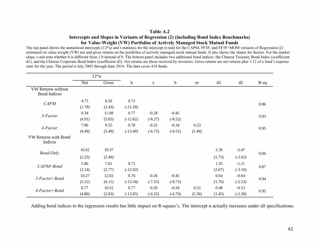
42
Table A.2
Intercepts and Slopes in Variants of Regression (2) (including Bond Index Benchmarks)
for Value-Weight (VW) Portfolios of Actively Managed Stock Mutual Funds The top panel shows the annualized intercepts (12*α) and t-statistics for the intercept (t-stat) for the CAPM, FF3F, and FF3F+MOM versions of Regression (2)
estimated on value-weight (VW) net and gross returns on the portfolios of actively managed stock mutual funds. It also shows the slopes for factors. For the market
slope, t-stat tests whether b is different from 1.0 instead of 0. The bottom panel includes two additional bond indices: the Chinese Treasury Bond Index (coefficient
d1), and the Chinese Corporate Bond Index (coefficient d2). Net returns are those received by investors. Gross returns are net returns plus 1/12 of a fund’s expense
ratio for the year. The period is July 2003 through June 2014. The data cover 418 funds.
Net Gross b s h m d1 d2 R-sq
VW Returns without Bond Indices
4.75 6.50 0.72
(1.78) (2.43) (-11.39)
9.34 11.08 0.77 -0.28 -0.45
(4.91) (5.83) (-12.82) (-8.27) (-8.52)
7.80 9.55 0.78 -0.22 -0.34 0.23
(4.49) (5.49) (-13.40) (-6.75) (-6.52) (5.49)
VW Returns with Bond Indices
16.62 18.37 2.36 -2.47
(2.25) (2.49) (1.73) (-2.62)
5.86 7.61 0.71 1.35 -1.11
(2.14) (2.77) (-12.02) (2.67) (-3.16)
10.27 12.02 0.76 -0.26 -0.45 0.64 -0.64
(5.22) (6.11) (-13.34) (-7.55) (-8.73) (1.76) (-2.53)
8.77 10.52 0.77 -0.20 -0.34 0.22 0.48 -0.53
(4.86) (5.83) (-13.85) (-6.25) (-6.76) (5.36) (1.45) (-2.28)
12*α
CAPM+Bond
0.95
Bond Only 0.06
CAPM
3-Factor
0.86
0.93
0.95
0.87
0.94
4-Factor
3-Factor+Bond
4-Factor+Bond
Adding bond indices to the regression results has little impact on R-square’s. The intercept α actually increases under all specifications.
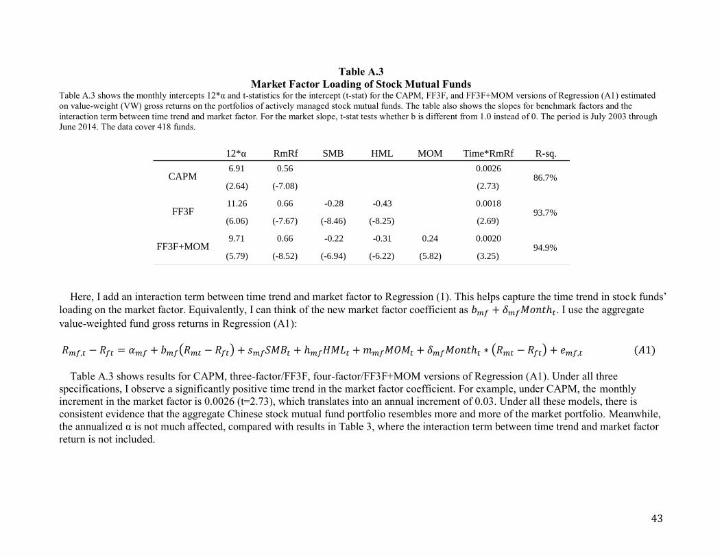
43
Table A.3
Market Factor Loading of Stock Mutual Funds Table A.3 shows the monthly intercepts 12*α and t-statistics for the intercept (t-stat) for the CAPM, FF3F, and FF3F+MOM versions of Regression (A1) estimated
on value-weight (VW) gross returns on the portfolios of actively managed stock mutual funds. The table also shows the slopes for benchmark factors and the
interaction term between time trend and market factor. For the market slope, t-stat tests whether b is different from 1.0 instead of 0. The period is July 2003 through
June 2014. The data cover 418 funds.
12*α RmRf SMB HML MOM Time*RmRf R-sq.
6.91 0.56 0.0026
(2.64) (-7.08) (2.73)
11.26 0.66 -0.28 -0.43 0.0018
(6.06) (-7.67) (-8.46) (-8.25) (2.69)
9.71 0.66 -0.22 -0.31 0.24 0.0020
(5.79) (-8.52) (-6.94) (-6.22) (5.82) (3.25)
CAPM
FF3F
FF3F+MOM
86.7%
93.7%
94.9%
Here, I add an interaction term between time trend and market factor to Regression (1). This helps capture the time trend in stock funds’
loading on the market factor. Equivalently, I can think of the new market factor coefficient as . I use the aggregate
value-weighted fund gross returns in Regression (A1):
Table A.3 shows results for CAPM, three-factor/FF3F, four-factor/FF3F+MOM versions of Regression (A1). Under all three
specifications, I observe a significantly positive time trend in the market factor coefficient. For example, under CAPM, the monthly
increment in the market factor is 0.0026 (t=2.73), which translates into an annual increment of 0.03. Under all these models, there is
consistent evidence that the aggregate Chinese stock mutual fund portfolio resembles more and more of the market portfolio. Meanwhile,
the annualized α is not much affected, compared with results in Table 3, where the interaction term between time trend and market factor
return is not included.

44
B. Cross-Sectional Performance: Bootstrap Simulation
B1. Setup
For my fund sample from 1998 to 2014, I run Regression (1) to estimate each fund’s CAPM,
FF3F, or FF3F+MOM α for net and gross returns. To get zero-α returns, I simply subtract a
fund’s α estimate from all its monthly returns. For example, to compute FF3F zero-α net returns
for a fund, I subtract its estimated FF3F α from the fund’s monthly net returns. Thus, when I run
Regression (1) with the resulting zero-α returns as the dependent variable, I get back a zero
intercept. I calculate zero-α returns for net and gross returns, under CAMP, FF3F and
FF3F+MOM models. The result is 6 populations of zero-α returns.
Setting true α to zero builds different assumptions about skill into the tests on net and gross
fund returns. The zero-α net return sample implies a world where every manager has sufficient
skill that generates expected returns that cover all costs. The zero-α gross return sample
corresponds to a world where every manager has sufficient skill that generates expected returns
that cover costs missed in expense ratios.
A simulation run/pseudo-sample is then generated from bootstrapping with replacement.
There are in total 195 calendar months in my sample period from April 1998 to June 2014. So
the pseudo-sample for all the funds is a random sample (with replacement) of 195 months, drawn
from the 195 calendar months of April 1998 to June 2014. The pseudo-sample is the same
random sample of months, for net and gross returns, under CAPM, FF3F and FF3F+MOM
benchmark models.
For each of the 6 sets of zero-α returns, I estimate, fund by fund, the relevant benchmark
model on the simulation draw of months of zero-α returns, dropping funds that are in the
simulation run for less than 8 months. Funds with less than 8 months of returns in 10,000
pseudo-samples account for less than 0.05%, thus unlikely to affect results. I use zero-α returns
as the dependent variable in Regression (1) and produce cross-sections of α estimates. I do
10,000 simulation runs to produce 6 distributions of t(α), for a world in which true α is zero. I
focus on t(α), rather than α, to control for differences in precision due to differences in residual
variance and in the number of months funds are in a pseudo-sample.
To analyze simulation results, I first compare the percentiles of the cross-section of t(α)
estimates from actual fund returns with the average values of the percentiles from the simulations.
I then look at the likelihood statements to see whether the cross-section of t(α) estimates for
actual fund returns points to the existence of skill.
B2. Comparison of t(α) Percentiles and Cumulative Distribution Function (CDF)
When I estimate a benchmark model on the returns of each fund, I get a cross-section of t(α)
estimates that can be ordered into a cumulative distribution function (CDF) of t(α) estimates for
actual fund returns. A simulation run for the same benchmark model also produces a cross-
section of t(α) estimates and its CDF for a zero-α world. Table B.1, B.2, and B.3 show the CDF
of t(α) estimates for actual returns and the average of the 10,000 simulation CDFs.
Table B.1, B.2, and B.3 respectively report results for CAPM, FF3F and FF3F+MOM model.
First, I compare (i) the values of t(α) at selected percentiles of the CDF of the t(α) estimates from
actual fund returns (Act) and (ii) the averages across the 10,000 simulation runs of the t(α)
estimates at the same percentiles (Sim). Note the average simulated distribution of t(α) is fairly
symmetric and centered around 0. This is not surprising since we simulate from zero-α returns.
The left panel shows results for net returns. Managers seem to have sufficient skill to cover

45
their costs. For all benchmark models, the average simulated t(α) is lower than the actual t(α) for
all percentiles. Under CAPM benchmark model, e.g., the 5th
percentiles of the actual t(α)
estimates −0.59 is larger than the average estimates from the simulation −1.50. The 50th
percentiles of the actual t(α) estimates 1.20 is larger than the average estimates from the
simulation −0.01. The 95th
percentiles of the actual t(α) estimates 3.05 is larger than the average
estimates from the simulation 1.43.
The right panel shows results for gross returns. Not surprisingly, gross returns produce better
actual t(α) estimates. For all benchmark models, the average simulated t(α) is always lower than
the actual t(α) for all percentiles. Clearly, fund managers have sufficient skill to cover costs
missing from expense ratios.
The figure below each table plots the average simulated CDFs and the actual net/gross return
CDFs for t(α). Clearly, under all benchmark models, the actual net return t(α) CDF first order
stochastically dominates (FOSD) the average simulated t(α) CDF. This visual interpretation
offers another perspective for widespread manager skill.
B3. Likelihood Analysis
%<Act column in Table B.1, B.2 and B.3 shows the fraction of the 10,000 simulation runs that
produce lower values of t(α) at the selected percentiles than actual fund returns. These
likelihoods allow me to judge more formally whether the tails of the cross-section of t(α) for
actual fund returns are extreme relative to what we observe when true α is zero.
At the left tail for the worst managers, I infer some managers lack sufficient skill to cover all
costs if %<Act is low, i.e. large fractions of the simulation runs beat the t(α) estimates from
actual net fund returns. The intuition goes the other way too. At the right tail for the best
managers, I infer some managers possess sufficient skill to cover costs if %<Act is high, i.e.
large fractions of the simulation runs are below the t(α) estimates from actual net fund returns. It
is similar for gross fund returns, but the question is whether managers possess sufficient skill to
cover costs missing from expense ratios.
Fama and French (2010) pointed out two issues with likelihood analysis: multiple comparison
and correlation across different likelihoods. To cope with these issues, I will focus on a given
percentile of each tail (5th
and 95th
percentiles) in the following analysis. For example, under
CAPM benchmark model, at 5th
percentile, actual t(α) is −0.59. The likelihood that simulated t(α)
is less than −0.59 out of 10,000 simulations is 97.08%. At 95th
percentile, actual t(α) is 3.05. The
likelihood that simulated t(α) is less than 3.05 out of 10,000 simulation runs is 99.57%. At both
tails, there is dominant evidence for manager skill sufficient to cover costs.
For gross returns, results look better, i.e. there is widespread evidence for manager skill
sufficient to cover costs missing from expense ratios. For example, under CAPM benchmark
model, at 5th
percentile, actual t(α) is −0.28. The likelihood that simulated t(α) is less than −0.28
out of 10,000 simulations is 99.56%. At 95th
percentile, actual t(α) is 3.38. The likelihood that
simulated t(α) is less than 3.38 out of 10,000 simulation runs is 99.88%. At both tails, there is
clear evidence for manager skill sufficient to cover costs missing from expense ratios.

46
Table B.1
Percentiles of t(α) Estimates for Actual and Simulated Fund Returns: Stock Funds
Net/Gross Returns ~ CAPM The table shows values of t(α) at selected percentiles (Pct) of the distribution of t(α) estimates for actual (Act) net
stock fund returns. The table also shows the percent of the 10,000 simulation runs that produce lower values of t(α)
at the selected percentiles than those observed for actual fund returns (%<Act). Sim is the average value of t(α) at
the selected percentiles from the simulations. Sample period is April 1998 to June 2014 and results are shown for the
CAPM. There are 418 stock funds in total.
Stock Funds
Pct Sim Act %<Act Sim Act %<Act
1 -2.25 -1.53 88.33 -2.25 -1.12 98.48
2 -1.93 -1.09 94.53 -1.93 -0.65 99.68
3 -1.74 -0.79 97.41 -1.74 -0.39 99.89
4 -1.61 -0.64 97.74 -1.61 -0.36 99.66
5 -1.50 -0.59 97.08 -1.50 -0.28 99.56
10 -1.15 -0.30 95.77 -1.15 0.02 99.40
20 -0.75 0.14 96.08 -0.75 0.52 99.63
30 -0.47 0.57 97.85 -0.47 0.89 99.66
40 -0.23 0.90 98.56 -0.23 1.24 99.77
50 -0.01 1.20 98.87 -0.01 1.54 99.85
60 0.21 1.43 98.84 0.21 1.80 99.82
70 0.45 1.83 99.30 0.45 2.13 99.82
80 0.72 2.13 99.34 0.72 2.46 99.82
90 1.10 2.59 99.31 1.10 3.00 99.86
95 1.43 3.05 99.57 1.43 3.38 99.88
96 1.52 3.17 99.58 1.52 3.63 99.91
97 1.64 3.41 99.60 1.64 3.78 99.93
98 1.80 3.59 99.57 1.80 4.06 99.91
99 2.08 3.84 99.15 2.08 4.38 99.79
Net Return CAPM Gross Return CAPM

47
Table B.2
Percentiles of t(α) Estimates for Actual and Simulated Fund Returns: Stock Funds
Net/Gross Returns ~ FF3F The table shows values of t(α) at selected percentiles (Pct) of the distribution of t(α) estimates for actual (Act) net
stock fund returns. The table also shows the percent of the 10,000 simulation runs that produce lower values of t(α)
at the selected percentiles than those observed for actual fund returns (%<Act). Sim is the average value of t(α) at
the selected percentiles from the simulations. Sample period is April 1998 to June 2014 and results are shown for the
FF3F model. There are 418 stock funds in total.
Stock Funds
Pct Sim Act %<Act Sim Act %<Act
1 -2.60 -1.63 95.61 -2.60 -1.35 99.21
2 -2.20 -1.35 96.01 -2.20 -1.14 98.96
3 -1.98 -1.22 95.00 -1.98 -0.97 98.98
4 -1.83 -1.12 94.05 -1.82 -0.83 99.03
5 -1.71 -0.97 95.35 -1.70 -0.65 99.53
10 -1.31 -0.41 98.82 -1.31 -0.08 99.96
20 -0.85 0.19 99.58 -0.85 0.46 99.98
30 -0.53 0.60 99.79 -0.53 0.92 99.99
40 -0.27 0.96 99.89 -0.26 1.26 99.99
50 -0.02 1.41 99.99 -0.01 1.71 100.00
60 0.23 1.78 100.00 0.24 2.16 100.00
70 0.50 2.25 100.00 0.51 2.71 100.00
80 0.82 2.74 100.00 0.82 3.24 100.00
90 1.26 3.39 100.00 1.27 3.83 100.00
95 1.64 4.11 100.00 1.66 4.58 100.00
96 1.76 4.24 100.00 1.77 4.75 100.00
97 1.90 4.35 99.99 1.91 4.91 100.00
98 2.11 4.64 99.89 2.12 5.12 99.92
99 2.48 4.75 99.06 2.49 5.26 99.32
Net Return FF3F Gross Return FF3F

48
Table B.3
Percentiles of t(α) Estimates for Actual and Simulated Fund Returns: Stock Funds
Net/Gross Returns ~ FF3F+MOM The table shows values of t(α) at selected percentiles (Pct) of the distribution of t(α) estimates for actual (Act) net
stock fund returns. The table also shows the percent of the 10,000 simulation runs that produce lower values of t(α)
at the selected percentiles than those observed for actual fund returns (%<Act). Sim is the average value of t(α) at
the selected percentiles from the simulations. Sample period is April 1998 to June 2014 and results are shown for the
FF3F model. There are 418 stock funds in total.
Stock Funds
Pct Sim Act %<Act Sim Act %<Act
1 -3.00 -2.01 89.20 -3.00 -1.75 96.38
2 -2.37 -1.66 90.72 -2.37 -1.38 98.21
3 -2.09 -1.49 90.41 -2.08 -1.28 97.12
4 -1.91 -1.33 90.85 -1.91 -1.13 97.43
5 -1.78 -1.23 90.36 -1.78 -0.89 99.29
10 -1.37 -0.65 97.65 -1.36 -0.34 99.94
20 -0.89 -0.11 98.65 -0.89 0.17 99.97
30 -0.56 0.37 99.65 -0.56 0.68 99.99
40 -0.29 0.72 99.78 -0.28 1.04 99.99
50 -0.03 1.20 99.97 -0.03 1.51 100.00
60 0.22 1.63 99.99 0.23 2.04 100.00
70 0.49 2.17 100.00 0.50 2.59 100.00
80 0.81 2.65 100.00 0.82 3.17 100.00
90 1.26 3.32 100.00 1.27 3.78 100.00
95 1.65 3.91 100.00 1.66 4.44 100.00
96 1.77 4.06 99.99 1.78 4.63 100.00
97 1.93 4.26 99.96 1.93 4.78 99.97
98 2.16 4.43 99.64 2.17 4.90 99.68
99 2.69 4.60 96.57 2.69 5.21 97.36
Net Return FF3F+MOM Gross Return FF3F+MOM

49
C. Chinese Institutional Investors’ Aggregate Stock Holding
Table C.1
Characteristics of Stocks Held by Chinese Institutional Investors At the end of each semiannual period from June 30, 2003 to December 31, 2013, I compute both the fraction of the
market capitalization of each stock that is held by the universe of Chinese institutional investors (instmkt%). I
compute the equal-weighted average characteristic scores for quartile portfolios formed based on separate rankings
on instmkt%. To compute the rank score of a given stock on a given characteristic, I sort all stocks separately by
their market capitalization, book-to-market ratio, and momentum at the beginning of each semiannual period. I
assign each stock a rank score on each characteristic, where the rank lies between zero (low) and one (high). For
example, if there are N stocks at the end of a period, I assign the ith-ranked stock (on a particular characteristic) a
rank score of (i-1)/(N-1) for that semiannual period. Finally, I report the time-series average of all measures across
all periods.
instmkt%Size
RankBook-to-
Market RankMomentum
Rank
instmkt%
Quartile 1 (Bottom) 3.90 0.33 0.48 0.47
Quartile 2 14.53 0.44 0.51 0.49
Quartile 3 27.29 0.54 0.53 0.50
Quartile 4 (Top) 51.41 0.69 0.48 0.54
Table C.2
Performance of Stocks Held and Traded by Chinese Institutional Investors
Single Sorted Quartile Portfolios At the end of each semiannual period from 2003Q2 to 2013Q4, I compute the fraction of the market capitalization of
each stock that is held by the universe of Chinese institutional investors (instmkt%). Next, I compute the buy-and-
hold return on the aggregate portfolio of all stocks held by the institutional investors (All Holdings). I also compute
buy-and-hold returns on quartile portfolios, which are formed by rankings on instmkt% (all stocks with zero instmkt%
are excluded). Buy-and-hold returns on holdings portfolios are based on mimicking the aggregate shareholdings of
each stock at the end of each semiannual period.
At the end of each semiannual period, I create a six-month return series following the portfolio formation, for each
of the portfolio discussed above. I appropriately adjust portfolio value weights monthly to create a buy-and-hold
monthly return series for the six months following portfolio formation. Then I paste the six-month return series
together to create a long time series of monthly returns. For each portfolio, I run a regression under CAPM (i.e.
RMRF), three-factor/FF3F, and four-factor/FF3F+MOM models. I report and t( .
α t(α) α t(α) α t(α)
mfmkt%
All Holdings 0.20 (1.13) 0.48 (4.08) 0.41 (3.62)
Quartile 1 (Bottom) 0.01 (0.05) -0.49 (-3.61) -0.51 (-3.75)
Quartile 2 0.02 (0.06) -0.36 (-2.28) -0.34 (-2.13)
Quartile 3 0.16 (1.15) 0.05 (0.40) 0.02 (0.18)
Quartile 4 (Top) 0.19 (0.87) 0.52 (3.99) 0.46 (3.56)
Top-Bottom 0.17 (0.35) 1.01 (4.76) 0.97 (4.51)
CAPM FF3F FF3F+MOM

50
D. Correlations between the Mutual Fund Trading Portfolio and the Insider-Mimicking
Portfolio (CAPM, FF3F)
CAPM specification:
FF3F specification:
Table D
Intercepts and Slopes in Regression (D1) to (D4) Table D shows the monthly intercepts α and t-statistics for the intercept (t-stat) for Regression (D1), (D2), (D3), and
(D4) estimated on returns of the mutual funds’ aggregate trading portfolio. The table also shows the slopes for
factors. For the market slope, t-stat tests whether b is different from 1.0 instead of 0. Top panel shows results for
Regression (D1) and (D2). Bottom panel reports results for Regression (D3) and (D4). Sample period is April 2008
through June 2014, a total of 75 months.
Mutual Fund Trading Portfolio α b s h c R-sq.
0.63 1.08
(1.41) (1.38)
-0.06 1.08 0.58
(-0.15) (1.59) (4.94)
0.79 1.10 -0.04 -0.68
(1.88) (2.04) (-0.34) (-4.89)
0.45 1.10 -0.04 -0.68 0.81
(1.22) (2.39) (-0.39) (-5.72) (5.23)FF3F+Insider 91.9%
CAPM+Insider 88.3%
CAPM 84.3%
FF3F 88.7%
Similar to the FF3F+MOM results in section V subsection A1, here I observe a significant
loading on the insider factor c=0.58 with t=4.94 (under CAPM), and c=0.81 with t=5.23 (under
FF3F). R-square increases after including the insider factor under both models: 84.3% to 88.3%
under CAPM and 88.7% to 91.9% under FF3F. Finally, α decreases substantially after including
the insider factor. It decreases from 0.63 (t=1.41) to 0.06 (t= under CAPM, and from 0.79 (t=1.88) to 0.45 (t=1.22) under FF3F.
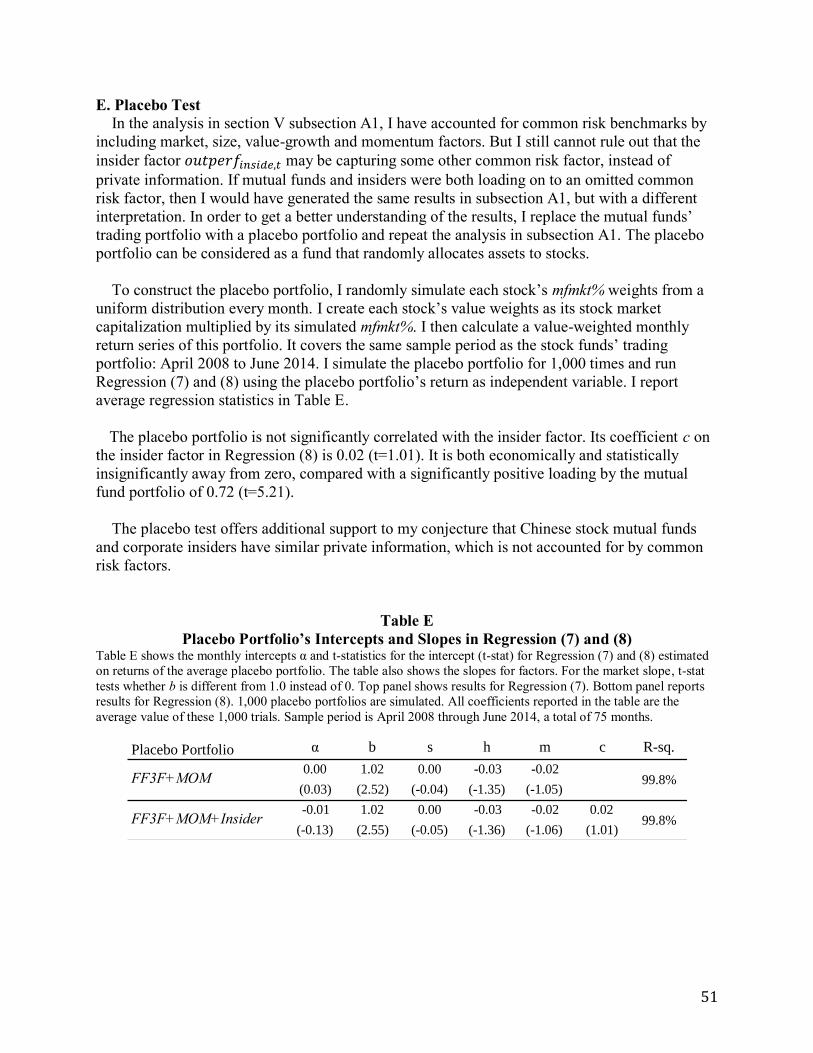
51
E. Placebo Test
In the analysis in section V subsection A1, I have accounted for common risk benchmarks by
including market, size, value-growth and momentum factors. But I still cannot rule out that the
insider factor may be capturing some other common risk factor, instead of
private information. If mutual funds and insiders were both loading on to an omitted common
risk factor, then I would have generated the same results in subsection A1, but with a different
interpretation. In order to get a better understanding of the results, I replace the mutual funds’
trading portfolio with a placebo portfolio and repeat the analysis in subsection A1. The placebo
portfolio can be considered as a fund that randomly allocates assets to stocks.
To construct the placebo portfolio, I randomly simulate each stock’s mfmkt% weights from a
uniform distribution every month. I create each stock’s value weights as its stock market
capitalization multiplied by its simulated mfmkt%. I then calculate a value-weighted monthly
return series of this portfolio. It covers the same sample period as the stock funds’ trading
portfolio: April 2008 to June 2014. I simulate the placebo portfolio for 1,000 times and run
Regression (7) and (8) using the placebo portfolio’s return as independent variable. I report
average regression statistics in Table E.
The placebo portfolio is not significantly correlated with the insider factor. Its coefficient c on
the insider factor in Regression (8) is 0.02 (t=1.01). It is both economically and statistically
insignificantly away from zero, compared with a significantly positive loading by the mutual
fund portfolio of 0.72 (t=5.21).
The placebo test offers additional support to my conjecture that Chinese stock mutual funds
and corporate insiders have similar private information, which is not accounted for by common
risk factors.
Table E
Placebo Portfolio’s Intercepts and Slopes in Regression (7) and (8) Table E shows the monthly intercepts α and t-statistics for the intercept (t-stat) for Regression (7) and (8) estimated
on returns of the average placebo portfolio. The table also shows the slopes for factors. For the market slope, t-stat
tests whether b is different from 1.0 instead of 0. Top panel shows results for Regression (7). Bottom panel reports
results for Regression (8). 1,000 placebo portfolios are simulated. All coefficients reported in the table are the
average value of these 1,000 trials. Sample period is April 2008 through June 2014, a total of 75 months.
Placebo Portfolio α b s h m c R-sq.
0.00 1.02 0.00 -0.03 -0.02
(0.03) (2.52) (-0.04) (-1.35) (-1.05)
-0.01 1.02 0.00 -0.03 -0.02 0.02
(-0.13) (2.55) (-0.05) (-1.36) (-1.06) (1.01)FF3F+MOM+Insider 99.8%
FF3F+MOM 99.8%
Top Related