


Languages
Pages
Legal


MPRAMunich Personal RePEc Archive
Price Comovement Between Biodieseland Natural Gas
Karel Janda and Jakub Kourilek
3 November 2016
Online at https://mpra.ub.uni-muenchen.de/74887/MPRA Paper No. 74887, posted 4 November 2016 00:03 UTC
Price Comovement Between Biodiesel and NaturalGas ∗
Karel Jandaa,b and Jakub Kourileka
aCharles UniversitybUniversity of Economics, Prague
October 28, 2016
Abstract
We study relationship between biodiesel, as a most important biofuel in the EU,
relevant feedstock commodities and fossil fuels. Our main interest is to capture
relationship between biodiesel and natural gas. They are both used either directly
as a fuel or indirectly in form of additives in transport. Therefore, our purpose is to
find price linkage between biofuel and natural gas to support or reject the claim that
they compete as alternative fuels and potential substitutes. The estimated price
link between biodiesel and diesel is negative and the strongest among analysed
commodities. The price transmission between biodiesel and natural gas is the
weakest one.
Keywords: biofuels, shale gas
JEL Codes: Q16, Q42
1 Introduction
We study relationship between biodiesel, as a most important biofuel in the EU, relevant
feedstock commodities and fossil fuels. Our main interest is to capture relationship be-
tween biodiesel and natural gas. They are both used either directly as a fuel or indirectly
∗Email addresses: [email protected] (Karel Janda), [email protected] (JakubKourilek). This project has received funding from the European Union’s Horizon 2020 Research andInnovation Staff Exchange programme under the Marie Sklodowska-Curie grant agreement No 681228.We also acknowledge support from the Czech Science Foundation (grants 15-00036S and 16-00027S)and from University of Economic, Prague (institutional support IP100040). Karel Janda acknowledgesresearch support provided during his long-term visits at Australian National University and McGill Uni-versity. The views expressed in the paper are those of the authors and not necessarily those of ourinstitutions.
1

in form of additives in transport. Therefore, our purpose is to find price linkage between
biofuel and natural gas to support or reject the claim that they compete as alternative
fuels and potential substitutes.
2 Theoretical framework
Biofuel market is subject to substantial regulation in the EU. In fact, regulation creates
biofuel market through indicative or mandatory targets and corresponding incentives such
as blending mandates and production subsidies. Serra et al. (2008) described biofuel
market as standard supply and demand market with technical and regulatory barriers.
They used such framework to study nonlinear price transmission in corn-ethanol-oil price
system in the US. This framework suits the EU biofuel market well. Blending ”wall”
or mandatory blending mandates can be assigned to regulatory constraint. It lays down
minimum quantity of biofuel that has to be placed on the market. On the other hand,
technical constraint represents production limits and technical limits of biofuel application
as a fuel. In actual fact it sets maximum quantity of biofuel that can be put on the
market. We can imagine them as vertical lines in standard economic supply and demand
equilibrium model. These constraints may set such conditions that market equilibrium is
unachievable. For example, when price of relevant fossil fuel decreases, demand for biofuel
shifts which results in lower price and less quantity of biofuel on the market. Supply
function behaves in a similar way when price of relevant feedstock increases, which pushes
biofuel price up. However, technical and regulatory barriers can prevent market from
achieving new equilibrium. Price and quantity are then determined by the barrier which
results in price above the equilibrium price. Moreover, these barriers may vary over time
due to regulation changes or technical innovations. That can cause demand and supply
functions to follow nonlinear patterns in converging to those constraints (Kristoufek et al.,
2014). Further, they claim that, as a cause of constraints, supply and demand functions
2

will rather change their shape than perform horizontal or vertical shifts like in a standard
economic framework. It is another argument for nonlinear nature of supply and demand
which leads to price dependence and co-movements among commodities.
For estimation of price dependences econometrics often uses log-log model. Estimated
coefficient than represents elasticity of one commodity to another. However, if we consider
model of prices in logarithmic form on both sides of an equation:
logPj = α + βlogPi + υ (1)
Estimated coefficient β represent elasticity in form ePj
Pi=
∆Pj/Pj
∆Pi/Pi
. It is not a stan-
dard microeconomic cross-price elasticity which describes how demanded quantity of one
commodity reacts to changes in price of another one. It is defined as eji =∆Qdj/Qdj
∆Pi/Pi
and
it gains positive and negative values which corresponds to their microeconomic relation,
i.e. if they are gross substitutes or gross complements, respectively. However, if we lack
data on demanded quantity the elasticity from log-log model serves as a good substitute.
It is convenient to distinguish between them since both captures different phenomenon.
Thus, we call it price transmission between commodity i and j as Kristoufek et al. (2014)
do. The price transmission represents how price of a commodity j reacts to changes in
price of a commodity i (Kristoufek et al., 2012). In fact, they showed that price trans-
mission is a ratio between own price elasticity of demand and aforementioned cross price
elasticity of demand for a commodity j.
ePj
Pi=
∆Pj/Pj
∆Pi/Pi
=∆Pj/Pj
∆Pi/Pi
× Qdi/∆Qdi
Qdi/∆Qdi
=∆Pj/Pj
∆Qdi/Qdi
× ∆Qdi/Qdi
∆Pi/Pi
=1
ediPj
× ediPi=ediPi
ediPj
(2)
If absolute value of price transmission is less than one, then price of commodity i - Pi
reacts more to the changes in demanded quantity Qdi of commodity i than of commodity j
(Kristoufek et al., 2012). That is what one would expect. To capture introduced possible
3

nonlinearities on biofuel market, we use approach proposed by Kristoufek et al. (2014).
The standard log-log model is extended by expression that capture price dependence to
second order polynomial.
ePiPj
= α + γ1Pi + γ2P2i (3)
Therefore, the model for price transmission between two commodities that allows for
nonlinear relations is stated as follows:
logPj = α + β0logPi + +β1Pi + β2P2i + ε (4)
According to Kristoufek et al. (2014), proposed framework is able to control for
not only price dependence, but also for time dependence which is benefit over standard
constant elasticity approach that assume constant elasticity over time. It enable us to
analyse development of the price transmission between desired commodities over time
and connect it to certain occurrences on market.
3 Data description
Our dataset consists of time series of biodiesel, related fossil fuels and feedstocks prices.
Target market of this work is the EU, thus we analyse biodiesel and closely related com-
modities. In a previous studies German diesel was found to have price link with biodiesel
and it is undoubtedly its close substitute. Further, we include prices of relevant feed-
stocks into our dataset. Rapeseed as the most common used feedstock for production of
biodiesel in the EU and soybeans are included. Besides, we add time series of prices of
Brent crude oil and the UK natural gas. Our dataset contains information on demanded
quantity of some of variables. they turned out to be good instruments within 2SLS es-
timation. Time series range between April 2009 and January 2015. Unfortunately, our
dataset does not contain year 2008 when the food crisis occurred. Since prices of biodiesel
4

are illiquid, we use weekly data for our analysis. Summary statistics are enclosed in the
Appendix. All series were obtained from the Thomson Reuters Contributed Data. Sum-
mary of commodity tickers is presented in Table 1.
Table 1: Analysed commodities
Commodity Ticker Contract type
Biodiesel FAME FOB ARA spot, ARA OTCDiesel ULSD10 spot, ARA FOB
Crude oil BRENT CRUDE JU futures, ICERapeseed RAPESEED EU MA futures, MATIFSoybeans CBT SOYBEANS MAY5 futures, CBOT
Natural gas NAT BAL PT MAY futures, ICE
It is know from previous literature that oil and gas prices and generally series of
prices of energy commodities contain unit roots, i.e. their series are non-stationary and
first-order integrated (Asche et al., 2012). Since presence of unit root in time series can
have substantial effect on statistical inference, we test for it. If time series is found to
be highly persistent , i.e. contains unit root, cointegration analysis have to be used.
However, it is convenient to detrend the series and account for seasonal cycles first,
because trending series can be easily confused with highly persistent series. Appropriate
detrending and seasonal adjustment of the series are not common in related literature
what raises questions about their results (Kristoufek et al., 2014). Data filtering was done
by Stata with use of Butterworth filter. Estimated trend and seasonality can be seen in the
Appendix. We applied ADF, DF-GLS and KPSS tests on detrended series in logarithmic
form thereafter. We also provide test statistics for original series. Null hypothesis of
ADF and DF-GLS is that time series contain unit root. Contrary, KPSS assumes series
stationary under the null. Results are depicted in Table 2. It shows test statistics and
corresponding 5 percent critical values. They differ for original and detrended series,
because we used tests that account for linear trend in case of original series. However,
unit root is not rejected in any of original series even though that applied tests accounted
5

for trend. Only discrepancy comes from KPSS statistic on original series of natural gas
which does not reject trend stationarity. The p-value is greater than 10 percent. Whereas
we apply test on properly detrended series that was purged of seasonality, the results are
straightforward. Unit root is rejected in every series and stationarity is not rejected in
case of the ADF, DF-GLS and KPSS, respectively. Therefore, cointegration technique
can not be used and the OLS or 2SLS, alternatively, is right approach.
Table 2: Tests for unit root
Original series Detrended seriesADF DF-GLS KPSS ADF DF-GLS KPSS
Biodiesel -2.167 -2.293 0.152 -5.049 -3.838 0.0167Natural Gas -2.927 -2.727 0.116 -5.807 -3.620 0.0159
Diesel -1.002 -0.769 0.318 -6.373 -5.812 0.0167Brent -0.616 -0.756 0.343 -6.276 -4.978 0.0177
Rapeseed -2.127 -1.845 0.192 -6.145 -2.362 0.0178Soybean -2.316 -2.369 0.184 -6.192 -2.322 0 .0178
5% critical value -3.410 -2.872 0.146 -2.860 -1.979 0.463
Authors computations in Stata.
4 Econometric model
Here we present our model. The model was build on relevant literature reviewed in pre-
vious sections and available dataset to capture price links between biodiesel and natural
gas. Dependent variable is BiodieselPrice and it occurs in the logarithmic form in the
model. Set of explanatory variables consists of prices of diesel, natural gas, Brent crude
oil, rapeseed and soybean. According to the section 3.1, prices occur as in the logarithmic
form, level form and the second order polynomial. Additionally we used information on
demanded quantity of some of commodities in the 2SLS estimation, because they turned
out to be good instruments. Variables are DieselPrice, NGasPrice, NGasV olume,
BrentPrice, BrentV olume, RapeseedPrice, RapeseedV olume, SoybeanPrice and SoybeanV olume.
The model is stated as follows:
6

logPBt = α +5∑
i=1
βilogPit +5∑
i=1
γiPit +5∑
i=1
δiP2it + ut (5)
where PBt and Pit represents biodiesel price in time t and prices of aforementioned
commodities, respectively. t corresponds to the week, thus t=1,2,...,522 since we have
observations for that number of weeks. The error term ut constitutes of unobserved effects
which are uncorrelated with explanatory variables. We used various estimation methods
to precisely estimate the price transmission between analysed commodities. Applied
approaches are described in the Methodology section.
4.1 Expectation
Based on the previous research, we expect the largest price transmission effect between
biodiesel and diesel, since they are undoubtedly the closest substitutes. Certainly, strong
price transmission is expected among feedstocks as well. Again, such price links were
found before (Kristoufek et al., 2014). However, we expect rapeseed price to have larger
effect than soybean, because it is the most common feedstock for biodiesel in the EU. The
price transmission among biodiesel, crude oil and natural gas is hard to forecast since
their separated effect has not been estimated yet. We think that most of information on
crude oil is contained in diesel prices as well and if our hypothesis of price link between
natural gas and biodiesel is correct, then the price transmission should be very low in
case of crude oil.
5 Methodology
In this section, we present procedures that we used to properly estimate our model. We
provide description for the Prais-Winsten and the 2SLS methods. We continue with de-
scription of the Durbin-Watson test for serial correlation and the Hausman specification
test. Section is based on Wooldridge (2009).
7
5.1 Prais-Winsten
If we find that disturbance in the model follow AR(1) process, i.e. are serially correlated,
OLS inference is no longer valid and we have to correct for it. The Prais-Winsten method
is one of few possibilities how to transform the data to remove the serial correlation. The
AR(1) model of errors can be written as
ut = %ut−1 + et, t = 1, 2, ..., n (6)
where et are serially uncorrelated errors. Let consider model with a single explanatory
variable
yt = α + βxt + ut, t = 1, 2, ..., n (7)
where ut follows process specified in equation 6. Then the Prais-Winsten method
suggests to write model 7 for time period t− 1. Thus for t ≥ 2, we write
yt−1 = α + βxt−1 + ut−1 (8)
yt = α + βxt + ut. (9)
We multiply first equation by % from the equation 6 and subtract it from the second
one afterwards. The idea is to get serially uncorrelated errors et.
yt − %yt−1 = (1− %)α + β(xt − %xt−1) + et, t ≥ 2. (10)
We can rewrite equation as
yt = (1− %)α + βxt + et, t ≥ 2, (11)
where yt and xt are so called quasi-differenced data. By application of this procedure
8
we lose first observation. However, that can be easily fixed by multiplying equation 3.9
for t = 1 by (1 − %2)1/2. It using the fact that V ar(ut) =σ2e
1− %2> σ2
e = V ar(et) where
| % |≤ 1. Therefore, we obtain errors with same variation for first observation as well.
The first observation looks as
y1 = (1− %2)1/2α + βx1 + u1 (12)
where u1 = (1− %2)1/2u1, x1 = (1− %2)1/2x1 and y1 = (1− %2)1/2y1. Variation of the
error in 3.12 is equal to variation of errors in 11, i.e. V ar(u1) = (1 − %2)V ar(u1) = σ2e .
If we use OLS regression on model 11 and add 12 we obtain BLUE estimators of α and
β. Prais-Winsten estimators are example of feasible generalised least squares (FGLS)
estimators. They are asymptotically more efficient than OLS estimators when errors
follow AR(1) process.
5.2 Two Stage Least Squares
When one or more explanatory variables suffer from endogeneity, OLS estimators are
generally inefficient. The 2SLS method mitigates the endogeneity problem and gives us
consistent estimators. Source of the endogenity can be either an omitted variable, an
error-in-variables or simultaneity. Let assume model
y1 = α + β1y2 + β2x+ u (13)
where variable y2 is suspected to be endogenous, i.e. suffer from one of the mentioned
problem. We call such equation structural equation. Consider further that we have
variable z which satisfies these two conditions:
Cov(z, u) = 0;
Cov(z, y2) 6= 0.
The first condition means that z is exogenous in the equation and is also referred to
9
as instrument exogeneity. It means that after the y2 and unobserved effect in the error
u has been controlled for, z has no partial effect on y1. The second condition is referred
to as instrument relevance. It requires that variables have to be related in either positive
or negative way, i.e. it has to have partial effect on the endogenous variable y1 after x
has been controlled for. In other words, coefficient π1 in the following equation has to be
different from zero.
y2 = π0 + π1z + π2x+ v (14)
This equation is called reduced form. The 2SLS procedure then regresses y1 on fitted
values y2 from OLS regression 3.14 and x, in fact y2 is used as instrument for y2. OLS
estimates α, β1 and β2 from regression
y1 = α + β1y2 + β2x+ e (15)
are called 2SLS estimators. The error term e = u+ β1v is uncorrelated both with y2
and x. It is using the fact that suspected correlation of y2 and u is purified in regression
14. The method can be extended to the case with more endogenous variables with at
least same number of exogenous variables.
5.3 Tests
To decide which econometric method suits out data best, we have to apply two crucial
tests. The Durbin-Watson tests for serial correlation and we use it to decide whether we
have to correct for it with Prais-Winsten method. The Haussman specification test helps
us to decide between OLS and 2SLS, i.e. to find out if an endogeneity is present.
The Durbin-Watson tests for AR(1) serial correlation. Its statistic (DW) is based on
the OLS residuals and it is defined as:
10

DW =
n∑t=2
(ut − ut−1)2
n∑t=2
u2t
(16)
The DW statistic is closely related to % from regression of OLS residuals on its lagged
values.
ut = α + %ut−1 + et (17)
Even for small sample sizes, DW statistic is close to
DW ≈ 2(1− %). (18)
The DW distribution is derived under full set of classical linear assumptions. Since %
is predominantly positive, hypothesis are stated as follows,
H0 : % 6= 0 (19)
against alternative
H1 : % > 0. (20)
Therefore, rejection of the null hypothesis requires DW to be statistically less than
two. Since the relation to the % is only approximation, the DW statistic has to be com-
pared with two critical values dU and dL upper and lower, respectively. If DW < dL,
then we choose to reject the null in favour of alternative. If DW > dU , we fail to reject
the null hypothesis of serial correlation. Finally, if the DW statistic lays between upper
and lower critical value, the test is inconclusive.
The Hausman specification test directly compares estimated coefficients from OLS
and 2SLS regression and evaluates whether the differences between them are statistically
significant. Following scheme summarizes consistency of procedures under both hypoth-
esis. Hypothesis are:
11
H0 : difference in coefficients is not systematic
H1 : difference in coefficients is systematic
H0 H1
OLS consistent & efficient inconsistent
2SLS consistent consistent
If we reject H0, we choose 2SLS. However, if we fail to reject H0, we choose OLS since
it is more efficient than 2SLS.
6 Results
Since we confirmed the data does not contain unit roots, thus cointegration analysis is
not valid approach and we applied OLS estimation. The Breusch-pagan test confirmed
presence of heteroskedasticity with chi-square statistic χ2 = 108.51 with p-value practi-
cally zero. Therefore, we accounted for it by using heteroskedasticity robust standard
errors. We verified assumption about serial correlation then. The Durbin-Watson test
produced statistic DW = 1.105. Lower critical value for 1 percent significance level is
1.691. Consequently, we concluded that our errors follow AR(1) process and we had to
use the FGLS estimation, since the usual OLS inference is no longer valid under presence
of serially correlated errors. More precisely, we used the Prais-Winsten method that ac-
counts for the first observation and makes the FGLS more efficient in finite sample sizes.
We estimated the model by the 2SLS procedure and we used serial correlation robust
standard errors to account for the serial correlation. The Hausman specification test
yielded statistic 9.65 which corresponds to p-value 0.29. Thus, we chose to not reject the
H0 which means that there is not enough evidence for presence of endogeneity and Prais-
Winsten procedure is consistent. Estimated regressions are depicted in the Appendix.
We left only significant variables in the final model. The model meets assumptions. We
accounted for time trend and seasonalities. Serial correlation of errors is corrected by the
FGLS estimation and we control for heteroskedasticity by using robust standard errors.
12
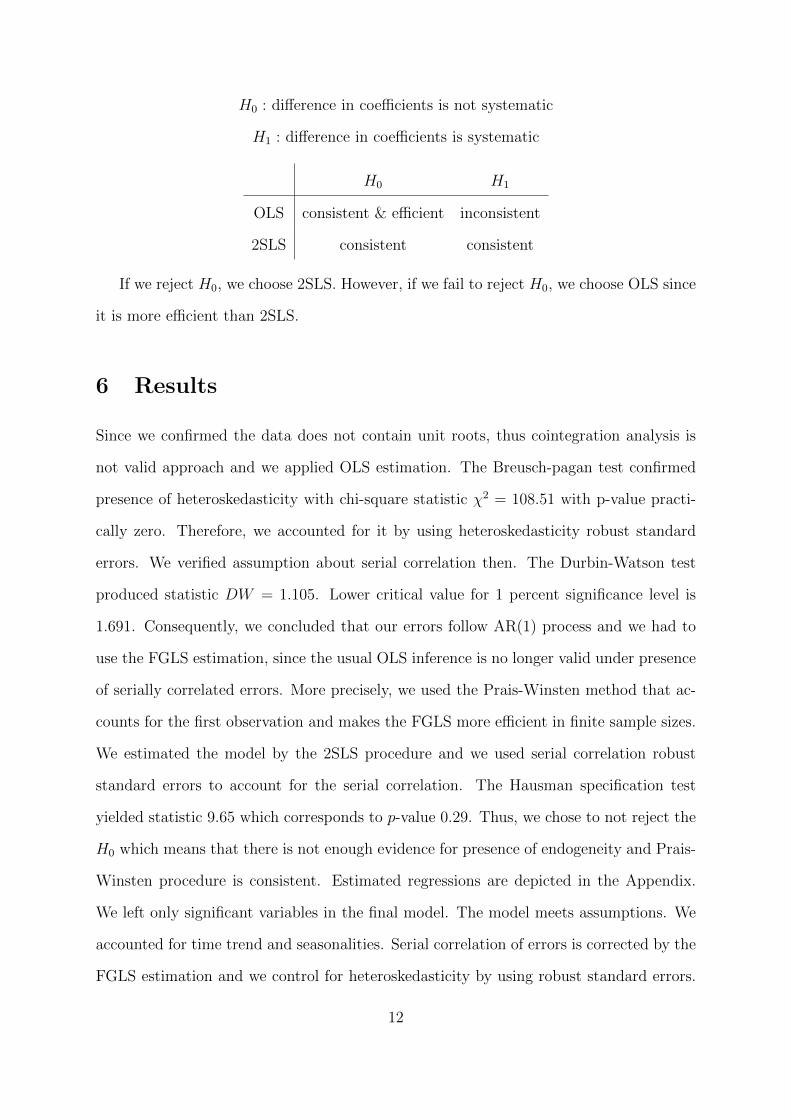
The model is by definition linear in parameters. The R2 = 0.2865 which means that the
model explains 29 percent of the variation in the data.
The model predicts that largest price transmission pertains to diesel. According to
the model, the price-dependent transmission between biodiesel and diesel is linear and for
our data on price of diesel, which ranges between $447 and $1075, the price-dependent
transmission reaches almost -2 for the the highest prices. Estimated price transmission
for soybeans and rapeseed is comparable. It ranges between 0.6 and 1.3 for both com-
modities. The estimate for natural gas is still statistically significant with p-value 0.036.
The price transmission between biodiesel and natural gas is predicted to be the lowest
among analysed commodities. However, is reaches -0.3 for higher prices of natural gas
which can be considered economically significant as well.
Figure 1: Estimated price-dependent price transmission with 95%confidence boundaries
Authors computations.
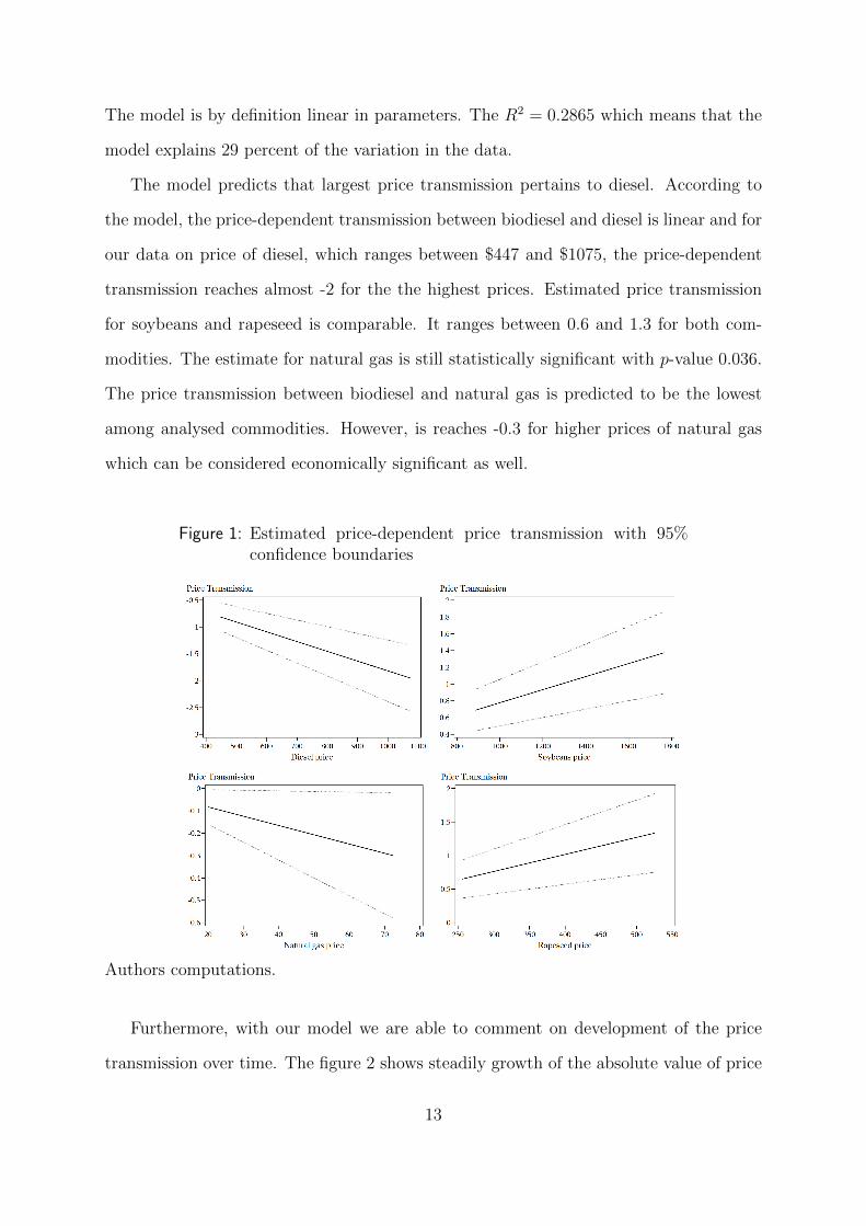
Furthermore, with our model we are able to comment on development of the price
transmission over time. The figure 2 shows steadily growth of the absolute value of price
13

transmission for the biodiesel-diesel pair from 0.8 and peaks approximately at 2 in the
first half of 2011. The following years are represented by fluctuations between values 1.5
and 2. The effect plummets sharply at the end of 2014 when oil prices dropped. The
development of the price transmission over time among soybeans, rapeseed and biodiesel
is again comparable. Their development can be described by three spikes in 2011, than in
summer of 2012 and last in the first half of 2014. Most of the time the price transmission
stays around value 1, however in the end of a tracked period it substantially dropped in
case of soybeans and followed by resurgence in case of rapeseed. We present development
for natural gas price transmission as well, even thought it attains much lower magnitude.
We again present it in absolute value since the relation is estimated to be negative.
The relation gradually grows from 2009 with fluctuations around its trend. It decreases
sharply in 2014 together with price of natural gas.
Figure 2: Development of the price transmission over time with 95%confidence boundaries
Authors computations.
14

7 Conclusions
The estimated price link between biodiesel and diesel is negative and the strongest among
analysed commodities. While we expected strong relation within this pair, the negative
price link is opposed to previous studies. The positive relation was quantified between
German biodiesel and diesel. However, we use different time series in our work. Our
dataset contains time series for ARA biodiesel and diesel. Their prices are created by
trading in three ports the Antwerp, the Rotterdam and the Amsterdam. It suggests that
prices of our commodities have different mutual responsiveness than German consumer
biodiesel and diesel. The price transmission represents how price of one commodity
reacts to changes in price of another. According to results, if price of diesel increases,
the price of biodiesel decreases. Therefore, we can refer to them as so called ”price
substitutes.” Another explanation can be that commodities in ports yield to speculations.
The relation with soybeans and rapeseed price is strong as we expected. Again, the price
transmission is estimated in different direction in case of soybeans price compared to
the previous studies. However, according to the results when price of corresponding
feedstock rises, the price of biodiesel rises as well. This is what one could expect. The
price transmission between biodiesel and natural gas is the weakest one. We can still
denote it as significant. Their relation is negative similar to the diesel, however in a much
smaller size. From the figure 2 we see that the price transmission gradually grows over
5 years. Since, introduction of different technologies into transportation takes a while,
the price transmission would rise gradually rather in a long term. That is in conformity
with the fact that natural gas as an alternative fuel has experienced boom only recently,
thus our dataset may not capture such phenomenon so far. However, we think that as
the number of NGVs and consequently consumption of natural gas based fuels will grow,
the price link may strengthen in a long term.
15

References
[1] KRISTOUFEK, L., K. JANDA a D. ZILBERMAN. Mutual Responsiveness of Biofu-
els, Fuels and Food Prices. Crawford School of Public Policy, The Australian National
University: CAMA Working Papers, 2012. Dostupne z: https://ideas.repec.
org/p/een/camaaa/2012-38.html
[2] KRISTOUFEK, Ladislav, Karel JANDA a David ZILBERMAN. Price transmission
between biofuels, fuels, and food commodities. Biofuels, Bioproducts and Biorefining
[online]. 2014, vol. 8, issue 3, s. 362-373 [cit. 2015-05-12]. DOI: 10.1002/bbb.1464.
Dostupne z: http://doi.wiley.com/10.1002/bbb.1464
[3] SERRA, Teresa, David ZILBERMAN, Jose Maria GIL a Barry K. GOODWIN. Non-
linearities in the US corn-ethanol-oil price system. American Agricultural Economics
Association, 2008. Dostupne z: http://ageconsearch.umn.edu/handle/6512
[4] WOOLDRIDGE, Jeffrey M. Introductory econometrics: a modern approach. 4th ed.
Mason, OH: South Western, Cengage Learning, c2009, xx, 865 p. ISBN 03-246-6054-
5.
[5] ASCHE, Frank, Atle OGLEND a Petter OSMUNDSEN. Gas versus oil prices
the impact of shale gas. Energy policy [online]. 2012, c. 47, s. 117-124 [cit.
2015-03-27]. Dostupne z: http://www.sciencedirect.com/science/article/
pii/S0301421512003382
16

8 Appendix – Tables
Table 3: Summary statistics
Variable Mean Std. Dev. Min. Max. NBiodieselPrice 278.212 108.044 87.5 535 302DieselPrice 840.950 162.667 447.75 1075.5 302NGasPrice 51.77 13.645 20.1 72.38 302NGasVolume 37316.142 17378.408 9325 94160 302BrentPrice 97.455 18.472 50.11 126.65 302BrentVolume 831664.036 229455.232 246497 1476185 302RapeseedPrice 393.383 73.932 255.75 525.25 302RapeseedVolume 14909.235 6771.067 2525 36841 302SoybeanPrice 1264.598 206.616 885 1764.5 302SoybeanVolume 293426.642 224660.41 401 914977 302
Authors computations in Stata.
17

Table 4: OLS Estimation
Variable Coefficient (Std. Err.)log(Diesel) -3.66063† (2.07831)log(NaturalGas) 0.37457 (0.28929)log(Brent) 3.64236∗ (1.80789)log(Rapeseed) 3.44126∗∗ (1.08391)log(Soybean) -1.76576† (1.04036)Diesel 0.00255 (0.00260)NaturalGas -0.01668∗ (0.00680)Brent -0.04039∗ (0.01862)Rapeseed -0.00556∗ (0.00265)Soybean 0.00223∗ (0.00088)NaturalGas2 -0.00015 (0.00039)Brent2 -0.00024 (0.00051)Diesel2 0.00001 (0.00001)Rapeseed2 -0.00002 (0.00002)Soybean2 0.00000 (0.00000)Intercept -0.00219 (0.01050)
N 302R2 0.54935F (15,286) 33.29298Significance levels : † : 10% ∗ : 5% ∗∗ : 1%
Authors computations in Stata.
18

Table 5: 2SLS Estimation
Variable Coefficient (Std. Err.)log(Diesel) 0.70005 (0.73333)Diesel -0.00308 (0.00093)Diesel2 0.00001 (0.00000)log(NaturalGas) 0.12306 (0.30967)log(Rapeseed) 4.04527 (1.28732)log(Soybean) -1.97956 (1.04493)NaturalGas -0.01013 (0.00711)Rapeseed -0.00710 (0.00324)Soybean 0.00239 (0.00084)NaturalGas2 -0.00031 (0.00048)Rapeseed2 -0.00002 (0.00002)Soybean2 0.00000 (0.00000)Intercept 0.00354 (0.01335)
N 302R2 0.53658F (12,.) 20.21911Significance levels : † : 10% ∗ : 5% ∗∗ : 1%
Authors computations in Stata.
Table 6: Prais-Winsten Estimation
Variable Coefficient (Std. Err.)Diesel -0.00182∗∗ (0.00029)NaturalGas -0.00414∗ (0.00196)Rapeseed 0.00254∗∗ (0.00057)Soybean 0.00078∗∗ (0.00014)Intercept -0.00115 (0.01214)
N 302R2 0.2865F (4,297) 18.62163Significance levels : † : 10% ∗ : 5% ∗∗ : 1%
Authors computations in Stata.
19

Figure 3: Log-prices vs. trend and seasonality
Authors computations.
20
Top Related