


Languages
Pages
Legal


Prestack Migration Prestack Migration DeconvolutionDeconvolution
Jianxing Hu and Gerard T. SchusterUniversity of Utah

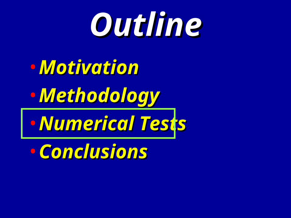
OutlineOutline• MotivationMotivation
• MethodologyMethodology
• Numerical TestsNumerical Tests
• ConclusionsConclusions

Comparison of Poststack MD Depth SlicesComparison of Poststack MD Depth Slices
66
88
Y
(k
m)
Y (
km
)
X (km)X (km)44 88 66 1010
Kirchhoff Kirchhoff ImageImage
MD ImageMD Image
66
88
Y
(k
m)
Y (
km
)
X (km)X (km)44 88 66 1010

Comparison of Prestack Migration and MD ImagesComparison of Prestack Migration and MD Images X (km)X (km) 44 66 88 1010
11
44
D
e pth
(km
)D
epth
(km
)
X (km)X (km) 44 66 88 1010 11
44
D
e pth
(km
)D
epth
(km
)
Prestack Kirchhoff Prestack Kirchhoff Migration Image of Migration Image of
a North Sea Data Seta North Sea Data Set
MD Image
OutlineOutline• MotivationMotivation
• MethodologyMethodology
• Numerical TestsNumerical Tests
• ConclusionsConclusions

Modeling and MigrationModeling and Migration
oosoogsg rdSrRrrGrrGrrd
)()(),(),(),(
drdrdrrdrrGrrGSrm sgsgsg
),(),(),()()( ***
Seismic dataSeismic data ReflectivityReflectivityGreen’s FunctionGreen’s Function
Model SpaceModel Space
Migrated ImageMigrated Image
Data SpaceData Space
Seismic DataSeismic Data
Forward Modeling:Forward Modeling:
Migration:Migration:
WaveletWavelet

ooomig rdrRrrrm
)()()( Model SpaceModel Space
),(),()()()( *** sgomig rrGrrGSSrrWhere:Where:
)( omig rr
Denote Denote as the migration Green’s Functionas the migration Green’s Function
drdrdrrGrrG sgsoog
),(),(
Relation of Migrated Image and Relation of Migrated Image and Reflectivity DistributionReflectivity Distribution
Data SpaceData Space

Reflectivity Modulated Reflectivity Modulated by Migration Green’s Functionby Migration Green’s Function
ooomig rdrRrrrm
)()()(
)(rm
)( omig rr
)( orR
Model SpaceModel Space

Migration DeconvolutionMigration Deconvolution
),,,,( oppoomig zyxzyyxx
oooooo dzdydxzyxR ),,(Model Space
ooomig rdrRrrrm
)()()( Model SpaceModel Space
),( pp yx --- --- reference position of migration Green’s functionreference position of migration Green’s function
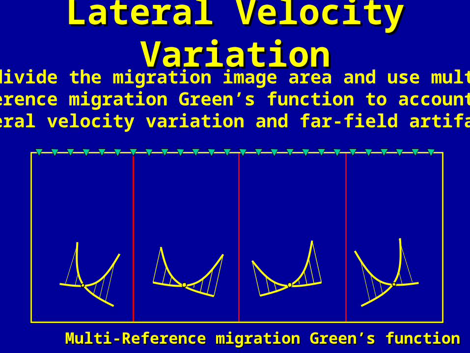
Lateral Velocity VariationLateral Velocity Variation
Multi-Reference migration Green’s functionMulti-Reference migration Green’s function
Subdivide the migration image area and use multi-reference migration Green’s function to account for lateral velocity variation and far-field artifacts
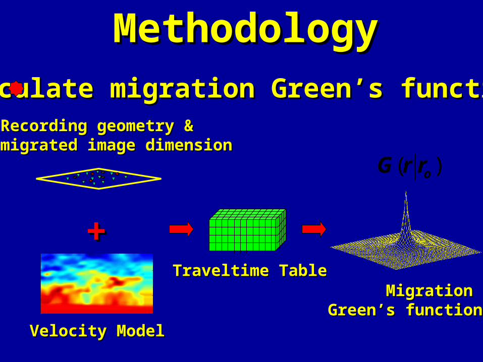
MethodologyMethodology
Calculate migration Green’s function Calculate migration Green’s function Recording geometry &Recording geometry &migrated image dimensionmigrated image dimension
Velocity ModelVelocity Model
++Traveltime TableTraveltime Table
Migration Migration Green’s functionGreen’s function
)( orrG
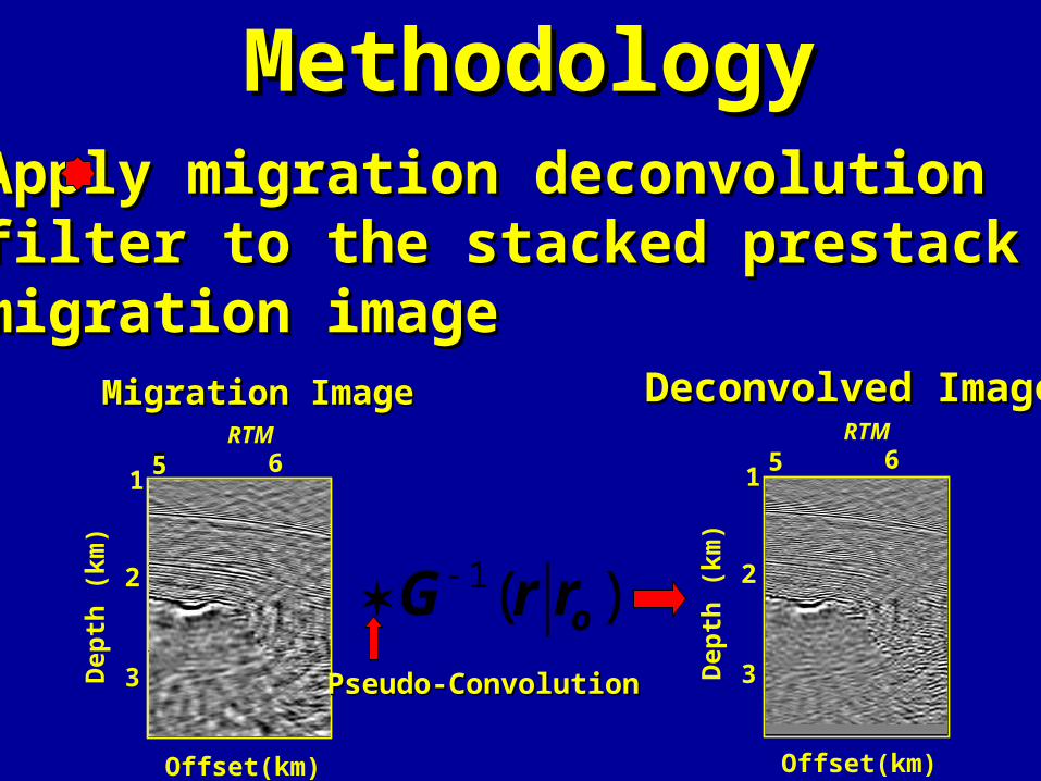
MethodologyMethodologyApply migration deconvolution Apply migration deconvolution filter to the stacked prestack filter to the stacked prestack migration imagemigration image
5
Offset(km)
651
2
3
Dep
th (
km)
RTM
)(1orrG
Migration ImageMigration Image
Deconvolved ImageDeconvolved Image
Pseudo-ConvolutionPseudo-Convolution
Offset(km)
651
2
3
Dep
th (
km)
RTM
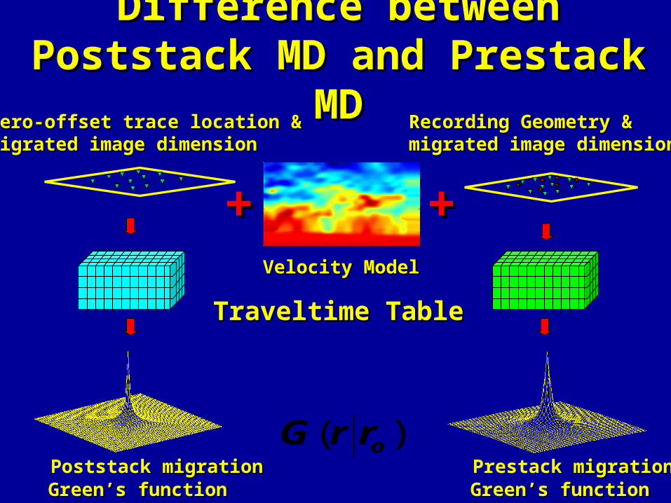
Difference between Poststack MD Difference between Poststack MD and Prestack MDand Prestack MD
Zero-offset trace location &Zero-offset trace location &migrated image dimensionmigrated image dimension
Velocity ModelVelocity Model
Traveltime TableTraveltime Table
Poststack migration migration Green’s functionGreen’s function
)( orrG
++
Prestack migration migration Green’s functionGreen’s function
Recording Geometry &Recording Geometry &migrated image dimensionmigrated image dimension
++
OutlineOutline• MotivationMotivation
• MethodologyMethodology
• Numerical TestsNumerical Tests
• ConclusionsConclusions

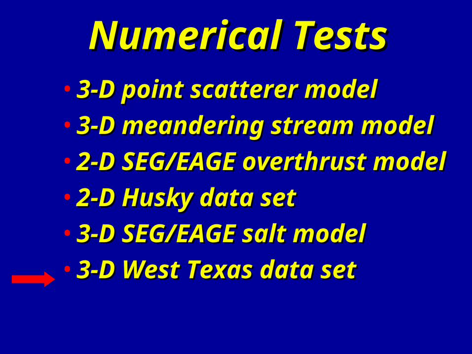
Numerical TestsNumerical Tests• 3-D point scatterer model3-D point scatterer model
• 3-D meandering stream model3-D meandering stream model
• 2-D SEG/EAGE overthrust model2-D SEG/EAGE overthrust model
• 2-D Husky data set (Canadian 2-D Husky data set (Canadian Foothills)Foothills)
• 3-D SEG/EAGE salt model 3-D SEG/EAGE salt model
• 3-D West Texas data set3-D West Texas data set

5 X 5 Sources; 21 X 21 Receivers5 X 5 Sources; 21 X 21 Receivers
(0, 0)(0, 0)
(1km, 0)(1km, 0)
(1km, 1km)(1km, 1km)
(0, 1km)(0, 1km)
Point scattererPoint scatterer
Recording Geometry
kmzyx ooo )7.0,5.0,5.0(
Wavelet frequency 50 Hz

Prestack KM vs. Prestack MDPrestack KM vs. Prestack MD
ozz ozz
dzzz o dzzz o
Y
X
Y
X
Y
X
Y
X

Prestack KM vs. Poststack MDPrestack KM vs. Poststack MD
ozz
dzzz o
Y
X
Y
X
ozz
dzzz o Y
X
Y
X

Numerical TestsNumerical Tests• 3-D point scatterer model3-D point scatterer model
• 3-D meandering stream model3-D meandering stream model
• 2-D SEG/EAGE overthrust model2-D SEG/EAGE overthrust model
• 2-D Husky data set (Canadian 2-D Husky data set (Canadian Foothills)Foothills)
• 3-D SEG/EAGE salt model 3-D SEG/EAGE salt model
• 3-D West Texas data set3-D West Texas data set
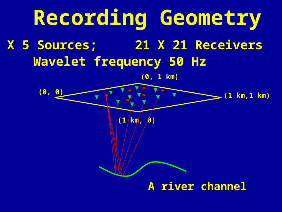
(0, 0)(0, 0)
(1 km, 0)(1 km, 0)
(1 km,1 km)(1 km,1 km)
(0, 1 km)(0, 1 km)
A river channelA river channel
Recording Geometry5 X 5 Sources; 21 X 21 Receivers5 X 5 Sources; 21 X 21 ReceiversWavelet frequency 50 Hz
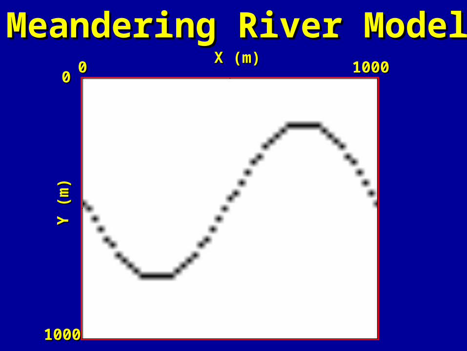
Meandering River ModelMeandering River Model00 10001000
X (m)X (m)00
10001000
Y (
m)
Y (
m)
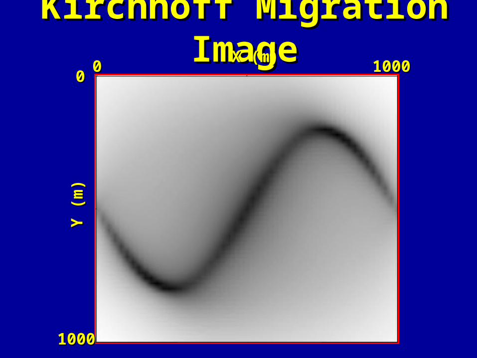
Kirchhoff Migration ImageKirchhoff Migration Image00 10001000
X (m)X (m)00
10001000
Y (
m)
Y (
m)

MD ImageMD Image00 10001000
X (m)X (m)00
10001000
Y (
m)
Y (
m)

Numerical TestsNumerical Tests• 3-D point scatterer model3-D point scatterer model
• 3-D meandering stream model3-D meandering stream model
• 2-D SEG/EAGE overthrust model2-D SEG/EAGE overthrust model
• 2-D Husky data set (Canadian 2-D Husky data set (Canadian Foothills)Foothills)
• 3-D SEG/EAGE salt model 3-D SEG/EAGE salt model
• 3-D West Texas data set3-D West Texas data set

Prestack Migration ImagePrestack Migration Image
Deconvolved Migration ImageDeconvolved Migration Image
0 km0 km 20 km20 km0 km0 km
4 km4 km
20 km20 km 0 km0 km0 km0 km
4 km4 km
X(km)
X(km)
Dep
th (
km
)D
epth
(k
m)

Zoom View of KM and MDZoom View of KM and MD
Prestack KMPrestack KM
Prestack MDPrestack MD
22
44
33
Dep
th (
km
)D
epth
(k
m)
33 77X (km)X (km)
22
44
33
Dep
th (
km
)D
epth
(k
m)
33 77X (km)X (km)

Numerical TestsNumerical Tests• 3-D point scatterer model3-D point scatterer model
• 3-D meandering stream model3-D meandering stream model
• 2-D SEG/EAGE overthrust model2-D SEG/EAGE overthrust model
• 2-D Husky data set (Canadian 2-D Husky data set (Canadian Foothills)Foothills)
• 3-D SEG/EAGE salt model 3-D SEG/EAGE salt model
• 3-D West Texas data set3-D West Texas data set

Husky Prestack Migration ImageHusky Prestack Migration Image
44
66
X(km)X(km)00
00 101055
22
Dep
th (
km
)D
epth
(k
m)

Velocity Model for Husky DataVelocity Model for Husky Data
66
X(km)X(km)00
00 101055
22
Dep
th (
km
)D
epth
(k
m)
70007000
32003200
Vel
ocit
y (m
/s)

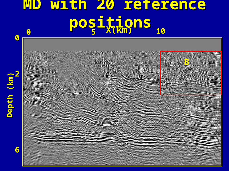
MD with 20 reference positionsMD with 20 reference positions
66
X(km)X(km)00
00 101055
22
Dep
th (
km
)D
epth
(k
m)
AA

KMKM
X(km) 951
3
Dep
th (
km
)
MDMD
X(km) 951
3
Dep
th (
km
)
MD with 20 reference positionsMD with 20 reference positions
66
X(km)X(km)00
00 101055
22
Dep
th (
km
)D
epth
(k
m)
BB

KMKM
X(km) 1411
1
3
Dep
th (
km
)
MDMD
X(km) 1411
1
3
Dep
th (
km
)

MD with 20 reference positionsMD with 20 reference positions
66
X(km)X(km)00
00 101055
22
Dep
th (
km
)D
epth
(k
m)
CC

KMKM
X(km) 14102
5
Dep
th (
km
)
MDMD
X(km) 14102
5
Dep
th (
km
)

Numerical TestsNumerical Tests• 3-D point scatterer model3-D point scatterer model
• 3-D meandering stream model3-D meandering stream model
• 2-D SEG/EAGE overthrust model2-D SEG/EAGE overthrust model
• 2-D Husky data set2-D Husky data set
• 3-D SEG/EAGE salt model 3-D SEG/EAGE salt model
• 3-D West Texas data set3-D West Texas data set

KM Inline (97,Y) SectionKM Inline (97,Y) Section MD Inline (97,Y) SectionMD Inline (97,Y) Section
55 88Y (km)Y (km) 55 88Y (km)Y (km)00
44
22
00
44
22
Dep
th (
km
)D
epth
(k
m)

KM Crossline (X,97) SectionKM Crossline (X,97) Section MD Crossline (X,97) SectionMD Crossline (X,97) Section
00
44
22
Dep
th (
km
)D
epth
(k
m)118
X (km)118
X (km)
00
44
22
Numerical TestsNumerical Tests• 3-D point scatterer model3-D point scatterer model
• 3-D meandering stream model3-D meandering stream model
• 2-D SEG/EAGE overthrust model2-D SEG/EAGE overthrust model
• 2-D Husky data set2-D Husky data set
• 3-D SEG/EAGE salt model 3-D SEG/EAGE salt model
• 3-D West Texas data set3-D West Texas data set
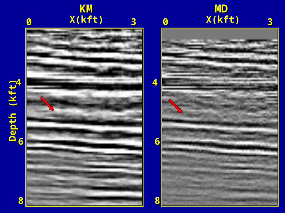
KMKM MDMD00 33X(kft)
44
66
88
Dep
th (
kft
)D
epth
(k
ft) 44
66
88
00 33X(kft)
44
66
88
Dep
th (
kft
)D
epth
(k
ft)
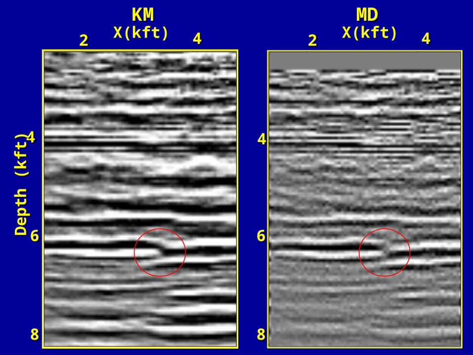
KMKM MDMD
44
66
88
X(kft)22 44X(kft)22 44

OutlineOutline• MotivationMotivation
• MethodologyMethodology
• Numerical TestsNumerical Tests
• ConclusionsConclusions
ConclusionsConclusionsWorks well on 2-D land and 3-D Works well on 2-D land and 3-D synthetic marine prestack data synthetic marine prestack data
More work is needed to remedy More work is needed to remedy the problems in MD for 3-D the problems in MD for 3-D land prestack dataland prestack data
Standard post-migration processing procedure ?

AcknowledgementAcknowledgement• Thank 1999 UTAM sponsors for Thank 1999 UTAM sponsors for
their financial supporttheir financial support
Top Related