


Languages
Pages
Legal


Copyright © 2006, SAS Institute Inc. All rights reserved.
Predictive Modeling with SAS (for Health)
Lorne Rothman, PhD, P.Stat.Principal Analytics Services

Copyright © 2006, SAS Institute Inc. All rights reserved.
Overview
What is Predictive Modeling? Purpose, challenges, and methods
Examples
The North Carolina Low Birth Weight Data
Data & Variable Preparation Oversampling, Missing Values, Data splitting & dimension
reduction
Binary Target Modeling Decision Trees with HPSPLIT
Logistic Regression with LOGISTIC
Comparing ROC curves
Continuous Target Modeling Model selection with GLMSELECT
Generalized Linear Predictive Modeling Gamma regression model selection with HPGENSELECT

Copyright © 2006, SAS Institute Inc. All rights reserved.
What is Predictive Modeling?

Copyright © 2006, SAS Institute Inc. All rights reserved.
Purpose of Predictive Modeling
To Predict the Future
x To identify statistically significant attributes or
risk factors
x To publish findings in Science, Nature, or the
New England Journal of Medicine
To enhance & enable rapid decision making at
the level of the individual patient, client,
customer, etc.
x To enable decision making and influence policy
through publications and presentations

Copyright © 2006, SAS Institute Inc. All rights reserved.
Data Deluge

Copyright © 2006, SAS Institute Inc. All rights reserved.
OK
Rare Condition
Challenges: Rare Events

Copyright © 2006, SAS Institute Inc. All rights reserved.
Methodology: Empirical Validation
Copyright © 2006, SAS Institute Inc. All rights reserved.
Training
Validation
2000 2001
TEST
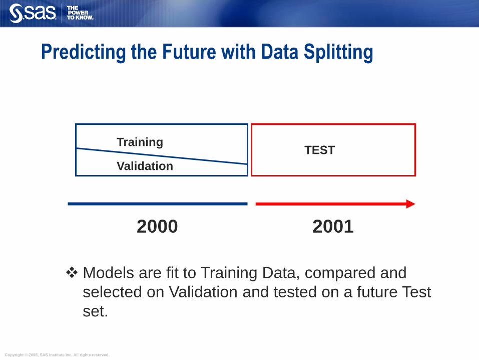
Predicting the Future with Data Splitting
Models are fit to Training Data, compared and
selected on Validation and tested on a future Test
set.
Copyright © 2006, SAS Institute Inc. All rights reserved.
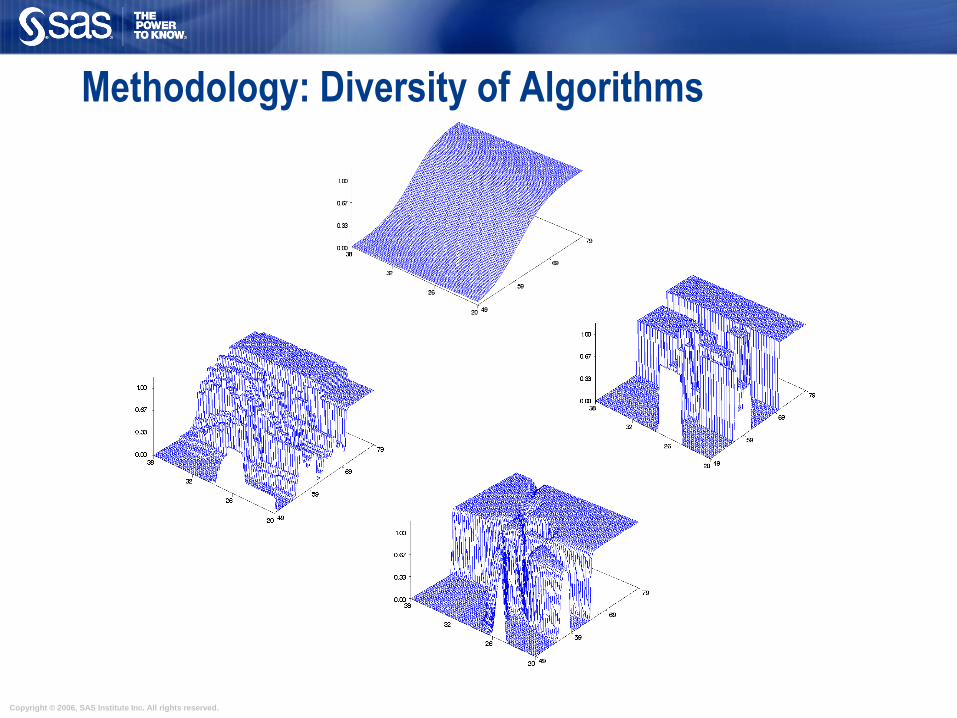
Methodology: Diversity of Algorithms

Copyright © 2006, SAS Institute Inc. All rights reserved.
Jargon… Target = Dependent Variable.
Inputs, Predictors = Independent Variables.
Supervised Classification = Predicting class membership with
algorithms that use a target.
Scoring = The process of generating predictions on new data
for decision making. This is not a re-running of models but an
application of model results (e.g. equation and parameter
estimates) to new data.
Scoring Code = programming code that can be used to
prepare and generate predictions on new data including
transformations, imputation results, and model parameter
estimates and equations.

Copyright © 2006, SAS Institute Inc. All rights reserved.
Examples…
SAS Discharge Disposition and Length of Stay Modeling for Hospitals
Length of stay: Survival modeling to predict ‘target’ discharge date up to 2 days prior to
discharge for patients who end up going home with care or without care.
Discharge disposition: Predict discharge disposition 2 days prior to patient discharge
for those patients who will go home with home care and those who will go home without
homecare.
Data: Use daily in-hospital data from admissions, OR, DI, pharmacy, lab tests, etc. to
score patients daily.
Predicting End Stage Renal Failure
Survival modeling to predict probability of developing End Stage Renal Disease given
patient attributes and kidney function measures.
What makes these predictive models?
Same algorithms as employed in inferential statistics, but different methodology and
modeling purpose—to score individuals in near real time and use results for rapid
and preemptive decision making.
Copyright © 2006, SAS Institute Inc. All rights reserved.
The North Carolina Birth Records Data
North Carolina Birth Records from North Carolina
Center for Health Statistics: 122,550 from 2000, and
120,300 from 2001.
7.2% low birth weight births ( < 2500 grams) excluding
multiple births.
Data contains information on parents ethnicity, age,
education level and marital status.
Data contains information on mothers health condition
and reproductive history.
45 potential predictor variables for modeling.

Copyright © 2006, SAS Institute Inc. All rights reserved.
PREDICTORS
• Parent socio-,eco-, demo- graphics, health and behaviour
•Age, edu, race, medical conditions, smoking, drinking etc.
•Prior pregnancy related data
•# pregnancies, last outcome, prior pregnancies etc.
•Medical History for pregnancy
•Hypertension during pregnancy, eclampsia, incompetent cervix,
etc.
•Obstetric procedures
•Amniocentesis, ultrasound, etc.
•Events of Labor
•Breech, fetal distress etc.
•Method of delivery
•Vaginal, c-section etc.
•New born characteristics
•congenital anomalies (spinabifida, heart), APGAR score, anemia
Scenario: Early Warning System for Birth Weight
Copyright © 2006, SAS Institute Inc. All rights reserved.
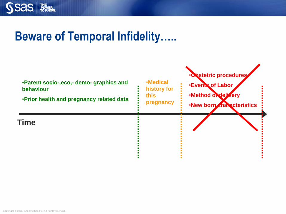
•Parent socio-,eco,- demo- graphics and
behaviour
•Prior health and pregnancy related data
•Obstetric procedures
•Events of Labor
•Method of delivery
•New born characteristics
Time
Beware of Temporal Infidelity…..
•Medical
history for
this
pregnancy

Copyright © 2006, SAS Institute Inc. All rights reserved.
Data & Variable Preparation

Copyright © 2006, SAS Institute Inc. All rights reserved.
1
time
time range
start
date
end
date
target
date
attributes latency period
0Tmaxrelative time
target window
Preparing the Modeling Data

Copyright © 2006, SAS Institute Inc. All rights reserved.
Oversample Rare Events
SURVEYSELECT is used to sample 7.5% of non-events and 100% of events.
Data must be sorted by the target prior to oversampling.

Copyright © 2006, SAS Institute Inc. All rights reserved.
Create Missing Indicators
Create missing indicators to capture associations between missingness and
the target in development data.
The process is repeated for Test data.
This step is unnecessary for Decision Trees as they accommodate missing
values directly.
Copyright © 2006, SAS Institute Inc. All rights reserved.
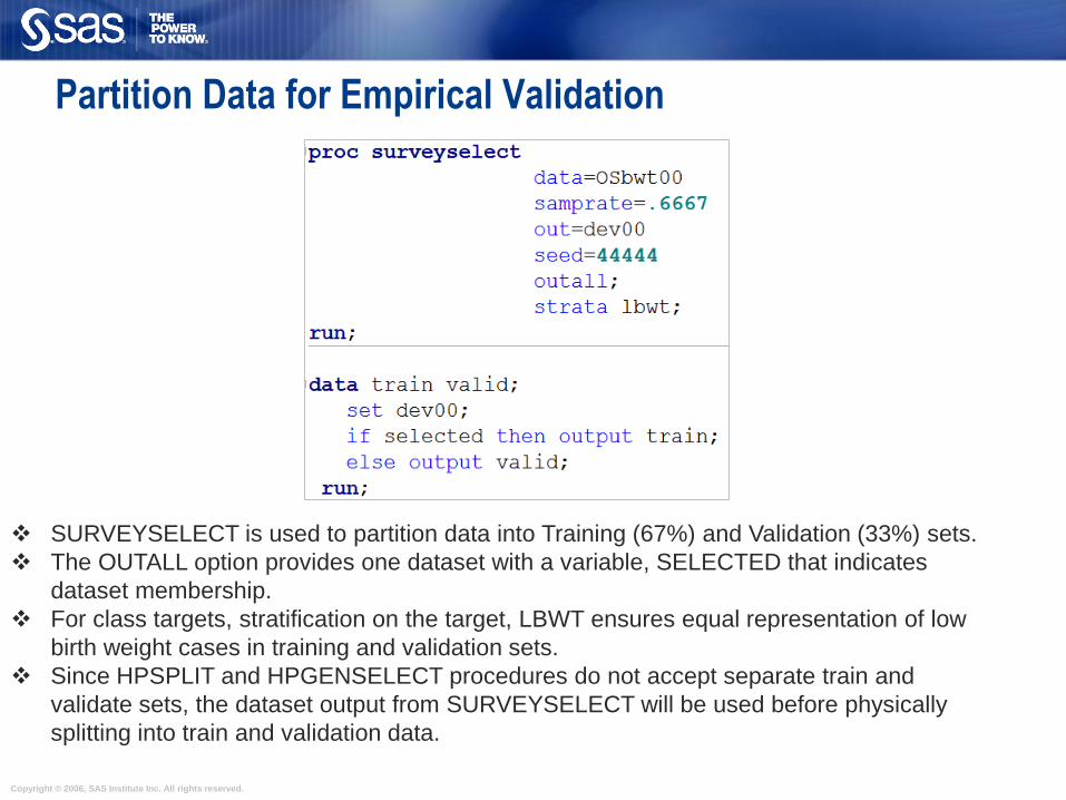
Partition Data for Empirical Validation
SURVEYSELECT is used to partition data into Training (67%) and Validation (33%) sets.
The OUTALL option provides one dataset with a variable, SELECTED that indicates
dataset membership.
For class targets, stratification on the target, LBWT ensures equal representation of low
birth weight cases in training and validation sets.
Since HPSPLIT and HPGENSELECT procedures do not accept separate train and
validate sets, the dataset output from SURVEYSELECT will be used before physically
splitting into train and validation data.
Copyright © 2006, SAS Institute Inc. All rights reserved.
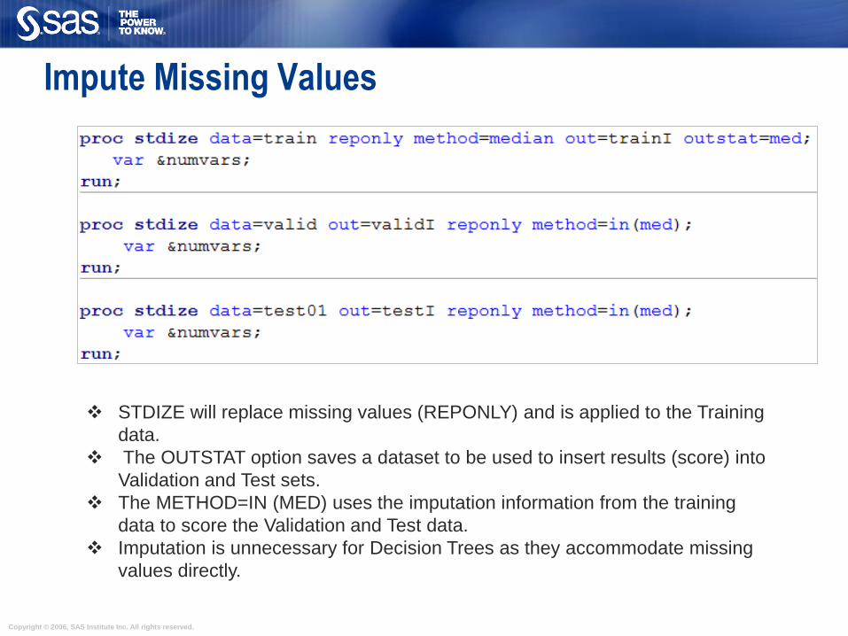
Impute Missing Values
STDIZE will replace missing values (REPONLY) and is applied to the Training
data.
The OUTSTAT option saves a dataset to be used to insert results (score) into
Validation and Test sets.
The METHOD=IN (MED) uses the imputation information from the training
data to score the Validation and Test data.
Imputation is unnecessary for Decision Trees as they accommodate missing
values directly.
Copyright © 2006, SAS Institute Inc. All rights reserved.
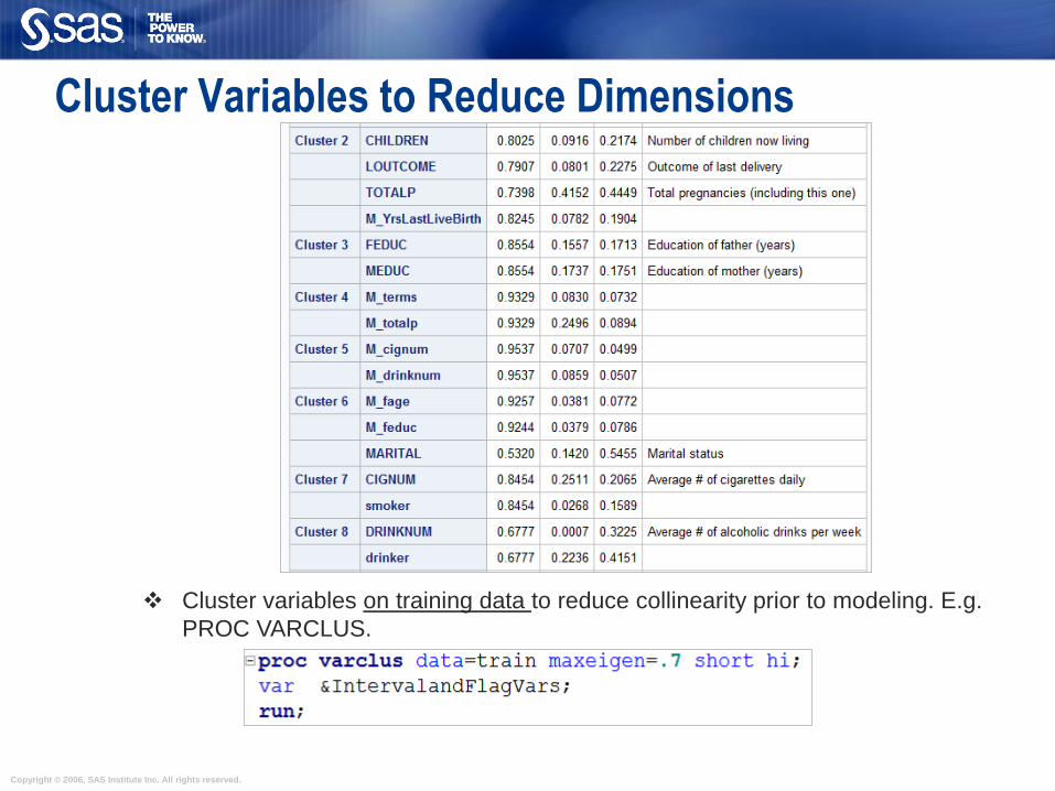
Cluster Variables to Reduce Dimensions
Cluster variables on training data to reduce collinearity prior to modeling. E.g.
PROC VARCLUS.

Copyright © 2006, SAS Institute Inc. All rights reserved.
Collapse Categorical Variables to Reduce Dimensions
Variables RACEMOM and RACEDAD contain 9 and 10 levels respectively.
Use a Decision Tree model to optimally collapse many possible combinations of
these attributes to a single 6-level variable using training data.
This step is unnecessary if you are using a decision tree as a predictive model.

Copyright © 2006, SAS Institute Inc. All rights reserved.
Binary Target Modeling

Copyright © 2006, SAS Institute Inc. All rights reserved.
New Modeling Routines in SAS/STAT: Decision Trees using HPSPLIT
In SAS 9.4 some of the high performance procedures used in Enterprise
Miner software for data mining are now available in SAS/STAT (now
called version 14.1).
Procedures support parallel processing and are designed to run in a
distributed computing environment (across multiple servers for high
speed computing).
Procedures are available to run on a single machine or server. They are
now shipped with SAS/STAT at no additional cost.
In this section we will feature HPSPLIT for decision trees using a binary
target and in a later section, HPGENSELECT for generalized linear
models and mixture distributions using a continuous target.
Copyright © 2006, SAS Institute Inc. All rights reserved.
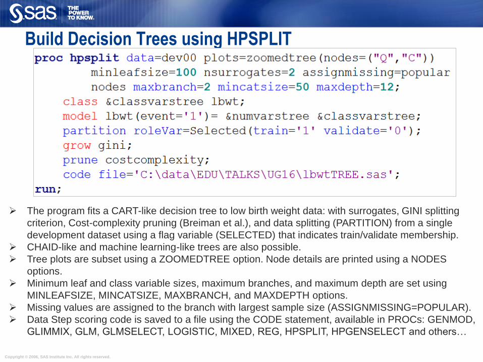
Build Decision Trees using HPSPLIT
The program fits a CART-like decision tree to low birth weight data: with surrogates, GINI splitting
criterion, Cost-complexity pruning (Breiman et al.), and data splitting (PARTITION) from a single
development dataset using a flag variable (SELECTED) that indicates train/validate membership.
CHAID-like and machine learning-like trees are also possible.
Tree plots are subset using a ZOOMEDTREE option. Node details are printed using a NODES
options.
Minimum leaf and class variable sizes, maximum branches, and maximum depth are set using
MINLEAFSIZE, MINCATSIZE, MAXBRANCH, and MAXDEPTH options.
Missing values are assigned to the branch with largest sample size (ASSIGNMISSING=POPULAR).
Data Step scoring code is saved to a file using the CODE statement, available in PROCs: GENMOD,
GLIMMIX, GLM, GLMSELECT, LOGISTIC, MIXED, REG, HPSPLIT, HPGENSELECT and others…
Copyright © 2006, SAS Institute Inc. All rights reserved.
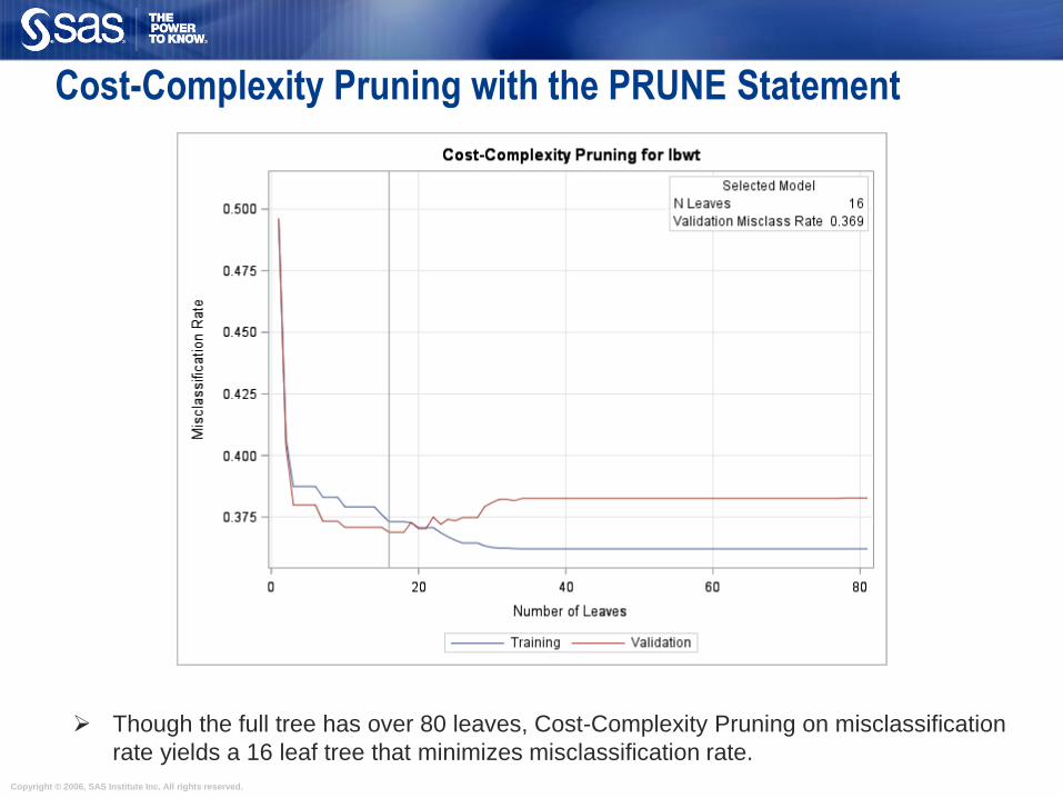
Cost-Complexity Pruning with the PRUNE Statement
Though the full tree has over 80 leaves, Cost-Complexity Pruning on misclassification
rate yields a 16 leaf tree that minimizes misclassification rate.

Copyright © 2006, SAS Institute Inc. All rights reserved.
The Final Tree
Nodes and leaves are
identified with numbers
and letters.
The width of the curves
are proportional to amount
of data passing through
each part of the tree.
Red indicates low bwt
classification while blue
indicates normal weight.

Copyright © 2006, SAS Institute Inc. All rights reserved.
Plot Tree Sections Using the ZOOMEDTREE option
Classifications using a cutoff of
0.5 are given at the top of each
node (e.g. Node T is classified
as low birth weight while Node
U is classified as normal
weight).
Samples sizes for
Train/Validate data, as well as
proportions of target 1 in each
are shown.
Red indicates low bwt
classification while blue
indicates normal weight.

Copyright © 2006, SAS Institute Inc. All rights reserved.
Display Leaf Rules using the NODES Option
… etc etc.
Rules details for all leaves are reported. Asterisk indicates selected target level.

Copyright © 2006, SAS Institute Inc. All rights reserved.
Explore Variable Importance
Race of mother and father as well as marital status and smoking behavior are the top
most important variables.

Copyright © 2006, SAS Institute Inc. All rights reserved.
Model Assessments
Training and Validation assessment measures and overlayed ROC curves are output.

Copyright © 2006, SAS Institute Inc. All rights reserved.
Score Data using HPSPLIT Scoring Code
Validation and Test data are scored using Decision Tree Scoring code.
Probabilities can be adjusted for oversampling (P_1ADJtree) if desired though this is not
required for ROC curve assessments.
Validation and Test scores from the tree model are match-merged back to the
corresponding imputed sets to be used for regression (not shown here).
Etc
Etc
Copyright © 2006, SAS Institute Inc. All rights reserved.
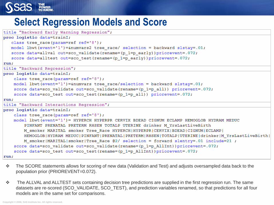
Select Regression Models and Score
The SCORE statements allows for scoring of new data (Validation and Test) and adjusts oversampled data back to the
population prior (PRIOREVENT=0.072).
The ALLVAL and ALLTEST sets containing decision tree predictions are supplied in the first regression run. The same
datasets are re-scored (SCO_VALIDATE, SCO_TEST), and prediction variables renamed, so that predictions for all four
models are in the same set for comparisons.

Copyright © 2006, SAS Institute Inc. All rights reserved.
Early Warning Regression Output, for example..
In general, predictive models fit to
larger datasets tend to have more
parameters than more theoretically
informed explanatory models in
health.
Odds ratios for previous premature
babies (PRETERM), renal disease
(RENAL), and chronic hypertension
(HYPERCH) and are particularly
large.
The collapsed version of mother and
father race from an initial decision
tree (TREE_RACE) appears in the
model.

Copyright © 2006, SAS Institute Inc. All rights reserved.
1 0
1
0
Predicted**
TP
FP
FN
TN AN
AP
PP PN n
Accuracy =
(TP+TN)/n
Sensitivity =
TP/AP
Specificity =
TN/AN
Lift =
(TP/PP)/π1
** - Where Predicted 1=(Pred Prob > Cutoff)
Model Assessments for Binary Targets

Copyright © 2006, SAS Institute Inc. All rights reserved.
TP
TN
FN
FP
TP
TN
FN
FP
TP
TN
FN
FP
TP
TN
FN
FP
TP
TN
FN
FP
TP
TN
FN
FP
Explore measures across a range of cutoffs
Lift Charts ROC Charts
Assessment Charts for Binary TargetsL
ift
Depth 1-SP
SE
Copyright © 2006, SAS Institute Inc. All rights reserved.
0.0
1.0
0.0 1.0
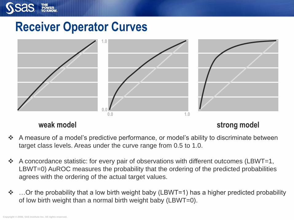
weak model strong model
Receiver Operator Curves
A measure of a model’s predictive performance, or model’s ability to discriminate between
target class levels. Areas under the curve range from 0.5 to 1.0.
A concordance statistic: for every pair of observations with different outcomes (LBWT=1,
LBWT=0) AuROC measures the probability that the ordering of the predicted probabilities
agrees with the ordering of the actual target values.
…Or the probability that a low birth weight baby (LBWT=1) has a higher predicted probability
of low birth weight than a normal birth weight baby (LBWT=0).

Copyright © 2006, SAS Institute Inc. All rights reserved.
Training
Validation
2000 2001
TEST
Predict the Future with Data Splitting
Models are fit to Training Data, compared and
selected on Validation and tested on a future Test
set.

Copyright © 2006, SAS Institute Inc. All rights reserved.
Assess Models using ROC Curves
The dataset with all four predictions (SCO_VALIDATE) is supplied to PROC LOGISTIC.
The ROCCONTRAST statements provides hypothesis tests for differences between ROC
curves, for model results specified in the three ROC statements.
To generate ROC contrasts, all terms used in the ROC statements must be placed on the
model statement. The NOFIT option suppresses the fitting of the specified model.
Because of the presence of the ROC and ROCCONTRAST statements, ROC plots are
generated when ODS GRAPHICS are enabled.
The identical process is repeated with the scored Test set, SCO_TEST. Can the model
predict the future?

Copyright © 2006, SAS Institute Inc. All rights reserved.
Compare ROC Curves on Validation Data

Copyright © 2006, SAS Institute Inc. All rights reserved.
Compare AuROC Curves on Validation Data

Copyright © 2006, SAS Institute Inc. All rights reserved.
Compare ROC Curves on Test Data
Copyright © 2006, SAS Institute Inc. All rights reserved.
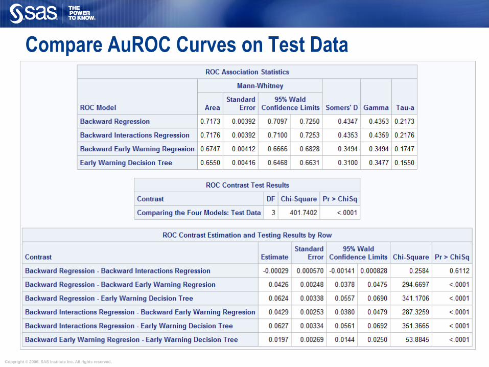
Compare AuROC Curves on Test Data
Copyright © 2006, SAS Institute Inc. All rights reserved.
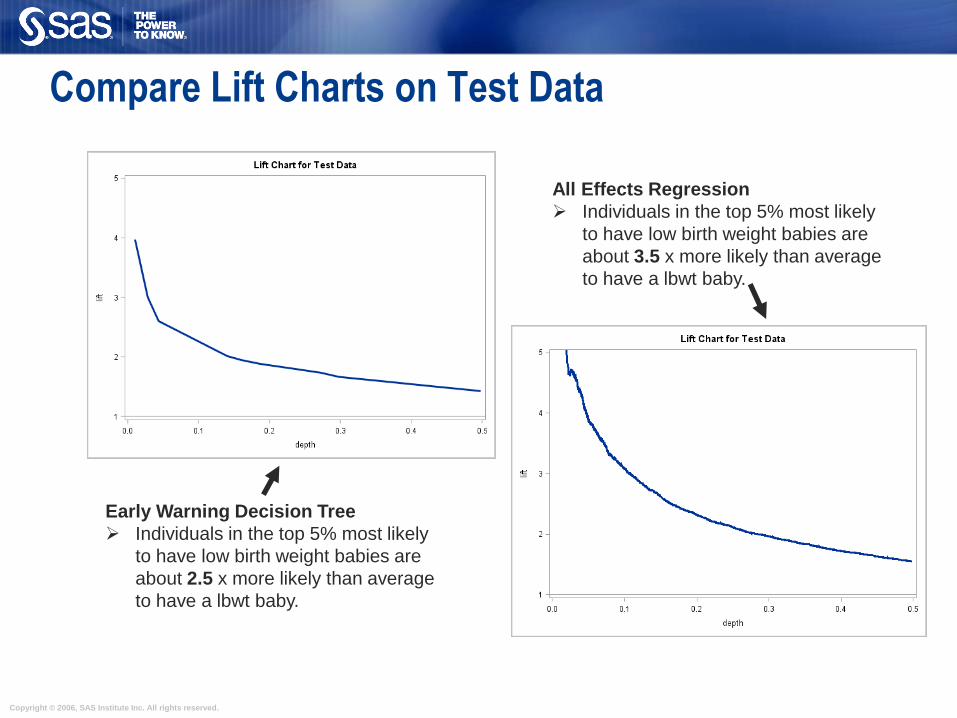
Compare Lift Charts on Test Data
Early Warning Decision Tree
Individuals in the top 5% most likely
to have low birth weight babies are
about 2.5 x more likely than average
to have a lbwt baby.
All Effects Regression
Individuals in the top 5% most likely
to have low birth weight babies are
about 3.5 x more likely than average
to have a lbwt baby.
Copyright © 2006, SAS Institute Inc. All rights reserved.
Continuous Target Modeling
Copyright © 2006, SAS Institute Inc. All rights reserved.
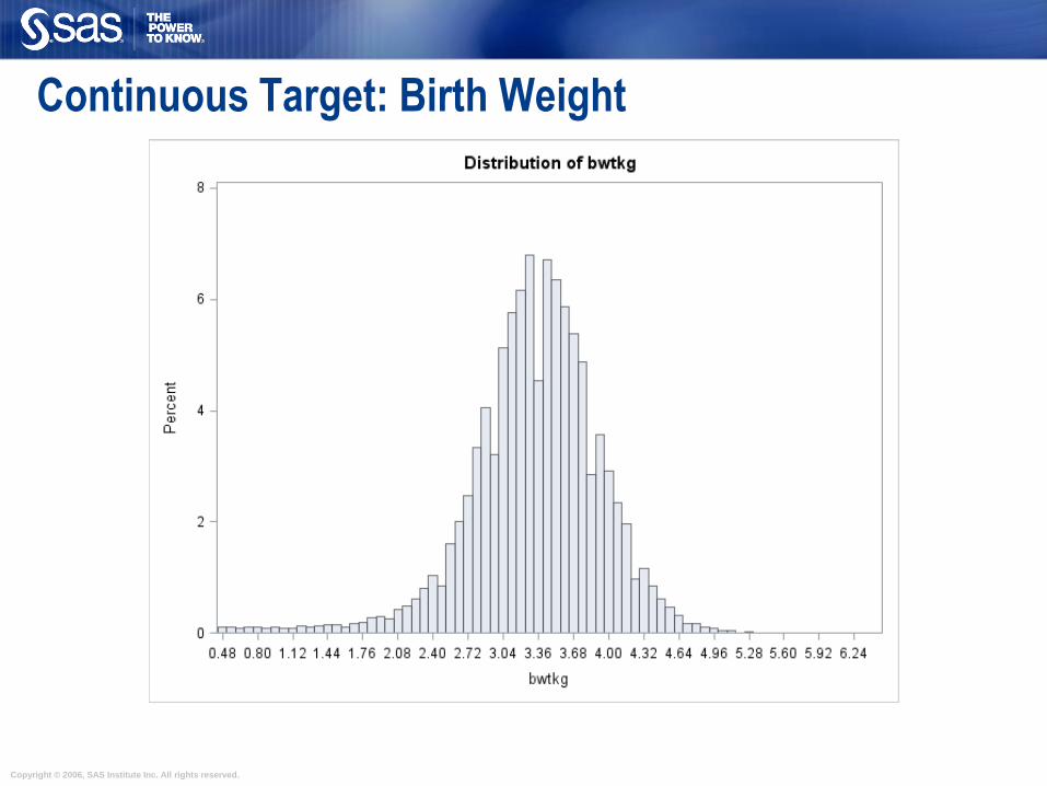
Continuous Target: Birth Weight

Copyright © 2006, SAS Institute Inc. All rights reserved.
Build Regression Models with GLMSELECT
GLMSELECT fits continuous target models (under GLM assumptions) and can process validation and test datasets, or perform cross validation for smaller datasets. It can also perform data partition using the PARTITION statement.
GLMSELECT supports a class statement similar to PROC GLM but is designed for predictive modeling.
Selection methods include Backward, Forward, Stepwise, LAR and LASSO.

Copyright © 2006, SAS Institute Inc. All rights reserved.
Least Angle Regression Standardize inputs and response. All coefficients are zero.
The predictor, X1 that is most correlated with the current residual (makes the least
angel with the residual) is determined and a step is taken in the direction of this
predictor (X1 is added to model). The length of this step (the coefficient
magnitude) is chosen so that some other predictor, X2 and the current predicted
response have the same correlation with the current residual (equiangular).
At this point, the predicted response moves in the direction that is equiangular
between (equally correlated with) these two predictors. Moving in this direction
ensures that these two predictors continue to have a common correlation with the
current residual.
The predicted response moves in this direction until a third predictor, X3 has the
same correlation with the current residual as the two predictors already in the
model. A new direction is determined that is equiangular between these three
predictors and the predicted response moves in this direction until a fourth
predictor joins the set having the same correlation with the current residual.
This process continues until all predictors are in the model.
Copyright © 2006, SAS Institute Inc. All rights reserved.
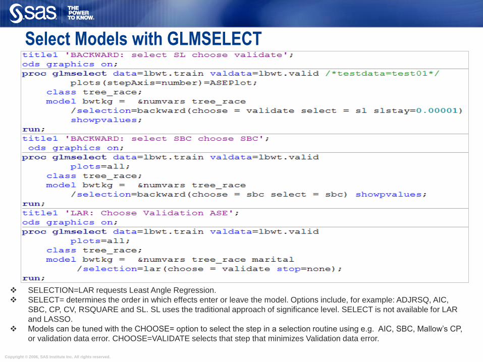
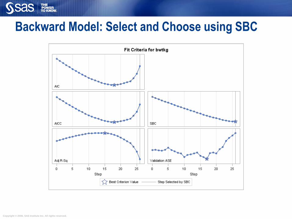
Select Models with GLMSELECT
SELECTION=LAR requests Least Angle Regression.
SELECT= determines the order in which effects enter or leave the model. Options include, for example: ADJRSQ, AIC,
SBC, CP, CV, RSQUARE and SL. SL uses the traditional approach of significance level. SELECT is not available for LAR
and LASSO.
Models can be tuned with the CHOOSE= option to select the step in a selection routine using e.g. AIC, SBC, Mallow’s CP,
or validation data error. CHOOSE=VALIDATE selects that step that minimizes Validation data error.

Copyright © 2006, SAS Institute Inc. All rights reserved.
Backward Model Tuning using Validation ASE
Copyright © 2006, SAS Institute Inc. All rights reserved.
Backward Model: Select and Choose using SBC

Copyright © 2006, SAS Institute Inc. All rights reserved.
LAR Model Tuning using Validation ASE

Copyright © 2006, SAS Institute Inc. All rights reserved.
Assess Final Model
GLMSELECT does not provide model diagnostics.
The model selected by GLMSELECT can be refit in PROC GLM.
PLOTS=DIAGNOSTICS requests diagnostic plots. With larger datasets the user
may have to increase the number of allowable plotting points using the
MAXPOINTS= option.
Copyright © 2006, SAS Institute Inc. All rights reserved.
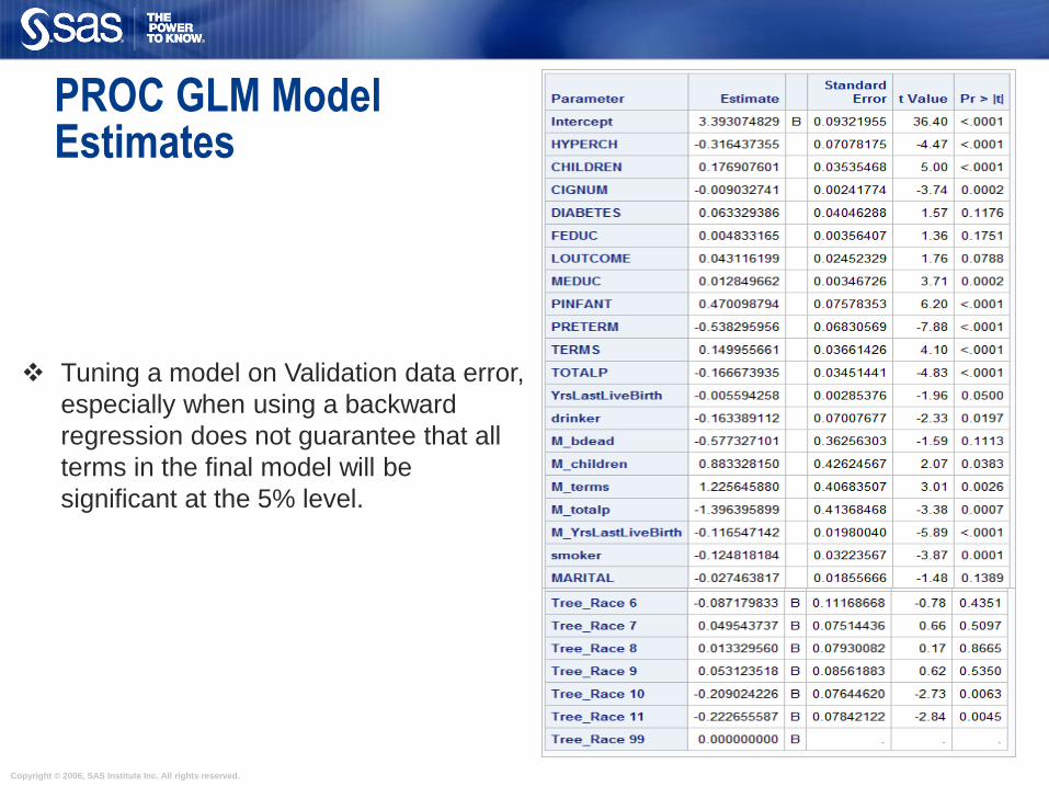
PROC GLM Model Estimates
Tuning a model on Validation data error,
especially when using a backward
regression does not guarantee that all
terms in the final model will be
significant at the 5% level.

Copyright © 2006, SAS Institute Inc. All rights reserved.
PROC GLM Statistical Graphics Diagnostics
ODS GRAPHICS ON and
PLOTS=DIANGOSTICS.

Copyright © 2006, SAS Institute Inc. All rights reserved.
Generalize Linear Predictive Modeling
Copyright © 2006, SAS Institute Inc. All rights reserved.
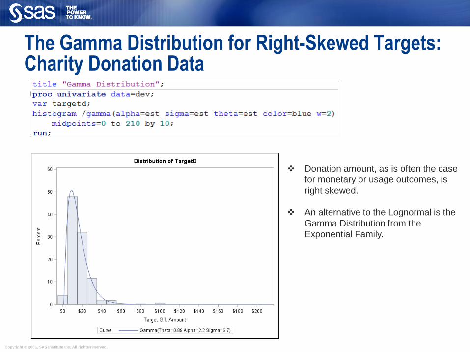
The Gamma Distribution for Right-Skewed Targets: Charity Donation Data
Donation amount, as is often the case
for monetary or usage outcomes, is
right skewed.
An alternative to the Lognormal is the
Gamma Distribution from the
Exponential Family.

Copyright © 2006, SAS Institute Inc. All rights reserved.
New Modeling Routines in SAS/STAT: Generalized Linear Models and Mixture Distributions using HPGENSELECT
Fits Generalized Linear Models by specifying a distribution and link
function to enable modeling of count data, rates, and non-normal
continuous outcomes.
Supports model selection routines Backward, Forward, Stepwise selection using significance level
LASSO selection
Choice of final model using significance level, AIC, SBC
Supports mixture distributions Zero Inflated Poisson
Zero Inflated Negative Binomial
Tweedie

Copyright © 2006, SAS Institute Inc. All rights reserved.
The Tweedie distribution has been used extensively in insurance data modeling as
it corresponds to the underlying loss generating process (e.g. total cost of claims).
This mixed type distribution results from the mixing of two underlying components
- the Poisson and Gamma distributions.
In the Zero-Inflated Poisson Model, the population is considered to consist of two
types of individuals. The first type gives Poisson distributed counts, which might
contain zeros. The second type always gives a zero count. The ZIP model fits,
simultaneously, two separate regression models. One is a logistic model that
models the probability of being eligible for a non-zero count. The other models the
size of that count.
Mixture Models with HPGENSELECT

Copyright © 2006, SAS Institute Inc. All rights reserved.
A single development dataset is supplied to the procedure. The PARTITION statement
requests a 67/33% split of this set.
A backward regression is run, eliminating terms based on statistical significance. The final
model in the backward sequence is chosen using the Schwartz Bayesian Criterion.
A Gamma distribution is fit using a log link (though inverse is the canonical link).
Fit a Gamma Regression to the Charity Donation Data

Copyright © 2006, SAS Institute Inc. All rights reserved.
The model at step 15 minimizes
SBC and is selected.
HPGENSELECT Output
Fit Statistics are
given for Training
and Validation data.
Estimates and
significance
tests are
provided.
Top Related