


Languages
Pages
Legal


1
Plant Productivity Dynamics and Private and Public R&D
Spillovers: Technological, Geographic and Relational
Proximity
René Belderbos
University of Leuven, UNU-MERIT, Maastricht University, and NISTEP
Kenta Ikeuchi*
NISTEP
Kyoji Fukao
Hitotsubashi University, NISTEP, and RIETI
Young Gak Kim
Senshu University and NISTEP
Hyeog Ug Kwon
Nihon University, NISTEP, and RIETI
This draft: September 11, 2013
Keywords: R&D, spillovers, plant productivity, distance JEL codes: D24, O32.
Acknowledgements
This paper is the result of a joint research project of the National Institute of Science and Technology
Policy (NISTEP) and the Research Institute for Economy, Trade and Industry (RIETI), Tokyo, Japan,
under the “Science for Science, Technology and Innovation Policy” program. The authors are grateful
to Masayuki Morikawa, Toshiyuki Matsuura, Chiara Criscuolo, Pierre Mohnen, Jacques Mairesse,
and participants at the NISTEP-RIETI Workshop on Intangible Investment, Innovation and
Productivity (Tokyo, January 2012), the 2012 CAED conference in Neurenberg (Germany), the
Workshop on Intangibles, Innovation Policy and Economic Growth at Gakushuin University
(December 2012, Tokyo) and the HIT-TDB-RIETI International Workshop on the Economics of
Inter-firm Networks (November 2012, Tokyo) for comments on earlier drafts. Rene Belderbos
gratefully acknowledges financial support from NISTEP and the Centre for Economic Institutions at
the Institute for Economic Research, Hitotsubashi University. * Corresponding author: Kenta Ikeuchi; Tel.: +81 (0)3 3581 2396; Email: [email protected]).

2
Plant Productivity Dynamics and Private and Public R&D Spillovers:
Technological, Geographic and Relational Proximity
ABSTRACT
We examine the effects of R&D spillovers on total factor productivity in a large panel of
Japanese manufacturing plants matched with R&D survey data (1987-2007). We
simultaneously examine the role of public (university and research institutions) and private
(firm) R&D spillovers, and examine the differential effects due to technological, geographic
and relational (buyer-supplier) proximity. Estimating dynamic long difference models
allowing for gradual convergence in TFP and geographic decay in spillover effects, we find
positive effects of technologically proximate private R&D stocks, which decay in distance
and become negligible at around 500 kilometres. Spillovers due to public R&D - corrected
for industrial relevance and technological proximity- are of a similar magnitude but are only
significant for plants operated by R&D conducting firms. Surprisingly, we do not find
evidence of geographic decay in the impact of public spillovers. In addition to knowledge
spillovers from technologically proximate R&D stocks, ‘pecuniary’ spillovers from buyer and
supplier R&D stocks exert positive effects on TFP growth that are relatively similar in
magnitude. Over time, declining R&D spillovers are responsible for a substantial part of the
decline in the rate of TFP growth. They appear to an important extent due to the exit of
proximate plants operated by R&D intensive firms. This occurred in particular in major
industrial agglomerations such as Tokyo, Osaka, and Kanagawa.

3
1. Introduction
It is well established in the literature that the productivity effects of R&D spillovers are
enhanced by technological proximity and geographic proximity (Jaffe et al, 1993; Adams and
Jaffe, 1996; Goto and Suzuki, 1989; Aldieri and Cincera, 2009; Lychagin et al., 2010; Bloom
et al., forthcoming; Orlando, 2004). Despite the increasing number of large-scale studies on
R&D spillovers, existing studies have a number of limitations in scope and methodology.
First, they typically relied on data on publicly listed firms, aggregating over the various
locations and technologies in which firms are active.1 Second, the focus has been on inter-
firm private spillovers while abstracting from the role of public research. A different research
stream focusing on the role of knowledge spillovers from public research conducted at
universities and research institutes has however suggested the importance of such spillovers,
with an explicit role of proximity (e.g. Jaffe, 1989; Adams, 1990; Anselin et al., 1997;
Furman et al., 2006). Third, R&D spillovers at the firm level have in most cases been
modelled as knowledge spillovers as a function of proximity between technology portfolios
of the firm, while the role of spillovers through supplier and customer linkages has only
received limited attention.2 A separate literature on the role of spillovers in the context of
foreign direct investments has strongly suggested that 'vertical' spillovers through buyer-
supplier relationships often is the key channel through with spillovers occur (e.g. Haskel et
al., 2007; Görg and Strobl, 2001; Javorcik, 2004; Kugler, 2006). While knowledge and
technology transfer in these relationships is often purposeful and embedded in intermediates,
their value tends not to be fully reflected in the price of such intermediates, leading to
‘pecuniary spillovers (Hall et al., 2012; Crespi et al, 2007). Compared with ‘horizontal’
spillovers in technological proximity within narrowly defined industries, the absence of
market rivalry provides greater incentives for productivity and growth enhancing knowledge
exchange and spillovers (e.g. Bloom et al., forthcoming). Since suppliers and clients may be
active in a variety of industries, these 'relational' spillovers are yet a different dimension of
heterogeneity in spillover pools.
This paper addresses these limitations in prior work. We contribute an analysis of the
various sources of R&D spillovers, which until now have not been examined simultaneously,
and examine these relationships at the plant level. We analyse the effects of technologically,
geographically, and relationally proximate private R&D stocks, as well as of technologically
1 Adams and Jaffe (1996) do analyse plant level productivity but focuses on the effects of internal R&D. 2 An exception is Crespi et al. (2007), who examine data from UK Community Innovation Surveys for direct
(self assessed) evidence of incoming knowledge flows at the firm level. They find, among others, that supplier
information positively affects TFP growth, but do not examine geographic or technological proximity.

4
and geographically proximate public R&D stocks on TFP in an unbalanced panel of close to
20000 Japanese manufacturing plants, 1987-2007. The plant level data from the Census of
Manufacturers are matched with information on R&D expenditures from the comprehensive
Survey of R&D Activities in Japan covering virtually all R&D spending firms (and public
institutions). The R&D survey data, which are decomposed by field or industry of application,
allow us to construct relevant R&D stocks weighted by technological proximity (e.g. Bloom
et al. forthcoming), while the information on plant locations allows us to explore the role of
geographic distance between firms and between firms and public research institutions in
much more detail than in previous studies. Relationally proximate R&D stocks are calculated
using input-output tables. Public R&D stocks are differentiated by science field, which can be
mapped into technologies and industries reflecting their varying relevance for firms. We
estimate long (five year) difference models of plant TFP growth to reduce the influence of
measurement errors and cyclical effects (e.g. Haskel et al, 2007; Branstetter, 2000). We allow
for gradual convergence in TFP by estimating dynamic TFP growth models (e.g. Klette,
1996; Lokshin et al., 2008), and we identify distance effects by estimating exponential decay
parameters (e.g. Lychagin et al., 2010). The simultaneous inclusion of multiple sources of
spillovers, the detail on location and field of R&D, the long panel, and the uniquely large set
of plants should allow more precise estimates of spillover effects and an assessment of their
relative importance over time. Our study contributes to the very limited literature on R&D
and spillovers at the plant level.
Our research is also motivated by the observation that Japan's total factor productivity
growth has been declining since the mid-1980s (e.g. Fukao and Kwon, 2011), while at the
same time R&D expenditures as a percentage of GDP have been steadily increasing to reach
3.8% in 2008, from 2.5% in 1980s. The discrepancy between the trends in R&D expenditures
and TFP suggests that the aggregate returns to R&D have been falling. One possible
explanation for this phenomenon may be a decline in R&D spillovers due to the relocation
abroad of sophisticated manufacturing plants of R&D intensive firms and the accompanied
changing patterns of R&D agglomeration, which may have reduced the size and effectiveness
of the relevant pool of R&D spillovers across firms.
The remainder of the paper is organized as follows. The next section describes the model,
the particularities of the data and the empirical strategy followed. Section 3 presents the
empirical results and section 4 concludes and discusses avenues for future research.

5
2. Model Setup and Data
We conduct a plant-level panel analysis of total factor productivity, in which we relate
plant-level TFP to firms’ own R&D stock, private R&D stocks (the private spillover pool),
public R&D stocks, and a set of plant-, firm- and industry-level controls. We assume that firm
level R&D stocks are available to all the firms’ plants and that R&D spillovers occur between
plants due to the R&D stock the plants have access to. This allows us to investigate the
geographic dimension of R&D spillover in detail, taking into account the population of R&D
conducting firms and the spatial and industry configuration of their plants.
We adopt the standard knowledge stock augmented production function framework (e.g.
Hall et al, 2012). We define the production function at the plant-level generally as:
𝑄𝑖𝑡 = 𝑓(𝐿𝑖𝑡, 𝐾𝑖𝑡, 𝑀𝑖𝑡)𝑔(𝑅𝑖𝑡−1, 𝑆𝑖𝑡−1, 𝑃𝑖𝑡−1, X𝑖𝑡)𝑈𝑖𝑡 (1)
Where:
𝑄𝑖𝑡: Gross output of the plant
𝐿𝑖𝑡, 𝐾𝑖𝑡, 𝑀𝑖𝑡: Inputs of plant 𝑖 in year 𝑡
𝑅𝑖𝑡−1: Firm-level R&D stock
𝑆𝑖𝑡−1: Private R&D stock
𝑃𝑖𝑡−1: Public R&D stock
X𝑖𝑡: a vector of other observable factors (control variables) affecting plant
productivity
𝑈𝑖𝑡: plant-year specific unobserved efficiency.
Total factor productivity (TFP) is defined as:
𝑇𝐹𝑃𝑖𝑡 ≡𝑄𝑖𝑡
𝑓(𝐿𝑖𝑡,𝐾𝑖𝑡,𝑀𝑖𝑡)= 𝑔(𝑅𝑖𝑡−1, 𝑆𝑖𝑡−1, 𝑃𝑖𝑡−1, X𝑖𝑡)𝑈𝑖𝑡 (2)
R&D stocks are assumed to influence production with a one-year lag to reflect that the
application of new knowledge and insights due to R&D takes time. If we adopt a log-linear
specification for 𝑔(𝑅𝑖𝑡−1, 𝑆𝑖𝑡−1, 𝑃𝑖𝑡−1) and allow 𝑈𝑖𝑡 = 𝑒𝜂𝑖+𝑢𝑖𝑡 , where 𝜂𝑖 is a plant specific
fixed effect and 𝑢𝑖𝑡 is a plant-year specific efficiency shock, we obtain:

6
ln 𝑇𝐹𝑃𝑖𝑡 = 𝛼𝑅 ln 𝑅𝑖𝑡−1 + 𝛼𝑆 ln 𝑆𝑖𝑡−1 + 𝛼𝑃 ln 𝑃𝑖𝑡−1 + γ′X𝑖𝑡 + 𝜂𝑖 + 𝑢𝑖𝑡 (3)
and if we difference the equation between two periods:
∆ln 𝑇𝐹𝑃𝑖𝑡 = 𝛼𝑅∆ ln 𝑅𝑖𝑡−1 + 𝛼𝑆∆ ln 𝑆𝑖𝑡−1 + 𝛼𝑃 ln∆ 𝑃𝑖𝑡−1 + γ′∆X𝑖𝑡 + ∆𝑢𝑖𝑡 (4)
where the plant-specific efficiency parameter drops out. We assume that the change in plant-
specific efficiency levels (∆𝑢𝑖𝑡) is a function of past productivity relative to the industry
mean, in order to allow for a gradual convergence in efficiency levels between firms (e.g.
Lokshin et al., 2008). Klette (1996) has shown that the empirically observed persistent
productivity differences between plants or firms require a model specification that allows for
gradual convergence.
⊿𝑢𝑖𝑡 = 𝑢𝑖𝑡 − 𝑢𝑖𝑡−1 = 𝜌ln𝑇𝐹𝑃𝑖𝑡∗ + 𝑒𝑖𝑡 (5)
where ln𝑇𝐹𝑃𝑖𝑡∗ is the level of TFP of plant 𝑖 relative to the industry mean in the previous
period. We expect 𝜌 to fall within the interval [-1,0]. If 𝜌 is zero there is no gradual
convergence between leading firms and lagging firms; if 𝜌 is –1 complete convergence
materializes in one period. We assume that the error term 𝑒𝑖𝑡 can be decomposed into four
components, year-specific effects 𝜆𝑡 , industry-year specific technological opportunity or
efficiency shocks 𝜇𝑠𝑡(with s denoting industry), regional shocks 𝜌𝑟 and measurement error
휀𝑖𝑡:
𝑒𝑖𝑡 = 𝜇𝑠𝑡 + 𝜆𝑡 + 𝜌𝑟 + 휀𝑖𝑡 (6)
Data sources and sample
We match plant level data from the Japanese Census of Manufacturers with information
on R&D expenditures from the yearly (comprehensive) Survey of R&D Activities in Japan,
1987-2007. The census has a comprehensive coverage of manufacturing plants with more
than 4 employees. From 2001 onwards, information on plant level fixed capital investment
has not been surveyed for plants with less than 30 employees, with the exception of the
benchmark surveys organized every 5 years. The number of plants for which panel data on
TFP can be calculated is roughly 40,000 yearly.

7
The Survey of R&D activities in Japan is a comprehensive and mandatory survey of
R&D performing firms and public research institutes and universities in Japan. It contains
information on R&D expenditures, differentiated by field, for roughly 9,000 firms yearly and
has a response rate greater than 90 percent. Large firms (with more than 1 billion Yen of
capital) are always included in the survey; smaller firms are included in higher sampling rates
if they are identified as R&D conducting firms in their last survey. The information on R&D
by field (30 fields are distinguished) is easily mapped into industries, and allows us to
distinguish R&D expenditures relevant to 21 manufacturing industries. The response rate by
research institutes and universities is close to 100 percent.
The matching between the surveys posed a number of challenges. Firm names are only
recorded in the R&D survey from 2001 onwards and parent firm names are only provided on
the plant records in the census from 1994 onwards. Firm identifiers in the R&D survey are
not compatible between the years before and after 2001 because the identifiers for all firms
were revised in 2001; only the R&D survey in 2001 includes both the old and new versions
of firm identifiers. Because of the absence of common firm identifiers in the surveys,
matching had to be done semi-manually (by firm name, address and capitalization). From
2001 onwards, we could match more than 97,5 percent of reported R&D expenditures to
firms and plants included in the census (Figure 1). The situation is more complicated for the
years 1983-2000, for which we could only match R&D to plants 1) that could be linked to the
parent firm in 1994 or one of the later years, and 2) that belong to firms identified in the R&D
survey of 2001. This caused the coverage rate to decline from 98 percent in 2001 to 92,5
percent in 2000, declining progressively further to 73 percent in 1983.
Insert Figure 1
The matching issues cause several problems. First, there is a difficulty ascertaining
whether a plant belongs to a parent firm conducting R&D or not. Here we excluded all
unmatched firms from our sample to avoid measurement error in R&D stocks at the firm
level. Second, for some firms R&D series are incomplete. We proceeded to calculate R&D
stocks on the basis of the information available only if there was sufficient information to
derive an R&D growth rate for a specific period. Firms that are included in the R&D survey
multiple times reporting absence of R&D activities are included in the sample with zero R&D
stock. Third, we require reliable estimates of private R&D spillover pools. Here we obtained
estimates that are as accurate as possible by 1) using the weights provided in the R&D survey
8
to correct for non-response and arrive at an estimate of total R&D expenditures in Japan; 2)
allocating the R&D (stocks) to locations and fields/industries for R&D conducting firms that
could not be matched to the manufacturing census (and hence for which no geographic
information on plants is available) on the basis of the location of the firm, rather on the basis
of the location of plants. The second correction may be a reasonable approximation as most
of the unmatched firms are smaller enterprises with plants and administrative unit located in
the same city or prefecture.
Using the above matching rules, we obtain an unbalanced panel of over 19000 plants,
observed for a maximum of 20 years and a minimum of 5 years, during 1987-2007. The five
year minimum observation period is due to the fact that we will estimate (five-year) long
difference models. About 62 percent of the plants are owned by parent firms for which we
could confirm the absence of formal R&D. Zero R&D cases are not compatible with the
specification in natural logarithms in (4) but provide important variation in the sample. We
deal with this in two ways. We add the value 1 to the R&D stock before taking the logarithm,
such that we treat the continuous absence of R&D as zero growth. Second, we include a
dummy for continuous engagement in, or absence of, R&D.
Table 1 shows the distribution of plants over industries and compares this with the
distribution of the population of Japanese manufacturing plants over industries. Plants in
technology intensive industries such as drugs & medicine and chemicals are overrepresented
in our sample, but the difference with the distribution of all plants over industries is not
generally pronounced. The 19389 unique plants are operated by 13188 firms, implying that
on average there are 1.5 plant observations per firm in the sample. Parent firm R&D stocks
are highest in the home electronics and information and telecommunication sectors, and
lowest in pulp & paper and printing.
Insert Table 1
We note that creating a sample of plants for which parent firms’ R&D stocks can be
calculated leads to various sample selection issues, with a natural oversampling of R&D
conducting firms (although the majority of plants in our sample have no access to internal
R&D), larger plants (post-2001), surviving plants (1987-1994), and surviving firms (1987-
2001). Our aim is to conduct several sensitivity analyses to examine potential selection bias,
such as estimating models for the entire population of plants for which TFP can be calculated,
while including a dummy for unmatched R&D; estimating models only for the post-2000
9
period; and estimating models in different five year periods such that the share of small plants
is increased.
Variables and Measurement
We utilize plant level TFP data from the Japan Industrial Productivity Database (JIP)
2010 (Fukao et al., 2007). TFP is measured using the index number method, following Good
et al (1997):
ln𝑇𝐹𝑃𝑓𝑠𝑖𝑡 = (ln 𝑄𝑓𝑠𝑖𝑡 − ln 𝑄̅̅ ̅̅ ̅𝑠𝑡) − ∑
1
2(𝑠𝑓𝑠𝑖𝑡
𝑋 + �̅�𝑠𝑡𝑋 )(ln 𝑋𝑓𝑠𝑖𝑡 − ln 𝑋̅̅ ̅̅ ̅
𝑠𝑡)
𝑋=𝐿,𝐶,𝑀
+ ∑(ln 𝑄̅̅ ̅̅ ̅𝑗 − ln 𝑄̅̅ ̅̅ ̅
𝑗−1)
𝑡
𝑗=1
− ∑ ∑1
2(�̅�𝑓𝑠𝑖𝑗
𝑋 + �̅�𝑠𝑗−1𝑋 )(ln 𝑋̅̅ ̅̅ ̅
𝑠 − ln 𝑋̅̅ ̅̅ ̅𝑠−1)
𝑋=𝐿,𝐶,𝑀
𝑡
𝑗=1
(1)(7)
where Qfsi,t is the gross output of plant i of firm f in industry s in year t, sX,fsi,t is the cost share
of input X, and Xfsi,t is the amount inputs of the plant. Three inputs, labour (L), capital (C),
and intermediate input (M), are taken into account. Variables with upper bars denote the
arithmetic mean of each variable over all plants in that industry s in year t. The JIP database
provides index linked TFP estimates distinguishing 58 industries. The TFP indices express
the plants’ TFP as an index of the TFP level of a hypothetical representative plant in the
industry (with an index of 1). One of the main advantages of the index number method is that
it allows for heterogeneity in the production technology of individual firms, while other
methods controlling for the endogeneity of inputs (e.g. Olley and Pakes, 1996; Levinsohn and
Petrin, 2003) assume an identical production technology among firms within an industry (Van
Biesebroek, 2007; Aw et al. 2001).
Figure 2 shows the 5-year moving average of the gross output weighted average TFP
growth rate for the sample. The figure confirms that the rate of TFP growth has been
decreasing over time, while there is a modest recovery in growth rates in after 1999. The
pattern of TFP growth in the sample closely follows the pattern of TFP growth in the
population of Japanese plants.
Insert Figure 2
R&D stocks by industry and location
R&D stocks measured at the parent firm level can be separated by industry/field of
application to arrive at R&D stocks of the firm per industry. We utilize a question in the R&D
10
survey asking firms to allocate R&D expenditures by field, which easily maps into 25
industries. R&D stock of firm 𝑓 in industry/field s is defined by:
𝐾𝑓𝑠𝑡 = 𝐼𝑓𝑠𝑡 + (1 − 𝛿𝑠)𝐾𝑓𝑠𝑡−1 (8)
where 𝐼𝑓𝑠𝑡 is R&D investment of firm 𝑓 for activities in industry 𝑠 in year 𝑡 and 𝛿 is a
depreciation rate of the R&D stock. We use industry-specific depreciation rates to reflect
differences in the speed of obsolescence and technology life cycles. Industry specific
depreciation rates are based on Japanese official surveys of “life-span” of technology
conducted in 1986 and 2009 among R&D conducting firms 3 and vary between 8 (food
industry) and 25 percent (precision instruments). To calculate initial R&D stocks (Hall and
Oriani, 2006), we similarly use industry-specific growth rates, which we calculate from the
R&D survey as average R&D growth rates per field in the 1980s. R&D investments are
deflated using a deflator for private R&D from the JIP database (calculated from the price
indices of the input factors for R&D expenditures for each industry); the deflator for public
R&D is obtained from the White Paper on Science and Technology.
Matching the field of firms’ R&D with the industry of the firms’ plants, we can
calculate R&D stocks across industries and space, where we assume that the R&D stock is
available to each same-industry plant of the firm. We map R&D stocks in geographic space
by using the information on the location of the plant, where we distinguish more than 1800
cities, wards, towns, and villages.
Plant R&D stocks
We calculate plant R&D stocks as the R&D stock of the parent and assume that all parent
R&D provides relevant productivity improving inputs to the plants. Given that R&D at the
firm level is often organized to benefit from scope economies (e.g. Henderson and Cockburn,
1996; Argyeres and Silverman, 2004) and involves active knowledge transfer to business
units and plants, this may be a suitable assumption.4
3 “White paper on Science and Technology” (1986, Science and Technology Agency) and “Survey on Research
Activities of Private Corporations” (2009, National Institute of Science and Technology Policy). 4 We also calculated a technological proximity weighted parent R&D stock, applying the weighting scheme for
industries/fields outside the industry of the plant based on the technological proximity matrix used for R&D
spillovers, but obtained weaker effects. As the co-occurrence of different technologies in the R&D portfolios of
firms is often taken as an indicator of the potential for scope economies (Bloom et al. forthcoming; Breschi et al.
2003) this is perhaps not surprising.

11
Private R&D stocks (spillover pools)
Private R&D stocks (spillover pools) are derived from the calculated parent firms’ R&D
stocks by field and technological and relational proximities between plants, while we allow
for geographic decay in the effectiveness of spillovers. Technologically proximate R&D
stocks are calculated based on the technological proximity between the R&D field of the
plant’s industry and the R&D fields of other plants. We define the technologically relevant
private R&D stock (spillover pool) as the sum total of other firms’ R&D assigned to their
plants on the basis of the industry, weighted by the technological relatedness with the field of
the plant:
𝑆𝑖𝑓𝑠𝑡𝑡𝑒𝑐ℎ = ∑ ∑ 𝐾𝑓′𝑠′𝑡𝑇𝑠𝑠′𝑒
𝜏𝑑𝑖𝑓′𝑠′𝑡
𝑠′𝑓′≠𝑓 (10)
where:
𝑑𝑖𝑓′𝑠′𝑡: Minimum geographic distance between plant 𝑖 and the plant of firm 𝑓′ in the
field 𝑠′ in year 𝑡;
𝑇𝑠𝑠′: the technological proximity weight;
𝑒𝜏𝒅
𝑖𝑓′𝑠′𝑡: Weight for geographic proximity of plant 𝑖 to R&D stock firm 𝑓′ for field
𝑠′;
𝜏: a decay parameter, with 𝜏 < 0.
If firms operate multiple plants, the R&D stock is only counted once using the plant with
the minimum distance to the focal plant, which avoids double counting of R&D. 5 We model
an exponential decay function in the effectiveness of spillovers with parameter 𝜏 to be
estimated, in line with recent studies (e.g. Lychagin et al. 2010). Distance d is the distance
between a pair of locations and is measured as the geo-distance between the centre of cities,
wards, towns, and villages. In order to correct for differences in the geographic areas covered
by the regions, distance is the radius of the region if plants are located in the same region.
Our technological relatedness measure is derived from patent data and based on Leten et
al. (2007). The relatedness between technologies will be reflected in the intensity with which
technologies in a field build on prior art in a different field. Patent citation data are available
5 This would follow from the notion of redundancy in the type of R&D spillovers. On other hand, one may
argue that having multiple plants in the vicinity increases the likelihood of knowledge spillovers.

12
at the 4-digit IPC level. The IPC codes can subsequently be mapped onto industries using the
industry-technology concordance table developed by Schmoch et al. (2003) in which each
technology field is uniquely linked to its corresponding NACE two-digit industry. Appendix
A shows the resulting technological relatedness coefficients (weights) between industries
used in our analyses, with weights for the own industry normalized at 1.
We measure relationally proximate R&D stocks by the R&D stocks of supplier and
customer industries, identifying the importance of supplier and customer transactions from
Input-Output tables for 58 JIP industries. The calculation of R&D stocks follows (10) but
with 𝑇𝑠𝑠′ substituted by supplier industry proximity weights 𝑆𝑈𝑃𝑠𝑠′ and customer proximity
weights 𝐶𝑈𝑆𝑠𝑠′ , with:
𝑆𝑈𝑃𝑠𝑠′𝑡 =𝑄
𝑠′𝑠𝑡
∑ 𝑄𝑗𝑠𝑡𝑗 (12)
𝐶𝑈𝑆𝑠𝑠′𝑡 =𝑄
𝑠𝑠′𝑡
𝐸𝑋𝑠𝑡+𝑄𝑠𝑡 (13)
Where 𝑄𝑠′𝑠𝑡 denotes domestic sales of industry 𝑠′ to industry 𝑠 and 𝐸𝑋𝑠𝑡 denotes exports of
industry𝑠. In equation (12), (𝑄𝑠′𝑠𝑡 ∑ 𝑄𝑗𝑠𝑡𝑗⁄ ) is the share of industry 𝑠′sales to industry s in
the sum of sales by all industries j to industry s (input share)6. Weights for customer R&D
stocks are the shares of sales by industry s to industry 𝑠′ in total sales (export plus total
domestic sale) industry s. We use the 5-yearly input output tables with interpolation for
intermediate years, such that weights are varying by year. Appendix B and C shows the input
and output share of industries used in the analysis.
Public R&D stocks
Public R&D spillover pools derived from the R&D surveys have few measurement
issues, as response rates are virtually 100 percent. We differentiate public R&D by location
based on the region (city, ward, town, village) of the research institute or university, and by
industry/R&D field utilizing information on science fields with varying relevance for specific
industries. We define the R&D stock of public research institution ℎ in science field 𝑚 as:
6 Domestic sales in the Input-Output table include domestic sales of imported goods, 𝑄
𝑠′𝑠𝑡+ 𝐼
𝑠′𝑠𝑡, while
these sales of imported goods are not differentiated by industry of destination. We estimate sales due to
domestic output by multiplying total sales in the IO table by the ratio of domestic output 𝑄𝑠𝑡 to imports:
𝑄𝑠′𝑠𝑡
= (𝑄𝑠′𝑠𝑡
+ 𝐼𝑠′𝑠𝑡
) ∗ 𝑄𝑠𝑡/(𝑄𝑠𝑡 + 𝐼𝑠𝑡).

13
𝐴ℎ𝑚𝑡 = 𝐸ℎ𝑚𝑡 + (1 − 𝛿𝐴)𝐴ℎ𝑚𝑡−1 (14)
where 𝐸ℎ𝑚𝑡 is research expenditure of public research institution ℎ in science field 𝑚 in year
𝑡 and 𝛿𝐴 is a depreciation rate of public R&D stock, which we set at 15 percent per year.
Although the surveys do not include research expenditures by science field, they do contain
information on the number of researchers by science field for each institution for each year.
We estimate the public R&D expenditure 𝐸ℎ𝑚𝑡 by mutliplying total R&D expenditures with
the share of the number of scientists in the field in the total number of scientists for each
institution and year.
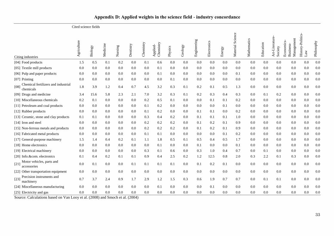
Second, we estimate a ‘relevant’ public R&D stock per industry/R&D field using weights
derived from a concordance matrix between science fields and industries. The weights are
based on a study by Van Looy et al. (2004) examining citation frequencies to Web of Science
publications in each of the scientific disciplines as observed on patent documents classified in
different technology fields. The concordance attaches to each scientific discipline
probabilities that it is of relevance to each technology field (4-digit IPC fields). We can easily
map the academic fields distinguished in the R&D survey to the scientific disciplines
distinguished in the Web of Science. We can subsequently apply the concordance matrix
between IPC classes and industries due to Schmoch et al. (2004) to arrive at public R&D
stocks per industry. Appendix D shows the compound weights used to relate R&D stocks per
science field to industries.
Using the above procedure, the technologically and geographically proximate public R&D
stock is defined as:
𝑃𝑖𝑡𝑠 = ∑ ∑ 𝐴ℎ𝑚𝑡�̃�𝑠𝑚𝑒𝜃�̃�𝑖ℎ𝑚ℎ (14)
Where:
𝐴ℎ𝑚𝑡: R&D stock of public institutes in location ℎ for academic field 𝑚 in year 𝑡;
�̃�𝑠𝑚: The compound proximity weights between industry/R&D field 𝑠 and science
field 𝑚;
�̃�𝑖ℎ: geographic distance between plant 𝑖 and location ℎ;
𝜃: the geographic decay parameter, 𝜃 < 0.
Figure 3 shows the 5-year moving average growth rates in the levels of public and
private R&D stocks. Both R&D stocks show a declining trend, as the increase in overall

14
R&D investments (Figure 1) has been generally insufficient to compensate R&D the effects
of depreciation.
Insert Figure 3
Control variables
The vector of time varying plant-specific characteristics X𝑖𝑡 includes plant size (number of
employees) and a dummy variable indicating whether the plant is active in multiple industries
(at the 4 digit level).7 In addition, we control for parent firm size (number of employees) and
the number of plants of the parent firm. On the one hand, increases in the number of a firm’s
plants may correlate with unmeasured firm-specific advantages. On the other hand a larger
numbers of plants drawing on the same R&D pool may lead to reduced effective knowledge
transfer (Adams and Jaffe, 1996). We include a set of year dummies 𝜆𝑡 and region
(prefecture) dummies 𝜌𝑟. We model 𝜇𝑠𝑡 as a set of industry dummies 𝜇𝑠 in addition to the
average TFP growth rate for all plants in the industry, ln 𝑡𝑓�̃�𝑠𝑡 , which controls for industry-
specific shock over time affecting TFP growth.
Specification
We estimate equation (4) in its long difference form. Long difference models, while
sacrificing degrees of freedom, is a conservative estimation method to reduce the influence of
measurement error and cyclical effects (e.g. Haskel et al, 2007; Branstetter, 2000). To strike a
balance between degrees of freedom and reduction in measurement error, we take 5-year
differences starting from 1987, which leaves a maximum of exactly 4 non-overlapping long
difference observations (for plants observed over the entire period): 1987-1992, 1993-1997,
1998-2002 and 2003-2007. To facilitate interpretation, we calculate the annual average
growth rate based on this 5-year difference, such that the dependent variable corresponds to a
yearly growth rate. Since the geographic decay specification introduces nonlinearity in the
TFP equation, we estimate equation (4) with nonlinear least squares. Error terms are cluster-
robust at the plant level.
Table 2 shows descriptive statistics of the variables and Table 3 contains the correlation
matrix. The correlations between the relationally proximate R&D stocks (buyers and
suppliers) and the technologically proximate R&D stock are rather high at 0.66-0.78. This is
mainly stemming from own industry R&D stock correlation, and correlations between stocks
7 Note that age effects are of no interest in differenced models, since the difference in age would be identical for
all plants.

15
limited to other industries range between -0.04 and 0.12. Hence, the different measures of
proximity do suggest rather different weightings for R&D stocks and the resulting spillovers
potential.
Insert Tables 2 and 3
3. Empirical results
Table 4 reports the estimation results. Model 1 includes the technologically proximate
R&D stock, the parent firm R&D stock, and the public R&D stock. The coefficient on parent
R&D suggests an elasticity of TFP with respect to R&D of 0.033 percent, which is within,
but at the lower end, of the range estimated in Adams and Jaffe (1996) for plant level R&D
effects.8 The elasticity of the private R&D stock is higher – a common finding in R&D
spillover studies- at 0.05, while spillover effects decay in distance, as the significant distance
parameter suggests. The coefficient on public R&D is positive but insignificant.
Insert Table 4
The estimates on the past TFP level suggest that plants that are 1 percent more
productive than the average TFP level in the industry, have a 0.08 percent point smaller TFP
growth rate, indicating that there is a modest gradual convergence in productivity. TFP
growth of the plants is strongly influenced by opportunities and shocks captured by the
average TFP growth in the industry, with an estimated elasticity of 0.89. None of the plant
and firm control variables has a significant effect on productivity growth. In model 2 we add
the dummy variable indicating continuous positive R&D. Both the dummy variable
indicating positive R&D and the R&D stock are significant. The dummy variable suggests
that R&D performing firms generate on average 0.5 percent points higher TFP growth. At the
same time, the coefficient of the parent R&D stock declines to about 0.01.
The absence of an estimated impact of public R&D may be related to a lack of absorptive
capacity of firms to screen, understand, and utilize the fruits of relevant scientific research
(Cohen and Levinthal, 1990). Prior studies have suggested that firms need to invest in
internal R&D in order to benefit from academic research (e.g. Cassiman and Veugelers,
2006; Anselin et al., 1997; Belderbos et al. 2009). In model 3, we separate the effect of public
8 We note that their specification was cross sectional, and one may expect smaller effects in a differenced model.

16
R&D into an effect for firms with zero R&D and an effect for firms with positive R&D. The
results confirm that R&D investment is a necessary condition for public R&D spillovers to
occur. Public R&D spillovers are significant with a coefficient (0.055) exceeding the
coefficient of private R&D spillovers, while for firms without R&D, public R&D spillovers
have no significant impact. Surprisingly, though, the estimates do not suggest a significant
geographic decay effect of public R&D spillovers.
In models 4-6 the relationally proximate R&D stock variables are added: supplier
spillovers in model 4, customer spillovers in model 5, and both spillovers in model 6. The
relationally proximate R&D stock due to supplier linkages has a significant effect on TFP
growth with elasticity slightly smaller than technologically proximate R&D, at 0.04; this
reduces to 0.034 in model 6 with all private R&D stocks included. The significant elasticity
of customer R&D stocks in model 5 is slightly smaller at 0.036 and is reduced to 0.027 in
model 6. Meanwhile, the coefficient on technologically proximate R&D stocks is only
marginally affected. The main conclusion from model 6 is that relationally proximate R&D
stocks generate ‘pecuniary’ R&D spillovers on top of the knowledge spillovers due to
technologically proximate R&D. As with public spillovers, however, we cannot identify a
geographic decay in this effect. For technologically proximate R&D spillovers, the decay
function on the basis of model 6 is depicted in Figure 6. Spillover effects decline and become
negligible at about 500-600 kilometers.
Insert Figure 4
Sensitivity analysis
We further explored the role of distance for public spillovers and the assumption that
(private) R&D spillovers as a function of distance play out at the plant level. In an alternative
specification, we examine distance between the firms’ R&D laboratories and between R&D
laboratories and public R&D. In particular for public spillovers, linkages may occur at the
laboratory level and not necessarily at the plant level, while the R&D laboratories may not
necessarily be located close to the firms’ plants. We derive the location of R&D laboratories
from published directories of R&D establishments in Japan. For R&D performing firms
lacking laboratory location information, we assign R&D to the location of headquarters – the
safest option for these -mostly smaller- firms (e.g. Adams and Jaffe, 1996; Orlando, 2004).
Our –still preliminary- results did not show geographic decay effects in this specification
either.

17
We aim to conduct a number of additional sensitivity analyses. First, we estimate
productivity models for the entire population of Japanese manufacturing plants to examine
the robustness of our estimates. Here we treat the unmatched plants as zero R&D plants while
including a separate dummy variable representing that the plants lack R&D information.
Second we estimate the model without smaller plants, to generate more consistency in the
sample across years. Third, we explore the sensitivity of the results to changes in the length
of the long difference, by examining models based on 10 year differences. Fourth we
examine the importance of taking into account technological proximity and relevance for
private and public spillovers by estimating models omitting such weights from the calculation
of R&D stocks.
Decomposition analysis
Given the time dimension in our data and the changes over time in R&D investments and
agglomeration, we can decompose long term TFP growth effects into several factors: plant
internal R&D effects, private R&D spillovers effects, and public R&D spillovers effects.
Results (details of which are to be included in the future version of this paper) indicate that
declining R&D spillovers, in particular private R&D spillovers, play an important role in the
decline in TFP growth in the sample firms over the years. We can further decompose the
changing private R&D spillovers into effects due to exit of plants, entry of plants, and
surviving plants. This exercise shows that in particular the exit of plants operated by R&D
intensive parent firms has an important role to play in spillovers declines. Most of these exits
appear to have taken place in the major industrial agglomerations in Japan around Tokyo,
Osaka, and Aichi (home of an automobile cluster led by Toyota).
4. Conclusions
This paper examines the effects of R&D spillovers on total factor productivity in a large
panel of Japanese manufacturing plants matched with R&D survey data. We simultaneously
analyse the role of public (university and other institutes) and private R&D spillovers
controlling for parent firm R&D, while examining effects due to relational (supplier-
customer) proximity as well as technological and geographic proximity. Our analysis
confirms the importance of positive spillovers effects from R&D by firms with plants in the
technologically related industries. The latter spillover effects are attenuated by distance and
our estimates suggest that most spillover effects disappear beyond 500 kilometres. We also
find positive effects of public R&D spillovers, but these effects only occur for plants with

18
access to internal R&D. Surprisingly, we do not find evidence that public R&D spillover
effects are attenuated by distance. In addition to knowledge spillovers from technologically
proximate plants, we find evidence that ‘relational proximity’ due to buyer and supplier
linkages generates additional ‘pecuniary’ R&D spillovers of relatively similar magnitude as
the knowledge spillovers. We could not identify the role of geographic distance in these buyer
and supplier spillovers.
Decomposition analysis shows that the contribution of private R&D spillovers to TFP
growth has declined since the late 1990s. Next to the decline in growth in R&D stocks, a key
factor driving this is the exit of proximate plants operated by R&D intensive firms. The exit
of such plants brings on simultaneously a negative composition effect and a negative distance
effect. A mildly declining contribution of public R&D spillovers is primarily due to a
reduction in the growth of R&D by public research organization since the late of 1990s. If we
explore effects at the regional level, we observe that strong adverse exit effects occurred in
particular in Japan’s major industrial agglomerations such as Tokyo and Osaka.
We are planning a number of extensions of the analysis. First, we aim to get a better
understanding of the insignificant distance affect for public R&D spillovers. One reason may
be specific to the organization of R&D activity in Japan. With public R&D to a large extent
concentrated in the Tokyo agglomeration, there is little effective variation in the public R&D
measure. Another reason may be that spillovers occur most often through active collaboration
across larger distances. We can explore these explanations by incorporating information in
the R&D surveys on research relationships between firms and universities. Second, we are
planning to match the data with the Basic Surveys on Business Activities, which contain
information on corporate relationships and foreign activities. Matching with the Basic
Surveys allows bringing in controls on overseas R&D conducted/outsourced by the firms and
the potentially resulting international transfers and spillovers. It also allows analysis of
potentially greater R&D spillovers for firms operating within business groups. Collectively,
the remaining challenges for exploration of R&D spillovers effects present a rich research
agenda.

19
References
Acs, Z., Audretsch, D. & Feldman, M., 1994. R&D spillovers and recipient firm size. The
Review of Economics and Statistics, 76, pp.336-340.
Adams, J. D. & Jaffe, A. B., 1996. Bounding the effects of R&D: An investigation using
matched establishment-firm data. Rand Journal of Economics 27, pp.700-721.
Adams, J., 1990. Fundamental stocks of knowledge and productivity growth. Journal of
Political Economy 98, pp.673-702.
Aldieri, L. & Cincera, M., 2009. Geographic and technological R&D spillovers within the
triad: micro evidence from US patents. Journal of Technology Transfer, 34(2): 196-211.
Anselin, L., Varga, A. & Acs, Z., 1997. Local geographic spillovers between university
research and high technology innovations. Journal of Urban Economics, 42, pp.422-
448.
Argyres, N., & Silverman, B. 2004. R&D, organization structure, and the development of
corporate technological knowledge. Strategic Management Journal, 25: 929-958.
Audretsch, D. & Feldman, P., 1996. R&D spillovers and the geography of innovation and
production. American Economic Review 86, pp.630-640.
Aw, B. Y., Chen, X. & Roberts, M.J., 2001. Firm-level evidence on productivity differentials
and turnover in Taiwanese manufacturing. Journal of Development Economics, 66:
51–86.
Belderbos, R., B. Leten and S. Suzuki. 2009. Does Academic Excellence Attract Foreign
R&D?, Global COE Hi-Stat Discussion Paper Series gd09-079, Institute for
Economic Research, Hitotsubashi University,
Bloom, N., Schankerman, M. & Van Reenen, J., 2010. Identifying technology spillovers and
product market rivalry. Econometrica, forthcoming.
Branstetter, L., 2000. Vertical Keiretsu and Knowledge Spillovers in Japanese
Manufacturing: An Empirical Assessment. Journal of the Japanese and International
Economies, 14(2), pp.73-104.
Branstetter, L., 2001. Are knowledge spillovers international or intra-national in scope?
Microeconometric evidence from Japan and the United States. Journal of International
Economics 53, pp.53-79.
Breschi S., Lissoni F., Malerba F. (2003). Knowledge-relatedness in firm technological
diversification. Research Policy, 32, 69-87.
Cassiman, B. & Veugelers, R., 2006. In search of complementarity in innovation strategy:
Internal R&D and external knowledge acquisition. Management Science, 52(1), pp.68-
82.
Cohen, W. M. & Levinthal, D. A., 1990. Absorptive Capacity: A New Perspective on
Learning and Innovation. Administrative Science Quarterly, 35(1), Special Issue:
Technology, Organizations, and Innovation, pp.128-152.
Crespi, G., Criscuolo, C., Haskel, J., & Slaughter, M., 2007. Productivity growth, knowledge
flows and spillovers. CEP Discussion Papers, 0785.
Domar, E. D. (1961). On the Measurement of Technological Change. The Economic Journal,
71(284), 709-729.

20
Duranton, G. and H. G. Overman, 2005, Testing for Localization Using Micro-Geographic
Reviewed work(s), The Review of Economic Studies 72 (4), 1077-1106.
Fukao, K. & Kwon, H.U., 2011. The Key Drivers of Future Growth in Japan, presentation
prepared for the CCJ Growth Strategy Task Force White Paper, June 10, 2011.
Fukao, K, Y.G. Kim, and H.U. Kwon. 2007. Plant Turnover and TFP Dynamics in Japanese
Manufacturing. CEI Working Paper Series 2006-17.
Fukao, K. & Kwon, H.U., 2006. Why did Japan’s TFP growth slow down in the lost decade?
An empirical analysis based on firm-level data of manufacturing firms. Japanese
Economic Review, Vol.57, no.2, pp. 195-228.
Furman, J., Kyle, M., Cockburn, I. & Henderson, R., 2006. Public & Private Spillovers,
Location and the Productivity of Pharmaceutical Research Annales d’Economie et de
Statistique.
Good, D. H., Nadiri, M. I. & Sickles, R. C., 1997. Index Number and Factor Demand
Approaches to the Estimation of Productivity. In M.H. Pesaran and P. Schmidt (eds.),
Handbook of Applied Econometrics: Vol. 2. Microeconometrics, Oxford, England:
Basil Blackwell, pp.14-80.
Görg, H. & Strobl, E., 2001. Multinational Companies and Productivity Spillovers: A Meta-
Analysis. The Economic Journal, 111, pp.F723-F739.
Goto, A. & Suzuki, K., 1989. R&D capital, rate of return on R&D investment and spillover
of R&D in Japanese manufacturing industries. Review of Economics and Statistics 71,
pp.555-564.
Griffith, R., Harrison, R. & Van Reenen, J., 2008. How special is the special relationship?
Using the impact of US R&D spillovers on UK firms as a test of technology sourcing.
American Economic Review, 96(5), pp.1859-1875.
Griliches, Z., 1992. The search for R&D spillovers. Scandinavian Journal of Economics 94,
pp.29-47.
Griliches, Z., Mairesse J., 1984. Productivity and R&D at the firm level. In Z. Griliches (ed.):
R&D, Patents and Productivity, 339-74. Chicago, University of Chicago Press.
Hall, B.H., Mairesse, J. & Mohnen, P., 2012. Measuring the returns to R&D. In B. Hall & N.
Rosenberg, eds. Handbooks in Economics: Economics of Innovation Volume 2. North-
Holland, pp. 1034-1074.
Hall, B.H., Oriani R., 2006. Does the market value R&D investment by European firms?
Evidence from a panel of manufacturing firms in France, Germany, and Italy.
International Journal of Industrial Organization 5, 971-993.
Haskel, J., Pereira, S. & Slaughter, M., 2007. Does Inward Foreign Investment Boost the
Productivity of Domestic Firms? The Review of Economics and Statistics, 89(3),
pp.482-496.
Henderson, R. & Cockburn, I., 1996. Scale, scope, and spillovers: the determinants of
research productivity in drug discovery. Rand Journal of Economics 27, pp.31-59.
Hulten, C. R. (1978). Growth accounting with intermediate inputs. The Review of Economic
Studies, 45(3), 511–518.

21
Jaffe, A. B., 1989. Real Effects of Academic Research. American Economic Review 79,
pp.957-970.
Jaffe, A. B., Trajtenberg, M. & Henderson, R., 1993. Geographic localization of knowledge
spillovers as evidenced by patent citations. Quarterly Journal of Economics 108,
pp.577-598.
Javorcik, B. S., 2004. Does Foreign Direct Investment Increase the Productivity of Domestic
Firms? In Search of Spillovers through Backward Linkages. American Economic
Review 94(3), pp.605-627.
Klette, T. J., 1996. R&D, scope economics, and plant performance. Rand Journal of
Economics 27, pp.502-522.
Klette, Tor Jacob, and Frode Johansen, 1998, Accumulation of R&D capital and dynamic
firm performance: a not-so-fixed effect model. Annales d’Économie et de Statistique,
49/50, 389-419.
Kugler, M., 2006. Spillovers from foreign direct investment: Within or between industries?
Journal of Development Economics 80, pp.444-477.
Leten, B., Belderbos, R., & Van Looy, B. (2007). Technological Diversification, Coherence,
and Performance of Firms. Journal of Product Innovation Management, 24(6), 567–
579.
Levinsohn, J. and Petrin, A. (2003). “Estimating Production Functions using Inputs to Control
for Unobservables”, Review of Economic Studies 70, pp.317-341.
Lokshin, B., Belderbos, R. & Carree, M., 2008. The Productivity Effects of Internal and
External R&D: Evidence from a Dynamic Panel Data Model. Oxford Bulletin of
Economics and Statistics, 70(3), pp.399-413.
Lychagin, S., Pinkse, J., Slade, M. E., & Van Reenen, J. (2010). Spillovers in space: does
geography matter? NBER working paper No. w16188, National Bureau of Economic
Research.
Mohnen, Pierre and Normand Lepine, 1991, R&D, R&D Spillovers and Payments for
Technology: Canadian Evidence. Structural Change and Economic Dynamics, 2(1), pp.
213-28.
Mairesse, J. and B. Mulkay, 2008. An exploration of local R&D spillovers in France, NBER
working paper 14552. NBER.
Olley, S. and Pakes, A. (1996). “The Dynamics Of Productivity In The Telecommunications
Equipment Industry”, Econometrica 64, pp.1263-1297.
Orlando, M., 2004. Measuring spillovers from industrial R&D: on the importance of
geographic and technology proximity. Rand Journal of Economics 35, pp.777-786.
Schmoch, U., Laville, F., Patel, P., & Frietsch, R. (2003). Linking Technology Areas to
Industrial Sectors: Final Report to the European Commission, DG Research.
Suzuki, K., 1993. R&D spillovers and technology transfer among and within vertical keiretsu
groups: Evidence from the Japanese electrical machinery industry. International
Journal of Industrial Organization, 11(4), pp.573-591.
Van Biesebroeck, J., 2007. Robustness of productivity estimates. Journal of Industrial
Economics, 55 (3): 529–569.

22
Van Looy, B., Tijssen, R.J.W. Callaert J, Van Leeuwen T. & Debackere K. (2004). European
science in industrial relevant research areas: Development of an indicator-based
bibliometric methodology for performance analyses of countries and research
organizations. Report for the European Commission (DG Research) produced by the
Centre for Science and Technology Studies, Leiden, (CWTS) and International Centre
for Studies in Entrepreneurship and Innovation Management, Leuven (INCENTIM).

23
Figure 1: R&D expenditures and matching rate with census of manufacturers
4.34.7
5.15.8
6.57.1 7.2
6.8 6.9 7.17.6
8.98.4
9.0
10.4
11.8 11.912.5
13.1 13.313.8
73 73 74 74 74 75 79 79 81 79
81 84 82
87
92
98 99 98 98 98 97
0
10
20
30
40
50
60
70
80
90
100
0.0
2.0
4.0
6.0
8.0
10.0
12.0
14.0
16.0
86' 87' 88' 89' 90' 91' 92' 93' 94' 95' 96' 97' 98' 99' 00' 01' 02' 03' 04' 05' 06'
(%)(1 trillion yen)
R&D expenditure R&D survey total (Manufacturing industries)
Firms matched with the Census of Manufacturers
Coverage (%; right axis)

24
Table 1: Sample characteristics
# of obs.
# of (unique)
plants in
sample
# of
(unique)
plants in
Japan (%)
# of (unique)
parent firms
Avg. # of
plants per
firm
Avg. parent
R&D stock
per plant
(billion yen)
% of plants
with positive
parent R&D Industries (R&D fields) # (%) # (%)
Food products 5,048 (10.8)
1,961 (10.1) (12.7) 1,032 1.9 7.3 42.8
Textile mill products 1,741 (3.7)
641 (3.3) (10.5) 432 1.5 7.3 37.4
Pulp and paper products 1,838 (3.9)
660 (3.4) (3.2) 365 1.8 2.6 32.6
Printing 1,270 (2.7)
489 (2.5) (5.6) 332 1.5 4.1 15.7
Chemical fertilizers and industrial chemicals 2,049 (4.4)
786 (4.1) (0.8) 519 1.5 17.6 61.0
Drugs and medicine 1,154 (2.5)
490 (2.5) (0.5) 398 1.2 22.2 47.6
Miscellaneous chemicals 2,135 (4.6)
913 (4.7) (1.1) 655 1.4 11.9 53.3
Petroleum and coal products 511 (1.1)
225 (1.2) (0.3) 113 2.0 7.6 58.5
Rubber products 1,072 (2.3)
426 (2.2) (1.4) 295 1.4 13.4 37.2
Ceramic, stone and clay products 2,969 (6.3)
1,187 (6.1) (5.5) 669 1.8 5.7 41.4
Iron and steel 1,744 (3.7)
642 (3.3) (2.6) 425 1.5 16.6 37.7
Non-ferrous metals and products 1,331 (2.8)
513 (2.6) (1.7) 371 1.4 11.2 39.5
Fabricated metal products 4,196 (8.9)
1,818 (9.4) (14.0) 1,271 1.4 3.8 31.3
General-purpose machinery 6,925 (14.8)
2,951 (15.2) (14.1) 2,284 1.3 15.8 33.1
Home electronics 444 (0.9)
225 (1.2) (1.9) 185 1.2 83.1 32.9
Electrical machinery 3,455 (7.4)
1,508 (7.8) (6.8) 1,101 1.4 26.3 36.6
Info.&com. electronics 3,585 (7.6)
1,714 (8.8) (7.7) 1,247 1.4 56.9 31.5
Motor vehicles, parts and accessories 3,285 (7.0)
1,304 (6.7) (5.1) 756 1.7 58.4 43.1
Other transportation equipment 724 (1.5)
289 (1.5) (1.7) 235 1.2 36.5 39.5
Precision instruments and machinery 1,447 (3.1)
647 (3.3) (2.7) 503 1.3 6.0 28.3
Total 46,923 (100.0) 19,389 (100.0) (100.0) 13,188 1.5 19.4 38.2

25
Figure 2: Trends in TFP growth: sample plants and population of Japanese plants
Figure 3: Growth rate in R&D stocks (5 year moving average)
0.000
0.005
0.010
0.015
0.020
0.025
0.030
Population
Sample
0.00
0.02
0.04
0.06
0.08
0.10
0.12
0.14
0.16
0.18
Private R&D stock - total
Public R&D stock - total

26
Table 2: Descriptive statistics
Mean SD Min Median Max
[1] TFP (in log.) 0.007 0.079 -1.409 0.006 1.025
[2] Parent R&D Stock (in log.) 0.023 0.055 -0.563 0.000 1.604
[3] Tech-proximate PRIVATE R&D (in log.) 0.040 0.042 -0.836 0.033 0.543
[4] Supplier PRIVATE R&D (in log.) 0.040 0.038 -0.628 0.035 0.504
[5] Customer PRIVATE R&D (in log.) 0.043 0.043 -0.218 0.036 0.241
[6] Tech-proximate PUBLIC R&D (parent R&D>0) (in log.) 0.013 0.016 -0.499 0.000 0.549
[7] Tech-proximate PUBLIC R&D (parent R&D=0) (in log.) 0.017 0.019 -1.047 0.020 0.762
[8] Number of other plants of the parent firm (in log.) 0.004 0.058 -1.099 0.000 1.099
[9] Number of firm employees (in log.) -0.003 0.095 -2.290 -0.002 3.306
[10] Number of plant employees (in log.) -0.005 0.082 -2.297 -0.004 1.285
[11] Multi-products (4 digit) plant dummy -0.001 0.093 -1.000 0.000 1.000
[12] Parent R&D >0 (dummy) 0.435 0.485 0.000 0.000 1.000
[13] Industry average TFP growth rate (in log.) 0.006 0.019 -0.124 0.003 0.184
[14] Prior TFP level relative to industry average (in log., level) 0.054 0.269 -1.529 0.036 1.383
Note: all variables are expressed as 5-year differences, except for prior TFP

27
Table 3: Correlation coefficients
[1] [2] [3] [4] [5] [6] [7] [8] [9] [10] [11] [12] [13] [14]
[1] TFP 1.000
[2] Parent R&D Stock 0.020 1.000
[3] Tech-proximate PRIVATE R&D 0.089 0.104 1.000
[4] Supplier PRIVATE R&D 0.071 0.084 0.656 1.000
[5] Customer PRIVATE R&D 0.074 0.102 0.749 0.606 1.000
[6] Tech-proximate PUBLIC R&D (parent R&D>0) -0.006 0.397 -0.038 -0.054 -0.026 1.000
[7] Tech-proximate PUBLIC R&D (parent R&D=0) 0.018 -0.360 0.171 0.162 0.145 -0.697 1.000
[8] Number of other plants of the parent firm 0.012 0.041 0.074 0.059 0.084 -0.023 0.031 1.000
[9] Number of firm employees 0.018 0.046 0.079 0.060 0.084 -0.068 0.033 0.297 1.000
[10] Number of plant employees) 0.013 0.030 0.070 0.050 0.071 -0.054 0.017 -0.012 0.561 1.000
[11] Multi-products (4 digit) plant dummy -0.004 0.005 0.005 0.000 0.002 0.002 0.000 -0.013 0.001 0.025 1.000
[12] Parent R&D >0 -0.017 0.451 -0.093 -0.099 -0.098 0.875 -0.797 -0.038 -0.059 -0.039 0.001 1.000
[13] Industry average TFP growth rate 0.212 0.074 0.420 0.342 0.373 -0.044 0.044 0.011 0.052 0.057 0.001 -0.045 1.000
[14] Prior TFP level relative to industry average -0.271 0.064 0.020 0.047 0.039 0.106 -0.095 0.000 -0.005 0.009 -0.010 0.128 -0.018 1.000
Note: all variables are expressed as 5-year differences, except for prior TFP

28
Table 4: Long Difference Analysis of Plant-level TFP (1987-2007) [1] [2] [3] [4] [5] [6]
Distance parameters:
Tech-proximate PRIVATE R&D -0.0044 -0.0042 -0.0042 -0.0055 -0.0052 -0.0059
[0.001393]*** [0.001317]*** [0.001343]*** [0.002395]** [0.002105]** [0.002967]**
Tech-proximate PUBLIC R&D 0.0000 0.0000
[0.006534] [0.007487]
Tech-proximate PUBLIC R&D (parent R&D>0)
0.0000 0.0000 0.0000 0.0000
[0.003856] [0.004336] [0.003991] [0.004591]
Tech-proximate PUBLIC R&D (parent R&D=0)
-0.0074 0.0000 -0.0074 0.0000
[0.026814] [0.629421] [0.028772] [0.295808]
Supplier PRIVATE R&D
0.0000
0.0000
[0.002039]
[0.002842]
Customer PRIVATE R&D
0.0000 0.0000
[0.002218] [0.003585]
Main parameters
Parent R&D 0.0333 0.0099 0.0099 0.0096 0.0099 0.0096
[0.003588]*** [0.004316]** [0.004317]** [0.004314]** [0.004318]** [0.004314]**
Tech-proximate PRIVATE R&D 0.0523 0.0541 0.0533 0.0382 0.0395 0.0325
[0.015954]*** [0.016098]*** [0.016060]*** [0.016632]** [0.016030]** [0.016206]**
Tech-proximate PUBLIC R&D 0.0285 0.0249
[0.017828] [0.017882]
I(Parent R&D stock > 0)
0.0050 0.0037 0.0034 0.0037 0.0034
[0.000373]*** [0.000793]*** [0.000809]*** [0.000791]*** [0.000807]***
Tech-proximate PUBLIC R&D (parent R&D>0)
0.0599 0.0550 0.0587 0.0534
[0.017493]*** [0.017469]*** [0.017366]*** [0.017370]***
Tech-proximate PUBLIC R&D (parent R&D= 0)
0.0158 0.0004 0.0148 -0.0008
[0.021369] [0.022405] [0.021168] [0.022212]
Supplier PRIVATE R&D
0.0397
0.0343
[0.013278]***
[0.013512]**
Customer PRIVATE R&D
0.0360 0.0270
[0.012663]*** [0.012965]**
Prior TFP level relative to industry average -0.0792 -0.0802 -0.0802 -0.0803 -0.0802 -0.0803
[0.000738]*** [0.000749]*** [0.000749]*** [0.000749]*** [0.000749]*** [0.000749]***
Industry average TFP growth rate 0.8940 0.8940 0.8949 0.8930 0.8952 0.8931
[0.019560]*** [0.019555]*** [0.019492]*** [0.019539]*** [0.019518]*** [0.019549]***
Number of other plants of the parent firm 0.0077 0.0087 0.0086 0.0085 0.0087 0.0086
[0.005304] [0.005295]* [0.005296] [0.005293] [0.005297]* [0.005294]
Number of firm employees -0.0007 0.0012 0.0012 0.0012 0.0009 0.0010
[0.004684] [0.004678] [0.004678] [0.004679] [0.004684] [0.004685]
Number of plant employees -0.0041 -0.0033 -0.0033 -0.0033 -0.0034 -0.0035
[0.005078] [0.005073] [0.005074] [0.005074] [0.005075] [0.005076]
Multi-products (4digit) plant (dummy) -0.0033 -0.0034 -0.0034 -0.0033 -0.0034 -0.0033
[0.002874] [0.002873] [0.002874] [0.002873] [0.002874] [0.002873]
Constant -0.0042 -0.0036 -0.0033 -0.0043 -0.0049 -0.0057
[0.007223] [0.007225] [0.007231] [0.007219] [0.007246] [0.007238]
Industry dummies (JIP industry level) Yes Yes Yes Yes Yes Yes
Year dummies Yes Yes Yes Yes Yes Yes
Prefecture dummies Yes Yes Yes Yes Yes Yes
R-squared 0.1688 0.1698 0.1698 0.1699 0.1699 0.1700
F statistics (H0: intercept only) 9501.95*** 9570.82*** 9572.02*** 9579.11*** 9576.32*** 9581.28***
F statistics (H0) [1] [2] [3] [5]
57.33*** 0.67 3.12** 2.23
* p < 0.1, ** p < 0.05, *** p < 0.01.

29
Figure 4: Decay in the effect of technologically proximate R&D spillovers as a function
of distance
0
0.1
0.2
0.3
0.4
0.5
0.6
0.7
0.8
0.9
1
0 100 200 300 400 500 600 700 800 900 1000
exp
(τ *
Dis
tan
ce)
Distance

30
Appendix A. Technological proximity between industries Spillovers sources (cited)
Focal industries (citing) [04] [05] [06] [07] [08] [09] [10] [11] [12] [13] [14] [15] [16] [17] [18] [19] [20] [21] [22] [23] [24]
[04] Food products 1.000 .003 .006 .000 .125 .359 .041 .001 .000 .004 .001 .001 .001 .094 .021 .001 .003 .002 .000 .026 .026
[05] Textile mill products .007 1.000 .045 .024 .631 .065 .104 .001 .002 .172 .007 .006 .023 .243 .026 .013 .033 .019 .005 .148 .114
[06] Pulp and paper products .022 .073 1.000 .126 .415 .049 .089 .002 .000 .100 .003 .003 .043 .301 .009 .008 .190 .004 .001 .123 .083
[07] Printing .000 .011 .042 1.000 .270 .021 .095 .000 .000 .028 .008 .011 .020 .085 .003 .003 .181 .002 .000 .087 .017
[08] Chemical fertilizers and industrial chemicals .009 .020 .008 .015 1.000 .147 .050 .012 .004 .039 .007 .007 .005 .070 .005 .010 .032 .006 .001 .041 .027
[09] Drugs and medicine .026 .002 .001 .001 .147 1.000 .013 .000 .000 .002 .000 .000 .000 .010 .001 .000 .005 .000 .000 .076 .001
[10] Miscellaneous chemicals .031 .032 .012 .035 .488 .128 1.000 .020 .000 .038 .008 .007 .010 .093 .010 .006 .057 .014 .003 .055 .036
[11] Petroleum and coal products .004 .004 .002 .001 .763 .031 .143 1.000 .000 .008 .006 .005 .014 .209 .003 .036 .074 .030 .004 .130 .014
[12] Rubber products .000 .008 .001 .001 .400 .002 .006 .000 1.000 .008 .014 .011 .004 .030 .001 .005 .028 .064 .002 .050 .116
[13] Ceramic, stone and clay products .003 .064 .026 .021 .439 .015 .047 .001 .001 1.000 .030 .027 .073 .225 .020 .022 .108 .032 .008 .112 .197
[14] Iron and steel .001 .006 .002 .013 .248 .011 .028 .004 .007 .120 1.000 .580 .069 .410 .030 .059 .152 .036 .008 .065 .048
[15] Non-ferrous metals and products .001 .009 .003 .030 .392 .020 .042 .004 .010 .187 1.000 .978 .108 .486 .034 .111 .233 .052 .009 .097 .075
[16] Fabricated metal products .001 .009 .012 .015 .066 .006 .016 .004 .000 .104 .025 .024 1.000 .259 .027 .050 .082 .081 .025 .070 .102
[17] General-purpose machinery .010 .012 .008 .007 .114 .019 .018 .005 .001 .040 .019 .013 .033 1.000 .018 .020 .059 .078 .014 .082 .058
[18] Household appliances .022 .015 .003 .004 .091 .012 .022 .001 .000 .039 .014 .010 .039 .188 1.000 .057 .121 .056 .004 .079 .106
[19] Electrical machinery .000 .003 .001 .001 .080 .003 .004 .003 .000 .019 .013 .015 .026 .084 .022 1.000 .244 .082 .009 .127 .031
[20] Info.&com. electronics .000 .001 .003 .008 .024 .003 .005 .001 .000 .008 .003 .003 .005 .027 .005 .026 1.000 .010 .001 .068 .009
[21] Motor vehicles, parts and accessories .000 .003 .001 .001 .028 .001 .008 .002 .003 .017 .004 .004 .029 .183 .012 .046 .055 1.000 .022 .076 .041
[22] Other transportation equipment .000 .004 .001 .001 .032 .002 .012 .003 .000 .031 .006 .005 .064 .260 .008 .043 .041 .197 1.000 .060 .064
[23] Precision instruments and machinery .003 .009 .004 .007 .070 .129 .011 .003 .001 .019 .003 .003 .009 .078 .007 .030 .151 .030 .003 1.000 .035
[24] Miscellaneous manufacturing .011 .019 .009 .007 .180 .007 .024 .001 .008 .106 .007 .006 .042 .184 .034 .023 .076 .048 .009 .117 1.000
Source: calculations based on Leten et al. (2008)

31
Appendix B. Applied weights for relationally proximate (Supplier) R&D stocks
Focal industries (buyer)
Spillovers sources (supplier) [04] [05] [06] [07] [08] [09] [10] [11] [12] [13] [14] [15] [16] [17] [18] [19] [20] [21] [22] [23] [24] [27]
[04] Food products .198 .005 .005 .006 .004 .020 .009 .001 .002 .004 .001 .001 .004 .003 .002 .003 .004 .001 .002 .003 .006 .047
[05] Textile mill products .004 .390 .011 .003 .001 .005 .002 .001 .038 .008 .001 .003 .004 .003 .007 .006 .006 .003 .005 .005 .011 .009
[06] Pulp and paper products .027 .013 .430 .244 .007 .055 .053 .001 .014 .032 .001 .005 .008 .006 .017 .019 .015 .004 .003 .017 .020 .014
[07] Printing .012 .014 .016 .188 .002 .011 .018 .000 .003 .005 .001 .002 .008 .007 .018 .005 .009 .002 .006 .007 .006 .028
[08] Chemical fertilizers and industrial chemicals .010 .048 .030 .003 .478 .121 .278 .006 .315 .029 .006 .016 .004 .002 .014 .011 .010 .003 .004 .008 .134 .001
[09] Drugs and medicine .001 .000 .000 .000 .000 .084 .002 .000 .000 .000 .000 .000 .000 .000 .000 .000 .000 .000 .000 .000 .000 .019
[10] Miscellaneous chemicals .003 .011 .018 .057 .009 .021 .110 .005 .012 .012 .002 .003 .015 .009 .005 .007 .007 .010 .019 .005 .023 .005
[11] Petroleum and coal products .007 .009 .021 .007 .117 .005 .007 .075 .011 .039 .039 .009 .010 .005 .003 .004 .003 .002 .005 .005 .008 .038
[12] Rubber products .000 .004 .001 .002 .001 .003 .001 .000 .074 .003 .002 .000 .004 .020 .009 .010 .006 .024 .019 .009 .005 .004
[13] Ceramic, stone and clay products .009 .001 .002 .000 .004 .021 .008 .001 .002 .163 .010 .006 .007 .008 .004 .013 .019 .008 .008 .028 .010 .002
[14] Iron and steel .000 .000 .000 .000 .000 .000 .000 .000 .005 .019 .635 .002 .333 .125 .032 .060 .005 .038 .113 .017 .012 .000
[15] Non-ferrous metals and products .002 .000 .000 .004 .005 .002 .007 .000 .002 .007 .010 .376 .096 .031 .033 .107 .026 .021 .022 .035 .012 .000
[16] Fabricated metal products .032 .003 .002 .001 .006 .021 .024 .004 .039 .017 .001 .003 .116 .060 .038 .039 .018 .011 .040 .022 .021 .004
[17] General-purpose machinery .000 .000 .000 .000 .000 .002 .001 .000 .000 .005 .001 .001 .004 .316 .032 .025 .006 .014 .050 .020 .006 .008
[18] Household appliances .000 .000 .000 .001 .000 .001 .000 .000 .000 .000 .000 .000 .001 .000 .145 .000 .001 .007 .004 .000 .000 .002
[19] Electrical machinery .000 .000 .000 .000 .000 .000 .000 .000 .000 .000 .000 .000 .002 .038 .050 .245 .051 .046 .032 .025 .001 .002
[20] Info.&com. electronics .000 .000 .000 .002 .000 .002 .001 .000 .000 .000 .000 .001 .006 .030 .159 .046 .382 .005 .011 .071 .007 .003
[21] Motor vehicles, parts and accessories .000 .000 .000 .000 .000 .000 .000 .000 .000 .000 .000 .000 .000 .000 .000 .000 .000 .598 .041 .000 .000 .011
[22] Other transportation equipment .000 .000 .000 .000 .000 .000 .000 .000 .000 .000 .000 .000 .000 .000 .000 .000 .000 .000 .270 .000 .000 .004
[23] Precision instruments and machinery .000 .000 .000 .000 .000 .000 .000 .000 .000 .000 .000 .000 .000 .007 .003 .002 .000 .001 .002 .175 .000 .002
[24] Miscellaneous manufacturing .026 .034 .070 .084 .006 .062 .045 .002 .059 .024 .002 .023 .013 .020 .070 .051 .041 .030 .027 .070 .259 .021
Source: JIP database 2011.

32
Appendix C. Applied weights for relationally proximate Buyer R&D stocks
Focal industries (supplier)
Spillover sources (buyer) [04] [05] [06] [07] [08] [09] [10] [11] [12] [13] [14] [15] [16] [17] [18] [19] [20] [21] [22] [23] [24] [27]
[04] Food products .113 .006 .068 .038 .018 .002 .009 .011 .002 .023 .000 .005 .050 .000 .001 .000 .000 .000 .000 .000 .023 .113
[05] Textile mill products .001 .237 .012 .016 .031 .000 .013 .005 .010 .001 .000 .000 .002 .000 .000 .000 .000 .000 .000 .000 .011 .001
[06] Pulp and paper products .001 .005 .279 .013 .013 .000 .016 .008 .002 .001 .000 .000 .001 .000 .000 .000 .000 .000 .000 .000 .016 .001
[07] Printing .000 .001 .087 .086 .001 .000 .027 .001 .002 .000 .000 .002 .000 .000 .000 .000 .000 .000 .000 .000 .010 .000
[08] Chemical fertilizers and industrial chemicals .001 .001 .007 .003 .343 .000 .012 .073 .003 .004 .000 .006 .004 .000 .000 .000 .000 .000 .000 .000 .002 .001
[09] Drugs and medicine .002 .001 .021 .006 .033 .049 .011 .001 .003 .008 .000 .001 .005 .000 .000 .000 .000 .000 .000 .000 .008 .002
[10] Miscellaneous chemicals .001 .001 .026 .011 .097 .002 .073 .002 .001 .004 .000 .004 .007 .000 .000 .000 .000 .000 .000 .000 .008 .001
[11] Petroleum and coal products .000 .001 .001 .001 .004 .000 .006 .043 .000 .001 .000 .000 .002 .000 .000 .000 .000 .000 .000 .000 .000 .000
[12] Rubber products .000 .006 .003 .001 .048 .000 .003 .002 .044 .000 .000 .001 .005 .000 .000 .000 .000 .000 .000 .000 .005 .000
[13] Ceramic, stone and clay products .001 .003 .019 .004 .012 .000 .009 .014 .005 .094 .005 .005 .006 .001 .000 .000 .000 .000 .000 .000 .005 .001
[14] Iron and steel .000 .001 .002 .002 .007 .000 .005 .035 .008 .014 .459 .018 .001 .000 .000 .000 .000 .000 .000 .000 .001 .000
[15] Non-ferrous metals and products .000 .001 .002 .002 .006 .000 .003 .003 .000 .003 .000 .251 .001 .000 .000 .000 .000 .000 .000 .000 .004 .000
[16] Fabricated metal products .001 .003 .007 .009 .003 .000 .019 .006 .010 .007 .150 .111 .068 .001 .001 .002 .002 .000 .000 .000 .004 .001
[17] General-purpose machinery .001 .004 .010 .016 .003 .001 .021 .005 .097 .015 .111 .069 .069 .192 .001 .054 .021 .000 .000 .028 .013 .001
[18] Household appliances .000 .003 .010 .013 .006 .000 .004 .001 .014 .002 .009 .023 .014 .006 .109 .022 .034 .000 .000 .004 .014 .000
[19] Electrical machinery .001 .003 .014 .005 .006 .000 .007 .002 .021 .009 .022 .098 .018 .006 .000 .145 .013 .000 .000 .004 .013 .001
[20] Info.&com. electronics .001 .007 .027 .021 .013 .001 .017 .004 .029 .035 .004 .059 .021 .004 .002 .075 .269 .000 .000 .001 .026 .001
[21] Motor vehicles, parts and accessories .001 .006 .011 .008 .005 .000 .037 .004 .180 .023 .052 .074 .019 .013 .027 .102 .005 .443 .000 .004 .030 .001
[22] Other transportation equipment .000 .001 .001 .003 .001 .000 .010 .001 .020 .003 .021 .010 .010 .006 .002 .010 .002 .004 .196 .002 .004 .000
[23] Precision instruments and machinery .000 .001 .004 .002 .001 .000 .002 .001 .007 .007 .002 .011 .004 .002 .000 .005 .007 .000 .000 .101 .006 .000
[24] Miscellaneous manufacturing .003 .014 .037 .014 .174 .000 .057 .009 .026 .018 .011 .028 .025 .004 .001 .001 .005 .000 .000 .001 .167 .003
Source: JIP database 2011.
33
Appendix D: Applied weights in the science field - industry concordance
Cited science fields
Citing industries Ag
ricu
ltu
re
Bio
log
y
Med
icin
e
Nu
rsin
g
Den
tist
ry
Ch
emis
try
Ap
pli
ed-
Ch
emis
try
Ph
ysi
cs
Geo
logy
En
gin
eeri
ng
Ele
ctro
nic
s
En
erg
y
Mat
eria
l S
cien
ce
Mat
hem
atic
s
Ed
uca
tion
Art
-Lit
erat
ure
-
So
ciet
y
Eco
no
mic
s-
Bu
sin
ess-
Man
agem
ent
His
tory
-Po
liti
cs-
Law
Ph
ilo
soph
y
[04] Food products 1.5 0.5 0.1 0.2 0.0 0.1 0.6 0.0 0.0 0.0 0.0 0.0 0.0 0.0 0.0 0.0 0.0 0.0 0.0
[05] Textile mill products 0.0 0.0 0.0 0.0 0.0 0.0 0.1 0.0 0.0 0.0 0.0 0.0 0.0 0.0 0.0 0.0 0.0 0.0 0.0
[06] Pulp and paper products 0.0 0.0 0.0 0.0 0.0 0.0 0.1 0.0 0.0 0.0 0.0 0.0 0.1 0.0 0.0 0.0 0.0 0.0 0.0
[07] Printing 0.0 0.0 0.0 0.0 0.0 0.0 0.0 0.1 0.0 0.0 0.0 0.0 0.0 0.0 0.0 0.0 0.0 0.0 0.0
[08] Chemical fertilizers and industrial
chemicals 1.8 3.9 1.2 0.4 0.7 4.5 3.2 0.3 0.1 0.2 0.1 0.5 1.3 0.0 0.0 0.0 0.0 0.0 0.0
[09] Drugs and medicine 3.4 15.6 5.8 2.3 2.1 7.0 3.2 0.3 0.1 0.2 0.3 0.4 0.3 0.0 0.1 0.2 0.0 0.0 0.0
[10] Miscellaneous chemicals 0.2 0.1 0.0 0.0 0.0 0.2 0.5 0.1 0.0 0.0 0.1 0.1 0.2 0.0 0.0 0.0 0.0 0.0 0.0
[11] Petroleum and coal products 0.0 0.0 0.0 0.0 0.0 0.1 0.2 0.0 0.0 0.0 0.0 0.1 0.0 0.0 0.0 0.0 0.0 0.0 0.0
[12] Rubber products 0.0 0.0 0.0 0.0 0.0 0.1 0.2 0.0 0.0 0.1 0.1 0.0 0.2 0.0 0.0 0.0 0.0 0.0 0.0
[13] Ceramic, stone and clay products 0.1 0.1 0.0 0.0 0.0 0.3 0.4 0.2 0.0 0.1 0.1 0.1 1.0 0.0 0.0 0.0 0.0 0.0 0.0
[14] Iron and steel 0.0 0.0 0.0 0.0 0.0 0.2 0.2 0.2 0.0 0.1 0.2 0.1 0.9 0.0 0.0 0.0 0.0 0.0 0.0
[15] Non-ferrous metals and products 0.0 0.0 0.0 0.0 0.0 0.2 0.2 0.2 0.0 0.1 0.2 0.1 0.9 0.0 0.0 0.0 0.0 0.0 0.0
[16] Fabricated metal products 0.0 0.0 0.0 0.0 0.0 0.1 0.1 0.0 0.0 0.0 0.0 0.1 0.2 0.0 0.0 0.0 0.0 0.0 0.0
[17] General-purpose machinery 1.5 1.4 0.4 0.2 0.1 1.1 1.8 0.5 0.1 0.5 0.4 0.5 1.7 0.0 0.0 0.0 0.0 0.0 0.0
[18] Home electronics 0.0 0.0 0.0 0.0 0.0 0.0 0.1 0.0 0.0 0.1 0.0 0.0 0.1 0.0 0.0 0.0 0.0 0.0 0.0
[19] Electrical machinery 0.0 0.0 0.0 0.0 0.0 0.3 0.1 0.6 0.0 0.3 1.0 0.4 0.7 0.0 0.1 0.0 0.0 0.0 0.0
[20] Info.&com. electronics 0.1 0.4 0.2 0.1 0.1 0.9 0.4 2.5 0.2 1.2 12.5 0.8 2.0 0.3 2.2 0.1 0.3 0.0 0.0
[21] Motor vehicles, parts and
accessories 0.0 0.1 0.0 0.0 0.1 0.1 0.1 0.1 0.0 0.1 0.2 0.1 0.0 0.0 0.0 0.0 0.0 0.0 0.0
[22] Other transportation equipment 0.0 0.0 0.0 0.0 0.0 0.0 0.0 0.0 0.0 0.0 0.0 0.0 0.0 0.0 0.0 0.0 0.0 0.0 0.0
[23] Precision instruments and
machinery 0.7 3.7 2.4 0.9 1.7 2.9 1.2 1.5 0.3 0.6 1.9 0.7 0.7 0.0 0.1 0.1 0.0 0.0 0.0
[24] Miscellaneous manufacturing 0.0 0.0 0.0 0.0 0.0 0.0 0.1 0.0 0.0 0.0 0.1 0.0 0.0 0.0 0.0 0.0 0.0 0.0 0.0
[25] Electricity and gas 0.0 0.0 0.0 0.0 0.0 0.0 0.0 0.0 0.0 0.0 0.0 0.0 0.0 0.0 0.0 0.0 0.0 0.0 0.0
Source: Calculations based on Van Looy et al. (2008) and Smoch et al. (2004)
Top Related