


Languages
Pages
Legal


I
Planning of Distribution Networks for
Medium Voltage and Low Voltage
Iman Ziari
M.Sc, B.Eng (Electrical Engineering)
A Thesis submitted in Partial Fulfillment of the Requirement for the Degree of
Doctor of Philosophy
School of Engineering Systems
Faculty of Built Environment and Engineering
Queensland University of Technology
Queensland, Australia
August 2011

II

I
Keywords
Analytical method
Capacitor
Cross-Connection (CC)
Distributed Generation (DG)
Distribution system
Heuristic method
Line loss
Load Tap Changer (LTC)
Optimization
Particle Swarm Optimization (PSO)
Planning
Reliability
Segmentation
System Average Interruption Duration Index (SAIDI)
System Average Interruption Frequency Index (SAIFI)
Voltage Regulator (VR)

II
III
Abstract
Determination of the placement and rating of transformers and feeders are the main
objective of the basic distribution network planning. The bus voltage and the feeder
current are two constraints which should be maintained within their standard range. The
distribution network planning is hardened when the planning area is located far from the
sources of power generation and the infrastructure. This is mainly as a consequence of
the voltage drop, line loss and system reliability. Long distance to supply loads causes a
significant amount of voltage drop across the distribution lines. Capacitors and Voltage
Regulators (VRs) can be installed to decrease the voltage drop. This long distance also
increases the probability of occurrence of a failure. This high probability leads the
network reliability to be low. Cross-Connections (CC) and Distributed Generators
(DGs) are devices which can be employed for improving system reliability. Another
main factor which should be considered in planning of distribution networks (in both
rural and urban areas) is load growth. For supporting this factor, transformers and
feeders are conventionally upgraded which applies a large cost. Installation of DGs and
capacitors in a distribution network can alleviate this issue while the other benefits are
gained.
In this research, a comprehensive planning is presented for the distribution networks.
Since the distribution network is composed of low and medium voltage networks, both
are included in this procedure. However, the main focus of this research is on the
medium voltage network planning. The main objective is to minimize the investment
cost, the line loss, and the reliability indices for a study timeframe and to support load
growth. The investment cost is related to the distribution network elements such as the

IV
transformers, feeders, capacitors, VRs, CCs, and DGs. The voltage drop and the feeder
current as the constraints are maintained within their standard range.
In addition to minimizing the reliability and line loss costs, the planned network should
support a continual growth of loads, which is an essential concern in planning
distribution networks. In this thesis, a novel segmentation-based strategy is proposed for
including this factor. Using this strategy, the computation time is significantly reduced
compared with the exhaustive search method as the accuracy is still acceptable. In
addition to being applicable for considering the load growth, this strategy is appropriate
for inclusion of practical load characteristic (dynamic), as demonstrated in this thesis.
The allocation and sizing problem has a discrete nature with several local minima. This
highlights the importance of selecting a proper optimization method. Modified discrete
particle swarm optimization as a heuristic method is introduced in this research to solve
this complex planning problem. Discrete nonlinear programming and genetic algorithm
as an analytical and a heuristic method respectively are also applied to this problem to
evaluate the proposed optimization method.

V
Table of Content
List of Figures XII I
List of Tables XV
List of Principle Symbols and Acronyms XVI I
Statement of Original Authorship XIX
Acknowledgement XXI
CHAPTER 1: Introduction 1
1.1. Motivation and Overview 1
1.2. Key Features in this Research 3
1.3. Aims of the Study 4
1.4. Key Innovations in this Research 6
1.5. Structure of the Thesis 7
CHAPTER 2: Literature Review 11
2.1. Introduction 11
2.2. Allocation and Sizing of Distribution Transformers and
Feeders 12
2.3. Allocation and Sizing of Capacitors and VRs 13
2.4. Allocation and Sizing of Distributed Generators 15
VI
2.5. Allocation of Switches 16
2.6. Planning of Distribution Networks under Load Growth 17
2.7. Reliability Based Planning of Distribution Networks under
Load Growth 20
2.8. Optimization Methods for Power System Problems 21
2.9. Summary 25
CHAPTER 3: Guidance for Planning of Distribution Networks 29
3.1. Introduction 29
3.2. Problem Formulation 29
3.3. Methodology 31
3.3.1. LV Network 32
3.3.2. MV Network 33
3.4. Implementation of DPSO for PDS Problem 35
3.4.1. Overview of PSO 35
3.4.2. Methodology for Optimization of the PDS
Problem 35
3.5. Results 44
3.5.1. Uniform Load Density Based Case 44
3.5.2. Non-Uniform Load Density Based Case 53
3.6. Summary 56

VII
CHAPTER 4: A New Optimization Method for Planning
Problems 61
4.1. Introduction 61
4.2. Problem Formulation 62
4.3. Applying Modified DPSO to ASC Problem 62
4.4. Results 67
4.4.1. Case 1 68
4.4.2. Case 2 75
4.5. Summary 78
CHAPTER 5: Distribution System Planning for Minimiz ing
Line Loss and Improving Voltage Profile 81
5.1. Introduction 81
5.2. Problem Formulation 82
5.3. Methodology 83
5.4. Applying Modified DPSO to PCVV 87
5.5. Results 89
5.5.1. Case 1 92

VIII
5.5.2. Case 2 95
5.5.3. Case 3 97
5.6. Summary 102
CHAPTER 6: Distribution System Planning for Improvi ng
Line Loss, Voltage Profile, and Reliability 103
6.1. Introduction 103
6.2. Problem Formulation 104
6.3. Applying Modified DPSO 106
6.4. Results 107
6.4.1. First Scenario 107
6.4.2. Second Scenario 109
6.4.3. Third Scenario 109
6.4.4. Fourth Scenario 111
6.4.5. Fifth Scenario 112
6.4.6. Comparison of Scenarios 113
6.5. Summary 114
IX
CHAPTER 7: A Comprehensive Distribution System Planning
under Load Growth 117
7.1. Introduction 117
7.2. Problem Formulation 118
7.3. Methodology 120
7.4. Applying Modified DPSO to DNR Problem 123
7.5. Results 124
7.5.1. Scenario 1 (Conventional Planning) 126
7.5.2. Scenario 2 (Improved Conventional Planning) 128
7.5.3. Scenario 3 (DG Planning) 130
7.5.4. Scenario 4 (Improved DG Planning) 131
7.5.5. Scenario 5 (Proposed Technique) 133
7.5.6. Comparison of Different Scenarios 136
7.6. Summary 138
CHAPTER 8: A Comprehensive Reliability-Based Planning
under Load Growth 141
8.1. Introduction 141
8.2. Problem Formulation 142

X
8.3. Methodology 143
8.4. Applying Modified DPSO to Problem 143
8.5. Results 144
8.5.1. Scenario 1 (Basic Planning) 146
8.5.2. Scenario 2 (DG Planning) 147
8.5.3. Scenario 3 (CC Planning) 148
8.5.4. Scenario 4 (Proposed Integrated Planning) 150
8.6. Summary 156
CHAPTER 9: Conclusions and Recommendations 159
9.1. Conclusions 159
9.2. Recommendation for Future Research 162
9.2.1. Integration of Different Types of DGs 162
9.2.2. Inclusion of the Stability Index in the Wind
turbine Planning 163
9.2.3. Consideration of Power Quality in the DG
Planning 163
9.2.4. Using Large-Scale Optimization Method for
Distribution Network Planning 163

XI
References 165
Publications Arising from the Thesis 181

XII

XIII
List of Figures
Figure 2.1. Algorithm of PSO method 24
Figure 3.1. Typical distribution transformer service area (LV Zone) 33
Figure 3.2. Typical distribution substation service area (MV Zone) 34
Figure 3.3. The structure of a particle 36
Figure 3.4. Overall iteration process linking LV-MV optimization 37
Figure 3.5. The optimized MV zone in Branch-type configuration 46
Figure 3.6. Number of blocks in horizontal and vertical axes in Branch-type
configuration 50
Figure 3.7. Total cost per block based on MV zone planning in Branch-type
configuration 52
Figure 3.8. The optimized LV zone for non-uniform load density (region 1) 54
Figure 3.9. The optimized MV zone for non-uniform load density (not to scale) 55
Figure 3.10. Total cost per square kilometre based on MV zone planning in
case 2 56
Figure 4.1. Structure of a particle 63
Figure 4.2. Algorithm of proposed PSO-based approach 65
Figure 4.3. A sample crossover operation 67
Figure 4.4. A sample mutation operation 67
Figure 4.5. Single-line diagram of the 18-bus IEEE distribution system 68
Figure 4.6. OF versus acceleration coefficient c1 69
Figure 4.7. OF versus acceleration coefficient c2 70
Figure 4.8. OF versus initial weight factor minω 71
Figure 4.9. A comparison of objective functions 72
Figure 4.10. Trend of OF versus iteration number 74
Figure 4.11. Voltage profile before and after installation of capacitors 74
Figure 4.12. Test distribution system in case 2 75
Figure 4.13. Voltage profile before and after installation of capacitors 76

XIV
Figure 5.1. Flowchart of the proposed algorithm 86
Figure 5.2. The structure of a particle 88
Figure 5.3. Load duration curve used in the testing distribution system 90
Figure 5.4. Line loss before and after installation of capacitors 94
Figure 5.5. Voltage profile before and after installation of capacitors in peak
load (Case 1 (CAP)) 94
Figure 5.6. Voltage profile before and after installation of capacitors in peak
load (Case 2 (VR)) 96
Figure 5.7. Voltage profile before and after installation of capacitors in peak
load (Case 3 (CAP&VR)) 100
Figure 6.1. The structure of a particle 106
Figure 7.1. Flowchart of the proposed technique 121
Figure 7.2. The structure of a particle 124
Figure 7.3. The line types in different periods (scenario 2) 128
Figure 7.4. The DG rating in different periods (scenario 4) 132
Figure 7.5. The test system configuration after planning in the last time interval 135
Figure 7.6. A summary of results for scenario 5 137
Figure 8.1. The structure of a particle 144
Figure 8.2. The transformer ratings in different periods (scenario 1) 146
Figure 8.3. The output power of DGs for the peak level in last period 147
Figure 8.4. The test system configuration after planning in the last time interval 151
Figure 8.5. A summary of results for the proposed planning 154
XV
List of Tables
Table 3.1. Characteristics of the test system 45
Table 3.2. The output of LV Zone planning 47
Table 3.3. The output of MV Zone planning for H-type configuration 48
Table 3.4. The output of MV Zone planning for Branch-type configuration 51
Table 3.5. The characteristics of available transformers 58
Table 3.6. The characteristics of available feeders 59
Table 4.1. Comparison of optimization methods 73
Table 4.2. Comparison of MDPSO, DPSO, GA, SA, and ‘No Capacitor’ state 73
Table 4.3. Characteristics of the test system 76
Table 4.4. Comparison of MDPSO, DPSO, GA, SA, and ‘No Capacitor’ state 77
Table 5.1. Test system line data and conductors data 89
Table 5.2. Capacitors location and rating (Mvar) and VCT 92
Table 5.3. Scheduling of switched capacitors 93
Table 5.4. Scheduling of switched capacitors 95
Table 5.5. VRs location and tap setting and VCT 96
Table 5.6. Capacitors location and rating (Mvar) 97
Table 5.7. Scheduling of switched capacitors 98
Table 5.8. VRs location and tap setting and VCT 99
Table 5.9. A comparison among the cases ($) 101
Table 6.1. The characteristics of available conductors 108
Table 6.2. The characteristics of available transformers 109
Table 6.3. The capacitors for different load levels (kvar) 110
Table 6.4. The capacitors for different load levels (kvar) 110
Table 6.5. The DG outputs for different load levels (kVA) 111
Table 6.6. The capacitors for different load levels (kvar) 112
Table 6.7. The DG outputs for different load levels (kVA) 112

XVI
Table 6.8. Comparison of total cost during 20 years (M$) 113
Table 7.1. Characteristics of the test system 125
Table 7.2. The line replacement in different periods (scenario 1) 127
Table 7.3. The capacitor replacement in different periods (scenario 2) 129
Table 7.4. The DG replacement in different periods (Scenario 3) 130
Table 7.5. The capacitor replacement in different periods (Scenario 4) 132
Table 7.6. The line and transformer upgrades in different periods (Scenario 5) 133
Table 7.7. The capacitor replacement in different periods (Scenario 5) 134
Table 7.8. Comparison of Total Cost during 20 years 136
Table 8.1. Characteristics of CCs 145
Table 8.2. CC conductor types in different periods 149
Table 8.3. CC conductor types in different periods 151
Table 8.4. The transformer ratings (MVA) in different periods (scenario 4) 152
Table 8.5. DG active, reactive, and apparent powers at peak load level (MVA)
and DG ratings (MVA)
153
Table 8.6. Comparison of Total Cost during 20 years 155

XVII
List of Principle Symbols and Acronyms
CCAP Total capital cost
CES Energy saving
ci Acceleration coefficient
CI Interruption (Reliability) cost
CL Line loss cost
CO&M Operation and maintenance cost
PLC Peak load loss cost
yllDNS Customer energy lost in load level ll in planning interval y
DP Penalty factor
kgbest Best position among all particles at iteration k
HNLB Number of load blocks in horizontal axis in an LV zone
HNTB Number of LV zones in horizontal axis in an MV zone
ifI
Feeder actual current
ratedfI Feeder rated current
Iter Current iteration number
Itermax Maximum iteration number
kL Cost per MWh ($/MWh)
kNS Customer energy loss penalty factor ($/MWh)
kPL Saving per MW reduction in the peak power
LL Number of load levels
LLB Length of a load block

XVIII
lsf Loss load factor
LWB Width of a load block
NS Number of streets
OF Objective function
kjpbest Best position of particle j at iteration k
PLOSS Line loss power
QC Size of a switched capacitor bank
r Discount rate
RSD Relative standard deviation
TLB Length of an LV zone
Tll Duration of load level ll
TWB Width of an LV zone
Vbus Bus voltage
kjV
Velocity of particle j at iteration k
VNLB Number of load blocks in vertical axis in an LV zone
VNTB Number of LV zones in vertical axis in an MV zone
WS Width of a street
kjX
Position of particle j at iteration k
Y Number of years in the study timeframe
ω Inertia weight factor
ωmax Final inertia weight factor
ωmin Initial inertia weight factor

XIX
Statement of Original Authorship
The work contained in this thesis has not been previously submitted to meet
requirements for an award at this or any other higher education institution. To the best of
my knowledge and belief, the thesis contains no material previously published or written
by another person except where due reference is made.
Signature
Date

XX

XXI
Acknowledgement
First of all, I would like to express my deepest gratitude to my principle
supervisor, Professor Gerard Ledwich, for his support and guidance throughout
my research. In addition to being my academic supervisor, he was my
sympathetic and kind friend.
I also wish to extend my sincere appreciation to my associate supervisors,
Professor Arindam Ghosh and Dr. Glenn Platt, for their invaluable support and
advice during my PhD.
Special thanks to all my colleagues at Power Engineering Group for providing a
warm and supportive environment.
Last but not least, I particularly would like to thank my dear wife, Sahar, for
every effort she has put and for her encouragement during this period. I have not
ever seen her tiredness in these years even if I knew that she was quiet tired and
sweet smile was always on her lips. I also need to thank my parents for their
constant support in all the times.
Iman Ziari

XXII
1
CHAPTER 1:
Introduction
1.1. Motivation and Overview
Distribution system planning is an important issue in power engineering. The term
distribution system consists of Low Voltage (LV) and Medium Voltage (MV) networks.
Planning of LV network is to find the placement and rating of distribution transformers
and LV feeders. This is implemented to minimize the investment cost of these devices
along with the line loss. Planning of MV network is to identify the location and size of
distribution substations and MV feeders. The objective of MV network planning is to
minimize the investment cost along with the line loss and reliability indices such as
SAIDI (System Average Interruption Duration Index) and SAIFI (System Average
Interruption Frequency Index). There are several limitations which should be satisfied
during the planning procedure. The bus voltage as a constraint should be maintained
within a standard range. The actual feeder current should be less than the rated current
of the feeder.
Improving the voltage profile, line loss and system reliability is a main concern in
planning of distribution networks particularly for semi-urban and rural areas. Supporting
the load growth and peak load level is another factor which should be considered in the
planning procedure.
The voltage drop and line loss are two factors which should be considered in the
planning procedure. Various approaches can be performed to keep the bus voltage

2
within a standard range and minimize the line loss. Finding the optimal voltage level is a
choice for alleviating the voltage drop; however, it is commonly determined using the
voltage level of the distribution networks located close to the planning area. Installing
capacitors is another way which highly increases the voltage level and reduces the line
loss. The Voltage Regulators (VRs) are also common elements for covering these
problems.
Reliability is another issue in planning of distribution networks. Long length of
distribution lines increases the probability of occurrence of a failure in distribution lines
which leads to a low system reliability. Installation of Cross-Connections (CC) is a
useful way to lighten this difficulty. Injecting the active and reactive powers, Distributed
Generators (DG) decrease the reliability indices and improve the voltage profile.
However, their high investment cost prevents the power engineers from wide use of
these devices.
In practical distribution networks, the loads are growing gradually. Additionally, the
load level is changing during a period. Conventionally, transformers and feeders need to
be upgraded to support the load growth and peak load level. However, upgrading the
transformer and feeder rating for peak load level, which is 1-2% of a year, may not be
cost benefit. That is why other supporters such as capacitors and DGs can be installed to
avoid extra upgrades of transformers and feeders.
Regarding the discrete and nonlinear nature of the allocation and sizing problem, the
resulting objective function has a number of local minima. This underlines the
importance of selecting a proper optimization method. Optimization methods are
categorized into two main groups: Analytical-based methods and heuristic-based

3
methods. The analytical methods have low computation time, but they do not deal
appropriately with the local minima. For solving the local minima issue, the heuristic
methods are extensively applied in the literature. In this research, both analytical and
heuristic methods will be implemented in Matlab, Discrete Nonlinear Programming
(DNLP) as an analytical approach and Discrete Particle Swarm Optimization (DPSO) as
a heuristic approach. Additionally, some other heuristic methods, such as Genetic
Algorithm (GA), are programmed and applied to the planning problem to evaluate these
optimization methods. DSPO is also modified by GA operators to increase the diversity
of the variables. It will be shown that the proposed Modified DPSO (MDPSO) enjoys
higher robustness and accuracy in dealing with this complex problem compared with
conventional DPSO and GA.
1.2. Key Features in this Research
Above mentioned problems highlight the need for a comprehensive planning of
distribution networks. This planning method should minimize the line loss, maximize
the system reliability, improve the voltage profile, and support the load growth.
Therefore, the following key features are satisfied during this study:
F1. Reliability is an essential factor in distribution networks particularly in rural areas
which is low and should be maximized. This factor is rarely included in the planning
papers while it influences the result significantly.
F2. The line loss is another feature which should be minimized. Almost all of the
available papers in the distribution system planning field are based on minimization of
the line loss. It demonstrates the necessity of considering this factor in the computations.

4
F3. Supporting the load growth and peak load level is an important issue for planning a
distribution network.
F4. The investment cost along with the reliability and line loss cost are the objective
function elements. The main objective of distribution network planning is to minimize
these costs while the load growth is supported and the voltage and current constraints
are met.
F5. Since the problem is highly discrete and nonlinear, a proper optimization method is
required to deal appropriately with the local minima issue.
F6. As the main contribution of this research, a comprehensive planning is implemented
for distribution networks so that the total cost is minimized and the constraints are
satisfied. As mentioned, this total cost is composed of the investment cost, the line loss
cost, and the reliability cost. It should be noted that these costs can be decreased by
installing some devices such as capacitors, VRs, DGs, and CCs. The constraints are the
bus voltage and the feeder current which should be maintained within their standard
range.
1.3. Aims of the Study
As mentioned in sub-section 1.2, the main contribution of this research is an integrated
planning of the distribution networks. The primary definition of the planning problem is
to find the placement and rating of transformers and feeders. As mentioned in sub-
section 1.2, the objective is to minimize the investment cost, the reliability cost and the
line loss cost while the load growth is supported and the constraints are satisfied. To
decrease the reliability and the line loss costs, some devices such as capacitors, VRs,
5
DGs, and CCs can be installed. Capacitors and VRs are employed to decrease the line
loss cost and to improve the voltage profile. CCs and DGs are mainly installed to
improve system reliability. For supporting the load growth, the distribution transformers
and feeders can be upgraded. Furthermore, DGs and capacitors can help transformers for
this goal to avoid extra upgrades. Given the above points, a framework has been
designed. Following shows a 7-step framework for achieving the main innovation of this
research which is the integrated planning of MV and LV networks:
Step1. Planning of an area with only transformers and feeders and with no other devices
such as capacitors, VRs, CCs, and DGs.
Step2. Designing an optimization method which deals properly with this nonlinear and
discrete problem.
Step3. Studying the planning of capacitors and VRs, as the voltage profile improvers
and line loss reducers, and including them in the distribution network planning.
Step4. Investigation of DGs and CCs as the devices which improve the reliability and
considering them in the distribution network planning.
Step5. Improvement of reliability, line loss, and voltage profile altogether by integration
of DGs and capacitors.
Step6. Integrated planning of distribution networks in which distribution transformers,
feeders, DGs and capacitors are all included to improve the line loss, system reliability,
and voltage profile and to support load growth.
Step7. One more step toward improving system reliability using CCs to decrease the
investment cost in DGs. It should be noted that CCs are primarily used for planning
distribution systems in urban areas.
6
1.4. Key Innovations in this Research
The main contribution of this research is a comprehensive planning of MV and LV
distribution networks. During the planning, the investment cost, the line loss cost, and
the reliability cost are minimized. Moreover, the bus voltage and the feeder current as
constraints are satisfied and the load growth is supported. In order to decrease the line
loss cost and to improve the voltage profile, capacitors and VRs are optimally planned.
DGs and CCs are also optimized to minimize the reliability cost with minimum cost. For
supporting the load growth, planning of DGs along with upgrading of the distribution
transformers and feeders is implemented. Therefore, planning of distribution networks
in presence of capacitors, VRs, DGs, and CCs is performed as the main innovation of
this research. To attain this key innovation, the following achievements will be
accomplished:
1. A new configuration for planning LV and MV networks sequentially is a
contribution of this research. In this procedure, the placement and size of
transformers and feeders for both MV and LV networks are optimally determined.
The discrete cost model of transformers and feeders, a realistic configuration, and
including all line loss and reliability costs in addition to the investment cost in the
objective function are the factors which make this work as unique.
2. Introduction of a proper optimization method is another innovation of this
research. The proposed optimization method is constructed by developing DPSO.
This method is more robust and accurate compared with DNLP, GA, SA, and
DPSO for solving discrete problems such as the capacitor planning.
7
3. A new segmentation-based strategy is contributed to find the location and rating
of fixed and switched capacitors with reasonable accuracy and computation time for
different load levels.
4. For the first time, VRs and Load Tap Changer (LTCs) are optimized altogether
with capacitors to minimize the line loss and to improve the voltage profile.
5. An integrated planning of distribution networks is introduced in which DGs and
capacitors along with the distribution transformers and feeders are planned
simultaneously to improve the voltage profile, line loss, and system reliability.
6. A new arrangement is innovated to minimize the reliability cost along with other
costs. This arrangement is composed of the allocation and sizing of DGs along with
the allocation of CCs while the distribution transformers and feeders are planned
under load growth.
7. Proposing a segmentation-based strategy to plan the distribution systems under
load growth.
8. A comprehensive planning is contributed to minimize the line loss cost, the
reliability cost, and the investment cost simultaneously and to improve the voltage
profile as the load growth is supported. In this planning, all electrical elements are
optimally planned.
1.5. Structure of the thesis
This thesis is organized in nine chapters. An overview of the research along with the
features and aims are outlined in Chapter 1. The key contributions are also named in
this chapter. A literature review is carried out in Chapter 2. In this chapter, the

8
justification for doing this research is expressed. It is illustrated that a comprehensive
planning technique is required to cover almost all aspects of planning. As a conventional
planning, the transformers and feeders are planned in Chapter 3. A practical technique
is proposed in this chapter which can be a reliable guidance for conventional planning.
VRs are commonly installed in distribution networks to improve the voltage profile.
Capacitors are considered to decrease the line loss as the voltage and current constraints
are maintained in the standard level. Since improvement of the line loss and voltage
profile is one of the main objectives in the distribution network planning, VRs and
capacitors need to be included. Power system elements have practically discrete size.
Additionally, reliability indices and line loss values have a nonlinear relation with the
size and location of these elements. That is why planning these elements results in a
highly discrete and nonlinear objective function. Since the objective function is
normally nonlinear and discrete, the optimization problem has a number of local
minima. To alleviate this problem, a new optimization method is proposed in Chapter
4. This optimization method is employed for planning both VRs and capacitors
simultaneously in Chapter 5. As capacitors influence the voltage profile and line loss
significantly, they are joined to transformers and distribution line upgrading altogether
with DGs to design a distribution network in Chapter 6. As system reliability is
improved by using DGs, this factor is also included in this chapter.
Load growth as a major factor in planning of distribution networks is taken into account
in Chapter 7. In this chapter, capacitors as a less expensive devices help DGs for
supporting the load growth to avoid extra upgrading of transformers. In this chapter,
DGs and capacitors are planned along with the transformer and distribution line

9
upgrading to minimize the total investment cost while the line loss and reliability costs
are minimized, the bus voltage and feeder current are kept within their standard level,
and the load growth is supported.
Given that the DGs are very expensive, CCs are employed to decrease the total
investment cost in DGs required for minimizing the reliability cost. This case is studied
in Chapter 8.
Conclusions drawn from this research as well as recommendations for future works are
given in Chapter 9. The list of references and a list of publications resulted from this
thesis are presented after this chapter.

10

11
CHAPTER 2
Literature Review
2.1. Introduction
Distribution networks are conventionally designed by planning transformers and
distribution lines for minimizing the line loss, maximizing the system reliability, and
improving the voltage profile. Capacitors, VRs and the load tap changer of the
transformers are three elements which can help the conventional planning to improve
the line loss and voltage profile more. However, these devices cannot influence the
system reliability. On the other hand, DGs, switches, and CCs significantly improve the
system reliability. DGs can decrease the line loss, but they are so expensive that are not
justified to be installed only for minimizing the line loss. The above points highlight the
need for a combination of capacitors and DGs to decrease the total cost.
Improving system reliability can be achieved by using DGs. However, since they are
expensive devices, CCs are acceptable alternatives for helping these costly elements
particularly in urban areas.
Load growth, as an important factor in planning, is conventionally supported by
upgrading transformers and distribution lines. However, this applies a large number of
upgrades so a large investment cost. For alleviating this issue, DGs are found as reliable
alternatives which can decrease the total cost significantly compared with the
conventional planning.
12
2.2. Allocation and Sizing of Distribution Transformers and
Feeders
Distribution network planning is primarily identified by the allocation and sizing of
distribution transformers. The location of transformers directly specifies the length and
route of MV and LV feeders. Therefore, location and rating of transformers should be
determined along with the length and size of MV and LV feeders. For this purpose, an
optimization procedure is required to minimize the investment cost of transformers and
feeders; while, the loss cost is minimized and the system reliability is maximized. The
voltage drop and the feeder current as constraints need to be maintained within their
standard range.
Although the LV network cost is, to some extent, comparable with the MV network
cost, the majority of the published papers in planning of distribution networks are
dedicated to the planning of MV networks [1-37] rather than LV networks [38-46] and
there are only a few papers developing both MV and LV networks simultaneously [47-
49]. The planning of either of these networks separately will not lead to an accurate
result. Since, MV feeders cost is a common element in both networks which should be
determined based on the LV and MV side data. This illustrates that both MV and LV
networks should be optimized simultaneously.
The classical branch and bound techniques [1-10] are considered as a natural application
for solving this problem. Although these procedures can lead the objective function to a
minimum value, they suffer severely from very excessive computation time owing to
their combinatorial complexity. To improve this difficulty, some other approaches have
been presented. Among these techniques, the heuristic methods are well accepted in the
13
literature [11-19,38-41] and among the heuristic methods, PSO is also becoming more
popular than others [50,51].
Another point is that almost all of the mentioned papers use a continuous cost function
to model the cost of the distribution network components, LV conductors, distribution
transformers, MV feeders and substations. Only a few authors have used the discrete
function cost [13,38,41]. This is of concern since this approximation strictly decreases
the accuracy of solution.
2.3. Allocation and Sizing of Capacitors and VRs
Capacitors are commonly used in distribution systems to minimize the reactive
component of the line current. This compensation reduces the distribution line loss and
improves the feeder voltage profile. Similar to capacitors, LTC and VRs keep the bus
voltages within the standard level and can reduce the line loss. Particularly in the peak
load, reduction of the line loss by these elements can prevent additional investment for
using high rating equipment. However, the investment cost is an issue which limits the
wide use of these devices and highlights the importance of finding their location and
rating.
There are only a few papers which deal with the VRs. Among these, in [52], a two-stage
method is proposed to find the placement of VRs in a distribution system to minimize
the line loss and to improve the voltage profile for a specific load level. In the first stage,
the VRs placement and tap setting are found as an initial solution. The number of initial
VRs is reduced in the second stage using a recursive procedure. Similar to this paper,
the VRs allocation problem is solved using a Micro GA in [53].
14
In spite of a limited number of VR-associated papers, many papers have been presented
for finding the location and size of capacitors. Chang in [54] employs a heuristic
method, called ant colony search algorithm, for reconfiguration and finding the
placement of capacitors to reduce the line loss. GA, as another heuristic method, is used
in [55] for finding the placement, replacement and sizing of capacitors with
consideration of nonlinear loads. These authors used the combination of GA and Fuzzy
Logic [56] four years later in 2008 and improved the results obtained by GA. Wu et al in
[57] employ the maximum sensitivities selection method for allocation of fixed and
switched capacitors in a distorted substation voltage.
In general, due to the discrete nature of this problem, the associated papers are mostly
based on the heuristic optimization methods e.g. GA [58,59]. However, there are a few
papers solving the problem using the analytical methods [60,61]. In spite of [54], the
papers [55-61] solve the problem with assumption of the multi-level loads. It should be
noted that calculation of the distribution line loss based on the average load level is not
acceptable since the loss is proportional to the square of rms current. Therefore, the
average loss value is not equal to the loss associated with the average load level. Also, it
is not feasible to solve the problem at every load level, since a number of load levels
will be chosen. To avoid this problem, the loads should be modeled using an
approximation of the load duration curve in multiple steps. Increasing the number of
steps leads to higher accuracy and consequently higher computation time.
LTCs along with capacitors are scheduled in [62-64]. In [62], an analytical method,
called nonlinear interior-point method, is proposed for dispatching the main transformer
under a LTC and capacitors for minimizing the line loss. The same problem is solved in

15
[63] by a dynamic programming method. Ulinuha et al in [64] include the nonlinear
loads and minimize the line loss and improve the voltage profile by scheduling of LTCs
and capacitors using evolutionary-based algorithms.
As observed, the main focus of all the above methods is on minimizing the line loss and
improving the voltage profile and no effort was made on maximizing system reliability
while this is a dominant factor in planning of distribution networks.
2.4. Allocation and Sizing of Distributed Generators
The generation of electrical energy and avoiding greenhouse gas emissions issue are
currently challenging issues. As a result of this, the renewable energy sources are
presently known as a reasonable solution [65]. The interest in using the renewable
energy sources is increasing due to the decrease of the production cost, environmental
impact and line loss as well as the improvement of reliability indices. Based on the
benefits mentioned in [66], it is predicted that the future energy demand will be mostly
provided by renewable energies (about 30%-50%) by 2050 [67]. However, the large
investment cost required for installing DGs is an issue which limits their wide use so
that many papers study the economic aspects of renewable resources [68-71]. These
illustrate the importance of allocation and sizing of DGs.
A variety of solution techniques have been employed to find the location and size of
DGs, analytical methods e.g. NLP [72,73] and heuristic methods e.g. GA [74-79]. The
discrete nature of this problem leads the objective function to have several local minima.
As random based methods, the heuristic methods deal properly with the local minima.
Therefore, they are employed more than the analytical methods for planning of DGs.

16
Reference [74] uses GA to find the placement of one DG to minimize the line loss. This
problem is solved in [72] for multiple DGs using an analytical-based optimization
method. One year later in 2005, GA was employed in two papers [75,76] for allocating
and sizing of DGs. Similar to [75], Popovic et al presented a paper [73] based on an
analytical method for planning of DGs to improve the reliability. In [77], the location
and rating of one DG is determined to improve the reliability, losses and voltage profile
using GA. In [78], another GA-based approach is introduced to improve the reliability
indices using allocation and sizing of DGs. As another heuristic method, ant colony
system is employed in [79] for planning DGs to increase system reliability.
Although these methods optimize the location and rating of DGs for different load
levels, they do not include the load growth in their computation while supporting the
load growth is one of the main benefits of using DGs.
2.5. Allocation of Switches
Since almost 80% of faults occur in the distribution networks, they are considered as
one of the most critical parts in an electrical system. This highlights the need for
protection devices such as fuses, breakers, sectionalizers, CCs and reclosers. Among
these devices, sectionalizers and CCs have attracted more attention. Using these devices
is studied in two aspects, investment cost and system reliability. In order to increase
system reliability, more investment is required and vice versa. To satisfy these two
aspects simultaneously, an optimization procedure is needed to lump them into one
objective function. This shows the importance of the allocation of switches problem.

17
The CCs are devices connecting feeders so that the loads located in one feeder can be
supplied by another feeder when a fault occurs in the corresponding feeder. Although
CCs influence the reliability indices significantly, only a few papers have included CCs
[80,81] and most authors have taken into account only the placement of sectionalizers
[82-90]. In [80], some specific points are assumed as the candidate location of CCs and
in [81], only final end points of feeders are selected for installation of CCs.
Billinton et al [81] use the Simulated Annealing (SA) to find the location of switches. In
1994 and 1995, Levitin et al presented two publications [82,83] based on GA. A
procedure based on Bellmann’s Optimality Principle is also presented in [84] to
minimize the capital cost of sectionalizers and another strategic formulation was
proposed by Teng et al in [85] in 2002. One year later, Teng introduced a method based
on the ant colony [86] and showed that the results are superior over GA. Falaghi et al in
[90] also used the ant colony optimization in 2009. In [87], Mao et al formulated the
switch placement problem using Graph-based algorithms. References [88] and [89] are
based on Immune Algorithm and PSO, respectively.
Since both DGs and switches influence system reliability, integration of both these
elements in the optimization method decreases the total cost. This can be the next step in
the above papers for completing their proposed planning approach.
2.6. Planning of Distribution Networks under Load Growth
The economical planning of a reliable distribution network that satisfies the annual load
growth for the planning period is a significant issue for distribution network companies
striving to survive in the competitive electricity market [91]. For this purpose,

18
installation of new substations or upgrading the substation capacity is required. DG is an
alternative approach to such upgrades that has attracted engineers’ attention in recent
years. In addition to supporting the annual load growth, DGs can decrease the line loss
by reducing the line’s power flow and can improve the reliability by supplying isolated
loads after an outage.
A DG-based planning method is presented in [91] to minimize the line loss in a planning
area. In this paper, two scenarios are discussed to evaluate the feasibility of
implementing DG investment versus other traditional planning choices. Dynamic ant
colony search algorithm is employed in [92] to minimize the line loss for a planning
period. Similarly, the DG installation is studied in this paper instead of traditional
options to meet the load growth. In [93,94], an optimization software, based on the
branch and bound method, is used to solve the planning problem. In these two papers, a
multistage model is proposed to consider the traditional planning options as well as the
use of DGs.
In addition to DGs, capacitors can postpone the need to upgrade the HV/MV
transformer required due to the load growth [95]. The capacitors are used commonly for
minimizing the line loss and improving the voltage profile by reducing the reactive
component of the feeder current [54]. In [63], a dynamic programming method is used
for solving the reactive power and voltage control. The capacitors and the main
transformer tap changer are dispatched in this paper to minimize the line loss and to
improve the voltage profile. A similar procedure is implemented in [96,97] using the
GA. A mechanism for optimal voltage support is proposed in [98], which introduces a
procedure to optimize VRs in addition to capacitors and the main transformer tap. It is
19
observed that including VRs can decrease the total cost by 3.6%. In the presence of
nonlinear loads, papers [55-57] introduce a capacitor planning to minimize the line loss.
Similar to the capacitor size, the line characteristics, DG size and location, and adjusting
the distribution transformer tap setting can assist to keep the bus voltage within the
standard level and to reduce the line loss [91,92,99-101,76]. Such reductions of the line
loss at peak load level can reduce the need for investment in equipment of a greater
power rating.
In addition to reducing the line loss and improving the voltage profile, increasing
reliability is another benefit that DGs can provide for electric utilities. An economical
DG planning method is implemented in [76] to improve reliability as well as the line
loss. In [102], the impact of DG location on reliability is studied, and the placement of
DGs for maximizing the reliability improvement and minimizing the line loss is
obtained. An ant colony system algorithm is employed in [79] to optimize the location
of DG and reclosers to enhance the system reliability.
Improving the voltage profile, minimizing the line loss and reliability costs, and
supporting the load growth are the main objective in planning of a distribution network.
Since capacitors improve the voltage profile and line loss and DGs increase system
reliability and that both these elements can help the HV/MV transformers for supporting
the load growth, capacitors and DGs should be planned simultaneously to have a low
cost planning. This highlights a need for a method to consider this integrated planning
method as implemented in this research.
20
2.7. Reliability Based Planning of Distribution Networks under
Load Growth
A main aim of distribution network companies is to plan a reliable distribution network
economically. This target is achieved by planning the reliability improver elements such
as DGs and CCs. CC is a line, equipped with a tie-switch, to connect a feeder to another
one when a fault occurs in the feeder and to disconnect for normal state. Totally, these
devices are reliable alternatives for supplying isolated loads after an outage [87].
Allocation and sizing of DGs is solved in [103] using an analytical based method to
minimize the line loss. The same problem is solved using an ordinal optimization
method in [100]. In addition to the line loss, the system reliability is included in the DG
planning problem as a constraint in [77] for improving the system reliability, line loss,
and voltage profile. In [77], GA is employed as the required optimization method.
To further improve the system reliability, switches such as reclosers and CCs are
incorporated in the DG-based planning problem. An ant colony system algorithm is
employed in [79] for finding the placement of reclosers and DGs. This method
minimizes an objective function composed of two reliability indices, SAIDI and SAIFI.
A two-step design is presented in this paper. First, the placement of reclosers is
identified while the DG locations are fixed. Then, DGs are planned for the reclosers
obtained in the previous step. Similar problem with the same objective function is
solved using GA in [104,73]. In [105], an ant colony algorithm based reconfiguration
methodology is proposed for solving the switching operation of distribution networks in
the presence of DGs.

21
The number of loads which can be supplied by a DG or a CC, located at the end point of
a line, is limited if a low rating conductor is selected. On the other hand, using a high
rating conductor imposes higher investment cost. Therefore, the rating of distribution
lines influences the number of supplied loads so the system reliability. That is why the
line ratings should be included in the variables. A reconfiguration based method is
presented in [99] to minimize the line loss. In this method, DGs and lines are optimized
as the variables. The same problem is solved in [91] in which different scenarios for
system planning are compared. The results demonstrate that DG-based planning
approach can improve the voltage profile and minimize the line loss more than other
methods. The tabu search is employed in [101] for solving the reconfiguration problem
in which DGs, capacitors, and lines are optimally planned. Similar problem is optimized
using the dynamic ant colony search algorithm in [92]. In [93,94], a multistage model is
proposed for distribution network expansion. This expansion includes the upgrading of
substations and feeders and planning of DGs.
The above papers highlight the need for an approach which include both DGs and CCs
in the optimization procedure as the voltage profile is improved, the line loss and
reliability cost are minimized and the load growth is supported.
2.8. Optimization Methods for Power System Problems
A variety of optimization methods exists in the literature for solving power system
problems, such as capacitor planning, DG planning, and switches planning. These
optimization methods can be divided into two main groups: analytical-based methods
and heuristic-based methods.
22
The simplest analytical method is linear programming which is employed when the
objective function and constraints are linear. This method has been applied to various
problems such as, power system planning and operation [106], optimal power flow
[107], and economic dispatch [108]. Since some or all variables are discrete, the integer
and mixed-integer programming techniques were introduced into power system analysis.
These techniques have been used for hydro scheduling [109], TCSC planning [110], and
planning and expansion of distribution and transmission networks [47,111]. The
objective function associated with most of the power system problems contains
nonlinearity. This resulted in the use of NLP for optimizing a variety of issues, such as
stability analysis [112], optimal power flow [113], and DG planning [114]. The
analytical techniques are highly sensitive to initial values and frequently get trapped in
local minima particularly for the complex problems which have nonlinearity and
discreteness. In addition to the convergence problem, algorithm complexity is another
disadvantage associated with the NLP methods [115]. This has led to the need for
developing another class of optimization methods, called heuristic methods. GA is a
search technique for finding the approximate solutions to the optimization problems.
This technique is inspired by evolutionary biology, such as mutation and crossover. PSO
is another evolutionary computation technique which is inspired by the social behavior
of bird flocking and fish schooling. This method is not highly sensitive to the size and
nonlinearity of the problem and can converge to reasonable solution where analytical
methods fail [51]. That is why a number of papers have been published in the past few
years based on this optimization method, such as in allocation of switches in distribution
networks [89], planning of capacitors [116], planning of harmonic filters [117],
23
economic dispatch [118], optimal power flow [119], and loss minimization [120].
Comparing with other similar optimization techniques like GA, PSO has some
advantages [50,51]:
1. In PSO, each member remembers its previous best value and the next value for each
member is calculated using this memory.
2. There are fewer parameters to be set in PSO compared with other methods.
3. Implementation of PSO is easier than some other methods.
4. The diversity of variables is maintained in PSO, while in some other methods like
GA, the worse solutions are discarded.
The main aim of distribution networks planning is to minimize an objective function
composed of the line loss cost, reliability cost, and the investment cost. Since the line
loss and system reliability values have a nonlinear relation with the element sizes and
that the size of elements is discrete, the planning problem is highly nonlinear and
discrete. Additionally, a large number of variables should be optimized during the
planning procedure. All these characteristics ensure that the planning problem is a
complex problem.
Given that PSO is a reliable optimization method in the literature, this optimization
method is employed in this research for solving the distribution system planning
problem. Figure 2.1 shows the flowchart of PSO method. The parameters and variables
in this figure will be described in Chapter 4 of this report. In Chapter 4, a modification is
applied to PSO method to increase the diversity of the optimizing variables. The results
demonstrate that the MDPSO has higher robustness and accuracy compared with some
other heuristic methods, such as GA and conventional PSO.

24
Figure 2.1. Algorithm of PSO method
Considering the literature review done in this report, it is clear that a comprehensive
algorithm is required to develop the planning of distribution networks. In this algorithm,
the location and size of the transformers and feeders, the location and size capacitors
and DGs in different load levels, the location and operation of VRs in different load
levels, and the location of CCs should be optimized while the voltage drop and feeder
current constraints are satisfied and the load growth is supported.

25
2.9. Summary
In this chapter, a brief review is presented based on the previous published research
works on the planning issues. Some papers propose methods for basic planning. In these
papers, the effort is on determination of the location and rating of transformers as well
as the route and type of feeders. Almost all papers focus mainly on MV or LV network.
However, consideration of both these networks simultaneously is required since the MV
feeder is a common element is both these networks which can influence the final
outcome.
For planning a distribution network, some characteristics should be considered such as
minimizing the line loss, improving the voltage profile, maximizing the system
reliability, and including the load growth. Supporting each of these aspects needs to
install some other electrical devices rather than only transformers and feeders.
Electrical devices have normally discrete size. Additionally, the line loss, system
reliability, bus voltage and feeder current values have a nonlinear relation with these
electrical devices’ size and location. This makes the engineers to employ the
optimization methods, which can deal appropriately with discrete and nonlinear
objective function. Therefore, different optimization methods are employed for this
objective. A reliable optimization method should have some main characteristics such as
high accuracy and robustness. These highlight the need for an optimization method
which has these key factors.
The basic planning methods are improved mainly by inclusion of capacitors and partly
by inclusion of VRs. Capacitors decrease the line loss and improve the voltage profile
significantly and VRs mainly maintain the bus voltage into the standard range as

26
presented in many papers. However, integration of these two elements needs to be
studied for improving both line loss and voltage profile to decrease the total investment
cost.
Capacitors improve line loss and voltage profile but they cannot influence the system
reliability. On the other hand, DGs increase system reliability significantly. However,
improving system reliability as well as the line loss and voltage profile all should be
included in a reliable planning. Since DGs are expensive, using these devices is not
justified for minimizing the line loss and voltage profile. Hence, capacitors, as less
expensive devices, are integrated in DG-based planning to minimize the total cost.
Since the loads in a distribution network are growing rapidly, this factor should be
considered in the planning procedure. For supporting this factor, the transformers and
feeders are conventionally upgraded which applies a large investment cost. For
alleviating this issue, DGs are employed along with the capacitors to avoid extra
upgrades of the transformers and feeders as the system reliability, line loss and voltage
profile are improved.
Although DGs significantly reduce the reliability cost, their investment cost is an issue.
On the other hand, CCs are less expensive than DGs but they cannot support the load
growth. Therefore, using these elements for decreasing reliability cost under load
growth can significantly reduce the required investment cost.
Selection of an appropriate optimization method for solving the planning problem is
another issue. Since the planning problem is composed of nonlinear elements such as
system reliability and line loss and discrete elements such as investment cost, a number
of local minima exist in the resulting problem. The use of analytical methods such as

27
nonlinear programming results in trapping in local minima. Therefore, heuristic methods
like GA and PSO are mainly employed in the literature for solving these problems. The
MDPSO is employed in this research. For this purpose, PSO is modified using two
operators of GA to increase the diversity of variables. The results illustrate that the
MDPSO is more accurate and robust compared with conventional PSO and GA.

28

29
CHAPTER 3
Guidance for Planning of Distribution Networks
3.1. Introduction
The proposed methodology covers planning both LV and MV networks. For planning
distribution systems around a city, typically the electrical load density decreases from
downtown towards the rural areas. Given this, the proposed procedure starts by dividing
the planning area into the regions with fairly uniform load density: urban, semi-urban,
sub-urban, etc. Within each region, the optimization considers LV zones, each of which
is supplied by an MV/LV transformer whose rating is determined by the power of loads,
located in the corresponding LV zone. As variables, the dimensions of LV zones along
with the placement and rating of MV/LV transformers and the route and type of LV
feeders are determined using the loads’ powers and configuration. In the next step,
another type of zone, called MV zone, is constituted to supply MV/LV transformers,
located in LV zones, using a HV/MV transformer. The dimensions of MV zones along
with the placement and rating of HV/MV transformers and the route and type of MV
feeders are identified in this step.
3.2. Problem Formulation
The main objective of the Planning of Distribution Systems (PDS) is to minimize the
cost of substations, transformers, MV feeders and LV conductors while the bus voltage

30
and feeder current are maintained within acceptable ranges. To accommodate these, the
objective function (OF) as the net present value of total cost is defined as:
DP)r1(
CCCCOF
Y
1yy
LIM&OCAP +
++++= ∑
= (3.1)
where CCAP is the total capital cost, CO&M is the total operation and maintenance cost, CI
is the interruption cost, CL is the loss cost, r is the discount rate, Y is the number of years
in the study timeframe, and DP is the penalty factor.
The interruption cost is calculated using two components − the cost related to the
duration of interruptions and that related to the number of interruptions. The summation
of these two costs is taken as the interruption cost. The duration based interruption cost
is the multiplication of the cost for the average interruption duration in a year (in terms
of minutes) and the average interruption duration. The average interruption duration can
be found using the multiplication of SAIDI, as a reliability index, and the number of
customers. Similarly, the number based interruption cost is found by the multiplication
of SAIFI, the cost of average interruption number per customer, and the number of
customers. The cost of average interruption duration and number per customer is
provided by the local electrical company. Based on the above description, the total cost
of interruption is calculated using (3.2).
CI = WSAIDI × SAIDI + WSAIFI × SAIFI (3.2)
WSAIDI = NC × CID (3.3)
WSAIFI = NC × CIN (3.4)
where WSAIDI and WSAIFI are the reliability weight factors, CID and CIN are the cost of
average interruption number per customer ($/interruption) and the cost of average

31
interruption duration per customer ($/minute), respectively. NC is the number of
customers served.
The loss cost is expressed in (3.5). In this, the loss cost has two parts − the energy loss
cost which is proportional to the cost per MWh and the peak power cost which is
proportional to the cost saving per MW reduction in the peak power.
CL = PLOSS×( kPL+ kL× 8760×lsf) (3.5)
where PLOSS is the loss power, kPL is the saving per MW reduction in the peak power, kL
is the cost per MWh, and lsf is the loss load factor. The constraints include bus voltages
and feeder currents. The bus voltage (Vbus) should be maintained within the standard
level.
Vmin ≤ Vbus≤ Vmax (3.6)
The feeder current (if
I ) should be less than the feeder rated current (ratedf i
I ) in the ith
feeder.
ratedff ii
II ≤ (3.7)
The Death Penalty method is a simple and popular method to handle constrained
optimization problems for including constraints. In this method, the constraints are
incorporated in the objective function with a penalty factor, called DP. If all constraints
are satisfied, DP will be zero. Otherwise, DP is set as a large number and is added to the
objective function to exclude the relevant solution from the search space [121].
3.3. Methodology
The proposed methodology is to plan both LV and MV networks sequentially. For this
purpose, the planning procedure starts by dividing the planning area into the regions
32
where the loads density is relatively uniform. Each region is composed of several MV
zones and LV zones. An LV zone contains an MV/LV transformer along with a number
of LV loads supplied by this transformer. The MV zone includes an HV/MV
transformer together with several LV zones supplied by this transformer. In this research
it is assumed that both of zones, MV and LV, and regions are rectangular.
As variables, the dimensions of LV zones along with the placement and rating of
MV/LV transformers and the route and type of LV feeders are optimized using the
loads’ powers and configuration in the LV zone planning. The dimensions of MV zones
along with the placement and rating of HV/MV transformers and the route and type of
MV feeders are optimized in the MV zone planning. These zones are defined in the
following sub-sections.
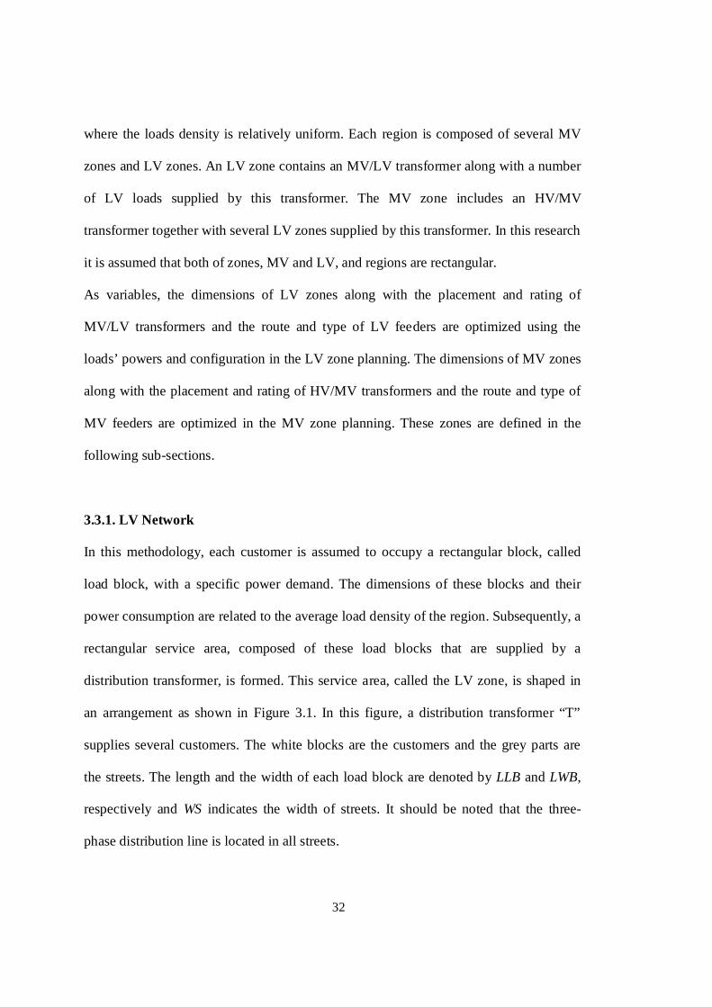
3.3.1. LV Network
In this methodology, each customer is assumed to occupy a rectangular block, called
load block, with a specific power demand. The dimensions of these blocks and their
power consumption are related to the average load density of the region. Subsequently, a
rectangular service area, composed of these load blocks that are supplied by a
distribution transformer, is formed. This service area, called the LV zone, is shaped in
an arrangement as shown in Figure 3.1. In this figure, a distribution transformer “T”
supplies several customers. The white blocks are the customers and the grey parts are
the streets. The length and the width of each load block are denoted by LLB and LWB,
respectively and WS indicates the width of streets. It should be noted that the three-
phase distribution line is located in all streets.

33
Figure 3.1. Typical distribution transformer service area (LV Zone)
The aim is to find the length and width of the LV zones along with the LV feeders’
types and routes and the transformer size and location as the variables to minimize the
total cost per load block (or per unit area). The objective function for LV planning
problem is the cumulative cost of the transformer, LV and MV feeders, and line loss.
Note that the length and thus the cost of the MV feeders are partly determined by the
dimensions of the LV zone. The reliability cost is not incorporated into the LV zone
planning since the cost benefit obtained from reducing outages for some loads in an LV
zone is usually much lower than the cost of required switches.
3.3.2. MV Network
After finding the dimensions of the LV zones and corresponding transformer size, a
rectangular zone is allocated to a distribution substation for optimization of the MV
system. This rectangular zone, called MV zone, is composed of LV zones. Figure 3.2

34
shows an MV zone when all LV zones belong to a single load density region. In this
figure, TLB and TWB are the length and the width of each LV zone. Transformers and
substations are shown by “T” and “SS”, respectively.
Figure 3.2. Typical distribution substation service area (MV Zone)
The values of TLB and TWB are known since they are the output of the LV zone
planning program.
TLB = LLB × HNLB (3.8)
TWB = (LWB + 0.5 × WS) × VNLB (3.9)
where HNLB and VNLB are the number of load blocks supplied by each distribution
transformer in the horizontal and vertical axes which have been optimized in the LV
zone planning section, respectively.
The location and size of substations and MV feeders’ types and routes in addition to the
length and width of the MV zones are as the variables in the MV zone planning
procedure. The objective function is composed of the loss cost, the reliability cost as

35
well as the capital cost for HV/MV transformers and MV feeders per unit area. Here
only the SAIDI and SAIFI contribution from the feeder faults is considered. The bus
voltage level and the feeder current constraints should be satisfied in both LV and MV
zones.
3.4. Implementation of DPSO for PDS Problem
3.4.1. Overview of PSO
PSO is a population-based and self adaptive technique introduced originally by Kennedy
and Eberhart in 1995 [122]. This algorithm handles a population of individuals in
parallel to search capable areas of a multi-dimensional space where the solution is
searched. The individuals are called particles and the population is called a swarm.
Particles as the variables are updated during the optimization procedure [51]. In DPSO,
as the discrete version of PSO, the solution can be reached by rounding off the actual
particle value to the nearest integer during the iterations. In [51], it is mentioned that the
performance of the DPSO is not influenced by this rounding of process. Note that the
continuous methods perform the rounding after the convergence of the algorithm, while
in DPSO, it is applied to all particles in each iteration.
3.4.2. Methodology for Optimization of the PDS Problem
In the PDS problem, the particles are composed of the variables associated with the LV
zones and MV zones. Dimensions of LV zones, distribution transformer sizes and
locations, and the LV feeders’ types and routes are the particles associated with the LV
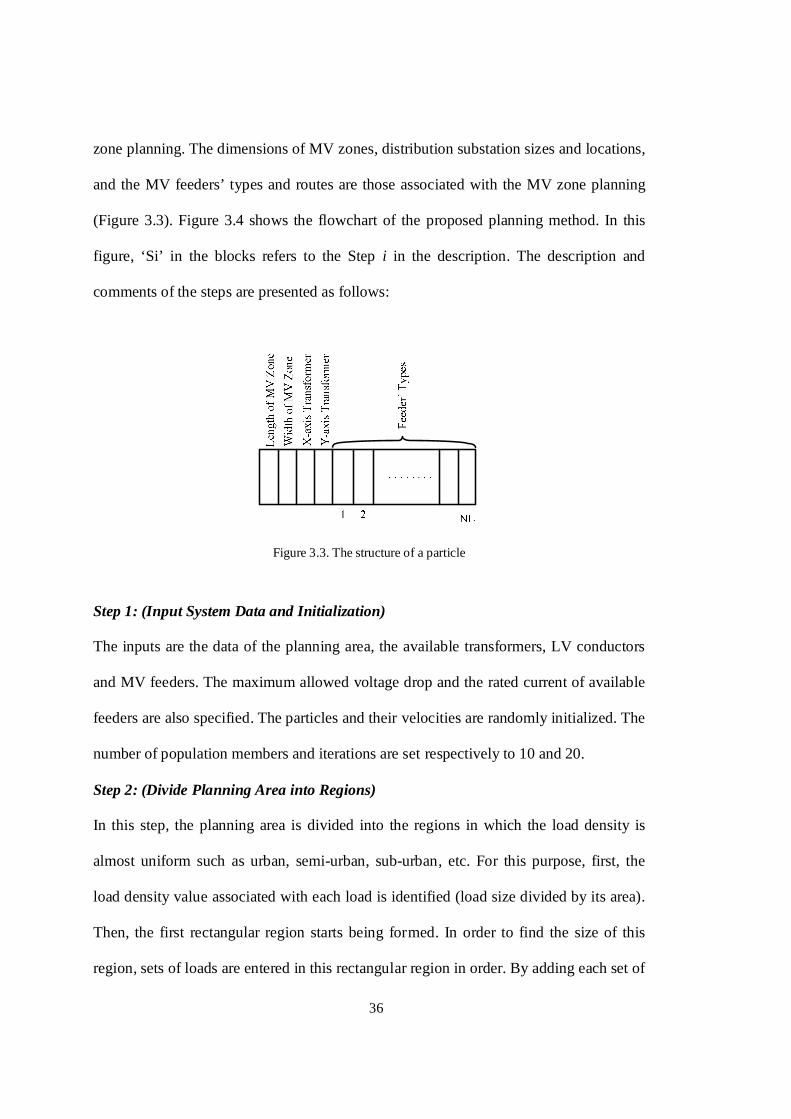
36
zone planning. The dimensions of MV zones, distribution substation sizes and locations,
and the MV feeders’ types and routes are those associated with the MV zone planning
(Figure 3.3). Figure 3.4 shows the flowchart of the proposed planning method. In this
figure, ‘Si’ in the blocks refers to the Step i in the description. The description and
comments of the steps are presented as follows:
Figure 3.3. The structure of a particle
Step 1: (Input System Data and Initialization)
The inputs are the data of the planning area, the available transformers, LV conductors
and MV feeders. The maximum allowed voltage drop and the rated current of available
feeders are also specified. The particles and their velocities are randomly initialized. The
number of population members and iterations are set respectively to 10 and 20.
Step 2: (Divide Planning Area into Regions)
In this step, the planning area is divided into the regions in which the load density is
almost uniform such as urban, semi-urban, sub-urban, etc. For this purpose, first, the
load density value associated with each load is identified (load size divided by its area).
Then, the first rectangular region starts being formed. In order to find the size of this
region, sets of loads are entered in this rectangular region in order. By adding each set of

37
loads, the ‘Relative Standard Deviation’ index (%RSD) of the load density value of
loads is calculated. This index is defined as the Standard Deviation divided by the
Average. If this value is less than a separation rate, the next set of loads is added.
Otherwise, this new set of loads are entered the second region. This collection continues
till all the loads located in the planning area are lumped in regions. The separation rate
depends on many factors such as the size of the planning area. For example it may be
true that separated private houses have a %RSD between 2 and 3 but that high rise
apartments have a %RSD of 10. This would thus give a clear separation of categories.
Figure 3.4. Overall iteration process linking LV-MV optimization

38
Step 3: (Find Average Load Density in each Region)
Regarding the loads located in each region, the average load density corresponding with
each region is calculated. Using the average load density and average size of the load
blocks in each region, the LV zone dimensions (the number of streets and the number of
blocks in each street) will be calculated optimally as shown in Step 4.
Step 4: (Plan LV Networks Assuming Uniform Load Density)
Assuming uniform load density, it is clear that the minimum voltage in an LV zone is
found for the farthest customer load. This voltage depends on the distance between the
transformer and the farthest load. To reduce the voltage drop, this distance should be
reduced. Therefore, the transformer should be located in the centre of the LV zone as
shown in Figure 3.1.
DPSO is employed for optimizing the dimensions of LV zones in this step. The
objective function is the cumulative cost of the MV/LV transformer, LV and MV
feeders, and line loss cost. It should be noted that the length and thus the cost of the MV
feeders are partly determined by the dimensions of the LV zone. For each region, the
dimensions of LV zones as variables are specified as particle N1R in the optimization
process.
]VNLB,HNLB[1N RRR =
where HNLBR and VNLBR are the number of load blocks in the horizontal and vertical
axes in region R, respectively. Since HNLBR and VNLBR are discrete, they are rounded
to the nearest integers.
Since the planning area and the loads in a region are assumed to be completely uniform
in this step, the size and location of distribution transformer and the conductors’ types

39
and routes can be found from the dimensions of the LV zone. Given the number of load
blocks in the horizontal and vertical axes, a rectangular zone is created and the
distribution supply is implemented as shown in Figure 3.1.
The area of LV zone can be simply calculated as:
ALV = (HNLB × LLB) × (VNLB × (LWB + 0.5 × WS)) (3.10)
where ALV is the area of the LV zone in km2. The transformer size and the LV
conductor length are determined as given in (3.11) and (3.12).
STrans = (HNLB × VNLB) × PLoad (3.11)
LLV = ((HNLB – 1) × LLB) × NS (3.12)
where STrans and PLoad are the rating of transformer and the load demand per area. LLV
is the total length of LV conductors required for supplying the load blocks. NS is the
number of streets supplied by a transformer. The length of required MV feeder to supply
the distribution transformer is also calculated by multiplying VNLB and LWB. It should
be noted that the type of MV feeder is already known from previous steps.
To calculate the line losses and evaluate the optimization constraints, the bus voltages
need to be calculated. For this purpose, an admittance matrix is formed using the current
number of the load blocks as well as the transformer and LV conductor impedances. It
should be noted that the impedance model is used for the loads. To calculate the bus
voltage, the following equation can be used only if the Ibus is known.
busbusbusbus1
busbus I.ZVI.YV =⇒= − (3.13)
where the dimensions of V, I and Y depend on the number of load blocks. It should be
noted that the dimensions of the Ybus matrix change during the optimization procedure
since different dimensions of LV zones are generated by each particle. Since there is no

40
current injection (sources) in any of the buses except bus 1, the bus voltages can be
calculated as:
)1(I.)i,1(Z)i(V busbusbus = (3.14)
In this expression, Vbus(i) is the voltage of bus i and Ibus(1) is the injecting current to bus
1. Ibus(1) is calculated using the network power and the voltage of the MV side of the
distribution transformer which is assumed to be set by the transformer tap as 1.03 pu.
Calculating the non-zero element of Ibus, Ibus(1), the voltage at all the buses are found
using (3.14). The line current can be calculated when the bus voltages and feeder
impedances are known. An iterative-based procedure is employed to determine the
lowest cost LV conductor types which maintain the bus voltage within the standard
level.
Step 5: (Is Load Density Close to Uniform?)
If the load density in the planning area is close to uniform, the program continues to the
next step to plan the MV networks for uniform load density. Otherwise, the program
goes to step 7 for applying the non-uniform density condition to the LV zones resulting
from Step 4. It should be noted that the criteria for uniform load density is that the
%RSD of the load density value of the loads in the planning area is less than the
separation rate.
Step 6: (Plan MV Networks for Uniform Load Density)
In this step, there are two variables: the length and width of the MV zone. Similar to the
transformer placement in the LV zone planning for uniform load density, a distribution
substation is situated in the centre of the MV zone to supply the distribution
transformers, and thus their related load blocks, as shown in Figure 3.2. DPSO is

41
employed for optimizing the length and width of the MV zones. The objective function
is composed of the capital cost, loss cost and reliability cost per unit area. The bus
voltage level and the feeder current are included in the objective function as constraints.
The particle N1, composed of the number of LV zones in the horizontal and vertical
axes, is used in DPSO as follows:
]VNTB,HNTB[1N =
where HNTB and VNTB are the number of LV zones located on the horizontal and
vertical axes respectively. Since these are discrete values, they are rounded to the
nearest integers. The total number of blocks is calculated by multiplying HNTB and
VNTB. Since the MV zone is rectangular, the MV zone area is
AMV = (HNTB × VNTB) × OALV (3.15)
where AMV is the area of MV zone in (km2). OALV is the LV zone area, resulting from
Step 4.
To calculate the cost of substation and MV feeder as parts of the objective function in
the MV zone planning, the rating of substation and length of MV feeder need to be
calculated.
SSubs = (HNTB × VNTB) × OSTrans (3.16)
LMV = (TLB × HNTB) – TWB (3.17)
where SSubs and OSTrans are the rating of substation and the transformer rating calculated
from the LV zone planning (Step 4) respectively and LMV is the length of the MV
feeder. Similar to the LV zone planning, an iterative procedure is used to determine the
MV feeder types as the optimization constraints are met.

42
It should be noted that the configuration of both MV and LV zones are like the letter
“H” as observed in Figures 3.1 and 3.2. As a result, they are called the H-type
configuration. Another configuration, called Branch-type, is considered in section 3.5.1.
The minimum bus voltage is calculated using (3.13) and (3.14) following the same
procedure as used in the LV zone planning (Step 4). Note that the substation voltage is
set as 1.03 pu. After finalizing this step, the program goes to Step 9.
Step 7: (Plan LV Networks for Non-Uniform Load Density)
In this step, the non-uniform condition is applied to the LV zones resulting from Step 4.
For this purpose, the uniform load blocks, located in an LV zone, are replaced with
realistic loads (realistic placement and size), while the LV zone dimensions are kept the
same as identified in Step 4. After that, the placement and size of distribution
transformers and LV conductors’ types in the LV zone are considered as the variables,
particle N2R in DPSO, and are optimized to minimize the objective function.
]LCNC.,..,2LC,1LC,YDTL,XDTL[2N RRRRRR =
XDTLR and YDTLR are the location of distribution transformer on horizontal and
vertical axes in region R, respectively. LCiR is the type of LV conductor i in region R.
NC is the number of required different LV conductors in an LV zone.
For LV network, when some portions of the planning area cannot be approximated by a
complete rectangle such as having an obstacle like a lake, a complete rectangle is
formed as if no obstacle exists (the size of the rectangle is determined from step 4).
After that, a zero power is assigned to the load blocks located in the part of this
rectangle in which the obstacle is situated.
To allocate a distribution transformer, the following points should be noted:

43
1. If the location of transformer is within one of the load blocks, it should be changed to
the nearest street (Figure 3.1).
2. If the location of transformer is in the middle of a street, it should be moved to one
side of the street.
3. If the location of transformer is on an obstacle, it should be moved to the nearest
feasible point.
In this step, the bus voltages are determined using (3.13) and (3.14) similar to Step 4.
Step 8: (Plan MV Networks for Non-Uniform Load Density)
In this step, in addition to the length and width of the MV zone, the HV/MV substation
size and location, and the MV feeders’ types and routes are included as the variables.
Similar to Step 6, the objective function is composed of the capital cost, loss cost and
reliability cost per unit area and the constraints are the bus voltage level and the feeder
current (calculated using (3.13) and (3.14)). The particle N2, used in the employed
DPSO, is composed of the number of LV zones in the horizontal and the vertical axes,
the rating and location of substation, and the type of MV feeders in the corresponding
MV zone (see Figure 3.3).
]MFNF.,..,2MF,1MF,YDSL,XDSL[2N =
where XDSL and YDSL are the location of distribution substation on horizontal and
vertical axes, respectively. MFi is the type of MV feeder i. NF is the number of required
different MV feeders in an MV zone.
Step 9: (MV Construction Type Change?)
Since the MV feeder cost is the common element in the total cost associated with LV
and MV zones, the optimized MV feeder types, obtained in Step 6 or 8, are compared
44
with those used in the planning of the LV zone (Step 4 or 7). If they are the same, the
program is terminated and the final results are printed. Otherwise, the program continues
from Step 4 in the next iteration and the LV zone planning is implemented based on the
MV feeders’ types resulted from the current MV zone planning (Step 6 or 8).
3.5. Results
Two different cases are evaluated in this section. In the first case, it is assumed that both
MV and LV zones are planned in a uniform load density region. In the second case, the
non-uniform load density conditions applied in order to make the solution more realistic.
3.5.1. Uniform Load Density Based Case
The planning approach is tested on an area, the characteristics of which are listed in
Table 3.1. Two configurations are investigated in this case: the H-type and the Branch-
type configurations (Figures 3.2 and 3.5). The main benefit of the H-type configuration
over the Branch type is its low total capital cost. However, it suffers from higher
reliability cost. Selection between these two configurations depends on the reliability
weight factors.
To compare the performance of DPSO, both GA and NLP are also applied to the PDS
problem. The population size and the generation number for GA are selected 10 and 20
respectively similar to those used for DPSO. Other parameters in GA are selected
similar to those defined as default in ‘GAtool’ in Matlab. In the studies performed, the
NLP converges to local minima for some starting points. It should be noted that the
DPSO results are also compared with those obtained with an exhaustive search method
and they are found to be identical. In computer science, exhaustive search or brute-force

45
search, also known as generate and test, is a technique which consists of systematically
enumerating all possible candidates for the solution. Performance comparisons of DPSO
with GA are given in Tables 3.2 to 3.4. Tables 3.5 and 3.6 give the list of available
transformers and LV and MV feeders along with their characteristics.
Table 3.1. Characteristics of the test system
Parameter Value
Load Power 2.5 (kW)
Length of Load Block 20 m
Width of Load Block 20 m
Width of Street 10 m
Base LV Voltage 415 (V)
Base MV Voltage 33 (kV)
Power Factor 0.8
Failure Rate 0.1864 (fault/km.yr)
Load Impedance 44 + j 33 (Ω)
kPL 168000 $/MW
kL 4 ¢/kWh
lsf 0.3
r 0.07
T 20 years
CID 0.02 ($/min)
CIN 6 ($/interruption)
Switching Time 30 minutes
Repair Time 90 minutes

46
260 m
. . . .
Figure 3.5. The optimized MV zone in Branch-type configuration
The reliability parameters are selected based on [48,49]. The planning is performed for
peak load power (2.5 kW per block) and the upper voltage limit of 1.03 pu is chosen
such that the low load voltage does not rise above 1.05 pu due to the Ferranti effect. The
acceptable voltage drops in the MV and LV sides are assumed to be 97% and 95%,
respectively [14,41]. Based on a sample load duration curve used in [14], the loss factor
is assumed to be 0.35. The coding is written in Matlab 7.6 programming language and is
executed in a desktop computer with the features as Core 2 Due CPU, 2.66 GHz, and 2
GB of RAM.
Based on the dimensions of load blocks and their power demand, the average load
density is found to be 5 MW/km2. Solving the LV zone planning, the solution is that
each transformer should supply 3 streets (i.e., 78 blocks). The transformer size,
calculated by (3.11), is 195 kVA. Using the available transformers listed in Table 3.5,
the transformer rating is selected as 200 kVA. Using (3.10), the rectangular LV zone
area is obtained as 0.039 km2. Table 3.2 gives a summary of the LV zone planning
outputs. It should be noted that the costs mentioned in Table 3.2 and all other tables are
the cost per block.
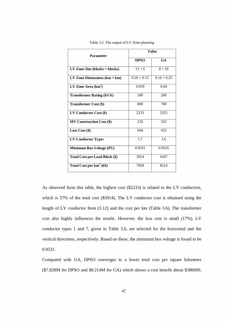
47
Table 3.2. The output of LV Zone planning
Parameter Value
DPSO GA
LV Zone Size (blocks × blocks) 13 × 6 8 × 10
LV Zone Dimensions (km × km) 0.26 × 0.15 0.16 × 0.25
LV Zone Area (km2) 0.039 0.04
Transformer Rating (kVA) 200 200
Transformer Cost ($) 800 780
LV Conductor Cost ($) 2233 2323
MV Construction Cost ($) 216 352
Loss Cost ($) 664 652
LV Conductor Types 1,7 1,6
Minimum Bus Voltage (PU) 0.9531 0.9535
Total Cost per Load Block ($) 3914 4107
Total Cost per km2 (k$) 7828 8214
As observed from this table, the highest cost ($2233) is related to the LV conductors,
which is 57% of the total cost ($3914). The LV conductor cost is obtained using the
length of LV conductor from (3.12) and the cost per km (Table 3.6). The transformer
cost also highly influences the results. However, the loss cost is small (17%). LV
conductor types 1 and 7, given in Table 3.6, are selected for the horizontal and the
vertical directions, respectively. Based on these, the minimum bus voltage is found to be
0.9531.
Compared with GA, DPSO converges to a lower total cost per square kilometer
($7.828M for DPSO and $8.214M for GA) which shows a cost benefit about $386000.

48
Furthermore, the exhaustive search method shows identical results with the proposed
algorithm at the expense of longer computation time. In this case, the proposed DPSO
converges quickly within 10 iterations.
After receiving the outputs of LV zone planning, the transformer characteristics and the
dimensions of LV zone are considered as the inputs of MV zone planning. Then, a
similar procedure is applied for the MV zone planning as in the case of H-type
configuration. Table 3.3 illustrates the results of MV zone planning.
Table 3.3. The output of MV Zone planning for H-type configuration
Parameter Value
DPSO GA
MV Zone Size (blocks × blocks) 5 × 15 9 × 8
MV Zone Dimensions (km × km) 1.3 × 2.25 2.34 × 1.2
MV Zone Area (km2) 2.925 2.808
Substation Rating (MVA) 15 15
Substation Cost (k$) 43.89 45.72
MV Construction Cost (k$) 8.66 9.01
MV Construction Type 1 1
Reliability Cost (k$) 11.35 11.45
SAIDI (min) 41.45 48.25
SAIFI 2.15 2.15
Loss Cost (k$) 2.71 3.75
Minimum Bus Voltage (PU) 0.9776 0.9795
Total Cost per Block (k$) 66.61 69.94
Total Cost per km2 (k$) 1708 1793

49
The MV zone planning results in 5 blocks in the horizontal axis and 15 blocks in the
vertical axis. With these, the area of MV zone is calculated using (3.15) as 2.925 km2.
Given the number of LV zones located in the MV zone, the substation rating is
calculated using (3.16) as 15 MVA. As shown in Table 3.3, the rating 15 MVA is
selected as the HV/MV transformer size. Compared with the LV zone planning in which
the LV conductor cost is the main cost, the substation cost is the major cost of k$43.89
in the MV zone planning, which is 66% of the total cost. Similar to the LV zone, the
loss cost is small compared with the other costs.
The SAIDI and SAIFI are found to be 41.45 minutes and 2.15, respectively. This
calculation is based on the assumption that the sectionalizing switches are located on
both ends of each primary branch and a circuit breaker is at the beginning of each main
lateral (Figure 3.2). Similar to the LV zone planning, the minimum bus voltage is found
near the boundary value of 0.97 using the lowest cost MV feeders to satisfy the
constraints.
It should be noted that after applying the exhaustive search, similar results were
obtained and this illustrates the accuracy of the employed DPSO, albeit faster
convergence time. Compared with GA, total cost per LV block obtained by DPSO is
about $3300 (≈$85000 per square kilometer) less than GA as seen in Table 3.3. All
these results are based on the H-type configuration zones.
In order to improve the reliability index, another structure called Branch-type
configuration is applied to the proposed planning. In this type of configuration, each
substation is connected directly to the nearest distribution transformer as shown in
Figure 3.5. Table 3.4 illustrates the outputs of MV zone planning for the Branch-type

50
configuration. The trend of MV zone dimensions from first iteration to the last iteration
is shown in Figure 3.6. Table 3.4 gives costs obtained by DPSO and GA. An exhaustive
search method is also employed for this problem that gives identical results with the
DPSO method.
Figure 3.6. Number of blocks in horizontal and vertical axes in Branch-type configuration
The proposed iterative method for optimizing both LV and MV zones (Figure 3.4) in the
Branch type configuration is assessed. For this purpose, the exhaustive search method is
applied to both LV and MV zones. To apply the exhaustive search method, the objective
function for all combinations of LV zone dimensions and MV zone dimensions should
be calculated. For example, assume that an LV zone side cannot include more than 19
load blocks (because of the voltage drop constraint) and an MV zone side cannot include
more than 35 LV zones. The number of states will be 19 × 19 × 35 × 35= 442225. The
running time for calculating the objective function is about 4 seconds. Therefore, the
total required time for the exhaustive search method will be at least 20 days. This
2 4 6 8 10 12 14 16 18 200
5
10
15
20
25
30
35
Iteration Number
Nu
mb
er
Number ofLV Zones in Horizontal Axis
Number ofLV Zones in Vertical Axis
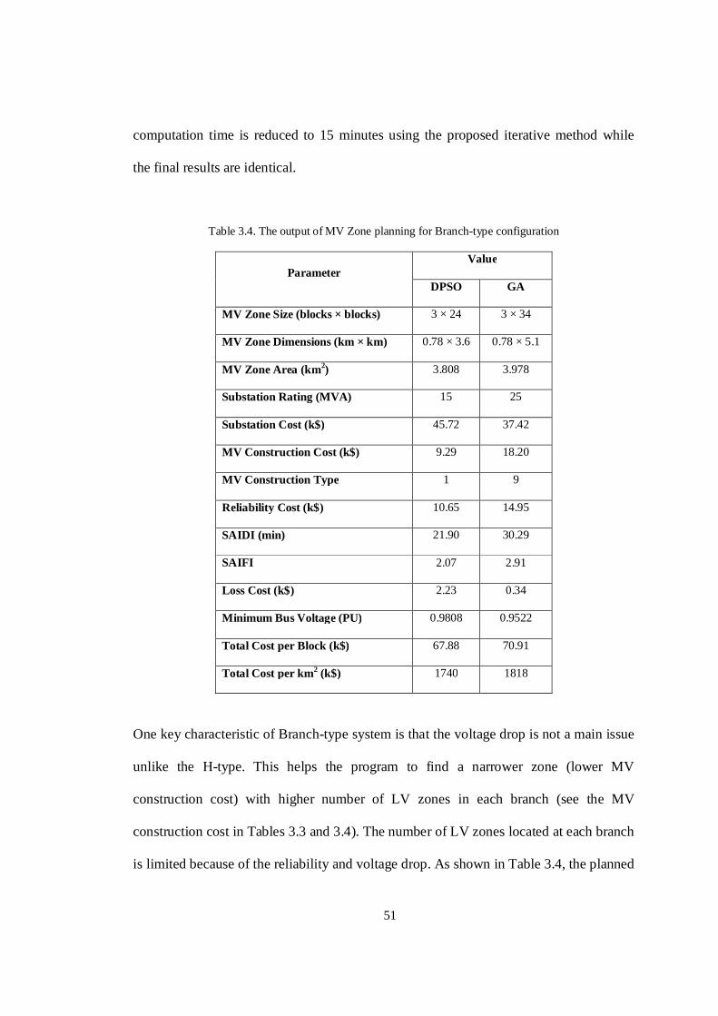
51
computation time is reduced to 15 minutes using the proposed iterative method while
the final results are identical.
Table 3.4. The output of MV Zone planning for Branch-type configuration
Parameter Value
DPSO GA
MV Zone Size (blocks × blocks) 3 × 24 3 × 34
MV Zone Dimensions (km × km) 0.78 × 3.6 0.78 × 5.1
MV Zone Area (km2) 3.808 3.978
Substation Rating (MVA) 15 25
Substation Cost (k$) 45.72 37.42
MV Construction Cost (k$) 9.29 18.20
MV Construction Type 1 9
Reliability Cost (k$) 10.65 14.95
SAIDI (min) 21.90 30.29
SAIFI 2.07 2.91
Loss Cost (k$) 2.23 0.34
Minimum Bus Voltage (PU) 0.9808 0.9522
Total Cost per Block (k$) 67.88 70.91
Total Cost per km2 (k$) 1740 1818
One key characteristic of Branch-type system is that the voltage drop is not a main issue
unlike the H-type. This helps the program to find a narrower zone (lower MV
construction cost) with higher number of LV zones in each branch (see the MV
construction cost in Tables 3.3 and 3.4). The number of LV zones located at each branch
is limited because of the reliability and voltage drop. As shown in Table 3.4, the planned
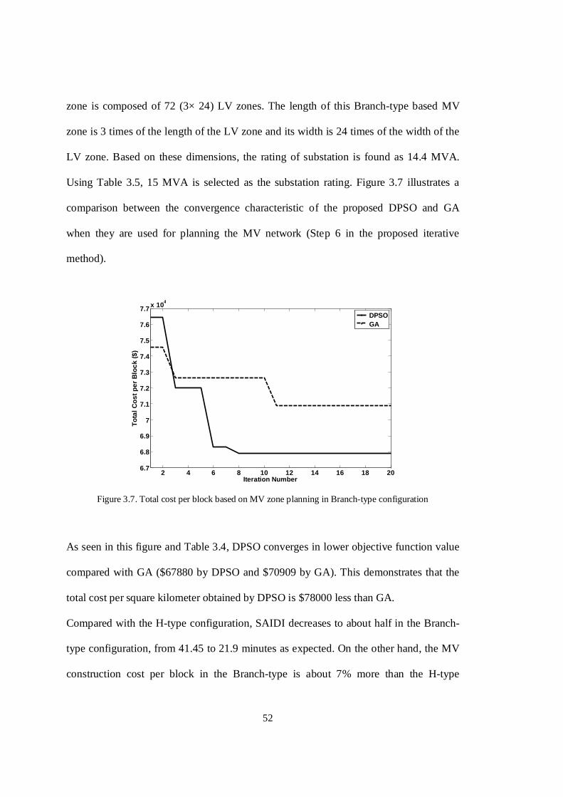
52
zone is composed of 72 (3× 24) LV zones. The length of this Branch-type based MV
zone is 3 times of the length of the LV zone and its width is 24 times of the width of the
LV zone. Based on these dimensions, the rating of substation is found as 14.4 MVA.
Using Table 3.5, 15 MVA is selected as the substation rating. Figure 3.7 illustrates a
comparison between the convergence characteristic of the proposed DPSO and GA
when they are used for planning the MV network (Step 6 in the proposed iterative
method).
Figure 3.7. Total cost per block based on MV zone planning in Branch-type configuration
As seen in this figure and Table 3.4, DPSO converges in lower objective function value
compared with GA ($67880 by DPSO and $70909 by GA). This demonstrates that the
total cost per square kilometer obtained by DPSO is $78000 less than GA.
Compared with the H-type configuration, SAIDI decreases to about half in the Branch-
type configuration, from 41.45 to 21.9 minutes as expected. On the other hand, the MV
construction cost per block in the Branch-type is about 7% more than the H-type
2 4 6 8 10 12 14 16 18 206.7
6.8
6.9
7
7.1
7.2
7.3
7.4
7.5
7.6
7.7 x 10⁴
Iteration Number
To
tal C
ost
per
Blo
ck (
$)
DPSO GA
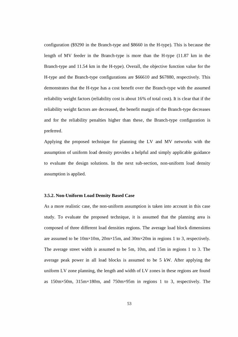
53
configuration ($9290 in the Branch-type and $8660 in the H-type). This is because the
length of MV feeder in the Branch-type is more than the H-type (11.87 km in the
Branch-type and 11.54 km in the H-type). Overall, the objective function value for the
H-type and the Branch-type configurations are $66610 and $67880, respectively. This
demonstrates that the H-type has a cost benefit over the Branch-type with the assumed
reliability weight factors (reliability cost is about 16% of total cost). It is clear that if the
reliability weight factors are decreased, the benefit margin of the Branch-type decreases
and for the reliability penalties higher than these, the Branch-type configuration is
preferred.
Applying the proposed technique for planning the LV and MV networks with the
assumption of uniform load density provides a helpful and simply applicable guidance
to evaluate the design solutions. In the next sub-section, non-uniform load density
assumption is applied.
3.5.2. Non-Uniform Load Density Based Case
As a more realistic case, the non-uniform assumption is taken into account in this case
study. To evaluate the proposed technique, it is assumed that the planning area is
composed of three different load densities regions. The average load block dimensions
are assumed to be 10m×10m, 20m×15m, and 30m×20m in regions 1 to 3, respectively.
The average street width is assumed to be 5m, 10m, and 15m in regions 1 to 3. The
average peak power in all load blocks is assumed to be 5 kW. After applying the
uniform LV zone planning, the length and width of LV zones in these regions are found
as 150m×50m, 315m×180m, and 750m×95m in regions 1 to 3, respectively. The
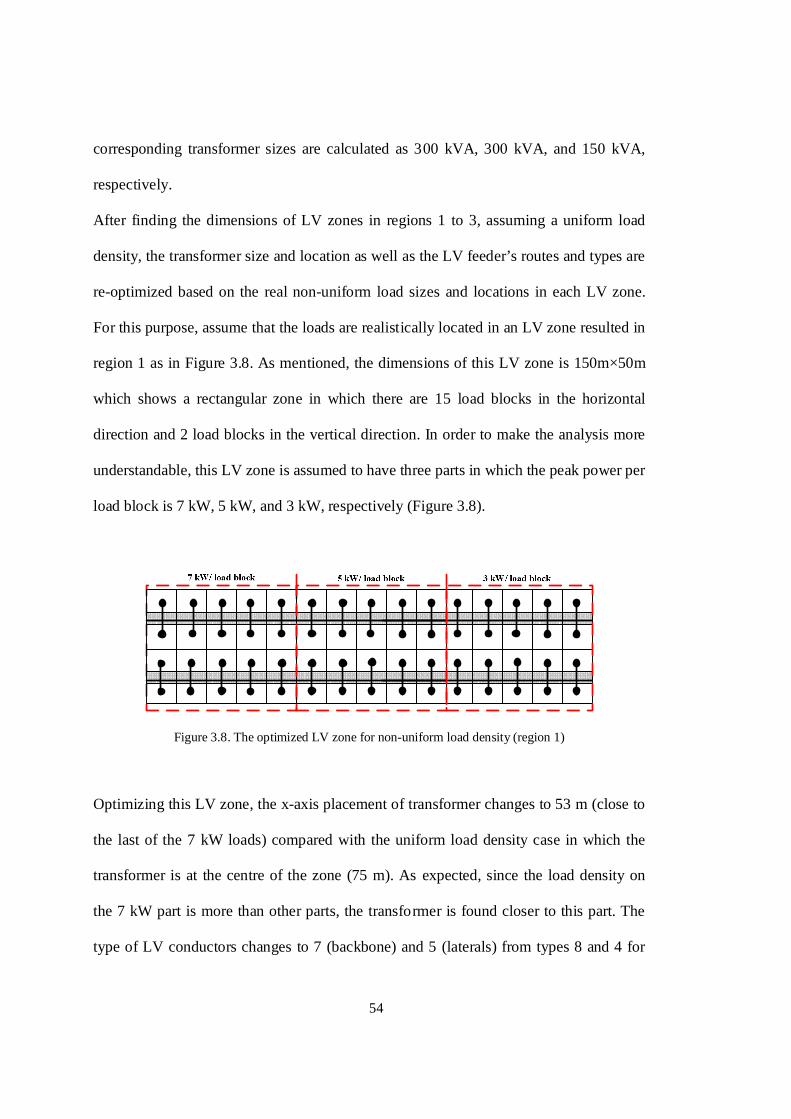
54
corresponding transformer sizes are calculated as 300 kVA, 300 kVA, and 150 kVA,
respectively.
After finding the dimensions of LV zones in regions 1 to 3, assuming a uniform load
density, the transformer size and location as well as the LV feeder’s routes and types are
re-optimized based on the real non-uniform load sizes and locations in each LV zone.
For this purpose, assume that the loads are realistically located in an LV zone resulted in
region 1 as in Figure 3.8. As mentioned, the dimensions of this LV zone is 150m×50m
which shows a rectangular zone in which there are 15 load blocks in the horizontal
direction and 2 load blocks in the vertical direction. In order to make the analysis more
understandable, this LV zone is assumed to have three parts in which the peak power per
load block is 7 kW, 5 kW, and 3 kW, respectively (Figure 3.8).
Figure 3.8. The optimized LV zone for non-uniform load density (region 1)
Optimizing this LV zone, the x-axis placement of transformer changes to 53 m (close to
the last of the 7 kW loads) compared with the uniform load density case in which the
transformer is at the centre of the zone (75 m). As expected, since the load density on
the 7 kW part is more than other parts, the transformer is found closer to this part. The
type of LV conductors changes to 7 (backbone) and 5 (laterals) from types 8 and 4 for

55
the uniform case. It should be noted that because of practical reasons, no more than 2
types of conductors are allowed to be used in a zone.
For MV zone planning, it is assumed that the length of region 1 is 900 m, the length of
region 2 is 1260 m, and the length of region 3 is unlimited. The width of regions is also
assumed to be unlimited. After applying the MV zone planning, a substation with the
rating of 15 MVA is found to be located at 1451 m and 150 m in x and y axes (Figure
3.9). The length and width of MV zone is determined to be 5160 m and 300 m.
Figure 3.9. The optimized MV zone for non-uniform load density (not to scale)
As observed, the substation location is not in the centre of the MV zone since the load
density is not uniform in the resulted MV zone and as expected the location of
substation is found closer to the region with higher load density. The type of feeders for
all load densities is found to be type 1. Figure 3.9 shows the configuration of MV zone
after planning based on the non-uniform load density assumption.

56
A comparison between the convergence characteristic of the proposed DPSO and GA
for MV zone planning (Step 8 in the iterative method) in this non-uniform load density
based case is illustrated in Figure 3.10. As observed, DPSO converges in lower total
cost per square kilometer rather than GA ($1.035M by DPSO and $1.092M by GA).
Figure 3.10. Total cost per square kilometer based on MV zone planning in case 2
Tables 3.5 show the characteristics of available MV/LV and HV/MV transformers such
as the impedance, the capital cost, and the operation and maintenance cost. These
characteristics along with the rated current associated with the available LV and MV
feeders are given in Table 3.6.
3.6. Summary
A new methodology is introduced in this chapter for integrated planning of MV and LV
segments of a distribution system optimally considering feeder types and routes, as well
as, transformer ratings and placements. The objective function associated with the LV
2 4 6 8 10 12 14 16 18 201
1.05
1.1
1.15
1.2
1.25
1.3
1.35
1.4 x 10⁶
Iteration Number
To
tal C
ost
per
km
2 ($
)
DPSO GA

57
segment planning is composed of the loss cost as well as the total capital cost for
MV/LV transformers, LV conductors, and the part of the MV feeders located in an LV
zone. The objective function associated with the MV segment planning consists of the
reliability cost, the line loss cost and the total capital cost for HV/MV transformers and
MV feeders. The voltage drop and the feeder current are considered as constraints in
planning both LV and MV segments.
DPSO is employed iteratively to solve the integrated distribution planning problem. The
results are compared with those obtained by NLP, GA and the exhaustive search
method. NLP as an analytical method could not improve the initial values due to the
high discreteness of the problem. The proposed algorithm illustrates higher accuracy in
all cases compared with GA for similar expected computational effort. Also the results
of the DPSO have been compared with the exhaustive search method and are found to
be identical. However, the exhaustive search is more time consuming.
A low computational effort iterative based technique is proposed for planning both LV
and MV networks altogether. The results are found to be identical with those obtained
by the exhaustive search. This illustrates the high accuracy of the proposed technique. It
is shown that the proposed technique can be employed for planning of both uniform and
non-uniform load densities. The proposed method can provide guidance for planning of
practical MV and LV distribution systems.
58
Table 3.5. The characteristics of available transformers
Elements Impedance Capital
Cost
O&M
Cost
Transformers
(kVA) Ω (PU) k$ $/year
25 0.006+0.017 i 10 300
30 0.006+0.018 i 12.3 311
50 0.005+0.018 i 16.8 325
63 0.005+0.019 i 18.5 348
100 0.005+0.021 i 22 376
150 0.005+0.022 i 24.8 408
200 0.003+0.022 i 26.3 455
250 0.005+0.023 i 37 503
300 0.004+0.024 i 40.2 564
350 0.004+0.022 i 45.7 607
Substation
(MVA) Ω (PU) M$ $/year
3 0.040 i 1.6 16000
8 0.045 i 2.47 16800
15 0.045 i 3.1 18100
25 0.055 i 3.6 20500
30 0.060 i 3.8 23700
50 0.065 i 4.1 28000

59
Table 3.6. The characteristics of available feeders
Elements Impedance Current
Rating
Capital
Cost
O&M
Cost
MV
Feeders (Ω) (A) k$/km $/year/km
No. 1 1.75 + j 0.100 198 52 405
No. 2 1.40 + j 0.100 212 53 553
No. 3 1.00 + j 0.100 232 54.5 695
No. 4 0.90 + j 0.080 275 56.7 821
No. 5 0.75 + j 0.050 332 60 940
No. 6 0.63 + j 0.090 300 68.5 1042
No. 7 0.47+ j 0.087 386 76 1122
No. 8 0.30 + j 0.080 486 86 1197
No. 9 0.15 + j 0.076 601 100 1258
LV
Conductor (Ω) (A) k$/km $/year/km
No. 1 2.50 + j 0.200 84 40 255
No. 2 2.20 + j 0.100 96 41.5 364
No. 3 1.90 + j 0.100 110 43 364
No. 4 1.60 + j 0.080 145 45 546
No. 5 1.30 + j 0.050 197 48.5 632
No. 6 0.74 + j 0.080 244 51.5 698
No. 7 0.44 + j 0.070 312 56 749
No. 8 0.25 + j 0.068 387 63 780
No. 9 0.10 + j 0.067 443 75 807

60

61
CHAPTER 4
A New Optimization Method for Planning Problems
4.1. Introduction
Since the size of electrical elements is a discrete value and that the objective elements
have a nonlinear relation with the size of elements, the resulting objective function in
planning problems is nonlinear and discrete. This discreteness and nonlinearity make the
function to have a number of local minima. Therefore, selecting an appropriate
optimization method is a main concern in planning of a distribution network. A reliable
optimization method should have high accuracy and robustness.
In this chapter, a Modified Discrete Particle Swarm Optimization (MDPSO) is
proposed. This method is studied by finding the placement and size of capacitors in a
distribution system. The objective function is composed of the line loss and the
capacitors investment cost. The bus voltage and the feeder current as constraints are
included in the objective function by a constraint penalty factor.
To validate the proposed method, the 18-bus IEEE distribution system and the semi-
urban distribution system which is connected to bus 2 of the Roy Billinton Test System
(RBTS) are used. The proposed method is applied to the problem and its robustness and
accuracy are studied. The results are compared with conventional DPSO, GA, and NLP.
It is illustrated on two examples that the MDPSO is more accurate and particularly more
robust than others for the planning of capacitors.

62
4.2. Problem Formulation
The loads and capacitors are modeled as impedance, a series RL for loads and a
capacitive reactance for capacitors. The objective function and the constraints are also
expressed in this section. Minimizing the total cost of capacitors as well as the
distribution line loss is the main objective of the Allocation and Sizing of Capacitors
(ASC) problem. The bus voltage and the feeder current as constraints are included in the
objective function with a penalty factor. As all of the objective function elements are
simply converted into the composite equivalent cost, this problem is solved using a
single-objective optimization method. The objective function is defined as (3.1) in
which CI is zero. In this equation, CCAP and CO&M are the capital cost and the operation
and maintenance cost of capacitors. The line loss is converted into an equivalent cost by
a simplified equation of (4.1) as:
CL = PLoss× kL×8760 (4.1)
The bus voltage and the feeder current should be maintained within standard levels as
given in (3.6) and (3.7).
4.3. Applying Modified DPSO to ASC Problem
The first step in an optimization procedure is identifying the variables. The variables,
particles, in the ASC problem are the size and the placement of capacitors. Figure 4.1
shows the structure of particles in the employed DPSO.
As observed, the particle is composed of NB cells with the value of Ci. Each candidate
bus for installing a capacitor is assigned by a cell and the rating of the capacitor at the
relative candidate bus is the value of the corresponding cell.

63
Figure 4.1. Structure of a particle
For example, Ci is the rating of the capacitor installed at bus i. If all buses are candidates
for installing capacitors, NB will be the number of buses. Therefore, the number of
variables is at most equal to the number of buses. If the value of a cell, the capacitor
size, is more than a specific threshold, it indicates that a capacitor is installed at that bus.
Otherwise, no capacitor is placed at the relative bus. This specific threshold is the
minimum size of the available capacitors.
It will be observed that the results obtained by conventional DPSO are improved when
the crossover and mutation operators are included in DPSO procedure. Furthermore, the
robustness of optimization method is improved by this modification. This is mainly
because these operators increase the diversity of variables. Figure 4.2 shows the
flowchart of the proposed method. The description and comments of the steps are
presented as follows.
Step 1: (Input System Data and Initialization)
In this step, the distribution network configuration and data and the available capacitors
are input. The maximum allowed voltage drop, the characteristics of feeders, impedance
and rated current, are also specified. The DPSO parameters, number of population
members and iterations as well as the PSO weight factors, are also identified. The
random-based initial population of particles Xj (size of capacitors) and the particles
velocity Vj in the search space are also initialized.

64
Step 2: (Calculate the Objective Function)
Given the capacitors size determined in the previous step, the admittance matrix is
reconstructed. Using the new admittance matrix, a load flow program is run and the bus
voltages as well as the feeder currents are calculated. These are used to calculate the
distribution line loss. After that, the objective function is constituted and the constraints
are also computed in this step and included in the objective function with a penalty
factor, (3.1). It means that if a constraint is not satisfied, a large number as a penalty
factor is added to the objective function to exclude the relevant solution from the search
space.
Step 3: (Calculate pbest)
The component of the objective function value associated with the position of each the
particles is compared with the corresponding value in previous iteration and the position
with lower objective function is recorded as pbest for the current iteration.
≥
=++
++
kj
1kj
1kj
kj
1kj
kj1k
jOFOFifx
OFOFifpbestpbest
p
(4.2)
where, k is the number of iterations, and OFj is the objective function component
evaluated for particle j.
Step 4: (Calculate gbest)
In this step, the lowest objective function among the pbests associated with all particles
in the current iteration is compared with it in the previous iteration and the lower one is
labeled as gbest.
≥
= ++
++
k1k1kj
k1kk1k
OFOFifpbest
OFOFifgbestgbest
p
(4.3)

65
Figure 4.2. Algorithm of proposed PSO-based approach
Step 5: (Update position)
The position of particles for the next iteration can be calculated using the current pbest
and gbest as follows:
)Xgbest(randc)Xpbest(randcVV kj
kj2
kj
kj1
kj
1kj −+−+=+ ω (4.4)

66
where kjV is the velocity of particle j at iteration k,ω is the inertia weight factor, ci is the
acceleration coefficients, kjX is the position of particle j at iteration k, k
jpbest is the best
position of particle j at iteration k, and kgbestis the best position among all particles at
iteration k.
As mentioned before, using the available data, ω as inertia weight factor, and c1 and c2
as acceleration coefficients, the velocity of particles is updated. It should be noted that
the acceleration coefficients, c1 and c2, are different random values in the interval [0,1]
and the inertia weight ω is defined as follows:
IterItermax
minmaxmax ×
−−=
ωωωω (4.5)
where ωmax is the final inertia weight factor, ωmin is the initial inertia weight factor, Iter
is the current iteration number, and Itermax is the maximum iteration number.
As observed in (4.5), ω is to adjust the effect of the velocity in the previous iteration on
the new velocity for each particle. Regarding the obtained velocity of each particle by
(4.5), the position of particles can be updated for the next iteration using (4.6).
1kj
kj
1kj VXX ++ += (4.6)
The inertia weight factor is set as 0.9 and both the acceleration coefficients as 0.5.
After this step, half of the population members continue DPSO procedure and other half
goes through the crossover and mutation operators. The first half continues their route at
Step 7 and the second half goes through step 6.
Step 6: (Apply Crossover and Mutation Operators)
In this step, the crossover and mutation operators are applied to the half of the
population members. This is done to increase the diversity of the variables to improve

67
the local minimum problem. Figures 4.3 and 4.4 show the operation of crossover and
mutation operators.
Figure 4.3. A sample crossover operation
Figure 4.4. A sample mutation operation
Step 7: (Check convergence criterion)
If Iter = Itermax or if the output does not change for a specific number of iterations, the
program is terminated and the results are printed, else the program goes to step 2.
4.4. Results
To validate the proposed method, two test systems are studied: the 12.5 kV 18-bus IEEE
distribution system as case 1 and the 11 kV 37-bus distribution system connected to bus
2 of the RBTS as case 2. It is assumed that the energy cost is 6 ¢/kWh. The installation

68
cost of capacitors is assumed to be 4$/kvar and the annual incremental cost is selected
8.75% of the installation cost. The available capacitors are considered as multiple sets of
300 kvar banks. The number of years in the study timeframe is assumed to be 20 years.
To evaluate the proposed method, it is compared with four methods for capacitor
planning, DPSO, GA [17,38,39], SA [48], and DNLP [20]. DPSO is programmed as a
m-file in Matlab. In order to simulate the rest of these optimization methods, the
optimization tool in Matlab, called Optimtool, is used. This tool includes GA and SA,
but for simulating DNLP, ‘fminunc’ [8] and ‘fminsearch’ [9], as NLP solvers in
Optimtool, are modified by quantizing the variables (capacitor rating) in each step.
4.4.1. Case 1
The 12.5 kV 18-bus IEEE distribution system [19,100,123] is modified and used in this
case (Figure 4.5).
Figure 4.5. Single-line diagram of the 18-bus IEEE distribution system
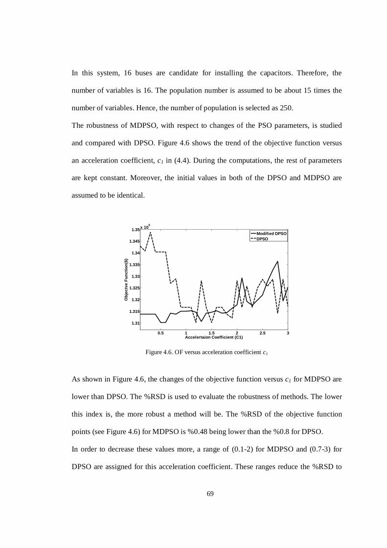
69
In this system, 16 buses are candidate for installing the capacitors. Therefore, the
number of variables is 16. The population number is assumed to be about 15 times the
number of variables. Hence, the number of population is selected as 250.
The robustness of MDPSO, with respect to changes of the PSO parameters, is studied
and compared with DPSO. Figure 4.6 shows the trend of the objective function versus
an acceleration coefficient, c1 in (4.4). During the computations, the rest of parameters
are kept constant. Moreover, the initial values in both of the DPSO and MDPSO are
assumed to be identical.
Figure 4.6. OF versus acceleration coefficient c1
As shown in Figure 4.6, the changes of the objective function versus c1 for MDPSO are
lower than DPSO. The %RSD is used to evaluate the robustness of methods. The lower
this index is, the more robust a method will be. The %RSD of the objective function
points (see Figure 4.6) for MDPSO is %0.48 being lower than the %0.8 for DPSO.
In order to decrease these values more, a range of (0.1-2) for MDPSO and (0.7-3) for
DPSO are assigned for this acceleration coefficient. These ranges reduce the %RSD to
0.5 1 1.5 2 2.5 3
1.31
1.315
1.32
1.325
1.33
1.335
1.34
1.345
1.35x 10⁶
Accelertaion Coefficient (C1)
Ob
ject
ve F
un
ctio
n($
)
Modified DPSODPSO
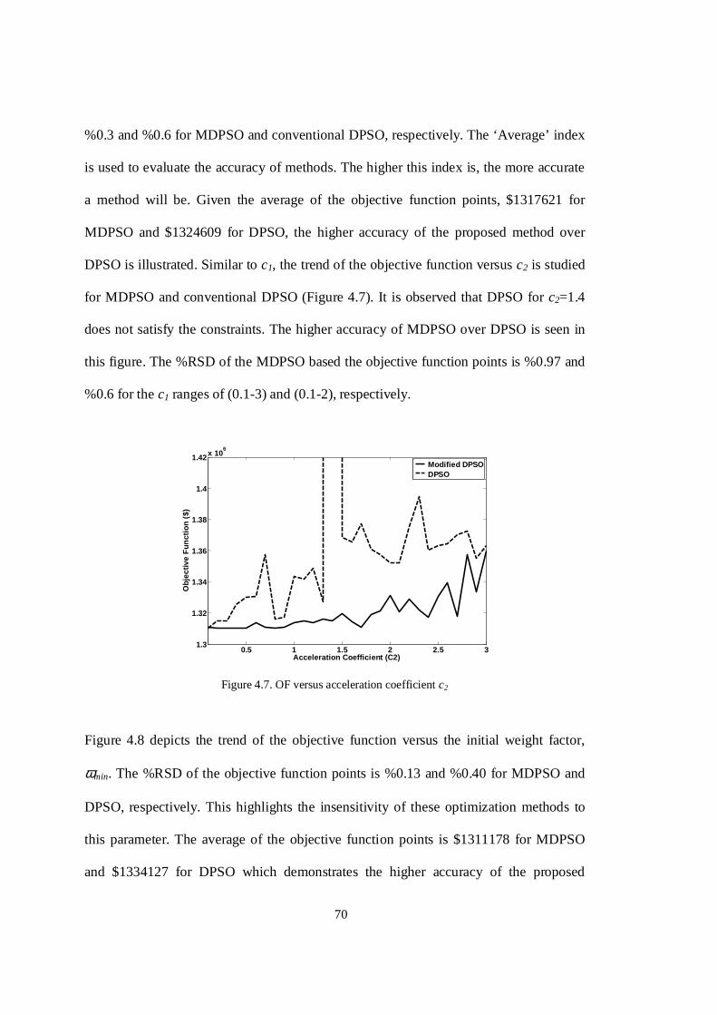
70
%0.3 and %0.6 for MDPSO and conventional DPSO, respectively. The ‘Average’ index
is used to evaluate the accuracy of methods. The higher this index is, the more accurate
a method will be. Given the average of the objective function points, $1317621 for
MDPSO and $1324609 for DPSO, the higher accuracy of the proposed method over
DPSO is illustrated. Similar to c1, the trend of the objective function versus c2 is studied
for MDPSO and conventional DPSO (Figure 4.7). It is observed that DPSO for c2=1.4
does not satisfy the constraints. The higher accuracy of MDPSO over DPSO is seen in
this figure. The %RSD of the MDPSO based the objective function points is %0.97 and
%0.6 for the c1 ranges of (0.1-3) and (0.1-2), respectively.
Figure 4.7. OF versus acceleration coefficient c2
Figure 4.8 depicts the trend of the objective function versus the initial weight factor,
ωmin. The %RSD of the objective function points is %0.13 and %0.40 for MDPSO and
DPSO, respectively. This highlights the insensitivity of these optimization methods to
this parameter. The average of the objective function points is $1311178 for MDPSO
and $1334127 for DPSO which demonstrates the higher accuracy of the proposed
0.5 1 1.5 2 2.5 31.3
1.32
1.34
1.36
1.38
1.4
1.42x 10⁶
Acceleration Coefficient (C2)
Ob
ject
ive
Fu
nct
ion
($)
Modified DPSO DPSO

71
technique. A range of (0.1-1) is appropriate for both of the methods because in which,
the objective function variation is negligible.
Figure 4.8. OF versus initial weight factor minω
Similar to this procedure is performed for the final weight factor, ωmax, and ranges of
(0.4-1) and (0.6-1) are selected as the robustness range of this parameter for MDPSO
and DPSO, respectively. In these ranges, %RSD for MDPSO is %0.65 and in
conventional DPSO is %0.85. Furthermore, the average objective function for MDPSO
and conventional DPSO is $1312175 and 1331140, respectively. This shows $18965
cost benefit by employing the proposed method.
As comprehended, both of the MDPSO and DPSO methods are insensitive to a wide
range of their parameters. This robustness verifies the selection of these PSO-based
algorithms as good options for solving the ASC problem. Particularly compared with
DPSO, MDPSO is more robust and accurate.
After studying the robustness, with respect to changes of the PSO parameters, the
robustness with respect to changes of the initial values is investigated. For this purpose,
0.1 0.2 0.3 0.4 0.5 0.6 0.7 0.8 0.9 11.305
1.31
1.315
1.32
1.325
1.33
1.335
1.34
1.345
x 106
Initial Inertia Weight Factor
Ob
ject
ive
Fu
nct
ion
($)
Modified DPSO DPSO

72
the MDPSO, DPSO, GA, and SA are run 25 times and the outputs are sorted by
optimized Objective function value in Figure 4.9.
As observed in Figure 4.9, the robustness of MDPSO is more than others (%RSD by
MDPSO is %0.138 being lower than %0.766 by DPSO, %0.953 by GA, and %4.01 by
SA). Higher robustness and accuracy features highlight the priority of MDPSO over the
other methods for capacitor planning.
Figure 4.9. A comparison of objective functions
Table 4.1 shows a summary of the results. As observed in Table 4.1, MDPSO is the
most accurate method compared with DPSO, GA and SA for capacitor planning in this
case study (the error of average from the best point which is 1.3102×10⁶ by MDPSO is
$1500 by DPSO is $13300, by GA is $22900, and by SA is $57600). This means
$11800, $21400, and $56100 cost benefits are gained by employing MDPSO instead of
DPSO, GA and SA, respectively. A comparison among the MDPSO, DPSO, GA, and
SA along with the total cost with no installed capacitor is given in Table 4.2. In these
5 10 15 20 251.3
1.35
1.4
1.45
1.5
x 106
Run Number
Ob
ject
ive
Fu
nct
ion
($)
Modified DPSO DPSO GA SA

73
heuristic methods, the median solution among the 25 runs is selected as the average
value and is given in Table 4.2.
Table 4.1. Comparison of optimization methods
Worst ($) Best ($) Average
Error ($) %RSD
SA 1.5049×10⁶ 1.33231×10⁶ 57600 4.010
GA 1.3795×10⁶ 1.3147×10⁶ 22900 0.953
DPSO 1.3488×10⁶ 1.3122×10⁶ 13300 0.766
MDPSO 1.3153×10⁶ 1.3102×10⁶ 1500 0.138
Table 4.2. Comparison of MDPSO, DPSO, GA, SA, and ‘No Capacitor’ state
Capacitors Size
(kvar)
Capacitor
Cost ($)
Loss
(kW)
Loss Cost
($)
Total Cost
$
No Capacitor 0 0 332.1 1.849×10⁶ 1.849×10⁶
SA 8100 6.243×10⁴ 234.4 1.3054×10⁶ 1.3678×10⁶
GA 7800 6.012×10⁴ 229.4 1.2774×10⁶ 1.3375×10⁶
DPSO 7800 6.012×10⁴ 227.3 1.2658×10⁶ 1.3259×10⁶
MDPSO 7500 5.781×10⁴ 225.2 1.2540×10⁶ 1.3118×10⁶
Table 4.2 illustrates that the total cost decreases from $1849000 to $1311800 by
installing the capacitors ($537200 cost benefit). This underlines the importance of
allocation and sizing of capacitors in a distribution system for minimizing the line loss.
DNLP was also applied for capacitor planning, but it could not move from the initial
values for many random initial values. This shows the objective function has several
local minima. Compared with other heuristic methods, MDPSO is demonstrated to be

74
more accurate and robust for this case. The trend of the objective function is depicted in
Figure 4.10 for the iteration number after 8. It should be noted that the objective
function includes high penalty factors due to constraint violation in the first 8 iterations.
Figure 4.11 shows a comparison between the voltage profile before and after the
installation of capacitors.
Figure 4.10. Trend of OF versus iteration number
Figure 4.11. Voltage profile before and after installation of capacitors
20 40 60 80 100 120 140 160 180 2001.3
1.35
1.4
1.45x 10⁶
Iteration Number
Ob
jec
tive
Fu
nct
ion
($
)
1 2 3 4 5 6 7 8 9 20 21 22 23 24 25 260.91
0.92
0.93
0.94
0.95
0.96
0.97
0.98
0.99
1
Bus Number
Bu
s V
olt
age
(PU
)
Before Installation After Installation
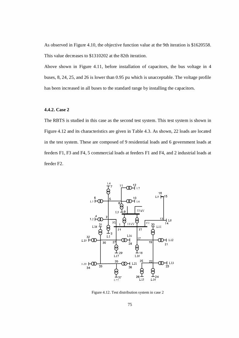
75
As observed in Figure 4.10, the objective function value at the 9th iteration is $1620558.
This value decreases to $1310202 at the 82th iteration.
Above shown in Figure 4.11, before installation of capacitors, the bus voltage in 4
buses, 8, 24, 25, and 26 is lower than 0.95 pu which is unacceptable. The voltage profile
has been increased in all buses to the standard range by installing the capacitors.
4.4.2. Case 2
The RBTS is studied in this case as the second test system. This test system is shown in
Figure 4.12 and its characteristics are given in Table 4.3. As shown, 22 loads are located
in the test system. These are composed of 9 residential loads and 6 government loads at
feeders F1, F3 and F4, 5 commercial loads at feeders F1 and F4, and 2 industrial loads at
feeder F2.
Figure 4.12. Test distribution system in case 2
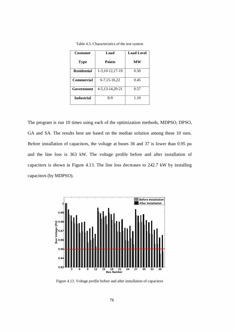
76
Table 4.3. Characteristics of the test system
Customer
Type
Load
Points
Load Level
MW
Residential 1-3,10-12,17-19 0.50
Commercial 6-7,15-16,22 0.45
Government 4-5,13-14,20-21 0.57
Industrial 8-9 1.10
The program is run 10 times using each of the optimization methods, MDPSO, DPSO,
GA and SA. The results here are based on the median solution among these 10 runs.
Before installation of capacitors, the voltage at buses 36 and 37 is lower than 0.95 pu
and the line loss is 363 kW. The voltage profile before and after installation of
capacitors is shown in Figure 4.13. The line loss decreases to 242.7 kW by installing
capacitors (by MDPSO).
Figure 4.13. Voltage profile before and after installation of capacitors
3 6 9 12 15 18 21 24 27 30 33 360.93
0.94
0.95
0.96
0.97
0.98
0.99
1
Bus Number
Bu
s V
olt
age
(PU
)
Before Installation After Installation

77
As shown in Figure 4.13, the bus voltage at all buses has been increased to more than
0.95 pu by installing the capacitors. In order to evaluate the proposed method, the results
are compared with DPSO, GA, SA, and ‘No Capacitor’ state (Table 4.4).
Table 4.4. Comparison of MDPSO, DPSO, GA, SA, and ‘No Capacitor’ state
Capacitors Size
(kvar)
Capacitor
Cost ($)
Loss
kW
Loss Cost
($)
Total Cost
($)
No
Capacitor 0 0 363 2.0212×10⁶ 2.0212×10⁶
SA 7500 5.781×10⁴ 267.7 1.4906×10⁶ 1.5484×10⁶
GA 8400 6.475×10⁴ 247.6 1.3785×10⁶ 1.4432×10⁶
DPSO 7500 5.781×10⁴ 277.5 1.5451×10⁶ 1.6029×10⁶
MDPSO 8100 6.243×10⁴ 242.7 1.3514×10⁶ 1.4138×10⁶
As shown in Table 4.4, the MDPSO demonstrates higher accuracy rather than DPSO,
GA, and SA, the average total cost by MDPSO is $1413800, by DPSO is $1602900, by
GA is $1443200, and by SA is $1548400. As mentioned, the analytical methods (e. g.
DNLP) do not deal appropriately with the problem with several local minima. This is
revealed in this case similar to case 1, the DNLP cannot move from its initial values for
many random initial values.
Similar to case 1, the importance of allocation and sizing of capacitors for minimizing
the line loss is approved in this case so that the total cost decrease from $2021200 to
$1413800 by installing the capacitors. The reasonable accuracy and robustness of the
proposed MDPSO lead this method as a good choice for the capacitors planning
problem.

78
If the required reactive power of all buses is provided by a capacitor located at the
corresponding bus, the line loss is decreased to 239 kW. This reveals that the loss cannot
be decreased to lower than 239 kW only by using capacitors; since, the rest of line loss
is related to the active power.
4.5. Summary
In this chapter, the MDPSO method is presented to optimize the location and size of
capacitors in a distribution system to minimize the line loss. The objective function is
composed of the capacitors investment cost and the line loss which is converted into the
genuine dollar. The bus voltage and the feeder current as constraints are maintained
within the standard level.
Given the discrete nature of the capacitors planning problem, selection of a proper
optimization method is important. The heuristic based methods deal appropriately with
the local minima. Among these methods, DPSO is employed in this chapter. To increase
the diversity of the variables, DPSO is developed by the crossover and mutation
operators.
The proposed method is evaluated by two test systems, the 18-bus IEEE test system and
the modified semi-urban distribution system connected to bus 2 of the RBTS. The
robustness and accuracy of the method is studied with respect to changes of the
parameters and changes of the initial values. The results are compared with ‘No
Capacitor’ state, DNLP as an analytical method, and three heuristic methods, DPSO,
GA and SA. It is revealed that a high cost benefit is found by installing the capacitors.
DNLP could not move from its initial values for many random choices of initial values.

79
Compared with DPSO, GA and SA, MDPSO presents lower %RSD and average
objective function which illustrates its higher robustness and accuracy for planning the
capacitors.

80

81
CHAPTER 5
Distribution System Planning for Minimizing Line
Loss and Improving Voltage Profile
5.1. Introduction
As mentioned before, the line loss and voltage profile are two main concerns in planning
distribution networks. These two can be improved by employing capacitors and VRs
and by adjusting the operation of LTCs and VRs.
In this chapter, the operation of VRs, capacitors, HV/MV transformer tap changers
along with the location of VRs and capacitors are determined for minimizing the line
loss and improving the voltage profile when the load level is time varying. For this
purpose, the MDPSO proposed in the previous chapter is employed. It should be noted
that direct optimization of the tap position is not appropriate since in general the HV
side voltage is not known. Therefore, the tap setting can be determined given the
Voltage on Customer side of Transformer (VCT) once the HV side voltage is known.
The objective function for the optimization is composed of the distribution line loss cost,
the peak power loss cost and capacitors’ and VRs’ capital, operation and maintenance
costs. The constraints on the optimization program are composed of the bus voltage and
feeder current along with VR taps. The bus voltage should be maintained within the
standard level and the feeder current should not exceed the feeder rated current. The taps
are to adjust the output voltage of VRs between 90% and 110% of their input voltages.
82
For validation of the proposed method, the 18-bus IEEE system is used. The results are
compared with prior publications to illustrate the benefit of the employed technique. The
results also show that the lowest cost planning for voltage profile will be achieved if a
combination of capacitors, VRs and VCTs is considered.
5.2. Problem Formulation
The main objective of the Planning of Capacitors and VRs and the optimization of VCT
(PCVV) problem is to minimize the cost of capacitors and VRs as well as the
distribution line loss and peak power which will require higher investment of using high
rating equipment. This is achieved by reducing the power loss at the peak load. The bus
voltage and the feeder current are also limited as constraints and added to the objective
function with a penalty factor. The bus voltage is maintained within the standard range.
The feeder current should be kept lower than the rated current of the relative feeder. The
tap setting of VRs is adjusted during the optimization procedure to minimize the line
loss and improve the voltage profile. The taps are practically limited to ±10%.
Given that all of the objective function elements are simply converted into the
composite equivalent cost, this problem can be solved using a single-objective
optimization method. This objective is defined as (3.1) in which CI is zero. The capital
cost is composed of the cost for installing and purchasing the capacitors and VRs. The
operation and maintenance costs are self explanatory. The loss cost is expressed in (5.1).
As observed, the loss cost has two parts, the energy loss cost which is proportional to the
cost per MWh and the peak power cost which is proportional to the cost saving per MW
reduction in the peak power.

83
CL = kPL× LLLossP + kL× ∑=
LL
1llLossll ll
P.T (5.1)
where LL is the number of load levels and Tll is the duration of load level ll . The
constraints include the bus voltage and the feeder current. The bus voltage should be
maintained within the standard level as (3.6) and (3.7). Additionally, tap setting as a
constraint should be limited to ±10%. At any load level, when a switched capacitor bank
is connected or disconnected, the bus voltage increases or decreases, respectively. To
minimize the effect on customers, this voltage change is limited to a value in the range
of 2% to 3%. A good approximation to the voltage change is given in [124].
%100MVA
QV
SC
C ×
=∆ (5.2)
Here V∆ is the voltage change (assumed 3% in this chapter), QC is the size of a switched
capacitor bank, and MVASC is the available three-phase short-circuit MVA at the bus,
where the capacitor bank is located. Given this equation, the maximum permitted size of
a switched capacitor bank can be determined.
5.3. Methodology
The methods presented for scheduling of VRs either find only VRs location and tap
setting [52,53], or treat VRs separately from capacitors [125-127]. Using these
approaches, solving the problem for a specific load level will not lead to accurate results
when the load level is time varying.
The papers that deal with capacitor either focus on the scheduling of capacitors and
LTCs [62-64], or concentrate on the allocation and sizing of only capacitors [54-61].
These papers are generally follow one of the following strategies:

84
1. The capacitors are allocated and sized for the lowest load level as the fixed capacitors.
Subsequently, the problem is solved for higher load levels and the additional capacitors
are presumed as the switched capacitors [55-57] (Building Strategy).
2. The capacitors are obtained in all load levels; then, the minimum capacitor in each
bus is assumed as the fixed capacitor and the rest as the switched capacitors [59-61]
(Separating Strategy).
3. All of the load levels are optimized simultaneously. The optimization method should
solve a problem with (number of buses × number of load level) optimization variables
[128].
In the first strategy, the capacitors obtained for higher load levels are not used for lower
load levels while they can be used for loss minimization and voltage profile
improvement with applying no extra cost. In addition to the shortcoming mentioned for
the first strategy, the second strategy suffers from having a large number of buses for
installation of capacitors, which implies a high installation cost because there is no
guarantee that the placement for a capacitor in a load level is determined the same in
next load level. Eventually, in the techniques associated with the third strategy, the
number of variables severely increases the computation time and decreases the accuracy.
The aforementioned limitations highlight the necessity of an appropriate technique to
incorporate the influence of LTCs, VRs and capacitors simultaneously and to include
the multi-load level assumption. There is also a need to have a compromise between the
accuracy and computation time.
As mentioned, increasing the number of variables leads to a more complex optimization
problem and so lower accuracy. For alleviating this problem, using a segmentation-
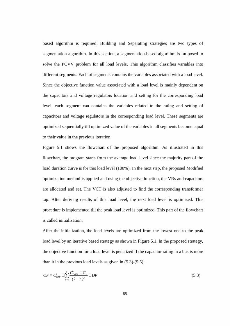
85
based algorithm is required. Building and Separating strategies are two types of
segmentation algorithm. In this section, a segmentation-based algorithm is proposed to
solve the PCVV problem for all load levels. This algorithm classifies variables into
different segments. Each of segments contains the variables associated with a load level.
Since the objective function value associated with a load level is mainly dependent on
the capacitors and voltage regulators location and setting for the corresponding load
level, each segment can contains the variables related to the rating and setting of
capacitors and voltage regulators in the corresponding load level. These segments are
optimized sequentially till optimized value of the variables in all segments become equal
to their value in the previous iteration.
Figure 5.1 shows the flowchart of the proposed algorithm. As illustrated in this
flowchart, the program starts from the average load level since the majority part of the
load duration curve is for this load level (100%). In the next step, the proposed Modified
optimization method is applied and using the objective function, the VRs and capacitors
are allocated and set. The VCT is also adjusted to find the corresponding transformer
tap. After deriving results of this load level, the next load level is optimized. This
procedure is implemented till the peak load level is optimized. This part of the flowchart
is called initialization.
After the initialization, the load levels are optimized from the lowest one to the peak
load level by an iterative based strategy as shown in Figure 5.1. In the proposed strategy,
the objective function for a load level is penalized if the capacitor rating in a bus is more
than it in the previous load levels as given in (5.3)-(5.5):
DP)r1(
CCCOF
Y
1yy
LM&OCAP +
++′
+′= ∑=
(5.3)

86
−
=′−
jbusatiscapacitornoifC
jbusatiscapacitoraifCCC
llCAP
1llCAP
llCAP
jCAP
j
jj (5.4)
=
>−
≤<
=′−
−−
−
0CifC
CCifCC
CC0if0
C
1llll
1llll1llll
1llll
M&O
M&OjM&O
M&OM&OjM&OjM&O
M&OM&O
j (5.5)
where llCAPj
C and ll
jM&OC are the capital cost and the operation and maintenance cost of a
device at bus j for load level ll , respectively.
Figure 5.1. Flowchart of the proposed algorithm

87
Adding a capacitor at a bus where another capacitor has been already installed causes a
back-to-back switching problem [124]. One of the solutions of this problem is to add a
current limiting reactor [124]. Therefore, two different types of switched capacitors are
used in this method, switched capacitors with reactor and without reactor. The
installation cost of a switched capacitor with reactor is more than the cost of one without
reactor. During the optimization procedure, if a single capacitor bank is installed at a
bus, it does not need a reactor. Any further switched capacitor at that bus will need to
include the cost of a reactor.
The proposed procedure increases the probability of selecting the optimized locations in
the previous load level as the locations in the current load level. While, it does not force
the program to select the devices found for the previous load level as the fixed devices
for the current load level. This leads the program to results with lower investment cost
and line loss.
After the completion of an iteration from the lowest to the highest load level, the
minimum capacitor size in a bus in the iteration is considered as the fixed capacitor and
the rest as the switched capacitor installed. The tap setting of VRs and the VCTs in each
load level are also optimized during this procedure.
5.4. Applying Modified DPSO to PCVV
This problem is solved using the proposed MDPSO, which was described in the
previous chapter (Figure 4.2). The PSO parameters selected for the algorithm are as
follows: population size = 400, iteration number = 1000, acceleration coefficients c1 = c2
= 0.5 and inertia weight factor ω = 0.9. The GA parameters, mutation and crossover
88
rates, are selected as 0.2 and 0.5. The acceleration coefficients, inertia weight factors,
and the mutation and crossover rates are kept fixed for all uses of MDPSO in the next
chapters.
The first stage in the optimizing procedure is to determine the variables, which are the
discrete capacitors size as well as the VR and the VCT. It is assumed that all buses are
candidate for installation of VRs and capacitors. Given these points, the particle is
constituted as shown in Figure 5.2.
Figure 5.2. The structure of a particle
In Figure 5.2, NB and NT are the number of buses and VCTs in the optimizing
distribution system. Each member of this particle is assigned as a placement of a device.
The value of the corresponding member is the size of capacitors, the tap setting of VRs,
and VCTs. For the capacitors, if the value of this member is more than a specific
threshold, it indicates a capacitor with the corresponding size installed at the
corresponding bus. Otherwise, no capacitor is placed at that bus. This specific threshold
is the minimum size of the available set of capacitors. For the VRs, the member value is
the tap setting. If the tap setting is equal to 1, no VR is installed at the corresponding
bus. Otherwise, a VR with the corresponding tap setting is installed at the corresponding

89
bus. The same procedure as VRs is implemented for optimizing the tap setting of
transformers.
5.5. Results
To validate the proposed method, the 12.5 kV 18-bus IEEE distribution system
[19,100,123] is used (Figure 4.5) with parameters given in Table 5.1 to provide practical
current limits and realistic conductor impedances.
Table 5.1. Test system line data and conductors data
Lines Conductor Type R
(Ω)
X
(Ω)
Current Rating
(A)
1-2 1 0.0816 0.207 724
2-3,3-4,4-5 2 0.0995 0.212 648
1-20,20-21 3 0.167 0.228 441
5-6,6-7,21-23 4 0.367 0.256 259
7-8,2-9,21-22,
23-24,23-25,25-26 5 1.31 0.296 108
The load duration curve of this test system is shown in Figure 5.3. The most complex
but accurate way is to study the network and solve the PCVV problem for every point in
this curve. However, this procedure is excessively time consuming. On the other hand,
the easiest and fastest but least accurate way is to approximate the load duration curve
with 2-3 levels (as implemented in most papers) and solve the PCVV problem based on
small number load levels.

90
Figure 5.3. Load duration curve used in the testing distribution system
In this chapter, to implement a compromise between accuracy and computation time,
this curve is approximated with 5 load levels. It is assumed that the load peaks for 2% of
the time and is at its lowest for 3% of the time. The average load is drawn from the
network for 40% of the time. For 30% and 25% of the time, the load level is 120% and
80% of the average load, respectively. However, using sensitivity analysis to find the
load level number can be included in the future.
It is assumed that the cost per kWh is different for different load levels, 3 ¢ for 50% and
80% of the average load, 6 ¢ for 100%, 8 ¢ for 120% and 10 ¢ for peak load level. These
prices are in the same range of [129-131] and show a similar trend to the generating
electricity cost from different types of technology in the UK [132]. The saving per MW
reduction in the peak power loss is presumed to be $168000. The installation cost of
switched capacitors with reactor and without reactor is assumed to be $(3000+45/kvar)
and $(3000+25/kvar), respectively. The annual incremental cost is supposed to be
1$/kvar. Application of constraint (5.2) for this test system results in a capacitor bank
91
step of 150kvar. For the VRs, the installation cost is presumed $10000 and the annual
incremental cost is selected as $300. The VRs are characterized by 32 taps which can
change the output voltage between 0.9 and 1.1 times of the input voltage. Therefore,
each step can change the input voltage as 0.00625 pu. The coding is written in Matlab
7.6 programming language and is executed in a desktop computer with the features as
Core 2 Due CPU, 2.66 GHz, and 2 GB of RAM.
Adding current limiting reactors or pre-insertion resistors increases the cost of
capacitors. This penalty decreases the number and size of capacitors significantly. This
decrease in size will alleviate the problem of nuisance tripping and voltage
magnification of modern load sensitive to electromagnetic transients. For particular
sensitive busses, solutions such as point-on-wave switching [133] will give rise to an
additional cost for capacitor banks in the optimization.
When no capacitor is installed, the minimum and maximum line losses related to the
lowest and highest load levels are 87.3 kW and 801.6 kW respectively. The standard
range of the bus voltage is assumed to be between 0.95 pu and 1.05 pu. Given this, the
bus voltage constraint for the lowest load level is satisfied, but for the peak load, the bus
voltage at 8 buses violates the voltage constraint. In order to decrease the line losses and
to improve the voltage profile, VRs and capacitors are allocated and the capacitors size
as well as the VR and the LTC taps are adjusted.
To clarify the importance of consideration of both capacitors and VRs in the line loss
minimization and bus voltage improvement, three cases are studied. In the first case, the
objective function is only composed of the capacitors. Only VRs are included in the
objective function in the second case. Finally, both of VRs and capacitors are involved

92
in the objective function in the third case. In all of these cases, the VCT is optimized for
all load levels.
5.5.1. Case 1
In this case only capacitors are used for minimizing the line loss and improving the
voltage profile. The capacitor locations and ratings as well as the optimization of VCT
for different load levels are shown in Table 5.2. As observed in this table, 3 fixed
capacitors are required to minimize the line loss in the test system. The scheduling of the
switched capacitors is given in Table 5.3.
Table 5.2. Capacitors location and rating (Mvar) and VCT
Bus Number
VCT 8 24 25 26
Load
Lev
el
50% 0.60 0.30 0.60 ---- 0.9775
80% 0.60 0.45 0.75 0.15 0.9949
100% 0.60 0.45 0.75 0.45 1.0057
120% 0.60 0.45 0.75 0.60 1.0188
160% 0.60 0.45 0.75 0.60 1.0497
Fixed Capacitor 0.6 0.30 0.60 ----
Table 5.3 illustrates that the switched capacitors should be allocated at 3 buses, 24, 25,
and 26. When the load level is average, 1 bank at bus 24, 1 bank at bus 25, and 3 banks
at bus 26 should be switched on along with the fixed capacitors to result minimum line
loss in this load level.

93
Table 5.3. Scheduling of switched capacitors
Bus Number
8 24 25 26
Load
Lev
el
50% ---- ---- ---- ----
80% ---- 0.15 0.15 0.15
100% ---- 0.15 0.15 0.45
120% ---- 0.15 0.15 0.60
160% ---- 0.15 0.15 0.60
Switched Capacitor ---- 0.15 0.15 0.60
Figures 5.4 and 5.5 show the line loss and the voltage profile after and before
installation of the capacitors. A remarkable reduction is observed in the line loss for all
load levels. Furthermore, the bus voltage constraint in the peak load level is satisfied
when the capacitors are allocated optimally. It should be noted that the line loss before
the installation of capacitors is based on the assumption that the VCT is equal to 1 pu. It
should also be noted that the line losses before installation of capacitors for the 100%,
120% and peak load level cases are invalid because the voltage constraint is not
satisfied. However, these are shown in Figure 5.4 only to illustrate the effect of
capacitors. The calculations show that increasing the VCT (or LTC tap setting) results in
more line loss when no capacitor is installed. For example, when the load level is 120%,
the line loss is 469 kW. As observed in Table 5.2, the VCT is adjusted to 1.0188 pu for
this load level to have an acceptable bus voltage. In this condition, the line loss increases
to 481 kW. Therefore, the capacitors are partly used for improving the voltage profile,
partly for compensating the line loss increase due to the increment of the VCT (LTC tap
setting) and also partly for minimizing the loss.

94
Figure 5.4. Line loss before and after installation of capacitors
Figure 5.5. Voltage profile before and after installation of capacitors in peak load (Case 1 (CAP))
To validate the proposed strategy, the results are compared with the strategies
mentioned in section 5.3, (Building and Separating Strategies). Table 5.4 shows the
results obtained using these strategies.
1 2 3 4 50
100
200
300
400
500
600
700
800
900
Load Level
Lin
e L
oss
(kW
)
Before Installation After Installation
1 2 3 4 5 6 7 8 9 20 21 22 23 24 25 260.86
0.88
0.9
0.92
0.94
0.96
0.98
1
1.02
1.04
Bus Number
Bu
s V
olt
age
(pu
)
Before Installation After Installation

95
Table 5.4. Scheduling of switched capacitors
Bus Number
8 23 24 25 26
Building
Strategy
Fixed Capacitor ---- ---- ---- ---- ----
Switched Capacitor 0.75 ---- 0.45 0.75 0.60
Separating
Strategy
Fixed Capacitor ---- ---- ---- ---- ----
Switched Capacitor 0.75 0.15 0.15 1.05 1.20
These strategies start from the lowest load level. Therefore, when no capacitor is found
for this load level in the test system, no fixed capacitor is found by these strategies. The
corresponding results are evaluated in sub-section 5.5.3.
The allocation and sizing of capacitors along with scheduling of switched capacitors and
optimization of VCT was studied in case 1. In addition to the capacitors and the VCT,
the VRs are other devices which influence the line loss and the voltage profile.
5.5.2. Case 2
Case 2 investigates VRs and their placement and scheduling for minimizing the line loss
and improving the voltage profile. The scheduling of VRs and VCT (LTC) is shown in
Table 5.5.
Figure 5.6 shows the voltage profile before and after installation of VRs. Improvement
of the voltage profile is observed after installation of VRs. The main difference between
capacitors and VRs is that capacitors inject the reactive power to the distribution
network and reduce the reactive-element of the line loss. But, VRs do not have this
influential characteristic.
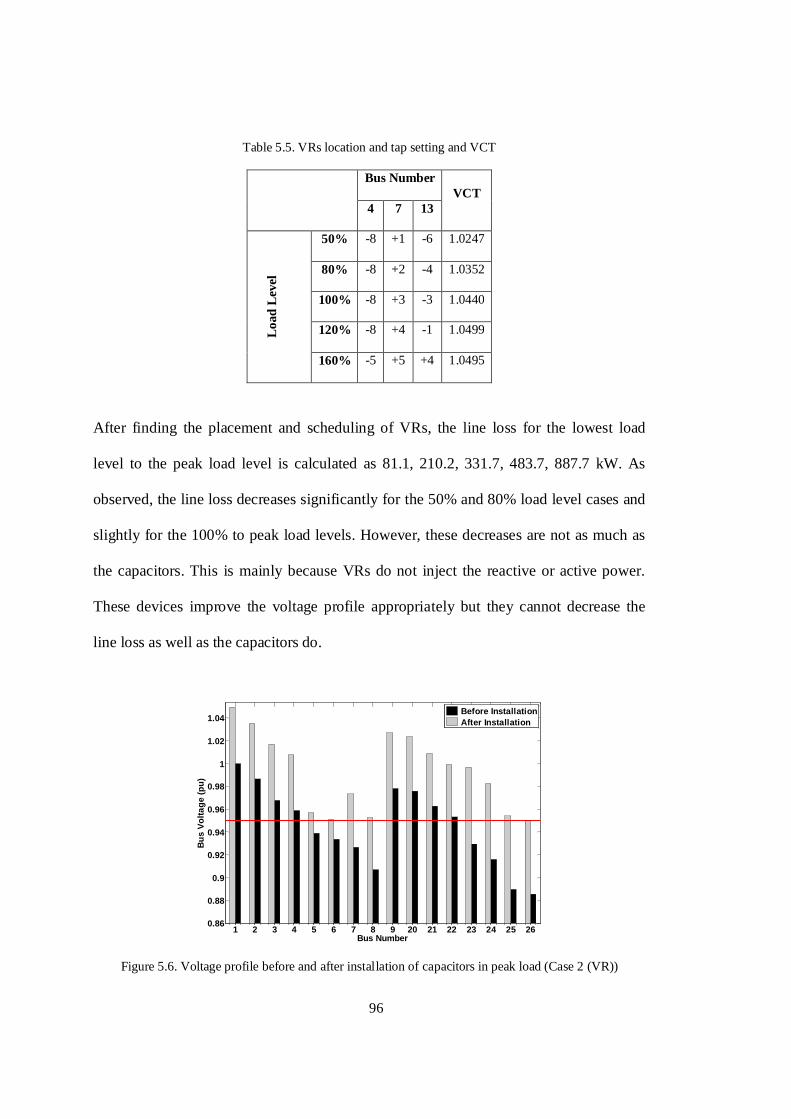
96
Table 5.5. VRs location and tap setting and VCT
Bus Number
VCT 4 7 13
Load
Lev
el
50% -8 +1 -6 1.0247
80% -8 +2 -4 1.0352
100% -8 +3 -3 1.0440
120% -8 +4 -1 1.0499
160% -5 +5 +4 1.0495
After finding the placement and scheduling of VRs, the line loss for the lowest load
level to the peak load level is calculated as 81.1, 210.2, 331.7, 483.7, 887.7 kW. As
observed, the line loss decreases significantly for the 50% and 80% load level cases and
slightly for the 100% to peak load levels. However, these decreases are not as much as
the capacitors. This is mainly because VRs do not inject the reactive or active power.
These devices improve the voltage profile appropriately but they cannot decrease the
line loss as well as the capacitors do.
Figure 5.6. Voltage profile before and after installation of capacitors in peak load (Case 2 (VR))
1 2 3 4 5 6 7 8 9 20 21 22 23 24 25 260.86
0.88
0.9
0.92
0.94
0.96
0.98
1
1.02
1.04
Bus Number
Bu
s V
olt
age
(pu
)
Before Installation After Installation
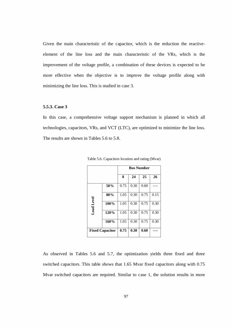
97
Given the main characteristic of the capacitor, which is the reduction the reactive-
element of the line loss and the main characteristic of the VRs, which is the
improvement of the voltage profile, a combination of these devices is expected to be
more effective when the objective is to improve the voltage profile along with
minimizing the line loss. This is studied in case 3.
5.5.3. Case 3
In this case, a comprehensive voltage support mechanism is planned in which all
technologies, capacitors, VRs, and VCT (LTC), are optimized to minimize the line loss.
The results are shown in Tables 5.6 to 5.8.
Table 5.6. Capacitors location and rating (Mvar)
Bus Number
8 24 25 26
Load
Lev
el
50% 0.75 0.30 0.60 ----
80% 1.05 0.30 0.75 0.15
100% 1.05 0.30 0.75 0.30
120% 1.05 0.30 0.75 0.30
160% 1.05 0.30 0.75 0.30
Fixed Capacitor 0.75 0.30 0.60 ----
As observed in Tables 5.6 and 5.7, the optimization yields three fixed and three
switched capacitors. This table shows that 1.65 Mvar fixed capacitors along with 0.75
Mvar switched capacitors are required. Similar to case 1, the solution results in more
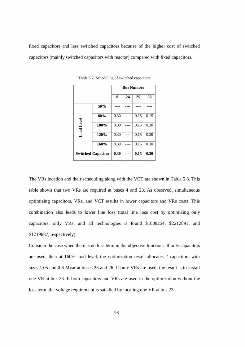
98
fixed capacitors and less switched capacitors because of the higher cost of switched
capacitors (mainly switched capacitors with reactor) compared with fixed capacitors.
Table 5.7. Scheduling of switched capacitors
Bus Number
8 24 25 26
Load
Lev
el
50% ---- ---- ---- ----
80% 0.30 ---- 0.15 0.15
100% 0.30 ---- 0.15 0.30
120% 0.30 ---- 0.15 0.30
160% 0.30 ---- 0.15 0.30
Switched Capacitor 0.30 ---- 0.15 0.30
The VRs location and their scheduling along with the VCT are shown in Table 5.8. This
table shows that two VRs are required at buses 4 and 23. As observed, simultaneous
optimizing capacitors, VRs, and VCT results in lower capacitors and VRs costs. This
combination also leads to lower line loss (total line loss cost by optimizing only
capacitors, only VRs, and all technologies is found $1808254, $2212891, and
$1719887, respectively).
Consider the case when there is no loss term in the objective function. If only capacitors
are used, then at 160% load level, the optimization result allocates 2 capacitors with
sizes 1.05 and 0.6 Mvar at buses 25 and 26. If only VRs are used, the result is to install
one VR at bus 23. If both capacitors and VRs are used in the optimization without the
loss term, the voltage requirement is satisfied by locating one VR at bus 23.

99
Table 5.8. VRs location and tap setting and VCT
Bus
Number VCT
4 23
Load
Lev
el
50% -8 -7 1.0224
80% -8 -7 1.0398
100% -8 -7 1.0499
120% -6 -4 1.0491
160% -2 +1 1.0495
The dominance of loss control by capacitors is supported by the results in Table 5.9
where the capacitors only (case 1) results in much lower line loss compared with VRs
(case 2). These points illustrate that for the cost levels in this method, the main role of
VRs is for voltage control while capacitors are mainly used to reduce the line loss. That
is why the placement of capacitors and VRs do not necessarily change when they are
combined in case 3.
Associated with the load level changes from 100%, 120% to 160%, the corresponding
load durations are from 40%, 25% to 3%. There is a substantial increase in the loss at
160% but because the duration is low, there is insufficient justification for a change in
capacitor size. Tables 5.6 and 5.7 show no change of capacitor size was obtained when
the VRs are available. In case 1, the capacitors have two roles, voltage control and loss
minimization. Because the voltage control is a compulsory requirement then an increase
of capacitors with loading levels is seen.
If VRs type is the Automatic Voltage Regulators (AVRs), the output voltage set point
can be found using the voltage obtained when the tap setting, given in Table 5.8, is

100
applied to the VRs in each load level. For example, when the network is supplying the
peak load level, the VRs tap is set to -2 and +1, respectively. This setting leads their
output voltage to be 0.9975 and 0.9916 pu for the VRs located at buses 4, and 23,
respectively. Therefore, to minimize the line loss along with improving the voltage
profile, these values can be selected as their voltage set point when their type is AVR
and their tap cannot be set manually.
Figure 5.7 reveals the voltage profile for the peak load obtained after the allocation and
sizing of capacitors along with the allocation and scheduling of VRs and optimization
the VCT. The line loss in this case is decreased to 60.82, 157.76, 252, 376.44, and
727.44 kW for the load levels respectively.
Figure 5.7. Voltage profile before and after installation of capacitors in peak load (Case 3 (CAP&VR))
A comparison among the above cases is given in Table 5.9. In Table 5.9, the line losses
for the 100%, 120%, and peak load levels related to the ‘No Installation’ are in brackets
to show that the voltage constraint is not satisfied in these load levels so the results are
1 2 3 4 5 6 7 8 9 20 21 22 23 24 25 260.86
0.88
0.9
0.92
0.94
0.96
0.98
1
1.02
1.04
Bus Number
Bu
s V
olt
age
(pu
)
Before Installation After Installation

101
invalid. As observed in this table, compared with ‘No Installation’ case, the proposed
strategy enjoys $326327 less total cost. The total cost calculated by the proposed
strategy is $68012 less than it when only the capacitors are allocated and sized. This
remarkable difference shows the importance of the consideration of VRs and LTC tap
setting along with the capacitors in loss minimization and voltage profile improvement.
Furthermore, compared with the Building and Separating strategies, the proposed
strategy is at least 6.5% ($121928) more cost beneficial.
Table 5.9. A comparison among the cases ($)
Loss Cost for Load Levels Capacitor
Cost
VR
Cost
Total
Cost 50% 80% 100% 120% 160%
No
Installation 4861 181082 (739585) (870128) (357839) 0 0 (2153495)
Case 1
(CAP) 3544 140330 599010 735011 330359 86926 0 1895180
Case 2
(VR) 4516 175600 738758 897740 396277 0 39535 2252426
Case 3
(CAP&VR) 3386 131764 561296 698704 324737 80925 26356 1827168
Building
Strategy 4742 177684 619097 734476 327344 153765 0 2017108
Separating
Strategy 4742 177684 619097 744224 352999 177460 0 2076206

102
5.6. Summary
A comprehensive study is performed for minimizing the line loss and improving the
voltage profile in this chapter. In this study, almost all distribution system devices which
influence the voltage profile, e.g. capacitors, VRs, and LTC, are incorporated.
Optimization of the LTC tap setting is not meaningful since the HV side voltage is not
known. Therefore, the VCT is optimized in this chapter. The LTC tap setting can be
determined given the VCT once the HV side voltage is known.
Planning for all load levels in practical networks results in dealing with a large number
of variables. To handle this problem, a segmentation-based strategy is proposed in this
chapter. This technique classifies the variables associated with a load level in a segment
and solves them in their own segment. Finally, an algorithm is used to solve these
segments sequentially for finding variables associated with whole system. Given the
discrete nature of the problem and the devices rating, the local minima are the main
issue of this optimization procedure. Therefore, a PSO-based optimization method is
developed by the GA operators to increase the diversity of the variables (MDPSO).
The 18-bus IEEE test system is modified and used for evaluating the proposed strategy.
The results are found in three different categories: the capacitors and VCT, the VRs and
VCT, and the capacitors, VRs and VCT. The results prove the necessity of consideration
of all these devices simultaneously. The results obtained by optimizing only the
capacitors are also compared with some of the available strategies. The results
demonstrate that the proposed strategy has reasonable cost benefit. The results also
illustrate that the lowest cost planning is achieved by combining all the currently
available technologies.

103
CHAPTER 6
Distribution System Planning for Improving Line
Loss, Voltage Profile, and Reliability
6.1. Introduction
In the previous chapter, capacitors and VRs along with the VCTs were included in the
system optimization for minimizing the distribution line loss and for improving the
voltage profile. Although these elements improve line loss and voltage profile
significantly, they do not influence system reliability cost which will be shown to be the
dominant factor in the total cost, particularly for distribution networks located in semi-
urban and rural areas.
To increase system reliability, DGs are allocated and sized in this chapter as part of the
integrated optimization. Since these elements are quite expensive, the capacitors are also
simultaneously planned. Since the cost benefit due to using VRs is not remarkable
(3.6% in Chapter 5), these devices are not included in this chapter.
In this chapter, a comprehensive planning methodology is proposed that can minimize
the line loss, maximize the reliability and improve the voltage profile in a distribution
network. The injected active and reactive power of DGs and the installed capacitor sizes
at different buses and for different load levels are optimally controlled. The tap setting
of HV/MV transformer along with the line and transformer upgrading is also included in

104
the objective function. The MDPSO introduced in Chapter 4 is employed to solve this
nonlinear and discrete optimization problem.
The objective function is composed of the investment cost of DGs, capacitors,
distribution lines and HV/MV transformer, the line loss, and the reliability. All of these
elements are converted into genuine dollars. Given this, a single-objective optimization
method is sufficient. The bus voltage and the line current as constraints are satisfied
during the optimization procedure.
The IEEE 18-bus test system is modified and employed to evaluate the proposed
algorithm. The results illustrate the unavoidable need for control on the DG active and
reactive power and capacitors in distribution networks.
6.2. Problem Formulation
The objective is to minimize the investment cost of DGs, capacitors and distribution
lines, the line loss cost and the reliability cost. The bus voltage and the line current as
constraints are included in the objective function using a constraint penalty factor. The
objective function which is the net present value of the total cost is formulated as
follows:
DPCCCCr
COFY
y
yI
yPL
yL
yMOyCAP ++++
++= ∑
=0& )(
)1(
1 (6.1)
where yM&OC is the total operation and maintenance cost, y
LC is the loss cost, yPLC is the
peak loss cost, and yIC is the reliability cost, all associated with planning interval y. The
discount rate (r) is assumed to be 0.07 in this chapter. The installation cost of DGs and
capacitors are assumed to be proportional to their rating. The operation and maintenance

105
cost of capacitors depends on their rating and the study timeframe. The operation and
maintenance cost of DGs depends on the fuel cost and their working time durations. The
interruption cost (CI) is calculated using (6.2).
∑∑
∑
=
=
=
<
−×+×−
×
≥−××
=LL
1llNL
1l
lll,Lll,DG
l,DG
l,DGlll,L
NS
NL
1l
lll,Lll,DG
lll,LNS
I
PS)DGTRT(S
RT)SP(k
PS)DGTRT(Pk
C (6.2)
where NL is the number of distribution lines, kNS is the customer energy loss penalty
factor ($/MWh), lll,LP is the total power of under outage loads at load level ll when a fault
occurs at line l, SDG,l is the total rating of DGs available to supply the loads under outage
due to a fault at line l, RT is the average time for repairing a line after a fault, and DGT
is the average time for running a DG. The loss cost and the peak loss cost are calculated
using as detailed in equations (6.3) and (6.4).
∑=
××=LL
1llll,LossllLL PTkC (6.3)
CPL = kPL×PLoss,LL (6.4)
where PLoss,ll is the total loss at load level ll and kPL is the cost per MW for supporting
the distribution system at the peak load level.
The constraints are formulated as shown in (3.6) and (3.7) which are referred to the bus
voltage (Vbus) which should be maintained within the standard level and the line current
(I f) which should be less than the line rated current (Ifrated).
In an ideal diesel generator, the fuel consumption is proportional with the load. But in
practice, this relation is not like this and reduced nonlinearly with reducing load so that
even at no load condition, the fuel consumption is roughly between 20% and 40% of the
rated power. Moreover, if the generator operates below a specific rate of the rated power

106
for a long period, serious maintenance problems such as chemical corrosion and glazing
may occur [134, 135].
DGDGllDG SkS .≤ (6.5)
where llDGS is the output power of a DG at load level ll , SDG is the rated power of a DG,
and kDG is to show minimum percentage of the rated power that a DG is allowed to
generate.
6.3. Applying Modified DPSO
The optimization method introduced in Chapter 4 is employed for solving this planning
problem. The population size and iteration number are selected 400 and 1000
respectively. As mentioned before, identifying the variables is the first step in an
optimizing procedure. Figure 6.1 shows the structure of variables in this problem.
Figure 6.1. The structure of a particle
As shown in this figure, the variables are composed of the injected active and reactive
power of DGs at different buses for different load levels, the size of installed capacitors
at different buses for different load levels, the type of distribution lines, and the tap
setting of transformers for different load levels. The HV/MV transformer tap is also set.

107
6.4. Results
To validate the proposed technique, the IEEE 18-bus distribution system [19,100,123] is
used (Figure 4.5). The ideal distribution line in this system is replaced with practical
lines in order to access their rated current. The load duration curve is approximated by
three load levels (160%, 100%, and 50% of the average load) to decrease the
computation time. However, a sensitivity analysis will be performed in the future work
to find the load level number. It is assumed that the duration of these three load levels is
15%, 55% and 30% of a year. The size of DGs and capacitors are assumed to be discrete
in multiple sets of 300 kVA and 150 kvar, respectively
To highlight the necessity of planning in presence of all technologies, five different
scenarios are studied. Upgrading of distribution lines is studied in the first scenario. The
capacitors are planned in the second scenario. To improve these two scenarios, an
integrated planning in which both of the capacitors and lines are upgraded is
investigated in the third scenario. As a new technology, DGs are optimally allocated and
sized in the fourth scenario. These are combined with the use of capacitors and line
upgrades in the fifth scenario. During these procedures, the transformer tap for different
load levels is optimized.
6.4.1. First Scenario
As a conventional planning, the line loss and the voltage profile are improved by
upgrading the distribution lines. The line number is in this order, the line between buses,
1-2, 2-3, 3-4, 4-5, 5-6, 6-7, 7-8, 2-9, 1-20, 20-21, 21-22, 21-23, 23-24, 23-25, and 25-26.
It should be noted that the distribution lines are primarily in types (6-5-5-4-1-1-1-1-3-2-

108
1-2-1-1-1). The characteristics of the available conductors and transformers are given in
Tables 6.1 and 6.2, respectively.
Table 6.1. The characteristics of available conductors
Conductor
Type
R
(Ω)
X
(Ω)
Current Rating
(A)
1 1.05 0.295 187
2 0.465 0.270 307
3 0.291 0.255 409
4 0.198 0.240 517
5 0.139 0.227 642
6 0.108 0.220 747
7 0.0897 0.213 837
8 0.0730 0.206 949
9 0.0634 0.201 1034
10 0.0584 0.197 1284
11 0.0505 0.193 1494
12 0.0464 0.190 1674
13 0.0414 0.188 1898
After applying the proposed MDPSO, the solution shows an upgrade in the lines to (9-9-
9-7-3-1-1-1-6-5-1-2-1-1-1). This means the first five distribution lines should be
upgraded from types 6, 5, 5, 4, and 1 to 9, 9, 9, 7, and 3, respectively. Furthermore, the
ninth and tenth lines should be upgraded from types 3 and 2 to 6 and 5. This upgrading
applies more than 1 million dollars investment cost.

109
Table 6.2. The characteristics of available transformers
Transformers
(kVA)
Impedance
Ω (PU)
Capital
Cost
(k$)
Operation and
Maintenance Cost
($/year)
25000 0.055 i 3600 20500
35000 0.060 i 3900 25700
50000 0.070 i 4100 28000
75000 0.070 i 4300 31000
110000 0.070 i 4500 33000
The HV/MV transformer tap is set on 0.981, 0.993, and 1.03 for the lowest to peak load
level. Additionally, an HV/MV transformer upgrade (from 25 kVA to 35 kVA) needs to
be performed to support the loads.
6.4.2. Second Scenario
The placement and size of capacitors for different load levels are determined in this
scenario. It is observed that 7 capacitors with the rating of 2400, 1950, 900, 900, 900,
1350, and 1650 are to be installed at buses 3, 4, 5, 7, 10, 15, 16, respectively. The
capacitors and the transformer tap setting for different load levels are given in Table 6.3.
As observed in this table, 4 fixed capacitors and 7 switched capacitors are found as the
solution. No transformer upgrading is required in this scenario.
6.4.3. Third Scenario
In this scenario, the techniques mentioned in the first and second scenarios are
integrated. The placement and size of capacitors along with upgrading of the distribution

110
lines are included in this scenario. It is resulted that the lines should be upgraded to (9-9-
5-4-3-1-1-1-6-6-1-2-1-1-1). This means that the line upgrading cost is significantly
reduced from $1.1134M to $0.8283M compared with the first scenario. Table 6.4
demonstrates the capacitor at different buses and the transformer tap setting for different
load levels.
Table 6.3. The capacitors for different load levels (kvar)
Load
Level
Bus Number Tap
3 4 5 7 20 25 26
1 0 150 750 600 0 900 0 0.994
2 0 750 900 600 900 1050 0 1.00
3 2400 1950 900 900 900 1350 1650 1.026
Fixed 0 150 750 600 0 900 0
Switched 2400 1800 150 300 900 450 1650
Table 6.4. The capacitors for different load levels (kvar)
Load
Level
Bus Number Tap
4 5 6 7 20 25 26
1 300 0 1350 150 0 0 600 0.984
2 300 150 1350 600 0 0 600 0.984
3 300 150 1350 900 750 1050 750 1.013
Fixed 300 0 1350 150 0 0 600
Switched 0 150 0 750 750 1050 150
The solution is to install 4 fixed capacitors and 5 switched capacitors in the distribution
network. The fixed capacitors are located at buses 4, 6, 7, and 26 with sizes 300, 1350,

111
150, and 750 kvar, respectively. The switched capacitors are located at buses 5, 7, 20,
25, and 26 with sizes 150, 750, 750, 1050, and 150 kvar, respectively. As observed from
Table 6.4, the total required capacitor sizes are reduced from 10050 to 5250 kvar
compared with scenario 2. Similar to the second scenario, no transformer upgrading is
required.
6.4.4. Fourth Scenario
DG planning is implemented in this scenario to study the influence of this technology in
distribution system planning. The resulting location and output power of DGs along
with the tap setting of the HV/MV transformer for different load levels are illustrated in
Table 6.5.
Table 6.5. The DG outputs for different load levels (kVA)
Load
Level
Bus Number Tap
8 25
1 0 0 1.030
2 0 0 1.030
3 3000 3000 1.030
It can be seen that 2 DGs should be located at buses 8 and 25. The injected power of
these DGs for the load levels less than the peak load is zero because the output power of
a generator has been assumed not to be less than 30% of its rated power in order to
maximize the efficiency of that generator. In this case, the 25 kVA transformer does not
need to be upgraded like scenarios 2 and 3.

112
6.4.5. Fifth Scenario
All technologies are included in this scenario for planning a distribution system in order
to increase the reliability and voltage profile and decrease the line loss. The solution
shows that the lines should be upgraded to (9-9-9-4-1-1-1-1-5-2-1-2-1-1-1) which
applies $0.5913M investment cost for line upgrading (compared with $1.1134M and
$0.8283M in scenarios 1 and 3). The location and output power of DGs and capacitor
sizes for different load levels are given in Tables 6.6 and 6.7.
Table 6.6. The capacitors for different load levels (kvar)
Load
Level
Bus Number
2 4 5 6 7 9 20 22 25 26
1 0 0 0 750 0 0 0 600 0 900
2 900 1050 1050 1500 450 750 900 600 450 900
3 900 1050 1050 1650 450 1050 900 600 450 900
Fixed 0 0 0 750 0 0 0 600 0 900
Switched 900 1050 1050 900 450 1050 900 0 450 0
Table 6.7. The DG outputs for different load levels (kVA)
Load
Level
Bus Number Tap
26
1 0 0.989
2 0 0.997
3 1712 1.015
Three fixed and eight switched capacitors should be installed at the distribution system
in this final solution for capacitors. The solution for DGs is to allocate one DG at bus

113
26. The output power of this DG is 1.712 MVA which means that its practical rating
should be 1.8 MVA. A significant decrease is observed in the DG investment cost in this
case ($1.0936M) compared with the previous case ($4.8735M).
Similar to scenario 4, the output power of the installed DG is zero for all load levels
rather than the peak level. This is because of the DG output power constraint which is
not allowed to be less than 30% of its rated power. Similar to scenarios 2 to 4, no
upgrading is required for the HV/MV transformer.
6.4.6. Comparison of Scenarios
In this section, the above five scenarios are compared together and with the case in
which no installation and upgrading is performed (Table 6.8). This comparison is based
on the constituting parts of the objective function, the investment cost of lines, DGs,
capacitors, and transformer, the line loss cost and the reliability cost.
Table 6.8. Comparison of total cost during 20 years (M$)
No
Installation
Scenario Number
1 2 3 4 5
Line Cost 0 1.1134 0 0.8283 0 0.5913
Capacitor Cost 0 0 0.4241 0.2405 0 0.4213
DG Cost 0 0 0 0 4.8735 1.0936
Transformer Cost 2.2589 2.2589 0 0 0 0
Loss Cost 3.1749 1.7684 2.6390 1.7818 2.7659 2.1684
Reliability Cost 14.942 14.942 14.942 14.942 10.054 13.183
Total Cost 20.376 20.083 18.005 17.792 17.693 17.457

114
The total cost is a good factor to compare all configurations. The total cost associated
with the ‘no installation’ case is not feasible because the bus voltage constraint is not
satisfied. As observed in Table 6.8, the lowest cost planning and the highest cost
planning belong to the proposed technique and the first scenario, respectively.
As a conventional planning, first scenario applies 15% ($2.919M) higher cost compared
with the proposed technique. The next low cost planning technique is when DGs, as a
new technology, are employed. As observed, using DGs significantly reduces the
reliability cost ($10.054M in scenario 4 compared with $14.942M in scenarios 1 to 3).
This highlights the main benefit of DGs which is improving the reliability of a
distribution system. On the other hand, DG planning is not as appropriate as the line
upgrading for minimizing the line loss so that the loss cost in scenarios 1 and 3 is about
$1.0M lower than the fourth scenario. Capacitors have a remarkable influence on both
line loss and voltage profile. Moreover, they are efficient to avoid upgrading the
HV/MV transformer. These points reveal that the lowest cost planning is implemented
when all of these technologies are included to deal with the planning problem.
6.5. Summary
An integrated planning is proposed to control the injected power of DGs and capacitors
in this chapter. The distribution line and HV/MV transformer upgrades are included
during the planning procedure. The HV/MV transformer tap is controlled based on the
load level.
MDPSO is employed in this chapter to solve the planning problem. This technique is a
modified version of DPSO in which two GA operators, mutation and crossover, are

115
applied to half of the population members. This is performed to increase the diversity of
the variable in order to reduce the risk of trapping in local minima, which is often the
main drawback in the optimization methods. The objective function in this method is
composed of the investment cost of DGs, capacitors, and distribution lines, the line cost
and the reliability cost. The cost of HV/MV transformer upgrading is also included in
this function. The bus voltage and the line current as constraints are added to the
objective function using a penalty factor.
The IEEE 18-bus distribution system is used to evaluate the proposed configuration. A
comparison is performed among different planning techniques. The results reveal the
necessity of planning. Furthermore, it is demonstrated that the lowest cost planning is
obtained when the proposed integrated planning technique is employed and all available
technologies are included for solving the planning problem.

116

117
CHAPTER 7
A Comprehensive Distribution System Planning
under Load Growth
7.1. Introduction
The prior chapters treat the power system as being in steady state and determining the
lowest cost network to serve the loads. In practice, there is a continual growth of loads
in the network as the dynamics of the growth influence the investment plan. If it is
pretended that the network is in steady state in each planning period, there would likely
be a change in all investment classes in each of the planning periods. The explicit
planning for load growth over an extended planning horizon is a normal part of
distribution planning. This chapter now implements a novel form of comprehensive
planning for DGs and capacitors in addition to upgrading the lines and transformers over
a number of planning periods.
In this chapter, a new comprehensive planning methodology is proposed for
implementing distribution network reinforcement. The annual load growth, voltage
profile, distribution line loss, and reliability are considered in this procedure. Options
considered range from supporting the load growth using the traditional approach of
upgrading the HV/MV transformer and distribution lines in the distribution network,
through to the use of DGs and capacitors. In addition to these, adjusting the VCT is
another option for maintaining the voltage profile within required bounds and

118
decreasing line losses. The objective function is composed of the construction cost, loss
cost and reliability cost. As constraints, the bus voltages and the feeder currents should
be maintained within the standard level. The DG output power should not be less than
30% of its rated power because of efficiency. A Modified optimization method, called
MDPSO, is employed to solve this nonlinear and discrete optimization problem. Five
different scenarios are studied in this chapter. In the first scenario, the conventional
planning method is employed in which line and transformer upgrading is performed. In
the second scenario, this conventional planning approach is complemented by including
capacitors. In the third scenario, the use of DG is planned to avoid the line and
transformer upgrading in a distribution network. In the fourth scenario, capacitors are
added to the network with DG operating, finally, all these devices are included in the
fifth scenario, planning the deployment of distributed generation, capacitors, lines and
transformers.
7.2. Problem Formulation
The mathematical formulation of the proposed planning problem is presented in this
section. The main objective of the Distribution Network Reinforcement (DNR) problem
is to minimize the line loss and reliability costs and to improve the voltage profile with
minimum investment in DGs, capacitors, and line and transformer upgrading. As
constraints, the bus voltage should be kept within the standard range, the feeder current
should be maintained lower than the rated current, and the DG output power should be
more than 30% of the DG rated power, equation (6.5).

119
Given that all of the objective function elements are simply converted into the
composite equivalent cost, this problem can be solved using a single-objective
optimization method. This objective is defined as follows:
DP)CCCCC()r1(
1OF
Y
0y
yES
yI
yL
yM&O
yCAPy
++++++
=∑=
(7.1)
where OF is the net present value of the total cost, yCAPC
is the total capital cost, andy
ESC
is the energy saving resulted by installing DGs, all associated with planning interval y. r
is the discount rate (0.07 in this chapter) and superscript y refers to the corresponding
cost in planning interval y.
The capital cost is composed of the cost for installing and purchasing the DGs and
capacitors and for upgrading lines and HV/MV transformers. The operation and
maintenance costs are self explanatory. The loss cost is proportional to the energy lost
on the distribution lines. The reliability cost is calculated based on the customer energy
loss. The following equation is used to convert the line loss into the composite
equivalent cost:
∑=
××=LL
0ll
yll,LossllL
yL PTkC (7.2)
where yLC is the loss cost in planning interval y and y
ll,LossP is the total powers lost on lines
for load level ll in planning interval y. The reliability cost is calculated in (7.3). This cost
is based on the total customer energy lost after an outage:
∑=
××=LL
0ll
yllllNS
yI DNSTkC (7.3)
where yIC is the reliability cost in the planning interval y, and y
llDNS is the customer
energy lost in load level ll in planning interval y (MWh).

120
The energy saving (CES) is calculated similar to the line loss cost, (7.2), where now
yll,LossP is replaced by the DG output active power for load level ll in planning interval y.
The constraints are the bus voltage, the feeder current, and the DG output power. The
bus voltage (Vbus) should be kept within the standard level and the feeder current (fI )
should be less than the rated current (ratedfI ). The final constraint is the DG output
power, which is required to be more than 30% of the rated power as stated in (6.5) in
Chapter 6.
7.3. Methodology
A novel sequential technique is proposed in this chapter to solve the DNR problem for a
planning time framework as the load demand is growing. This technique is based on the
segmentation-based algorithm. In this algorithm, variables are classified into different
segments. Since the objective function associated with a planning year mainly depends
on the variables in the corresponding planning year, each segment is assumed to contain
the variables associated with a period in which the load growing. The proposed
algorithm is shown in Figure 7.1. As observed, the algorithm is composed of two parts.
In the first part, an initialization is performed. The second part is the main body of the
procedure.
Initialization starts from the first planning interval (y=0). For this planning interval, the
location and rating of DGs and capacitors and VCT for different load levels along with
the upgraded line types and transformer rating are obtained by the employed
optimization method, MDPSO.

121
y = 0
Solve DNR
Print Results
No
Yes
Yes
No
y = y +1
Modify OF
No
Last
Year?
Last
Year?
Yes
Solve DNR
y = 0
y = y +1
Modify OF
Modify OF
Convergence
Criteria?
Figure 7.1. Flowchart of the proposed technique
In this procedure, the load growth during the planning period (from y=0 to the last
planning interval, y=Y) is assumed to be zero. A similar procedure is implemented for
the second planning interval (y=1) in which the planning period is from the beginning of
the second planning interval (y=1) to the last planning interval (y=Y) with consideration
of a load growth. Similarly, for planning interval i, the planning period is from the
beginning of planning interval i to planning interval Y with consideration of a load
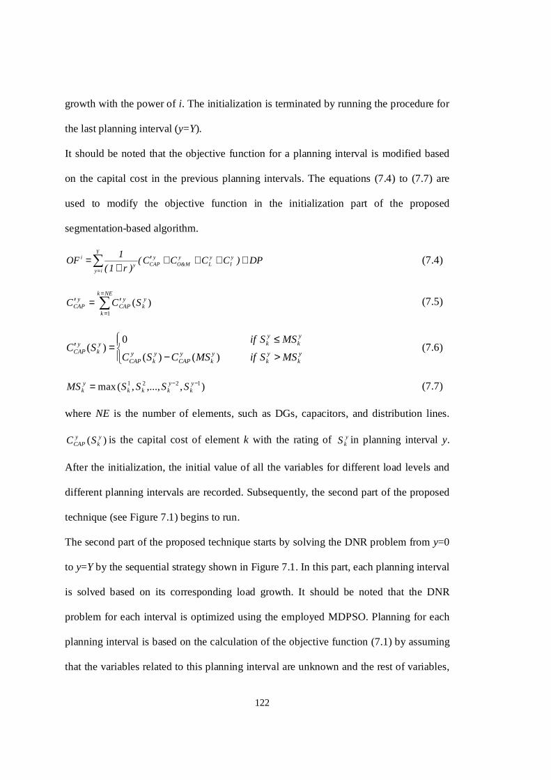
122
growth with the power of i. The initialization is terminated by running the procedure for
the last planning interval (y=Y).
It should be noted that the objective function for a planning interval is modified based
on the capital cost in the previous planning intervals. The equations (7.4) to (7.7) are
used to modify the objective function in the initialization part of the proposed
segmentation-based algorithm.
DP)CCCC()r1(
1OF
Y
iy
yI
yL
yM&O
yCAPy
i ++++′+
=∑=
(7.4)
∑=
=
′=′NEk
k
yk
yCAP
yCAP SCC
1
)(
(7.5)
>−
≤=′
yk
yk
yk
yCAP
yk
yCAP
yk
yky
ky
CAPMSSifMSCSC
MSSifSC
)()(
0)(
(7.6)
),,...,,(max 1221 −−= yk
ykkk
yk SSSSMS
(7.7)
where NE is the number of elements, such as DGs, capacitors, and distribution lines.
)( yk
yCAP SC is the capital cost of element k with the rating of y
kS in planning interval y.
After the initialization, the initial value of all the variables for different load levels and
different planning intervals are recorded. Subsequently, the second part of the proposed
technique (see Figure 7.1) begins to run.
The second part of the proposed technique starts by solving the DNR problem from y=0
to y=Y by the sequential strategy shown in Figure 7.1. In this part, each planning interval
is solved based on its corresponding load growth. It should be noted that the DNR
problem for each interval is optimized using the employed MDPSO. Planning for each
planning interval is based on the calculation of the objective function (7.1) by assuming
that the variables related to this planning interval are unknown and the rest of variables,
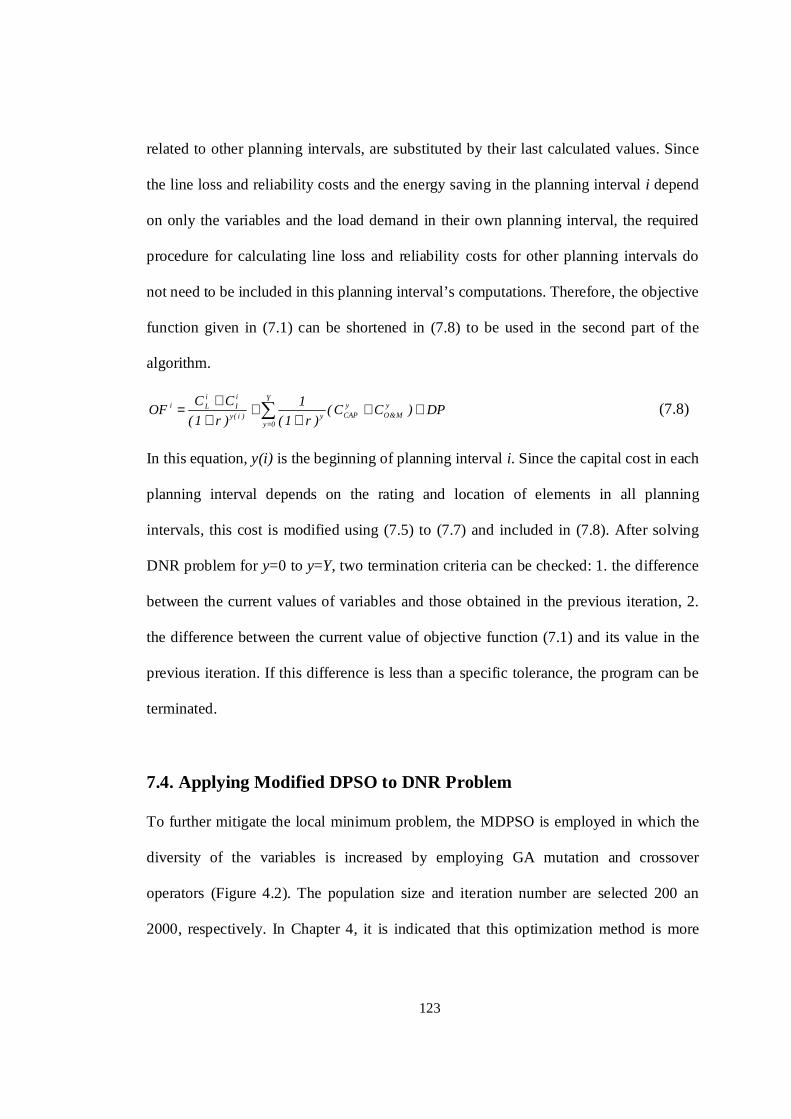
123
related to other planning intervals, are substituted by their last calculated values. Since
the line loss and reliability costs and the energy saving in the planning interval i depend
on only the variables and the load demand in their own planning interval, the required
procedure for calculating line loss and reliability costs for other planning intervals do
not need to be included in this planning interval’s computations. Therefore, the objective
function given in (7.1) can be shortened in (7.8) to be used in the second part of the
algorithm.
DP)CC()r1(
1
)r1(
CCOF
Y
0y
yM&O
yCAPy)i(y
iI
iLi ++
++
++= ∑
=
(7.8)
In this equation, y(i) is the beginning of planning interval i. Since the capital cost in each
planning interval depends on the rating and location of elements in all planning
intervals, this cost is modified using (7.5) to (7.7) and included in (7.8). After solving
DNR problem for y=0 to y=Y, two termination criteria can be checked: 1. the difference
between the current values of variables and those obtained in the previous iteration, 2.
the difference between the current value of objective function (7.1) and its value in the
previous iteration. If this difference is less than a specific tolerance, the program can be
terminated.
7.4. Applying Modified DPSO to DNR Problem
To further mitigate the local minimum problem, the MDPSO is employed in which the
diversity of the variables is increased by employing GA mutation and crossover
operators (Figure 4.2). The population size and iteration number are selected 200 an
2000, respectively. In Chapter 4, it is indicated that this optimization method is more

124
robust and accurate compared with some other optimization methods, such as
conventional DPSO, GA, SA, and DNLP.
Identification of the variables is the first stage in an optimization process. In this
methodology, these variables comprise the DG locations, active and reactive power of
DGs, capacitor locations and ratings, and VCT for different load levels. Furthermore,
the type of lines in each optimization planning interval is included. The particle which is
composed of the variables is shown in Figure 7.2. Given the rating of DGs and loads in
a planning interval, the apparent power which is required to be supplied by the HV/MV
transformer is calculated. This shows whether the transformer needs to be upgraded in
this planning interval.
Figure 7.2. The structure of a particle
7.5. Results
The 18-bus IEEE distribution system [19,100,123] is used (Figure 4.5) to validate the
proposed method. A five load level characteristic is used to approximate the load
duration curve in this chapter, helping to decrease the computation time. However, using
sensitivity analysis to find the load level number can be included as future research. It is
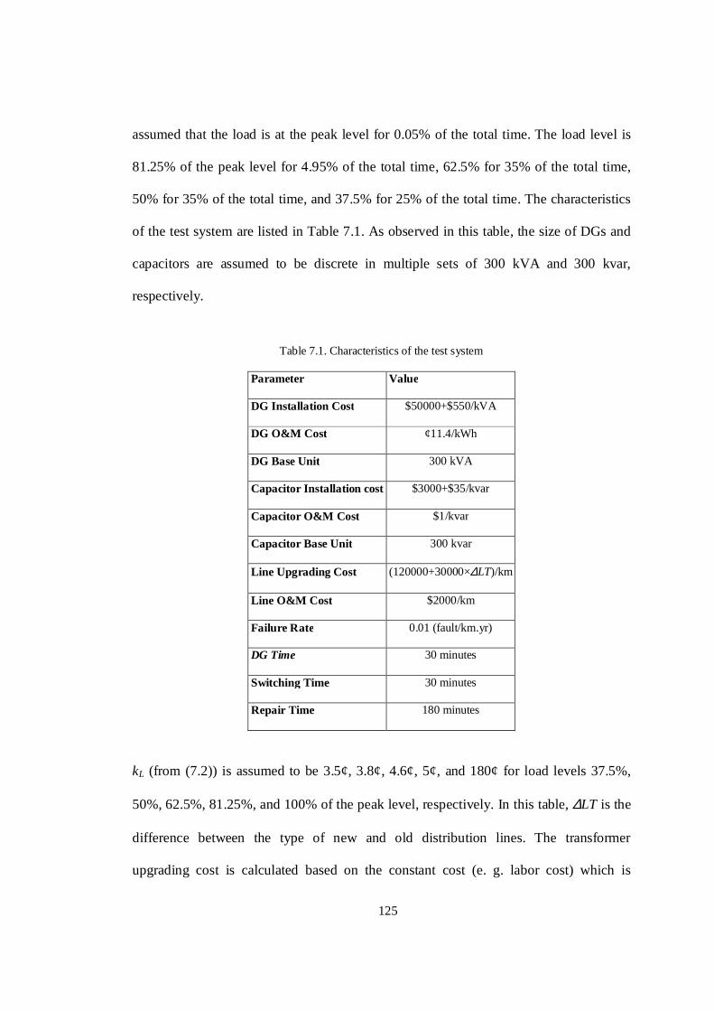
125
assumed that the load is at the peak level for 0.05% of the total time. The load level is
81.25% of the peak level for 4.95% of the total time, 62.5% for 35% of the total time,
50% for 35% of the total time, and 37.5% for 25% of the total time. The characteristics
of the test system are listed in Table 7.1. As observed in this table, the size of DGs and
capacitors are assumed to be discrete in multiple sets of 300 kVA and 300 kvar,
respectively.
Table 7.1. Characteristics of the test system
Parameter Value
DG Installation Cost $50000+$550/kVA
DG O&M Cost ¢11.4/kWh
DG Base Unit 300 kVA
Capacitor Installation cost $3000+$35/kvar
Capacitor O&M Cost $1/kvar
Capacitor Base Unit 300 kvar
Line Upgrading Cost (120000+30000×∆LT)/km
Line O&M Cost $2000/km
Failure Rate 0.01 (fault/km.yr)
DG Time 30 minutes
Switching Time 30 minutes
Repair Time 180 minutes
kL (from (7.2)) is assumed to be 3.5¢, 3.8¢, 4.6¢, 5¢, and 180¢ for load levels 37.5%,
50%, 62.5%, 81.25%, and 100% of the peak level, respectively. In this table, ∆LT is the
difference between the type of new and old distribution lines. The transformer
upgrading cost is calculated based on the constant cost (e. g. labor cost) which is

126
assumed to be $100000 and another cost which is based on the installation cost of the
new and old HV/MV transformers and related facilities. It is assumed that the old
transformer and associated facilities can be sold at half price.
Five different scenarios are studied in this section. In the first scenario, the conventional
planning method is applied. This scenario is improved by using capacitors in the second
scenario. DGs as a new technology are employed to plan the distribution system instead
of the conventional method in the third scenario. This technique is developed by using
capacitors in the fourth scenario. Finally, a comprehensive planning methodology
incorporating all technologies is studied in the fifth scenario.
It is assumed that the loads, located in the distribution network, are growing every five
years during the planning period (40% for the peak load level and 13% for other load
levels). Therefore, the planning interval is 5 years. As a result of this, four periods are
defined: Period 1 starts from first year and ends on fifth year, period 2 starts from sixth
year and ends on tenth year, period 3 starts from eleventh year and ends on fifteenth
year, and period 4 starts from sixteenth year and ends on twentieth year. The line
numbers are in this order, the line between buses, 1-2, 2-3, 3-4, 4-5, 5-6, 6-7, 7-8, 2-9, 1-
20, 20-21, 21-22, 21-23, 23-24, 23-25, and 25-26. Type of lines is as 6, 5, 5, 4, 1, 1, 1, 1,
3, 2, 1, 2, 1, 1, and 1 for line 1 to line 16 in order (Table 6.1). The load pattern and
growth is based on Queensland electricity network data [136].
7.5.1. Scenario 1 (Conventional Planning)
A conventional planning approach is studied in this scenario. Distribution networks are
commonly planned by upgrading the HV/MV transformer rating and line types. This is

127
mainly implemented for supporting the load growth. Additionally, it improves the line
loss and voltage profile. All these aspects are included in this scenario. For this purpose,
the objective function is composed of four parts, the line and transformer upgrading
costs, the line loss cost and the reliability cost. The bus voltages and feeder currents as
constraints should be limited into the standard level. Table 7.2 shows the results for
different periods in this scenario. In this table, the underlined numbers illustrate the lines
and transformer which are required to be upgraded due to the load growth in a period.
As shown in this table, 7 lines should be upgraded in period 2 to improve the voltage
profile and the line loss. This number is reduced to 6 in third period. The largest number
of lines requiring upgrading belongs to period 4 since the peak load level has the highest
value. The number of lines requiring upgrading can be reduced if another device can
assist the distribution lines by reducing the distribution lines flow.
Table 7.2. The line replacement in different periods (scenario 1)
Period Line Number Transformer
Rating (kVA) 1 2 3 4 5 6 7 8 9 10 11 12 13 14 15
1 6 5 5 4 1 1 1 1 3 2 1 2 1 1 1 25000
2 8 8 7 6 2 1 1 1 5 4 1 2 1 1 1 35000
3 10 10 9 7 2 1 1 1 5 5 1 5 1 1 1 50000
4 13 13 11 10 4 2 2 1 9 5 1 5 1 2 1 75000
To support the load growth, the HV/MV transformer needs to be upgraded in all periods
as no other devices are available to cooperate with the transformer. The main drawback
of the conventional planning is the excessive number of upgrading the line types and

128
transformer rating. To alleviate this, capacitors are employed in the next scenario to
decrease the line flows and to help the transformer by supporting a part of the load
growth.
7.5.2. Scenario 2 (Improved Conventional Planning)
The conventional planning method is improved in this scenario by installing capacitors.
Therefore, the objective function and constraints are similar to scenario one and the only
difference is that the capacitor investment cost is also included in the objective function.
The line types, transformer rating and capacitors for different periods are given in Figure
7.3 and Table 7.3.
Figure 7.3. The line types in different periods (scenario 2)
Similar to the previous table, the upgraded devices are shown by the underlined numbers
in this table. As observed in Figure 7.3, the number of lines requiring upgrading has
been reduced in this scenario. As an illustration, the number of line upgrading in period
1 2 3 4 5 6 7 8 9 10 11 12 13 14 150
2
4
6
8
10
12
Line Number
Lin
e T
ype
Period 4 Period 3 Period 2 Period 1

129
2 is 6 which is lower than previous scenario, 7. Similarly, this number has been
decreased from 6 to 5 in period 3 in this scenario compared with scenario 1.
Table 7.3. The capacitor replacement in different periods (scenario 2)
Period Bus Number Transformer
Rating (kVA) 4 6 7 9 20 21 23 25
1 0 0 600 0 0 0 0 600 25000
2 0 0 600 0 0 0 900 600 35000
3 0 2400 600 0 0 1200 1200 900 50000
4 3900 2400 2400 2100 900 1800 3000 3300 50000
Another benefit of this scenario compared with the previous one is that the HV/MV
transformer does not need to be upgraded every period. As shown in Table 7.3, this
transformer does not need to be upgraded in period 4. This is mainly because the
capacitors generate a part of the reactive power required for loads. The total apparent
power that the HV/MV transformer needs to supply is 58652 kVA when no capacitor is
available in the distribution network. As a result of this, a 75 kVA transformer was
required for period 4 in scenario 1 as the next available transformer after 50 kVA is 75
kVA. In the presence of capacitors, this power is reduced to 49969 kVA which makes
the 50 kVA transformer installed in the third period sufficient for the fourth period.
Table 7.3 demonstrates that two capacitors at buses 7 and 25 should be installed in the
first year. Another capacitor at bus 23 is then required to be employed in year 6. Two
more buses, 6 and 21, will have capacitors in year 11. Finally, buses 4, 9, and 20 will be
provided with a capacitor in year 16.
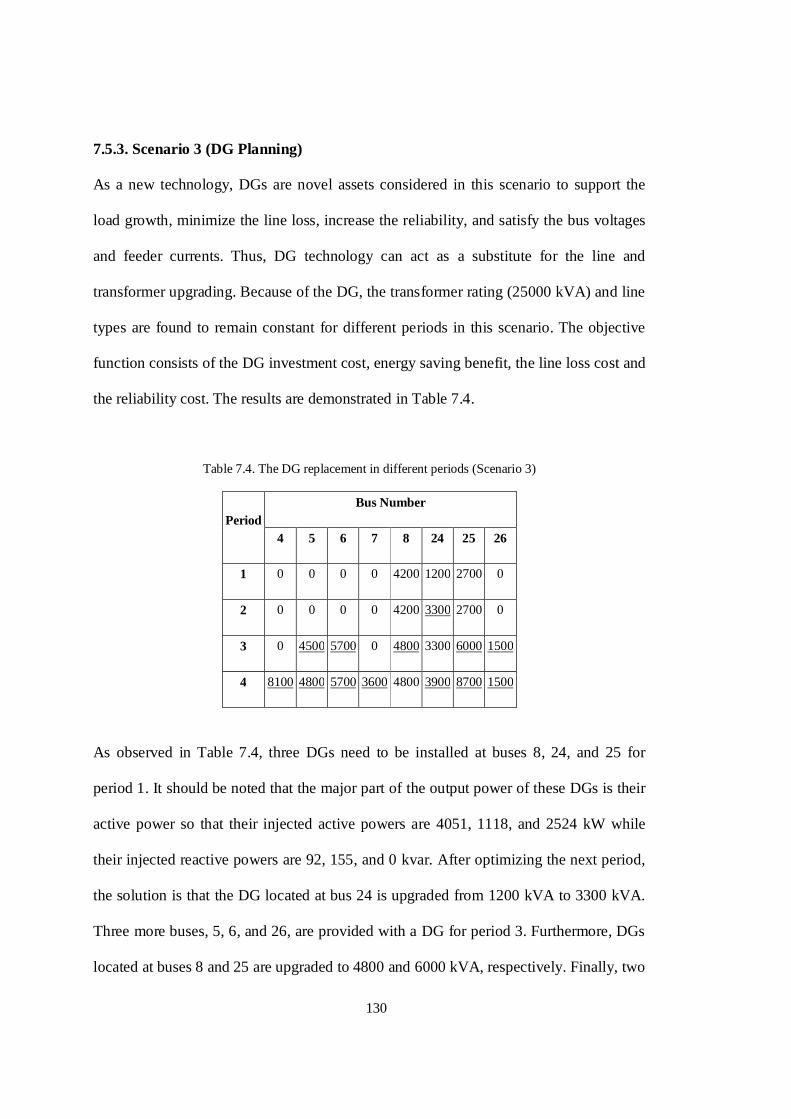
130
7.5.3. Scenario 3 (DG Planning)
As a new technology, DGs are novel assets considered in this scenario to support the
load growth, minimize the line loss, increase the reliability, and satisfy the bus voltages
and feeder currents. Thus, DG technology can act as a substitute for the line and
transformer upgrading. Because of the DG, the transformer rating (25000 kVA) and line
types are found to remain constant for different periods in this scenario. The objective
function consists of the DG investment cost, energy saving benefit, the line loss cost and
the reliability cost. The results are demonstrated in Table 7.4.
Table 7.4. The DG replacement in different periods (Scenario 3)
Period Bus Number
4 5 6 7 8 24 25 26
1 0 0 0 0 4200 1200 2700 0
2 0 0 0 0 4200 3300 2700 0
3 0 4500 5700 0 4800 3300 6000 1500
4 8100 4800 5700 3600 4800 3900 8700 1500
As observed in Table 7.4, three DGs need to be installed at buses 8, 24, and 25 for
period 1. It should be noted that the major part of the output power of these DGs is their
active power so that their injected active powers are 4051, 1118, and 2524 kW while
their injected reactive powers are 92, 155, and 0 kvar. After optimizing the next period,
the solution is that the DG located at bus 24 is upgraded from 1200 kVA to 3300 kVA.
Three more buses, 5, 6, and 26, are provided with a DG for period 3. Furthermore, DGs
located at buses 8 and 25 are upgraded to 4800 and 6000 kVA, respectively. Finally, two

131
more buses will have DGs in the last period. Moreover, the DGs located at buses 5, 24,
and 25 are upgraded. It is worth noting that the DG located at bus 26 does not need to
inject power in the fourth period. Therefore, it can be sold on sixteenth year.
The DGs, optimized in periods 1 to 3, operate only at peak load times, helping the
transformer by supporting the load growth. These generators do not operate at other load
levels since the benefit gained by minimizing the line loss in these load levels is not
sufficient compared with the fuel cost of DGs. Therefore, these DGs are switched on in
the non-peak load levels only to supply the loads when an outage occurs. For improving
the voltage profile in these load levels, the HV/MV transformer tap is set optimally. For
example, the VCT is optimized to be 0.99, 1.01, 1.01, 1.02, and 1.05 pu for different
load levels in period 2 or is set on 1.05 pu for all load levels in period 3.
As mentioned, the fuel cost of DGs is high which leads the solution not to use DGs in
non-peak load levels for reducing the line loss. In these low load times, capacitors, as
less expensive devices, can cooperate with DGs to decrease the line loss in non-peak
load times and to support a part of the load growth in the peak load times, thus
decreasing the required size of DGs, as more expensive devices, for this function. This
is considered in the following scenario.
7.5.4. Scenario 4 (Improved DG Planning)
The capacitors help DGs in this scenario to support the load growth and to minimize the
line loss. However, they do not have a considerable influence on the reliability as a part
of the objective function. Table 7.5 and Figure 7.4 show the capacitor and DG sizes and
locations in different periods, respectively. As observed, the total required DG is

132
decreased from 41100 kVA to 33900 kVA by using capacitors. This is a significant
benefit when the investment cost of DGs is much higher than capacitors.
The line and transformer upgrading is not included in scenarios 3 and 4. In order to find
a low cost planning, a compromise among installing DGs and capacitors, upgrading line
types and the HV/MV transformer needs to be done. This is implemented in the fifth
scenario.
Table 7.5. The capacitor replacement in different periods (Scenario 4)
Period Bus Number
2 3 4 5 9 20 22 23 25
1 1200 0 1200 1800 600 0 0 1500 0
2 900 1800 1200 1800 0 1800 0 0 0
3 2400 2100 600 0 2400 0 600 0 1200
4 900 300 2100 2700 0 0 0 0 2700
Figure 7.4. The DG rating in different periods (scenario 4)
4 5 6 7 8 23 24 25 260
500
1000
1500
2000
2500
3000
3500
4000
4500
5000
Bus Number
DG
Rat
ing
(kV
A)
Period 4 Period 3 Period 2 Period 1

133
7.5.5. Scenario 5 (Proposed Technique)
A comprehensive study considering all options is performed in this scenario. During the
optimization procedure, the variables are composed of the output active and reactive
power of DGs, rating of capacitors, and the VCT for different load levels and periods,
and the line types and transformer rating for different periods. The location of capacitors
and DGs are also obtained. The objective function is composed of the investment cost of
DGs, capacitors, lines, and transformer, the energy saving benefit, the line loss cost and
the network reliability cost. The results corresponding to this scenario for line and
transformer upgrades are given in Table 7.6.
Table 7.6. The line and transformer upgrades in different periods (Scenario 5)
Period Line Number Transformer
Rating (kVA) 1 2 3 4 5 6 7 8 9 10 11 12 13 14 15
1 6 5 5 4 1 1 1 1 3 2 1 2 1 1 1 25000
2 6 5 5 4 1 1 1 1 3 2 1 2 1 1 1 25000
3 11 9 9 6 3 1 1 1 5 5 1 2 1 1 1 50000
4 11 11 10 10 5 1 1 1 5 5 1 2 1 1 1 50000
As observed in Table 7.6, only one transformer upgrade is required at period 3. No line
upgrades are needed for the first two periods. However, seven lines are upgraded in the
third period which incurs much less cost compared with periods 1 and 2 as the net
present value of the cost is decreased after 11 years. Finally, lines 2, 3, 4, and 5 will be
upgraded in period 4 as the solution.
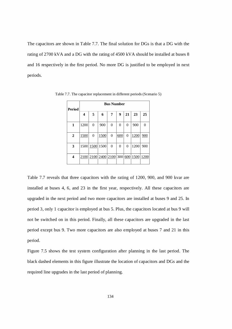
134
The capacitors are shown in Table 7.7. The final solution for DGs is that a DG with the
rating of 2700 kVA and a DG with the rating of 4500 kVA should be installed at buses 8
and 16 respectively in the first period. No more DG is justified to be employed in next
periods.
Table 7.7. The capacitor replacement in different periods (Scenario 5)
Period Bus Number
4 5 6 7 9 21 23 25
1 1200 0 900 0 0 0 900 0
2 1500 0 1500 0 600 0 1200 900
3 1500 1500 1500 0 0 0 1200 900
4 2100 2100 2400 2100 300 600 1500 1200
Table 7.7 reveals that three capacitors with the rating of 1200, 900, and 900 kvar are
installed at buses 4, 6, and 23 in the first year, respectively. All these capacitors are
upgraded in the next period and two more capacitors are installed at buses 9 and 25. In
period 3, only 1 capacitor is employed at bus 5. Plus, the capacitors located at bus 9 will
not be switched on in this period. Finally, all these capacitors are upgraded in the last
period except bus 9. Two more capacitors are also employed at buses 7 and 21 in this
period.
Figure 7.5 shows the test system configuration after planning in the last period. The
black dashed elements in this figure illustrate the location of capacitors and DGs and the
required line upgrades in the last period of planning.
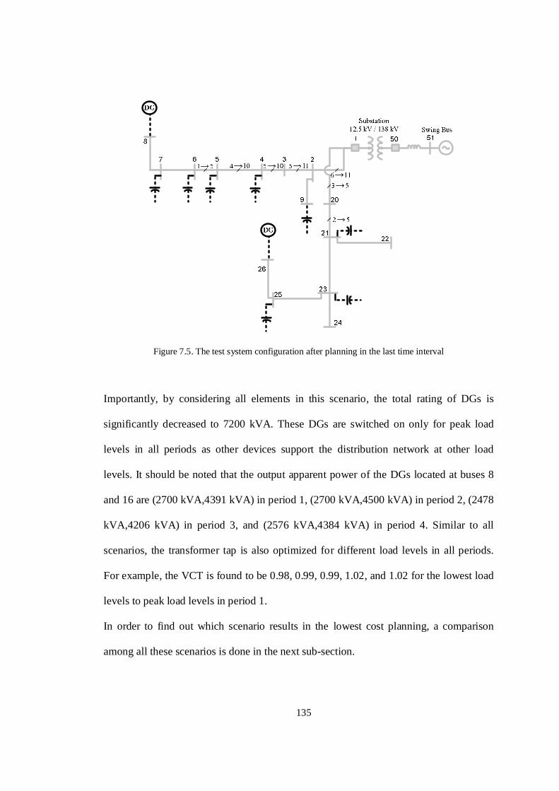
135
Figure 7.5. The test system configuration after planning in the last time interval
Importantly, by considering all elements in this scenario, the total rating of DGs is
significantly decreased to 7200 kVA. These DGs are switched on only for peak load
levels in all periods as other devices support the distribution network at other load
levels. It should be noted that the output apparent power of the DGs located at buses 8
and 16 are (2700 kVA,4391 kVA) in period 1, (2700 kVA,4500 kVA) in period 2, (2478
kVA,4206 kVA) in period 3, and (2576 kVA,4384 kVA) in period 4. Similar to all
scenarios, the transformer tap is also optimized for different load levels in all periods.
For example, the VCT is found to be 0.98, 0.99, 0.99, 1.02, and 1.02 for the lowest load
levels to peak load levels in period 1.
In order to find out which scenario results in the lowest cost planning, a comparison
among all these scenarios is done in the next sub-section.

136
7.5.6. Comparison of Different Scenarios
A variety of techniques for distribution network planning was implemented in scenarios
1 to 5. A conventional planning was studied in the first scenario. This technique was
improved by considering the capacitors in the second scenario. As a new coming
technology, DGs were planned to avoid upgrading the line and transformer upgrading in
scenario 3. This scenario was got better by including capacitors in the fourth scenario. A
comprehensive planning technique was finally presented in the fifth scenario in which
all technologies are incorporated. A comparison of the results for different scenarios is
shown in Table 7.8. All costs in this table are based on their net present value. The
economical results corresponding to scenario 5, as the proposed technique, for all
periods are given in Figure 7.6.
Table 7.8. Comparison of Total Cost during 20 years
Cost Elements Scenario Number
1 2 3 4 5
Line (M$) 1.66 1.524 0 0 0.728
Transformer (M$) 3.59 2.734 0 0 1.237
Capacitor (M$) 0 0.358 0 0.509 0.316
DG (M$) 0 0 13.588 11.731 4.096
Loss (M$) 0.813 0.761 1.202 1.094 0.874
Reliability (M$) 15.766 15.766 6.477 6.700 10.539
Energy Saving (M$) 0 0 -1.483 -1.359 -0.563
Total Cost (M$) 21.829 21.143 19.784 18.675 17.227

137
Figure 7.6. A summary of results for scenario 5
Table 7.8 reveals the main role of each element. As an illustration, the capacitors
employed in scenarios 2 reduce the loss cost and upgrading cost of transformer so that
these costs are $0.813M and $3.59M in scenario 1 which are reduced to $0.761M and
$2.734M by installing capacitors in scenario 2. Similarly, the line loss cost is decreased
from $1.202M to $1.094M in scenario 4 compared with scenario 3. The total cost
corresponding to the conventional planning is decreased $686000 by installing
capacitors. The total cost is also decreased from $19.784M to $18.675M in scenario 3
by installing the capacitors (scenario 4).
The main effect of DGs on the reliability is observed in scenarios 3 and 4 compared with
scenarios 1 and 2. The reliability cost in scenario 1 and 2 is $15.766M which is reduced
to about $6.5M in scenarios 3 and 4. On the other hand, this is observed that these
devices are not as appropriate as capacitors in minimizing the line loss so that this cost is
$0.813M in scenario 1 and is increased to $1.202M by installing DGs.
As revealed in Table 7.8, the highest total cost is related to the conventional planning in
which no capacitor and DG is included. After that, the second scenario suffers from high
Line Trans. Capa. DG Loss Reli. Energy Sav.10
3
104
105
106
107
Cost Elements
Co
st (
$)
Period 4 Period 3 Period 2 Period 1

138
total cost. This illustrates the significant role of DGs in planning distribution networks,
ultimately, planning techniques in which DGs are not included have higher total cost.
Using DGs can reduce the total cost by approximately 10% ($19.784M in scenario 3
compared with $21.829M in scenario 1 and $18.675M in scenario 4 compared with
$21.143M in scenario 2). Furthermore, using capacitors also decreases the total cost by
approximately 4% ($21.143M in scenario 2 compared with $21.829M in scenario 1 and
$18.675M in scenario 4 compared with $19.784M in scenario 3). The lowest cost plan is
associated with the technique proposed in this chapter, in which all technologies are
included, with a total cost of $17.277M. This demonstrates that the total cost related to
the conventional planning technique can be reduced 21% using the proposed technique.
As a conclusion, the total cost can be reduced $4.602M, $3.916M, $2.557M, and
$1.447M by using the proposed technique instead of the conventional planning (scenario
1), improved conventional planning (scenario 2), DG planning (scenario 3), and
improved DG planning (scenario 4), respectively.
7.6. Summary
In this chapter, a new methodology is proposed to perform the distribution network
reinforcement planning. This technique optimizes the following issues: 1) the line type,
2) transformer rating, 3) DG output active and reactive powers for all load levels, 4)
capacitor rating for all load levels, and 5) voltage on the customer side of HV/MV
transformer for all load levels. This optimization process results in supporting the annual
load growth, minimizing the line loss, maximizing the system reliability and improving
the voltage profile, all while minimizing construction costs. The bus voltage, line

139
current, and DG output power are constraints that should be within 5% of the rated
voltage, less than the rated current, and more than 30% of the rated power of DG,
respectively. This methodology is a segmentation-based approach for solving the
problems, which have a large number of variables. Given that the reliability cost and the
line loss cost associated with a planning year in the objective function only depend on
the variables in the corresponding planning year, the variables related to each planning
year is solved in a separate segment. Finally, the segments are solved sequentially to
solve the whole system. As a discrete problem, distribution network reinforcement is
approached using a MDPSO which is a modified version of DPSO. In this method, the
diversity of variables is increased which reduces the risk of trapping in the local minima.
Having considered a variety of scenarios, from traditional planning approaches to the
planning of a variety of assets, a number of conclusions can be made. The results
illustrate the importance of using capacitors in minimizing the line loss and preventing
the need for transformer upgrades, as a part of the loads are supported by capacitors.
Eventually, for the lowest cost, DGs must be included, where the main benefit of DGs is
to reduce the reliability cost and assist the transformer in meeting the load growth. It is
observed that the DGs are mainly required at the peak load level since the cost benefit
gained due to the line loss reduction by using DGs is less than the required fuel cost.
Ultimately, these outcomes demonstrate that the lowest cost planning results if the
proposed technique is used.

140

141
CHAPTER 8
A Comprehensive Reliability-Based Planning under
Load Growth
8.1. Introduction
A comprehensive planning approach was studied in previous chapter in which DGs were
employed chiefly for improving system reliability and supporting the load growth.
Although DGs improve system reliability significantly, their investment cost is an issue.
For alleviating this problem, less expensive elements, called cross-connections, are
employed in this chapter to help DGs for this goal. It should be noted that CCs are
primarily used in distribution networks located in urban and suburban areas where there
is short distance between buses which implies a reasonable cost for CCs. Here both DGs
and CCs are included in the optimization so the process can smoothly make transition
between urban and rural planning.
In this chapter, an integrated methodology is proposed for planning distribution
networks in which the operation of DGs and CCs is optimally planned. Distribution
lines and HV/MV transformers are also optimally upgraded. These are to improve
system reliability and to minimize line losses under load growth.
An objective function is constituted which is composed of the investment cost, loss cost,
and system reliability cost. The energy saving resulted by installing DGs is also included
in this function. The bus voltage and line current are maintained within their standard
142
bounds as constraints. As another constraint, the DG output power should not be less
than 30% of its rated power; otherwise, it is not switched on.
The MDPSO method, which was already described in chapter sub-section 4.3, is
employed in this chapter for optimizing this planning problem. To evaluate the proposed
approach, the distribution system connected to bus 4 of the RBTS is used. Four different
scenarios are assessed. In the first scenario, a basic planning approach is studied. In the
second scenario, the use of DG is planned to avoid the line and transformer upgrading.
In the third scenario, CC-based planning is studied when no DG exists. Finally, the
proposed technique, in which all technologies are included, is investigated in the fourth
scenario. The outcomes demonstrate that the lowest cost planning is resulted when all
technologies are incorporated.
8.2. Problem Formulation
In this section, the mathematical formulation of the proposed planning problem is
presented. The objective function is composed of system reliability, line losses, energy
saving and the investment cost as given in (7.1). As constraints, the bus voltage and the
feeder current should be maintained within the standard bounds and the DG output
power in a load level should be more than 30% of its rated power [134,135]. Converting
all of the objective function elements into the composite equivalent cost, this problem
can be solved using a single-objective optimization method. The objective function
which should be minimized is similar to (7.1).
The capital cost is composed of the cost for installing and purchasing DGs and CCs and
for upgrading lines and HV/MV transformers. It is mentioned that the CC investment

143
cost is calculated based on the length and conductor type of the corresponding CC and
the employed tie-switch cost. The operation and maintenance costs are self explanatory.
The distribution line loss cost is proportional to the energy lost on distribution lines. The
reliability cost is calculated based on the cost of energy not supplied.
The distribution line loss is converted into the composite equivalent cost using (7.2) and
the reliability cost is calculated using the total unsupplied demand after an outage as
given in (7.3). The energy saving (CES) is determined similar to the line loss cost, (7.2),
in which yll,LossP is replaced by the DG output active power for load level ll in the
planning interval y. The bus voltage and the feeder current, as constraints, should be
kept within the standard level as given in (3.6) and (3.7). The final constraint is the DG
output power, (6.5), which is required to be more than 30% of the rated power in all
times.
8.3. Methodology
To solve the planning problem considering that the load demand is growing, a sequential
algorithm is proposed as shown in Figure 7.1. This algorithm was described in sub-
section 7.3.
8.4. Applying Modified DPSO to Problem
The MDPSO, described in Chapter 4, is employed in this chapter for solving the
planning problem. The population size and iteration number are selected 300 an 2000,
respectively. Figure 8.1 shows the structure of variables associated with a planning
interval.

144
1 2 3 NB
DG Active Powers Cross-ConnectionsDG Reactive Powers Lines
. . . . . . . . . . . . . . . .
. . . . . . . . . . . . . . . .
. . . . . . . . . . . . . . . .
. . . . . . . .
. . . . . . . . . . . . . . . .
1 2 3 NB 1 2 3 NC 1 2 3 NL
1
LL
2
. . . . . . . . . . . . . . . . . . . . . . . . . . . . . . . .
Figure 8.1. The structure of a particle
In this figure, NB is the number of buses, NC is the number of CCs, and NL is the
number of distribution lines (almost similar to sub-section 7.4).
8.5. Results
To evaluate the proposed method, the distribution system connected to bus 4 of the
RBTS [89,137,138] is used. This network is composed of 3 HV/MV transformers with
the rating of 25, 15, 15 MVA which are supplying the loads using 7 main feeders. In this
chapter, the load duration curve is approximated in a four load level characteristic
helping to decrease the computation time. However, using sensitivity analysis to find the
number of load levels can be included in the future. The load is at the peak level for
0.05% of the total time. The load level is 81.25% of the peak level for 4.95% of the total
time, 62.5% for 65% of the total time, and 37.5% for 30% of the total time.
The characteristics of the test system are similar to listed in Table 7.1 except the CC
costs which are available in Table 8.1. In this table, ∆LT is the difference between the
type of new and old conductor and LT is the conductor type (Table 6.1). kL is assumed to

145
be 3.5¢, 4.6¢, 5¢, and 180¢ for load levels 37.5%, 62.5%, 81.25%, and 100% of the
peak level, respectively. The transformer upgrading cost is calculated based on a
constant cost (e. g. labor cost) which is assumed to be $100000 and another cost which
is based on the installation cost of the new and old HV/MV transformers and related
facilities (Table 6.2). It is assumed that the net cost of removal and sale of the old
transformer and associated facilities are half of the value quoted as the installation cost
in Table 6.2.
Similar to Chapter 6, the loads are assumed to grow every five years during the planning
period. This means that the planning interval is five years. Therefore, four periods are
required to be studied – one for each 5-year period.
Table 8.1. Characteristics of CCs
Parameter Value
CC Upgrading Cost (120000+30000×∆LT)/km
CC O&M Cost $2000/km
CC Installation Cost (180000+30000×LT)/km
It is assumed that all buses can be selected as a candidate for installing DGs and all lines
and transformers are capable of being upgraded. For CCs, a limited number of candidate
paths are selected based on the geographical and economical condition of the planning
area.
Four different scenarios are studied in this section. In the first scenario, a basic planning
is presented in which both distribution lines and HV/MV transformers are optimally
upgraded for supporting the load growth, decreasing the line loss, and improving the

146
voltage profile. In the second scenario, DGs as new technology are planned in the test
distribution system to improve the system reliability, line loss, and voltage profile and to
help the HV/MV transformers and distribution lines for supporting the load growth.
CCs, as reliability improver tools, along with the distribution lines are optimized in the
third scenario. Finally, an integrated planning methodology incorporating both DGs and
CCs is presented in the fourth scenario.
8.5.1. Scenario 1 (Basic Planning)
Distribution networks are basically planned by upgrading the HV/MV transformer
ratings and line types. This is mainly to support the load growth. Additionally, it
improves the line losses and voltage profile as the line impedance changes. Figure 8.2
shows the upgrading trend of HV/MV transformers.
Figure 8.2. The transformer ratings in different periods (scenario 1)
As observed in the above figure, the HV/MV transformers need to be upgraded in all
periods since no element such as DG is available in this planning for supporting the load
1 2 30
10
20
30
40
50
60
70
80
Transformer Number
Tra
nsf
orm
er R
atin
g (
MV
A)
Period 4 Period 3 Period 2 Period 1

147
growth. In addition to upgrading of transformers, the distribution lines need to be
upgraded excessively so that 13, 12, and 30 lines are re-rated in the second, third and
fourth periods, respectively. This extreme number of upgrades applies about $9.43M
and $3.46M as the net present value of the investment cost in transformers and lines.
DGs can be employed as alternatives for alleviating this issue as well as increasing the
system reliability as will be explained in the following sub-section.
8.5.2. Scenario 2 (DG Planning)
The future planning of distribution companies in many countries like Australia is to
increase the use of DGs in distribution networks. This is due to the large number of
benefits DGs have such as supporting the load growth and the peak load times,
improving the system reliability, mitigating the climate change, etc. In this chapter, DGs
are employed to help the transformers and lines for supporting the load growth and
escalating system reliability. Figure 8.3 shows the location and injection active, reactive,
and apparent power of DGs for the peak level in the last planning period.
Figure 8.3. The output power of DGs for the peak level in last period
11 17 19 27 30 42 45 49 51 55 56 58 64 65 680
1000
2000
3000
4000
5000
6000
7000
Bus Number
Po
wer
(kW
/kva
r,kV
A)
Apparent Power Active Power Reactive Power

148
As the final solution, fifteen DGs with the rating of 6900, 3300, 3600, 1800, 3900, 3600,
3300, 1800, 3300, 1800, 2400, 3600, 2100, 1800, and 2400 kVA are required to be
installed at buses 11, 17, 19, 27, 30, 42, 45, 49, 51, 55, 56, 58, 64, 65, and 68,
respectively.
It should be noted that the DG output powers in all load levels other than peak load level
are zero. This highlights the main benefit of DGs which is avoiding the upgrading of
transformers. It is observed that no line and transformer upgrade is required for the first
and second periods. For the third period, 4 lines are re-rated and still no transformer
upgrade is needed. The main re-rates are for the last period when 28 lines are upgraded
and the HV/MV transformers are upgraded to 35, 25, and 25 MVA, respectively.
Consequently, the investment cost in transformers and lines are reduced to $2.37M and
$2.24M by utilizing DGs. Furthermore, the reliability cost is decreased significantly
from $45.04M in the basic planning to $11.15M by including DGs in the planning
procedure. Although remarkable benefits are gained by using DGs, their large
investment cost is an issue so that the DG investment cost in this planning is calculated
to be $22.05M. Since major part of DGs are employed for improving the system
reliability, planning less expensive alternatives such as CCs is described in the
subsequent sub-section.
8.5.3. Scenario 3 (CC Planning)
In this scenario, CCs as less expensive devices compared with DGs, are employed to be
included in the basic planning. The required CCs in different periods are given in Table
8.2. The underlined values show that a CC needs to be upgraded.
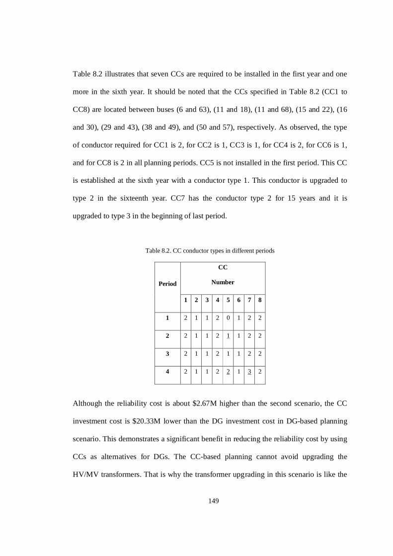
149
Table 8.2 illustrates that seven CCs are required to be installed in the first year and one
more in the sixth year. It should be noted that the CCs specified in Table 8.2 (CC1 to
CC8) are located between buses (6 and 63), (11 and 18), (11 and 68), (15 and 22), (16
and 30), (29 and 43), (38 and 49), and (50 and 57), respectively. As observed, the type
of conductor required for CC1 is 2, for CC2 is 1, CC3 is 1, for CC4 is 2, for CC6 is 1,
and for CC8 is 2 in all planning periods. CC5 is not installed in the first period. This CC
is established at the sixth year with a conductor type 1. This conductor is upgraded to
type 2 in the sixteenth year. CC7 has the conductor type 2 for 15 years and it is
upgraded to type 3 in the beginning of last period.
Table 8.2. CC conductor types in different periods
Period
CC
Number
1 2 3 4 5 6 7 8
1 2 1 1 2 0 1 2 2
2 2 1 1 2 1 1 2 2
3 2 1 1 2 1 1 2 2
4 2 1 1 2 2 1 3 2
Although the reliability cost is about $2.67M higher than the second scenario, the CC
investment cost is $20.33M lower than the DG investment cost in DG-based planning
scenario. This demonstrates a significant benefit in reducing the reliability cost by using
CCs as alternatives for DGs. The CC-based planning cannot avoid upgrading the
HV/MV transformers. That is why the transformer upgrading in this scenario is like the

150
basic planning. Additionally, the line investment cost is increased (from $3.46M to
$4.56 compared with the basic planning) since the rating of lines need to be enlarged to
help CCs in supplying more loads in a fault condition.
In order to support the load growth and reliability simultaneously, a comprehensive
planning is required as proposed in this chapter. The following sub-section presents the
results obtained by the proposed technique in which broad set of technologies are
included.
8.5.4. Scenario 4 (Proposed Integrated Planning)
In this section, an integrated planning is expressed which incorporates DGs and CCs
along with the lines and transformers upgrades. The main goal is to find the location as
well as the injection active and reactive power of DGs for different load levels, the
location and conductor type of CCs, and the upgrading of lines and HV/MV
transformers for different planning intervals under load growth. The objective function
is composed of the investment cost in these elements together with the line loss and
reliability costs and the energy saving due to using DGs. The test system configuration
after planning in the last period is shown in Figure 8.4. In this figure, the black dashed
elements are to illustrate the location of DGs and the required CCs in the last period of
planning.
The CC conductor types for different periods are given in Table 8.3. As observed in this
table, the placement and conductor type of the CCs installed in the first year is similar to
those obtained by the third scenario. In the second period, no CC is required to be
installed between buses 16 and 30 as it was in the CC-based planning scenario. CCs in
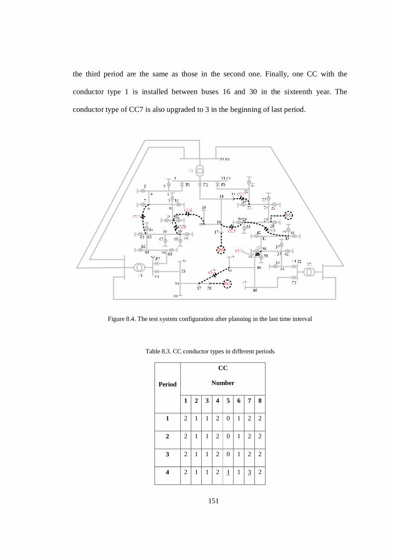
151
the third period are the same as those in the second one. Finally, one CC with the
conductor type 1 is installed between buses 16 and 30 in the sixteenth year. The
conductor type of CC7 is also upgraded to 3 in the beginning of last period.
CC8
Figure 8.4. The test system configuration after planning in the last time interval
Table 8.3. CC conductor types in different periods
Period
CC
Number
1 2 3 4 5 6 7 8
1 2 1 1 2 0 1 2 2
2 2 1 1 2 0 1 2 2
3 2 1 1 2 0 1 2 2
4 2 1 1 2 1 1 3 2

152
The CC investment cost is reduced from $1.72M to $1.62M if the proposed technique is
employed compared with the CC-based planning technique. Table 8.4 gives the
transformer ratings resulted by the proposed technique. This is observed that the number
of transformer upgrades decreases from 7 times to 5 times by combining both
technologies compared with the first and third scenarios. Furthermore, the transformer
ratings in different periods are lower than those obtained by non-DG based planning
scenarios (see Figure 8.2).
Table 8.4. The transformer ratings (MVA) in different periods (scenario 4)
Period Transformer Number
1 2 3
1 25 15 15
2 25 25 25
3 50 25 25
4 50 35 35
The rating of first transformer in the sixth year is 25 MVA in this scenario while it needs
to be upgraded to 35 MVA in the first and third scenarios. The same is for the third
transformer in the eleventh year. The rating of first and third transformers in the last
period is 75 and 50 MVA in the proposed technique while they are 50 and 35 MVA in
the non-DG based planning techniques. Totally, the transformer investment cost is
reduced from $9.43M to $5.93M compared with the non-DG based planning methods.
Similar to the second scenario, no DG is switched on for minimizing the line loss in load
levels other than the peak load level apart from running during faults for reliability

153
purposes. That these DGs are switched on for only the peak load times is to avoid
upgrading the HV/MV transformers.
The injection active, reactive, and apparent power of DGs at the peak load level along
with the DG ratings for different periods are given in Table 8.5.
Table 8.5. DG active, reactive, and apparent powers at peak load level (MVA) and DG ratings (MVA)
Period DG (bus =17) DG (bus =28) DG (bus =58)
P Q S P Q S P Q S
1 893 0 893 0 0 0 0 0 0
2 884 0 884 876 206 900 0 0 0
3 974 197 993 866 242 899 442 180 477
4 536 1124 1245 1427 386 1478 642 642 908
Rating
(MVA) 1500 1500 1200
As observed in Table 8.5, despite the second scenario in which 15 DGs are required to
be installed, the number of DGs in the fourth scenario is 3 so that the DG investment
cost is decreased extensively from $22.05M to $1.52M (about 93% cost reduction). The
results illustrate that three DGs with ratings 1500, 1500, and 1200 MVA are optimally
located at buses 17, 28, and 58, respectively. It should be noted that if the planning area
is rural with long distribution lines, the share of DGs will increase much more in the
provision of reliability since the CC investment cost will be large.
A summary of the economical results corresponding to scenario 4, as the proposed
technique, for all periods are given in Figure 8.5. It is mentioned that all costs in this

154
figure and all tables are based on the net present value. As observed in this figure, the
major part of the total cost is associated with the reliability cost and the transformer
investment cost. These costs are reduced considerably by using CCs and DGs
simultaneously compared with other scenarios.
Figure 8.5. A summary of results for the proposed planning
Table 8.6 shows a comparison among the results derived from different scenarios. As
observed in this table, planning based on DGs reduces the investment cost in distribution
lines so that the line cost in the second scenario is $2.24M which is about 65% of it in
the basic planning.
Comparing the line cost in the second, third and fourth scenarios illustrates that despite
DGs, using CCs lead to an increase in the line cost as the rating of lines need to be
raised to assist the CCs in supplying more loads in a fault condition as expected. The
outcomes illustrate that the reliability cost is significantly lessened by employing DGs
and CCs (from $45.04M by the basic planning method to $13.42M by the proposed
Line Transformer DG CC Reliability Loss Energy Saving10
3
104
105
106
Cost Elements
Co
st (
$)
Period 4 Period 3 Period 2 Period 1
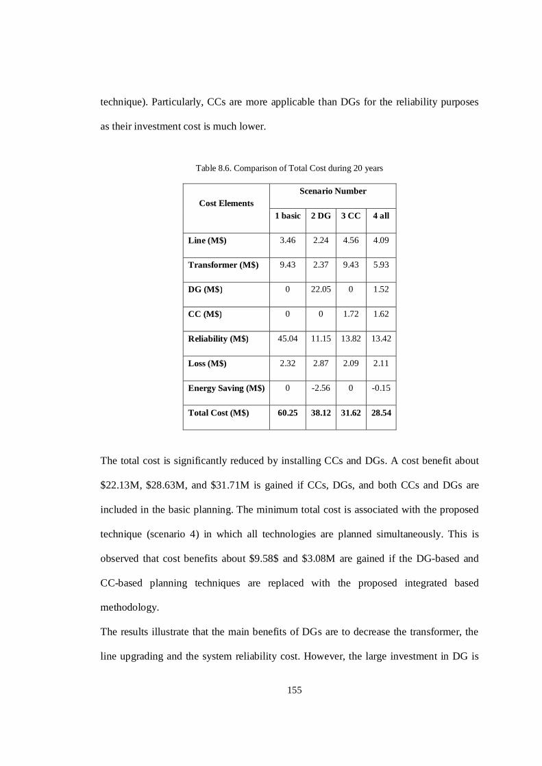
155
technique). Particularly, CCs are more applicable than DGs for the reliability purposes
as their investment cost is much lower.
Table 8.6. Comparison of Total Cost during 20 years
Cost Elements Scenario Number
1 basic 2 DG 3 CC 4 all
Line (M$) 3.46 2.24 4.56 4.09
Transformer (M$) 9.43 2.37 9.43 5.93
DG (M$) 0 22.05 0 1.52
CC (M$) 0 0 1.72 1.62
Reliability (M$) 45.04 11.15 13.82 13.42
Loss (M$) 2.32 2.87 2.09 2.11
Energy Saving (M$) 0 -2.56 0 -0.15
Total Cost (M$) 60.25 38.12 31.62 28.54
The total cost is significantly reduced by installing CCs and DGs. A cost benefit about
$22.13M, $28.63M, and $31.71M is gained if CCs, DGs, and both CCs and DGs are
included in the basic planning. The minimum total cost is associated with the proposed
technique (scenario 4) in which all technologies are planned simultaneously. This is
observed that cost benefits about $9.58$ and $3.08M are gained if the DG-based and
CC-based planning techniques are replaced with the proposed integrated based
methodology.
The results illustrate that the main benefits of DGs are to decrease the transformer, the
line upgrading and the system reliability cost. However, the large investment in DG is

156
an issue (See scenarios 2 and 4). CCs lessen the reliability cost significantly in a similar
way to DGs but with much lower cost. However, they increase the line investment cost
and cannot help the transformers to support the load growth (See scenario 3). These
aspects clarify why the integrated planning is required for a reliability-based planning
with minimum cost.
That DGs should be switched off for all load levels other than the peak load level
demonstrates that DGs are not justified for minimizing the line loss since the operation
and maintenance cost of DGs is more than the benefit gained from reducing the line
loss. That is why the line loss cost does not change remarkably by installing DGs as
observed in Table 8.6.
8.6. Summary
In this chapter, an integrated planning technique is proposed in which broad set of
technologies such as DGs and CCs are included to improve system reliability under load
growth. This planning determines the location and injection active and reactive power of
DGs for different load levels, the rating of lines and HV/MV transformers, and the
location and rating of CCs for different planning intervals.
To evaluate the proposed technique, the distribution system connected to bus 4 of the
RBTS is used. Four different scenarios are studied from basic planning approach to the
planning of a variety of assets.
The results illustrate that the main benefit of DGs is to avoid upgrading the HV/MV
transformers and distribution lines. The system reliability is also significantly improved
by installing DGs (75% cost reduction). Similarly, the transformer and line investment

157
costs are decreased about 75% and 35%, respectively. It is observed that DGs are
switched on only at the peak load level apart from running during faults for reliability
purposes since the benefit gained due to the line loss reduction is less than the required
fuel cost. On the other hand, CCs improves the system reliability almost as much as
DGs but with much lower investment cost particularly for urban networks. However,
they increase the line investment cost and cannot avoid upgrades of the transformers.
The outcomes demonstrate that inclusion of both technologies, DGs and CCs, reduces
the total cost significantly so that the lowest cost planning results if the proposed
integrated based technique is used.

158

159
CHAPTER 9
Conclusions and Recommendations
The conclusions of the thesis and recommendations for future work are presented in this
chapter.
9.1. Conclusions
A comprehensive approach to plan MV and LV distribution networks is the key
contribution presented in this thesis. First of all, a new configuration is proposed for
optimal allocation and sizing of distribution networks. A segmentation-based method is
proposed to decrease the size of the planning problem in which the optimal rating and
placement of distribution transformers and feeders for both MV and LV networks are
obtained sequentially. During this procedure, the line loss and reliability costs along
with the investment cost are minimized. This is demonstrated that the proposed
methodology is applicable to both uniform and non-uniform load densities. The
employed optimization method, DPSO, illustrates higher accuracy compared with GA
and identical results with the exhaustive search method. However, the exhaustive search
method is much more time consuming.
Since the objective function in planning problems is typically discrete and nonlinear,
using an appropriate optimization method is essential. Conventional optimization
approaches such as NLP ad DNLP usually work with continuous variables. However,
the real problems are discrete as the size of capacitor banks, DGs and transformers is
discrete. It has been found that these methods had a moderate probability of getting
160
stuck in local minima because of this discrete nature. The heuristic methods are reliable
alternatives for solving this type of discrete problems. In this thesis, a PSO-based
technique was developed through including some of the concepts in GA to provide
sufficient variability to avoid local minima. It has been found that this method, applied
to several distribution problems, is more robust and accurate compared with DNLP, GA,
SA, and DPSO for solving discrete and nonlinear problems such as the capacitor
planning.
As the voltage drop and line loss are two main concerns in distribution systems, almost
all distribution system devices which influence the voltage profile and the line loss,
VRs, LTCs, and capacitors, are incorporated for the first time in this research as the next
step of planning. A new segmentation-based strategy is contributed to find the location
and rating of these elements with reasonable accuracy and computation time where the
loads are practically assumed to have dynamic characteristics. It is illustrated that the
lowest cost planning is achieved by combining all the currently available technologies.
In addition to the line loss and voltage profile, the system reliability is another main
concern for distribution networks. For improving this index, DGs are involved in the
next step. An integrated planning is introduced for this purpose. During this procedure,
DGs and capacitors along with the distribution transformers and feeders are planned
simultaneously to improve the voltage profile, line loss, and system reliability. The
results highlight that the proposed integrated planning method results in the lowest
planning cost.
Another important factor which should be considered in planning problems is an index,
called load growth. For improving the system reliability along with line loss and voltage
161
profile as the load growth is supported, a new arrangement is contributed for allocation
and sizing of DGs along with capacitors while the distribution transformers and feeders
are planned under load growth. For inclusion of the load growth factor, a segmentation-
based strategy is innovated. This segmentation-based strategy is then employed in a new
integrated method for performing a comprehensive planning to minimize the line loss
cost, the reliability cost, and the investment cost simultaneously and to improve the
voltage profile under load growth. In order to avoid using extra DGs, as extremely
expensive elements, CCs are employed for increasing the system reliability. The
outcomes demonstrate that inclusion of both technologies, DGs and CCs, reduces the
total cost significantly so that the lowest cost planning results if the proposed integrated
based technique is used.
The results illustrate that the main benefit of DGs is to avoid upgrading the HV/MV
transformers and distribution lines. It is also observed that DGs are required to be
switched on only at the peak load level apart from running during faults for reliability
purposes since the benefit gained due to the line loss reduction is less than the required
fuel cost. On the other hand, capacitors are lower-expensive alternatives for minimizing
the line loss, improving the voltage profile, and preventing the need for transformer
upgrades, as a part of the loads are supported by capacitors. From system reliability
viewpoint, CCs improve reliability indices almost as much as DGs but with much lower
investment cost particularly for urban networks. However, they increase the line
investment cost and cannot avoid upgrades of the distribution transformers. This
demonstrates that, for the lowest cost planning, DGs must be included, to reduce the
reliability cost and chiefly to assist the transformer in meeting the load growth.
162
Ultimately, compared with the traditional planning approaches, the outcomes
demonstrate that the lowest cost planning results if the proposed technique is used and
all available technologies are included.
Given that the reliability and line loss cost in a planning year only depend on the rating
and placement of elements in the corresponding planning year, variables associated with
a planning year are more sensitive to each other rather than to variables in the other
planning years. Therefore, a segmentation-based algorithm was proposed to categorize
the variables into different segments (each segment is associated with a planning year).
Then the segments are solved sequentially to find a solution for whole system in a lower
time compared with exhaustive search. The above mentioned planning strategies are
reasonably applicable for a medium-scale network. However, if the planning network
has a large-scale, applying a reliable segmentation-based algorithm is required which is
pointed out in the future work.
9.2. Recommendations for Future Research
The following future works are recommended:
9.2.1. Integration of Different Types of DGs
In this research, the type of DGs is also optimized based on the geographical
characteristic of the planning area. For this purpose, each candidate location is identified
using a variety of geographical coefficients for different types of DGs and the
optimization program optimize the desired DG.

163
9.2.2. Inclusion of the Stability Index in the Wind turbine Planning
This research focuses on optimizing the injecting power of wind turbine generators
based on the load duration curve and wind characteristics while the network stability
when the wind turbine is suddenly disconnected is maintained.
9.2.3. Consideration of Power Quality in the DG Planning
Another benefit of using DGs is to improve the power quality. This index can be
satisfied as the DG is improving the line loss, voltage profile, system reliability, and the
load growth support.
9.2.4. Using Large-Scale Optimization Method for Distribution Network Planning
Since the practical distribution networks are quite large, the number of candidate buses
so the number of variables is remarkable. Optimizing a large system may result in
significant decrease of the accuracy and increase of the computation time. For solving
this issue, segmentation procedure can be applicable. For this purpose, a sensitivity
analysis can be applied to find the dependant variables. It is obvious that a correct
segmentation can decrease the computation time while the accuracy decreases
negligibly. Among the segmentation-based methods, Benders Decomposition method
has presented acceptable results [139]. This method is employed extensively in the
power system literature, such as in unit commitment [140], electricity market [141],
hydrothermal scheduling [142], and distribution systems reconfiguration [143]. Benders
Decomposition method is originally applied when integer variables (particularly binary
variable) and continuous variables exist in the optimization problem. In this method, the

164
continuous and discrete variables are manipulated separately in two different stages. The
first stage, called master, deals with the discrete variables and the second stage, called
slave, is to solve the continuous variables.

165
References
[1] D. L. Wall, G. L. Thompson, J. E. D. Northcote-Green, “An Optimization Model for Planning
Radial Distribution Networks”, IEEE Transactions on Power Apparatus and Systems, Vol. 98, No.
3, May/June 1979, PP. 1061-1068.
[2] G. L. Thompson, D. L. Wall, “A Branch and Bound Model for Choosing Optimal Substation
Locations”, IEEE Transactions on Power Apparatus and Systems, Vol. 100, No. 5, May 1981, PP.
2683-2688.
[3] D. I. Sun, D. R. Farris, P. J. Cote, “Optimal Distribution Substation and Primary Feeder Planning
via the Fixed Charge Network Formulation”, IEEE Transactions on Power Apparatus and Systems,
Vol. 101, No. 3, March 1982, PP. 602-609.
[4] T. H. Fawzi, K. F. Ali, S. M. El-Sobki, “A New Planning Model for Distribution Systems”, IEEE
Transactions on Power Apparatus and Systems, Vol. 102, No. 9, September 1983, PP. 3010-3017.
[5] M. A. El-Kady, “Computer-Aided Planning of Distribution Substation and Primary Feeders”, IEEE
Transactions on Power Apparatus and Systems, Vol. 103, No. 6, June 1984, PP. 1183-1189.
[6] J. Boardman, C. Meckiff, “A Branch and Bound Formulation to An Electricity Distribution
Planning Problem”, IEEE Transactions on Power Apparatus and Systems, Vol. 104, No. 8, August
1985, PP. 2112-2118.
[7] H. K. Youssef, R. Hackam, M. A. Abu-El-Maghd, “Novel Optimization Model for Long Range
Distribution Planning”, IEEE Transactions on Power Apparatus and Systems, Vol. 104, No. 11,
November 1985, PP. 3195-3202.
[8] T. Gönen, I. J. Ramirez-Rosado, “Optimal Multi-Stage Planning of Power Distribution Systems”,
IEEE Transactions on Power Delivery, Vol. 2, No. 2, April 1987, PP. 512-519.
[9] A. C. Marshall, T. B. Boffey, J. R. Green, “Optimal Design of Electricity Distribution Networks”,
IEE Proceedings Generation, Transmission and Distribution, Vol. 138, No. 1, January 1991, PP.
69-77.

166
[10] E. Miguez, J. Cidras, E. Diaz-Dorado, “An Improved Branch-Exchange Algorithm for Large-Scale
Distribution Network Planning”, IEEE Transactions on Power Systems, Vol. 17, No. 4, November
2002, PP. 931-936.
[11] V. Miranda, J. V. Ranito, L. M. Proenca, “Genetic Algorithms in Optimal Multistage Distribution
Network Planning”, IEEE Transactions on Power Systems, Vol. 9, No. 4, November 1994, PP.
1927-1933.
[12] S. K. Goswami, “Distribution System Planning Using Branch Exchange Technique”, IEEE
Transactions on Power Systems, Vol. 12, No. 2, May 1997, PP. 718-723.
[13] E. Diaz-Dorado, Jose Cidars, E. Miguez, “Application of Evolutionary Algorithms for the Planning
of Urban Distribution Networks of Medium Voltage”, IEEE Transactions on Power Systems, Vol.
17, No. 3, August 2002, PP. 879-884.
[14] J. F. Gomez, H. Khodr, P. Oliviera, L. Ocque, “Ant Colony System Algorithm for the Planning of
Primary Distribution Networks”, IEEE Transactions on Power Systems, Vol. 19, No. 2, May 2004,
PP. 996-1004.
[15] V. Parada, J. A. Ferland, M. Arias, “Optimization of Electrical Distribution Feeders Using
Simulated Annealing”, IEEE Transactions on Power Delivery, Vol. 19, No. 3, July 2004, PP.
1135-1141.
[16] I. J. Ramirez-Rosado, J. A. Dominguez-Navarro, “New Multiobjective Tabu Search Algorithm for
Fuzzy Optimal Planning of Power Distribution Systems”, IEEE Transactions on Power Systems,
Vol. 21, No. 1, February 2006, PP. 224-233.
[17] F. Mendoza, J. L. Bernal-Agustin, J. A. Dominguez-Navarro, “NSGA and SPEA Applied to
Multiobjective Design of Power Distribution Systems”, IEEE Transactions on Power Systems,
Vol. 21, No. 4, November 2006, PP. 1983-1945.
[18] J. M. Nahman, D. M. Peric, “Optimal Planning of Radial Distribution Networks by Simulated
Annealing Technique”, IEEE Transactions on Power Systems, Vol. 23, No. 2, May 2008, PP. 790-
795.
[19] S. Najafi, S. H. Hosseinian, M. Abedi, “A Framework for Optimal Planning in Large Distribution
Networks”, IEEE Transactions on Power Systems, Vol. 24, No. 2, May 2009, PP. 1019-1028.
167
[20] D. M. Crawford, S. B. Holt, “A Mathematical Optimization Technique for Locating and Sizing
Distribution Substations, and Deriving their Optimal Service Areas”, IEEE Transactions on Power
Apparatus and Systems, Vol. 94, No. 2, March/April 1975, PP. 230-235.
[21] M. Kaplan, A. Braunstein, “Contribution to the Determination of the Optimum Site for
Substations”, IEEE Transactions on Power Apparatus and Systems, Vol. 100, No. 5, May 1981,
PP. 2263-2270.
[22] T. H. Fawzi, K. F. Ali, S. M. El-Sobki, “Routing Optimization of Primary Rural Distribution
Feeders”, IEEE Transactions on Power Apparatus and Systems, Vol. 101, No. 5, May 1982, PP.
1129-1133.
[23] M. Ponnavaikko, K. S. Prakasa Rao, “An Approach to Optimal Distribution System Planning
through Conductor Gradation”, IEEE Transactions on Power Apparatus and Systems, Vol. 101,
No. 6, June 1982, PP. 1735-1742.
[24] H. L. Willis, J. E. D. Northcote-Green, “Comparison of Several Computerized Distribution
Planning Methods”, IEEE Transactions on Power Apparatus and Systems, Vol. 104, No. 1, January
1985, PP. 233-240.
[25] T. Gönen, I. J. Ramirez-Rosado, “Review of Distribution System Planning Models: A Model for
Optimal Multistage Planning”, IEE Proceedings Generation, Transmission and Distribution, Vol.
133, No. 7, November 1986, PP. 397-408.
[26] M. Ponnavaikko, K. S. Prakasa Rao, S. S. Venkata, “Distribution System Planning through A
Quadratic Mixed Integer Programming Approach”, IEEE Transactions on Power Delivery, Vol. 2,
No. 4, October 1987, PP. 1157-1163.
[27] I. J. Ramirez-Rosado, T. Gönen, “Pseudodynamic Planning for Expansion of Power Distribution
Systems”, IEEE Transactions on Power Systems, Vol. 6, No. 1, February 1991, PP. 245-254.
[28] A. Benchakroun, J. A. Ferland, R. Cleroux, “Distribution System Planning through a Generalized
Benders Decomposition Approach”, European Journal of Operational Research, Vol. 62, Issue 2,
October 1992, PP. 149-162.

168
[29] V. H. Quintana, H. K. Temraz, K. W. Hipel, “Two-Stage Power System Distribution Planning
Algorithm”, IEE Proceedings Generation, Transmission and Distribution, Vol. 140, No. 1, January
1993, PP. 17-29.
[30] M. Carneiro S, P. M. Franca, P. D. Silveira, “Long-Range Planning of Power Distribution
Systems: Primary Networks”, Electric Power Systems Research, Vol. 27, Issue 3, August 1993,
PP. 223-231.
[31] K. Nara, H. Kuwabara, M. Kitagawa, K. Ohtaka, “Algorithm for Expansion Planning in
Distribution Systems Taking Faults into Consideration”, IEEE Transactions on Power Systems,
Vol. 9, No. 1, February 1994, PP. 324-330.
[32] K. L. Lo, I. Nashid, “Interactive Expert System for Optimal Design of Electricity Distribution
Systems”, IEE Proceedings Generation, Transmission and Distribution, Vol. 143, No. 2, March
1996, PP. 151-156.
[33] I. J. Ramirez-Rosado, J. L. Bernal-Agustin, “Genetic Algorithm Applied to Design of Large
Power-Distribution Systems”, IEEE Transactions on Power Systems, Vol. 13, No. 2, May 1998,
PP. 696-703.
[34] P. Singh, E. B. Makram, W. P. Adams, “A New Technique for Optimal Time-Dynamic
Distribution Substation and Feeder Planning”, Electric Power Systems Research, Vol. 47, Issue 3,
November 1998, PP. 197-204.
[35] M. A. Farrag, M. M. El-Metwally, M. S. El-Bages, “A New Model for Distribution System
Planning”, International Journal of Electrical Power and Energy Systems, Vol. 21, Issue 7, October
1999, PP. 523-531.
[36] R. Ranjan, B. Venkatesh, D. Das, “A New Algorithm for Power Distribution System Planning”,
Electric Power Systems Research, Vol. 62, Issue 1, May 2002, PP. 55-65.
[37] T. H. M. El-Fouly, H. H. Zeineldin, E. F. El-Saadany, “A New Optimization Model for
Distribution Substation Siting, Sizing, and Timing”, International Journal of Electrical Power and
Energy Systems, Vol. 30, Issue 5, June 2008, PP. 308-315.

169
[38] M. C. Da Silva, P. M. Franca, P. D. B. Da Silveira, “Long-Range Planning of Power Distribution
Systems: Secondary Networks”, Computers and Electrical Engineering, Vol. 22, Issue 3, May
1996, PP. 179-191.
[39] E. Diaz-Dorado, E. Miguez, J. Cidars, “Design of Large Rural Low-Voltage Networks Using
Dynamic Programming Optimization”, IEEE Transactions on Power Systems, Vol. 16, No. 4,
November 2001, PP. 898-903.
[40] E. Diaz-Dorado, J. C. Pidre, E. M. Garcia, “Planning of Large Rural Low-Voltage Networks Using
Evolution Strategies”, IEEE Transactions on Power Systems, Vol. 18, No. 4, November 2003, PP.
1594-1600.
[41] A. M. Cossi, R. Romero, J. R. S. Mantovani, “Planning of Secondary Distribution Circuits through
Evolutionary Algorithms”, IEEE Transactions on Power Delivery, Vol. 20, No. 1, January 2005,
PP. 205-213.
[42] J. Shao, N. D. Rao, Y. Zhang, “An Expert System for Secondary Distribution System Design”,
IEEE Transactions on Power Delivery, Vol. 6, No. 4, October 1991, PP. 1607-1615.
[43] D. M. Jovanovic, “Planning of Optimal Location and Sizes of Distribution Transformers Using
Integer Programming”, International Journal of Electrical Power and Energy Systems, Vol. 25,
Issue 9, November 2003, PP. 717-723.
[44] A. S. Safigianni, “Optimization of a Secondary Power Distribution System”, International Journal
of Electrical Power and Energy Systems, Vol. 27, Issue 2, February 2005, PP. 131-138.
[45] A. Navarro, H. Rudnick, “Large-Scale Distribution Planning - Part I: Simultaneous Network and
Transformer Optimization”, IEEE Transactions on Power Systems, Vol. 24, No. 2, May 2009, PP.
744-751.
[46] A. Navarro, H. Rudnick, “Large-Scale Distribution Planning - Part II: Macro-Optimization with
Voronoi’s Diagram and Tabu Search”, IEEE Transactions on Power Systems, Vol. 24, No. 2, May
2009, PP. 752-758.
[47] P. C. Paiva, H. M. Khodr, J. A. Dominguez-Navarro, “Integral Planning of Primary-Secondary
Distribution Systems Using Mixed Integer Linear Programming”, IEEE Transactions on Power
Systems, Vol. 20, No. 2, May 2005, PP. 1134-1143.
170
[48] R. H. Fletcher, K. Strunz, “Optimal Distribution System Horizon Planning-Part I: Formulation”,
IEEE Transactions on Power Systems, Vol. 22, No. 2, May 2007, PP. 791-799.
[49] R. H. Fletcher, K. Strunz, “Optimal Distribution System Horizon Planning-Part II: Application”,
IEEE Transactions on Power Systems, Vol. 22, No. 2, May 2007, PP. 862-870.
[50] M. R. Alrashidi, M. E. El-Hawary, “A Survey of Particle Swarm Optimization Applications in
Electric Power Systems”, IEEE Transactions on Evolutionary Computation, Vol. 13, No. 4, August
2009.
[51] Y. Del Valle, G. K. Venayagamoorthy, S. Mohagheghi, “Particle Swarm Optimization: Basic
Concepts, Variants and Applications in Power Systems”, IEEE Transactions on Evolutionary
Computation”, Vol. 12, No. 2, April 2008, PP. 171-195.
[52] A.S. Safigianni, G. J. Salis, “Optimum Voltage Regulator Placement in a Radial Power
Distribution Network”, IEEE Transactions on Power Systems, Vol. 15, No. 2, May 2000, PP. 879-
886.
[53] J. E. Mendoza, D. A. Morales, R. A. Lopez, “Multiobjective Location of Automatic Voltage
Regulators in a Radial Distribution Network Using a Micro Genetic Algorithm”, IEEE
Transactions on Power Systems, Vol. 22, No. 1, February 2007, PP. 404-412.
[54] C. F. Chang, “Reconfiguration and Capacitor Placement for Loss Reduction of Distribution
Systems by Ant Colony Search Algorithm”, IEEE Transactions on Power Systems, Vol. 23, No. 4,
November 2008, 1747-1755.
[55] M. A. S. Masoum, M. Ladjevardi, A. Jafarian, “Optimal Placement, Replacement and Sizing of
Capacitor Banks in Distorted Distribution Networks by Genetic Algorithms”, IEEE Transactions
on Power Delivery, Vol. 19, No. 4, November 2008, 1794-1801.
[56] M. Ladjevardi, M. A. S. Masoum, “Genetically Optimized Fuzzy Placement and Sizing of
Capacitor Banks in Distorted Distribution Networks”, IEEE Transactions on Power Delivery, Vol.
23, No. 1, January 2008, 449-456.
[57] Z. Q. Wu, K. L. Lo, “Optimal Choice of Fixed and Switched Capacitors in Radial Distributors with
Distorted Substation Voltae”, IEE Proceedings of Generation, Transmission and Distribution, Vol.
142, No. 1, January 1995, PP. 24-28.

171
[58] G. Levitin, A. Kalyuzhny, A. Shenkman, “Optimal Capacitor Allocation in Distribution Systems
Using a Genetic Algorithm and a Fast Energy Loss Computation Technique”, IEEE Transactions
on Power Delivery, Vol. 15, No. 2, April 2000, PP. 623-628.
[59] S. Sundhararajan, A. Pahwa, “Optimal Selection of Capacitors for Radial Distribution Systems
Using a Genetic Algorithm”, IEEE Transactions on Power Systems, Vol. 9, No. 3, August 1994,
PP. 1499-1507.
[60] M. E. Baran, F. F. Wu, “Optimal Capacitor Placement on Radial Distribution Systems”, IEEE
Transactions on Power Delivery, Vol. 4, No. 1, January 1989, PP. 725-734.
[61] M. E. Baran, F. F. Wu, “Optimal Sizing of Capacitor Placed on a Radial Distribution System”,
IEEE Transactions on Power Delivery, Vol. 4, No. 1, January 1989, PP. 735-743.
[62] M. B. Liu, C. A. Canizares, W. Huang, “Reactive Power and Voltage Control in Distribution
Systems with Limited Switching Operations”, IEEE Transactions on Power Systems, Vol. 24, No.
2, May 2009, PP. 889-899.
[63] R. H. Liang, C. K. Cheng, “Dispatch of Main Transformer ULTC and Capacitors in a Distribution
System”, IEEE Transactions on Power Delivery, Vol. 16, No. 4, October 2001, PP. 625-630.
[64] A. Ulinuha, M. A. S. Masoum, S. M. Islam, “Optimal Scheduling of LTC and Shunt Capacitors in
Large Distorted Distribution Systems Using Evolutionary-Based Algorithms”, IEEE Transactions
on Power Delivery, Vol. 23, No. 1, January 2008, PP. 434-441.
[65] R. Ramakumar, “Renewable Energy Sources and Developing Countries”, IEEE Transaction on
Power Apparatus and Systems, Vol. PAS-102, No. 2, February 1983, PP. 502-510.
[66] P. Chiradeja, R. Ramakumar, “An Approach to Quantify the Technical Benefits of Distributed
Generation”, IEEE Transaction on Energy Conversion, Vol. 19, No. 4, December 2004, PP. 764-
773.
[67] S. R. Bull, “Renewable Energy Today and Tomorrows”, Proceedings of the IEEE, Vol. 89, No. 8,
August 2001, PP. 1216-1226
[68] J. E. J. Cottrill, “Economic Assessment of the Renewable Energy Sources”, IEE Proceedings on
Physical Science, Measurement and Instrumentation, Management and Education, Vol. 127, Pt. A,
No. 5, June 1980, PP. 279 – 288.
172
[69] S. A. Farghal, M. Roshdy Abdel Aziz, “Generation Expansion Planning Including the Renewable
Energy Sources”, IEEE Transaction on Power System, Vol. 3, No. 3, August 1988, PP. 816-822.
[70] H. B. Puttgen, P. R. Macgregor, F. C. Lambert, “Distributed Generation: Semantic hype or the
Dawn of a new Era?”, IEEE Power and Energy Magazine, January/February 2003, PP. 22-29.
[71] B. Norton, “Renewable Electricity- What is the True Cost?”, Power Engineering Journal, Vol. 13,
Issue 1, February 1999, PP. 6-12.
[72] C. Wang, M. H. Nehrir, “Analytical Approaches for Optimal Placement of Distributed Generation
Sources in Power Systems”, IEEE Transaction on Power System, Vol. 19, No. 4, November 2004,
PP. 2068-2076.
[73] D. H. Popovic, J. A. Greatbanks, M. Begovic, “Placement of Distributed Generators and Reclosers
for Distribution Network Security and Reliability”, International Journal of Electrical Power and
Energy Systems, Vol. 27, Issues 5-6, June-July 2005, PP. 398-408.
[74] N. Mithulananthan, T. Oo, Le Van Phu, “Distributed Generator Placement in Power Distribution
System Using Genetic Algorithm to Reduce Losses”, Thammasat International Journal of Science
and Technology, Vol. 9, No. 3, July-September 2004, PP. 55-62.
[75] H. Shim, Jung-Hoon Park, In-Su Bae, “Optimal Capacity and Allocation of Distributed Generation
by Minimum Operation Cost in Distribution Systems”, KIEE International Transactions on Power
Engineering, Vol. 5-A, No. 1, 2005, PP. 9-15.
[76] G. Celli, E. Ghiani, S. Mocci, and F. Pilo, “A Multiobjective Evolutionary Algorithm for The
Sizing and Siting of Distributed Generation,” IEEE Transaction on Power System, Vol. 20, No. 2,
May 2005, PP. 750–757.
[77] C. L. T. Borges, D. M. Falcao, “Optimal Distributed Generation Allocation for Reliability, Losses
and Voltage Improvement”, International Journal of Electrical Power and Energy Systems, Vol.
28, Issue 6, July 2006, PP. 413-420.
[78] J. H. Teng, Y. H. Liu, C. Y. Chen, “Value-Based Distributed Generator Placements for Service
Quality Improvements”, International Journal of Electrical Power and Energy Systems, Vol. 29,
Issue 3, March 2007, PP. 268-274.

173
[79] L. Wang, C. Singh, “Reliability-Constrained Optimum Placement of Reclosers and Distributed
Generators in Distribution Networks Using an Ant Colony System Algorithm”, IEEE Transactions
on Systems, Man, And Cybernetics-Part C: Applications and Reviews, Vol. 38, No. 6, November
2008, PP. 757-764.
[80] C. H. Castro, J. B. Bunch, T. M. Topka, “Generalized Algorithms for Distribution Feeder
Deployment and Sectionalizing”, IEEE Transactions on Power Apparatus and Systems, Vol. PAS-
99, No. 2, March/April 1980. PP. 549-557.
[81] R. Billinton, S. Jonnavithula, “Optimal Switching Device Placement in Radial Distribution
Systems”, IEEE Transactions on Power Delivery, Vol. 11, No. 3, July 1996, PP. 1646-1651.
[82] G. Levitin, S. Mazal-Tov, D. Elmakis, “Optimal Sectionalizer Allocation in Electric Distribution
Systems by Genetic Algorithm”, Electric Power Systems Research, Vol. 31, Issue 2, November
1994, PP. 97-102.
[83] G. Levitin, S. Mazal-Tov, D. Elmakis, “Genetic Algorithm for Optimal Sectionalizing in Radial
Distribution Systems with Alternative Supply”, Electric Power Systems Research, Vol. 35, Issue 3,
December 1995, PP. 149-155.
[84] G. Celli, F. Pilo, “Optimal Sectionalizing Switches Allocation in Distribution Networks”, IEEE
Transactions on Power Delivery, Vol. 14, No. 3, July 1999, PP. 1167-1172.
[85] J. H. Teng, C. N. Lu, “Feeder-Switch Relocation for Customer Interruption Cost Minimization”,
IEEE Transactions on Power Delivery, Vol. 17, No. 1, January 2002, PP. 254-259.
[86] J. H. Teng, Y. H. Liu, “A Novel ACS-Based Optimum Switch Relocation Method”, IEEE
Transactions on Power Systems, Vol. 18, No. 1, February 2003, PP. 113-120.
[87] Y. Mao, K. N. Miu, “Switch Placement to Improve System Reliability for Radial Distribution
Systems with Distributed Generation”, IEEE Transactions on Power Systems, Vol. 18, No. 3,
November 2003, PP. 1346-1352.
[88] C. S. Chen, C. H. Lin, H. J. Chuang, “Optimal Placement of Line Switches for Distribution
Automation Systems Using Immune Algorithm”, IEEE Transactions on Power Systems, Vol. 21,
No. 3, August 2006, PP. 1209-1217.

174
[89] A. Moradi, M. Fotuhi-Firuzabad, “Optimal Switch Placement in Distribution Systems Using
Trinary Particle Swarm Optimization Algorithm”, IEEE Transactions on Power Delivery, Vol. 23,
No. 1, January 2008, PP. 271-279.
[90] H. Falaghi, M. R. Haghifam, C. Singh, “Ant Colony Optimization-Based Method for Placement of
Sectionalizing Switches in Distribution Networks Using a Fuzzy Multiobjective Approach”, IEEE
Transactions on Power Delivery, Vol. 24, No. 1, January 2009, PP. 268-276.
[91] W. El-Khattam, Y. G. Hegazy, M. M. A. Salama, “An Integrated Distribution Generation
Optimization Model for Distribution System Planning”, IEEE Transactions on Power Systems,
Vol. 20, No. 2, May 2005, PP. 1158-1165.
[92] S. Favuzza, G. Graditi, M. G. Ippolito, E. R. Sanseverino, “Optimal Electrical Distribution
Systems Reinforcement Planning Using Gas Micro Turbines by Dynamic Ant Colony Search
Algorithm”, IEEE Transactions on Power Systems, Vol. 22, No. 2, May 2007, PP. 580-587.
[93] S. Haffner, L. F. A. Pereira, L. A. Pereira, L. S. Barreto, “Multistage Model for Distribution
Expansion Planning with Distributed Generation-Part I: Problem Formulation”, IEEE Transactions
on Power Delivery, Vol. 23, No. 2, April 2008, PP. 915-923.
[94] S. Haffner, L. F. A. Pereira, L. A. Pereira, L. S. Barreto, “Multistage Model for Distribution
Expansion Planning with Distributed Generation-Part II: Numerical Results”, IEEE Transactions
on Power Delivery, Vol. 23, No. 2, April 2008, PP. 924-929.
[95] Y. C. Huang, H. T. Yang, C. L. Huang, “Solving the Capacitor Placement Problem in a Radial
Distribution System Using Tabu Search Approach”, IEEE Transactions on Power Systems, Vol.
11, No. 4, November 1996, PP. 1868-1873.
[96] Z. Hu, X. Wang, H. Chen, G. A. Taylor, “Volt/Var Control in Distribution Systems Using a Time-
Interval Based Approach”, IEE Proceedings of Generation, Transmission and Distribution, Vol.
142, No. 1, September 2003, PP. 548-554.
[97] J. Y. Park, S. R. Nam, J. K. Park, “Control of a UTLC Considering the Dispatch Schedule of
Capacitors in a Distribution System”, IEEE Transactions on Power Systems, Vol. 22, No. 2, May
2007, PP. 755-761.

175
[98] I. Ziari, G. Ledwich, A. Ghosh, “Optimal Voltage Support Mechanism in Distribution Networks”,
IET Proceedings of Generation, Transmission and Distribution, Vol. 5, No. 1, 2011, PP. 127-135.
[99] T. Asakura, T. Genji, T. Yura, N. Hayashi, Y. Fukuyama, “Long-Term Distribution Network
Expansion Planning by Network Reconfiguration and Generation of Construction Plans”, IEEE
Transactions on Power Systems, Vol. 18, No. 3, August 2003, PP. 1196-1204.
[100] R. A. Jabr, B. C. Pal, “Ordinal Optimization Approach for Locating and Sizing of Distributed
Generation”, IET Proceedings of Generation, Transmission and Distribution, Vol. 3, No. 8, 2008,
PP. 713-723.
[101] M. E. H. Golshan, S. A. Arefifar, “Distributed Generation, Reactive Sources and Network-
Configuration Planning for Power and Energy-Loss Reduction”, IEE Proceedings of Generation,
Transmission and Distribution, Vol. 153, No. 2, March 2006, PP. 127-136.
[102] D. Zhu, R. P. Broadwater, K. S. Tam, R. Seguin, H. Asgeirsson, “Impact of DG Placement on
Reliability and Efficiency with Time-Varying Loads”, IEEE Transactions on Power Systems, Vol.
21, No. 1, February 2006, PP. 419-427.
[103] T. Gozel, M. H. Hocaoglu, “An Analytical Method for the Sizing and Siting of Distributed
Generators in Radial Systems”, Electric Power Systems Research, Vol. 79, Issue 6, July 2009, PP.
912-918.
[104] A. Pregelj, M. Begovic, A. Rohatgi, “Recloser Allocation for Improved Reliability of DG-
Enhanced Distribution Networks”, IEEE Transactions on Power Systems, Vol. 20, No. 3, August
2006, PP. 1442-1449.
[105] Y. K. Wu, C. Y. Lee, L. C. Liu, S. H. Tsai, “Study of Reconfiguration for Distribution System with
Distributed Generators”, IEEE Transactions on Power Delivery, Vol. 25, No. 3, July 2010, PP.
1678-1685.
[106] H. Khodr, J. Gomez, L. Barnique, J. Vivas, P. Paiva, J. Yusta, A. Urdaneta, “ A Linear
Programming Methodology for the Optimization of Electric Power-Generation Schemes”, IEEE
Transactions on Power Systems, Vol. 17, No. 3, August 2002, PP. 864-869.

176
[107] M. Olofsson, G. Andersson, L. Soder, “Linear Programming Based Optimal Power Flow Using
Second Order Sensitivities”, IEEE Transactions on Power Systems, Vol. 10, No. 3, August 1995,
PP. 1691-1697.
[108] R. Jabr, A. Coonick, B. Cory, “A Homogeneous Linear Programming Algorithm for the Security
Constrained Economic Dispatch”, IEEE Transactions on Power Systems, Vol. 15, No. 3, August
2000, PP. 930-936.
[109] G. Chang, M. Aganagic, J. Waight, J. Medina, T. Burton, S. Reeves, M. Christoforidis,
“Experiences with Mixed Integer Linear Programming Based Approaches on Short-Term Hydro
Scheduling”, IEEE Transactions on Power Systems, Vol. 16, No. 4, November 2001, PP. 743-749.
[110] G. Y. Yang, G. Hovland, R. Majumder, Z. Y. Dong, “TCSC Allocation Based on Line Flow Based
Equations via Mixed-Integer Programming”, IEEE Transactions on Power Systems, Vol. 22, No.
4, November 2007, PP. 2262-2269.
[111] N. Alguacil, A. Motto, A. Conejo, “Transmission Expansion Planning: A Mixed-Integer LP
Approach”, IEEE Transactions on Power Systems, Vol. 18, No. 3, August 2003, PP. 1070-1077.
[112] L. Zarate, C. Castro, J. Ramos, E. Ramos, “Fast Computation of Voltage Stability Security
Margins Using Nonlinear Programming Techniques”, IEEE Transactions on Power Systems, Vol.
21, No. 1, February 2006, PP. 19-27.
[113] H. Wei, H. Sasaki, J. Kubokawa, R. Yokoyama, “Large Scale Hydrothermal Optimal Power Flow
Problems Based on Interior Point Nonlinear Programming”, IEEE Transactions on Power Systems,
Vol. 15, No. 1, February 2000, PP. 396-403.
[114] A. Kumar, W. Gao, “Optimal Distributed Generation Location Using Mixed Integer Non-Linear
Programming in Hybrid Electricity Mrkets”, IET Generation, Transmission & Distribution, Vol. 4,
No. 2, 2010, PP. 281-298.
[115] R. Roy, S. P. Ghoshal, “ A Novel Crazy Swarm Optimized Economic Load Dispatch for Various
Types of Cost Functions”, Electrical Power and Energy Systems, Vol. 30, Issue 4, May 2008, PP.
242-253.

177
[116] A. A. Eajal, M. E. El-Hawary, “Optimal Capacitor Placement and Sizing in Unbalanced
Distribution Systems with Harmonics Consideration Using Particle Swarm Optimization”, IEEE
Transactions on Power Delivery, Vol. 25, No. 3, July 2010, PP. 1734-1741.
[117] I. Ziari, A. Jalilian, “A New Approach for Allocation and Sizing of Multiple Active Power-Line
Conditioners”, IEEE Transactions on Power Delivery, Vol. 25, No. 2, April 2010, PP. 1026-1035.
[118] J. B. Park, Y. W. Jeong, J. R. Sheen, K. Y. Lee, “An Improved Particle Swarm Optimization for
Nonconvex Economic Dispatch Problems”, IEEE Transactions on Power Systems, Vol. 25, No. 1,
February 2010, PP. 156-166.
[119] P. E. O. Yumbla, J. M. Ramirez, C. A. Coello, “Optimal Power Flow Subject to Security
Constraints Solved with a Particle Swarm Optimizer” IEEE Transactions on Power Systems, Vol.
23, No. 1, February 2008, PP. 33-40.
[120] A. A. A. Esmin, G. L. Torres, A. C. Z. de Souza, “A Hybrid Particle Swarm Optimization Applied
to Los Power Minimization”, IEEE Transactions on Power Systems, Vol. 20, No. 2, May 2005, PP.
859-866.
[121] Ö. Yeniay, “Penalty Function Methods for Constrained Optimization with Genetic Algorithms”,
Mathematical and Computational Applications, Vol. 10, No. 1, 2005, PP. 45-56.
[122] J. Kennedy, R. Eberhart, “Particle Swarm Optimization”, Proceedings of the 1995 IEEE
International Conference on Neural Networks, PP. 1942-1948.
[123] W. M. Grady, M. J. Samotyj, A. H. Noyola, “The Application of Network Objective Functions for
Actively Minimizing the Impact of Voltage Harmonics in Power Systems”, IEEE Transactions on
Power Delivery, Vol. 7, No. 3, July 1992, PP. 1379-1386.
[124] IEEE Guide for Application of Shunt Power Capacitors, IEEE Standard Std. 1036-1992,
September 1992.
[125] S. Civanlar, J. J. Grainger, “Volt/Var Control on Distribution Systems with Lateral Branches Using
Shunt Capacitors and Voltage Regulators, Part I: The Overall Problem”, IEEE Transactions on
Power Apparatus and Systems, Vol. 104, No. 11, November 1985, PP. 3278-3283.
178
[126] S. Civanlar, J. J. Grainger, “Volt/Var Control on Distribution Systems with Lateral Branches Using
Shunt Capacitors and Voltage Regulators, Part II: The Solution Method”, IEEE Transactions on
Power Apparatus and Systems, Vol. 104, No. 11, November 1985, PP. 3284-3290.
[127] S. Civanlar, J. J. Grainger, “Volt/Var Control on Distribution Systems with Lateral Branches Using
Shunt Capacitors and Voltage Regulators, Part III: The Numerical Results”, IEEE Transactions on
Power Apparatus and Systems, Vol. 104, No. 11, November 1985, PP. 3291-3297.
[128] X. M. Yu, X. Y. Xiong, Y. W. Wu, “A PSO-Based Approach to Optimal Capacitor Placement with
Harmonic Distortion Consideration”, Electric Power Systems Research, Vol. 71, Issue 1,
September 2004, PP. 27-33.
[129] S. Segura, R. Romero, M. J. Rider, “Efficient Heuristic Algorithm Used for Optimal Capacitor
Placement in Distribution Systems”, International Journal of Electrical Power and Energy Systems,
Vol. 32, Issue 1, January 2010, PP. 71-78.
[130] T. L. Huang, Y. T. Hsiao, C. H. Chang, J. A. Jiang, “Optimal Placement of Capacitors in
Distribution Systems Using an Immune Multi-Objective Algorithm”, International Journal of
Electrical Power and Energy Systems, Vol. 30, Issue 3, March 2008, PP. 184-192.
[131] I. C. Da Silva, S. Carneiro, E. J. De Oliviera, “A Heuristic Constructive Algorithm for Capacitor
Placement on Distribution Systems”, IEEE Transactions on Power Delivery, Vol. 23, No. 4,
November 2008, PP. 1619-1626.
[132] http://www.raeng.org.uk/news/publications/list/reports/Cost_Generation_Commentary.pdf,
accessed April 2010.
[133] M. F. McGranaghan, T. E. Grebe, G. Hensley, T. Singh, M. Samotyj, “Impact of utility Switched
Capacitors on Customer Systems, II. Adjustable-Speed Drive Concern”, IEEE Transactions on
Power Delivery, Vol. 6, No. 4, October 1991, PP. 1623-1628.
[134] J. K. Kaldellis, “An Integrated Model for Performance Simulation of Hybrid Wind-Diesel
Systems”, Renewable Energy, Vol. 32, Issue 9, July 2007, PP. 1544-1564.
[135] H. G. Beyer, T. Degner, H. Gabler, “Operational Behaviour of Wind Diesel Systems Incorporating
Short-Term Storage: An Analysis via Simulation Calculations”, Solar Energy, Vol. 54, No. 6, June
1995, PP. 429-439.

179
[136] http://www.aemo.com.au/data/avg_price/averageprice_main.shtml, accessed January 2011.
[137] R. N. Allan, R. Billinton, I. Sjarief, L. Goel, K. S. So, “A Reliability Test System for Educational
Purposes-Basic Distribution System Data and Results”, IEEE Transactions on Power Systems,
Vol. 6, No. 2, May 1991, PP. 813-820.
[138] R. Billinton, S. Jonnavithula, “Optimal Switching Device Placement in Radial Distribution
Systems”, IEEE Transactions on Power Delivery, Vol. 11, No. 3, July 1996, PP. 1646-1651.
[139] L. S. Lasdon, Optimization Theory for Large Systems, Macmillan Co., New York, N. Y., 1970.
[140] C. Liu, M. Shahidepour, L. Wu, “Extended Benders Decomposition for Two-Stage SCUC”, IEEE
Transactions on Power Systems, Vol. 25, No. 2, May 2010, PP. 1192-1194.
[141] J. Cabero, M. J. Ventosa, S. Cerisola, A. Baillo, “Modeling Risk Management in Oligopolistic
Electricity Markets”, IEEE Transactions on Power Systems, Vol. 25, No. 1, February 2010, PP.
263-271.
[142] T. N. dos Santos, A. L. Diniz, “A New Multiperiod Stage Definition for the Multistage Benders
Decomposition Approach Applied to Hydrothermal Scheduling”, IEEE Transactions on Power
Systems, Vol. 24, No. 3, August 2009, PP. 1383-1392.
[143] H. M. Khodr, J. M. Crespo, M. A. Matos “Distribution Systems Reconfiguration Based on OPF
Using Benders Decomposition”, IEEE Transactions on Power Delivery, Vol. 24, No. 4, October
2009, PP. 2166-2176.

180
181
Publications Arising from the Thesis
Accepted Conference Papers:
1) I. Ziari , G. Ledwich, A. Ghosh, G. Platt, “Optimal Control of Distributed
Generators and Capacitors by Hybrid DPSO”, AUPEC 2011, Australia.
2) I. Ziari, G. Ledwich, A. Ghosh, G. Platt, “Planning of Distribution Networks in
Presence of Distributed Generators and Cross-Connections”, IECON 2011,
Australia.
3) M. Wishart, I. Ziari , M. Dewadasa, G. Ledwich, A. Ghosh, “Intelligent
Distribution Planning and Control Incorporating Micro-grids”, PES General
Meeting 2011, USA.
4) I. Ziari , G. Ledwich, A. Ghosh, G. Platt, “A New Method for Improving
Reliability and Line Loss in Distribution Networks”, AUPEC 2010, December
2010, New Zealand.
5) I. Ziari , G. Ledwich, A. Ghosh, D. Cornforth, M. Wishart, “Optimal Allocation
and Sizing of DGs in Distribution Networks”, PES General Meeting 2010, USA.
6) I. Ziari , G. Ledwich, M. Wishart, A. Ghosh, D. Cornforth, “Optimal Allocation
and Sizing of Capacitors to Minimize the Transmission Line Loss and to
Improve the Voltage Profile”, PCO 2010, February 2010, Australia.
7) I. Ziari , G. Ledwich, M. Wishart, A. Ghosh, M. Dewadasa, “Optimal Allocation
of a Cross-Connection and Sectionalizers in Distribution Systems”, TENCON
2009, November 2009, Singapore.

182
8) I. Ziari , G. Ledwich, M. Wishart, A. Ghosh, “Optimal Allocation and Sizing of
DGs in a Distribution System Using PSO”, QUT Smart Systems Postgraduate
Student Conference 2009, October 2009, Australia.
9) I. Ziari , G. Ledwich, M. Wishart, A. Ghosh, “Initial Steps in Optimal Planning
of a Distribution System”, AUPEC 2009, September 2009, Australia.
Accepted Journal Papers:
1) I. Ziari , G. Ledwich, A. Ghosh, “Optimal Integrated Planning of MV-LV
Distribution Systems Using DPSO”, Electric Power Systems Research, Vol. 81,
Issue 10, October 2011, PP. 1905-1914.
2) I. Ziari , G. Ledwich, A. Ghosh, “Optimal Voltage Support Mechanism in
Distribution Networks”, IET Generation, Transmission & Distribution, Vol. 5,
Issue 1, 2011, PP. 127-135.
3) I. Ziari , G. Ledwich, A. Ghosh, D. Cornforth, M. Wishart, “Optimal Allocation
and Sizing of Capacitors to Minimize the Transmission Line Loss and to
Improve the Voltage Profile”, Computers & Mathematics with Applications,
Vol. 60, Issue 4, August 2010, PP. 1003-1013.
Submitted Journal Papers:
1) I. Ziari , G. Ledwich, A. Ghosh, G. Platt, “Integrated Distribution Systems
Planning to Improve Reliability under Load Growth”, Submitted to IEEE
Transactions on Power Delivery, March 2010.

183
2) I. Ziari , G. Ledwich, A. Ghosh, G. Platt, “Optimal Distribution Network
Reinforcement Considering Load Growth, Line Loss and Reliability”, Submitted
to IEEE Transactions on Power Systems on February 2010.
3) I. Ziari , G. Ledwich, A. Ghosh, “Optimal Allocation and Sizing of Capacitors
and Setting of LTC”, Submitted to International Journal of Electrical Power &
Energy Systems on November 2010.
Top Related